variational methods for control and design of bipedal robot models

Variational Methodsfor Control and Design of Bipedal Robot Models

Thesis by

David N. Pekarek

In Partial Fulfillment of the Requirements

for the Degree of

Doctor of Philosophy

California Institute of Technology

Pasadena, California

2010

(Submitted June 4, 2010)

ii

c! 2010

David N. Pekarek

All Rights Reserved

iii

Acknowledgments

Foremost, I wish to acknowledge and thank my advisor Jerrold E. Marsden. His kind-

hearted guidance throughout my graduate studies has been an invaluable contribution

to my academic and professional development. For this I am truly grateful.

I wish to thank the members of my thesis committee, Joel Burdick, Richard

Murray, and Mathieu Desbrun. Their interaction and advice has certainly improved

the quality and direction of my research. I would also like to thank additional Caltech

faculty, John Doyle, Jim Beck, and David Boyd for their time and interest.

I have had so many postdocs and fellow graduate students make a positive impact

on my stay at Caltech. In no particular order, I would like to acknowledge John

Delacruz, Morgan Putnam, Noel du Toit, Glenn Garrett, Anne Dekas, John Matson,

Andy Downard, Justus Brevik, Je! Hanna, Dominic Rizzo, Nok Wongpiromsarn,

Peter Trautman, Elisa Franco, Pablo Abad-Manterola, John Meier, Chris Kovalchick,

Andrea Leonard, Nick Hudson, Michael Wolf, Julia Braman, Jeremy Ma, Tony Roy,

Molei Tao, Ashley Moore, Philip du Toit, Ari Stern, Katalin Grubits, Nawaf Bou-

Rabee, Sigrid Leyendecker, Marin Kobilarov, Sina Ober-Blöbaum, Andy Lamperski,

and surely several others. Part of the joy of life at Caltech was a working environment

that included each of them.

I must also thank the Caltech Masters and Rose Bowl Aquatic Center Masters

swim teams for providing good company and serene waters whenever I could a!ord a

break. I would especially like to acknowledge Mo, Si, Nikki, Bucky, Jim, Zuma, Mike,

Holly, Tom, Jess, and Kaspar. A long way from home, they have been my family.

iv

Certainly, I must acknowledge my parents, Charles and Kathy, my brothers, Joe

and Will, and my grandparents, William and Mary. They have loved and supported

me longer than anyone, regardless of my faults. I have also been supported by newer

family members, my step parents, Mark and Margaret, sisters-in-law, Meeah and

Andrea, step siblings, Leah and Spencer, and step grandfather, Pierre. The more the

merrier.

Finally, I thank Christina for her love, humor, companionship, and patience.

We’ve a long journey ahead and I can’t wait.

v

Abstract

This thesis investigates nonsmooth mechanics using variational methods for the mod-

eling, control, and design of bipedal robots.

The theory of Lagrangian mechanics is extended to capture a variety of nonsmooth

collision behaviors in rigid body systems. Notably, a variational impact model is

presented for the transition of constraints behavior that describes a biped switching

stance feet at the conclusion of a step.

Next, discretizations of the impact mechanics are developed using the framework

of variational discrete mechanics. The resulting variational collision integrators are

consistent with the continuous time theory and have an underlying symplectic struc-

ture.

In addition to their role as integrators, the discrete equations of motion captur-

ing nonsmooth dynamics enable a direct method for trajectory optimization. Upon

specifically defining the optimal control problem for nonsmooth systems, examples

demonstrate this optimization method in the task of determining periodic gaits for

two rigid body biped models.

An additional e!ort is made to optimize bipedal walking motions through modifi-

cations in system design. A method for determining optimal designs using a combina-

tion of trajectory optimization methods and surrogate function optimization methods

is defined. This method is demonstrated in the task of determining knee joint place-

ment in a given biped model.

vi

Contents

1 Introduction 1

1.1 Nonsmooth Mechanics . . . . . . . . . . . . . . . . . . . . . . . . . . 2

1.2 Discrete Mechanics . . . . . . . . . . . . . . . . . . . . . . . . . . . . 3

1.3 Design Optimization with Surrogates . . . . . . . . . . . . . . . . . . 4

1.4 Contributions and Thesis Outline . . . . . . . . . . . . . . . . . . . . 5

2 Variational Collision Mechanics 7

2.1 Smooth Systems . . . . . . . . . . . . . . . . . . . . . . . . . . . . . . 7

2.1.1 Free Systems . . . . . . . . . . . . . . . . . . . . . . . . . . . 7

2.1.2 Holonomic Constraints . . . . . . . . . . . . . . . . . . . . . . 11

2.1.3 External Forcing . . . . . . . . . . . . . . . . . . . . . . . . . 19

2.2 Elastic Collisions . . . . . . . . . . . . . . . . . . . . . . . . . . . . . 20

2.2.1 Free Systems . . . . . . . . . . . . . . . . . . . . . . . . . . . 20


2.3 Forced and Lossful Collisions . . . . . . . . . . . . . . . . . . . . . . 29

2.3.1 Free Systems . . . . . . . . . . . . . . . . . . . . . . . . . . . 29


2.4 Perfectly Plastic Impacts . . . . . . . . . . . . . . . . . . . . . . . . . 31

2.4.1 Free Systems . . . . . . . . . . . . . . . . . . . . . . . . . . . 32


2.5 Transition of Constraints . . . . . . . . . . . . . . . . . . . . . . . . . 36

vii

3 Discrete Mechanics and Variational Collision Integrators 39

3.1 Smooth Systems . . . . . . . . . . . . . . . . . . . . . . . . . . . . . . 39

3.1.1 Free Systems . . . . . . . . . . . . . . . . . . . . . . . . . . . 39


3.1.3 External Forcing . . . . . . . . . . . . . . . . . . . . . . . . . 50

3.2 Elastic Collisions . . . . . . . . . . . . . . . . . . . . . . . . . . . . . 52

3.2.1 Free Systems . . . . . . . . . . . . . . . . . . . . . . . . . . . 52


3.3 Forced and Lossful Collisions . . . . . . . . . . . . . . . . . . . . . . . 60

3.3.1 Free Systems . . . . . . . . . . . . . . . . . . . . . . . . . . . 61


3.4 Perfectly Plastic Impacts . . . . . . . . . . . . . . . . . . . . . . . . . 62

3.4.1 Free Systems . . . . . . . . . . . . . . . . . . . . . . . . . . . 63


3.5 Transition of Constraints . . . . . . . . . . . . . . . . . . . . . . . . . 70

3.5.1 Variational Collision Integration Example . . . . . . . . . . . 72

4 Discrete Nonsmooth Mechanics and Optimal Control 76

4.1 The DMOC Method . . . . . . . . . . . . . . . . . . . . . . . . . . . 76

4.1.1 Smooth Systems . . . . . . . . . . . . . . . . . . . . . . . . . 77

4.1.2 Nonsmooth Systems . . . . . . . . . . . . . . . . . . . . . . . 79

4.2 Optimal Gait Search for Bipedal Robots . . . . . . . . . . . . . . . . 80

4.2.1 Bipedal Gait Optimization Problem . . . . . . . . . . . . . . 81

4.2.2 4-Link Planar Biped Results . . . . . . . . . . . . . . . . . . . 82

4.2.3 4-Link Three-Dimensional Biped Results . . . . . . . . . . . . 85

5 Design of Dynamics Optimization 90

5.1 Design of Dynamics . . . . . . . . . . . . . . . . . . . . . . . . . . . . 90

viii

5.2 Optimization with Surrogate Functions . . . . . . . . . . . . . . . . . 92

5.3 Knee Joint Placement Optimization Results . . . . . . . . . . . . . . 93

6 Future Directions 96

Bibliography 98

ix

List of Figures

2.1 Trajectories q(t) representing a variety of collision models for free me-

chanical systems. . . . . . . . . . . . . . . . . . . . . . . . . . . . . . 22

2.2 Trajectories q(t) representing a variety of collision models for holonomi-

cally constrained mechanical systems. For simplicity, U = !R has been

used in the perfectly plastic case. . . . . . . . . . . . . . . . . . . . . 25

2.3 A trajectory evolving through a transition of constraints. . . . . . . . . 38

3.1 A discrete path qd capturing an elastic collision using discrete variational

jump conditions. . . . . . . . . . . . . . . . . . . . . . . . . . . . . . . 54

3.2 A holonomically constrained discrete path qd capturing an elastic colli-

sion using discrete variational jump conditions. . . . . . . . . . . . . . 60

3.3 A discrete path qd capturing a transition of constraints using discrete

variational jump conditions. . . . . . . . . . . . . . . . . . . . . . . . . 71

3.4 A simple rigid body wedge model. . . . . . . . . . . . . . . . . . . . . 72

3.5 Evolution of the wedge’s center of mass in the plane (left) and orientation

over time (right) for the benchmark and VCI simulations. . . . . . . . 74

3.6 Energy behavior and snapshots of the wedge progressing through a tran-

sition of constraints. The VCI accurately captures the loss in kinetic

energy resulting from collision. The slowing of the system is reflected in

the snapshots, which have been taken from the VCI simulation at even

0.06 s intervals. . . . . . . . . . . . . . . . . . . . . . . . . . . . . . . . 75

x

4.1 A 4-link planar biped model. . . . . . . . . . . . . . . . . . . . . . . . 83

4.2 Energy behavior and snapshots for one step of the planar biped’s locally

optimal periodic gait determined by DMOC. . . . . . . . . . . . . . . 85

4.3 A 4-link three-dimensional biped model with revolute joint knees and

a spherical joint hip. The triple ("1, "2, "3) represents the ZYZ Euler

angles of the body frame of first link with respect to the inertial frame,

and ("5, "6, "7) represents the ZYZ Euler angles of the body frame of the

third link with respect to the body frame of the second. . . . . . . . . 86

4.4 Energy behavior and snapshots for one step of the three-dimensional

biped’s locally optimal periodic gait determined by DMOC. . . . . . . 88

5.1 The multilayered DD optimization scheme. . . . . . . . . . . . . . . . . 91

5.2 Progression of the “strawman” surrogate method in the outer loop of

DD. The optimal knee joint placement is determined in nine function

evaluations. . . . . . . . . . . . . . . . . . . . . . . . . . . . . . . . . 95

5.3 Energy behavior and snapshots for one step of the locally optimal gait

of the locally optimal design produced by DD. . . . . . . . . . . . . . . 95

1

Chapter 1

Introduction

It is an exciting time to study bipedal walking robots. Driven by nature’s examples

in animals and humans alike, engineers and roboticists have persistently worked at

synthetically capturing the abilities and e"ciencies associated with legged locomotion.

The last decade has seen a number high profile industry successes, notably Sony’s

Qrio [35] and Honda’s Asimo [78], pushing the boundaries of robotic capabilites in

walking. At first glance, the performance of these robots can make it seem that the

major challenges in the field are foregone. In fact, these robots have given rise to new

problems and have motivated new research directions.

The robots mentioned above are state of the art, but use a tremendous amount of

energy. Each of these bipeds walks flat footed with severe constraints on its motion

in order to control its center of pressure, a weighted average of its ground reaction

forces. The result is a robot that walks impressively and stably, but also ine"ciently.

In response to this, a large body of research has aimed at producing controllers

for e"cient walking motions. Works that focus on stabilizing controllers appear in

[4, 41, 26, 38, 28], while others approach the problem using optimal control techniques

in [25, 82, 76]. This thesis fits in the context of the latter group, providing a new

framework in which to model, design, and produce optimal controllers for bipedal

robot models.

2

1.1 Nonsmooth Mechanics

The dynamics of a walking robot are nonsmooth as a result of the change in ground

contacts required to take a step. Assuming a model with no compliance at the contact,

these dynamics require the modeling of rigid body impact mechanics. This is a task

for which there are multiple approaches.

Perhaps the most popular approach is the use of measure di!erential inclusions.

This tool extends the familiar framework of di!erential equations to allow measure-

valued forces, namely impulses. Mathematically, di!erential inclusions were first con-

sidered by Filippov [33, 34] and gained traction in the area of rigid body dynamics

with the sweeping process of Moreau [70, 71]. The method is particularly popular

for its ability to produce powerful existence and uniqueness results, notably Stewart’s

work [85] resolving the paradox of Painlevé. A control theoretic approach for systems

described with measure di!erential inclusions is provided by Brogliato [19, 21].

A simpler approach to rigid body impact mechanics, and one that is more prevelant

in the engineering literature on biped control, is the use of hybrid system descriptions.

This method, best used on systems with isolated incidences of contact, describes

impacts with a guard and a reset map. The guard is a function detecting contact and

the reset map modifies the system’s phase applying an impulsive force. In practice,

the reset map is often defined with algebraic impact models [24, 43], but may also

recast measure di!erential inclusion results [20]. A hybrid system description does

not modify the framework of di!erential equations, but makes use of it in the creation

of a hybrid automaton. This model specifies a set of di!erential equations, one for

each possible set of engaged contacts in the system. Existence and uniqueness results

for hybrid automata have been provided by Lygeros et al. [64]. A control theoretic

framework for hybrid systems is discussed by Bemporad and Morari [8], Branicky et

al. [17], and Skaikh and Caines [79]. The use of hybrid systems to describe bipeds

3

appears in numerous works [41, 26, 25, 4, 40, 44, 39, 38, 81, 76].

In this thesis, we make use of a third approach, variational nonsmooth mechanics.

Similar to measure di!erential inclusions, this method can be considered as its own

modeling framework or as a means to generate reset maps in the hybrid systems

approach. The variational methodology used traces its roots to Young [87], and has

been used in the context of rigid body impacts in [54, 23, 32]. The work of Fetecau

et al. [32] features the symplectic structure underlying this description of impacts,

one of the method’s main advantages. However, existence and uniqueness results are

a significant challenge when using this method, an issue that remains deferred in this

thesis.

1.2 Discrete Mechanics

Capturing nonsmooth mechanics with variational methods enables their representa-

tion in discrete time as variational integrators. An excellent account of variational

integrators and their derivation for standard smooth mechanics problems is provided

in [42]. The geometric structure of variational integrators is discussed in the context

of the discrete mechanics framework in Marsden and West [68]. This framework has

been succesfully applied in describing a wide range of areas within mechanics: con-

strained systems [68, 61, 59, 69], solid mechanics [57, 59], mechanical systems on Lie

groups [16, 55], electromagnetics [83], and nonsmooth mechanics [32, 27].

The variational collision integrators derived in this thesis build on the work of

Fetecau et al. [32] and extend those methods to a wider range of rigid body impact

behaviors. The numerical integrators produced are in contrast to two more common

approaches in the simulation of nonsmooth dynamics, numerical methods for measure

di!erential inclusions [2, 84] and integration using smoothing and penalty functions

[80, 50]. Using the variational approach is often more computationally expensive than

4

these methods, but benefits from the discrete symplectic structure at its foundation.

The discrete mechanics framework, in addition to developing variational integra-

tors, provides a means to solve optimal control problems. First explored in Junge

et al. [47], the method of discrete mechanics and optimal control (DMOC) recasts a

standard optimal control problem as a finite-dimensional optimization problem. In

doing so, the DMOC method fits in the class of direct methods for trajectory op-

timization. A wealth of literature exists regarding solution methods for trajectory

optimization, direct methods and otherwise. We highlight the surveys provided in

[13, 12].

1.3 Design Optimization with Surrogates

In addition to optimizing walking motions for bipedal robots, another approach to

improving their e"ciency is through their design. This thesis considers the design

problem of finding design parameters to reduce the cost of optimal control. Cost

function evaluations for this problem, which are determined by solving a trajectory

optimization problem, are computationally expensive and provide no gradient infor-

mation. These properties are present in other types of engineering design problems,

for instance the aeroacoustic shape design performed by Marsden et al. [65] and

the fuel assembly optimization performed by Raza and Kim [75]. In each of these

works, the gradient free optimization was performed e"ciently using surrogate meth-

ods [45, 6]. Surrogate methods approximate the cost function with a structured

surrogate model and choose additional sample locations based on information pro-

vided by the surrogate. In the hands of an experienced user these methods o!er rapid

convergence in comparison to other popular gradient-free methods such as pattern

search methods [5], trust region methods [3], and evolutionary algorithms [37]. Al-

though, surrogate methods alone do not provide convergence guarantees. The work

5

of Booker et al. [15] has extended them to do so with the incorporation of pattern

search steps.

1.4 Contributions and Thesis Outline

Chapter 2 provides a review of smooth mechanical systems, both free and holonomi-

cally constrained, using a nonautonomous variational approach. This review sets the

stage for the variational development of rigid body impact mechanics. Variational

principles lead to nonsmooth dynamics for systems, both free and holonomically con-

strained, undergoing elastic, inelastic, and perfectly plastic collisions. Dynamics are

also derived for impacts causing a transition of constraints, the case that is pertinent

for modeling walking. Additionally, the chapter makes use of null space descriptions

[60, 10, 9] in the nonsmooth dynamics wherever possible. The merging of variational

methodologies for constraints and nonsmooth behaviors is a notable contribution.

Chapter 3 extends all of the derivations from Chapter 2 to a discrete time setting.

The resulting discrete time equations of motion are suitable for use as variational

integrators. A nonautonomous approach is required in the variational methodology,

but can also lead to infeasibility during integration. Hence, a discussion is main-

tained to indicate when adaptive time stepping is advisable during integration. The

development and demonstration of variational collision integrators is the primary

contribution in this chapter.

Chapter 4 incorporates the discrete equations of motion from Chapter 3 into the

DMOC method. After a review of DMOC for smooth systems, an optimization prob-

lem for systems with nonsmooth dynamics is defined and discretized. The discrete

form is numerically tractable as demonstrated with trajectory optimization results

providing locally optimal periodic gaits for two biped models. Coupled with the au-

thor’s previous work [73], this demonstration of DMOC on systems with nonsmooth

6

dynamics is the first of its kind.

Chapter 5 addresses the task of design optimization for bipedal robots. Specifi-

cally, the previous chapter’s DMOC results are leveraged in a search for design pa-

rameters that reduce the cost of optimal control. A framework utilizing surrogate

methods to sample and optimize design parameters is outlined. This framework is

then demonstrated, utilizing the “strawman” surrogate method, in the task of design-

ing the knee joint placement in a 4-link biped. This use of surrogate methods to

optimize designs for improved optimal control is a notable contribution.

Chapter 6 is devoted to outlining future research directions stemming from this

thesis.

7

Chapter 2

Variational Collision Mechanics

In this chapter, we develop a framework by which variational mechanics describes

a variety of collision behaviors in rigid body mechanical systems. We begin by re-

viewing smooth mechanical systems, both free and holonomically constrained, in a

nonautonomous setting. This lays the foundation necessary to explore collisions of

constrained systems, and finally collisions allowing or even causing changes in system

constraints. These behaviors are essential when describing the dynamics of bipedal

robots.

2.1 Smooth Systems

Before delving into impact mechanics, we conduct a quick review of free and holo-

nomically constrained Lagrangian mechanics. Examining these systems in a nonau-

tonomous setting yields redundant results; however, we labor through this nonetheless

in order to build familiarity with the approaches that will be applied in the nonsmooth

case.

2.1.1 Free Systems

Consider a mechanical system with an n-dimensional configuration manifold Q, this

manifold’s associated tangent bundle TQ, and a Lagrangian L : TQ " R. In the

8

nonautonomous approach we consider a “time-like” variable # on the interval [0, 1] and

define parameterizations of time and trajectories in configuration space as mappings

ct(#) and cq(#), respectively. More formally, consider the path space

M = T # Q([0, 1], Q),

where

T = {ct $ C!([0, 1], R) | c"t > 0 in [0, 1]},

Q([0, 1], Q) = {cq $ C2([0, 1], Q)}.

Notice that the elements c ! (ct, cq) in M do not just define paths on the con-

figuration manifold Q, but rather paths on an extended configuration manifold

Qe = R#Q. For any path c $ M on Qe, we can invert the parameterization t = ct(#)

to recover an associated curve on Q in the time domain as

q(t) = cq(c#1t (t)).

Noting that M is a smooth manifold, we define an extended action map on path

space G : M " R as

G(ct, cq) =

! 1

0

L (c(#), c"(#)) d#,

where we have introduced the extended Lagrangian L : TQe " R defined as

L (c(#), c"(#)) = L

"cq(#),

c"q(#)

c"t(#)

#c"t(#).

Remark 2.1: Notice the factor of c"t that appears in L after the (autonomous) La-

grangian term. The inclusion of this term is such that a change of variables t = ct(#)

produces the correct autonomous action in the time domain G : Q([0, 1], Q) " R of

9

the form

G(q) =

! ct(1)

ct(0)

L (q, q) dt.

This factor of c"t will be pervasive in the future instances that we recast autonomous

concepts in the nonautonomous setting.

Finally, we define the second-order submanifold of Qe as

Qe =

$d2c

d# 2(0) $ T (TQe) | c : [0, 1] " Qe is a C2 curve

%.

Now we have all of the necessary elements in place to describe variations of the action

with respect to the path.

Theorem 2.1: Given a Ck Lagrangian, k % 2, there exists a unique Ck#2 mapping

EL : Qe " T $Qe and a unique Ck#1 one-form !L on TQe, such that for all variations

$c $ TcM of c we have:

dG(c) · $c =

! 1

0

EL(c"") · $c d# + !L(c") · $c(#)&&&1

0, (2.1.1)

where

EL(c"") =

'!L

!qc"t &

d

d#

"!L

!q

#(dcq +

'd

d#

"!L

!q

c"qc"t& L

#(dct,

!L(c") =

'!L

!q

(dcq &

'!L

!q

c"qc"t& L

(dct,

$c(#) =

""c(#),

!c

!#(#)

#,

"$c(#),

!$c

!#(#)

##.

As in [32], we term EL the Euler-Lagrange derivative and !L the Lagrangian

one-form. The latter of these expressions is consistent with the terminology in [67].

Proof: Considering $c $ TcM with components $ct and $cq, we take variations of

10

the action as

dG(c) · $c =

! 1

0

'!L

!q$cq +

!L

!q

"$c"qc"t&

c"q$c"t

(c"t)2

#(c"t d# +

! 1

0

L$c"t d#.

Using integration by parts on all instances of $c"q = dd! $cq and $c"t = d

d! $ct produces

the desired result. !

Hamilton’s principle indicates that trajectories of the mechanical system will cor-

respond with stationary points of the action. That is, a solution c $ M will yield

dG(c) ·$c = 0 for variations $c $ TcM that vanish at the boundaries 0 and 1. Utilizing

(2.1.1), we see that setting variations to zero at the boundaries eliminates the influ-

ence of the !L(c") term, and it is su"cient for solutions to produce EL(c"") = 0 for

all # $ (0, 1). This yields the extended Euler-Lagrange equations , which, when

expressed in the time domain, take the form

!L

!q& d

dt

"!L

!q

#= 0 (2.1.2)

d

dt

"!L

!qq & L

#= 0 (2.1.3)

for all t $ (ct(0), ct(1)).

Remark 2.2: For a given q(t) satisfying the extended Euler-Lagrange equations,

there actually exists an equivalence class of paths (ct, cq) such that q(t) = cq(c#1t (t)).

For a detailed explanation of how to quotient this redundancy out of the results, see

[31].

Perhaps unsurprisingly, in (2.1.2), we have revealed the standard Euler-Lagrange

equations one would deduce in the autonomous setting. Noting that the energy of

a Lagrangian system is E =)

"L"q q & L

*, (2.1.3) implies energy conservation. While

Hamilton’s principle in the autonomous setting does not produce this equation, we

11

know it to be true of autonomous systems obeying (2.1.2) (see [68] or [32]). Thus,

the additional variational machinery involved in using a nonautonomous approach

on smooth systems has yielded one additional redundant equation. While this is

somewhat unrewarding, we will see greater merits of this approach in Section 2.2 and

beyond.

2.1.2 Holonomic Constraints

In many instances, we may encounter mechanical systems where it is necessary, or

perhaps simply advantageous, to describe the system using constraints. In general,

these constraints take a variety of forms and are often classified according to di!erent

fundamental structures and dependencies (see [7] for instance). Here, we will only

consider holonomic constraints of the form g(q) = 0, where g : Q " Rm, m < n,

is a constraint function for which 0 is assumed to be a regular value such that

N = g#1(0) ' Q is a constraint submanifold . As we remain in a nonautonomous

setting, we will often view the above as an extended constraint function g :

Qe " Rm defined by g(c) = g(cq)c"t (recall Remark 2.1), with an associated extended

constraint submanifold Ne = g#1(0) = R#N ' Qe.

One of the most accessible and widely used methods to handle such systems is the

introduction of Lagrange multipliers. This approach, using the Lagrange multiplier

theorem to construct equivalent variational principles, will be our focus in the context

of both smooth and nonsmooth trajectories. However, when possible, we will describe

results in terms of the null space method [60, 10, 9], which falls into the general class of

projection methods. As we will encounter its application repeatedly, we now explicitly

state the Lagrange multiplier theorem.

Theorem 2.2: Consider a smooth manifold M and a function " : M " V mapping

to some inner product space V , such that 0 $ V is a regular point of ". Set D =

"#1(0) ' M . Given a function G : M " R, define G : M # V " R by G(c, c#) =

12

G(c)& (c#, "(c)). The following are equivalent:

1. c $ D is an extremum of G|D;

2. (c, c#) $ M # V is an extremum of G.

Proof: See [1]. !

Using the manifold structure of Ne, we can consider restrictions of the extended

Lagrangian of the form LNe = L|TNe . We will be comparing the dynamics of LNe

resulting from an action principle on T # Q([0, 1], N) with the dynamics of an aug-

mented Lagrangian Lg : T (Qe # Rm) " R derived in the higher dimensional

constrained coordinate path space

Mcc = T # Q([0, 1], Q)# L,

where T and Q([0, 1], Q) are as previously defined and L is the space of square-

integrable curves c# : [0, 1] " Rm.

Theorem 2.3: Given an extended Lagrangian system L : TQe " R with an extended

holonomic constraint g : Qe " Rm, denote Qe = Qe # Rm, Ne = g#1(0) ' Qe, and

LNe = L|TNe. The following are equivalent:

1. c $ T # Q([0, 1], N) extremizes GNe = G|TNe and thus is a solution of the

extended Euler-Lagrange equations for LNe ;

2. (c, c#) $ Mcc produces q(t) = cq(c#1t (t)) and %(t) = c#(c

#1t (t)) satisfying the

extended constrained Euler-Lagrange equations

!L

!q& d

dt

"!L

!q

#=

"dg

dq

#T

· % (2.1.4)

d

dt

"!L

!qq & L + g · %

#= 0 (2.1.5)

g = 0, (2.1.6)

13

for all t $ (ct(0), ct(1));

3. (c, c#) $ Mcc extremizes G(c, c#) = G(c)&(c#, "(c)) and hence solves the Euler-

Lagrange equations for the augmented Lagrangian Lg : TQe " R defined by

Lg(c, c#, c", c"#) = L(c, c")& (c#, g(c)).

Proof: We readily apply Theorem 2.2. In the context of that theorem, the full space

M is M = T#Q([0, 1], Q), the function to be extremized is G as defined in Subsection

2.1.1, and V = L with the L2 inner product. Set " : M " V as "(c)(#) = g(c(#))

such that c $ T # Q([0, 1], N) if and only if "(c) = 0 (meaning g(c(#)) = 0 for all

# $ [0, 1]). From this it follows D = "#1(0) = T # Q([0, 1], N).

The first condition above corresponds precisely with the first condition in Theorem

2.2. That is, c $ D is an extremum of G|D. By the Lagrange multiplier theorem, this

is equivalent to (c, c#) $ M # V being an extremum of G(c, c#) = G(c) & (c#, "(c)).

Identifying M # V with Mcc and examining the particular form of G : Mcc " R, we

see the augmented Lagrangian Lg : TQe " R emerge as

G(c, c#) = G(c)& (c#, "(c))

=

! 1

0

L (c, c") d# &! 1

0

(c#(#), "(c)(#))d#

=

! 1

0

+L (c(#), c"(#))& (c#(#), g(c(#)))

,d#

=

! 1

0

Lg(c(#), c#(#), c"(#), c"#(#))d#.

As (c, c#) extremizes G(c, c#), it is also a solution to the Euler-Lagrange equations for

Lg, satisfying the third condition. Finally, the second condition follows from this by

solving dG = 0 and casting the results in the time domain using the same process as

in the proof of Theorem 2.1. !

14

We note a few properties of the extended constrained Euler-Lagrange equations

and their relation to the unconstrained set (2.1.2) and (2.1.3). We see that (2.1.4)

parallels the momentum evolution (2.1.2), although now in the presence of constraint

forces)

dgdq

*T

· %. These forces maintain that the system remains on N , which is

signified by (2.1.6). Noting this condition, we also see that the constrained system’s

energy, the conserved quantity in (2.1.5), is equivalent to the previously defined energy

E. This energy conservation equation, similar to (2.1.3), is redundant in this setting.

In another e!ort to prepare tools for our treatment of nonsmooth mechanics, we

will reconsider the system above using the vakonomic method [58] on the “hidden”

(or secondary) constraints [29] associated with g. These constraints are simply the

time-di!erentiated form of g(q) = 0; that is, f : TQ " Rm such that

f(q, q) =dg

dq· q = 0.

In the nonautonomous setting, and in accordance with Remark 2.1, we define an

equivalent extended hidden constraint as f : T (Qe) " Rm of the form

f(c, c") = f

"cq,

c"qc"t

#c"t

=dg

dq

&&&cq

·c"q.

Given that c"t is strictly positive, f = 0 if and only if f = 0. One important property

that will allow us to draw parallels between the usage of the holonomic constraint g

and the hidden constraint f isdg

dq=

!f

!q. (2.1.7)

Remark 2.3: The original constraint g(q) = 0 and the hidden constraint f(q, q) =

0 di!er slightly in their respective constraint submanifolds. See that f#1(0) is the

space of paths satisfying ddt(g(q)) = 0, also written as g(q(t)) = g(q(ct(0))) for all

15

t. We cannot guarantee that this space is N , or even a submanifold at all, without

the condition g(q(ct(0))) = 0. We will assume this condition henceforth and thus

f#1(0) = N $ Q.

We should state that the vakonomic method, often mentioned in the context of

nonholonomic constraints on TQ, is often disregarded for the more favorable nonholo-

nomic method [14]. However, in [58], it is shown that these methods are equivalent

when applied to an integrable (i.e., holonomic) constraint. We show in the nonau-

tonomous case that the vakonomic method produces cq and ct equivalent to those in

Theorem 2.3.

Theorem 2.4: Given an extended Lagrangian system L : TQe " R with an extended

holonomic constraint g : Qe " Rm and its associated extended hidden constraint

f : Qe " Rm, denote Qe = Qe # Rm, Ne = f#1(0) ' Qe, and LNe = L|TNe. The

following are equivalent:

1. c $ T # Q([0, 1], N) extremizes GNe and thus is a solution of the extended

Euler-Lagrange equations for LNe ;

2. (c, c#) $ Mcc produces q(t) = cq(c#1t (t)) and %(t) = c#(c


vakonomic extended constrained Euler-Lagrange equations

!L

!q& d

dt

"!L

!q

#= &

"df

dq

#T

· % (2.1.8)

d

dt

"!L

!qq &

"df

dqq

#· %& L + f · %

#= 0 (2.1.9)

f = 0, (2.1.10)

for all t $ (ct(0), ct(1));

3. (c, c#) $ Mcc extremizes G(c, c#) = G(c)&(c#, "(c)) and hence solves the Euler-

16

Lagrange equations for the augmented Lagrangian Lf : TQe " R defined by

Lf (c, c#, c", c"#) = L(c, c")& (c#, f(c, c")).

Proof: The proof of this theorem follows identically the structure of the proof for

the previous Theorem 2.3. The only di!erence is in the form of " : M " V , which

is now "(c)(#) = f(c(#), c"(#)). Again, the Lagrange multiplier theorem provides

equivalence of the first and third conditions, and here the augmented Lagrangian

appears as Lf (c, c#, c", c"#) = L(c, c")& (c#, f(c, c")).

The Euler-Lagrange equations associated with Lf take a slightly more complex

form in this case. To see their derivation, examine that dG = 0 implies

0 =

! 1

0

'EL(c"") · $c

c"t& c# · !f

!q$cq & c# · !f

!q

"$c"qc"t&

c"q$c"t

(c"t)2

#& f$c# & c# · f $c"t

c"t

(c"t d#

=

! 1

0

'"!L

!q& c# · !f

!q

#c"t &

d

d#

"!L

!q& c# · !f

!q

#($cq d# +

! 1

0

&fc"t $c# d#

+

! 1

0

'd

d#

""!L

!q& c# · !f

!q

#c"qc"t& L + c# · f

#($ct d#

+

'!L

!q& c# · !f

!q

($cq

&&&1

0+

'"!L

!q& c# · !f

!q

#c"qc"t& L + c# · f

($ct

&&&1

0,

where · has been used as shorthand for the inner product. The expressions above fully

define the Euler-Lagrange derivative and the Lagrangian one-form for the augmented

Lagrangian Lf . For future reference, we record their definitions here as

-EL(c"", c""#) =

'"!L

!q& c# · !f

!q

#c"t &

d

d#

"!L

!q& c# · !f

!q

#(dcq

+ [&fc"t] dc# +

'd

d#

"!L

!q

c"qc"t& L

#(dct (2.1.11)

!Lf (c", c"#) =

'!L

!q& c# · !f

!q

(dcq &

'"!L

!q& c# · !f

!q

#c"qc"t& L + c# · f

(dct (2.1.12)

Requiring that -EL(c"", c""#) is identically zero and recasting that condition in the time

17

domain provides (2.1.8), (2.1.9), and (2.1.10). In the final steps, the dcq terms con-

taining f are collected and simplified as

&% · !f

!q& d

dt

"&% · !f

!q

#= &% · !f

!q+ % · !f

!q+ % · !2f

!q!qq

= % · !f

!q.

This cancellation produces the right-hand side of (2.1.8). !

Corollary 2.1: The path (c, c#) $ Mcc satisfies the extended constrained Euler-

Lagrange equations if and only if there exists c# $ L such that (c, c#) $ Mcc satisfies

the vakonomic extended constrained Euler-Lagrange equations.

Proof: By Theorems 2.3 and 2.4, the given statements are each equivalent to the

condition: c $ T#Q([0, 1], N) is a solution to the extended Euler-Lagrange equations

for the restricted Lagrangian, LNe . Hence, they too are equivalent. !

Our results in the vakonomic case are nearly identical to the previous results

(2.1.4), (2.1.5), and (2.1.6). Equation (2.1.8) is a momentum evolution equation with

constraint forces, and noting the property (2.1.7) we see that these forces take nearly

an identical form to those in (2.1.4) (there is just &% in place of the former %).

Remark 2.3 has already mentioned the equivalence between the respective constraint

equations (2.1.6) and (2.1.10). Finally, noting that f is linear in q, we have

!f

!qq = f,

such that (2.1.9) amounts to conservation of the unconstrained energy E.

Momentarily disregarding the redundant energy equations (2.1.5) and (2.1.9), each

set of the paired equations (2.1.4), (2.1.6) and (2.1.8), (2.1.10) has the structure of an

(n+m)-dimensional set of di!erential algebraic equations (DAEs) [18] in the variables

18

(q, %). The dimension of these systems should be somewhat disconcerting considering

that they are capturing (n&m)-dimensional dynamics on the submanifold N . Using

the null space method [61], we can reduce the dimension of the DAEs and eliminate

the presence of any Lagrange multipliers %.

We introduce the concept of an n#(n&m) null space matrix P (q) with (n&m)

columns that form a basis of TqN such that P (q) : Rn#m " TqN . The term null space

matrix is derived from the property of P (q) that

range(P (q)) = null"

!g

!q(q)

#= TqN. (2.1.13)

Note that there is no unique basis for TqN and hence P (q) is in general not unique.

However, (2.1.13) is a necessary and su"cient condition to define a null space matrix.

Any P (q) satisfying this condition can be used as a projection on the DAEs (2.1.4)

and (2.1.6) as follows

P T (q)

'!L

!q& d

dt

"!L

!q

#(= 0, (2.1.14)

g = 0, (2.1.15)

for all t $ (ct(0), ct(1)). Recalling (2.1.7), the same projection applies to the vako-

nomic equations (2.1.8) and (2.1.10) which results in the DAEs above, just with

f = 0 in place of the equivalent condition (2.1.15). The DAEs (2.1.14) and (2.1.15)

are equivalent to (2.1.4), (2.1.6) and (2.1.8), (2.1.10), but are only n-dimensional.

This is still higher than the dimension of the constrained dynamics, (n &m), but is

equivalent to the dimension of the constrained coordinates q. A lower dimensional

description of the dynamics would only make sense in a lower dimensional coordinate

space, for instance, generalized coordinates on N .

19

2.1.3 External Forcing

In this section, we study a generalization of the extended Euler-Lagrange equations

for mechanical systems with external forces (e.g., friction, damping, or control forces).

Adding the virtual work of such forces into our variational arguments marks a de-

parture from Hamilton’s principle and to the Lagrange-d’Alembert principle. Here,

we demonstrate this for the simplest case, the free systems of Subsection 2.1.1. How-

ever, the following arguments readily apply to any of the variational principles in this

chapter.

As in [67], we define an exterior force field as a fiber-preserving map F : TQe "

T $Qe over the identity. Following Remark 2.1, we write this in coordinates a

F : (c, c") " (c, F (c, c")c"t).

Appending the virtual work of F = (Ft, Fq) to our previous Hamilton’s principle for

free systems yields the integral Lagrange-d’Alembert principle

$

! 1

0

L

"cq(#),

c"q(#)

c"t(#)

#c"t(#)d# +

! 1

0

F (c(#), c"(#)) · $c d# = 0,

where, as before, variations $c $ TcM vanish at the boundaries. Taking variations

of the action as in Subsection 2.1.1, we see the condition above is equivalent to the

extended forced Euler-Lagrange equations

!L

!q& d

dt

"!L

!q

#= &Fq, (2.1.16)

d

dt

"!L

!qq & L

#= &Ft, (2.1.17)

for all t $ (ct(0), ct(1)). As a direct consequence of the energy evolution equation

being redundant for smooth systems, we can derive a necessary consistency condition

20

between Fq and Ft. This relation appears as

Ft = & d

dt

"!L

!qq & L

#

= & d

dt

"!L

!q

#q & !L

!qq +

!L

!qq +

!L

!qq

=

"&Fq &

!L

!q

#q +

!L

!qq

= &Fq q.

Though mathematically the freedom exists to define forces (Ft, Fq) that violate this

condition, physically this would defy the conservation of mechanical energy.

2.2 Elastic Collisions

We now extend the concepts and variational principles in Section 2.1 to a nons-

mooth setting. As discussed in [20], there are primarily two qualitatively di!erent

approaches for describing nonsmooth mechanics with variational principles. The first

involves modifications to the path space [54] such that one takes variations over curves

with isolated points of diminished smoothness or continuity. The second uses modi-

fications to the variational principle itself [23] to include impulsive forces at certain

configurations. We will be utilizing the former approach, mainly following the nota-

tion and methods of [32]. First, we handle the most basic of nonsmooth behaviors,

the energy-conserving elastic collision.

2.2.1 Free Systems

To model an unconstrained mechanical system undergoing an elastic collision, we keep

our definitions of Q, Qe, L, L, and G from Section 2.1. Furthermore, we define C ' Q,

a submanifold with boundary defining admissible configurations (configurations

21

that do not intersect any contact surface). The boundary of C, denoted !C, defines

the set of contact configurations .

Remark 2.4: Note that this definition of the set contact configurations implies that it

is of codimension 1 relative to the set admissible configurations. This is in agreement

with a point contact assumption. Cases of higher codimension, such as the case when

multiple contacts are made at once, are excluded.

Nonautonomous trajectories of the above model belong to a nonsmooth path

space defined by

Mns = T # Qns([0, 1], #i, !C, Q),

where T remains as previously defined and

Qns([0, 1], #i, !C, Q) = {cq : [0, 1] " Q | cq is C0, piecewise C2,

* one singularity in cq(#) at #i, cq(#i) $ !C}.

While the proof is excluded here, [32] shows that Mns is in fact a smooth manifold.

This path space allows for variations of the collision time ct(#i) while fixing the mo-

ment of impact in # -space. This property will be extremely useful in the variational

arguments to come, and indicates the utility of the nonautonomous approach in han-

dling nonsmooth problems. The trajectory labeled “Elastic” in Figure 2.1 depicts an

autonomous trajectory q(t), derived from a path (ct, cq) $ Mns, that is subject to the

elastic collision model derived below.

Remark 2.5: While the path space definition does not explicitly exclude the possi-

bility, we will assume that q is not tangential to the contact set !C at ##i and #+i .

Essentially, the following results are not intended to describe “grazing” contacts made

by rigid surfaces tangentially approaching each other.

22

Figure 2.1: Trajectories q(t) representing a variety of collision models for free me-chanical systems.

With smoothness properties allowing for the implementation of variational cal-

culus, we return to examining variations of the extended action map. Due to the

singularity in cq (c"q(#i) does not exist), the action integral must be split at #i and

integration by parts applied to each of the two resulting integrals. This results in the

following for any $c $ TcMns,

dG(c) · $c =

! !i

0

EL(c"") · $c d# +

! 1

!i

EL(c"") · $c d#

+ !L(c")&&&!!i

0·$c(#) + !L(c")

&&&1

!+i

·$c(#).

In the application of Hamilton’s principle to the varied action above, the integral

terms imply the system obeys the extended Euler-Lagrange equations (2.1.2) and

(2.1.3) for all t $ (ct(0), ct(#i)) + (ct(#i), ct(1)) . That is, the behavior of the system

away from the point of impact does not change from the smooth case. To determine

the behavior at impact, notice variations $c still vanish at the boundaries 0 and 1

but not necessarily at #i. Hence the behavior of the Lagrangian one-form at #i has

important consequences regarding the system’s variational jump conditions at

23

impact. These conditions are

'!L

!qdq & E dt

(ct(!+i )

ct(!!i )

= 0, (2.2.1)

on TQe|(R#!C). To be exact, we say that an equality of forms holds “on” a particular

tangent space if the equation holds upon contraction with any vector in that tangent

space. This means the condition above could be written more formally as

!L

!q

&&&ct(!

+i )

·vq =!L

!q

&&&ct(!

!i )

·vq,

&E&&&ct(!

+i )

·vt = &E&&&ct(!

!i )

·vt,

for all v = (vt,vq) $ TQe|(R # !C). As we will continually express jump conditions

using the equality of forms, it will be useful to retain this underlying meaning.

Noting the tangent space in which it applies, (2.2.1) indicates both conservation of

energy and conservation of momentum tangent to !C across the moment of impact.

These jump conditions provide no information regarding the momentum normal to

!C, which we know is impulsively changing at impact in order for the system to

remain in the set of admissible configurations C.

Remark 2.6: The jump conditions defined in (2.2.1) admit the trivial solution

!L

!q

&&&ct(!

+i )

=!L

!q

&&&ct(!

!i )

,

but we readily disregard this as it yields inadmissible configurations q(t) /$ C for

ct(#) > ct(#i).

Geometrically speaking, we could express the momentum jump condition in (2.2.1)

as

i$"

!L

!q

&&&!+i

!!i

#= 0,

24

where i$ : T $Q " T $!C is the cotangent lift of the embedding i : !C " Q. To

formulate this condition in terms of the null space matrices of Subsection 2.1.2, let

us assume (for notational purposes) that the manifold !C can be expressed as the

level set g#1"C(0) of some function g"C : Q " R. Then, if we define an n# (n& 1) null

space matrix P"C(q) : Rn#1 " Tq!C that satisfies (2.1.13) for g = g"C and N = !C,

we can express the momentum jump condition as

P T"C(q)

'!L

!q

(ct(!+i )

ct(!!i )

= 0. (2.2.2)

Essentially with P"C(q) as defined above, its transpose provides a mapping P T"C(q) :

T $q Q " T $

q !C. We will maintain this use of the null space notation in our jump

conditions for the constrained cases ahead.


To model a holonomically constrained mechanical system undergoing an elastic col-

lision we retain all of the notation and definitions from Subsections 2.1.2 and 2.2.1.

We assume that R = (N , C) ' Q is a submanifold with boundary defining the

set of constrained admissible configurations that lie in C and satisfy the holo-

nomic constraint g. In the nonautonomous setting, we will make regular reference

to Re = R# R. Furthermore, we assume the set of constrained contact configu-

rations !R, the boundary and a submanifold of R, is a submanifold of !C as well.

These manifolds, as well as a constrained trajectory undergoing an elastic collision

(labeled “Elastic”), are shown in Figure 2.2. Finally, we assume at all points of con-

tact q $ !R the manifolds R and !C are not tangential, i.e., the tangent spaces TqR

and Tq!C are not equivalent nor is either a subset of the other. This assumption is

similar to the condition assumed in Remark 2.5.

We will utilize the vakonomic method on a constrained coordinate nonsmooth

25

Figure 2.2: Trajectories q(t) representing a variety of collision models for holonomi-cally constrained mechanical systems. For simplicity, U = !R has been used in theperfectly plastic case.

path space of the form

M"ccns = M"

ns # L,

where L is as previously defined and M"ns = T # Qns([0, 1], #i, !R, Q). Note that

Qns([0, 1], #i, !R,Q) uses our previous definition of Qns([0, 1], #i, !C, Q), but replaces

!C with !R. The path space M"ccns restricts the point of contact to lie in !R unlike

the more general Mccns = Mns # L, which would only restrict it to !C. The choice

between these two definitions is a subtle issue, one we will revisit later. For now,

we give the following theorem relating the nonsmooth dynamics of LRe = L|TRe

resulting from an action principle on T # Qns([0, 1], #i, !R, N) with the dynamics of

the augmented Lagrangian L : T (Qe # Rm) " R on M"ccns.

Theorem 2.5: Given an extended Lagrangian system L : TQe " R on an admissible

set C, with a contact set !C, subject to an extended hidden constraint f : Qe " Rm

associated with an extended holonomic constraint g : Qe " Rm, denote Ne = f#1(0) '

Qe, Re = R# (N , C), and LRe = L|TRe. The following are equivalent:

26

1. c $ T # Qns([0, 1], #i, !R,N) extremizes GRe and thus is a solution of the ex-

tended Euler-Lagrange equations and variational jump conditions associated

with LRe ;

2. (c, c#) $ M"ccns produces q(t) = cq(c

#1t (t)) and %(t) = c#(c


vakonomic extended constrained Euler-Lagrange equations for all t $ (ct(0), ct(##i )),

(ct(#+i ), ct(1)), as well as the variational jump conditions

'!L

!qdq & E dt

(ct(!+i )

ct(!!i )

= 0, (2.2.3)

on TQe|(R# !R).

3. (c, c#) $ M"ccns extremizes G(c, c#) = G(c) & (c#, "(c)) and hence solves the

Euler-Lagrange equations for the augmented Lagrangian Lf : T (Qe#Rm) " R

defined by

Lf (c, c#, c", c"#) = L(c, c")& (c#, f(c, c")).

Proof: In the context of Theorem 2.2, our full space M is M"ns. Keep in mind the

distinction between this space and Mns; paths in this full space cannot stray from !R

at the point of contact. The function to be extremized is G as defined in Subsection

2.1.1, and again V = L with the L2 inner product. Set " : M " V as "(c)(#) =

f(c(#)) such that for paths c in the full space, we have c $ T # Qns([0, 1], #i, !R,N)

if and only if "(c) = 0. Hence, we have D = "#1(0) = T # Qns([0, 1], #i, !R, N).

The first condition and third conditions are equivalent by Theorem 2.2. That

is, c $ D extremizing G|D is equivalent to (c, c#) $ M # V extremizing G(c, c#) =

G(c) & (c#, "(c)). Identifying M # V with M"ccns, the structure of G : M"

ccns " R

yields an augmented Lagrangian of the same form in Theorem 2.4. In order to show

the second and third conditions are equivalent, we evaluate dG = 0 using the same

procedure as in Subsection 2.2.1. Recalling (2.1.11) and (2.1.12), we split the action

27

integral such that variations of G(c, c#) have the form

dG(c, c#) · $c =

! !i

0

-EL(c"", c""#) · $(c, c#) d# +

! 1

!i

-EL(c"", c""#) · $(c, c#) d#

+ !Lf (c", c"#)&&&!!i

0·$(c(#), c#(#)) + !Lf (c", c"#)

&&&1

!+i

·$(c(#), c#(#)).

The integral terms imply that the system obeys the vakonomic extended constrained

Euler-Lagrange equations in the smooth regime t $ (ct(0), ct(#i))+ (ct(#i), ct(1)). Fur-

thermore, the Lagrangian one-form terms at #i imply the jump conditions (expressed

in the time domain)

."!L

!q&

"!f

!q

#T

· %#

dq

/ct(!+i )

ct(!!i )

= 0,

on TQ|!R, and

."!L

!qq &

"!f

!qq

#· %& L + f · %

#dt

/ct(!+i )

ct(!!i )

= 0,

on TR. Noting that the columns of)

"f"q

*T

are normal to T!R, the constraint term

in the momentum balance is negligible. Using the linearity of f with respect to q,

the energy balance reduces to the conservation of E. Hence, the above conditions are

equivalent to those presented in (2.2.3). !

Remark 2.7: In the smooth case, the constraint condition "(c) = 0 simply meant

f(c(#)) = 0 for all # $ [0, 1]. In the nonsmooth case above, this is not precisely true as

the singularity at #i means f(c(#)) does not exist there. In this case, we take "(c) = 0

to mean f(c(#+)) = 0 and f(c(##)) = 0 for all # $ [0, 1]. With this definition, it is

in fact true "#1(0) = T # Qns([0, 1], #i, !R,N).

The jump condition (2.2.3) indicates conservation of momentum tangent to !R,

28

which not only admits impulsive changes in momentum normal to !C as before,

but normal to R as well. That is, at impact, the system may be subject to both

impulsive contact forces and impulsive constraint forces. These forces must yield

f(c(#+i )) = 0, which one might view as being implicitly appended to the jump con-

ditions since f = 0 must hold on t $ (ct(#+i ), ct(1)). Without this condition, we have

(q(ct(#+i )), q(ct(#

+i ))) /$ TR and the system has not been initialized in a way that

the DAEs (2.1.8) and (2.1.10) can be solved for t $ (ct(#+i ), ct(1)). Though it was

not mentioned, a similar condition f(c(0)) = 0 was implicit during our usage of the

vakonomic method in the smooth case.

Remark 2.8: It may be possible to develop results similar to Theorem 2.5 using a

variational principle on Mccns, with Mns as the full space M . We have avoided this

choice due to its consequences regarding the structure of the Lagrange multipliers c#.

Using Mns would result in the jump conditions containing a momentum balance on

T!C rather than on T!R. In the general case, impacts include impulsive constraint

forces normal to R and thus jump conditions on T!C may require impulsive c# at

#i. Though the issue has been explored [74], impulsive generalized functions or, more

properly, distributions do not in general admit an inner product. Without belonging to

an inner product space, c# would no longer meet the necessary conditions of Theorem

2.2.

As a final note, the Lagrange multipliers c# in our analysis are discontinuous but

not impulsive at #i and thus still satisfy c# $ L.

To formulate the jump condition (2.2.3) in terms of a null space matrix, let us

assume that the manifold !R can be expressed as the level set g#1"R(0) of some function

g"R : Q " Rm+1. For instance, one could define g"R = (g, g"C) using g and g"C from

Subsections 2.1.2 and 2.2.1, respectively. Then, given an n# (n&m& 1) null space

matrix P"R(q) : Rn#m#1 " Tq!R that satisfies (2.1.13) with regards to g"R and !R

29

(rather than g and N), we can express the momentum jump condition as

P T"R(q)

'!L

!q

(ct(!+i )

ct(!!i )

= 0. (2.2.4)

This in combination with E|ct(!+i )

ct(!!i )

= 0 is equivalent to (2.2.3).

2.3 Forced and Lossful Collisions

This section extends the previous variational methods to include work done at impact.

Though the framework we consider could be used to model any type of instantaneous

forces at the instant #i, we are primarily interested in capturing energy losses due to

friction and other sources of dissipation.

2.3.1 Free Systems

Following the structure of Subsection 2.1.3, we define a contact force field F "C :

TQe|(R # !C) " T $(R # !C) to model nonconservative impulsive forcing during

collisions. As with the exterior force F , the force field F "C = (F "Ct , F "C

q ) has a time

component on the T $R portion of the cotangent bundle of TQe. Unlike the case of F

though, we will show the component F "Ct is freely defined and need not satisfy any

necessary relation with F "Cq .

For a system subject to the contact force field at the point of impact, the Lagrange-

d’Alembert principle for a path c $ Mns has the form

dG(c) · $c + F "C(c(#i), c"(#i)) · $c(#i) = 0.

30

Splitting the interval of integration and performing integration by parts yields

0 =

! !i

0

EL(c"") · $c d# +

! 1

!i

EL(c"") · $c d#

+ !L(c")&&&!!i

0·$c(#) + !L(c")

&&&1

!+i

·$c(#) + F "C(c(#i), c"(#i)) · $c(#i).

Clearly F "C does not interfere with the integral terms and thus the system still obeys

the extended Euler-Lagrange equations in the smooth regime t $ (ct(0), ct(#i)) +

(ct(#i), ct(1)) . Collecting the remaining terms, we see the influence of F "C on the

jump conditions as

'!L

!qdq & E dt

(ct(!+i )

ct(!!i )

= F "Cq dq + F "C

t dt, (2.3.1)

on TQe|(R # !C). Examining the condition above, we see that the contact force

field can impose a discrete jump in the system’s momentum tangential to !C via the

configuration component F "Cq , and also can impose a discrete jump in the system’s

energy via the time component F "Ct . The jump conditions do not contain an equation

explicitly indicating the change in momentum normal to !C across the impact time.

However, the magnitude of such a change could be determined upon solving the

above two equations. To see that the structure of F "C does permit work done by

forces normal to !C, just consider the case F "Cq = 0 and F "C

t -= 0. The trajectory

labeled “Lossful” in Figure 2.1 depicts an autonomous trajectory q(t) representing

this collision model.

The momentum balance in the nonconservative jump condition (2.3.1) can be

expressed using a null space matrix in the same manner as in (2.2.2) and (2.2.4). It

appears as

P T"C(q)

'!L

!q

&&&ct(!

+i )

ct(!!i )& F "C

q

(= 0. (2.3.2)


ct(!!i )

= F "Ct is equivalent to (2.3.1).

31


Incorporating a contact force field into the constrained jump conditions (2.2.3) can

be done in the same manner as described in Subsection 2.2.1. One could redefine the

contact force field as F "R : TQe|(R# !R) " T $(R# !R) or leave it as F "C with the

knowledge that any components of F "Cq normal to R will have no bearing on results.

We present the following results in terms of F "R, but are mindful of invariance under

the substitution F "R " F "C . The jump conditions for this case have a structure

identical to (2.3.1),

'!L

!qdq & E dt

(ct(!+i )

ct(!!i )

= F "Rq dq + F "R

t dt, (2.3.3)

here restricted to the space TQe|(R#!R). A constrained trajectory representing this

collision model, labeled “Lossful”, is shown in Figure 2.2.

In terms of a null space matrix, the momentum jump condition above appears,

similar to (2.3.2), as

P T"R(q)

'!L

!q

&&&ct(!

+i )

ct(!!i )& F "R

q

(= 0.


ct(!!i )

= F "Rt is equivalent to (2.3.3).

2.4 Perfectly Plastic Impacts

The previous theory regarding lossful impacts naturally leads one to consider perfectly

plastic impacts. That is, what happens in the case in which an impact removes enough

energy from the system that it remains on the contact manifold? Such collisions are

called perfectly plastic [43] or perfectly inelastic [81]. The work in [22] describes the

underlying structure of these impacts by contrasting the elastic and perfectly plastic

cases in a geometric framework. This is done by characterizing collisions in terms

of distributions on TQ to which the system must belong before and after impact.

32

In Subsections 2.2.1 and 2.3.1 regarding free systems, the pre-impact distribution ,

D#, as well as the post-impact distribution , D+, was TC. Similarly, in Subsections

2.2.2 and 2.3.2 regarding constrained systems D# and D+ were TR. This section

discusses cases in which the system is subject to an additional holonomic constraint

after impact. In these cases, D# and D+ will be distinct.

2.4.1 Free Systems

Consider S . !C is a constraint submanifold of C such that D+ is TS. In terms of

physical behaviors, the structure of S here is general enough to capture both sticking

and sliding contacts on !C. As with previous constraint submanifolds, we assume

that S can be expressed as the level set g#1S (0) of some function gS : Q " Rp, p < n.

As in the elastic case for free systems, D# is TC, and thus the pre-impact equations

of motion are still the extended Euler-Lagrange equations for all t $ (ct(0), ct(##i )).

The jump conditions are identical to the lossful case for free systems, (2.3.1), with

the added condition that the post-impact phase lies in the appropriate distribution.

That is, '!L

!qdq & E dt

(ct(!+i )

ct(!!i )

= F "Cq dq + F "C

t dt,

on TQe|(R# !C), and

(q(ct(#+i )), q(ct(#

+i ))) $ TS.

This condition on the post-impact momentum can be considered a constraint on the

contact force field F "C . From this viewpoint, force fields that do not satisfy this con-

dition do not model perfectly plastic impacts. Given a force field that does meet the

constraints above, following the impact, the system will obey the extended constrained

Euler-Lagrange equations (with gS as the constraint) for all t $ (ct(#+i ), ct(1)). The

trajectory labeled “Perfectly Plastic” in Figure 2.1 depicts an autonomous trajectory

q(t) subject to this perfectly plastic collision model.

33

Remark 2.9: One should note that the dynamics described above were not derived

from a single variational principle. Rather, the results of two variational principles,

one for unconstrained lossful collisions and one for smooth constrained systems, were

joined at the instant following impact. While obtaining perfectly plastic impact dynam-

ics from a single variational principle remains a subject of interest, it seems unlikely

that this is possible. The main di"culty is the lack of smoothness in a path space that

describes trajectories subject to constraint distributions of varying dimension.

While the general formulation above classifies the set of contact force fields that

yield perfectly plastic impacts, let us now examine one specific case satisfying the jump

conditions. We will place the rigid body impact model used in [38] and [41] in the

context of our general framework. Physically, the model used in these works assumes

impacting rigid bodies stick at the point of contact due to normal and tangential

impact forces (no torques). Under this assumption, angular momentum is conserved

about the point of impact, and this conservation can be used to relate pre- and

post-impact momenta [39].

For the sake of describing this impact model, momentarily disregard the varia-

tional jump conditions (2.3.1) that we have derived and consider the more widely

used (but not variational) jump condition

'!L

!qdq

(ct(!+i )

ct(!!i )

= FCdq, (2.4.1)

on TC, where FC : TC " T $C has been substituted for our usual notion of a contact

force field. We will shortly relate this condition to the variational case (2.3.1). In our

framework, we use the constraint manifold S = g#1S (0) to define configurations that

satisfy the condition of sticking at the point of contact. Under that definition, the con-

dition of restricting generalized impact forces to components normal and tangential

34

to the contact surface is equivalent to setting

FC =

"!gS

!q

#T

· %C ,

where %C $ Rp. Essentially, the impact forces act only in directions normal to the

sticking constraint and thus)

"gS

"q

*T

acts as a basis for FC . Inserting this force field

into (2.4.1) and phrasing the condition q(ct(#+i )) $ D+ = TS in terms of gS gives the

algebraic system,

!L

!q

&&&ct(!

+i )

=!L

!q

&&&ct(!

!i )

+

"!gS

!q

#T

· %C ,"

!gS

!q

#· q(ct(#

+i )) = 0.

Given q(ct(#i)) and q(ct(##i )), this system is to be solved for q(ct(#

+i )) and %C . The

solution to this system can be represented as a projection. Consider a mapping

QS(q) : T $q Q " &S(T $

q S), where &S : T $S " T $Q is a symplectic embedding of T $S

in T $Q (precise conditions on &S are given in [68]). We nearly have a null space

matrix in QTS (q) : Rn " TqS, except that it is n # n rather than n # (n & p). Even

with its higher dimension, it satisfies the null space matrix property

range(QTS (q)) = null

"!g

!q(q)

#= TqS. (2.4.2)

In terms of QS(q), the algebraic system above reduces to

!L

!q

&&&ct(!

+i )

= QS · !L

!q

&&&ct(!

!i )

, (2.4.3)

yielding the post-impact momentum as a projection of the pre-impact momentum.

Remark 2.10: In [61], for a Lagrangian of the form L(q, q) = qT M(q)q& V (q), QS

35

is calculated explicitly as

QS =

0

1In%n &"

!gS

!q

#T2"

!gS

!q

#M#1

"!gS

!q

#T3#1 "

!gS

!q

#M#1

4

5 .

We have derived the conditions for a special case of perfectly plastic impacts

using the jump conditions (2.4.1), which presumably are not variational. However, it

is easily seen that there exists F "C such that the variational jump conditions (2.3.1)

are satisfied by the projection (2.4.3). To witness this, just note that if there exists

a solution to (2.4.1), then all quantities—momentum and energy both pre and post

impact—are known such that the jump conditions (2.3.1) actually define F "C . In this

way, anytime we refer to a force field FC , it naturally defines an associated contact

force field F "C .


Similar to S in Subsection 2.4.1, consider U . !R that is a constraint submanifold

of R such that D+ is TU . As with previous constraint submanifolds, we assume that

U can be expressed as the level set g#1U (0) of some function gU : Q " Rp, p < n.

Remark 2.11: For the definition of U to make sense, we assume p > m as well. In

general, such as when we deal with the submanifold S, we do not use this assumption.

As in the elastic case for constrained systems, D# is TR, and thus the pre-impact

equations of motion are still the constrained extended Euler-Lagrange equations on

R . N for all t $ (ct(0), ct(##i )). The jump conditions are identical to the lossful

case for constrained systems, (2.3.3), with the added condition that the post impact

phase lies in the appropriate distribution. That is,

'!L

!qdq & E dt

(ct(!+i )

ct(!!i )

= F "Rq dq + F "R

t dt,

36

on TQe|(R# !R), and

(q(ct(#+i )), q(ct(#

+i ))) $ TU.

The constrained trajectory labeled “Perfectly Plastic” in Figure 2.2 represents this

collision model.

Given a mapping QU(q) : T $q Q " &U(T $

q U) that satisfies the same conditions of QS

in Subsection 2.4.1, we can use a projection to provide a specific impact model that

satisfies the conditions above. Like (2.4.3), this model reduces the jump conditions

to!L

!q

&&&ct(!

+i )

= QU · !L

!q

&&&ct(!

!i )

. (2.4.4)

Upon implementing this model, or any other provides (q(ct(#+i )), q(ct(#

+i ))) $ D+ =

TU , the system obeys the extended constrained Euler-Lagrange equations (with gU

as the constraint) for all t $ (ct(#+i ), ct(1)).

2.5 Transition of Constraints

In this final section of the chapter, we discuss the case in which a pre-impact constraint

is released following impact. The practice of joining the results of two variational

principles at the point of impact is again employed. The results provide equations

of motion that can capture, as a point of interest, the dynamics of a bipedal robot

simultaneously establishing a new stance leg and lifting the prior step’s stance leg as

a step is completed.

In this case, we will use S as defined in Subsection 2.4.1 such that D+ is TS.

We permit D+ ! TR since the constraint g associated with R will not be enforced

following impact. As in the elastic and perfectly plastic cases for constrained systems,

D# is TR and thus the pre-impact equations of motion are still the constrained

extended Euler-Lagrange equations on R . N for all t $ (ct(0), ct(##i )).

37

Remark 2.12: In light of the physical behavior this subsection will model (a robot

exchanging stance legs) it may seem that the pre-impact constraint submanifold R

should belong in the contact set !C. After all, the robot has a stance leg in contact

prior to impact in this situation. In our approach, we define the contact set in terms of

the swing leg that is going to strike and not the currently established stance contact. A

“unified” contact set that takes into account contact of both the standing and swinging

legs lacks smoothness, particularly at the point of impact (or double-support phase

[30]), and cannot be a submanifold as we require of !C.

The jump conditions are identical to the perfectly plastic case for constrained

systems, though the appropriate post-impact distribution takes a new value TS. That

is, '!L

!qdq & E dt

(ct(!+i )

ct(!!i )

= F "Rq dq + F "R

t dt,

on TQe|(R# !R), and

(q(ct(#+i )), q(ct(#

+i ))) $ TS.

Remark 2.13: This condition for initializing the system on TS post-impact is largely

nonrestrictive. As the variational jump conditions only require conservation of mo-

mentum tangent to !R, the momenta in any directions normal to !R but tangent to

S have no bearing on satisfying the conditions above and may be defined post-impact

arbitrarily. While the impact model (2.4.3) that we focus on initializes the momentum

in these directions post-impact at zero, it should be noted the conditions above provide

the freedom to do otherwise.

Recalling the mapping QS(q) : T $q Q " &S(T $

q S) from Subsection 2.4.1, the projec-

tion (2.4.3) provides a specific impact model that satisfies the conditions above. Upon

implementing this model, or any other that meets the condition (q(ct(#+i )), q(ct(#

+i ))) $

D+ = TS, the system obeys the extended constrained Euler-Lagrange equations (with

38

Figure 2.3: A trajectory evolving through a transition of constraints.

gS as the constraint) for all t $ (ct(#+i ), ct(1)). A trajectory undergoing a transition

of constraints is shown in Figure 2.3.

39

Chapter 3

Discrete Mechanics and VariationalCollision Integrators

In this chapter, we recast all of Chapter 2’s results regarding nonsmooth mechanics

in a discrete time setting. We will replace the continuous time field with a mesh

of discrete time nodes. On this mesh, we develop algebraic equations of motion

according to the theory of discrete mechanics [68] yielding structured integration

algorithms [42]. Integrators in this class are respected for their ability to preserve the

geometric structure of mechanical systems in discrete time.

3.1 Smooth Systems

Prior to deriving integrators for impact mechanics, we examine the free and holonom-

ically constrained systems of Section 2.1 in a discrete time setting. We make reference

to the adaptive timestep integrators of [49], which provide a discrete time analogy for

the extended configuration space framework.

3.1.1 Free Systems

As in Subsection 2.1.1, we begin with a mechanical system on an n-dimensional config-

uration manifold Q, this manifold’s associated tangent bundle TQ, and a Lagrangian

L : TQ " R. We consider a time-like mesh of (K + 1) $ R+ nodes. On this mesh,

40

we have the discrete path space

Md = Td # Qd(Q),

where

Td =6td : {0, 1, . . . , (K & 1), K} " R | td(k + 1) > td(k) /k

7,

Qd(Q) =6qd : {0, 1, . . . , (K & 1), K} " Q

7.

The elements qd ! (td, qd) $ Md provide mappings td and qd that respectively pre-

scribe a time and a configuration to each of the (K + 1) time-like nodes. For the

kth node, we will use the notation td(k) = tk and qd(k) = qk. It should come as no

surprise that the integrators we will develop are meant to produce qk 0 q(tk).

At the heart of the discrete mechanics approach is the replacement of the tangent

bundle TQ with Q#Q. In accordance with this substitution, we define the discrete

Lagrangian Ld : Q#Q " R that approximates the (autonomous) action integral G

on a finite interval of time [tk, tk+1] as

Ld(qk, qk+1) 0! tk+1

tk

L (q, q) dt.

Typically, this approximation is made with simple quadrature rules. For instance,

the midpoint rule produces

Ld(qk, qk+1) = (tk+1 & tk)L

"qk + qk+1

2,qk+1 & qk

tk+1 & tk

#. (3.1.1)

In analogy with the nonautonomous approach from the continuous setting, we can

define this approximation of the action as a function of the time values as well. This

41

gives an extended discrete Lagrangian Ld : Qe #Qe " R of the form

Ld(tk, qk, tk+1, qk+1) 0! tk+1

tk

L (q, q) dt,

where Ld(tk, qk, tk+1, qk+1) = Ld(qk, qk+1). In terms of the continuous extended La-

grangian, it makes sense to refer to the above approximation as

Ld(tk, qk, tk+1, qk+1) 0! !k+1

!k

L (c, c") d#,

where we have used the notation #k = c#1t (tk).

Remark 3.1: Moving forward, we make extensive use of the abbreviation qk ! (tk, qk)

such that the extended discrete Lagrangian appears as Ld(qk, qk+1). This notation is

particularly important to keep in mind when viewing abbreviated expressions involving

slot derivatives, which appear as

DiLd(qk, qk+1) ! DiLd(tk, qk, tk+1, qk+1).

This abbreviation can be counterintuitive, as at times we appear to be taking deriva-

tives with respect to the third and fourth slot of a function with two arguments. Any

confusion can be remedied by a substitution of the long form of the extended discrete

Lagrangian’s arguments, (tk, qk, tk+1, qk+1).

Summing discrete Lagrangian terms over the entire time-like mesh defines an

extended discrete action map Gd : Md " R as

Gd(qd) =K#18

k=0

Ld(qk, qk+1).

Assuming #0 = 0 and #K = 1, this discrete action sum provides an approximation

to the continuous extended action G. Finally, we define the discrete second-order

42

submanifold of Qe as

(Qe)d = Qe #Qe #Qe,

which is locally isomorphic to Qe. We now have all of the elements necessary to

describe variations of the discrete action with respect to the discrete path.

Theorem 3.1: Given a Ck discrete Lagrangian, k % 1, there exists a unique Ck#2

mapping ELd : (Qe)d " T $Qe and unique Ck#1 one-forms !+Ld

and !#Ld

on the

discrete phase space Qe #Qe, such that for all variations $qd = ($td, $qd) $ TqdMd of

qd we have

dGd(qd) · $qd =K#18

k=1

ELd(qk#1, qk, qk+1) · $qk

+ !+Ld

(qK#1, qK) · ($qK#1, $qK)&!#Ld

(q0, q1) · ($q0, $q1), (3.1.2)

where

ELd(qk#1, qk, qk+1) = [D3Ld(qk#1, qk) + D1Ld(qk, qk+1)]dtk

+ [D4Ld(qk#1, qk) + D2Ld(qk, qk+1)]dqk,

!+Ld

(qk, qk+1) = D3Ld(qk, qk+1)dtk+1 + D4Ld(qk, qk+1)dqk+1,

!#Ld

(qk, qk+1) = &D1Ld(qk, qk+1)dtk &D2Ld(qk, qk+1)dqk,

and D denotes the slot derivative. As in [32], we term ELd the discrete Euler-

Lagrange derivative and !+Ld

and !#Ld

the discrete Lagrangian one-forms. The

latter of these expressions is consistent with the terminology in [68].

Proof: Considering $qd $ TqdM with components $td and $qd, we take variations of

43

the action as

dGd(qd) · $qd =K#18

k=0

[D1Ld(qk, qk+1) · $tk + D2Ld(qk, qk+1) · $qk

+ D3Ld(qk, qk+1) · $tk+1 + D4Ld(qk, qk+1) · $qk+1].

Rearranging the terms appropriately (often viewed as the discrete version of integra-

tion by parts), the terms ELd, !+Ld

, and !#Ld

emerge as defined above. !

The discrete version of Hamilton’s principle provides that discrete trajectories

of the mechanical system will correspond with stationary points of the discrete ac-

tion. That is, a solution qd $ Md will yield dGd(qd) · $qd = 0 for discrete variations

$qd $ TqdMd that vanish at the boundary nodes 0 and K. Utilizing (3.1.2), we see

that setting discrete variations to zero at the boundaries eliminates the influence of

the !+Ld

(qK#1, qK) and !#Ld

(q0, q1) terms, and it is su"cient for solutions to produce

ELd((qk#1, qk), (qk, qk+1)) = 0 for all k $ {1, . . . , K & 1}. This yields the extended

discrete Euler-Lagrange (DEL) equations

D4Ld(qk#1, qk) + D2Ld(qk, qk+1) = 0, (3.1.3)

D3Ld(qk#1, qk) + D1Ld(qk, qk+1) = 0, (3.1.4)

for all k $ {1, . . . , K&1}. In terms of numerical integration, these equations implicitly

define a map # : Qe #Qe " Qe #Qe such that #(qk#1, qk) = (qk, qk+1).

As in the continuous case, the components of the Lagrangian one-form provide

expressions for the mechanical system’s momentum and energy. However, in the

discrete case, we have two one-forms !+Ld

and !#Ld

, and correspondingly two defini-

tions of momentum and energy. Moving forward, we will regard &D2Ld(qk, qk+1) and

D4Ld(qk, qk+1) respectively as left and right discrete momenta in T $Q. Further-

44

more, let us define the discrete energies

E+Ld

(qk, qk+1) = &D3Ld(qk, qk+1),

E#Ld

(qk, qk+1) = D1Ld(qk, qk+1).

With these definitions we see that, like the continuous time extended Euler-Lagrange

equations, (3.1.3) and (3.1.4) define the evolution of the system’s momentum and

energy, respectively. Unlike the continuous case though, the energy equation is not

a redundant result. For arbitrary timesteps, there is no guarantee that solutions to

(3.1.3) will also yield (3.1.4). In fact, as discussed in [49] and [56], in some instances

there exists no timestep that provides a solution to the extended DEL equations. As

a result, in practical applications, fixed timestep integration using (3.1.3) is heavily

favored over the extended methods above. Such fixed step methods simply view the

discrete dynamics parallel to the autonomous approach in continuous time.


Returning to the constrained systems of Subsection 2.1.2, we will incorporate the

constraint g : Q " Rm and its corresponding constraint submanifold N = g#1(0) '

Q into the framework of the previous subsection. For this, we consider a discrete

constrained coordinate path space of the form

(Mcc)d = Td # Qd(Q)# Ld,

where Td and Qd(Q) are as previously defined and

Ld =6%d : {0, 1, . . . , (K & 1), K} " Rm

7.

45

Using a path of discrete Lagrange multipliers %d $ Ld, we introduce left and right

discrete constraint functions g±d : Q#Q " Rm of the form

g#d (qk, qk+1) = (tk+1 & tk)g(qk),

g+d (qk, qk+1) = (tk+1 & tk)g(qk+1),

in order to provide the approximation

1

2(%k, g

#d (qk, qk+1))+

1

2(%k+1, g

+d (qk, qk+1)) 0

! tk+1

tk

(%, g(q))dt.

The definitions here follow the form of [61]; however, [68] notes that any convex

combination of the two inner product terms will su"ce. In an extended framework, it

makes sense to define the approximation above as a function of the time values as well.

This is done with extended discrete constraint functions g±d : Qe # Qe " Rm

such that

1

2(%k, g

#d (qk, qk+1))+

1

2(%k+1, g

+d (qk, qk+1)) 0

! tk+1

tk

(%, g(q))dt,

where g#d (qk, qk+1) = g#d (qk, qk+1) and g+d (qk, qk+1) = g+

d (qk, qk+1). In terms of the

extended constraint function g associated with g, the above approximation could also

be written as

1

2(%k, g

#d (qk, qk+1))+

1

2(%k+1, g

+d (qk, qk+1)) 0

! !k+1

!k

(c#, g(c))d#.

Now let us consider, as we did in the continuous case, restrictions of the La-

grangian. Namely, we use the manifold structure of Ne #Ne to restrict the extended

discrete Lagrangian as LNed = Ld|Ne%Ne . We will compare the discrete dynamics of

LNed resulting from an action principle on Td#Qd(N) with the discrete dynamics of a

46

discrete augmented Lagrangian Ld : Qe#Rm#Qe#Rm " R derived in (Mcc)d.

Remark 3.2: In the analysis that follows, we make use of an extension to the no-

tation first discussed in Remark 3.1. Namely, we will occasionally make use of the

expression

qk ! (qk, %k) = (tk, qk, %k) $ Qe.

Theorem 3.2: Given an extended discrete Lagrangian Ld : Qe # Qe " R with ex-

tended discrete holonomic constraints g±d : Qe #Qe " Rm derived from a holonomic

constraint g : Q " Rm, denote N = g#1(0) ' Q, Ne = R#N , and LNed = Ld|Ne%Ne.

The following are equivalent:

1. qd = (td, qd) $ Td #Qd(N) extremizes GNed = Gd|Ne%Ne and thus is a solution of

the extended DEL equations for LNed ;

2. (qd, %d) $ (Mcc)d satisfies the extended constrained DEL equations

D4Ld(qk#1, qk) + D2Ld(qk, qk+1) =1

2(tk+1 & tk#1)

"dg

dq

&&&qk

#T

· %k, (3.1.5)

D3Ld(qk#1, qk) + D1Ld(qk, qk+1) = 0, (3.1.6)

g(qk) = 0, (3.1.7)

for all k $ {1, . . . , K & 1};

3. (qd, %d) $ (Mcc)d extremizes Gd(qd, %d) = Gd(qd)&(%d, "(qd))l2 and hence solves

the DEL equations for the augmented discrete Lagrangian Lgd : Qe # Qe " R

defined by

Lgd(qk, %k, qk+1, %k+1) = Ld(qk, qk+1)&

1

2(%k, g

#d (qk, qk+1))&

1

2(%k+1, g

+d (qk, qk+1)).

47

Proof: This proof closely parallels the continuous case of Theorem 2.3. Here, the full

space is M = Md and the function to be extremized is Gd as defined in subsection

3.1.1. The constraint is specified by V = Ld with the l2 inner product. Set " :

M " V as "d(qd)(k) = 12(g

+d (qk#1, qk) + g#d (qk, qk+1)) = 1

2(tk+1 & tk#1)g(qk) for all

k $ {1, . . . , (K & 1)} and at the endpoints "d(qd)(0) = 12 g

#d (q0, q1) and "d(qd)(K) =

12 g

+d (qK#1, qK). This definition of " is such that qd $ Td # Qd(N) if and only if

"d(qd) = 0 (meaning g(qk) = 0 for all k $ {0, . . . , K}). From this it follows D =

"#1d (0) = Td # Qd(N).

The first condition above corresponds with the first condition in Theorem 2.2.

That is, qd $ D is an extremum of Gd|D. By the Lagrange multiplier theorem,

this is equivalent to (qd, %d) $ M # V being an extremum of Gd(qd, %d) = Gd(qd) &

(%d, "d(qd)). Identifying M # V with (Mcc)d and examining the particular form of

Gd : (Mcc)d " R we see the augmented Lagrangian emerge as

Gd(qd, %d) = Gd(qd)& (%d, "(qd)),

=K#18

k=0

Ld(qk, qk+1)&K8

k=0

(%d(k), "(qd)(k)),

=K#18

k=1

'Ld(qk, qk+1)& (%k,

1

2(g+

d (qk#1, qk) + g#d (qk, qk+1)))(

+ Ld(q0, q1)& (%0,1

2g#d (q0, q1))) & (%K ,

1

2g+

d (qK#1, qK))),

=K#18

k=0

Lgd(qk, %k, qk+1, %k+1).

As (qd, %d) extremizes Gd(qd, %d), it is also a solution to the Euler-Lagrange equations

for Lgd, satisfying the third condition. Finally, the second condition follows from

dGd = 0. To show this, we define the discrete second order submanifold for the

48

augmented Lagrangian system

( ¨Qe)d = Qe # Qe # Qe.

With this definition, we can now express variations dGd(qd, %d) · $(qd, %d) using the

discrete Euler-Lagrange derivative -ELd : ( ¨Qe)d " T $Qe and discrete Lagrangian one-

forms !±Lg

d

on Qe # Qe for the augmented discrete Lagrangian Lgd. Using these terms,

we have

dGd(qd, %d) · $(qd, %d) =K#18

k=1

-ELd(qk#1, qk, qk+1) · $(qk)

+ !+Lg

d

(qK#1, qK) · ($qK#1, $qK)&!#Lg

d

(q0, q1) · ($q0, $q1),

where

-ELd(qk#1, qk, qk+1) = ELd((qk#1, qk), (qk, qk+1))

&'1

2%k#1 · D3g

#d (qk#1, qk) +

1

2%k · D3g

+d (qk#1, qk)

(dtk

&'1

2%k · D1g

#d (qk, qk+1) +

1

2%k+1 · D1g

+d (qk, qk+1)

(dtk

&'1

2%k · D4g

+d (qk#1, qk) +

1

2%k · D2g

#d (qk, qk+1)

(dqk

&'1

2(g+

d (qk#1, qk) + g#d (qk, qk+1))

(d%k,

!+Lg

d

(qk, qk+1) = !+Ld

(qk, qk+1)&1

2%k+1 · D3g

+d (qk, qk+1)dtk+1

& 1

2%k+1 · D4g

+d (qk, qk+1)dqk+1 &

1

2g+

d (qk, qk+1)d%k+1,

!#Lg

d

(qk, qk+1) = !#Ld

(qk, qk+1) +1

2%k · D1g

#d (qk, qk+1)dtk

+1

2%k · D2g

#d (qk, qk+1)dqk +

1

2g#d (qk, qk+1)d%k.

Setting dGd(qd, %d) and the boundary variations $t0, $q0, $%0, $tK , $qK , and $%K to

49

zero, collection of like terms of $tk, $qk, and $%k yields (3.1.5), (3.1.6), and (3.1.7).

The form of the constraint forces in (3.1.5) results from the following identity

1

2

9D4g

+d (qk#1, qk) + D2g

#d (qk, qk+1)

:T%k =

1

2(tk+1 & tk#1)

"dg

dq

&&&qk

#T

· %k,

which is produced by evaluating the slot derivatives on the definitions of g±d . Also,

the stationarity condition resulting from variations $%k,

g+d (qk#1, qk) + g#d (qk, qk+1) = 0,

implies (3.1.7), g(qk) = 0 for all k $ {1, . . . , K & 1}. This in turn implies that all

terms of the form D1g±d and D3g

±d in -ELd are zero for all k $ {1, . . . , K&1} and thus

they do not appear in (3.1.6). !

In the extended constrained DEL equations, (3.1.5) has the structure of (3.1.3)

in the extended (free) DEL equations, however, now with the presence of constraint

forces. As in the continuous case, these holonomic constraint forces do not influence

the energy behavior of the system. This is represented by the equivalence of (3.1.6)

and (3.1.4). As in the unconstrained case, it is more common in practice to aban-

don the energy condition (3.1.6) and perform fixed timestep integration according to

(3.1.5) and (3.1.7).

Rather than undertaking the vakonomic approach of Theorem 2.4 in the discrete

setting, we note the following. In the continuous setting, vakonomic “hidden” con-

straints were used to enforce q $ TN for all t $ (ct(0), ct(1)). This condition had

important implications for the jump conditions of holonomically constrained elastic

impacts. In the discrete setting, where the constraint distribution TN is replaced with

N#N , the discrete version of the condition on q above amounts to (qk, qk+1) $ N#N

or (g(qk), g(qk+1)) = (0, 0). Since the discrete holonomic constraint gd already yields

50

this condition, it will be su"cient in the nonsmooth analyses to come.

Remark 3.3: There are methods that implement a discretized version of the hidden

constraints f , for instance, in [11]. However, as mentioned in [59], this practice has

yet to reveal any demonstrable advantages.

The null space methods of Subsection 2.1.2 can be applied in the discrete setting

as well. Focusing on the fixed timestep case, we momentarily disregard the energy

equation (3.1.6). Given a null space matrix P (q) : Rn#m " TqN , the constrained

DEL equations (3.1.5) and (3.1.7) can be projected down to the n-dimensional set of

equations

P T (qk)+D4Ld(qk#1, qk) + D2Ld(qk, qk+1)

,= 0, (3.1.8)

g(qk) = 0, (3.1.9)

for all k $ {1, . . . , K & 1}. Integration methods that further reduce this system to

dimension (n&m) using generalized coordinates on N are discussed in [61].

3.1.3 External Forcing

In this section, we develop a discrete Lagrange-d’Alembert principle for mechanical

systems with external forces. We demonstrate this for the free systems of Subsection

3.1.1; however, the following arguments readily apply to any of the discrete variational

principles in this chapter.

To incorporate external forces into system dynamics in the discrete setting, we

define left and right discrete forces F±d : Qe #Qe " T $Qe as

F+d (qk, qk+1) = (qk+1, F

+d (qk, qk+1)),

F#d (qk, qk+1) = (qk, F

#d (qk, qk+1)).

51

In a discrete sense, these definitions parallel the fiber preserving structure of the

forces in Subsection 2.1.3. These discrete forces approximate virtual work from the

Lagrange-d’Alembert principle as

F#d (qk, qk+1) · $qk + F+

d (qk, qk+1) · $qk+1 0! !k+1

!k

F (c, c") · $c d#.

Using this approximation, the discrete Lagrange-d’Alembert principle takes the

form

$K#18

k=0

Ld(qk, qk+1) +K#18

k=0

F#d (qk, qk+1) · $qk + F+

d (qk, qk+1) · $qk+1 = 0,

where the discrete variations at the endpoints vanish, $q0 = $qK = 0. This is equiva-

lent to the extended forced DEL equations

D4Ld(qk#1, qk) + D2Ld(qk, qk+1) = &(Fq)+d (qk#1, qk)& (Fq)

#d (qk, qk+1), (3.1.10)

D3Ld(qk#1, qk) + D1Ld(qk, qk+1) = &(Ft)+d (qk#1, qk)& (Ft)

#d (qk, qk+1), (3.1.11)

where we have denoted the discrete force in coordinates as F±d = ((Ft)±d ).

In practice, there are two major issues with the forced equations (3.1.10) and

(3.1.11). First, unlike the continuous case, there is no explicit consistency condition

between (Fq)±d and (Ft)

±d . Thus, a poorly defined F±d could yield solvable equations

that do not represent the true momentum and energy behavior of the overlying me-

chanical system. Secondly, even if a discrete notion of consistency between (Fq)±d and

(Ft)±d is developed, the challenges regarding the solvability of the extended DEL equa-

tions near turning points may persist. While these issues may deem equations (3.1.10)

and (3.1.11) unsuitable for integration, the above framework for discrete forcing has

been included due to the importance of the extended approach in the nonsmooth

case. For smooth forced systems, fixed timestep integration according to (3.1.10) is

52

recommended.

3.2 Elastic Collisions

In this section, we develop variational collision integrators for the elastic collisions of

Section 2.2. The discrete equations of motion presented for free systems match the

theory developed in [32].

3.2.1 Free Systems

To model a free system undergoing a single elastic collision in discrete time, we retain

the definitions of Q, Qe, C, and !C from Chapter 2. Furthermore, we make use of

Ld and Ld from Section 3.1. We specify that the collision is fixed with respect to the

time-like mesh, say at node j where j $ {0, . . . , K}, but allow variations $tj of the

collision time tj. This specification provides the structure for a discrete nonsmooth

path space of the form

(Mns)d = (Tns)d(j)# (Qns)d(j, !C, Q),

where

(Tns)d(j) =

$td : {0, 1 . . . , (K & 1), K} " R | td(k) = kh /k $ {0, . . . , j & 1},

td(k) = (k & 1)h /k $ {j + 1, . . . , K},

td(j) $ [(j & 1)h, jh], h $ R%

,

(Qns)d(j, !C, Q) =6qd : {0, 1, . . . , (K & 1), K} " Q, qd(j) $ !C

7.

In this path space, the time di!erences (tk+1&tk) are fixed for all k -= j&1, j according

to the timestep h $ R. The collision time tj is the only variable time value under the

53

structure of td. As a result, we can identify a discrete trajectory qd = (td, qd) $ (Mns)d

with its image (tj, qd), where tj $ [(j & 1)h, jh] and qd(j) = qj $ !C. This viewpoint

also indicates that (Mns)d is isomorphic to [(j& 1)h, jh]#Q# · · ·# !C # · · ·#Q (K

copies of Q) and thus has a smooth manifold structure.

Remark 3.4: In this setting, variable timesteps are incorporated in a limited capacity

(before and after tj) to exactly resolve the time of impact. This comes in contrast to

the previous section in which variable timesteps were used to enforce discrete energy

conservation everywhere. Without this change in the structure of the path space, there

is no guarantee that the discrete trajectory would include the impact configuration

qj $ !C.

On this path space, the nonsmooth discrete action map Gd : (Mns)d " R

takes the same form as the extended discrete action map Gd from Section 3.1. That

is,

Gd(qd) =K#18

k=0

Ld(qk, qk+1).

This definition marks a slight departure in notation from [32]. There, the nonsmooth

discrete action map appears as

Gd(tj, qd) =j#28

k=0

Ld(qk, qk+1) +K#18

k=j+1

Ld(qk, qk+1) + Ld(qj#1, qj) + Ld(qj, qj+1),

to emphasize the fixed nature of the time values tk for all k -= j. We will keep the

shorter notation of Gd(qd), but note outright that variations of this map will exclude

any terms $tk for all k -= j. The condition $tk = 0 for all k -= j is in accordance with

the definition of (Mns)d.

54

Figure 3.1: A discrete path qd capturing an elastic collision using discrete variationaljump conditions.

Given a variation $qd $ Tqd(Mns)d, we take variations of Gd as follows

dGd(qd) · $qd =j#18

k=1

ELd(qk#1, qk, qk+1) · $qk +K#18

k=j+1

ELd(qk#1, qk, qk+1) · $qk

+ !+Ld

(qK#1, qK) · ($qK#1, $qK)&!#Ld

(q0, q1) · ($q0, $q1)

+ [D3Ld(qj#1, qj) + D1Ld(qj, qj+1)] · $tj

+ i$(D4Ld(qj#1, qj) + D2Ld(qj, qj+1)) · $qj,

where i$ : T $Q " T $!C is the same cotangent lift of the embedding i : !C " Q

previously discussed in Subsection 2.2.1. The term preceding $qj is projected with

i$ because, in accordance with the definition of (Qns)d(j, !C, Q), one cannot take

variations of the impact configuration qj normal to the contact set !C.

As in the previous section, the discrete Hamilton’s principle specifies that solutions

correspond with stationary points of the discrete action. In this case, this means

a solution qd $ (Mns)d will yield dGd(tj, qd) · ($tj, $qd) = 0 for discrete variations

$qd $ Tqd(Mns)d with $q0 = $qK = 0.

55

Examining the terms in dGd(tj, qd), we have that for all k -= j it must hold

D4Ld(qk#1, qk) + D2Ld(qk, qk+1) = 0,

which is identical to the smooth system DEL equations (3.1.3). In terms of integra-

tion, one can use these equations for all k < j & 1 without the additional (3.1.4)

because the timestep h $ R predefines all of the time values tk involved. If, at any

point, integrating the equations above yields qk+1 /$ C, contact has occurred and

k = j & 1 at this juncture. This inadmissible qk+1 is disregarded and to proceed, the

equations above are appended with a contact condition to form

D4Ld(qj#2, qj#1) + D2Ld(qj#1, qj) = 0, (3.2.1)

qj $ !C. (3.2.2)

Henceforth, we term the set above the discrete contact resolution conditions ,

as they are to be solved for the impact time tj and impact configuration qj. The ap-

pended condition qj $ !C is not a product of the stationarity condition dGd(qd) = 0,

but rather of the path space definition for (Mns)d. Using the notation of Subsection

2.2.1, we may express qj $ !C otherwise as g"C(qj) = 0. After determining (tj, qj),

the first post-impact configuration qj+1 is solved for according to the discrete vari-

ational jump conditions

i$(D4Ld(qj#1, qj) + D2Ld(qj, qj+1)) = 0, (3.2.3)

D3Ld(qj#1, qj) + D1Ld(qj, qj+1) = 0. (3.2.4)

These equations, representing a conservation of discrete energy and discrete momen-

tum tangent to !C, constitute the discrete time version of the jump conditions (2.2.1).

Following these conditions, the discrete dynamics can again be integrated for k > j,

56

as they were for k < j&1, according to the DEL equations (3.1.3). Figure 3.1 depicts

a discrete path subject to the collision model above.

Remark 3.5: In the integration scheme described above, the benefits of defining tj

as a variable in the path space (Mns)d appear twofold. First, this definition enables

the solution of the exact collision time in the integration process. Second, the energy

balance arising from variations $tj increases the set of equations (3.2.3) and (3.2.4)

(those that determine qj+1) to dimension n. Without this energy balance, the system

(3.2.3) would surely be underdetermined.

Though we do not demonstrate it here, this collision integration algorithm and

those that follow easily generalize to the case of multiple impacts in a single timestep.

Details are contained in [31].

Given the null space matrix P"C(q) : Rn#1 " Tq!C as defined in Subsection 2.2.1,

the momentum balance (3.2.3) in the discrete variational jump conditions may be

expressed equivalently as

P T"C(qj)

+D4Ld(qj#1, qj) + D2Ld(qj, qj+1)

,= 0. (3.2.5)


To model the constrained elastic collisions of Subsection 2.2.2 in discrete time, we

will utilize the definitions of g, g, R, Re, and !R from that subsection to enforce

constraints within the discrete dynamics developed in Subsection 3.2.1. In particular,

we begin by defining the discrete constrained coordinate nonsmooth path space

(M"ccns)d = (M"

ns)d # Ld,

where Ld is as previously defined and (M"ns)d = (Tns)d(j) # (Qns)d(j, !R, Q). As in

the continuous case, (M"ccns)d is di!erentiated from (Mccns)d = (Mns)d # Ld since it

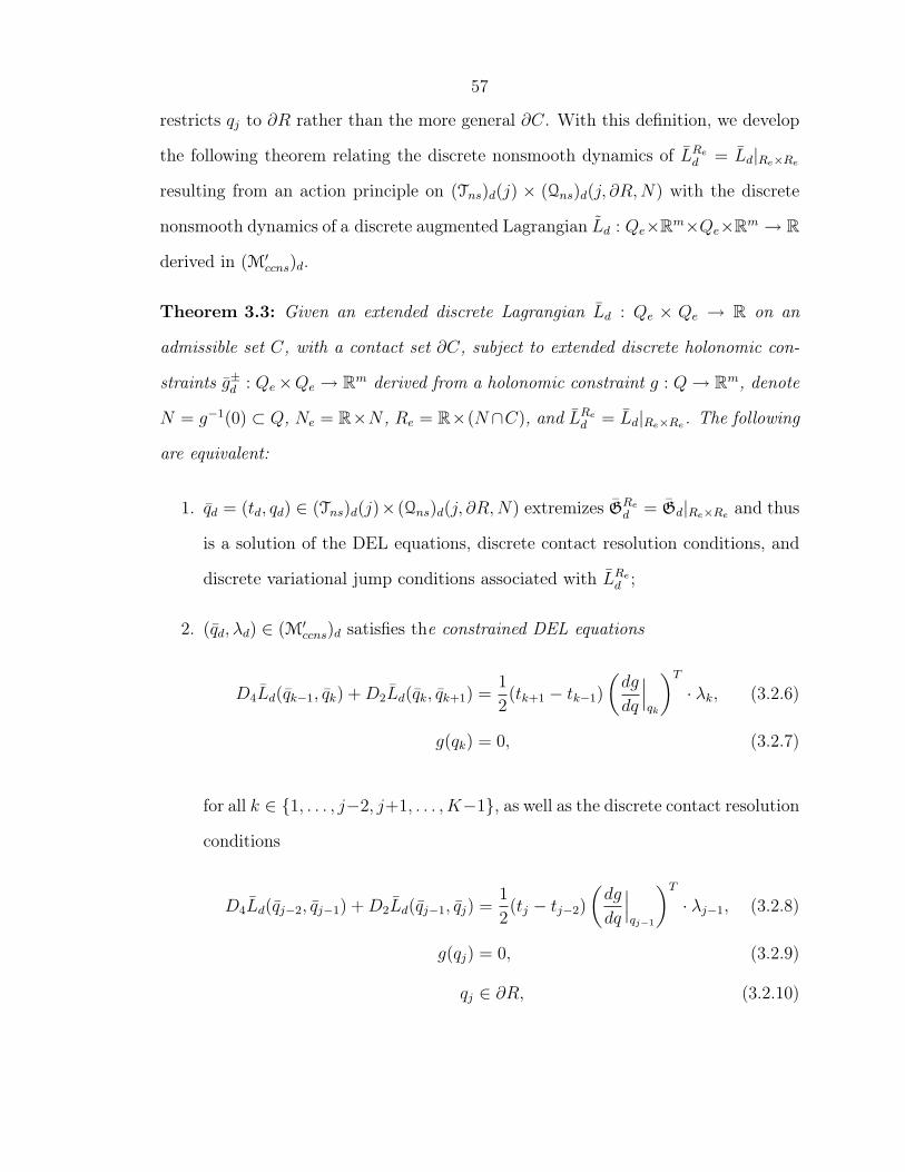
57

restricts qj to !R rather than the more general !C. With this definition, we develop

the following theorem relating the discrete nonsmooth dynamics of LRed = Ld|Re%Re

resulting from an action principle on (Tns)d(j) # (Qns)d(j, !R, N) with the discrete

nonsmooth dynamics of a discrete augmented Lagrangian Ld : Qe#Rm#Qe#Rm " R

derived in (M"ccns)d.

Theorem 3.3: Given an extended discrete Lagrangian Ld : Qe # Qe " R on an

admissible set C, with a contact set !C, subject to extended discrete holonomic con-

straints g±d : Qe#Qe " Rm derived from a holonomic constraint g : Q " Rm, denote

N = g#1(0) ' Q, Ne = R#N , Re = R#(N,C), and LRed = Ld|Re%Re. The following

are equivalent:

1. qd = (td, qd) $ (Tns)d(j)# (Qns)d(j, !R, N) extremizes GRed = Gd|Re%Re and thus

is a solution of the DEL equations, discrete contact resolution conditions, and

discrete variational jump conditions associated with LRed ;

2. (qd, %d) $ (M"ccns)d satisfies the constrained DEL equations

D4Ld(qk#1, qk) + D2Ld(qk, qk+1) =1

2(tk+1 & tk#1)

"dg

dq

&&&qk

#T

· %k, (3.2.6)

g(qk) = 0, (3.2.7)

for all k $ {1, . . . , j&2, j+1, . . . , K&1}, as well as the discrete contact resolution

conditions

D4Ld(qj#2, qj#1) + D2Ld(qj#1, qj) =1

2(tj & tj#2)

"dg

dq

&&&qj!1

#T

· %j#1, (3.2.8)

g(qj) = 0, (3.2.9)

qj $ !R, (3.2.10)

58

and the discrete variational jump conditions

i$"R

9D4Ld(qj#1, qj) + D2Ld(qj, qj+1)

:= 0, (3.2.11)

D3Ld(qj#1, qj) + D1Ld(qj, qj+1) = 0, (3.2.12)

g(qj+1) = 0, (3.2.13)

where i$"R : T $Q " T $!R is the cotangent lift of the embedding i : !R " Q;

3. (qd, %d) $ (M"ccns)d extremizes Gd(qd, %d) = Gd(qd) & (%d, "(qd))l2 and hence

solves the DEL equations for the augmented discrete Lagrangian Lgd : Qe #

Rm #Qe # Rm " R defined by

Lgd(qk, %k, qk+1, %k+1) = Ld(qk, qk+1)&

1

2(%k, g

#d (qk, qk+1))&

1

2(%k+1, g

+d (qk, qk+1)).

Proof: For the final time, we walk through an application of Theorem 2.2. Here,

the full space M is (M"ns)d and the function to be extremized is Gd. The constraint

is specified by V = Ld with the l2 inner product. Set " : M " V as "d(qd)(k) =

12(g

+d (qk#1, qk) + g#d (qk, qk+1)) = 1

2(tk+1 & tk#1)g(qk) for all k $ {1, . . . , (K & 1)} and

at the endpoints "d(qd)(0) = 12 g

#d (q0, q1) and "d(qd)(K) = 1

2 g+d (qK#1, qK). This def-

inition of " is such that qd $ (Tns)d(j) # (Qns)d(j, !R, N) if and only if "d(qd) = 0.

From this, it follows D = "#1d (0) = (Tns)d(j)# (Qns)d(j, !R, N).

The first condition above corresponds with the first condition in Theorem 2.2.

That is, qd $ D is an extremum of Gd|D. By the Lagrange multiplier theorem,

this is equivalent to (qd, %d) $ M # V being an extremum of Gd(qd, %d) = Gd(qd) &

(%d, "d(qd)). Identifying M#V with (M"ccns)d, the particular form of Gd : (M"

ccns)d "

R yields an augmented Lagrangian of the same form in Theorem 3.2.

In order to show the second and third conditions are equivalent, we evaluate

dGd = 0 using the same procedure as in Subsection 3.2.1. Using the definitions for

59

qk, ( ¨Qe)d, -ELd, and !±Lg

from Theorem 3.2, we express variations dGd · $(qd, %d) as

dGd(qd, %d) · $(qd, %d) =j#18

k=1

-ELd(qk#1, qk, qk+1) · $(qk, %k)

+K#18

k=j+1

-ELd(qk#1, qk, qk+1) · $(qk, %k)

+ !+Lg

d

(qK#1, qK) · ($qK#1, $qK)&!#Lg

d

(q0, q1) · ($q0, $q1)

+ [D4Lgd(qj#1, qj) + D1L

gd(qj, qj+1)] · $tj

+ i$(D5Lgd(qj#1, qj) + D2L

gd(qj, qj+1)) · $qj

+ [D3Lgd(qj#1, qj) + D6L

gd(qj, qj+1)] · $%j.

The expression above marks our first usage of the slot derivative notation on the

augmented discrete Lagrangian Lgd. Notice that this notation is simply shorthand

for the terms that appear in the expansion of -ELd shown in Theorem 3.2. Using the

same arguments regarding stationarity from that theorem, the expression above yields

(3.2.6), (3.2.7), (3.2.8), (3.2.9), (3.2.10), (3.2.11), (3.2.12), and (3.2.13). Equation

(3.2.11) is presented without the presence of constraint forces due to the simplification

i$"R

21

2(tj+1 & tj#1)

"dg

dq

&&&qj

#T

· %j

3= 0,

for all qj $ !R. !

In terms of integrating the discrete dynamics above, the same procedure as in

Subsection 3.2.1 applies. One integrates according to (3.2.6) and (3.2.7) until qk+1 /$ C

is found. At this point, k = j & 1 and (3.2.8), (3.2.9), (3.2.10) are solved for tj, qj,

and %j#1. Knowing the impact time and configuration, (3.2.11), (3.2.12), and (3.2.13)

are solved for qj+1 and %j. Following this, the system can be integrated according

to (3.2.6) and (3.2.7) until another impact occurs. Figure 3.2 depicts a discrete path

60

Figure 3.2: A holonomically constrained discrete path qd capturing an elastic collisionusing discrete variational jump conditions.

subject to the collision model above.

Given the null space matrix P"R(q) : Rn#m#1 " Tq!R as defined in Subsection

2.2.2, the momentum balance (3.2.11) in the discrete variational jump conditions may

be expressed equivalently as

P T"R(qj)


,= 0. (3.2.14)

Also note, as discussed in Subsection 3.1.2, the null space matrix P (q) can be applied

to the constrained DEL equations (3.2.6) for all for all k $ {1, . . . , j&2, j+1, . . . , K&

1}.

3.3 Forced and Lossful Collisions

Here, we incorporate the contact force fields of Section 2.3 into the discrete dynam-

ics. As a contact force field yields a discrete term in the continuous-time Lagrange-

d’Alembert principle, its incorporation into the discrete Lagrange-d’Alembert princi-

ple is remarkably easy.

61

3.3.1 Free Systems

In the spirit of Subsection 2.3.1, we define a discrete contact force field (F "C)d :

Qe # R# !C " T $(R# !C) to model nonconservative forces in the discrete impact

dynamics. Incorporating this force into the discrete Lagrange-d’Alembert principle

provides

dGd(qd) · $qd + (F "C)d(qj#1, qj) · $qj = 0.

The contact force only influences the stationarity conditions resulting from varia-

tions $qj, that is, the discrete variational jump conditions (3.2.3) and (3.2.4). In the

presence of (F "C)d, these are modified as

i$(D4Ld(qj#1, qj) + D2Ld(qj, qj+1) + (F "Cq )d) = 0, (3.3.1)

D3Ld(qj#1, qj) + D1Ld(qj, qj+1) + (F "Ct )d = 0, (3.3.2)

where ((F "Ct )d, (F "C

q )d) denote the corresponding components of (F "C)d. These jump

conditions maintain the structure of the continuous (2.3.1), capturing the change in

system energy and momentum tangent to !C across the impact.

As one might expect, given the null space matrix P"C(q) : Rn#1 " Tq!C, we have

P T"C(qj)

+D4Ld(qj#1, qj) + D2Ld(qj, qj+1) + (F "C

q )d

,= 0, (3.3.3)

which is equivalent to (3.3.1).


To apply a discrete contact force field to a constrained system, define (F "R)d : Qe #

R#!R " T $(R#!R). This force field modifies the jump conditions (3.2.11), (3.2.12),

62

and (3.2.13) to provide

i$"R

9D4Ld(qj#1, qj) + D2Ld(qj, qj+1) + (F "R

q )d

:= 0, (3.3.4)

D3Ld(qj#1, qj) + D1Ld(qj, qj+1) + (F "Rt )d = 0, (3.3.5)

g(qj+1) = 0. (3.3.6)

Similar to the continuous case, these results are invariant under the substitution

(F "R)d " (F "C)d.

Given the null space matrix P"R(q) : Rn#m#1 " Tq!R, we have

P T"R(qj)

+D4Ld(qj#1, qj) + D2Ld(qj, qj+1) + (F "R

q )d

,= 0, (3.3.7)

which is equivalent to (3.3.4).

3.4 Perfectly Plastic Impacts

Having established the discrete variational jump conditions for lossful impacts, we

turn our attention to deriving discrete dynamics for the perfectly plastic impacts

of Section 2.4. The task is slightly more involved than the continuous case, largely

because discrete jump conditions apply over an interval of time [(j & 1)h, jh] rather

than an instant in time. As a result, the action from pre- and post-impact constraints

may influence the jump conditions. To accurately capture this influence, we return

to the discrete Lagrange-d’Alembert principle, which will be modified in accordance

with the discrete pre- and post-impact distributions D#d and D+

d on the discrete

phase space Q#Q.

63

3.4.1 Free Systems

Given S as defined in Subsection 2.4.1, we will define jump conditions connecting

discrete dynamics on D#d = C # C and D+

d = S # S. Recalling Remark 2.9, we

will join two discrete variational principles at the impact time to provide the desired

jump conditions. In preparation for this process, consider the path space (Mns)d#L"d

where (Mns)d is as defined before and

L"d =

6%d : {0, 1, . . . , (K & 1), K} " Rp

7.

Consider a modification of (Mns)d # L"d in which we identify 0 with j and disre-

gard all elements qk if k < j. We will refer to this new path space as (Mccns)+d ,

such that for a path q+d = (q+

d , %+d ) $ (Mccns)

+d we can identify it with its image

(tj, qj, . . . , qK , %j, . . . ,%K). Similarly, consider a modification to (Mns)d in which we

identify K with j and disregard all elements qk if k > j. We will refer to this new

path space as (Mns)#d , such that for a path q#d = (t#d , q#d ) $ (Mns)

#d we can identify

it with its image (tj, q0, . . . , qj). Using these modifications, we will concern ourselves

with the combined path space (M1)±d of the form

(M1)±d = {(q#d , q+

d ) | q#d $ (Mns)#d , q+

d $ (Mccns)+d , q#d (j) = q+

d (j)}.

Elements in this path space have the property that the impact time and configuration

qj = (tj, qj) is identically represented in both paths q#d and q+d . This is essentially a

discrete notion of continuity when connecting these paths at the impact node.

Using the combined path space, define the combined discrete action ˜Gd :

(M1)±d " R of the form

˜Gd(q#d , q+

d ) =j#18

k=0

Ld(qk, qk+1) +K#18

k=j

LgSd (qk, qk+1),

64

where LgSd is the augmented discrete Lagrangian associated with the constraint gS.

This discrete action approximates the sum of the action integrals from the two vari-

ational principles we connected in the continuous case, one for unconstrained lossful

collisions and one for smooth constrained systems. All that remains is to incorporate

the contact force field to provide a discrete Lagrange-d’Alembert principle of the form

d ˜Gd(q#d , q+

d ) · $(q#d , q+d ) + (F "C)d(qj#1, qj) · $qj = 0.

It should be apparent that results away from the impact remain una!ected. That is,

the free DEL equations (3.1.3) hold for k < j& 1 and the constrained DEL equations

(3.2.6) and (3.2.7) hold on S for k > j. At k = j&1, the contact resolution equations

have the form

D4Ld(qj#2, qj#1) + D2Ld(qj#1, qj) = 0, (3.4.1)

qj $ S. (3.4.2)

Unlike the case with elastic collisions, the condition (3.4.2) is a result of stationarity.

It comes from the variations $%+j , which imply that gS(qj) = 0.

Remark 3.6: Frequently, the post-impact constraint gS is not known a priori; it is

determined by the impact configuration qj. In these cases, the contact resolution

conditions (3.2.1) and (3.2.2) may be substituted for (3.4.1) and (3.4.2) and solved

for (tj, qj), which will define gS and S. Deriving gS from qj implies that (3.4.2) will

automatically be satisfied.

65

Finally, the discrete variational jump conditions at k = j are

i$2

D4Ld(qj#1, qj) + D2Ld(qj, qj+1)

&1

2(tj+1 & tj)

"dgS

dq

&&&qj

#T

· %j + (F "Cq )d

3= 0, (3.4.3)

D3Ld(qj#1, qj) + D1Ld(qj, qj+1) + (F "Ct )d = 0, (3.4.4)

gS(qj+1) = 0. (3.4.5)

As in the continuous case, we view the condition (3.4.5) as a constraint on the allow-

able force fields (F "C)d.

The constraint term that appears in (3.4.3) may seem out of place considering that

the continuous parallel of that equation is the momentum component of (2.3.1). In

fact, this term is the reason for developing the Lagrange-d’Alembert principle above

rather than using the existing lossful collision results (3.3.1) and (3.3.2). Since the

discrete variational jump conditions result from stationarity of the action sum over

intervals of time, the work of the constraint forces associated with gS over the time

interval [tj, jh] must be accounted for.

To derive a discrete version of the impact model (2.4.3) that will satisfy the discrete

variational jump conditions above, first consider the discretization of (2.4.1). This

takes the form

D4Ld(qj#1, qj) + D2Ld(qj, qj+1)&1

2(tj+1 & tj)

"dgS

dq

&&&qj

#T

· %j + FCd = 0, (3.4.6)

where FCd : C # C " T $C has been substituted for our common notion of a discrete

contact force field. As we did in the continuous setting, consider

FCd =

"!gS

!q

#T

· %C ,

66

such that (3.4.6) reduces to

D4Ld(qj#1, qj) + D2Ld(qj, qj+1) +

"dgS

dq

&&&qj

#T

·"

%C & 1

2(tj+1 & tj)%j

#= 0.

This condition, in conjunction with gS(qj+1), provides an underdetermined system in

the variables qj+1, %j, and %C . This is representative of our inability to distinguish

any di!erence between impact forces %C and constraint forces %j in the present model.

Given a null space matrix PS(q) : Rn#p " TqS, we overcome this di"culty by using

P TS (qj)


,= 0, (3.4.7)

gS(qj+1) = 0, (3.4.8)

which is a set of n equations, presumably solvable for qj+1.

As was the case with solutions of the continuous (2.4.3), though the impact model

using (3.4.7) and (3.4.8) was not derived with a variational principle, it does constitute

a solution to the variational jump conditions (3.4.3), (3.4.4), and (3.4.5). This is

presuming we plug solutions qj+1 of (3.4.7) and (3.4.8) into (3.4.3) and (3.4.4) to

define (F "C)d.


Given U as defined in Subsection 2.4.2, we will define jump conditions connecting

discrete dynamics on D#d = R#R and D+

d = U#U . Using the same approach as in the

previous subsection, consider a modification of (M"ccns)d in which we identify K with j

and disregard all elements qk if k > j. We will refer to this new path space as (M"ccns)

#d ,

such that for a path q#d = (q#d , %#d ) $ (M"ccns)

#d we can identify it with its image

(tj, q0, . . . , qj, %0, . . . ,%j#1, %#j ). Similarly, consider a modification to (M"

ns)d # L"d in

which we identify 0 with j and disregard all elements qk if k < j. We will refer to this

67

new path space as (M"ccns)

+d , such that for a path q+

d = (q+d , %+

d ) $ (M"ccns)

+d we can

identify it with its image (tj, qj, . . . , qk, %+j , %j+1, . . . ,%K). Using these modifications,

we will concern ourselves with the combined path space (M2)±d of the form

(M2)±d = {(q#d , q+

d ) | q#d $ (M"ccns)

#d , q+

d $ (M"ccns)

+d , q#d (j) = q+

d (j)}.

Elements of this path space have Lagrange multipliers %k $ Rm for k < j and %k $ Rp

for k > j. At k = j, there exists one of each type, %#k $ Rm and %+k $ Rp.

Using the combined path space, define the combined discrete action ˜Gd :

(M2)±d " R of the form

˜Gd(q#d , q+

d ) =j#18

k=0

Lgd(qk, qk+1) +

K#18

k=j

LgUd (qk, qk+1),

where Lgd and LgU

d are the augmented discrete Lagrangians associated with g and gU ,

respectively. This discrete action approximates the sum of the action integrals from

the two variational principles we joined in the continuous case, one for constrained

lossful collisions and one for smooth constrained systems. Similar to Subsection 3.4.1,

the discrete Lagrange-d’Alembert principle takes the form

d ˜Gd(q#d , q+

d ) · $(q#d , q+d ) + (F "R)d(qj#1, qj) · $qj = 0.

This principle implies that the constrained DEL equations (3.2.6) and (3.2.7) hold on

N for k < j & 1 and again on U for k > j.

68

At k = j & 1, the contact resolution equations have the form

D4Ld(qj#2, qj#1) + D2Ld(qj#1, qj) =1

2(tj & tj#2)

"dg

dq

&&&qj!1

#T

· %j#1, (3.4.9)

g(qj) = 0, (3.4.10)

qj $ U. (3.4.11)

Note that the condition (3.4.10) is redundant as (3.4.11) implies g(qj) = 0 by the

property U . !R ' R ' N .

Lastly, the discrete variational jump conditions at k = j are

i$"R

2D4Ld(qj#1, qj) + D2Ld(qj, qj+1)&

1

2(tj & tj#1)

"dg

dq

&&&qj

#T

· %#j

&1

2(tj+1 & tj)

"dgU

dq

&&&qj

#T

· %+j + (F "R

q )d

3= 0, (3.4.12)


gU(qj+1) = 0. (3.4.14)

As in the continuous case, we view the condition (3.4.14) as a constraint on the

allowable force fields (F "R)d.

The first of the two constraint terms that appears in (3.4.12) is negligible as a

result of

i$"R

2&1

2(tj & tj#1)

"dg

dq

&&&qj

#T

· %#j

3= 0.

The second of the two constraint terms presents the same challenges as the constraint

associated with gS in (3.4.3). We treat it similarly.

69

Consider the adaptation of (3.4.6) to the constrained case with the form

D4Ld(qj#1, qj) + D2Ld(qj, qj+1)&1

2(tj & tj#1)

"dg

dq

&&&qj

#T

· %#j

& 1

2(tj+1 & tj)

"dgU

dq

&&&qj

#T

· %+j + FR

d = 0, (3.4.15)

where FRd : R # R " T $R has been substituted for our common notion of a discrete

contact force field. One way to handle the pre-impact constraint term, which follows

the methods for discrete Hamiltonian systems with constraints in [68], is to apply the

projection QN(q) : T $q Q " &N(T $

q N) to produce

QN(qj) · D4Ld(qj#1, qj) + D2Ld(qj, qj+1)&1

2(tj+1 & tj)

"dgU

dq

&&&qj

#T

· %+j + FR

d = 0.

This projection is justified with the argument that the pre-impact right discrete mo-

mentum should lie in T $N . If this is true, it holds

D4Ld(qj#1, qj)&1

2(tj & tj#1)

"dg

dq

&&&qj

#T

· %#j = QN(qj) · D4Ld(qj#1, qj),

and thus substitution into (3.4.15) is appropriate.

At this point, we follow the treatment shown in Subsection (3.4.1). That is, we

assume

FRd =

"!gU

!q

#T

· %R,

such that (3.4.15) further reduces to

QN(qj) · D4Ld(qj#1, qj) + D2Ld(qj, qj+1) +

"dgU

dq

&&&qj

#T

·"

%R & 1

2(tj+1 & tj)%

+j

#= 0.

Using the null space matrix PU(q) : Rn#p " TqU and appending the condition

70

gU(qj+1) = 0, we have the constrained version of (3.4.7) and (3.4.8) as

P TU (qj)

+QN(qj) · D4Ld(qj#1, qj) + D2Ld(qj, qj+1)

,= 0, (3.4.16)

gU(qj+1) = 0. (3.4.17)

These n equations constitute a set of sequential projections, presumably solvable for

qj+1. First, the pre-impact discrete momentum is restricted to T $N according to

the pre-impact constraint. Second, the jump condition’s entire momentum balance

is projected onto T $U as all pre-impact momentum outside of this space will be

annihilated by the impact.

The impact model (3.4.16) and (3.4.17) constitutes a solution to the variational

jump conditions (3.4.12), (3.4.13) and (3.4.14). Inserting solutions qj+1 into (3.4.3)

and (3.4.4) recovers the (F "R)d that defines this model.

3.5 Transition of Constraints

Lastly, we provide a discrete model for the transition of constraints described in

Section 2.5. As in Subsection 3.4.1, we will use S such that D+d = S # S. We

permit D+d ! R # R since the constraint g associated with R will not be enforced

following impact. As in the elastic and perfectly plastic cases for constrained systems,

D#d = R#R.

We will retain the combined path space (M2)±d as well as the combined discrete

action ˜Gd : (M2)±d " R, although now enforcing gS post-impact rather than gU . In

accordance with D#d = R#R, the constrained DEL equations (3.2.6) and (3.2.7) hold

on N for k < j & 1. At k = j & 1, the contact resolution equations have the form of

(3.4.9) and (3.4.10), but with qj $ S in place of (3.4.11).

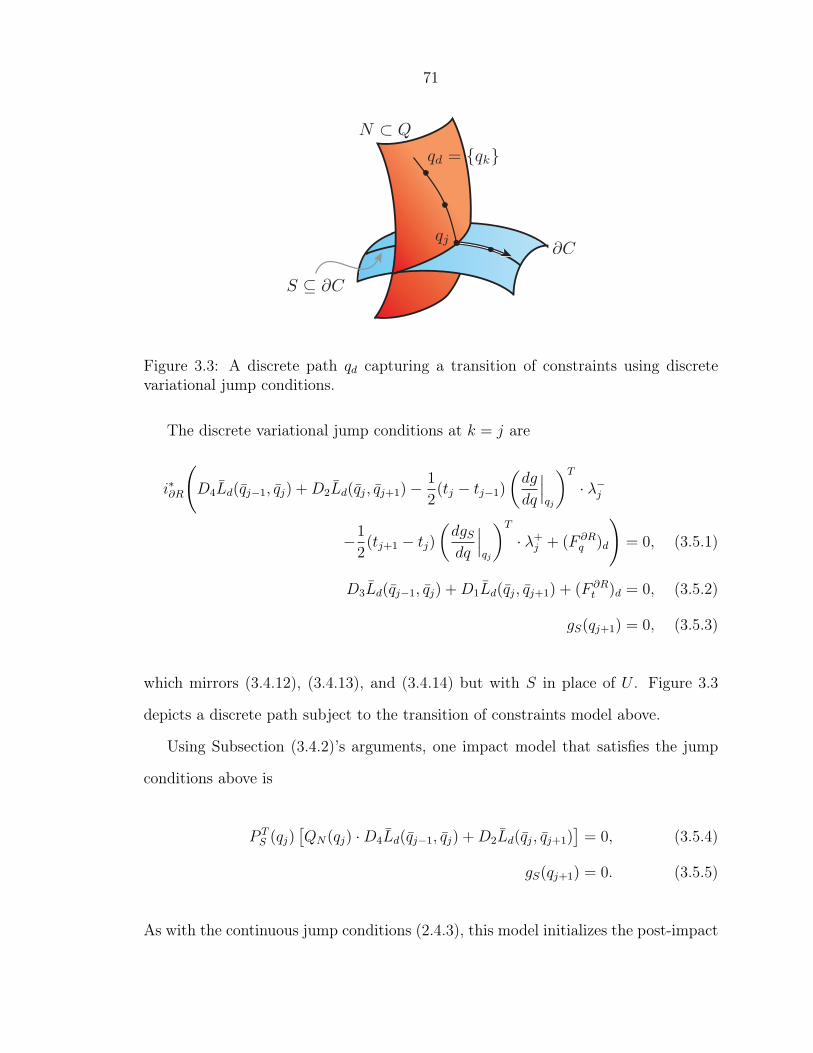
71

Figure 3.3: A discrete path qd capturing a transition of constraints using discretevariational jump conditions.

The discrete variational jump conditions at k = j are

i$"R

2D4Ld(qj#1, qj) + D2Ld(qj, qj+1)&

1

2(tj & tj#1)

"dg

dq

&&&qj

#T

· %#j

&1

2(tj+1 & tj)

"dgS

dq

&&&qj

#T

· %+j + (F "R

q )d

3= 0, (3.5.1)


gS(qj+1) = 0, (3.5.3)

which mirrors (3.4.12), (3.4.13), and (3.4.14) but with S in place of U . Figure 3.3

depicts a discrete path subject to the transition of constraints model above.

Using Subsection (3.4.2)’s arguments, one impact model that satisfies the jump

conditions above is

P TS (qj)

+QN(qj) · D4Ld(qj#1, qj) + D2Ld(qj, qj+1)

,= 0, (3.5.4)

gS(qj+1) = 0. (3.5.5)

As with the continuous jump conditions (2.4.3), this model initializes the post-impact

72

Figure 3.4: A simple rigid body wedge model.

discrete momenta at zero in all directions normal to R. Upon implementing this model

or any other that meets the condition (qj, qj+1) $ D+d = S # S, the system obeys the

constrained DEL equations (3.2.6) and (3.2.7) on S for k > j.

3.5.1 Variational Collision Integration Example

The discrete dynamics in the previous subsection provide a variational collision inte-

grator (VCI) for the transition of constraints behavior. Since this VCI will be utilized

for modeling bipedal robots in the subsequent Chapters 4 and 5, here we examine

an example of its usage. Specifically, the behavior of the rigid body wedge pictured

in Figure 3.4 undergoing a transition of constraints is captured with the VCI and

compared with a benchmark simulation.

The free configuration space Q for the wedge is 3-dimensional with coordinates

(x1, y1, "1). Note that the angle ' pictured in the model is just a relevant constant,

' = arctan(1

3/2). Physically we model the wedge in frictional contact with the line

y = 0, first with its left “foot” and then transitioning to its right “foot.” Geometrically,

73

this means that prior to impact the wedge evolves on

R =

;q

&&&& x1 &<

7

16L1 cos(" + ') = 0, y1 &

<7

16L1 sin(" + ') = 0, "1 % 0

=.

Presuming a clockwise rotation, the wedge eventually reaches the boundary !R where

"1 = 0. After undergoing the transition of constraints the system evolves on

S =

;q

&&&& x1 +

<7

16L1 cos(" & ')& L1 = 0, y1 +

<7

16L1 sin(" & ') = 0

=.

The Lagrangian for this system has the form L(q, q) = qT Mq & V (q), where M

is the diagonal 3 # 3 mass matrix defining the system’s kinetic energy and V (q) is

the gravitational potential energy. Using m to signify the total mass of the wedge

and assuming the rods that compose the wedge are isotropic and infinitely thin, the

diagonal elements of M are (m, m, J) where

J =13

48mL2

1.

The potential energy of the wedge is V (q) = mgy1, where g is the gravitational

constant. In simulation, the following parameter values were used: m = 2 kg, L1 = 0.2

m, and g = 9.81 m/s2.

For the purpose of comparison with VCI, a benchmark simulation was produced

by taking an analytical solution to the continuous time jump conditions (2.4.3) and

integrating the pre-impact phase backward in time and the post-impact phase for-

ward in time. This practice of patching intervals of smooth integration together

with analytical jump conditions is representative of the hybrid systems approach

for nonsmooth systems [41, 4]. For the smooth patches of integration, the bench-

mark simulation utilized the variational Störmer-Verlet method with a timestep of

h = (tk+1 & tk) = 4 # 10#4 s. Though the choice is not unique [68], one discrete

74

0 0.1 0.2−0.2

0.2

0.6

1

BenchmarkVCI

0 0.05 0.10.05

0.1

0.15

BenchmarkVCI

Figure 3.5: Evolution of the wedge’s center of mass in the plane (left) and orientationover time (right) for the benchmark and VCI simulations.

Lagrangian that produces Störmer-Verlet is

Ld(qk, qk+1) =tk+1 & tk

2

2L

"qk,

qk+1 & qk

tk+1 & tk

#+ L

"qk+1,

qk+1 & qk

tk+1 & tk

#3.

The VCI simulation utilized this same discrete Lagrangian, but was initialized at t = 0

rather than the contact time. The VCI simulation used a timestep of h = 1# 10#2.

Position and orientation results comparing the simulations are shown in Figure 3.5.

Initially evolving on R, the VCI detected an inadmissible configuration with "1 < 0

after the sixteenth timestep. Thus, the integrator set j = 16 and solved for qj $ !R

(with "1 = 0) and tj = 0.158 s. This evaluation of the collision time matches that used

by the benchmark within 3.75 # 10#5 s. Using the jump conditions (3.5.4), (3.5.5),

the VCI determined the first post impact configuration qj+1 $ S and then continued

integration on S where "1 < 0 is permitted. It should be noted that even with the

use of a larger timestep in the smooth regimes and adaptive timestepping through

the collision, the VCI closely matches the behavior determined by the benchmark

simulation. This matching behavior is further supported by the energy plot in Figure

3.6. The change in the discrete energy of the VCI simulation through the jump

75

0 0.05 0.1 0.15 0.2 0.251.5

2

2.5

3

3.5

4

BenchmarkVCI

Figure 3.6: Energy behavior and snapshots of the wedge progressing through a tran-sition of constraints. The VCI accurately captures the loss in kinetic energy resultingfrom collision. The slowing of the system is reflected in the snapshots, which havebeen taken from the VCI simulation at even 0.06 s intervals.

conditions, (F "Rt )d, matches the benchmark’s analytical solution within 1.41 # 10#3

percent error.

A final note is made regarding post-processing steps for the VCI simulation. Since

holonomic constraints have been used to model frictional contacts, it must be checked

that all contacts have been accounted for and only feasible contacts have been sim-

ulated. For the model above, the wedge is a single rigid body and there is only one

contact surface in the plane. Hence, there is only one type of contact, rigid body

to surface, which has been accounted for in all instances. In terms of feasibility, it

must be checked that the unconstrained acceleration of any points of contact are per-

sistently “into” the contact surface, the frictional constraint forces tangential to the

contact surface fall within some physically realizable bounds, and at no point has the

paradox of Painlevé [85] been encountered. For the simple wedge, no red flags were

raised in post-processing. Note that if a simulation fails one of these post-processing

checks it does not stonewall the VCI method. It simply implies an additional behav-

ior, a collision or perhaps a constraint release, must be added to the model.

76

Chapter 4

Discrete Nonsmooth Mechanics andOptimal Control

In this chapter, we extend the structured integration results of Chapter 3 to generate

optimal controls for nonsmooth mechanical systems. Optimal control generation is

done according to the method of discrete mechanics and optimal control (DMOC) [47,

48, 51, 62, 52], which relies on variational integrators to discretize standard optimal

control problems. After a review of DMOC for smooth systems, we describe the

modifications necessary to incorporate nonsmooth impact mechanics. The nonsmooth

version of DMOC is demonstrated in the task of determining locally optimal gaits for

bipedal robot models.

4.1 The DMOC Method

First introduced in [47], the DMOC method uses discrete mechanics to recast stan-

dard optimal control problems in discrete time. The discretized problem has the

structure of an equality-constrained nonlinear optimization problem and is solvable

with sequential quadratic programming (SQP) methods [36].

77

4.1.1 Smooth Systems

In the traditional case for DMOC we assume we are dealing with smooth mechanical

systems as in Section 2.1, and thus inherit the definitions of Q, TQ, and L from that

section. The continuous time optimal control problem solved by DMOC seeks the

local minima of a cost function J while using controls u : R " T $Q to move the

mechanical system from a given initial phase (q0, q0) to a given final phase (qT , qT )

in a specified time T . It is assumed that J is the integral of a performance metric

Z : $ " R where

$ =6((q1, v1), (q2, u2)) $ TQ# T $Q | q1 = q2

7.

For brevity we write elements of $ excluding the redundant coordinate in Q. Using

this notation the optimal control problem is formally stated

Minimize J(q(t), u(t)) =

! T

0

Z(q(t), q(t), u(t)) dt,

subject to (q(0), q(0)) = (q0, q0), (q(T ), q(T )) = (qT , qT ), and the appropriate forced

Euler-Lagrange equations of motion. Treating u as an external force field Fq, the

system dynamics have precisely the form of (2.1.16).

Using the machinery from 3.1, the DMOC method moves all aspects of the problem

above to the discrete time setting. That is, q(t) is replaced by a discrete path qd $

Qd(Q) and the influence of u(t) is captured with ud = {u±k }, a discrete path of left

and right discrete forces u±k : Q#Q " T $Q at each time node. Similar to the discrete

forces F±d defined in Subsection 3.1.3, the u±k provide the approximation

u#k · $qk + u+k · $qk+1 0

! tk+1

tk

u(t) · $q(t) dt.

The boundary conditions (q0, q0) and (qT , qT ) are discretized through a combina-

78

tion of continuous and discrete Legendre transformations. Following the treatment

in [47], we make use of the standard Legendre transformation FL : TQ " T $Q

defined as

FL(q, q) = (q, D2L(q, q)),

as well as the left and right discrete Legendre transforms Fu±Ld : Q#Q " T $Q

defined as

Fu+Ld(qk, qk+1) = (qk+1, D2Ld(qk, qk+1) + u+k ),

Fu#Ld(qk, qk+1) = (qk,&D1Ld(qk, qk+1)& u#k ).

With these definitions, we enforce the boundary conditions at the momentum level

(in T $Q) as

(q0, D2L(q0, q0)) = (q0,&D1Ld(q0, q1)& u#0 ), (4.1.1)

(qT , D2L(qT , qT )) = (qK , D2Ld(qK#1, qK) + u+K#1). (4.1.2)

For a discrete time approximation of J , we follow the same method by which we

approximated the action map G with Gd in Subsection 3.1.1. That is, we introduce

a discrete performance metric Zd : T $Q# T $Q " R providing the approximation

Zd(qk, u#k , qk+1, u

+k ) 0

! tk+1

tk

Z(q(t), q(t), u(t)) dt.

Using Zd we approximate J with a discrete cost function Jd and state the discretized

optimal control problem:

Minimize Jd(qd, ud) =N#18

k=0

Zd(qk, u#k , qk+1, u

+k ),

79

subject to (4.1.1), (4.1.2), and the appropriate forced DEL equations of motion. Treat-

ing u±k as a discrete external force field (Fq)±d , the system dynamics have precisely the

form of (3.1.10). As mentioned, this discretized problem is an equality-constrained

nonlinear optimization problem and can be solved using SQP.

4.1.2 Nonsmooth Systems

In this subsection, we extend the DMOC method to handle systems with collisions.

To simplify the process, we assume advanced knowledge of the number of collisions

Nc to take place in the time interval [0, T ], the set of collision times {t$} where

( $ {1, . . . , Nc}, and the desired collision model (elastic, lossful, perfectly plastic) to

be enforced at each t$.

Remark 4.1: Generalizing the following method to problems with a variable number

of collisions, variable collision times, or variable collision models could be achieved

with the use of dynamic programming, but remains outside the scope of this thesis.

The search for optimal trajectories will only be performed in the space of admis-

sible configurations, giving rise to the constraint q(t) $ C for all t $ [0, T ]. Further-

more, we require that at the collision times t$, the corresponding system configura-

tion is on the contact set !C. We express this constraint as g"C(q(t$)) = 0 for all

( $ {1, . . . , Nc}.

Using the assumptions and constraint definitions above, we modify the continuous

time optimal control problem as

Minimize J(q(t), u(t)) =

! T

0

Z(q(t), q(t), u(t)) dt,

subject to (q(0), q(0)) = (q0, q0), (q(T ), q(T )) = (qT , qT ), the appropriate forced Euler-

Lagrange equations of motion, q(t) $ C for all t $ [0, T ], g"C(q(t$)) = 0 for all

( $ {1, . . . , Nc}, and the appropriate variational jump conditions at each t$.

80

All of the elements of this optimization problem held in common with the problem

for smooth systems are discretized in the same fashion as in the previous subsection.

To handle the collisions, we require that the mesh of time has been defined such that

each t$ has an associated time node tk. In this case, we discretize the admissibility

constraint q(t) $ C as g"C(qk) " 0 for all k $ {0, . . . , K} and the contact conditions

q(t$) $ !C as g"C(qk) = 0 for all k $ {k | tk = t$, ( $ {1, . . . Nc}}. Additionally,

we enforce the discrete variational jump conditions associated with the appropriate

collision model at each tk associated with some t$. These discrete variational jump

conditions replace the forced DEL equations at these nodes.

As a final note, we mention that in practice the added constraints for the nons-

mooth case, both equality and inequality, do not change the solution method. The

nonsmooth version of DMOC is still solvable with SQP.

Remark 4.2: Though it is not regularly stated, admissibility constraints similar to

g"C(qk) " 0 are frequently used in DMOC for smooth systems to prevent mass inter-

section and other physical impossibilities.

Remark 4.3: The variational jump conditions presented in Chapter 3 were absent

of external forcing. To accurately capture the influence of the control forces u through

collisions, one simply extends the theory of Subsection 3.1.3 to the nonsmooth cases

in Sections 3.2, 3.3, 3.4, and 3.5.

4.2 Optimal Gait Search for Bipedal Robots

In this section, we describe a specific usage of the DMOC method for nonsmooth

systems in regards to bipedal robot models. Results are presented for two 4-link rigid

body biped models, a six-degree-of-freedom planar model and an eleven-degree-of-

freedom model in three dimensions.

81

4.2.1 Bipedal Gait Optimization Problem

In this specific application of the DMOC method, we seek locally optimal periodic

gaits for a given biped model. The cost function we will locally minimize is the

specific cost of transport [30], a standard metric in locomotion problems defined

as

& =

! T

0

Pcontrol

Wrobot · Vfwddt,

where Pcontrol is the instantaneous power exerted by the control forces, Wrobot is the

total weight of the robot, and Vfwd is the forward velocity of the center of mass. In

our analysis to come, we will assume T is the period of a single step. This means we

can recast the integral form above as

& =Econtrol

Wrobot · Lstep,

where Econtrol is the energy exerted by the control forces over the course of a step and

Lstep is the length of the step. Note that the cost & is dimensionless (the numerator

units are J, and the denominator is in N # m). It should be apparent that the

dependence of & on q(t), q(t), and u(t) follows the structure specified in the definition

of J , and thus setting J = & is permitted.

In order to search for periodic gaits, the notion of specified boundary conditions

(q0, q0) and (qT , qT ) is replaced with a periodicity relation ) : TQ " TQ such that

(q(T ), q(T )) = )(q(0), q(0)). Noting that the stance leg of a bipedal robot switches

over the course of one step, defining ) usually entails rearranging information in

the generalized coordinate system. For instance, the initial position and velocity of

the knee joint on a robot’s “right” leg will depend on the final position and velocity

of the knee joint on the robot’s “left” leg. The configuration component of ) can

be used to define a discrete periodicity relation )d : Q # Q " Q # Q such that

82

(qK#1, qK) = )d(q0, q1).

We will assume the trajectory defining the periodic gait has a single collision

(Nc = 1), which we will model using the transition of constraints jump conditions

defined in Section 2.5. Given that trajectories are periodic and contain only a single

collision per period, the choice of the collision time t$ is somewhat arbitrary. In

particular, the solution (qd, ud) for a given choice of t$ can be shifted in time to

provide a solution for other choices t$ + ah $ [0, T ], where a $ Z. Furthermore,

changing t$ by an increment other than ah may slightly change results, but not the

underlying continuous trajectory they represent.

4.2.2 4-Link Planar Biped Results

This subsection provides results from an optimal gait search for the planar biped

model shown in Figure 4.1. The free configuration space Q for this model is six-

dimensional with coordinates (x1, y1, "1, "2, "3, "4). Physically, this model has point

feet and walks along the flat line y = 0 in the plane. In the geometric terms of Section

2.5, this means that prior to impact the system evolves on

R = {q |x1 = 0, y1 = 0, y1 + L1(c1 & c123) + L2(c12 & c1234) % 0},

where we have introduced the shorthand c1 = cos("1), c12 = cos("1 + "2), c123 =

cos("1 + "2 + "3), and c1234 = cos("1 + "2 + "3 + "4). The manifold R is the set of

configurations where the position of one point foot is fixed on the contact surface

y = 0 and the height of the other point foot is positive (above the contact surface).

At the double-support phase, in which both point feet are on the contact surface, we

have q $ !R where

!R = {q |x1 = 0, y1 = 0, y1 + L1(c1 & c123) + L2(c12 & c1234) = 0}.

83

Figure 4.1: A 4-link planar biped model.

Following impact, the biped has established a new stance foot and evolves on

S = {q |x1 + L1(s123 & s1) + L2(s1234 & s12)& Lstep = 0,

y1 + L1(c1 & c123) + L2(c12 & c1234) = 0},

where we have abbreviated sine in the same fashion as cosine above.

The constant Lstep in the definition of S indicates the step length of the robot

during the double-support phase. While the DMOC framework permits changes in

this variable, for simplicity during the optimization it has been fixed at 0.56 m. The

remaining parameters in the model have been fixed in the optimization as L1 = L2 =

0.5 m, m1 = m4 = 2 kg, m2 = m3 = 3 kg, J1 = J4 = 124m1L2

1, J2 = J3 = 124m2L2

2.

Note that the moments of inertia, as defined, indicate an assumption of anisotropism

for the links (they have higher mass density towards their center). Finally, the period

of the step is fixed at T = 0.9 s and is represented in discrete time with K = 80

timesteps.

The Lagrangian for this system has a similar form as that of the example in

84

Subsection 3.5.1. That is, L(q, q) = qT M(q)q & V (q) where qT M(q)q is the kinetic

energy of the system and V (q) is the gravitational potential energy. In this case,

closed form expressions for M(q) and V (q) have a significant level of complexity.

For this reason, for the implementation of DMOC, calculations of L and its partial

derivatives were performed using the tree structure framework of [46]. Using this

method, one does not need an unwieldy analytical expression for L, as it can be

constructed from simpler rigid body Lagrangians. To move the Lagrangian L to the

discrete time setting, Ld was defined according to the midpoint rule as in (3.1.1).

During the walking motion, control torques are applied at the stance leg’s point

of contact, both knee joints, and the hip joint. Under these control inputs, the robot

is fully actuated on the respective constraint submanifolds R and S. It should be

noted, however, that an underactuated version of this problem was solved with the

DMOC method in [73].

Results from the gait search optimization are shown in Figure 4.2. The overall

small deviations in system energy (note the y axis scale on the figure) indicate an

e"cient use of work done by the control inputs. This notion is also supported by

optimal cost associated with the gait pictured, a specific cost of transport & = 1.59#

10#3. For reference, this is roughly two orders of magnitude smaller than that of

average human walking. As we will see, though, such dominance in performance may

be di"cult to maintain as additional complexity is added to the model.

As in Subsection 3.5.1, post processing steps were performed to ensure that the

model remained in the space of feasible contact forces as well as admissible configu-

rations throughout the gait. Given the weight of the robot and the permission of link

“intersections” in the plane (links may pass through one another), these conditions

represent relatively weak constraints on the gait for this model.

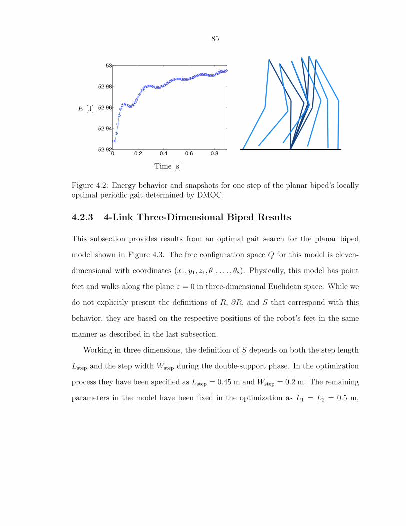
85

0 0.2 0.4 0.6 0.852.92

52.94

52.96

52.98

53

Figure 4.2: Energy behavior and snapshots for one step of the planar biped’s locallyoptimal periodic gait determined by DMOC.

4.2.3 4-Link Three-Dimensional Biped Results

This subsection provides results from an optimal gait search for the planar biped

model shown in Figure 4.3. The free configuration space Q for this model is eleven-

dimensional with coordinates (x1, y1, z1, "1, . . . , "8). Physically, this model has point

feet and walks along the plane z = 0 in three-dimensional Euclidean space. While we

do not explicitly present the definitions of R, !R, and S that correspond with this

behavior, they are based on the respective positions of the robot’s feet in the same

manner as described in the last subsection.

Working in three dimensions, the definition of S depends on both the step length

Lstep and the step width Wstep during the double-support phase. In the optimization

process they have been specified as Lstep = 0.45 m and Wstep = 0.2 m. The remaining

parameters in the model have been fixed in the optimization as L1 = L2 = 0.5 m,

86

Figure 4.3: A 4-link three-dimensional biped model with revolute joint knees and aspherical joint hip. The triple ("1, "2, "3) represents the ZYZ Euler angles of the bodyframe of first link with respect to the inertial frame, and ("5, "6, "7) represents theZYZ Euler angles of the body frame of the third link with respect to the body frameof the second.

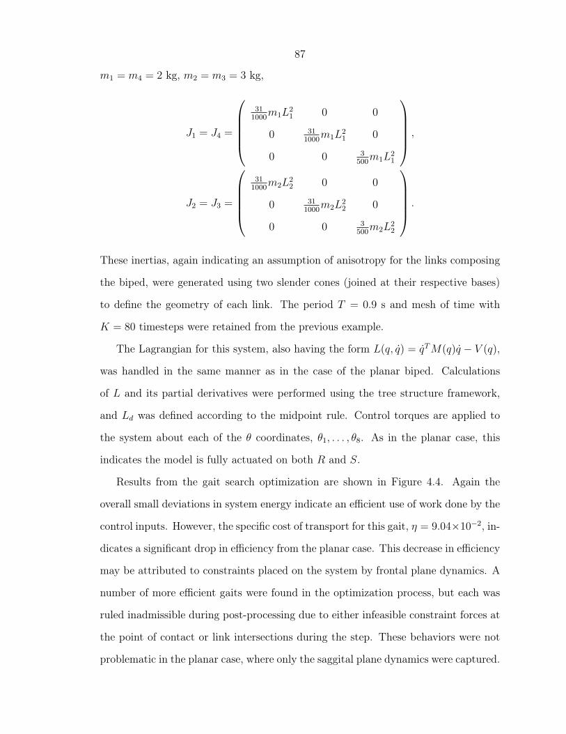
87

m1 = m4 = 2 kg, m2 = m3 = 3 kg,

J1 = J4 =

0

>>>>1

311000m1L2

1 0 0

0 311000m1L2

1 0

0 0 3500m1L2

1

4

????5,

J2 = J3 =

0

>>>>1

311000m2L2

2 0 0

0 311000m2L2

2 0

0 0 3500m2L2

2

4

????5.

These inertias, again indicating an assumption of anisotropy for the links composing

the biped, were generated using two slender cones (joined at their respective bases)

to define the geometry of each link. The period T = 0.9 s and mesh of time with

K = 80 timesteps were retained from the previous example.

The Lagrangian for this system, also having the form L(q, q) = qT M(q)q & V (q),

was handled in the same manner as in the case of the planar biped. Calculations

of L and its partial derivatives were performed using the tree structure framework,

and Ld was defined according to the midpoint rule. Control torques are applied to

the system about each of the " coordinates, "1, . . . , "8. As in the planar case, this

indicates the model is fully actuated on both R and S.

Results from the gait search optimization are shown in Figure 4.4. Again the

overall small deviations in system energy indicate an e"cient use of work done by the

control inputs. However, the specific cost of transport for this gait, & = 9.04#10#2, in-

dicates a significant drop in e"ciency from the planar case. This decrease in e"ciency

may be attributed to constraints placed on the system by frontal plane dynamics. A

number of more e"cient gaits were found in the optimization process, but each was

ruled inadmissible during post-processing due to either infeasible constraint forces at

the point of contact or link intersections during the step. These behaviors were not

problematic in the planar case, where only the saggital plane dynamics were captured.

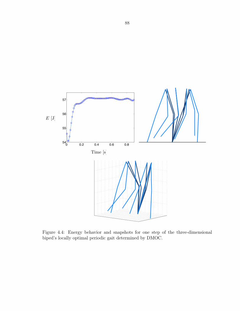
88

0 0.2 0.4 0.6 0.854

55

56

57

Figure 4.4: Energy behavior and snapshots for one step of the three-dimensionalbiped’s locally optimal periodic gait determined by DMOC.

89

It is possible that by performing further optimizations or making modifications to

the model, a more e"cient feasible gait could be identified. Additionally, the method

suggested in Remark 4.1 could rule out infeasible results during an optimization,

rather than in post-processing. In any case, the gait presented here is feasible and

more than twice as e"cient as human walking.

90

Chapter 5

Design of Dynamics Optimization

In this chapter, we present a multilayered design optimization scheme, termed design

of dynamics (DD), to determine mechanical system designs that reduce the cost of

optimal control. The scheme leverages the results of Chapter 4 by making use of

DMOC in the “inner” layer optimization. The “outer” layer, for which function eval-

uations are assumed to be costly, uses optimization with surrogate functions [45, 6].

DD results are presented for the task of optimizing the knee joint placement of the

4-link planar biped model from Subsection 4.2.2.

5.1 Design of Dynamics

Typically the task of a controls engineer is to achieve some desired performance from

a dynamical system through the use of sensors and inputs. Classically, the system

model, or plant, defining the system dynamics and available sensors/actuators is

assumed to be fixed. Modern control theory provides an impressive set of tools to

analyze and control fixed plants, and we postulate that the same tools can provide

additional benefits when utilized in the system design process. An example of this is

the following DD optimization scheme, which uses DMOC, an optimal control scheme

for fixed plants, to perform design optimization.

Formally, the problem considered by DD is that of optimizing a given set of design

91

Figure 5.1: The multilayered DD optimization scheme.

parameters * to reduce the cost of optimal control J for a given mechanical system.

We propose solving this problem using a multilayered optimization as pictured in

Figure 5.1. The “outer” loop of this scheme performs the optimization of * in design

space by making function calls to the “inner” loop. The inner loop calculates the cost

of optimal control J associated with a particular design by solving the DMOC opti-

mization problem from Section 4.1. Given that each outer loop function evaluation

requires the solution of an optimization problem, the outer loop optimization should

be performed with a method sensitive to this computational expense. The use of

surrogate functions, as described in the next section, is such a method.

Remark 5.1: In its current definition, the DD scheme is applicable to any mechan-

ical system with quantifiable design parameters that can be treated with the DMOC

method. As the class of problems handled with DMOC grows, so will the applicability

of DD.

One issue of note with the proposed DD scheme is the sensitivity of the inner loop

to the initial guess provided to SQP as it solves the DMOC problem. For DMOC

problems with many local minima, meaning many locally optimal control policies,

the cost J determined with SQP will be dependent on both the design parameters

* in use and the initial guess for qd and ud. This makes the DD scheme, as it is

currently expressed, most suitable for problems with a low number of local minima,

or at least minima with large basins of attraction relative to initial conditions. In

92

practice, there is no standard way to determine these attributes a priori for a given

DMOC problem. Thus, it remains a subject of future work to adapt the DD scheme

to handle problems with a dense population of local minima in design space, as well

as to adapt the DMOC framework to be less sensitive to the user’s initial guess.

5.2 Optimization with Surrogate Functions

In this section, we discuss the properties of surrogate function optimization methods

as motivation for their use in the outer loop of DD. In the outer loop optimization

problem, consider that there is no analytical expression for the gradient of J with

respect to *. Furthermore, the computational expense associated with outer loop

function calls implies that numerical approximations of the gradient would be imprac-

tical. It is due to these factors that standard gradient-based optimization methods,

SQP or otherwise, are not applicable in this setting. However, surrogate methods

[15, 6] have been developed to handle precisely these challenges in optimization.

The basic algorithm underlying the use of surrogate functions in optimization is

as follows. Given some function f(x) to be optimized, perform the following:

1. Choose a surrogate s that approximates f using a finite number of function

evaluations f(xi), where the samples xi belong to a finite set {x1, . . . , xd}. The

definition of s is provided by a user’s choice of interpolation or smoothing func-

tion.

2. Using some prescribed rules, determine additional sample locations. One obvi-

ous rule [6] is to calculate the minimum of s and sample there. More sophisti-

cated implementations may add randomly generated points to globally sample

the space [65].

3. Add the newly determined sample points to the set {x1, . . . , xd} and perform

93

all necessary new function evaluations f(xi).

4. Check for convergence. A criteria for convergence is typically expressed in terms

of the improvement in min f(xi) provided by the function evaluations performed

in step 3.

5. Return to step 1 and update the surrogate s. Repeat steps until convergence.

This basic algorithm provides many user freedoms, which has led to several studies

regarding customized use and expansion of the method. A means to appropriately

select an initial set of samples {x1, . . . , xd} has been examined in [77, 53]. Various

choices for basis functions defining the structure of s are compared in [45]. Conver-

gence properties, particularly those gained by incorporating pattern search methods

into the algorithm above, are examined in [15]. Also, there exists an open source

Matlab optimization package [63] that makes use of statistical kriging functions [86],

a popular choice of basis for the surrogate s.

5.3 Knee Joint Placement Optimization Results

In this section, we present results from the implementation of DD regarding the knee

joint placement of the planar bipedal robot model in Subsection 4.2.2. Here, the inner

loop optimization of DD is performed with the DMOC code from that example. The

outer loop optimization of DD is performed using the “strawman” algorithm (SA) of

[65].

SA is one of the simplest implementations of optimization with surrogate func-

tions. It is used here for illustrative purposes in spite of the performance benefits

associated with more complex surrogate methods. In terms of the steps outlined in

the previous subsection, SA restricts the sampling in step 2 to a single sample at the

minimum of the surrogate s. The remainder of the steps remain unchanged, implying

94

that SA still provides user freedoms in terms of the choice of initial samples, the

structure of the surrogate, and the criteria for convergence.

For the use of SA in the DD example to come, the one-dimensional design op-

timization was simply initialized with two samples in a promising region of design

space. The surrogate s was chosen to be a cubic spline passing through the func-

tion evaluations J(*i). Convergence was determined when the addition of a sample

produced less than a 1# 10#5 percent change in min J(*i).

To apply DD optimization in the task of knee joint placement, the biped model in

Figure 4.1 was parameterized using * = L1. The total height of the biped was kept

fixed in the design process by defining L2 = 1& * such that the biped remained 1 m

tall for all values of *. The practice of equating the cost of optimal control J and the

dimensionless specific cost of transport & was retained from Subsection 4.2.2. Results

for the DD optimization of J over * are shown in Figure 5.2.

Using SA in the outer loop, DD produced a locally optimal design in nine function

evaluations. The specific cost of transport associated with this design is & = 4.44 #

10#4, an 11.1 percent improvement over the worst of our samples J(*i) and a 72.1

percent improvement over the results in Subsections 4.2.2. Though the example

problem considered here is low dimensional, the e"ciency of DD in this instance

motivates its development for and use on problems of higher complexity.

DMOC results, in terms of energy behavior and gait snapshots, for the locally

optimal design produced by DD are pictured in Figure 5.3. As in Figure 4.2, the scale

on the energy plot indicates low overall fluctuation in system energy and e"cient use

of work done by the controls. In terms of the influence of the knee joint placement

on e"ciency, the robot seems to leverage high knees and short thighs by lowering its

stance thigh in the first half of the step. This lowering motion may make it easier to

lift the swing leg and save energy required from the controls.

95

0.8 0.85

4.4

4.6

4.8

5

x 10−4

0.8 0.85

4.4

4.6

4.8

5

x 10−4

0.8 0.85

4.4

4.6

4.8

5

x 10−4

0.8 0.85

4.4

4.6

4.8

5

x 10−4

0.8 0.85

4.4

4.6

4.8

5

x 10−4

0.8 0.85

4.4

4.6

4.8

5

x 10−4

0.8 0.85

4.4

4.6

4.8

5

x 10−4

0.8 0.85

4.4

4.6

4.8

5

x 10−4

Figure 5.2: Progression of the “strawman” surrogate method in the outer loop of DD.The optimal knee joint placement is determined in nine function evaluations.

0 0.2 0.4 0.6 0.870.42

70.425

70.43

70.435

Figure 5.3: Energy behavior and snapshots for one step of the locally optimal gait ofthe locally optimal design produced by DD.

96

Chapter 6

Future Directions

There are several future directions to pursue in order to extend the applicability and

utility of the theory and methods presented in this thesis. Though a variety of be-

haviors have been captured with variational nonsmooth mechanics here, a number of

relevant behaviors have yet to be modeled. Adding complexity to the system con-

straints (making them nonholonomic for instance) and contact conditions (examining

compliant patch contacts for instance) provides challenging important problems.

Another task is to develop more computationally feasible variational collision in-

tegration methods. The adaptive time stepping used in the integrators derived in this

thesis makes them ill suited for large systems with a high density of collision events

over time. Defining a symplectic method that captures impact mechanics using fixed

time steps would increase applicability and attract more users.

Improvements in the DMOC method for nonsmooth systems could be made in

more than one regard. As mentioned in Remark 4.1, dynamic programming could

improve the DMOC optimization process by allowing changes in collision time and

collision model within the optimization. This improvement will allow DMOC to

handle problems where the timing of impacts and behavior of the system during

impact is not known a priori.

A second improvement for DMOC is applicable to the method as a whole, not

just the nonsmooth case. Casting the DMOC problem with such a large number

97

of equality constraints (a set of DEL equations at each time node) increases com-

putational expense and can actually create additional local minima in the trajectory

optimization process. By leveraging ideas like di!erential flatness, one may be able to

decrease the dimension of the DMOC problem in terms of both optimization variables

and number of constraints.

For the DD method, improvements could be made in terms of sensitivity to inner

loop initialization. The inner loop requires both design parameters and an initial

condition to compute a cost. The outer loop is only interested in the influence of

the parameters on cost, and thus a means to minimize or remove the influence of the

inner loop initial condition must be explored.

98

Bibliography

[1] R. Abraham, J. E. Marsden, and T. S. Ratiu. Manifolds, Tensor Analysis and

Applications, volume 75 of Appl. Math. Sci. Springer-Verlag, New York, second

edition, 1988.

[2] V. Acary and B. Brogliato. Numerical Methods for Nonsmooth Dynamical Sys-

tems: Applications in Mechanics and Electronics, volume 35. Springer Lecture

Notes in Applied and Computational Mechanics, 2008.

[3] N. M. Alexandrov, J. E. Dennis, R. M. Lewis, and V. Torczon. A trust-region

framework for managing the use of approximation models in optimization. Struc-

tural Optimization, 15(1):16–23, 1998.

[4] A. D. Ames and R. D. Gregg. Stably extending two-dimensional walking to three

dimensions. In Proc. ACC, New York, 2007.

[5] C. Audet and J. E. Dennis. Analysis of generalized pattern searches. SIAM J.

on Optimization, 13(3):889–903, 2003.

[6] J. F. M. Barthelemy and R. T. Haftka. Approximation concepts for opti-

mum structural design—a review. Structural and Multidisciplinary Optimization,

5(3):129–144, 1993.

[7] H. Baruh. Analytical Dynamics. WCB/McGraw-Hill, 1999.

[8] A. Bemporad and M. Morari. Control of systems integrating logic, dynamics,

and constraints. Automatica, 35(3):407–427, 1999.

99

[9] M. Benzi, G. Golub, and J. Liesen. Numerical solution of saddle point problems.

Acta Numerica, 2005.

[10] P. Betsch and S. Leyendecker. The discrete null space method for the energy con-

sistent integration of constrained mechanical systems. II. Mulitbody dynamics.

Int. J. Num. Meth. Eng., 67:499–552, 2006.

[11] P. Betsch and P. Steinmann. Constrained dynamics of geometrically exact beams.

Comput. Mech., 31(1–2):49–59, 2003.

[12] J. T. Betts. Survey of numerical methods for trajectory optimization. AIAA J.

Guidance, Control, and Dynamics, 21(2):193–207, 1998.

[13] T. Binder, L. Blank, H. G. Bock, R. Bulirsch, W. Dahmen, M. Diehl, T. Kro-

nseder, W. Marquardt, J. P. Schlöder, and O. v. Stryk. Introduction to model

based optimization of chemical processes on moving horizons. In M. Grötschel,

S. O. Krumke, and J. Rambau, editors, Online Optimization of Large Scale Sys-

tems: State of the Art, pages 295–340. Springer, 2001.

[14] A.m. Bloch, J. Ballieul, P. Crouch, and J. E. Marsden. Nonholonomic Mechanics

and Control, volume 24. Interdisciplinary Applied Mathematics, Springer-Verlag,

2003.

[15] A. J. Booker, J. E. Dennis Jr., P. D. Frank, D. B. Serafini, V. Torczon, and

M. W. Trosset. A rigorous framework for optimization of expensive functions by

surrogates. Structural and Multidisciplinary Optimization, 17(1):1–13, 1999.

[16] N. M. Bou-Rabee and J. E. Marsden. Reduced Hamilton-Pontryagin variational

integrators. Found. Comput. Math., 9:1–23, 2008.

100

[17] M. S. Branicky, V. S. Borkar, and S. K. Mitter. A unified framework for hybrid

control: Model and optimal control theory. IEEE Trans. Auto. Control, 43(1):31–

45, 1998.

[18] K. E. Brenan, S. L. Campbell, and L. R. Petzold. Numerical Solution of Initial-

Value Problems in Di!erential-Algebraic Equations. Prentice Hall, 1989.

[19] B. Brogliato. Nonsmooth Impact Mechanics: Models, Dynamics and Control,

volume 220 of Lecture Notes in Control and Inform. Sci. Springer, New York,

1996.

[20] B. Brogliato. Nonsmooth Mechanics. Springer, 1999.

[21] B. Brogliato. On the control of non-smooth complementarity dynamical systems.

Phil. Trans. R. Soc. Lond A, 359:2369–2383, 2001.

[22] F. Bullo and M. Zefran. Modeling and controllability for a class of hybrid mechan-

ical systems. IEEE Transactions on Robotics and Automation, 18(4):563–573,

2002.

[23] G. Buttazzo and D. Percivale. On the approximation of the elastic bounce prob-

lem on riemannian manifolds. Journal of Di!erential Equations, 47:227–275,

1983.

[24] A. Chatterjee and A. Ruina. A new algebraic rigid-body collision law based on

impulse space considerations. Journal of Applied Mechanics-Transactions of the

ASME, 65(4):939–951, 1998.

[25] C. Chevallereau and Y. Aoustin. Optimal reference trajectories for walking and

running of a biped robot. Robotica, 19(5):557–569, 2001.

101

[26] C. Chevallereau, J.W. Grizzle, and C. Shih. Asymptotically stable walking for a

five-link underactuated 3D bipedal robot. IEEE Trans on Robotics, 25(1):37–50,

2008.

[27] F. Cirak and M. West. Decomposition contact response (dcr) for explicit finite

element dynamics. Int. J. for Num. Methods in Eng., 64:1078–1110, 2008.

[28] S. Collins, A. Ruina, R. Tedrake, and M. Wisse. E"cient bipedal robots based

on passive-dynamic walkers. Science, 307(5712):1082–1085, 2005.

[29] P. A. M. Dirac. On generalized hamiltonian dynamics. Can. J. Math., 2:129–148,

1950.

[30] V. Duindam. Port-Based Modeling and Control for E"cient Bipedal Walking

Robots. PhD thesis, University of Twente, 2006.

[31] R. Fetecau. Variational Methods for Nonsmooth Mechanics. PhD thesis, Cali-

fornia Institute of Technology, 2003.

[32] R. Fetecau, J. E. Marsden, M. Ortiz, and M. West. Nonsmooth lagrangian

mechanics and variational collision integrators. SIAM Journal on Dynamical

Systems, 2:381–416, 2003.

[33] A. F. Filippov. Di!erential equations with discontinuous right-hand side. Amer-

ican Mathematical Society Translations, 42:199–231, 1964.

[34] A. F. Filippov. Classical solutions of di!erential equations with multivalued

right-hand side. SIAM J. Control Optim., 5:609–621, 1967.

[35] L. Geppert. Qrio, the robot that could. IEEE Spectrum, 41(5):34–37, 2004.

[36] Philip E. Gill, Walter Murray, and Michael A. Saunders. SNOPT: an SQP

algorithm for large-scale constrained optimization. SIAM Rev., 47(1):99–131

(electronic), 2005.

102

[37] D. E. Goldberg. Genetic algorithms in search, optimization and machine learn-

ing. Addison-Wesley, 1989.

[38] A. Goswami, B. Espiau, and A. Keramane. Limit cycles in a passive compass

gait biped and passivity-mimicking control laws. Journal of Autonomous Robots,

4:273–286, 1997.

[39] A. Goswami, B. Thuilot, and B. Espiau. Compass-like biped robot part i: Sta-

bility and bifurcation of passive gaits. Technical Report 2996, INRIA, 1996.

[40] R. D. Gregg and M. W. Spong. Reduction-based control with application to

three-dimensional bipedal walking robots. Proc. ACC, Seattle, 2008.

[41] J. W. Grizzle, G. Abba, and F. Plestan. Asymptotically stable walking for biped

robots: analysis via systems with impulse e!ects. IEEE Trans. Aut. Control,

46:51–64, 2001.

[42] E. Hairer, C. Lubich, and G. Wanner. Geometric numerical integration, vol-

ume 31 of Springer Series in Computational Mathematics. Springer-Verlag,

Berlin, second edition, 2006.

[43] Y. Hurmuzlu. Dynamics of bipedal gait; Part I—objective functions and the

contact event of a planar five-link biped. Part II—stability analysis of a planar

five-link biped. ASME Journal of Applied Mechanics, 60(2):331–344, 1993.

[44] Y. Hurmuzlu, F. Genot, and B. Brogliato. Modeling, stability and control of

biped robots—a general framework. Automatica, 40(10):1647–1664, 2004.

[45] R. Jin, W. Chen, and T. W. Simpson. Comparative studies of metamodelling

techniques under multiple modelling criteria. Structural and Multidisciplinary

Optimization, 23(1):1–13, 2001.

103

[46] E. R. Johnson and T. D. Murphey. Discrete and continuous mechanics for tree

representations of mechanical systems. IEEE Trans. on Robotics, 25(6):1249–

1261, 2008.

[47] O. Junge, J. E. Marsden, and S. Ober-Blöbaum. Discrete mechanics and optimal

control. Proc. IFAC Conf, Prague, 2005.

[48] O. Junge, J. E. Marsden, and S. Ober-Blöbaum. Optimal reconfiguration of

formation flying spacecraft—a decentralized approach. Proc. CDC, 45:5210–

5215, 2006.

[49] C. Kane, J. E. Marsden, and M. Ortiz. Symplectic energy-momentum integrators.

J. Math. Phys., 40:3353–3371, 1999.

[50] C. Kane, E. A. Repetto, M. Ortiz, and J. E. Marsden. Finite element analysis of

nonsmooth contact. Computer Meth. in Appl. Mech. and Eng., 180:1–26, 1999.

[51] M. Kobilarov, M. Desbrun, J. E. Marsden, and G. S. Sukhatme. A discrete

geometric optimal control framework for systems with symmetries. Robotics:

Science and Systems, 3:1–8, 2007.

[52] M. Kobilarov and G. S. Sukhatme. Optimal control using nonholonomic integra-

tors. Proc. IEEE Int. Conf. on Robotics and Automation, 2007.

[53] J. R. Koehler and A. B. Owen. Computer experiments. In S. Ghosh and C. R.

Rao, editors, Handbook of Statistics 13: Design and Analysis of Experiments,

pages 261–308. Elsevier Science, 1996.

[54] V. V. Kozlov and D. V. Treschev. Billiards. a genetic introduction to the dy-

namics of systems with impacts. AMS Transl. Ser., 1991.

104

[55] T. Lee, M. Leok, and N. H. McClamroch. Lie group variational integrators for the

full body problem. Comput. Methods Appl. Mech. Engrg., 196(29-30):2907–2924,

2007.

[56] A. Lew. Variational time integrators in computational solid mechanics. PhD

thesis, California Institute of Technology, 2003.

[57] A. Lew, J. E. Marsden, M. Ortiz, and M. West. Asynchronous variational inte-

grators. Archive for Rat. Mech. An., 167:85–146, 2003.

[58] A. D. Lewis and R. M. Murray. Variational principles for constrained systems:

theory and experiment. Int. J. Nonlinear Mech., 30(6):793–816, 1995.

[59] S. Leyendecker. Mechanical integrators for constrained dynamical systems in

flexible multibody dynamics. PhD thesis, Kaiserslautern University of Technology,

2006.

[60] S. Leyendecker, P. Betsch, and P. Steinmann. The discrete null space method for

the energy consistent integration of constrained mechanical systems. III. Flexible

multibody dynamics. Multibody System Dynamics, 19:45–72, 2008.

[61] S. Leyendecker, J. E. Marsden, and M. Ortiz. Variational integrators for con-

strained mechanical systems. Z. Angew. Math. Mech., 88:677–708, 2008.

[62] S. Leyendecker, S. Ober-Blöbaum, J. E. Marsden, and M. Ortiz. Discrete me-

chanics and optimal control for constrained multibody dynamics. Proc. of the

6th International Conference on Multibody Systems, Nonlinear Dynamics, and

Control, ASME International Design Engineering Technical Conferences, Pro-

ceedings of IDETC/MSNDC 2007:1–10, 2007.

105

[63] S. N. Lopenhaven, H. B. Nielsen, and J. Sondergaard. DACE – a Matlab kriging

toolbox. Technical Report IMM-TR-2002-12, Technical University of Denmark,

2002.

[64] J. Lygeros, K. H. Johansson, S. N. Simic, J. Zhang, and S. S. Sastry. Dynamical

properties of hybrid automata. IEEE Trans, on Automatic Control, 48(1):2–17,

2003.

[65] A. L. Marsden, M. Wang, J. E. Dennis Jr., and P. Moin. Optimal aeroacoustic

shape design using the surrogate management framework. Optimization and

Engineering, 5(2):235–262, 2004.

[66] Alison L. Marsden, Meng Wang, John E. Dennis Jr., and Parviz Moin. Optimal

aeroacoustic shape design using the surrogate management framework. Optim.

Eng., 5(2):235–262, 2004. Special issue on surrogate optimization.

[67] J. E. Marsden and T. S. Ratiu. Introduction to Mechanics and Symmetry, vol-

ume 17 of Texts in Applied Mathematics. Springer-Verlag, New York, second

edition, 1999.

[68] J. E. Marsden and M. West. Discrete mechanics and variational integrators. Acta

Numerica, 10:357–514, 2001.

[69] R. McLachlan and M. Perlmutter. Integrators for nonholonomic mechanical

systems. J. Nonlinear Sci., 16(4):283–328, 2006.

[70] J.-J. Moreau. Une formulation du contact à frottement sec; application au calcul

numérique. C. R. Acad. Sci. Paris Sér. II, 302:799–801, 1986.

[71] J.-J. Moreau. Free boundaries and nonsmooth solutions to some field equations:

variational characterization through the transport method. In Boundary control

106

and boundary variations (Nice, 1986), volume 100 of Lecture Notes in Comput.

Sci., pages 235–264. Springer, New York, 1988.

[72] S. Ober-Blöbaum, O. Junge, and J. E. Marsden. Discrete mechanics and optimal

control: an analysis. ESAIM: Control, Optimisation and Calculus of Variations,

2009.

[73] D. Pekarek and J. E. Marsden. Variational collision integrators and optimal

control. Proc. of the 18th International Symposium on Mathematical Theory of

Networks and Systems (MTNS), 2008.

[74] C. K. Raju. Products and compositions with the dirac delta function. Journal

of Physics A: Mathematical and General, 15(2):381–396, 1982.

[75] W. Raza and K. Y. Kim. Evaluation of surrogate models in optimization of

wire-wrapped fuel assembly. J. of Nuclear Science and Technology, 44(6):819–

822, 2007.

[76] L. Roussel, C. Canudas-de Wit, and A. Goswami. Generation of energy opti-

mal complete gait cycles for biped robots. Proc. IEEE Conf. on Robotics and

Automation, 1998.

[77] J. Sacks, W. J. Welch, T. J. Mitchell, and H. P. Wynn. Design and analysis of

computer experiments. Statistical Science, 4(4):409–423, 1989.

[78] Y. Sakagami, R. Watanabe, C. Aoyama, S. Matsunaga, N. Higaki, and K. Fu-

jimura. The intelligent asimo: System overview and integration. Proc. IEEE/RJS

international conference on intelligent robots and systems, 3:2478–2483, 2002.

[79] M. S. Shaikh and P. E. Caines. On the hybrid optimal control problem: Theory

and algorithms. IEEE Trans. Auto. Control, 52(9):1587–1603, 2007.

107

[80] J. C Simo, P. Wriggers, and R. L. Taylor. A perturbed lagrangian formulation for

the finite-element solution of contact problems. Comput. Methods Appl. Mech.

Engrg, 50(2):163–180, 1985.

[81] M. W. Spong and F. Bullo. Controlled symmetries and passive walking. IEEE

Trans. Aut. Control, 50(7):1025–1031, 2005.

[82] M. Srinivasan and A. Ruina. Computer optimization of a minimal biped model

discovers walking and running. Nature, 439(7072):72–75, 2006.

[83] A. Stern, Y. Tong, M. Desbrun, and J. E. Marsden. Computational electro-

magnetism with variational integrators and discrete di!erential forms. Numer.

Math., 2007.

[84] D. E. Stewart. Convergence of a time-stepping scheme for rigid-body dynamics

and resolution of Painleve’s problem. Arch. Rational Mech. Anal, 145:215–260,

1998.

[85] D. E. Stewart. Rigid-body dynamics with friction and impact. SIAM Review,

42(1):3–39, 2000.

[86] G. S. Watson. Smoothing and interpolation by kriging and with splines. Math-

ematical Geology, 16(6):601–615, 1984.

[87] L. C. Young. Lectures on the Calculus of Variations and Optimal Control Theory.

Corrected printing, Chelsea, 1980, 1969.

variational methods for control and design of bipedal robot models

Documents