variational monte carlo studies of atoms
TRANSCRIPT

Variational Monte Carlo studies of Atoms
by
HÅVARD SANDSDALEN
THESIS
for the degree of
MASTER OF SCIENCE
(Master in Computational Physics)
Faculty of Mathematics and Natural Sciences
Department of Physics
University of Oslo
June 2010
Det matematisk-naturvitenskapelige fakultet
Universitetet i Oslo


Contents
1 Introduction 7
I Theory 9
2 Quantum Physics 11
2.1 Quantum Mechanics in one dimension . . . . . . . . . . . . . . . . . . . 11
2.1.1 Probability and statistics . . . . . . . . . . . . . . . . . . . . . . 11
2.1.2 The time-independent Schrödinger Equation . . . . . . . . . . . . 12
2.2 Bra-Ket notation . . . . . . . . . . . . . . . . . . . . . . . . . . . . . . . 15
2.3 Quantum Mechanics in three dimensions . . . . . . . . . . . . . . . . . . 15
2.3.1 Separation of variables - quantum numbers l and m . . . . . . . 16
2.3.2 The Angular equation . . . . . . . . . . . . . . . . . . . . . . . . 16
2.3.3 The Radial equation and solution for the hydrogen atom . . . . . 18
3 Many-particle Systems 21
3.1 Atoms . . . . . . . . . . . . . . . . . . . . . . . . . . . . . . . . . . . . . 21
3.1.1 Two-particle systems . . . . . . . . . . . . . . . . . . . . . . . . . 21
3.1.2 Wave functions for N -particle atoms . . . . . . . . . . . . . . . . 23
3.1.3 Electron configuration . . . . . . . . . . . . . . . . . . . . . . . . 24
3.1.4 Hamiltonian and scaling . . . . . . . . . . . . . . . . . . . . . . . 25
3.2 Hartree-Fock Theory . . . . . . . . . . . . . . . . . . . . . . . . . . . . . 27
3.2.1 Hartree-Fock equations . . . . . . . . . . . . . . . . . . . . . . . . 29
4 Quantum Monte Carlo 35
4.1 Markov chains . . . . . . . . . . . . . . . . . . . . . . . . . . . . . . . . . 36
4.2 Random numbers . . . . . . . . . . . . . . . . . . . . . . . . . . . . . . . 37
4.3 The Variational Principle . . . . . . . . . . . . . . . . . . . . . . . . . . 38
4.4 Variational Monte Carlo . . . . . . . . . . . . . . . . . . . . . . . . . . . 39
4.4.1 VMC and the simple Metropolis algorithm . . . . . . . . . . . . . 39
4.4.2 Metropolis-Hastings algorithm and importance sampling . . . . . 41
5 Wave Functions 47
5.1 Cusp conditions and the Jastrow factor . . . . . . . . . . . . . . . . . . . 47
5.1.1 Single particle cusp conditions . . . . . . . . . . . . . . . . . . . . 47
5.1.2 Correlation cusp conditions . . . . . . . . . . . . . . . . . . . . . 49
5.2 Rewriting the Slater determinant . . . . . . . . . . . . . . . . . . . . . . 49
5.3 Variational Monte Carlo wave function . . . . . . . . . . . . . . . . . . . 50
5.4 Orbitals for VMC . . . . . . . . . . . . . . . . . . . . . . . . . . . . . . . 51

5.4.1 S-orbitals . . . . . . . . . . . . . . . . . . . . . . . . . . . . . . . 515.4.2 P-orbitals . . . . . . . . . . . . . . . . . . . . . . . . . . . . . . . 52
5.5 Roothaan-Hartree-Fock with Slater-type orbitals . . . . . . . . . . . . . 555.5.1 Derivatives of Slater type orbitals . . . . . . . . . . . . . . . . . . 57
II Implementation and results 59
6 Implementation of the Variational Monte Carlo Method 61
6.1 Optimizing the calculations . . . . . . . . . . . . . . . . . . . . . . . . . 626.1.1 Optimizing the ratio - ΨT (rnew)/ΨT (rold) . . . . . . . . . . . . . 636.1.2 Derivative ratios . . . . . . . . . . . . . . . . . . . . . . . . . . . 67
6.2 Implementation of Metropolis-Hastings algorithm . . . . . . . . . . . . . 736.3 Blocking . . . . . . . . . . . . . . . . . . . . . . . . . . . . . . . . . . . . 746.4 Time step extrapolation . . . . . . . . . . . . . . . . . . . . . . . . . . . 766.5 Parallel computing . . . . . . . . . . . . . . . . . . . . . . . . . . . . . . 76
7 Hartree-Fock implementation 77
7.1 Interaction matrix elements . . . . . . . . . . . . . . . . . . . . . . . . . 777.2 Algorithm and HF results . . . . . . . . . . . . . . . . . . . . . . . . . . 78
8 VMC Results 81
8.1 Validation runs . . . . . . . . . . . . . . . . . . . . . . . . . . . . . . . . 818.1.1 Hydrogen-like orbitals . . . . . . . . . . . . . . . . . . . . . . . . 818.1.2 Slater-type orbitals - Hartree Fock results . . . . . . . . . . . . . 82
8.2 Variational plots . . . . . . . . . . . . . . . . . . . . . . . . . . . . . . . 838.2.1 Hydrogen-like orbitals . . . . . . . . . . . . . . . . . . . . . . . . 838.2.2 Slater-type orbitals - Hartree Fock results . . . . . . . . . . . . . 87
8.3 Optimal parameters with DFP . . . . . . . . . . . . . . . . . . . . . . . 888.3.1 Hydrogen-like orbitals . . . . . . . . . . . . . . . . . . . . . . . . 908.3.2 Slater-type orbitals - Hartree Fock results . . . . . . . . . . . . . 91
8.4 Time step analysis - extrapolated results . . . . . . . . . . . . . . . . . . 918.4.1 Hydrogenic wave functions . . . . . . . . . . . . . . . . . . . . . . 918.4.2 Slater-type orbitals . . . . . . . . . . . . . . . . . . . . . . . . . . 91
8.5 Discussions . . . . . . . . . . . . . . . . . . . . . . . . . . . . . . . . . . 96
9 Conclusion 99
A Roothaan-Hartree-Fock results 101
B Statistics 105
C DFP and energy minimization 111
Bibliography 114

Acknowledgements
I would like to thank my advisor Morten Hjorth-Jensen for always being available andfull of helpful adivce. Also, I would like to thank my trusted fellow students MagnusPedersen Lohne, Sigurd Wenner, Lars Eivind Lervåg and Dwarkanath Pramanik forbeing positive and inspirational through the rough patches.
I would not have able to complete this work without the support of my family andfriends. Thank you!
Håvard Sandsdalen


Chapter 1
Introduction
The aim of this thesis is to study the binding energy of atoms. Atoms of interest in thiswork are helium, beryllium, neon, magnesium and silicon. The smallest of all atoms, thehydrogen atom, consists of a nucleus of charge e and one electron with charge −e. Thesize of this atom is approximately the famous Bohr radius, a0 ≈ 5 ·10−11 (see [1]). To beable to describe such small systems, we must utilize the concepts of quantum physics.
Many-particle systems such as atoms, cannot be solved exactly using analyticmethods, and must be solved numerically. The Variational Monte Carlo (VMC) methodis a technique for simulating physical systems numerically, and is used to perform ab
initio calculations on the system. The term “ab initio” means that the method is based onfirst principle calculations with strictly controlled approximations being made (e.g. theBorn-Oppenheimer approximation, see section 3.1.4). For our case this means solvingthe Schrödinger equation (see e.g. [2]). Our main goal will be to use VMC to solve thetime-independent Schrödinger equation in order to calculate the energy of an atomicsystem. We will study the ground state of the atom, which is the state corresponding tothe lowest energy.
Variational Monte Carlo calculations have been performed on atoms on severaloccasions (see ref. [3]), but for the atoms magnesium and silicon this is not so common.In this work we will perform VMC calculations on both well-explored systems such ashelium, beryllium and neon in addition to the less examined magnesium and siliconatoms. The helium, beryllium and neon calculations from [3] will serve as benchmarkcalculations for our VMC machinery, while for silicon and magnesium we have comparedwith results from [4].
Chapter 2 in this thesis will cover the quantum mechanics we need in order toimplement a VMC calculation on atoms numerically. We start off by introducing thebasic concepts of single-particle quantum mechanical systems, and move on to describethe quantum mechanics of many-particle systems in chapter 3. Furthermore, we willintroduce the Variational Monte Carlo method in chapter 4, and a detailed discussionof how to approximate the ground state of the system by using Slater determinants isincluded in chapter 5.
A large part of this thesis will also be devoted to describing the implementation ofthe VMC machinery and the implementation of a simple Hartree-Fock method. Thiswill be discussed in chapters 6 and 7. We will develop a code in the C++ programminglanguage (see ref. [5]) that is flexible with respect to the size of the system and severalother parameters introduced throughout the discussions.
Chapter 8 and 9 will contain the results produced by the VMC program we have

Chapter 1. Introduction
developed, as well as a discussion and analysis of the results we have obtained.
8

Part I
Theory


Chapter 2
Quantum Physics
In the 1920’s European physicists developed quantum mechanics in order to describe thephysical phenomena they had been discovering for some years. Such phenomena as thephotoelectric effect, compton scattering, x-rays, blackbody radiation and the diffractionpatterns (see ref. [1]) from the double-slit experiment indicated that physicists needed anew set of tools when handling systems on a very small scale, e.g. the behavior of singleparticles and isolated atoms.
This chapter will give an introduction to the relevant topics in quantum physicsneeded to describe the atomic systems in this project. Some parts will closely follow thediscussions in the books [2] and [6], while other parts only contain elements from thesources listed in the bibliography.
2.1 Quantum Mechanics in one dimension
The general idea and goal of quantum mechanics is to solve the complex, time-dependentSchrödinger-equation (S.E.) for a specific physical system which cannot be described byclassical mechanics. Once solved, the S.E. will give you the quantum mechanical wavefunction, Ψ, a mathematical function which contains all information needed about such anon-classical system. It introduces probabilities and statistical concepts which contradictwith the deterministic properties of systems described by classical mechanics. The fullone-dimensional S.E. for an arbitrary potential, V , reads:
i~∂Ψ
∂t= − ~
2
2m
∂2Ψ
∂x2+ VΨ. (2.1)
The Schrödinger equation is the classical analogy to Newton’s second law in classicalphysics, and describes the dynamics of virtually any physical system, but is only useablein small scale systems, quantum systems.
2.1.1 Probability and statistics
The wave function, Ψ, is now a function of both position, x, and time, t. Quantummechanics uses the concept of probability and statistics via Ψ, and these solutions of theS.E. may be complex as the equation Eq. (2.1) is complex itself. To comply with thestatistical interpretation we must have a function that is both real and non-negative. Asdescribed in [2], Born’s statistical interpretation takes care of this problem by introducingthe complex conjugate of the wave function. The product Ψ∗Ψ = |Ψ|2 is interpreted as

Chapter 2. Quantum Physics
the probability density for the system state. If the system consists of only one particle,the integral
∫ b
a|Ψ(x, t)|2 dx, (2.2)
is then interpreted as the probability of finding the particle between positions a and bat an instance t. To further have a correct correspondence with probability, we need thetotal probability of finding the particle anywhere in the universe to be one. That is
∫ ∞
−∞|Ψ(x, t)|2 dx = 1. (2.3)
In quantum mechanics, operators represent the observables we wish to find, givena wave function, Ψ. The operator representing the position variable, x, is just x itself,while the momentum operator is p = −i~(∂/∂x). All classical dynamical variables areexpressed in terms of just momentum and position (see [2]). Another important operatoris the Hamilton operator. The Hamilton operator gives the time evolution of the systemand is the sum of the kinetic energy operator T and the potential energy operator V,H = T + V. The operator V is represented by the function V from Eq. (2.1), while thekinetic energy operator is
T =p2
2m=
(i~)2
2m
(∂
∂x
)2
= − ~2
2m
∂2
∂x2. (2.4)
For an arbitrary operator, Q, the expectation value, 〈Q〉, is found by the formula
〈Q〉 =
∫Ψ∗QΨdx. (2.5)
The same goes for expectation values of higher moments, e.g. 〈p2〉:
〈p2〉 =
∫Ψ∗p2Ψdx. (2.6)
The so-called variance of an operator or observable, σ2Q, can be calculated by the
following formula:σ2Q = 〈Q2〉 − 〈Q〉2. (2.7)
This quantity determines the standard deviation, σQ =√σ2Q. The standard deviation
describes the spread around the expectation value. The smaller the standard deviation,the smaller the variation between the possible values of Q.
The wave functions, Ψ, exist in the so-called Hilbert space, a mathematical vectorspace of square-integrable functions.
2.1.2 The time-independent Schrödinger Equation
However, in many cases, we are only interested in a time-independent version of Eq. (2.1).A crucial point is then to demand the potential, V , to be a time-independent potentialas well, viz. V = V (x) (in one spatial dimension). This equation can be obtained bythe well-known method of separation of variables. The trick is to write our wavefunction, Ψ(x, t), as a product of a purely spatial function, ψ(x), and another function,φ(t), depending only of time. That is, we assume: Ψ(x, t) = ψ(x)φ(t). By inserting
12

2.1. Quantum Mechanics in one dimension
Ψ into the full S.E., Eq. (2.1), remembering that ψ and φ only depend on one variableeach, then dividing by Ψ = ψφ, we get
i~1
φ
dφ
dt= − ~
2
2m
1
ψ
d2ψ
dx2+ V (x). (2.8)
By inspecting Eq. (2.8), we see that the left side of the equation depends on t alone, whilethe right side depends only on x. This means that both sides must equal a constant.By varying t and thereby changing the left side, the right side would change withoutvarying x. We call this separation constant E, giving us the two equations
dφ
dt= − iE
~φ, (2.9)
and
− ~2
2m
d2ψ
dx2+ V ψ = Eψ. (2.10)
Equation (2.9) can be solved quite easily, and results in an exponential form for thetime-dependent part,
φ(t) = e−iEt/~. (2.11)
The second equation, Eq. (2.10), is called the time-independent Schrödinger equa-
tion. By inspecting Eq. (2.11), we see that all expectation values will be constant intime because the time-dependent part from Ψ, φ(t), will only give a factor 1 when it ismultiplied with its complex conjugate from Ψ∗. That is:
e−iEt/~e+iEt/~ = 1. (2.12)
The expectation values depend solely on the spatial parts, ψ. We call these separablesolutions stationary states.
Stationary states and expectation values
Another point about the stationary solutions is the close relation with classical mechan-ics. The Hamilton function determines the total energy of the system, and is the sumof the kinetic and potential energy. The classical Hamiltonian function for any systemwith a time-independent potential is
H(x, p) =p2
2m+ V (x). (2.13)
By using the canonical substitution p → (~/i)(d/dx) for the quantum mechanicalmomentum operator, we get
H = − ~2
2m
∂2
∂x2+ V (x). (2.14)
This is identical to the time-independent Schrödinger equation, Eq. (2.10), and we canthen obtain a much simplified Schrödinger equation:
Hψ = Eψ. (2.15)
The expectation value of the Hamilton operator, the total energy, is now given as
〈H〉 =
∫ψ∗Hψdx = E
∫|ψ|2 dx = E
∫|Ψ|2 dx = E. (2.16)
13

Chapter 2. Quantum Physics
Calculating 〈H2〉 gives
〈H2〉 =
∫ψ∗H2ψdx = E
∫ψ∗Hψdx = E2
∫|ψ|2 dx = E2
∫|Ψ|2 dx = E2. (2.17)
This means the variance and standard deviation of H are both zero
σ2H = 〈H2〉 − 〈H〉2 = E2 − E2 = 0. (2.18)
For these separable solutions, every measurement of the total energy will return thesame value, E. Thus the spread around the expectation value is exactly zero.
General solutions
The general solution for these systems is a linear combination of different separablesolutions. Different solutions with different separation constants, e.g.
Ψ1(x, t) = ψ1(x)e−iE1t/~, Ψ2(x, t) = ψ2(x)e
−iE2t/~, (2.19)
which both are solutions of Eq. (2.10), can be used to construct the general solution
Ψ(x, t) =
∞∑
n=1
cnψn(x)e−iEnt/~ =
∞∑
n=1
cnΨn(x, t), (2.20)
where the factors cn are probability weights for its corresponding stationary state.
Spin
An important, but difficult concept in quantum physics is spin. Spin is an intrinsicproperty of every elementary particle. Also composite systems will have a certain valueof spin when imposing addition rules on the single particles that make up such a system.In this project we will deal with fermions, i.e. half integer spin particles (see section3.1.1).
A particle will either have spin up or spin down. This is denoted by the spin states
χ+ =↑, (2.21)
and
χ− =↓ . (2.22)
These spin states, χ±, are mutually orthogonal, but exist in another Hilbert space thanthe spatial wave functions, Ψ, and will not interfere with the integration
∫dx.
This presentation of spin is very short due to the fact that we don’t need muchinformation about spin in this thesis. As shown later, the Hamiltonian will not dependon spin values, so the spin states, χ±, will only be used as a label to indicate which statesare occupied or not. This will become more apparent in the discussion of many-particlesystems.
14

2.2. Bra-Ket notation
2.2 Bra-Ket notation
As we will be dealing a lot with expectation values, which are integrals, it can be smartto introduce a compact way to describe the wave functions and the integrals. The so-called ket, |Ψ〉, represents our Ψ, while the bra, 〈Ψ|, represents the complex conjugate,Ψ∗. The expectation value
〈Ψ| H |Ψ〉 , (2.23)
is defined as
〈Ψ| H |Ψ〉 =
∫Ψ∗QΨdx, (2.24)
where x now represents all spatial dimensions and quantum numbers. Now we can writethe expectation values of H as
〈H〉 = 〈Ψ| H |Ψ〉 . (2.25)
2.3 Quantum Mechanics in three dimensions
While discussing quantum mechanics in one dimension is useful for getting in the ba-sics, most real life systems occur in three dimensions. This section closely follows thediscussion in [2].
In three dimensions the one-dimensional Hamiltonian, H(x, px) = p2x/2me + V (x) is
replaced by
H(x, y, z, px, py, pz) =1
2me
(p2x + p2
y + p2z
)+ V (x, y, z). (2.26)
with me being the electron mass. For quantum mechanical systems the momentumoperators are substituted by
px → ~
i
∂
∂x, py →
~
i
∂
∂y, pz →
~
i
∂
∂z. (2.27)
We can write this in a more compact way on vector form as
p =~
i∇. (2.28)
Introducing the Laplacian in Cartesian coordinates, ∇2 = ∂2
∂x2 + ∂2
∂y2+ ∂2
∂z2, we can write
the full Hamiltonian as
i~∂Ψ
∂t= − ~
2
2me∇2Ψ + VΨ. (2.29)
The normalization integral in three dimensions changes using the infinitesimal volumeelement d3r = dx dy dz. We now have
∫|Ψ(x, y, z, t)|2 dx dy dz =
∫|Ψ(r, t)|2 d3r = 1. (2.30)
The general solutions in three dimensions can be expressed as
Ψ(r, t) =∑
cnψn(r)e−iEnt/~. (2.31)
The spatial wave functions, ψn, satisfy the time-independent Schrödinger equation:
− ~2
2me∇2ψ + V ψ = Eψ. (2.32)
15

Chapter 2. Quantum Physics
2.3.1 Separation of variables - quantum numbers l and m
For a central symmetrical potential where the function V only depends on the distance,V = V (|r|) = V (r), it is common to introduce spherical coordinates, (r, θ, ϕ) (seefigure 2.1), and try the approach of separation of variables. The solutions are on theform (see [2])
ψ(r, θ, ϕ) = R(r)Y (θ, ϕ). (2.33)
In spherical coordinates the time-independent Schrödinger equation, Eq. (2.32), is
− ~2
2me
[1
r2∂
∂r
(r2∂ψ
∂r
)+
1
r2 sin θ
∂
∂θ
(sin θ
∂ψ
∂θ
)+
1
r2 sin2 θ
(∂2ψ
∂ϕ2
)]+ V ψ = Eψ.
(2.34)By performing the same exercise as in section 2.1.2, calling the separation constantl(l + 1), this will give rise to the radial and angular equations for a single particle in athree dimensional central symmetrical potential:
1
R
d
dr
(r2dR
dr
)− 2mer
2
~2[V (r) − E] = l(l + 1), (2.35)
and1
Y
[1
sin θ
∂
∂θ
(sin θ
∂Y
∂θ
)+
1
sin2 θ
∂2Y
∂ϕ2
]= −l(l + 1). (2.36)
z
y
x
P
rθ
ϕ
Figure 2.1: Visualizing the spherical coordinates of some point P; radius r, polar angle θ andazimuthal angle ϕ.
2.3.2 The Angular equation
If we multiply Eq. (2.36) by Y sin2 θ, again using separation of variables, with Y (θ, ϕ) =T (θ)F (ϕ), and divide by Y = TF , we get
1
T
[sin θ
d
dθ
(sin θ
dT
dθ
)]+ l(l + 1) sin2 θ = − 1
F
d2F
dϕ2. (2.37)
This time we call the separation constant m2.
16

2.3. Quantum Mechanics in three dimensions
The ϕ equation
The equation for ϕ is calculated quite easily, with
d2F
dϕ2= −m2F ⇒ F (ϕ) = eimϕ, (2.38)
letting the value m take both positive and negative values. Since the angle ϕ representsa direction in space, we must require that
F (ϕ+ 2π) = F (ϕ). (2.39)
It then follows thateim(ϕ+2π) = eimϕ → e2πim = 1. (2.40)
For this to be fulfilled, m has to be an integer. Viz., m = 0,±1,±2, . . . .
The θ equation
The differential equation for the polar angle, θ, reads
sin θd
dθ
(sin θ
dT
dθ
)+ [l(l + 1) sin2 θ −m2]T = 0. (2.41)
This equation is more diffcult to solve by standard mathematics. In short, the solutionis given by
T (θ) = APml (cos θ), (2.42)
where A is a constant, and Pml is the associated Legendre function (see e.g. [7])
Pml (x) = (1 − x2)|m|/2
(d
dx
)|m|
Pl(x). (2.43)
Pl(x) is the lth degree Legendre polynomial, defined by the so-called Rodrigues
formula:
Pl(x) =1
2ll!
(d
dx
)l (x2 − 1
)l. (2.44)
We see that l must be a positive integer for the differentiations to make sense, andfurthermore, |m| must be smaller or equal to l for Pml (x) to be non-zero.
These solutions are the physically acceptable ones from the differential equationEq. (2.36). Another set of non-physical solutions also exist, but these are not interestingfor us.
Taking into account the normalization of the angular wave functions, a quite generalexpression for the functions Y m
l is then
Y ml (θ, ϕ) = ǫ
√(2l + 1)
4π
(l − |m|)!(l + |m|)!e
imϕPml (cos θ). (2.45)
These functions are called the spherical harmonics. Here ǫ = (−1)m for m ≥ 0 andǫ = 1 for m ≤ 0. Examples of these are:
Y 00 =
(1
4π
)1/2
, (2.46)
17

Chapter 2. Quantum Physics
Y 01 =
(3
4π
)1/2
cos θ, (2.47)
and
Y ±11 = ±
(3
8π
)1/2
sin θe±iϕ. (2.48)
The quantum number l is commonly called the azimuthal quantum number, whilem is called the magnetic quantum number. We observe that the spherical harmonicsdo not depend on the potential V , but we have required that the potential is sphericallysymmetric for the derivations.
2.3.3 The Radial equation and solution for the hydrogen atom
The radial equation reads
d
dr
(r2dR
dr
)− 2mer
2
~2[V (r) − E]R = l(l + 1)R. (2.49)
The first simple step is to change variables by using
u(r) = rR(r), (2.50)
which will give the radial part of the Schrödinger equation on a much simpler form
− ~2
2me
d2u
dr2+
[V +
~2
2me
l(l + 1)
r2
]u = Eu. (2.51)
The only difference between Eq. (2.51) and the one-dimensional Schrödinger equation,Eq. (2.10), is the potential. Here we have an effective potential
Veff = V +~
2
2me
l(l + 1)
r2, (2.52)
as opposed to the simple V in Eq. (2.10). The extra term in Veff
~2
2me
l(l + 1)
r2, (2.53)
is called the centrifugal term.
The Hydrogen atom and the principal quantum number - n
An important quantum mechanical system is the hydrogen atom. It consists of an elec-tron, charged −e, and a proton, charged e. When dealing with atomic systems, it iscommon to invoke the Born-Oppenheimer approximation (BOA). The BOA says thatthe kinetic energy of the nucleus is so small compared to the kinetic energy of the elec-tron(s), that we can freeze out the nucleus’ kinetic degrees of freedom. More on theBorn-Oppenheimer approximation in section 3.1.4.
For the hydrogen atom, the potential function is given by Coulomb’s law between chargedparticles:
V (r) = − e2
4πǫ0
1
r, (2.54)
18

2.3. Quantum Mechanics in three dimensions
−e
(proton)+e
(electron)
r
Figure 2.2: A shell model of the hydrogen atom.
where ǫ0 is the vacuum permittivity. The radial equation for the hydrogen atom is then
− ~2
2me
d2u
dr2+
[− e2
4πǫ0
1
r+
~2
2me
l(l + 1)
r2
]u = Eu. (2.55)
Figure 2.2 gives a schematic overview of the simple hydrogen atom.In these derivations we will consentrate on the bound states, viz. E < 0.
The radial differential equation, Eq. (2.55), is quite tedious and difficult to solve, soin this section I will just state the important results. From solving the equation we willobtain a certain quantum number, n, also called the principal quantum number.This number determines the allowed energies for the system given by
E = −[me
2~2
(e2
4πǫ0
)2]
1
n2=E1
n2(2.56)
for n = 1, 2, 3, . . . . The ground state of hydrogen is then given as
E1 = −[me
2~2
(e2
4πǫ0
)2]
= −13.6 eV., (2.57)
The radial part of the wave function is now labeled by quantum numbers n and l, givingthe full wave function the form
ψnlm(r, θ, ϕ) = Rnl(r)Yml (θ, ϕ). (2.58)
By solving the equation, we also find a constraint on l, namely
l = 0, 1, 2, . . . , n − 1. (2.59)
The mathematical form of the radial wave function is given in [2] as
Rnl =
√(2
na
)3 (n− l − 1)!
2n[(n+ l)!]3e−r/na
(2r
na
)l [L2l+1n−l−1(2r/na)
], (2.60)
19

Chapter 2. Quantum Physics
where a is the Bohr radius
a ≡ 4πǫ0~2
mee2= 0.529 · 10−10m, (2.61)
and
Lpq−p(x) ≡ (−1)p(d
dx
)pLq(x) (2.62)
is the associated Laguerre polynomial. The function Lq(x) is the qth Laguerrepolynomial and is defined by
Lq(x) ≡ ex(d
dx
)q(e−xxq) (2.63)
with p = 2l + 1 and q = n + l. The radial wave functions needed in this thesis are asgiven in [2]
R10 = 2a−3/2e−r/a, (2.64)
R20 =1√2a−3/2
(1 − 1
2
r
a
)r
ae−r/2a, (2.65)
R21 =1√24a−3/2 r
ae−r/2a, (2.66)
R30 =2√27a−3/2
(1 − 2
3
r
a+
2
27
(ra
)2)e−r/3a, (2.67)
R31 =8
27√
6a−3/2
(1 − 1
6
r
a
)( ra
)e−r/3a. (2.68)
In sections 5.4 and 3.1.2 we will see how we can use these functions to construct thewave functions we need for the numerical calculations.
20

Chapter 3
Many-particle Systems
While single-particle systems are instructive and are fine examples to examine theproperties of quantum mechanical systems, most real life systems consist of manyparticles that interact with each other and/or an external potential. The aim of thischapter is to describe the quantum mechanics of such systems, or more precisely, atomicsystems.
The Hamiltonian of the atomic system will be discussed in section 3.1.4. This is themost important quantity when discussing the energy of a quantum mechanical system.In this part we will see how we can scale the Hamiltonian to have a much cleaner andmore comfortable setup for our calculations.
We will also present the Hartree-Fock method (HF), a much used technique usedin studies of many-particle systems. The HF method will mainly be used as a wayto improve the single particle wave functions used in the Variational Monte Carlocalculations, which will be discussed in chapters 4 and 5.
3.1 Atoms
In quantum mechanics an atom can be viewed as a many-particle system. While the wavefunction for a single particle system is a function of only the coordinates of that particularparticle and time, Ψ(r, t), a many-particle system will depend on the coordinates of allthe particles.
3.1.1 Two-particle systems
The simplest example of a many-particle system is of course a two-particle system. Thewave function will now be the function
Ψ(r1, r2, t), (3.1)
and the Hamiltonian will take the form
H = − ~2
2m1∇2
1 −~
2
2m2∇2
2 + V (r1, r2, t) + Vexternal(r1, r2). (3.2)
where Vexternal depends on the system, e.g. the Coulomb interaction between electronsand the nucleus when dealing with atoms. The indices on the Laplacian operatorsindicate which electron/coordinates the derivative is taken with respect to. The

Chapter 3. Many-particle Systems
normalization integral is now∫
|Ψ(r1, r2, t)|2 d3r1d3r2 = 1 (3.3)
with the integrand|Ψ(r1, r2, t)|2 d3r1d
3r2 (3.4)
being the probability of finding particle 1 in the infinitesimal volume d3r1, and particle2 in d3r2. For a time-independent potential, this will give the stationary solutions fromseparation of variables analogous to the single particle case in section 2.1.2. The fullwave function will be
Ψ(r1, r2, t) = ψ(r1, r2)e−iEt/~, (3.5)
and the probability distribution function (PDF) will be time-independent
P (r1, r2) = |ψ(r1, r2)|2. (3.6)
Antisymmetry and wavefunctions
For general particles in a composite system, a wave function can be constructed byusing the single particle wave functions the particles currently occupy. An example isif electron 1 is in state ψa and electron 2 is in state ψb. The wave function can beconstructed as
ψ(r1, r2) = ψa(r1)ψb(r2). (3.7)
The particles that make up an atom are electrons and the nuclei. The nuclei are theprotons and neutrons that the atomic nucleus consists of. As we will see in section 3.1.4,the interesting parts are the electrons. Electrons and the nuclei are so-called fermions,that means particles with half integer spin, while particles with integer spin are calledbosons (e.g. photons). An important point with respect to our quantum mechanicalapproach is how to construct the wave function for a composite system of particles.Quantum physics tells us that the particles are identical, and cannot be distinguishedby some classic method like labelling the particles. This is taken care of by constructinga wave function that opens for the possibility of both electrons being in both states.That is,
ψ±(r1, r2) = A[ψa(r1)ψb(r2) ± ψb(r1)ψa(r2)], (3.8)
with A being a normalization constant. The plus sign is for bosons, while the minussign applies for fermions. This also shows the Pauli exclusion principle which states:No two identical fermions can occupy the same state at the same time. E.g. if ψa = ψbthe wave function automatically yields zero for fermions, that is
ψ−(r1, r2) = A[ψa(r1)ψa(r2) − ψa(r1)ψa(r2)] = 0, (3.9)
and so the PDF will be zero everywhere. It also tells you that two bosons in can
occupy the same state at the same time. In fact, any number of bosons may occupy thesame state at the same time. Equation (3.8) also underlines an important property offermionic wave function. That is the antisymmetric property when interchanging twoparticles. By switching particles 1 and 2 in ψ−, you will get −ψ− in return, illustratedby
22

3.1. Atoms
ψ−(r2, r1) = A[ψa(r2)ψb(r1) − ψb(r2)ψa(r1)]
= −A[ψa(r1)ψb(r2) − ψb(r1)ψa(r2)] = −ψ−(r1, r2). (3.10)
In atoms however, two partices are allowed to occupy the same spatial wave functionstate, but only if these have different spin states(ref. section 2.1.2). An example ishelium, an atom consisting of two electrons and and a core with charge Z=2. Since wecan’t solve the helium problem, we use an ansatz for the wave function, with the twoelectrons occupying the ψ100-functions found when solving the hydrogen problem. Thetwo electrons in the helium case will have the wave functions
Ψ = 2a−3/2e−r/a(
1
4π
)1/2
χ±, (3.11)
with χ+ =↑ as the spin up state, and χ− =↓ as the spin down state.
3.1.2 Wave functions for N-particle atoms
The many particle systems of most interest in this thesis are atomic systems. We canconsider both the neutral atom, with the number of electrons equalling the number ofprotons in the nucleus, or as an isotope, where some of the outermost electrons havebeen excited. Examples which will be dealt with in this thesis are the neutral atomshelium, beryllium, neon, magnesium and silicon. As mentioned above, we have no closedform solution to any atomic system other than the hydrogen atom, and we have to makean ansatz for the wave function.
Slater Determinants
The two-electron wave function
ψ−(r1, r2) = A[ψa(r1)ψb(r2) − ψb(r1)ψa(r2)], (3.12)
can be expressed as a determinant
ψ−(r1, r2) = A
∣∣∣∣ψa(r1) ψa(r2)ψb(r1) ψb(r2)
∣∣∣∣ . (3.13)
This is called the Slater determinant for the two particle case where the availablesingle particle states are ψa and ψb. The factor A is in this case 1/
√2. The general
expression for a Slater determinant, Φ, with N electrons and N available single particlestates is as given in [8]:
Φ =1√N !
∣∣∣∣∣∣∣∣∣
ψ1(r1) ψ1(r2) · · · ψ1(rN )ψ2(r1) ψ2(r2) · · · ψ2(rN )
......
. . ....
ψN (r1) ψN (r2) · · · ψN (rN )
∣∣∣∣∣∣∣∣∣
. (3.14)
This will automatically comply with the antisymmetry principle and is suited as a wavefunction for a fermionic many-particle system. The general structure is to take the
23

Chapter 3. Many-particle Systems
determinant of an N ×N -matrix with available particle states in increasing order in thecolumns. The states are functions of the particle coordinates which are in increasingorder in the rows.
More properties of the many-particle Slater determinant will be discussed in section3.2.
3.1.3 Electron configuration
The electron configuration of an atom describes how the electrons are distributed in thegiven orbitals of the system. The rules for quantum numbers obtained in sections 2.3.1and 2.3.3 give us the allowed combinations for the configuration. As shown, n can ben = 1, 2, 3, . . . , while l has the allowed values l = 0, 1, . . . , n − 1. The quantum numberm can take the values m = −l,−l + 1, . . . , l − 1, l.
A common way to label the orbitals is to use a notation (see section 5.2.2 in [2]) whichlabels states with l = 0 as s-states, l = 1 as p-states and so on. An orbital with n = 1 andl = 0 is labelled 1s, and an orbital with n = 2 and l = 1 is labelled 2p. Table 3.1 showsthe full list for the azimuthal quantum number, l. The letters s, p, d and f are historical
Quantum number l Spectroscopic notation
0 s
1 p
2 d
3 f
4 g
5 h
6 i
7 k...
...
Table 3.1: The table shows the spectroscopic notation for the azimuthal quantum number l.
names originating from the words sharp, principal, diffuse and fundamental. From g andout the letters are just given alphabetically, but actually skipping j for historical reasons.
The neon atom consists of N = 10 electrons and its orbital distribution is given asfollows:
• When n = 1, l (and therefore m) can only assume the value 0. But an electroncan either be in a spin up, or a spin down state. This means that two electronscan be in the 1s-orbital. This is written as (1s)2.
• For n = 2 and l = 0 there is only m = 0, but again two spin states, i.e. (2s)2.
• For n = 2 and l = 1, we can have m = −1, 0, 1, and both spin states. This means6 electrons in the 2p-orbital, i.e. (2p)6.
• The electron configuration in neon can then be written short and concise as:(1s)2(2s)2(2p)6.
24
3.1. Atoms
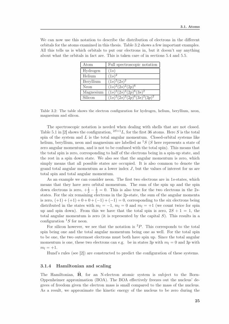
We can now use this notation to describe the distribution of electrons in the differentorbitals for the atoms examined in this thesis. Table 3.2 shows a few important examples.All this tells us is which orbitals to put our electrons in, but it doesn’t say anythingabout what the orbitals in fact are. This is taken care of in sections 5.4 and 5.5.
Atom Full spectroscopic notation
Hydrogen (1s)
Helium (1s)2
Beryllium (1s)2(2s)2
Neon (1s)2(2s)2(2p)6
Magnesium (1s)2(2s)2(2p)6(3s)2
Silicon (1s)2(2s)2(2p)6(3s)2(3p)2
Table 3.2: The table shows the electron configuration for hydrogen, helium, beryllium, neon,magnesium and silicon.
The spectroscopic notation is needed when dealing with shells that are not closed.Table 5.1 in [2] shows the configuration, 2S+1L, for the first 36 atoms. Here S is the totalspin of the system and L is the total angular momentum. Closed-orbital systems likehelium, beryllium, neon and magnesium are labelled as 1S (S here represents a state ofzero angular momentum, and is not to be confused with the total spin). This means thatthe total spin is zero, corresponding to half of the electrons being in a spin-up state, andthe rest in a spin down state. We also see that the angular momentum is zero, whichsimply means that all possible states are occupied. It is also common to denote thegrand total angular momentum as a lower index J , but the values of interest for us aretotal spin and total angular momentum.
As an example we can consider neon. The first two electrons are in 1s-states, whichmeans that they have zero orbital momentum. The sum of the spin up and the spindown electrons is zero, +1
2 − 12 = 0. This is also true for the two electrons in the 2s-
states. For the six remaining electrons in the 2p-state, the sum of the angular momentais zero, (+1) + (+1) + 0 + 0 + (−1) + (−1) = 0, corresponding to the six electrons beingdistributed in the states with ml = −1, ml = 0 and ml = +1 (we count twice for spinup and spin down). From this we have that the total spin is zero, 2S + 1 = 1, thetotal angular momentum is zero (it is represented by the capital S). This results in aconfiguration 1S for neon.
For silicon however, we see that the notation is 3P . This corresponds to the totalspin being one and the total angular momentum being one as well. For the total spinto be one, the two outermost electrons must both have spin up. Since the total angularmomentum is one, these two electrons can e.g. be in states 3p with ml = 0 and 3p withml = +1.
Hund’s rules (see [2]) are constructed to predict the configuration of these systems.
3.1.4 Hamiltonian and scaling
The Hamiltonian, H, for an N-electron atomic system is subject to the Born-Oppenheimer approximation (BOA). The BOA effectively freezes out the nucleus’ de-grees of freedom given the electron mass is small compared to the mass of the nucleus.As a result, we approximate the kinetic energy of the nucleus to be zero during the
25

Chapter 3. Many-particle Systems
calculations. The Hamiltonian consists of only the kinetic energy of electrons in addi-tion to the potential energy between electrons and the core, and between the electronsthemselves. The Born-Oppenheimer Hamiltonian is given as
H =
N∑
i
p2i
2me−
N∑
i
Ze2
4πǫ0ri+∑
i<j
e2
4πǫ0rij. (3.15)
The operator p is the kinetic energy operator, me is the electron mass, Z is the numberof protons in the nucleus (equal to the number of electrons in neutral atoms) and ǫ0the vacuum permittivity. The variables ri and rij represent the distances between anelectron and the nucleus and the distance between to different electrons respectively.
By substituting p with the quantum mechanical operator p = −i~∇, i being theimaginary unit and ~ Planck’s original constant divided by 2π, we get
H = − ~2
2me
N∑
i
∇2i −
N∑
i
Ze
4πǫ0ri+∑
i<j
e2
4πǫ0rij. (3.16)
It is more desireable to work with a scaled version of the Hamiltonian. By defining
r0 ≡ 4πǫo~2
mee2, (3.17)
and
Ω ≡ mee4
(4πǫ0~)2, (3.18)
we can write dimensionless variables such as H ′ = H/Ω, ∇′ = ∇/r0 and r′ = r/r0. Thefactors r0 in ∇′ comes from the factors d/dx = d/d(x′r0). By analyzing each term inEq. (3.15) and writing out the original variables in terms of constants r0 and Ω, and thedimensionless quantities r′ and H′ we get
H = H′Ω = − ~2
2mer20
N∑
i
(∇′i)
2 +e2
4πǫ0ro
N∑
i
1
r′i− Ze2
4πǫ0r0
∑
i<j
1
r′ij. (3.19)
By inserting Eqs. (3.17) and (3.18) into Eq. (3.19) we obtain
H′Ω = −Ω
2
N∑
i
(∇′i)
2 − Ω
N∑
i
Z
r′i+ Ω
∑
i<j
1
r′ij, (3.20)
which divided by Ω will give the final dimensionless Hamiltonian
H = −1
2
N∑
i
∇2i −
N∑
i
Z
ri+∑
i<j
1
rij. (3.21)
Now the energy will be measured in the units of Hartree, Eh, which converts as,1Eh = 2 · 13.6 eV. These are also called atomic units. We recognize the number 13, 6 asthe ground state energy of the hydrogen atom (see section 2.3.3).
26

3.2. Hartree-Fock Theory
3.2 Hartree-Fock Theory
A popular and well used many-particle method is the Hartree-Fock method. Hartree-Fock theory assumes the Born-Oppenheimer approximation and can be used to approx-imate the ground state energy and ground state wave function of a quantum manybody system. In Hartree-Fock theory we assume the wave function, Φ, to be a singleN -particle Slater determinant. A Hartree-Fock calculation will result in obtaining thesingle-particle wave functions which minimizes the energy. These wave functions canthen be used as optimized wave functions for a variational Monte Carlo machinery (seesection 4.4). The single particle orbitals for an atom are given as
ψnlmlsms = φnlml(r)χms(s), (3.22)
where ml is the projection of the quantum number l, given as merely m in section 3.1.3.The quantum number s represents the intrinsic spin of the electrons, which is s = 1/2.The quantum number ms now represents the two projection values an electron can have,namely ms = ±1/2. For a simple description, we label the single particle orbitals as
ψnlmlsms = ψα, (3.23)
with α containing all the quantum numbers to specify the orbital. The N -particle Slaterdeterminant is given as
Φ(r1, r2, . . . , rN , α, β, . . . , ν) =1√N !
∣∣∣∣∣∣∣∣∣
ψα(r1) ψα(r2) · · · ψα(rN )ψβ(r1) ψβ(r2) · · · ψβ(rN )
......
. . ....
ψν(r1) ψν(r2) · · · ψν(rN )
∣∣∣∣∣∣∣∣∣
. (3.24)
The Hamiltonian (see section 3.1.4) is given as
H = H1 + H2 =N∑
i=1
(−1
2∇2i −
Z
ri
)+∑
i<j
1
rij. (3.25)
or even as
H =
N∑
i=1
hi +∑
i<j
1
rij, (3.26)
with hi being the one-body Hamiltonian
hi = −1
2∇2i −
Z
ri. (3.27)
The variational principle (section 4.3) tells us that the ground state energy for ourHamiltonian, E0, is always less or equal to the expectation value of the Hamiltonianwith a chosen trial wave function, Φ. That is
E0 ≤ E[Φ] =
∫Φ∗HΦdτ, (3.28)
where the brackets in E[Φ] tells us that the expectation value is a functional, i.e. afunction of a function, here an integral-function. The label τ represents a shorthandnotation for dτ = dr1dr2 . . . drN . We also assume the trial function Φ is normalized
∫Φ∗Φdτ = 1. (3.29)
27

Chapter 3. Many-particle Systems
By introducing the so-called anti-symmetrization operator, A, and the Hartree-function,ΦH = ψα(r1)ψβ(r2) . . . ψν(rN ), we can write the Slater determinant (Eq. 3.24) morecompactly as
Φ(r1, r2, . . . , rN , α, β, . . . , ν) =√N !AΦH . (3.30)
The Hartree-function is as shown a simple product of the available single particles statesand the operator A is given as
A =1
N !
∑
P
(−)PP, (3.31)
with P being the permutation operator of two particles, and the sum spanning over allpossible permutations of two particles. The operators H1 and H2 themselves do notdepend on permutations and will commute with the anti-symmetrization operator A,namely
[H1,A] = [H2,A] = 0. (3.32)
The operator A also has the property
A = A2, (3.33)
which we can use in addition to Eq. (3.32) to show that
∫Φ∗H1Φdτ = N !
∫Φ∗HAH1AΦHdτ (3.34)
= N !
∫Φ∗HH1AΦHdτ. (3.35)
By using Eq. (3.30) and inserting the expression for H1 we arrive at
∫Φ∗H1Φdτ =
N∑
i=1
∑
P
(−)P∫
Φ∗H hiPΦHdτ. (3.36)
Orthogonality of the single-particle functions ensures us that we can remove the sumover P , as the integral will disappear when the two Hartree-Functions, Φ∗
H and ΦH
are permuted differently. As the operator hi is a single-particle operator, all factorsin ΦH except one, φµ(ri), will integrate out under orthogonality conditions, and theexpectation value of the H1-operator is written as
∫Φ∗H1Φdτ =
N∑
µ=1
∫ψ∗µ(ri)hiψµ(ri)dri. (3.37)
The two-body Hamiltonian, H2, can be treated similarly:
∫Φ∗H2Φdτ = N !
∫Φ∗HAH2AΦHdτ (3.38)
=
N∑
i<j=1
∑
P
(−)P∫
Φ∗H
1
rijPΦHdτ. (3.39)
28

3.2. Hartree-Fock Theory
In order to reduce this to a simpler form, we cannot use the same argument as for H1
for get rid of the P -sum, because of the form of the interaction, 1/rij . The permutationsof two electrons will not vanish and must be accounted for by writing
∫Φ∗H2Φdτ =
N∑
i<j=1
∫Φ∗H
1
rij(1 − Pij)ΦHdτ. (3.40)
Pij is the operator which permutes electrons i and j. However, by inspecting theparenthesis (1 − Pij) we can again take advantage of the orthogonality condition inorder to further simplify the expression:
∫Φ∗H2Φdτ =
1
2
N∑
µ=1
N∑
ν=1
[ ∫ψ∗µ(ri)ψ
∗ν(rj)
1
rijψµ(ri)ψν(rj)dridrj
−∫ψ∗µ(ri)ψ
∗ν(rj)
1
rijψµ(rj)ψν(ri)dridrj
]. (3.41)
The first term is the Hartree term, while the second term is called the Fock term.Alternatively they are called the direct and exchange terms. We see the exchange termhas permuted the particles i and j in the ΦH-function. The factor of 1/2 is due to thefact that we sum freely over µ and ν instead of using
∑i<j.
Combining the results from H1 and H2 you get the full Hartree-Fock energyfunctional
E[Φ] =
N∑
µ=1
∫ψ∗µ(ri)hiψµ(ri)dri+
1
2
N∑
µ
N∑
ν
[∫ψ∗µ(ri)ψ
∗ν(rj)
1
rijψµ(ri)ψν(rj)dridrj
−∫ψ∗µ(ri)ψ
∗ν(rj)
1
rijψν(ri)ψν(rj)dridrj
]
(3.42)
where now hi are the one body Hamiltonians, that is the sum of the kinetic energy andthe one-body interaction with the nucleus. The states ψµ and ψν are the Hartree-Fockorbitals which minimizes the energy when we solve the Hartree-Fock equations. UsingBra-Ket notation (see section 2.2), the energy functional can be written more compactlyas
E[Φ] =
N∑
µ=1
〈µ|h |µ〉 +1
2
N∑
µ=1
N∑
ν=1
[〈µν| 1
rij|µν〉 − 〈µν| 1
rij|νµ〉
]. (3.43)
3.2.1 Hartree-Fock equations
There are basically two approaches when it comes to minimizing the energy functionalin Eq. (3.43). The most straight forward, but a bit more demanding method is to varythe single particle orbitals. The other approach is to expand the single particle orbitalsin a well known basis as
ψa =∑
λ
Caλψλ, (3.44)
where now the ψλ are in a known orthogonal basis (e.g. hydrogen-like wave functions,harmonic oscillator functions etc.), and we vary the functions ψa with respect to theexpansion coefficients Caλ.
29

Chapter 3. Many-particle Systems
Varying the single particle wave functions
The background for these calculations are the principles of variational calculus asdescribed in section 18.4.1 in [9]. By introducing so-called Lagrangian multipliers wecan minimize a multivariable-variable functional with constraints. For this particularproblem, we introduce N2 such Lagrange multipliers, ǫµν . The variational equation(section 18.4.1 in [9]) for the energy functional in Eq. (3.42) is written as
δE −N∑
µ=1
N∑
ν=1
ǫµνδ
∫ψ∗µψν = 0. (3.45)
We still assume the wave functions are orthogonal, so the variational equation can bewritten
δE −N∑
µ=1
ǫµ
∫ψ∗µψµ = 0. (3.46)
The next step is to perform variation with respect to the single particle orbitals ψµ,which gives
N∑
µ
∫δψ∗
µhiψµdri +1
2
N∑
µ=1
N∑
ν=1
[∫δψ∗
µψ∗ν
1
rijψµψνdridrj −
∫δψ∗
µψ∗ν
1
rijψνψµdridrj
]
+
N∑
µ
∫ψ∗µhiδψµdri +
1
2
N∑
µ=1
N∑
ν=1
[∫ψ∗µψ
∗ν
1
rijδψµψνdridrj −
∫ψ∗µψ
∗ν
1
rijδψνψµdridrj
]
−N∑
µ=1
ǫµ
∫δψ∗
µψµdri −N∑
µ=1
ǫµ
∫ψ∗µδψµdri = 0. (3.47)
The variations δψ and δψ∗ are obviously not independent as they are only a complextransformation apart, but they can indeed be treated independently by replacing δψ bythe imaginary iδψ and correspondingly δψ∗ by iδψ∗. The terms depending on δψ andδψ∗ respectively can now be set equal to zero, yielding two independent sets of equations.By again combining them we will obtain the Hartree-Fock equations
[−1
2∇2i −
Z
ri+
N∑
ν=1
∫ψ∗ν(rj)
1
rijψ∗ν(rj)drj
]ψµ(ri)
−[N∑
ν=1
∫ψ∗ν(rj)
1
rijψ∗µ(rj)drj
]ψν(ri) = ǫµψµ(ri), (3.48)
where the integral∫drj also includes a sum over spin quantum numbers for electron j.
The first two terms in the first square bracket is the one-body Hamiltonian while thethird term is the direct term, representing a mean field of all the other electrons as seenby electron i. The term in the second square bracket is the exchange term, resultingfrom our antisymmetric wave function ansatz. This term also takes care of the so-calledself interaction from the first term by cancellation when i = j. We can now define thedirect and exchange operators
V dµ (ri) =
∫ψ∗µ(ri)
1
rijψµ(rj)drj , (3.49)
30

3.2. Hartree-Fock Theory
and
V exµ (ri)ψν(ri) =
(∫ψ∗µ
1
rijψν(rj)drj
)ψµ(ri). (3.50)
Then the Hartree-Fock equations may be written as
HHFi ψν(ri) = ǫνψν(ri), (3.51)
with
HHFi = hi +
N∑
µ=1
V dµ (ri) −
N∑
µ=1
V exµ (ri), (3.52)
as the Hartree-Fock matrix.In section 5.5, we will discuss the Roothaan-Hartree-Fock approach, which is based
on the method discussed in this section, with wave functions
ψ =∑
p
χpCp, (3.53)
where Cp(ξ) are some coefficients and χ are chosen to be the Slater type functions onthe form
χ(r) ∝ rn−1 exp(−ξr). (3.54)
Here ξ is some factor to be determined during the minimization. We see that we mustboth vary the parameters and the exponents. The results are given in section 5.5 andthe explicit expressions and results in [10].
Varying the coefficients
We see how the single particle functions in general, e.g. φ, are expressed as an expansionof known functions, ψ, on the form
φ =∑
i
Ciψi. (3.55)
In this section we will describe a method where we only vary the coefficients, and let theactual basis functions remain unchanged. This will in time give us a more time-efficientway to perform a Hartree-Fock calculation as we will show at a later stage.
The single particle basis functions are here denoted as ψλ, where λ = 1, 2, . . . andrepresents the full set of quantum numbers in order to describe a single particle orbital.Our new single particle orbitals will then be an expansion of these functions ψλ andwill have roman indices a = 1, 2, . . . to distinguish them from the chosen basis functionswith Greek indices. That is
ψa =∑
λ
Caλψλ, (3.56)
where Caλ are the expansion coefficients that will be varied. By using the Bra-Ketnotation we can introduce a more compact way to write the direct and exchange
terms from the Hartree-Fock energy functional. They are
〈µν|V |µν〉 =
∫ψ∗µ(ri)ψ
∗ν(rj)V (rij)ψµ(ri)ψν(rj)dridrj , (3.57)
and
〈µν|V |νµ〉 =
∫ψ∗µ(ri)ψ
∗ν(rj)V (rij)ψν(ri)ψµ(rj)dridrj , (3.58)
31

Chapter 3. Many-particle Systems
respectively. We have now only written V as a general potential instead of the explicitV = 1/rij .
The interaction does not change under a permutation of two particles, which meansthat
〈µν|V |µν〉 = 〈νµ|V |νµ〉 . (3.59)
This is also true for the general case
〈µν|V |σρ〉 = 〈νµ|V |ρσ〉 . (3.60)
We can have an even more compact notation by defining an antisymmetrized matrixelement
〈µν|V |µν〉AS = 〈µν|V |µν〉 − 〈µν|V |νµ〉 , (3.61)
or for the general case
〈µν|V |σρ〉AS = 〈µν|V |σρ〉 − 〈µν|V |ρσ〉 . (3.62)
The antisymmetrized matrix element has the following symmetry properties:
〈µν|V |σρ〉AS = −〈µν|V |ρσ〉AS = −〈νµ|V |σρ〉AS . (3.63)
It is also hermitian, which means
〈µν|V |σγ〉AS = 〈σγ|V |µν〉AS . (3.64)
Using these definitions we can have a short-hand notation for the expectation value ofthe H2 operator (see Eq. (3.41)
∫Φ∗H2Φdτ =
1
2
N∑
µ=1
N∑
ν=1
〈µν|V |µν〉AS . (3.65)
which in turn will give the full energy functional
E[Φ] =
N∑
µ=1
〈µ|h |µ〉 +1
2
N∑
µ=1
N∑
ν=1
〈µν|V |µν〉AS , (3.66)
similar to the one in Eq. (3.43).The above functional is valid for any choice of single particle functions, so by using
the new single particle orbitals introduced above in Eq. (3.56), and by now calling ourHartree-Fock Slater determinant, Ψ, we then have
E[Ψ] =N∑
a=1
〈a| h |a〉 +1
2
N∑
a=1
N∑
b=1
〈ab|V |ab〉AS . (3.67)
By inserting the expressions for ψa we will then have
E[Ψ] =N∑
a=1
∑
αβ
C∗aαCaβ 〈α|h |β〉 +
1
2
N∑
a=1
N∑
b=1
∑
αβγδ
C∗aαC
∗bβCaγCbδ 〈αβ| V |γδ〉AS . (3.68)
Similarly as for the previous case where we minimized with respect to the wave functionsthemselves, we now introduce N2 Lagrange multipliers. As a consequence of choosing
32

3.2. Hartree-Fock Theory
orthogonal basis functions, i.e. 〈α|β〉 = δα,β , where δx,y is the Kronecker delta function,the new basis functions are orthogonal, and we have
〈a|b〉 = δa,b =∑
αβ
C∗aαCaβ 〈α| |β〉 =
∑
α
C∗aαCaα. (3.69)
The functional to be minimized will now be
E[Ψ] −∑
a
ǫa∑
α
C∗aαCaα (3.70)
giving a variational equation
d
dC∗kλ
[
E[Ψ] −∑
a
ǫa∑
α
C∗aαCaα
]
= 0, (3.71)
where we have minimized with respect to some coefficient C∗kλ since C∗
kλ and Ckλ areindependent. Inserting the energy functional from Eq. (3.66) we will get
∑
β
Ckβ 〈λ|h|β〉 − ǫkCkλ+1
2
N∑
b=1
∑
β,γ,δ
C∗bβCkγCbδ 〈λβ|V |γδ〉AS
+1
2
N∑
a=1
∑
α,γ,δ
C∗aαCaγCkδ 〈αλ|V |γδ〉AS = 0 (3.72)
as
d
dCkλ
N∑
a=1
∑
α,β
C∗aαCaβ 〈α|h|β〉
=
N∑
a=1
∑
α,β
Caβ 〈α|h|β〉 δkaδλα (3.73)
=∑
β
Ckβ 〈λ|h|β〉 . (3.74)
In the last term in Eq. (3.72) we can use that 〈αλ|V |γδ〉AS = −〈λα|V |γδ〉AS =〈λα|V |δγ〉AS and change summation variable in both sums from b to a which gives
∑
β
Ckβ 〈λ|h|β〉 − ǫkCkλ +
N∑
a=1
∑
α,γ,δ
C∗aαCkγCaδ 〈λα|V |γδ〉AS = 0, (3.75)
or by using
hHFλγ = 〈λ|h|γ〉 +
N∑
a=1
∑
α,δ
C∗aαCaδ 〈λα|V |γδ〉AS ,
we can write the Hartree-Fock equations for this particular approach as∑
γ
hHFλγ Ckγ = ǫkCkλ. (3.76)
This is now a non-linear eigenvalue problem which can be solved by an iterative process,or a standard eigenvalue method. The advantage of this approach is the fact that wecan calculate the matrix elements 〈α| h |β〉 and 〈αβ| V |γδ〉 once and for all, since wedon’t change the basis functions, but only their coefficients. In the first approach, wherewe vary the actual wave functions, we have to calculate these matrix elements for eachiteration. When we just vary the coefficients, we can calculate the matrix elementsand store them in a table before we start the iterative process. This will lead to aquicker algorithm, but we will see that the method of varying both coefficients and basisfunctions actually produces the best results.
33


Chapter 4
Quantum Monte Carlo
Monte Carlo methods are designed to simulate a mathematical system, or in our case, aquantum mechanical system. By using random numbers, these methods are consideredstochastic, i.e. non-deterministic unlike other simulation techniques, such as Hartree
Fock, Coupled Cluster Theory and Configuration Interaction, ref. [11]. Monte Carlomethods can be used to simulate quantum mechanical systems, but are also well suitedfor calculating integrals, especially high-dimensional integrals. There are in fact severalQuantum Monte Carlo techniques such as Diffusion Monte Carlo, Green’s function
Monte Carlo and Variational Monte Carlo, see [3]. In this thesis we will focus onthe Variational Monte Carlo method.
The Quantum Monte Carlo calculations are so called ab initio methods, which arefirst principle calculations These methods have their basis on probability and statistics,and in order to get good expectation values and variances, the quantity in question mustbe sampled millions of times. Each such sample is called a Monte Carlo cycle, and canbe mistaken for being linked with the dynamics of the system. However, the systems wewill examine are stationary, meaning that they are time-independent systems.
To use the Quantum Monte Carlo technique, we will need a Probability DistributionFunction (PDF), P (x), to guide our sampling and which characterizes the system, withx being some set of variables, and of course a quantity to sample, in our case the energyof the system, E. The expectation value of the quantity of interest, e.g. an operator Q,will now be
〈Q〉 =
∫P (x)Qdx. (4.1)
We will see in section 4.4.1 that the operator we are looking for in our case will be thelocal energy operator
EL(R;α) =1
ψTHψT (R;α), (4.2)
where R is the set of all spatial variables, ψT a trial wave function since we don’t havethe exact solution Ψ (if we did, we wouldn’t have to go through all of this), and α a setof variational parameters which will be discussed in the following section.
Since the Monte Carlo method is a statistical method involving average values etc.,a certain degree of uncertainty and error will always occur. A method to minimize theerror estimate, the so-called blocking technique, will be discussed as a way to get theresults as correct as possible. In addition to this, we will discuss the Davidon-Fletcher-
Powell-algorithm (DFP), which is an improvement of the Conjugate Gradient Method(CGM), see [12]. DFP is a method which finds the minimum of a multivariable function.

Chapter 4. Quantum Monte Carlo
This chapter will also discuss the variational principle and the Metropolis algorithmfor the Variational Monte Carlo method. The Metropolis-Hastings algorithm will also bediscussed including importance sampling which will improve the method further, withmore relevant sample points.
4.1 Markov chains
A Markov chain is a way to model a system which evolves in time, and depends solelyon it’s previous state. We can consider a system that is described by its constituentshaving different probabilities to occupy some physical state. That is, the system isdescribed by a PDF, wj(t), at an instance t, where the index j indicates that the systemis discretized (for simplicity). We now have a transition probability, Wij, which givesus the probability for the system going from a state given by wj(t) to a state wi(t+ ǫ),where ǫ is a chosen time step. The relation between the PDF’s wi and wj will be
wi(t+ ǫ) =∑
j
Wijwj(t), (4.3)
where wi and Wij are probabilities and must fulfill
∑
i
wi(t) = 1, (4.4)
and ∑
i
Wij = 1. (4.5)
We can also write this as a matrix equation
w(t+ ǫ) = Ww(t). (4.6)
The equilibrium state of the system can be described by
w(∞) = Ww(∞), (4.7)
which implies a steady state, since the transition matrix now has no effect on the statevector, w. Eq. (4.7) now reads as an eigenvalue equation. By solving this equation,the eigenvectors would then be w1,w2,w3, . . . and so on, while the correspondingeigenvalues would be λ1, λ2, λ3, . . . etc. If the largest eigenvalue is λ1, viz.
λ1 > λ2, λ3, λ4, . . . , (4.8)
the steady state would then be w1, as its eigenvalue would cause this state to dominateas time progresses.
However, we do not know the form of the transition probability, Wij , and need a wayto examine the conditions at equilibrium. We start with the so-called Master equation,
dwi(t)
dt=∑
j
[W (j → i)wj −W (i→ j)wi] , (4.9)
which expresses the time rate of the PDF as a balance between state transitionalprobabilities from states j to i and from state i to states j. At equilibrium this time
36

4.2. Random numbers
derivative is zero, dw(teq)/dt = 0, implying that the sums of the transitions must beequal, namely ∑
j
W (j → i)wj =∑
j
W (i→ j)wi. (4.10)
By using Eq. (4.5) on the right-hand side of the equation, we get
wi =∑
j
W (j → i)wj . (4.11)
We do, however, need an even more stringent requirement to obtain the correct solutions,which is the so-called detailed balance principle:
W (j → i)wj = W (i→ j)wi, (4.12)
saying that the transition rate between any two states i and j must be equal as well.This gives the condition
wiwj
=W (j → i
W (i→ j). (4.13)
The detailed balance principle is imposed on the system to avoid cyclic solutions. Thisprinciple ensures us that once the most probable state is reached, the one correspondingto the lowest eigenvalue, the system will not traverse back to any state, correspondingto higher eigenvalues, see ref. [13].
A Markov chain must also comply with the ergodic principle, which has as a criterionthat a system should have a non-zero probability of visiting all possible states duringthe process (see [3]). A Markov chain does only depend on its previous step, and willfulfill this condition of ergodicity. The Metropolis algorithm (see section 4.4.1) is basedon a Markovian process and fulfills this condition of the ergodic principle.
Our physical system, an atom consisting of N electrons, is a system that can bedescribed by a PDF and which only depends on its previous system state. The PDFis here the absolute square of the wave function, namely |ψ|2. Since this describes aMarkov process, a wise choice would then be to use the Metropolis algorithm in orderto simulate the system.
4.2 Random numbers
A main component of a Monte Carlo calculation is the use of random numbers. Themost common random number distribution is the uniform distribution, which returns arandom number r between zero and one, that is
r ∈ (0, 1) . (4.14)
The name uniform (chapter 7.1 in [12]) tells us that every number between 0 and 1 couldbe returned with equal probability. Another much used distribution is the Gaussian, ornormal distribution (see chapter 7.3.4 in [12]).
As we saw in section 4.1, a Markov chain is a mathematical model which relies onlyon it’s previous step in the calculation. The true random numbers used to calculatei.e. new positions for particles etc., should be uncorrelated. In computers however, wecannot get true random numbers, and must therefore settle for so-called Pseudo-RandomNumber Generators (PRNG), where the numbers are correlated. Another problem with
37

Chapter 4. Quantum Monte Carlo
these number generators is that they have a certain period, and this sequence of pseudo-random numbers will repeat itself after completing a cycle of the sequence. However,the pseudo-random number generators we use have quite large periods, and we will notsuffer because of this.
4.3 The Variational Principle
The main target for us is to solve the time independent Schrödinger equation
HΨ = EΨ (4.15)
where H is the Hamiltonian, the operator representing the energy of the system, Ψthe quantum mechanical wave function, and E the total energy of the system. Thevariational principle tells us that for any given choice of trial wave function, ψT , thetotal energy
E =〈ψT | H |ψT 〉〈ψT |ψT 〉
(4.16)
will always be larger or equal to the true ground state energy, E0, for the chosenHamiltonian H,
E0 ≤ 〈ψT | H |ψT 〉〈ψT |ψT 〉
. (4.17)
To show this, we exploit the fact that H is Hermitian, and that the Hamiltonian willhave a set of exact eigenstates forming a complete basis set, |Ψi〉. Our trial function canthen be expanded as
〈ψT | =∑
i
ci |Ψi〉 , (4.18)
and the expectation value for H using the trial function ψT will be
E =〈ψT | H |ψT 〉〈ψT |ψT 〉
=
∑ij c
∗i cj 〈Ψi| H |Ψj〉∑ij c
∗i cj 〈Ψi|Ψj〉
=|ci|2Ei 〈Ψi|Ψi〉|ci|2 〈Ψi|Ψi〉
=
∑i |ci|2Ei∑i |ci|2
. (4.19)
The crucial point is to know that every excited state energy, Ei, is greater or equal tothe ground state energy, E0, that is
E =|ci|2Ei 〈Ψi|Ψi〉|ci|2 〈Ψi|Ψi〉
=
∑i |ci|2Ei∑i |ci|2
≥ |ci|2E0 〈Ψi|Ψi〉|ci|2 〈Ψi|Ψi〉
=
∑i |ci|2Ei∑i |ci|2
= E0. (4.20)
This inequality gives an equality when you find the true ground state wave function, Ψ0,that is
E0 = 〈Ψ0| H |Ψ0〉 . (4.21)
As our main goal is to approximate the ground state energy, this is the basis of ourcalculations. This gives us an idea to introduce variational parameters to our trial wavefunction in search for a good approximation. Instead of just having the wave functionsdepending on the spatial coordinates as ψT = ψT (x, y, z), we can write ψT as
ψT = ψT (x, y, z, α, β, . . . ). (4.22)
38

4.4. Variational Monte Carlo
Our goal is to find the minimum of functional E in Eq. (4.16), viz. the set of parametersthat gives the lowest energy when calculating E. A common approach in VMC is tooalso search for the minimum of the variance. A priori, we know that when the varianceis exactly zero, we have found the true ground state. However, as we have no knowledgeof the true form of the wave function, we must make an ansatz for it. This ansatz willin general not have a minimum for both the energy and the variance for the same setof parameters. As mentioned in [14], the most efficient wave function is found if weuse a linear combination of the parameters that minimize the energy and the variancerespectively.
In this work however, I have focused on finding the minimum of the energy only.
4.4 Variational Monte Carlo
The main exercise with the Variational Monte Carlo process for atoms is to move theparticles in the system guided by a probability distribution and sample the energy atthese states in order to calculate various expectation values (mainly 〈E〉 and 〈E2〉).In our case we have a known Hamiltonian, H, and a chosen many-particle trial wavefunction, ψT . The expectation value of the Hamiltonian is
〈H〉 =
∫dRψ∗
T (R;α)H(R)ψT (R;α)∫dRψ∗
T (R;α)ψT (R;α), (4.23)
where R = (R1,R2, . . . ,RN) are all the coordinates for the N particles, and α is theset of all the variational parameters in question. The general procedure will now be
1. Construct a trial wave function, ψT as a function of the N particles’ coordinatesand the chosen variational parameters
2. Calculate 〈H〉 using Eq. (4.23)
3. Vary the parameters according to some minimization technique
We will first focus on the second item in the list above, with a focus on the Metropolisalgorithm.
4.4.1 VMC and the simple Metropolis algorithm
We assume first that our trial wave function, ψT , is not normalized so the quantummechanical probability distribution is then given as
P (R;α) =|ψT (R;α)|2
∫|ψT (R;α)|2 dR
. (4.24)
Equation (4.24) gives the PDF for our system. We now define a new operator, calledthe local energy operator as
EL(R;α) =1
ψTHψT (R;α), (4.25)
and the expectation value of the local energy is given as
〈EL(α)〉 =
∫P (R;α)EL(R;α)dR. (4.26)
39

Chapter 4. Quantum Monte Carlo
The dimensionless Hamiltonian in section 3.1.4 is given as
H = −1
2
N∑
i
∇2i −
N∑
i
1
ri+∑
i<j
1
rij. (4.27)
Inserting the Hamiltonian from Eq. (4.27) into Eq. (4.25), the local energy operator willbe
EL =1
ψT (R, α)
−1
2
N∑
i
∇2i −
N∑
i
1
ri+∑
i<j
1
rij
ψT (R, α). (4.28)
By observing that the last two terms don’t affect the wave function in any way, we have
EL =1
ψT (R, α)
(−1
2
N∑
i
∇2i
)ψT (R, α) −
N∑
i
1
ri+∑
i<j
1
rij. (4.29)
This will be quantity we sample in each Monte Carlo cycle, following our PDF fromEq. (4.24). The more we improve the trial wave function the closer the expectationvalue of the local energy, 〈EL〉, gets to the exact energy E.
As we sample the local energy EL we also sample E2L in order to get 〈E2
L〉 for thevariance
σ2EL
= 〈E2L〉 − 〈EL〉2. (4.30)
We see from appendix B that we now can calculate the
〈EL〉 =1
n
n∑
k=1
EL(xk), (4.31)
where xk are the points at which the local energy is sampled, and n are the number ofsample points.
An important note is that in Metropolis algorithm only involves ratios betweenprobabilities, so the denominator in Eq. (4.24) actually never needs to be calculated.We will see this in the next section.
The Metropolis algorithm
The Metropolis algorithm uses ratios between probabilities to determine whether or nota chosen particle is to be moved to a proposed position or not. When an electron ismoved, the set of positions R change to positions R′. The ratio w = P (R′)/P (R) isnow the transition probability from the state with particles being in positions R to astate where particles are in positions R′. This ratio w will now be
w =
∣∣∣∣ψT (R′)
ψT (R)
∣∣∣∣2
. (4.32)
The Metropolis algorithm tells us that if
w > 1, (4.33)
we automatically accept the new positions. If w < 1, we compare w with a randomnumber r, with r ∈ (0, 1). If
r ≤ w, (4.34)
40

4.4. Variational Monte Carlo
we also accept the new positions. If neither of the two inequalities are true, the chosenelectron remains at its position before the proposed move. The most effective way touse this method is to move one particle at a time before running the tests for w.
We now have enough information to describe the elements needed to calculate theexpectation value for the local energy using the Metropolis algorithm. The specifics ofthe implementation will be discussed in the next chapter, but the following points stillshow how it’s done.
1. Set all electrons in random positions initially, that is a set of positions R
2. Start a Monte Carlo cycle and a loop over electrons
3. Calculate the new position,R′
i = Ri + s ∗ r,for electron i using a uniform random number, r and a finite stepsize, s. This willchange the entire set of positions from R to R.
4. Calculate the ratiow = |ψT (R′)/ψT (R)|2,
5. Use the checks in Eqs. (4.33) and (4.34) to decide whether to accept new positions,R = R′, or to stay in initial positions R.
6. If accepted, update positions
7. Repeat steps 3 through 6 for each electron
8. After looping over all particles, calculate the local energy and update 〈EL〉 and〈E2
L〉.
9. Repeat steps 3 through 8 for the chosen number of Monte Carlo cycles
The transition rules being used here is called a uniform symmetrical transition rule, andit is common to keep the acceptance ratio around 0.5 (this is achieved by choosing thestep length s ≈ 1). The acceptance ratio is the number of accepted steps divided bytotal number of particle moves. However, this simple Metropolis algorithm does notseem very efficient, due to the way the new positions are calculated. They depend solelyon the previous position and not on any guiding mechanism. In order to make thismethod more efficient, we introduce the Metropolis-Hastings algorithm with so-calledimportance sampling. With importance sampling we will get a much higher acceptanceratio since the calculation of new positions and the Metropolis-test will depend on thegradient of the wave function. Figure 4.1 shows a float chart of the Metropolis method.
4.4.2 Metropolis-Hastings algorithm and importance sampling
As an improvement to our Metropolis algorithm, we introduce the Metropolis-Hastingsalgorithm, which involves importance sampling. A new term that has to be implementedis the quantum force of the system:
F = 21
ψT∇ψT , (4.35)
A physical interpretation of the quantum force, and therefore a good reason to implementit, is that the gradient of the wavefunction tells us which direction the electrons are
41

Chapter 4. Quantum Monte Carlo
and start the loopChoose number of MC cycles
All electrons moved?
Reject move
and update expectation values
All MC cycles completed?
Divide expectation values by number of cycles
and end all loops
yes
no
no
yes
yes
no
Set all electrons in random positions and calculate
Accept move and set
Get a random number
Calculate
Is
andCalculate
random variable,
Move an electron using
where is step length and is a
and then the ratio
?
ψT (R)R
s r
ψT (R′)
R′ = R+ 2s(r − 12)
w = |ψT (R′)/ψT (R)|2
w ≥ r
R = R′
EL E2L
r ∈ 〈0, 1〉
r ∈ 〈0, 1〉
Figure 4.1: A float chart describing the Metropolis algorithm
42

4.4. Variational Monte Carlo
moving. If we rather use the quantum force to steer us in the direction of the electronmovement, rather than sampling random points around the nucleus, the points we samplewill be more relevant and therefore our acceptance ratio increases to about 0.8-0.9.Despite the fact that computing the quantum force will increase the calculation timefor each cycle, this will in time decrease our thermalization period, the period for thesystem to reach a most likely state. This will result in a more efficient algorithm.
Importance sampling
The one-dimensional diffusion equation is written as
∂P (x, t)
∂t= D
∂2P (x, t)
∂x2, (4.36)
and describes how the probability distribution, P , of a random walker evolves in time. Dis the diffusion constant (see chapter 14 in [9] or chapter 1 in [3]). The Green’s function
G(y, x, t) =1
(4πD∆t)3N/2exp
(−(y − x)2/4Dt
), (4.37)
is a general solution to the diffusion equation for a single walker which starts off atposition x at time t = 0. By using discrete time steps, it can be shown that a Markovprocess models a diffusion process, as the transition probability in a time step ∆t fromposition x to position y, G(y, x,∆t), only depends on the previous position, or state.The Fokker-Planck equation:
∂P
∂t= D
∂
∂x
(∂
∂x− F
)P (x, t), (4.38)
describes the time evolution of a PDF. As opposed to the diffusion equation, the Fokker-Planck equation also includes a drift term, F , yielding a solution given as
G(y, x,∆t) =1
(4πD∆t)3N/2exp
(−(y − x−D∆tF (x))2/4D∆t
). (4.39)
This is very similar to the solution of the diffusion equation but includes the drift term, orexternal force, F . This can be interpreted as a probability distribution of a single randomwalker with a drift force term starting off at position x at time t = 0([15]). This Green’sfunction serves as a transition probability for an electron when it is under influence ofthe drift term, F . This new propability must be multiplied with the probability fromEq. (4.24) and the ratio of probabilities from Eq. 4.32 is then replaced by the modifiedratio
w =G(x, y,∆t)|ψT (y)|2G(y, x,∆t)|ψT (x)|2 , (4.40)
or more explicitly
w =|ψT (y)|2|ψT (x)|2 exp
(−(y − x−D∆tF (x))2 − (x− y −D∆tF (y))2)
). (4.41)
The Langevin equation (see [3]) is a stochastic differential equation describing the dy-namics of random walkers as
∂x(t)
∂t= DF (x(t)) + η, (4.42)
43

Chapter 4. Quantum Monte Carlo
where η is a random variable following the uniform distribution between 0 and 1.Integrating this equation using the concepts of stochastic integration, will yield theequation
y = x+DF (x)∆t+ ξ√
∆t, (4.43)
where ξ now is a Gaussian distributed random variable and ∆t is a chosen timestep.This equation replaces Eq. (3) as the equation that calculates the new position for aparticle. We see that this depends on the drift term, the quantum force, F (x). Thisdrift term “pushes” the walkers in the direction of more probable states because thegradient of our PDF will point in the direction of higher values of probability.
By using the Fokker-Planck equation (where P is a time-dependent probabilitydensity),
∂P
∂t= D
∂
∂x
(∂
∂x− F
)P (x, t), (4.44)
and restraining a system to be in a stationary state, that is ∂P/∂t = 0, we find the formof F as
F (x) =1
P
dP
dx, (4.45)
or
F (r) =1
P∇P (4.46)
in three dimension, giving us a constraint for the form of the quantum force. Ourquantum mechanical system has a probability distribution given as
P (r) = |ψT (r)|2, (4.47)
and the quantum force of our system will be
F (x) = 21
ψT∇ψT . (4.48)
This algorithm will speed up the process as more important or relevant states are sampled(or visited in state space), hence the name, importance sampling.
Metropolis-Hastings algorithm
The Metropolis-Hastings algorithm can be summarized in the same way as for the simpleMetropolis algorithm:
1. Set all electrons in random positions as an initial point, x
2. Start a Monte Carlo cycle and a loop over electrons
3. Calculate the new position,
yi = xi +DF (x)∆t+ ξ√
∆t
for the chosen electron i using a Gaussian distributed number, ξ and a chosentimestep, ∆t
4. Calculate the quantum force for the new set of positions, y, and then the Green’sfunction
44

4.4. Variational Monte Carlo
5. Calculate the ratio w from equation Eq. (4.41)
6. Use the checks in Eqs. (4.33) and (4.34) to decide whether to accept new positions,y, or to stay in initial positions x
7. If accepted, update positions and quantum force
8. Repeat steps 3 through 7 for each electron
9. After looping over all particles, calculate the local energy and update 〈EL〉 and〈E2
L〉.
10. Repeat steps 3 through 9 for the chosen number of Monte Carlo cycles
Figure 4.2 shows a float chart of the Metropolis-Hastings algorithm. The detailedimplementation as a computer program will be discussed in the next chapter.
Both the simple Metropolis and the Metropolis-Hastings algorithms demand 4Nrandom numbers per Monte Carlo cycle, where N is the number of particles. Per particlemove, we need 3 normal distributed random numbers to make a move in each of thespatial dimensions. We also need one uniformly distributed random number for theMetropolis-test itself.
45

Chapter 4. Quantum Monte Carlo
and start the loopChoose number of MC cycles
All electrons moved?
Reject move
and update expectation values
All MC cycles completed?
Divide expectation values by number of cycles
and end all loops
no
no
yes
yes
no
Set all electrons in random positions
Is
andCalculate
?
a Gaussian random variable.
and calculate
Move an electron using
Calculate
and
yes
Accept move and setand
number
Get a Gaussian random
,
and
where is the quantum force, diff. constant
ψT (x) F (x)x
ψT (y)
y = x+DF (x)∆t+ ξ√
∆t
F (y)
F D
ξ
w = G(x,y,∆t)|(ψT (y)|2
G(y,x,∆t)|ψT (x)|2
w ≥ r
x = y
F (x) = F (y)
EL E2L
ξ
Figure 4.2: A float chart describing the Metropolis-Hastings algorithm
46

Chapter 5
Wave Functions
As the expectation values calculated with VMC depend on the chosen trial function,the results rely heavily on an educated guess. In this chapter we will examine the wavefunctions used for the Variational Monte Carlo method, and why they are good choices.This chapter will also introduce a correlation part, the Jastrow factor, to our trial wavefunction, since a pure Slater determinant is not enough to describe the inter-electroniccorrelations in an atomic system.
5.1 Cusp conditions and the Jastrow factor
The cusp conditions are constraints we get on the wave function when consideringour system when distances between an electron and the core and between the electronsthemselves become very small. The problems lie with the Coulomb force which dependson the inverse of the distance between charged particles. When these distances becomesmall, we need some way to cancel the divergences that occur.
5.1.1 Single particle cusp conditions
In order to find the cusp conditions for the single particle wave functions, we start byexamining the radial Schrödinger equation
− ~2
2m
(1
r2d
drr2d
dr− l(l + 1)
r2
)R(r) + V (r)R(r) = ER(r), (5.1)
where R(r) is the radial part of the full wave function. The dimensionless radial equationcan be written as
(d2
dρ2+
2
ρ
d
dρ+
2Z
ρ− l(l + 1)
ρ2+ 2E
)R(ρ) = 0, (5.2)
with Z being the nuclear charge of the core. We now introduce
R(ρ) =1
ρu(ρ) (5.3)
as our radial wave function. This will give the radial equation as
d2u(ρ)
dρ2+
2Z
ρu(ρ) − l(l + 1)
ρ2u(ρ) + 2Eu(ρ) = 0. (5.4)

Chapter 5. Wave Functions
As ρ approaches zero, the terms that dominate will be
d2u(ρ)
dρ2− l(l + 1)
ρ2u(ρ) = 0. (5.5)
The general solution of this differential equation is
u(ρ) = Cρl+1 +Dρ−l. (5.6)
As ρ−l will blow up as ρ approaches zero, the only physical solution we can have is then
u(ρ) ∼ ρl+1. (5.7)
In general we must assume that
R(ρ) = ρl+1γ(ρ), (5.8)
where γ(ρ) is just some radial dependence function of ρ with the constraint that γ(0) 6= 0.For the kinetic energy not to diverge, we also need
limρ→0
d2γ(ρ)
dρ2= Ω, (5.9)
where Ω is finite. The dimensionless radial equation is now
(d2
dρ2+
2
ρ
d
dρ+
2Z
ρ− l(l + 1)
ρ2+ 2E
)ρlγ(ρ) = 0, (5.10)
By finding the derivatives
d2
dρ2
[ρlγ(ρ)
]= (l − 1)lρl−2γ(ρ) + 2lρl−1dγ(ρ)
dρ+ ρl
d2γ(ρ)
dρ2, (5.11)
and2
ρ
d
dρ
[ρlγ(ρ)
]= 2lρl−2γ(ρ) + 2ρl−1 dγ(ρ)
dρ, (5.12)
and inserting them into Eq. (5.10) while taking the limit when ρ→ 0, we will get
γ(ρ)
[l(l + 1)
ρ2+
2Z
ρ− l(l + 1)
ρ2
]+dγ(ρ)
dρ
[2(l + 1)
ρ
]= 0 (5.13)
as the terms that dominate. The second derivative from Eq. (5.9) is finite, as well asthe term involving the energy E. By further simplification we will then have the cuspcondition as
1
γ(ρ)
dγ(ρ)
dρ= − Z
l+ 1, (5.14)
which indicates the exponential behavior a wave function must have. The solution ofequation Eq. (5.14) is
γ(ρ) ∼ e−Zρ/(l+1). (5.15)
The hydrogenic wave functions and the Roothan-Hartree-Fock orbitals both fulfill thecusp condition.
48

5.2. Rewriting the Slater determinant
5.1.2 Correlation cusp conditions
To see how the wave function should behave with respect to correlation, we consider thehelium system when the two electrons are very close, but far away from the core, that is,r1 6= 0, r2 6= 0 and r12 → 0. Now the electron-nucleus terms in the Hamiltonian will befinite, while the repulsive electron-electron potential and the kinetic energy of the twoelectrons will diverge. When using center of mass coordinates for electron 1 and 2, butneglecting the center of mass motion since r12 → 0, we will get a cusp condition also forthe correlation part by using much of the same derivations as in section 5.1.1. The cuspcondition for the two-particle part, R(r12), will then be
dR(r12)
dr12=
1
2(l + 1)R(r12), (5.16)
as given in [3] and [9].A correlation function that satisfies this cusp condition is the so-called Padé-Jastrow-
function given by the two-particle functions
f(rij) = exp
(rij
a(1 + βrij)
), (5.17)
where β is a variational parameter. The factor a is a result of whether the intrinsic spinsof particles i and j are parallel or not. That is
a =
4 if spins are parallel,
2 if spins are anti-parallel.(5.18)
The full Padé-Jastrow function, J , for a system of N electrons will then be
J =
N∏
i<j
f(rij) =
N∏
i<j
exp
(rij
a(1 + βrij)
), (5.19)
which also satisfies the cusp condition.
5.2 Rewriting the Slater determinant
A general Slater determinant for an N-electron system will take the form:
Φ(r1, r2, . . . , rN , α, β, . . . , ν) =1√N !
∣∣∣∣∣∣∣∣∣
ψα(r1) ψα(r2) · · · ψα(rN )ψβ(r1) ψβ(r2) · · · ψβ(rN )
......
. . ....
ψν(r1) ψν(r2) · · · ψν(rN )
∣∣∣∣∣∣∣∣∣
, (5.20)
where the ψ’s are the available single particle orbitals. We could examine this morespecifically by using the beryllium atom as an example. The Slater determinant forberyllium is written as
Φ(r1, r2, r3, r4, α, β, γ, δ) =1√4!
∣∣∣∣∣∣∣∣
ψα(r1) ψα(r2) ψα(r3) ψα(r4)ψβ(r1) ψβ(r2) ψβ(r3) ψβ(r4)ψγ(r1) ψγ(r2) ψγ(r3) ψγ(r4)ψδ(r1) ψδ(r2) ψδ(r3) ψδ(r4)
∣∣∣∣∣∣∣∣, (5.21)
49

Chapter 5. Wave Functions
with the quantum numbers representing different states as
|µ〉 = |n, l,ml, χ±〉 , (5.22)
with |α〉 = |1, 0, 0 ↑〉, |β〉 = |1, 0, 0 ↓〉, |γ〉 = |2, 0, 0 ↑〉 and |δ〉 = |2, 0, 0 ↓〉. The valuesχ± are given as χ+ =↑ and χ− =↓ (see section 2.1.2).
By writing out the determinant in Eq. (5.21) explicitly, we would get zero, as thespatial wave functions for both spin up and spin down states are identical, and all termswill cancel each other out. We could also try to rewrite the Slater determinant as aproduct of a spin up-Slater determinant and a spin down-Slater determinant as
Φ(r1, r2, r3, r4, α, β, γ, δ) = Det ↑ (1, 2)Det ↓ (3, 4) −Det ↑ (1, 3)Det ↓ (2, 4)
−Det ↑ (1, 4)Det ↓ (3, 2) +Det ↑ (2, 3)Det ↓ (1, 4) −Det ↑ (2, 4)Det ↓ (1, 3)
+Det ↑ (3, 4)Det ↓ (1, 2), (5.23)
where we have defined
Det ↑ (1, 2) =1√2
∣∣∣∣ψ100↑(r1) ψ100↑(r2)ψ200↑(r1) ψ200↑(r2)
∣∣∣∣ , (5.24)
as a spin up-determinant, and
Det ↓ (3, 4) =1√2
∣∣∣∣ψ100↓(r3) ψ100↓(r4)ψ200↓(r3) ψ200↓(r4)
∣∣∣∣ , (5.25)
as a spin down-determinant. However, writing out all these smaller determinants, willstill give zero, but the strategy of separating the Slater determinant in one spin up andone spin down determinant is still pursued. The Hamiltonian does not depend on spin,so we wish to avoid summation over spin variables. As described in [16], we can actuallyapproximate the Slater determinant for a variational approach with a plain product ofa spin up- and a spin down-Slater determinant
Φ(r1, r2, . . . , rN ) ∝ Det ↑ Det ↓, (5.26)
where the determinants Det ↑ and Det ↓ are (N/2)× (N/2)-matrices for even numberedelectron systems as examined in this project. We place the first N/2 electrons in thespin up determinant and the rest in the spin down determinant. This ansatz for thewave function is not antisymmetric under particle exchange as a wave function shouldbe, but it will give the same expectation value as the correct Slater determinant for sucha spin independent Hamiltonian.
5.3 Variational Monte Carlo wave function
By reviewing the last two sections we can write the full trial wave function for or MonteCarlo experiment. It can be written
ψT = Φ · J, (5.27)
where the Slater determinant Φ can be approximated by
Φ(r1, r2, . . . , rN ) ∝ Det ↑ Det ↓, (5.28)
50

5.4. Orbitals for VMC
and J is
J =N∏
i<j
exp
(rij
a(1 + βrij)
). (5.29)
For an N -particle system with M = N/2 possible spatial orbitals, the spin updeterminant, Det ↑, can be written
Det ↑ ∝
∣∣∣∣∣∣∣∣∣
ψ1↑(r1) ψ1↑(r2) · · · ψ1↑(rN/2)
ψ2↑(r1) ψ2↑(r2) · · · ψ2↑(rN/2)...
.... . .
...ψM↑(r1) ψM↑(r2) · · · ψM↑(rN/2)
∣∣∣∣∣∣∣∣∣
, (5.30)
while the spin down determinant can be written
Det ↓ ∝
∣∣∣∣∣∣∣∣∣
ψ1↓(rN/2+1) ψ1↓(rN/2+2) · · · ψ1↓(rN )
ψ2↓(rN/2+1) ψ2↓(rN/2+2) · · · ψ2↓(rN )...
.... . .
...ψM↓(rN/2+1) ψM↓(rN/2+2) · · · ψM↓(rN )
∣∣∣∣∣∣∣∣∣
. (5.31)
These are the expressions needed for our trial wave function. The next two sectionsdescribe the single particle orbitals, the ψ’s, we use in our Slater determinant.
5.4 Orbitals for VMC
In order to construct a trial Slater determinant for the Variational Monte Carlo method,our first choice is to use the hydrogenic single particle functions obtained when solvingthe Schrödinger equation for hydrogen. These functions comply with the cusp conditionsdescribed in section 5.1.1.
5.4.1 S-orbitals
An s-orbital is a spatial wave function with quantum number l = 0. Introducing thevariational parameter α, the s-orbitals needed for calculating up to at least silicon, withN = 14 electrons, are 1s, 2s and 3s. Here we only need the radial part of the wavefunctions because the constant angular parts factor out in the Metropolis algorithm (seesection 4.4.1). The spherical harmonics for l = 0 is
Y 00 =
(1
4π
)1/2
. (5.32)
We now don’t have to consider changing from spherical to Cartesian coordinates becausethe expression will remain the same using the simple relation r =
√x2 + y2 + z2. The
hydrogenic radial functions are found in table 4.7 in [2] where non-vanishing factors(cf.Metropolis algorithm) 1/a have been replaced by α.
The 1s wave function
For the 1s function we only need the exponential function
φ1s = e−rα, (5.33)
51

Chapter 5. Wave Functions
with the first derivative with respect to an arbitrary coordinate, xi, given as:
∂φ1s
∂xi= −αxi
re−αr. (5.34)
The Laplacian, ∇2 = ∂2
∂x2 + ∂2
∂y2+ ∂2
∂z2, needed for the kinetic energy is given as
∇2φ1s =α
r(αr − 2) e−αr. (5.35)
The 2s wave function
The 2s wave function is given by
φ2s =(1 − αr
2
)e−αr/2, (5.36)
with the first derivative with respect to. xi is
∂φ2s
∂xi=αxi2r
(2 − αr
2
)e−αr/2. (5.37)
The second derivative of the 2s function gives the Laplacian of the function:
∇2φ2s =α
4r
(5αr − α2r2
2− 8
)e−αr/2. (5.38)
The 3s wave function
The final s-function is the 3s wave function. It is
φ3s =
(1 − 2αr
3+
2α2r2
27
)e−αr/3. (5.39)
The first derivative is
∂φ3s
∂xi=
(−1 +
10αr
27− 2α2r2
81
)αxie
−αr/3, (5.40)
while the second derivative summed up in all three dimensions is
∇2φ3s =
(−2 +
13αr
9− 2α2r2
9+
2α3r3
243
)α
re−αr/3. (5.41)
5.4.2 P-orbitals
The p-orbitals are the single particle functions which have azimuthal quantum num-
ber l = 1. Now the allowed values for the magnetic quantum number arem = −l,−l + 1, . . . , l − 1, l, i.e. m = −1, 0, 1. This is only possible for functionswith quantum numbers n = 1, 2, 3, . . . . In this thesis we only need s- and p-orbitals.
The angular parts for any p-orbital in spherical coordinates are
Y 01 =
(3
4π
)1/2
cos θ, (5.42)
52

5.4. Orbitals for VMC
Y ±11 = ±
(3
8π
)1/2
sin θe±iϕ. (5.43)
In my program however, I am working with real wave functions and Cartesian coor-dinates. This is taken care of by introducing real solid harmonics, Slm, as described inref. [6]. The single particle wave functions, ψnlm, are written on a separable form withspherical coordinates as
ψ(r, θ, ϕ)nlm = Rnl(r)Ylm(θ, ϕ). (5.44)
These are general solutions of the one-electron system in a central symmetric potentialfield. Our radial functions are on the form Rnl(r) = rlRnl(r). The solid harmonics, Y,are related to the spherical harmonics by
Ylm(r, θ, ϕ) = rlYlm(θ, ϕ). (5.45)
We can then write the wave function as
ψ(r, θ, ϕ)nlm = Rnl(r)Ylm(θ, ϕ) = Rnl(r)Ylm(r, θ, ϕ). (5.46)
Now there is an r-dependence in the angular part. We will only need the real-valuedsolid harmonics, Slm, related to the solid harmonics by
Sl,0 =
√4π
2l + 1Yl,0, (5.47)
Sl,m = (−1)m√
8π
2l + 1Re Yl,m, (5.48)
and
Sl,−m = (−1)m√
8π
2l + 1Im Yl,m. (5.49)
The real solid harmonics needed for us are simply S1,1 = x, S1,0 = z and S1,−1 = y. Asmentioned earlier, the Metropolis algorithm will take care of any multiplicative factorsin front of the wave functions, so we only need to consider one single spatial variablefrom the angular part of the wave function.
The 2p wave function
The expression for the 2p wave function in spherical coordinates is proportional to
R21 ∝ re−αr/2. (5.50)
By reviewing Eq. (5.45) and using the results from the real solid harmonics, we see thefactor rl = r is replaced by a coordinate xi. That is, xi = x, y, z depending on thequantum number m. The general case is then
φ2p(m) = xi(m)e−αr/2. (5.51)
with xi(1) = x, xi(0) = z and xi(−1) = y.
53

Chapter 5. Wave Functions
The first derivative depends on whether the coordinate being differentiated withrespect to matches the coordinate xi of the wave function or not. If these are the same,e.g. m = 1 → xi = x, the first derivative is
∂φ2p
∂x=
(1 − αx2
2r
)e−αr/2
r. (5.52)
The expressions are analogous for y and z also.If these coordinates do not match, e.g. φ2p(1) = x exp−αr/2 and the derivative is
with respect to y, the expression is
∂φ2p(1)
∂y= −αxy
re−αr/2. (5.53)
As for the first derivative, the second derivative also depends on which coordinate wedifferentiate with respect to. If the coordinates are the same, e.g. m = 1 → xi = x, thesecond derivative is
∂2φ2p
∂x2=α
r
(x3
2r
(1
r+α
2
)− 3x
2
)e−αr/2, (5.54)
while for different coordinates, e.g. φ2p(1) = x exp−αr/2 and the second derivative
is with respect to y, the expression is
∂2φ2p(1)
∂y2=αx
2r3
(αry2
2− r2 + y2
)e−αr/2. (5.55)
The final Laplacian is a sum of Eqs. (5.54) and (5.55) depending on which l-state isbeing used.
The 3p wave function
The 3p radial wave function is proportional to
R31 ∝(1 − rα
6
)αre−αr/3. (5.56)
By using the real solid harmonics for the full single particle wave function, we get ourexpression for the 3p wave function;
φ3p(m) = xi(m)(1 − αr
6
)αe−αr/3, (5.57)
with xi(1) = x, xi(0) = z and xi(−1) = y. The first derivative when differentiatingwith respect to. to the same coordinate xi, e.g. x, is
∂φ3p(1)
∂x=
(−(1 − αr
6
)(α2x2
3r+ α
)− α2x2
6r
)e−αr/3, (5.58)
while for different coordinates, e.g. x and y, it is
∂φ3p(1)
∂y=
(−(1 − αr
6
) α2yx
3r− α2xy
6r
)e−αr/3, (5.59)
54

5.5. Roothaan-Hartree-Fock with Slater-type orbitals
and∂φ3p(1)
∂z=
(−(1 − αr
6
) α2zx
3r− α2zx
6r
)e−αr/3. (5.60)
The second derivative with respect to the coordinate from the solid harmonic, e.g. x,is
∂2φ3p(1)
∂x2=
((1 − αr
6
)( x2
3r2+αx2
9r− 1
)+αx2
9r+
x2
6r2− 1
2
)α2x
re−αr/3, (5.61)
while the second derivative with respect to a different coordinate is
∂2φ3p(1)
∂y2=
((1 − αr
6
)( y2
3r2+αy2
9r− 1
3
)+αy2
9r+
y2
6r2− 1
6
)α2x
re−αr/3, (5.62)
and
∂2φ3p(1)
∂z2=
((1 − αr
6
)( z2
3r2+αz2
9r− 1
3
)+αz2
9r+
z2
6r2− 1
6
)α2x
re−αr/3. (5.63)
By combining these we get the Laplacian of the wave function, ∇2φ3p(1). The expressionfor this particular single partice wave function is
∇2φ3p(1) =∂2φ3p(1)
∂x2+∂2φ3p(1)
∂y2+∂2φ3p(1)
∂z2. (5.64)
These are all the explicit expressions needed for the Slater determinant with hydrogen-like wave functions.
5.5 Roothaan-Hartree-Fock with Slater-type orbitals
Another approach for the single particle basis is to use the single particle wavefunctions obtained using the Hartree-Fock method discussed in section 3.2.1. The Slaterdeterminant is of the form
Φ =1√N !
∣∣∣∣∣∣∣∣∣
φ1(r1) φ1(r2) · · · φ1(rN )φ2(r1) φ2(r2) · · · φ2(rN )
......
. . ....
φN (r1) φN (r2) · · · φN (rN )
∣∣∣∣∣∣∣∣∣
, (5.65)
where the functions φ are the single particle states. The Roothaan-Hartree-Fockapproach (see [10]) is to choose Slater type orbitals (STO) as the basis functions inour wave function expansion. The STO are discussed in [6] and in [10]. In this work Ihave used the exact form from [10]. These are given as
φiλα =∑
p
ψpλαCiλp, (5.66)
where λ corresponds to quantum number l. The index i refers to the ith orbital ofsymmetry λ, and p to the pth orbital of symmetry λ. The index α corresponds toquantum number m. The Slater functions, ψ, are on the form
ψpλα(r, θ, ϕ) = Rλp(r)Yλα(θ, ϕ), (5.67)
55

Chapter 5. Wave Functions
whereRλp = [(2nλp)!]
−1/2(2ξλp)nλp+1/2 rnλp−1e−ξλpr, (5.68)
and Y are the normalized spherical harmonics. The solutions of this particular approachare given in appendix A, taken from [10].
By using the idea of real solid harmonics (see section 5.4) and the fact that all basisfunctions ψ in φ will have the same index α, hence the same spherical harmonics, wecan ignore the pre-factor from the spherical harmonics (see section 4.4.1). Now the basisfunctions ψ will go from the form
ψi = Nirn−1 exp(−ξr)Yλα, (5.69)
in spherical coordinates, to
ψi = Nixirn−2 exp(−ξr), (5.70)
in Cartesian coordinates, where the factor Ni is the normalization constant fromEq. (5.68). The results from helium, beryllium, neon, magnesium and silicon are listedin appendix A. As an example on how to construct the single particle orbitals from thetables in appendix A, I use the example given in [10]:
n,λ Exponent, ξ 1s exp.coeff. 2s exp.coeff. n,λ Exponent, ξ 2p exp.coeff.
1S 6.56657 0.19030 0.00754 2P 2.21734 0.215261S 4.24927 0.82091 −0.25055 2P 1.00551 0.840522S 1.41314 −0.00364 0.870992S 0.87564 0.00251 0.18515
Table 5.1: The table shows a possible solution for the boron atom.
Consider table 5.1 as a solution of the boron atom. Boron has five electronsdistributed as (1s)2(2s)2(2p). This means we need 1s-, 2s- and 2p-orbitals. The firstcolumn tells us how many and which s-type Slater functions the 1s- and 2s-orbitals forthe Slater determinant will consist of. In this case it will be two of each type. The secondcolumn gives us the factors, ξ, in the exponents of the exponential functions. These willbe the same for both 1s- and 2s, and will also contribute to the prefactors Ni. The thirdcolumn gives the coefficients for the 1s single particle orbital for the Slater determinant,while the fourth column gives the coefficients for the 2s single particle orbital. The singleparticle orbitals for 1s and 2s will then only differ by the constants in front of the Slaterfunctions (the ψ’s from Eq. (5.66)).
The fifth column indicates that there are only two basis functions needed to describethe p-orbital, namely the 2p single particle orbital, while the sixth and seventh give theexponents and 2p-coefficients respectively.
The single particle orbitals are given in table 5.1 as
φ(1s) = 0.19030ψ1 + 0.82091ψ2 − 0.00364ψ3 + 0.00251ψ4 (5.71)
φ(2s) = 0.00754ψ1 − 0.25055ψ2 + 0.87099ψ3 + 0.18515ψ4 (5.72)
φ(2p) = 0.21526ψ5 + 0.84052ψ6, (5.73)
56

5.5. Roothaan-Hartree-Fock with Slater-type orbitals
where now ψ1 and ψ2 are Slater functions of type 1s, ψ3 and ψ4 of type 2s, and ψ5 andψ6 Slater functions of type 2p. For larger atoms, the p-orbitals will be linear combina-tions of different p-type Slater functions. The s- and p-type Slater functions do not mixat any point, seen from Eq. (5.66).
The Slater functions themselves written in Cartesian coordinates are given as
ψ1 = N1r0 exp(−6.56657r), (5.74)
ψ2 = N2r0 exp(−4.24927r), (5.75)
ψ3 = N3r1 exp(−1.41314r), (5.76)
ψ4 = N4r1 exp(−0.87564r), (5.77)
ψ5 = N5xi exp(−2.21734r), (5.78)
ψ6 = N6xi exp(−1.00551r), (5.79)
where xi corresponds to either x,y or z as described in section 5.4.2, and the factors Ni
are the normalization factors from Eq. (5.68).
5.5.1 Derivatives of Slater type orbitals
The analytic expressions needed for the Slater type orbitals are of the form
ψ1s ∝ exp(−ar), (5.80)
ψ2s ∝ r exp(−ar), (5.81)
ψ3s ∝ r2 exp(−ar), (5.82)
ψ2p ∝ xi exp(−ar), (5.83)
ψ4p ∝ r2xi exp(−ar), (5.84)
where a is some exponent determined by the Roothan-Hartree-Fock calculations and xithe coordinate from the real solid harmonics. In order to calculate the quantum force(see section 4.4.2) and the kinetic energy we need both the first and second derivativesof the wave functions.
First derivatives
The s-orbitals have first derivatives proportional to
∂ψ1s
∂xi∝ −axi exp(−ar), (5.85)
∂ψ2s
∂xi∝ (1 − ar)
xir
exp(−ar), (5.86)
∂ψ3s
∂xi∝ (2xi − raxi) exp(−ar), (5.87)
while the 2p-orbitals are
∂ψ2p(x)
∂x∝(
1 − x2a
r
)exp(−ar), (5.88)
∂ψ2p(x)
∂y∝ −xya
rexp(−ar), (5.89)
57

Chapter 5. Wave Functions
where the parenthesis, (x), indicates which real solid harmonics the function dependson. Equations (5.88) and (5.89) are examples with the solid harmonics being the x-coordinate, and the derivatives with respect to x and then y (see the discussion in5.4.2). The 4p-orbitals are proportional to
∂ψ4p(x)
∂x∝(2x2 − r2 − rx2a
)exp(−ar), (5.90)
∂ψ4p(x)
∂y∝ (2xy − rxya) exp(−ar), (5.91)
Second derivatives
The Laplacian of the s-orbitals are on the form
∇2ψ1s ∝a
r(ar − 2) exp(−ar) (5.92)
∇2ψ2s ∝(
2
r+ a2r − 4a
)exp(−ar) (5.93)
∇2ψ3s ∝(6 − 6ar + a2r2
)exp(−ar), (5.94)
while the Laplacians of the 2p-orbitals consist of the second derivatives
∂2ψ2p(x)
∂x2∝ ax
r
(−3 +
x2
r2+x2a
r
)exp(−ar), (5.95)
∂2ψ2p(x)
∂y2∝ x
r
(y2
r2− 1 +
ay2
r
)exp(−ar). (5.96)
The 4p-orbitals have the second derivatives
∂2ψ4p(x)
∂x2∝ x
(6 − 3x2a
r+ 3ar + x2a2
)exp(−ar), (5.97)
∂2ψ4p(x)
∂y2∝ x
(2 − 3y2a
r− ar + a2y2
)exp(−ar). (5.98)
The expressions for ∂2ψ4p(y)/∂y2, ∂2ψ4p(z)/∂y
2 etc. are identical to the ones above andare used to construct e.g.
∇2ψ4p(x) =∂2ψ4p(x)
∂x2+∂2ψ4p(x)
∂y2+∂2ψ4p(x)
∂z2. (5.99)
All these expressions are needed for the implementation of the Slater determinant, thequantum force and the kinetic energy in our VMC calculation.
58

Part II
Implementation and results


Chapter 6
Implementation of the Variational
Monte Carlo Method
The Variational Monte Carlo method was implemented by writing a C++-based code.The first thing was to implement a brute force code to handle the helium atom, and whichcould easily be reduced to solve the simple hydrogen system, with only one atom andhence no inter-electron potentials. Brute force means here that there was no importancesampling, so the simple Metropolis algorithm (see figure 4.1) was used. The next stepwas to implement importance sampling, in order to make the sampling more efficient,and hopefully getting better results for both energy and variance. This would mean wehad to replace the simple Metropolis algorithm with the Metropolis-Hastings algorithm,which includes importance sampling.
However, the code was not efficient at this stage. By calculating the explicit wavefunction for each particle move, and using numerical derivatives, there was still room forimprovement. For larger systems like beryllium, neon etc., we would need to implementa more efficient wave function with closed-form expressions for the Slater determinantand its derivatives, using the definitions given in section 5.2, in addition to an efficientcomputation of the Jastrow factor. By doing this we could improve the efficiency ofeach Monte Carlo cycle, resulting in less computation time. If this optimization of thewave function was made general enough, and we included closed form expressions for thesingle particle wave functions and their derivatives, we could easily use the program tocalculate an approximation to the ground state energy for basically any even-numberedatom.
In this chapter I will describe the optimized version of the program, since this is ofmost interest, and the part that has taken the most time to develop. I will also focuson the Metropolis-Hastings algorithm and not the more simple Metropolis algorithm.
Initially, the code was developed using object-oriented programming (OOP), butcomplications and little programming experience prevented me from fully exploiting thestrengths of OOP. However, the main Monte Carlo machinery is built within a singleclass, so at least one can argue that this approach has left me with a little more organizedcode. I will therefore not emphasize on the code structure, but rather on the key pointsof importance for the calculations.
At the end of this chapter I will describe the blocking method used to calculate thetrue standard error of the data sets produced by the VMC code. I will also discuss away to estimate the true VMC results for ∆t = 0 in the Metropolis-Hastings algorithm(see sections 4.4.2 and 4.4.2). A brief discussion of parallel computing is also included.
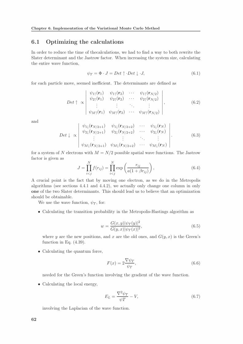
Chapter 6. Implementation of the Variational Monte Carlo Method
6.1 Optimizing the calculations
In order to reduce the time of thecalculations, we had to find a way to both rewrite theSlater determinant and the Jastrow factor. When increasing the system size, calculatingthe entire wave function,
ψT = Φ · J = Det ↑ ·Det ↓ ·J, (6.1)
for each particle move, seemed inefficient. The determinants are defined as
Det ↑ ∝
∣∣∣∣∣∣∣∣∣
ψ1↑(r1) ψ1↑(r2) · · · ψ1↑(rN/2)
ψ2↑(r1) ψ2↑(r2) · · · ψ2↑(rN/2)...
.... . .
...ψM↑(r1) ψM↑(r2) · · · ψM↑(rN/2)
∣∣∣∣∣∣∣∣∣
, (6.2)
and
Det ↓ ∝
∣∣∣∣∣∣∣∣∣
ψ1↓(rN/2+1) ψ1↓(rN/2+2) · · · ψ1↓(rN )
ψ2↓(rN/2+1) ψ2↓(rN/2+2) · · · ψ2↓(rN )...
.... . .
...ψM↓(rN/2+1) ψM↓(rN/2+2) · · · ψM↓(rN )
∣∣∣∣∣∣∣∣∣
. (6.3)
for a system of N electrons with M = N/2 possible spatial wave functions. The Jastrowfactor is given as
J =
N∏
i<j
f(rij) =
N∏
i<j
exp
(rij
a(1 + βrij)
), (6.4)
A crucial point is the fact that by moving one electron, as we do in the Metropolisalgorithms (see sections 4.4.1 and 4.4.2), we actually only change one column in onlyone of the two Slater determinants. This should lead us to believe that an optimizationshould be obtainable.
We use the wave function, ψT , for:
• Calculating the transition probability in the Metropolis-Hastings algorithm as
w =G(x, y)|ψT (y)|2G(y, x)|ψT (x)|2 , (6.5)
where y are the new positions, and x are the old ones, and G(y, x) is the Green’sfunction in Eq. (4.39).
• Calculating the quantum force,
F (x) = 2∇ψTψT
, (6.6)
needed for the Green’s function involving the gradient of the wave function.
• Calculating the local energy,
EL =∇2ψTψT
− V, (6.7)
involving the Laplacian of the wave function.
62

6.1. Optimizing the calculations
This means that we need to optimize the ratios Φ(rnew)/Φ(rold), ∇Φ(r)/Φ(r), ∇2Φ(r)/Φ(r),J(rnew)/J(rold), ∇J/J and ∇2J/J .
Since our wave function is on the form
ψT = Φ · J, (6.8)
the total expression for the gradient ratio will be
∇ψTψT
=∇Φ
Φ+
∇JJ. (6.9)
For the kinetic energy term in the local energy we will have to calculate the Laplacianof ψT , divided by ψT itself as
∇2ψTψT
=∇2Φ
Φ+
∇2J
J+
(∇Φ
Φ· ∇JJ
). (6.10)
6.1.1 Optimizing the ratio - ΨT (rnew)/ΨT (rold)
When optimizing the wave function part of the transition ratio, it’s a good idea to splitit into a correlation part, and a Slater determinant part. This means
R =ψT (rnew)
ψT (rold)= RSDRJ =
Φ(rnew)
Φ(rold)
J(rnew)
J(rold), (6.11)
where Φ is the Slater determinant, and J is the correlation part, the Jastrow factor. Inthis section I will label the positions of all particles before a particle move as rold, andthe set of particle positions after the move as rnew.
Slater determinant ratio - Φ(rnew)Φ(rold)
We start by defining the so-called Slater matrix, D, the matrix used to calculate the Slaterdeterminant, and its elements as Dij = φj(ri), where φj(ri) are electrons i occupyinga single particle state j. The inverse of the Slater matrix, D−1, is related to the Slaterdeterminant, Φ or just |D|, as
D−1 =adjD|D| , (6.12)
or as matrix elements as
D−1ij =
Cji|D| , (6.13)
where adjD is the so-called adjugate of a matrix. The adjugate of a matrix A is thetransposed of the co-factor matrix of A (indices are interchanged from Eq. (6.12) toEq. (6.13)). For the matrix D to be invertible, we must have D−1D = I, where I is theidentity matrix, or written out as
N∑
k=1
DikD−1kj = δij . (6.14)
Multiplying Eq. (6.13) with Dji from the left and summing over i, will give
N∑
i=1
DjiD−1ij =
∑Ni=1DjiCji|D| , (6.15)
63

Chapter 6. Implementation of the Variational Monte Carlo Method
resulting in
|D| =
N∑
i=1
DjiCji. (6.16)
We can now express the ratio between the new and old Slater determinants, RSD, as
RSD =
∑Nj=1Dij(r
new)Cij(rnew)
∑Nj=1Dij(rold)Cij(rold)
. (6.17)
When moving a particle i, only the i-th row of the Slater matrix changes, and thereforeonly the i-th row of the matrix of co-factors remains unchanged, which means
Cij(rnew) = Cij(r
old). (6.18)
Using Eq. (6.13) gives
RSD =
∑Nj=1Dij(r
new)Cij(rold)
∑Nj=1Dij(rold)Cij(rold)
=
∑Nj=1Dij(r
new)D−1ji (rold)
∑Nj=1Dij(rold)Dji(rold)
. (6.19)
This denominator will only give unity, so the ratio can be expressed as
RSD =
N∑
j=1
Dij(rnew)D−1
ji (rold) =
N∑
j=1
φj(rnewi )D−1
ji (rold). (6.20)
When only moving the i-th particle, we only need to calculate a dot product, φ(rnewi ) ·D−1i , where φ(rnewi ) is the vector
φ(rnewi ) = (φ1(rnewi ), φ2(r
newi ), ... , φN (rnewi )), (6.21)
and D−1i is the i-th column of the inverse matrix D−1 where the electron i is at the old
position. We also have splitted the determinants in two separate determinants, so we ac-tually only change one row in one of the Slater determinants when a particle i is moved.
The following code shows the function that calculates the ratio RSD:
double atom::getRatio(double **D_up, double **D_down, int i, double alpha, double
beta)
double ratio=0;
if(i<no_of_particles/2)
for(int j=0; j<no_of_particles/2; j++)
ratio += phi(r_new,alpha,beta,j,i)*D_up[j][i];
return ratio;
else
for(int j=0; j<no_of_particles/2; j++)
ratio += phi(r_new,alpha,beta,j,i)*D_down[j][i-no_of_particles/2];
return ratio;
64

6.1. Optimizing the calculations
Here the function phi(r,alpha,beta,j,i) calculates the single particle wave functionfor electron i in orbital j.
As described in [3] we can use an algorithm to update the inverse of the Slater matrixwithout calculating the entire Slater matrix again. After moving particle i, and if themove is accepted, we must for each column j 6= i calculate a quantity
Sj =
N∑
l=1
Dil(rnew)Dlj(r
old). (6.22)
The new elements of D−1 are as given on page 277 in [3]:
D−1kj (rnew) =
D−1kj (rold) − Sj
RSDD−1ki (rold) if j 6= i,
1RSD
D−1kj if j = i.
(6.23)
The following code shows how we first update the spin up determinant, and then thespin down determinant
void atom::update(double **D_up, double **D_down, int i, double ratio, double alpha,
double beta)
//SPIN UP ELECTRONS
if(i<no_of_particles/2)
for(int j=0; j<no_of_particles/2; j++)
if(j!=i)
for(int l=0; l<no_of_particles/2; l++)
s_j[j]+=phi(r_new,alpha,beta,l,i)*D_up[l][j];
for(int j=0; j<no_of_particles/2; j++)
if(j!=i)
for(int k=0; k<no_of_particles/2; k++)
D_up[k][j]=D_up[k][j]-s_j[j]*D_up[k][i]/ratio;
//i'th column, i=j
for(int k=0; k<no_of_particles/2; k++)
D_up[k][i]=D_up[k][i]/ratio;
//SPIN DOWN ELECTRONS
else
i=i-no_of_particles/2;//This is because the spin-down matrix have indices 0,1,....,
N/2
for(int j=0; j<no_of_particles/2; j++)
if(j!=i)
for(int l=0; l<no_of_particles/2; l++)
s_j[j]+=phi(r_new,alpha,beta,l,i+no_of_particles/2)*D_down[l][j];
for(int j=0; j<no_of_particles/2; j++)
if(j!=i)
for(int k=0; k<no_of_particles/2; k++)
D_down[k][j]=D_down[k][j]-s_j[j]*D_down[k][i]/ratio;
65

Chapter 6. Implementation of the Variational Monte Carlo Method
//i'th column, i=j
for(int k=0; k<no_of_particles/2; k++)
D_down[k][i]=D_down[k][i]/ratio;
i=i+no_of_particles/2;
Jastrow ratio - J(rnew)/J(rold)
We now have to find a functional way to store the inter-electron distances, or forsimplicity, the individual Jastrow functions,
gi,j = g(rij) = exp
(rij
a(1 + βrij)
), (6.24)
between the different electrons i and j, where a is given by
a =
4 if spins are parallel,
2 if spins are anti-parallel.(6.25)
From section 5.1.2, we have our Jastrow factor, J , on the form
J =∏
i<j
gi,j. (6.26)
A way to store these functions is to construct a matrix with elements above the diagonalas:
G =
· g1,2 g1,3 · · · g1,N· g2,3 · · · g2,N
· . . ....
· gN−1,N
. (6.27)
The Jastrow ratio, RJ is
RJ =J(rnew)
J(rold). (6.28)
From section 5.1.2, our Jastrow factor, J , is on the form
J =∏
i<j
gi,j =∏
i<j
exp fi,j, (6.29)
and when moving only particle k, only the elements with k as an index will change, thatis N − 1 elements. Because of our exponential form of the correlation part the ratio canbe written
J(rnew)
J(rold)= e∆J , (6.30)
where the intriguing part is ∆J , given as
∆J =
k−1∑
i=1
(fnewi,k − f oldi,k ) +
N∑
i=k+1
(fnewk,i − f oldk,i ), (6.31)
66

6.1. Optimizing the calculations
with the functions fij given as
fij =rij
a(1 + βrij). (6.32)
The following code shows the calculation of the Jastrow factor ratio:
double atom::getJastrowRatio(double** distance_old, double** distance_new,double beta)
for(int k=0; k<no_of_particles; k++)
for(int l=0; l<k; l++)
jastrowRatio += distance_new[l][k]-distance_old[l][k];
for(int k=0; k<no_of_particles; k++)
for(int l=k+1; l<no_of_particles; l++)
jastrowRatio += distance_new[l][k]-distance_old[l][k];
return jastrowRatio;
The two-dimensional arrays distance_new and distance_old have been calculatedusing:
void atom::getDistance(double** distance, double** r_old, double beta)
for(int k=0; k<no_of_particles; k++)
for(int l=k+1; l<no_of_particles; l++)
temp = diffR(r_old, k,l);
//spin up
if(((k < no_of_particles/2) && (l <no_of_particles/2)) || ((k>=no_of_particles/2
&& l>=no_of_particles/2)))
a=0.25;
distance[k][l] = a*temp/(1+beta*temp);
//spin down
else
a=0.5;
distance[k][l] = a*temp/(1+beta*temp);
We see that the names of the arrays are a bit misleading, as we actually store the valuesf(rij) (see Eq. (6.32)) and not rij themselves.
6.1.2 Derivative ratios
In order to optimize the calculations, we need to find optimized expressions for the ratios∇Φ/Φ, ∇2Φ/Φ, ∇J/J and ∇2J/J , as seen in Eqs. (6.9) and (6.10). This will lead to amore efficient evaluation of the quantum force and the kinetic energy.
Optimizing the ratios - ∇Φ/Φ and ∇2Φ/Φ
We use a similar procedure as in the previous section to get the explicit expressions forthe gradient and Laplacian of the Slater determinant. When differentiating with respect
67

Chapter 6. Implementation of the Variational Monte Carlo Method
to the coordinates of a single particle i, we will get
∇iΦ
Φ=
N∑
j=1
∇iDij(r)D−1ji (r) =
N∑
j=1
∇iφj(ri)D−1ji (r), (6.33)
for the gradient, remembering that the operator ∇ actually is a vector
∇ =∂
∂xı+
∂
∂y+
∂
∂zk, (6.34)
with ı, and k are the unit vectors for x-, y- and z- dimensions respectively.For the Laplacian-expression we will obtain
∇iΦ
Φ=
N∑
j=1
∇2iDij(r)D
−1ji (r) =
N∑
j=1
∇2iφj(ri)D
−1ji (r), (6.35)
where ∇2 is a scalar
∇2 =∂2
∂x2+
∂2
∂y2+
∂2
∂z2. (6.36)
We see that the expressions only rely on the elements from the inverse Slater matrix,D−1, and the closed form expressions for the derivatives of the single particle orbitals(see sections 5.4 and 5.5).
The following code shows the calculation of the ratio ∇2Φ/Φ in the local energy function:
//LAPLACE SLATER-DETERMINANT ANALYTIC
for(int i=0; i<no_of_particles; i++)
if(i<no_of_particles/2)
for(int j=0; j<no_of_particles/2; j++)
E_kinetic -= laplace_phi(r,alpha,beta,j,i)*D_up[j][i];
else
for(int j=0; j<no_of_particles/2; j++)
E_kinetic -= laplace_phi(r,alpha,beta,j,i)*D_down[j][i-no_of_particles/2];
The function laplace_phi(r,alpha,beta,j,i) simply returns the Laplacian of thesingle particle wave function where electron i is in orbital j.
Optimizing the ratios - ∇J/J and ∇2J/J
The first derivative results for the Padé-Jastrow function (as described in Eq. (6.26))are taken from chapter 19 in [9] and is for a single coordinate, x, for particle k, given by
1
J
∂J
∂xk=
k−1∑
i=1
1
gik
∂gik∂xk
+N∑
i=k+1
1
gki
∂gki∂xk
, (6.37)
where gij is some correlation function between two particles. We have
gij = exp f(rij) = exp
(rij
a(1 + βrij)
), (6.38)
68

6.1. Optimizing the calculations
a function of distances between the electrons. We now use the chain rule to get
∂gij∂xj
=∂gij∂rij
∂rij∂xj
=xj − xirij
∂gij∂rij
. (6.39)
The exponential form of gij also gives us
∂gij∂rij
= gij∂fij∂rij
, (6.40)
so that
1
J
∂J
∂xk=
k−1∑
i=1
∂fik∂xk
+
N∑
i=k+1
∂fki∂xk
. (6.41)
It is easy to show that∂fij∂rij
=1
a(1 + βrij)2, (6.42)
and combining these results we will get
1
J
∂J
∂xk=
k−1∑
i=1
xk − xiarik(1 + βrik)2
+
N∑
i=k+1
xk − xiarik(1 + βrik)2
, (6.43)
as the final result for the first derivative with respect to a chosen coordinate x, andparticle k. The quantum force for a given particle k in coordinate x,
F (xk) =2
J
∂J
∂xk= 2
(k−1∑
i=1
xk − xiarik(1 + βrik)2
+
N∑
i=k+1
xk − xiarik(1 + βrik)2
)
. (6.44)
The following code shows the calculation of the quantum force with the first part focusingon the Slater determinant part discussed in the previous section, while the second partfocuses on the correlation part of the quantum force (see Eq. (6.9)):
void atom::quantum_force(double**r,double**qm_force, double **D_up, double **D_down,
double alpha, double beta)
//SLATER PART
for(int p=0; p<no_of_particles; p++)
if(p<no_of_particles/2)
for(int q=0; q<dimension; q++)
for(int l=0; l<no_of_particles/2; l++)
qm_force[p][q] += 2*gradient_phi(r,alpha,q,l,p)*D_up[l][p];
else
for(int q=0; q<dimension; q++)
for(int l=0; l<no_of_particles/2; l++)
qm_force[p][q] += 2*gradient_phi(r,alpha,q,l,p)*D_down[l][p-no_of_particles/2];
//JASTROW PART
for(int p=0; p<no_of_particles; p++)
for(int q=0; q<dimension; q++)
for(int l=p+1; l<no_of_particles; l++)
69

Chapter 6. Implementation of the Variational Monte Carlo Method
qm_force[p][q] += 2*gradient_jastrow(r,p,l,q,beta);
for(int l=0; l<p; l++)
qm_force[p][q] += 2*gradient_jastrow(r,p,l,q,beta);
//end quantum_force
The function gradient_phi(r,alpha,q,l,p) returns the first derivative of the singleparticle orbital φl with respect to coordinate q of electron p.The function gradient_jastrow(r,p,l,q,beta)is given as
double atom::gradient_jastrow(double** r,int p, int l, int d, double beta)
if(((p < no_of_particles/2) && (l <no_of_particles/2)) || ((p>=no_of_particles/2 &&
l>=no_of_particles/2)))
a=0.25;//More efficient to multiply by 0.25 than to divide by 4
temp1 = diffR(r,p,l);
temp2 = 1+beta*temp1;
temp3 = r[p][d]-r[l][d];
return a*temp3/temp1/temp2/temp2;
else
a=0.5;//More efficient to multiply by 0.5 than to divide by 2
temp1 = diffR(r,p,l);
temp2 = 1+beta*temp1;
temp3 = r[p][d]-r[l][d];
return a*temp3/temp1/temp2/temp2;
The function diffR(r,p,l) simply returns the distance between electrons p and l.
For the second derivative, I refer to [9] where it is shown that for a correlation functionof our form
gij = exp fij, (6.45)
the full expression for the Laplacian of the correlation part can be written as
∇2J
J=
(∇JJ
)2
+
k−1∑
i=1
((d− 1)
rik
∂fik∂rik
+∂2fik∂r2ik
)
+N∑
i=k+1
((d− 1)
rki
∂fki∂rki
+∂2fki∂r2ki
), (6.46)
where the first term is just the dot product of the gradient (see the previous section)with itself, and d is the number of spatial dimensions, i.e. d = 3. We have the explicitexpression for the Padé-Jastrow correlation function
fij =rij
a(1 + βrij), (6.47)
where a is either 2 or 4 depending on the spins of particles i and j. The second derivativeof fij with respect to rij is now
∂2fij∂r2ij
= − 2β
a(1 + βrij)3, (6.48)
70

6.1. Optimizing the calculations
since the first derivative is∂fij∂rij
=1
a(1 + βrij)2, (6.49)
as in the previous section. Inserting Eqs. (6.49) and (6.48) into Eq. (6.46) will then give
∇2J
J=
(∇JJ
)2
+
k−1∑
i=1
(2
rik
1
a(1 + βrik)2− 2β
a(1 + βrik)3
)
+
N∑
i=k+1
(2
rki
1
a(1 + βrki)2− 2β
a(1 + βrki)3
), (6.50)
which can be reduced to
∇2J
J=
(∇JJ
)2
+
k−1∑
i=1
2
arik
1
(1 + βrik)3+
N∑
i=k+1
2
arki
1
(1 + βrki)3. (6.51)
In the local energy function we need to calculate the cross-term
∇Φ
Φ· ∇JJ, (6.52)
and ∇2J/J . The following code shows how I compute these quantities.
The Slater term, ∇Φ/Φ is computed as
//SLATER TERM:
for(int p=0; p<no_of_particles; p++)
if(p<no_of_particles/2)
for(int q=0; q<dimension; q++)
for(int l=0; l<no_of_particles/2; l++)
temp1[p][q] += gradient_phi(r,alpha,q,l,p)*D_up[l][p];
else
for(int q=0; q<dimension; q++)
for(int l=0; l<no_of_particles/2; l++)
temp1[p][q] += gradient_phi(r,alpha,q,l,p)*D_down[l][p-no_of_particles/2];
The following code shows how I compute the Jastrow term, ∇J/J , using the gradient_jastrow-functions explained previously.
//JASTROW TERM
for(int p=0; p<no_of_particles; p++)
for(int q=0; q<dimension; q++)
for(int l=p+1; l<no_of_particles; l++)
temp2[p][q] += gradient_jastrow(r,p,l,q,beta);
for(int l=0; l<p; l++)
temp2[p][q] += gradient_jastrow(r,p,l,q,beta);
71

Chapter 6. Implementation of the Variational Monte Carlo Method
We can now compute the cross-term by a simply dot product calculation using thefollowing code:
for(int p=0; p<no_of_particles; p++)
for(int q=0; q<dimension; q++)
tempE += temp1[p][q]*temp2[p][q];
The functions gradient_jastrow(...) and gradient_phi(...) have been explainedearlier. The array temp2[p][q] now contains the ratio ∇J/J and is used to calculatethe ratio ∇2J/J as given in Eq. (6.51). The code for this equation is:
//Gradient ratio squared:
for(int p=0; p<no_of_particles; p++)
for(int q=0; q<dimension; q++)
tempE2 += temp2[p][q]*temp2[p][q];
//Second term, involving df/dx and d^2f/dx^2
for(int p=0; p<no_of_particles; p++)
for (int k = 0; k < no_of_particles; k++)
if ( k != p)
if(((p < no_of_particles/2) && (k <no_of_particles/2)) || ((p>=no_of_particles/2 &&
k>=no_of_particles/2)))
a=0.25;
tempE3 += 2*a/diffR(r,p,k)/pow((1+beta*diffR(r,p,k)),3);
else
a=0.5;
tempE3 += 2*a/diffR(r,p,k)/pow((1+beta*diffR(r,p,k)),3);
We now have all the pieces to calculate the local energy with E_kinetic, tempE,tempE2and tempE3. We only need to multiply the different term by scalar factors, and calculatethe potential energy. The following code shows this.
//KINETIC ENERGY
E_kinetic -= 2*tempE;
E_kinetic -= tempE2;
E_kinetic -= tempE3;
E_kinetic *= 0.5;
//POTENTIAL ENERGY Coulomb potential
//electron-proton-interaction
for(int i=0; i<no_of_particles; i++)
r_single_particle=0;
for(int j=0; j<dimension; j++)
r_single_particle += r[i][j]*r[i][j];//r^2=x^2+y^2+z^2
E_potential -=charge/sqrt(r_single_particle);
//electron-electron-interaction
for(int i=0; i<no_of_particles-1; i++)
for(int j=i+1; j<no_of_particles; j++)
r_12=0;
72

6.2. Implementation of Metropolis-Hastings algorithm
for(int k=0; k<dimension; k++)
r_12 +=(r[i][k]-r[j][k])*(r[i][k]-r[j][k]);
E_potential +=1/sqrt(r_12);
//*/
E_local = E_potential + E_kinetic;
return E_local;
6.2 Implementation of Metropolis-Hastings algorithm
We can now use the results from the previous sections to show how the Metropolis-Hastings algorithm is implemented. This algorithm is discussed in section 4.4.2, andfigure 4.2 sums up the main points quite nicely.
After calculating the initial positions for the electrons, the inverse spin-up and -downSlater matrices and the quantum force F, I start the first Monte Carlo cycle and movethe first electron as
for(int j=0; j<dimension; j++)
r_new[i][j]=r_old[i][j]+D*time_step*qm_force_old[i][j]
+gaussian_deviate(&idum)*sqrt(time_step)
where the function gaussian_deviate returns a normal distributed random number. Ithen calculate the distances between the electrons to find both the Slater- and Jastrow-ratios for the full ratio of probabilities, ψT (rnew)/ψT (rold) as
//SETTING UP THE DISTANCE MATRIX
getDistance(distance_new, r_new, beta);
//SLATER DETERMINANT RATIO
ratio = getRatio(D_up, D_down, i, alpha, beta);
jastrowRatio = getJastrowRatio(distance_old, distance_new, beta);
jastrowRatio = exp(jastrowRatio);
The next point is to update the inverse Slater matrices, and then calculate the quantumforce for the Green’s function in the Metropolis-Hastings test:
//temporary update for quantum force
update(temp_up, temp_down, i, ratio, alpha, beta);
quantum_force(r_new, qm_force_new, temp_up, temp_down, alpha, beta);
//IMPORTANCE SAMPLING
double greensfunction = 0.0;
for(int k=0; k<no_of_particles; k++)
for(int j=0; j < dimension; j++)
greensfunction += 0.5*(qm_force_old[k][j]+qm_force_new[k][j])*
(D*time_step*0.5*(qm_force_old[k][j]-qm_force_new[k][j])
-r_new[k][j]+r_old[k][j]);
greensfunction = exp(greensfunction);
I use temporary arrays in case the Metropolis-Hastings test does not accept the particlemove. The test itself is implemented as
73

Chapter 6. Implementation of the Variational Monte Carlo Method
//METROPOLIS TEST
if(ran1(&idum)<= greensfunction*ratio*ratio*jastrowRatio*jastrowRatio)
for(int k=0; k<no_of_particles; k++)
for(int j=0; j<dimension; j++)
r_old[k][j]=r_new[k][j];
qm_force_old[k][j] = qm_force_new[k][j];
//UPDATE INVERSE SLATER MATRICES
for(int m=0; m<no_of_particles/2; m++)
for(int n=0; n<no_of_particles/2; n++)
D_up[m][n]=temp_up[m][n];
D_down[m][n]=temp_down[m][n];
//UPDATE THE DISTANCE MATRIX
for(int m=0; m<no_of_particles; m++)
for(int n=0; n<no_of_particles; n++)
distance_old[m][n]=distance_new[m][n];
//end metropolis test
The random number generator ran1 is taken from [12]. If now all particles for the cyclehave been moved, we can go on to sample the local energy for the expectation values〈EL〉 and 〈E2
L〉:delta_E = local_energy(r_old, D_up, D_down, alpha, beta);
energy +=delta_E;
energy2 +=delta_E*delta_E;
At the end of the Monte Carlo loop, we then divide the expectation values by the numberof Monte Carlo cycles we have performed.
Furthermore, an important note must be made regarding the calculation of the localenergy. At the beginning of the simulation, the system will in general not be in itsmost probable state. By reviewing section 4.1, we see that a system must evolve beforereaching its largest eigenvalue, corresponding to the most probable state. As a resultof this, we must include some thermalization cycles before we start sampling the localenergy. As seen in the algorithm, we initialize the system in random positions. Ifwe perform a certain number of Monte Carlo cycles before we start sampling the localenergy, the system will hopefully be in its most probable state when we actually do startsampling the energy. This will improve our results, since we will calculate the energywhere the PDF has greater values, leading to more efficient calculations.
The number of thermalization cycles is not known a priori, and must be dealt withexperimentally. In this thesis we found that by using 200, 000 thermalization cycles, wewill safely start sampling the energy when the system has reached its most probablestate, even for large systems.
6.3 Blocking
The simulation of physical systems using Monte Carlo methods, involve pseudo-randomnumbers and will produce correlated results. That is, as the pseudo-random numbersthemselves will show correlated behavior, functions evaluated with respect to variables
74

6.3. Blocking
dependent on these pseudo-random numbers will become correlated as well. As discussedin appendix B, the statistical error for set of correlated stochastic values is given by
err2X =1
nCov(x), (6.53)
while for uncorrelated values this will reduce to
err2X =1
nVar(x) =
1
n2
n∑
k=1
(xk − xn)2. (6.54)
As given in appendix B, we can write the error for correlated cases as
err2X =τ
nVar(x), (6.55)
where τ is the autocorrelation time
τ = 1 + 2
n−1∑
d=1
κd, (6.56)
describing the correlation between measurements. However, calculating κd, as given inEqs. (B.34) and (B.35), will be rather time consuming.
By using the blocking technique, or ’data bunching’, as described in [17] and [18],we actually have a way to make the measurements ’uncorrelated’. By grouping thedata in equally sized blocks, and treating the mean, or sample mean, of each block as ameasurement, we can find an error estimate by merely plotting the error as a functionof block size as if the data were uncorrelated.
Suppose we have 1000 measurements in our sample. We can then divide these valuesinto 10 blocks with 100 measurements in each block. Furthermore, we calculate themean in each block, and treat them as our measurements. Then we calculate the erroras if the data were uncorrelated using Eq. (6.54), where the block means are our xk’sand n = 10. The total sample mean,
xn =1
n
n∑
k=1
xk, (6.57)
will of course be identical whether we calculate it directly, that is for block sizes equal1 and n equal total number of measurements, or if we group them into blocks.
The blocking method tells us that for block sizes smaller than the correlation time,the distance between correlated measurements, calculating the error using Eq. (6.54)will underestimate the error. When the block size is larger than the correlation time,the measurements are no longer correlated, and the error will no longer be affected byvarying the block size. This becomes apparent as there will be a clear plateau whenthe data becomes uncorrelated. When the error reaches the plateau we have found anestimate for the true error,
A possible problem with relying on blocking is if the plateau is reached at a pointwhere the number of blocks is too small to accurately estimate the variance. In thisthesis we are lucky enough for that not to occur.
75

Chapter 6. Implementation of the Variational Monte Carlo Method
6.4 Time step extrapolation
By applying the Metropolis-Hastings algorithm, which introduces concepts and quan-tities from diffusion and random walk theory (see section 4.4.2), we are forced to dealwith a time step, ∆t, which for our practical calculations must be non-zero. We canunderstand this by inspecting the equation we use in the program for proposing a movefor an electron,
y = x+DF (x)∆t+ ξ√
∆t, (6.58)
where y is the proposed new position, x is the old position, D is the diffusion constant,F (x) is the quantum force (see section 4.4.2) and ξ is normal distributed random variable.By having ∆t = 0, the electrons would never move according to this model. However,our system is stationary, which means that we must have ∆t = 0 in order to simulatethe system correctly.
As done for the Diffusion Monte Carlo calculations (see e.g. [3]) by Sarsa in [19], itis possible to extrapolate towards ∆t = 0 by plotting results for non-zero ∆t and fittinga curve to the data plot.
In this work we have used a linear fitting which also accommodates for the standarderror of the data. This fitting model is based on the method in chapter 15.4 in [12], andcan both estimate the energy for ∆t = 0 and the standard error for ∆t = 0.
6.5 Parallel computing
In this program I have also implemented the possibility of running the code in parallel.This gives us the opportunity to run the code on several nodes simultaneously in orderto obtain more samples than just one node would give us in the same space of time.
A Monte Carlo calculation is especially easy to program in parallel. We can run theprogram separately on different nodes with a thermalization period that ensures us wehave reached the most probable state on all nodes. Furthermore, we can simply collectthe individual mean values from all the nodes into one common mean value, as if theindividual mean values were individual measurements (see section B in appendix B).
In this work I use the Titan cluster for large parallel jobs, such as variation ofsilicon, magnesium etc. The Titan computer cluster is described on its homepagehttp://hpc.uio.no.
76

Chapter 7
Hartree-Fock implementation
The Hartree-Fock method (HF) is discussed in section 3.2, and the results supply a greatimprovement to the single particle wave functions. Using HF, we find the optimal singleparticle wave functions (SPWF) for our chosen basis functions. By using the optimalSPWF, we no longer have to vary the Slater determinant in a VMC calculation, andcan consentrate on finding the minimum by varying the parameter(s) in the Jastrowfunction. As an example, I have implemented Hartree-Fock for the Beryllium atomusing the method of varying coefficients (see section 3.2.1). The basis functions are herechosen to be the hydrogen-like s-orbitals.
As seen in section 3.2.1, in order to get our single particle solutions
ψa =∑
λ
Caλφλ, (7.1)
we have to solve the Hartree-Fock equations
∑
γ
hHFλγ Ckγ = ǫkCkλ, (7.2)
where hHFλγ is
hHFλγ = 〈λ|h|γ〉 +
N∑
a=1
∑
α,δ
C∗aαCaδ 〈λα|V |γδ〉AS . (7.3)
We see how the coefficients Ckγ are involved on both sides of the equation, and thereforeleading to an non-linear eigenvalue problem.
7.1 Interaction matrix elements
As mentioned in section 3.2.1, this particular Hartree-Fock approach gives us theadvantage of computing the matrix elements 〈λα|V |γδ〉 once and for all. We havechosen the hydrogenic s-waves as the basis functions φλ from Eq. (7.1).
The interaction is given by the Coulomb force between the electrons, and the matrixelements are given by
〈λα|V |γδ〉 =
∫r21dr1
∫r22dr2R
∗nα0(r1)R
∗nβ0(r2)
1
r<Rnγ0(r1)Rnδ0(r2), (7.4)

Chapter 7. Hartree-Fock implementation
This is the direct term of the interaction piece. By calling the innermost integral overr2 for I,
I =
∫r22dr2Rnβ0(r2)
1
r<Rnδ0(r2),
we can split this up into two pieces. One where r2 < r1 and r< = r1 and one wherer2 > r1 with r< = r2, giving
I =
∫ r1
0r22dr2Rnβ0(r2)
1
r1Rnδ0(r2) +
∫ ∞
r1
r2dr2Rnβ0(r2)Rnδ0(r2),
The matrix element 〈λα|V |γδ〉 can then be written as
〈λα|V |γδ〉 =
∫ ∞
0r21dr1Rnα0(r1)Rnγ0(r1)
[∫ r1
0r22dr2Rnβ0(r2)
1
r1Rnδ0(r2)
+
∫ ∞
r1
r2dr2Rnβ0(r2)Rnδ0(r2)
]
. (7.5)
The exchange term 〈λα|V |δγ〉 can be written the same way only by exchanging δ ↔ γwhich gives
〈λα|V |δγ〉 =
∫ ∞
0r21dr1Rnα0(r1)Rnδ0(r1)
[∫ r1
0r22dr2Rnβ0(r2)
1
r1Rnγ0(r2)
+
∫ ∞
r1
r2dr2Rnβ0(r2)Rnγ0(r2)
](7.6)
In the equations above the functions Rn0 are defined by the radial part of the s-states,as
Rn0 =
(2Z
n
)3/2√
1
2n2L1n−1
(2Zr
n
)exp
(−Zrn
), (7.7)
with L1n−1
(2Zrn
)being the generalized Laguerre polynomials.
7.2 Algorithm and HF results
The Hartree-Fock program calculates the energy and optimized single particle wavefunctions to plug into the VMC machinery. We see from equation 7.2 that we aredealing with an eigenvalue problem. However, as the hHF -matrix depends on the matrixelements of C, we have a non-linear problem, and must use an iterative self-consistencyapproach.
• The first thing to do is to choose the number basis functions we wish to expandthe functions ψ in Eq. (7.1) with.
• We then calculate the matrix elements from Eq. (7.5). The elements were storedin a 4-dimensional array, and each integral was calculated using Gauss-Legendre-quadrature. One should really use Gauss-Laguerre to match the interval, but theGauss-Legendre approach seemed to work well.
78

7.2. Algorithm and HF results
• The next step is to start the iteration process. The first thing we need is an ansatzfor the C-matrix and we choose the identity matrix, corresponding to our new basisfunctions just being the old hydrogen s-waves. We then calculate the hHF -matrixfrom Eq. (7.3) which we then diagonalize using library C++-functions. We nowput the eigenvectors corresponding to the 4 lowest eigenvalues in the 4 first rowsas we only deal with Beryllium. We can now calculate the energy, and use themodified diagonalized matrix as the C-matrix for next the iteration.
• When the energy difference between two iterations is low enough (determined bya preset tolerance ∼ 10−6) we stop the iterations and we have reached a desiredset of coefficients for the new basis.
Table 7.1 shows the Hartree-Fock energy results for different number of s-waves includedin the wave function expansion. It also shows the number of iterations needed forthe energy difference between two succeeding iterations to be smaller than the chosentolerance. We see from table 7.1 that the ground state energy for 15 s-waves producesapproximately the same result as for 10 and 7 basis functions, but is improved in the5th digit. The table also presents the exact result as given in [20]. [20]
We can compare the best Hartree-Fock result when only varying coefficients, E =−14.5185 Eh, with the results from appendix A, E = −14.573021 Eh, where Slater-typeorbitals have been used. If we compare these with the exact result, E0 = −14.6674 Eh,it can lead us to believe that the Slater-type orbitals in the Roothaan-Hartree-Fockapproach are a better choice for improving the VMC calculations.
In section 6.5.2 in [6], an argument is given for not using hydrogenic functions asbasis functions for larger many-body atomic systems. They do not constitute a completeset by themselves, since the hydrogenic functions only describe bound states, and willnot describe the unbound continuum states needed for a complete set. They also spreadout quickly and become diffuse because of the 1/n-factors in the polynomials and theexponentials. The Slater-type orbitals have a more compact exponential radial form,and we will avoid the problems involving diffuseness and the completeness of the basisset.
HF basis functions Energy Iterations
2 -13.7159 2
3 -14.5082 9
4 -14.5115 10
5 -14.5141 11
7 -14.5165 10
10 -14.5178 11
15 -14.5185 10
Exact -14.6674 -
Table 7.1: The table shows results from different runs with different number of basis functionsin addition to the exact result. Energies are given in the Hartree unit.
79


Chapter 8
VMC Results
In this chapter I will present the results produced by the Variational Monte Carlo code.The first part shows the variational plots for both sets of single particle orbitals, thatmeans both hydrogen-like and Roothaan-Hartree-Fock orbitals. The next sections willbe dedicated to finding the optimal parameters using the DFP-algorithm. The thirdpart will present results of the time step extrapolation discussed in section 6.4 for thefinely tuned parameter(s) produced by the DFP method. These results will also includethe error estimates computed by the blocking method. The final part will compare theextrapolated results with calculations from [3] and [4].
All calculations are performed by the VMC code with the Metropolis-Hastingsalgorithm which includes importance sampling. There is a possibility that the minimumenergy is found using different variational parameters for different time steps whenanalyzing the same system. However, by doing a simple check for helium, I could notfind any significant difference for time steps ∆t = 0.05 and ∆t = 0.01. I then assumethat the optimal parameters give the minimum in energy for all time steps within areasonable range. Unless something else is stated, all results are calculated with timestep ∆t = 0.05.
8.1 Validation runs
In order to confirm that the Slater determinant is working properly, it is necessary totest the code. In most cases this means comparing the computed results with someclosed form- or analytic expressions. For the hydrogen-like orbitals, I have comparedwith the closed form hydrogen energy solutions, while the Slater-type orbitals have beencompared with the Roothaan-Hartree-Fock calculations (ref. [10]).
8.1.1 Hydrogen-like orbitals
To validate the Slater determinant with hydrogenic single particle orbitals, I run theprogram with no electron interaction. In this case this means using a pure Slaterdeterminant, without the Jastrow factor, as the trial wave function. If we also neglectthe electron-electron interaction energies, we can compare our results with the analyticresults obtained using hydrogenic wave functions.
A hydrogen-like atom, is any atom with charge Z and only one electron. For thissystem the energy is given as
ENI = −Z2
2
1
n2, (8.1)

Chapter 8. VMC Results
where n is the principle quantum number of the orbital the single electron is occupying,ψnlm (see chapter 6.5.2 in ref. [6]).
For non-interacting atomic systems, we can use the hydrogen results to get a closedform expression for the non-interacting energy, ENI . Since the electrons are non-interacting we can just add the energies of the orbitals as
ENI = −Z2
2
N∑
i=1
1
n2i
, (8.2)
where Z is the charge of the nucleus, N is the number of electrons, and ni is the prin-cipal quantum number for the state occupied by electron i. The energy is in units ofHartree. Table 8.1 shows how the electrons for our systems of interest are distributedin the different energy orbitals.
Atom Spectroscopic notation
Hydrogen (1s)
Helium (1s)2
Beryllium (1s)2(2s)2
Neon (1s)2(2s)2(2p)6
Magnesium (1s)2(2s)2(2p)6(3s)2
Silicon (1s)2(2s)2(2p)6(3s)2(3p)2
Table 8.1: The table shows the electron configuration for hydrogen, helium, beryllium, neon,magnesium and silicon.
As an example we can calculate the analytic non-interacting helium energy as
ENI(He) = −22
2
(1
12+
1
12
)= −4. (8.3)
By running the non-interacting version of the program for helium with, we get the exactenergy
E = −4. (8.4)
Table 8.2 shows that the exact energies calculated using Eq. (8.2) and the VMC resultsare identical for all atoms of interest. It is safe to say that the orbitals and the Slaterdeterminant have been implemented correctly. By running a sufficient number of MonteCarlo cycles (≈ 108), the variance will reduce to
σ2E = 10−5 − 10−6 (8.5)
for all such non-interacting systems.
8.1.2 Slater-type orbitals - Hartree Fock results
To validate the Slater-type orbitals (STO) found by using Hartree-Fock in ref. [10], Iran the code with STO but no Jastrow factor. Then I could compare the computedenergies with the energy results from ref. [10]. Table 8.3 shows this. We see how theenergies correspond quite nicely for the smaller systems, while the deviations increase
82

8.2. Variational plots
Atom ENI E
Helium −4.00 −4.00
Beryllium −20.00 −20.00
Neon −200.00 −200.00
Magnesium −304.00 −304.00
Silicon −435.56 −435.56
Table 8.2: The table shows the analytic results, ENI , the computed ground state energies, E,number of Monte Carlo cycles and the variance, σ2
E. The energy results are in units of Hartree.
slightly for larger systems. A variational Monte Carlo process should in theory reproducethe Hartree-Fock energy when using the corresponding Hartree-Fock orbitals. We couldhave performed a time step extrapolation to hopefully get even closer to the Hartree-Fock energies, but the results in table 8.3 make us quite confident that the Slater-typeorbitals form the Roothaan-Hartree-Fock calculations have been implemented correctly.
As an example I time extrapolated the results for neon, and got the value E =−128.55, which is in very good accordance with the HF energy from table 8.3.
Atom EHF E MC cycles σ2E
Helium −2.8616799 −2.8617823 3 · 107 0.57097060
Beryllium −14.573021 −14.573862 3 · 107 2.9477341
Neon −128.54705 −128.81981 1 · 108 31.003216
Magnesium −199.61461 −199.84100 1 · 108 41.645320
Silicon −288.85431 −289.11902 5 · 108 58.958016
Table 8.3: The table shows the Roothaan-Hartree-Fock results, EHF (see appendix A andref. [10]), compared with the computed energies using the Roothaan STO, E, number of MonteCarlo cycles and the variance, σ2
E. The energy results are in units of Hartree.
8.2 Variational plots
This section presents the plots of the variational runs for the different systems. Forthe hydrogen-like orbitals in section 8.2.1, the plots will be two-dimensional since thetotal wave function consists of two variational parameters. The parameters are α in theSlater determinant and β from the Jastrow function. For VMC calculations using theSlater-type orbitals presented in section 5.5, the plots will only be one-dimensional, sincethe single particle orbitals have already been optimized by the Roothaan-Hartree-Fockmethod. The variational parameter, β, comes from the Jastrow function.
8.2.1 Hydrogen-like orbitals
Figures 8.2, 8.3, 8.4, 8.5 and 8.6 show the variational results for helium, beryllium,neon, magnesium and silicon respectively. For the different variational calculations Ihave used between 10 and 100 million samples per parameter-set depending on thesize of the system (smaller systems demand less computational time and we can moreeasily compute smoother plots). However, the main goal with these plots is to find the
83

Chapter 8. VMC Results
0.10.2
0.30.4
0.50.6
1.51.6
1.71.8
1.92
−2.9
−2.85
−2.8
−2.75
−2.7
−2.65
β
Helium variational plot, 100 million samples
α
Exp
ecta
tion
valu
e of
ene
rgy,
<E
>
Figure 8.1: A typical variational plot. This plot shows the results for helium with 100 millionsamples. The energies are in units of Hartree.
1.5 1.55 1.6 1.65 1.7 1.75 1.8 1.85 1.9 1.95 2−2.9
−2.85
−2.8
−2.75
−2.7
−2.65Helium variational plot, 100 million samples
α
Exp
ecta
tion
valu
e of
ene
rgy,
<E
>
0.1 0.15 0.2 0.25 0.3 0.35 0.4 0.45 0.5 0.55 0.6−2.9
−2.85
−2.8
−2.75
−2.7
−2.65Helium variational plot, 100 million samples
β
Exp
ecta
tion
valu
e of
ene
rgy,
<E
>
Figure 8.2: The figures show a variational plot of the helium ground state energy with 100million samples using hydrogen-like orbitals. The figure on the left shows the variation of the αparameter, while the figure on the right shows the variation of the β parameter. The energiesare in units of Hartree.
84

8.2. Variational plots
3.5 3.55 3.6 3.65 3.7 3.75 3.8 3.85 3.9 3.95 4−14.5
−14.4
−14.3
−14.2
−14.1
−14
−13.9
−13.8Beryllium variational plot, 100 million samples
α
Exp
ecta
tion
valu
e of
ene
rgy,
<E
>
0 0.05 0.1 0.15 0.2 0.25 0.3 0.35 0.4 0.45 0.5−14.5
−14.4
−14.3
−14.2
−14.1
−14
−13.9
−13.8Beryllium variational plot, 100 million samples
β
Exp
ecta
tion
valu
e of
ene
rgy,
<E
>
Figure 8.3: The figures show a variational plot of the beryllium ground state energy with 100million samples using hydrogen-like orbitals. The figure on the left shows the variation of the αparameter, while the figure on the right shows the variation of the β parameter. The energiesare in units of Hartree.
9 9.1 9.2 9.3 9.4 9.5 9.6 9.7 9.8 9.9 10−128
−127.5
−127
−126.5
−126
−125.5
−125
−124.5
−124
−123.5Neon variational plot, 30 million samples
α
Exp
ecta
tion
valu
e of
ene
rgy,
<E
>
0.1 0.15 0.2 0.25 0.3 0.35 0.4 0.45 0.5 0.55 0.6−128
−127.5
−127
−126.5
−126
−125.5
−125
−124.5
−124
−123.5Neon variational plot, 30 million samples
β
Exp
ecta
tion
valu
e of
ene
rgy,
<E
>
Figure 8.4: The figures show a variational plot of the neon ground state energy with 30 millionsamples using hydrogen-like orbitals. The figure on the left shows the variation of the αparameter, while the figure on the right shows the variation of the β parameter. The energiesare in units of Hartree.
85

Chapter 8. VMC Results
10.5 10.6 10.7 10.8 10.9 11 11.1 11.2 11.3 11.4 11.5−202
−200
−198
−196
−194
−192
−190
−188Magnesium variational plot, 10 million samples
α
Exp
ecta
tion
valu
e of
ene
rgy,
<E
>
0 0.1 0.2 0.3 0.4 0.5 0.6 0.7 0.8 0.9 1−202
−200
−198
−196
−194
−192
−190
−188Magnesium variational plot, 10 million samples
βE
xpec
tatio
n va
lue
of e
nerg
y, <
E>
Figure 8.5: The figures show a variational plot of the magnesium ground state energy with 10million samples using hydrogen-like orbitals. The figure on the left shows the variation of the αparameter, while the figure on the right shows the variation of the β parameter. The energiesare in units of Hartree.
12.5 12.6 12.7 12.8 12.9 13 13.1 13.2 13.3 13.4 13.5−294
−292
−290
−288
−286
−284
−282
−280Silicon variational plot, 10 million samples
α
Exp
ecta
tion
valu
e of
ene
rgy,
<E
>
0 0.1 0.2 0.3 0.4 0.5 0.6 0.7 0.8 0.9 1−294
−292
−290
−288
−286
−284
−282
−280Silicon variational plot, 10 million samples
β
Exp
ecta
tion
valu
e of
ene
rgy,
<E
>
Figure 8.6: The figures show a variational plot of the silicon ground state energy with 10million samples using hydrogen-like orbitals. The figure on the left shows the variation of the αparameter, while the figure on the right shows the variation of the β parameter. The energiesare in units of Hartree.
86

8.2. Variational plots
whereabouts of the optimal parameters, and we are not concerned about precise energymeasurements. The plots does not precise optimal parameters, but by merely lookingat them, and where the energy has its minimum, we should be able to find very goodinitial values for the DFP-method (see appendix C). The DFP-method will hopefullysupply us with even better optimal parameters using initial values from table 8.4.
Atom α β MC cycles E
Helium 1.85 0.35 108 ≈ −2.89
Beryllium 3.90 0.12 108 ≈ −14.49
Neon 9.20 0.50 3 · 107 ≈ −127.7
Magnesium 10.8 0.40 107 ≈ −200
Silicon 12.6 0.50 107 ≈ −292
Table 8.4: The table shows the apparent optimal parameters from the variational Monte Carloplots. It also shows the number of Monte Carlo cycles and the approximate energy for theparameter set. The energies are in units of Hartree.
Table 8.4 shows the results for the variational parameters obtained by inspectingfigures 8.2, 8.3, 8.4, 8.5 and 8.6. Some plots are very flat, e.g. the magnesium plot withrespect to the α-parameter (see figure 8.5), and it is hard to determine the minimum byjust inspecting the plots.
We also see that the silicon plot is difficult to read as a function of the α-parameter(see figure 8.6). It seems as though the minimum lies at about α = 12.6, but this couldbe a local minimum since the plot does not show results for α-values less than 12.5.However, as we will see in section 8.3.1, the DFP-algorithm finds a minimum that lieswithin the plotted area.
To obtain smoother plots for both silicon and magnesium, I would have needed moresamples, hence more computational time at the end of this work. These large paralleljobs tended to crash due to an error in the MPI (Message Passing Interface) systemat Titan. When running the exact same code at a local computer, the program nevercrashed. However, the amount of computational time needed to get a smooth variationalplot of such large systems would be very large on a local computer. Due to these timelimitations and parallel jobs crashing at the Titan cluster (http://hpc.uio.no), I wasnot able to plot the silicon energy for parameter values lower than α = 12.5. Again,as mentioned in the previous paragraph, the DFP method does return a minimum forα-values larger than 12.5, so the range of the plot will not be a problem.
8.2.2 Slater-type orbitals - Hartree Fock results
In this case, the trial wave function is reduced to a one-parameter function, since theSlater determinant has already been optimized by the Hartree-Fock method. Whenpresenting the results, I will also include the variance plots to show that the parametersfor minimum in the energy and minimum in the variance in general do not coincide. Sincewe have chosen the DFP method to search for the parameter that gives a minimum inthe energy, this parameter value is the one we choose for further calculations.
Figures 8.7, 8.8, 8.9, 8.10 and 8.11 show the variation in the β parameter both forenergy and variance for helium, beryllium, neon, magnesium and silicon respectively. Wesee that the minimum in energy and variance does not occur for the same β parameter.Especially the magnesium and silicon plots (figures 8.10 and 8.11) show this behavior,
87

Chapter 8. VMC Results
with the minimum of variance not even being within the parameter interval we haveplotted.
Again, the time limitation does not allow us to get perfectly smooth plots for largersystems, but the plots still supply us with good information concerning the parameterthat gives a minimum in energy.
0.2 0.4 0.6 0.8 1 1.2 1.4 1.6 1.8 2−2.89
−2.885
−2.88
−2.875
−2.87
−2.865
−2.86
−2.855
−2.85
−2.845Helium variational plot, 150 million samples
β
Exp
ecta
tion
valu
e of
ene
rgy,
<E
>
0.2 0.4 0.6 0.8 1 1.2 1.4 1.6 1.8 20.04
0.06
0.08
0.1
0.12
0.14
0.16Helium variational plot, 150 million samples
β
Var
ianc
e, σ
2
Figure 8.7: The figures show a variational plot of the helium ground state energy with 150million samples using Slater type orbitals. The figure on the left shows the energy variation ofthe β parameter, while the figure on the right shows the variance variation of the β parameter.The energy results are in units of Hartree.
1 1.2 1.4 1.6 1.8 2 2.2
−14.61
−14.609
−14.608
−14.607
−14.606
−14.605
−14.604
−14.603
−14.602
Beryllium variational plot, 150 million samples
β
Exp
ecta
tion
valu
e of
ene
rgy,
<E
>
1 1.2 1.4 1.6 1.8 2 2.2
0.33
0.34
0.35
0.36
0.37
0.38
0.39
0.4
0.41
0.42
Beryllium variational plot, 150 million samples
β
Var
ianc
e, σ
2
Figure 8.8: The figures show a variational plot of the beryllium ground state energy with 150million samples using Slater type orbitals. The figure on the left shows the energy variation ofthe β parameter, while the figure on the right shows the variance variation of the β parameter.The energy results are in units of Hartree.
8.3 Optimal parameters with DFP
This section presents the results we get when using the minimization algorithm discussedin appendix C. The values in table 8.5 and 8.6 are average results of different DFP
88

8.3. Optimal parameters with DFP
2.5 3 3.5 4 4.5 5 5.5 6 6.5 7
−129.02
−129
−128.98
−128.96
−128.94
−128.92
−128.9Neon variational plot, 10 million samples
β
Exp
ecta
tion
valu
e of
ene
rgy,
<E
>
2.5 3 3.5 4 4.5 5 5.5 6 6.5 76
6.5
7
7.5
8
8.5Neon variational plot, 10 million samples
β
Var
ianc
e, σ
2
Figure 8.9: The figures show a variational plot of the neon ground state energy with 10 millionsamples using Slater type orbitals. The figure on the left shows the energy variation of the βparameter, while the figure on the right shows the variance variation of the β parameter. Theenergy results are in units of Hartree.
1 1.1 1.2 1.3 1.4 1.5 1.6 1.7
−204.2
−204.15
−204.1
−204.05
−204
Magnesium variational plot, 10 million samples
β
Exp
ecta
tion
valu
e of
ene
rgy,
<E
>
1 1.1 1.2 1.3 1.4 1.5 1.6 1.7 1.8 1.9 222
24
26
28
30
32
34
36
38
40
42Magnesium variational plot, 10 million samples
β
Var
ianc
e, σ
2
Figure 8.10: The figures show a variational plot of the magnesium ground state energy with 10million samples using Slater type orbitals. The figure on the left shows the energy variation ofthe β parameter, while the figure on the right shows the variance variation of the β parameter.There is a big difference between energy and variance minimum. The energy results are in unitsof Hartree.
89

Chapter 8. VMC Results
1 1.1 1.2 1.3 1.4 1.5 1.6 1.7 1.8 1.9 2−294.25
−294.2
−294.15
−294.1
−294.05
−294
−293.95
−293.9
−293.85
−293.8Silicon variational plot, 10 million samples
β
Exp
ecta
tion
valu
e of
ene
rgy,
<E
>
1 1.1 1.2 1.3 1.4 1.5 1.6 1.7 1.8 1.9 240
45
50
55
60
65
70
75Silicon variational plot, 10 million samples
β
Var
ianc
e, σ
2
Figure 8.11: The figures show a variational plot of the silicon ground state energy with 10 millionsamples using Slater type orbitals. The figure on the left shows the energy variation of the βparameter, while the figure on the right shows the variance variation of the β parameter. Thereis a big difference between energy and variance minimum. The energy results are in units ofHartree.
minimization runs that all find their minimum for approximately the same parameters.The parameters usually differ in the second decimal so I decide to include three decimalsin the final optimal parameters.
A problem with the minimization algorithm is that it sometimes makes the calcu-lation crash. The reason is that the dfpmin-function includes inverting a matrix usingLU-decomposition (see ref. [12]), and for some reason this matrix becomes singular. Thishappens more often for larger systems.
In this part I have used 107 Monte Carlo cycles for systems helium, beryllium andneon. For magnesium and silicon I unfortunately had to reduce this to 106 cycles sincethe calculations tended to crash more often due to the singular matrix problem.
8.3.1 Hydrogen-like orbitals
This part presents the results from the DFP algorithm when using hydrogen-like orbitalsin the Slater determinant. All the results are given in table 8.5.
If we compare the apparent optimal parameters from figure 8.5 and the αmin andβmin in table 8.5
Atom αstart βstart αmin βmin Average 〈E〉Helium 1.85 0.35 1.839 0.348 −2.891
Beryllium 3.90 0.12 3.925 0.109 −14.493
Neon 9.50 0.20 9.546 0.177 −127.720
Magnesium 10.8 0.40 11.029 0.263 −200.217
Silicon 12.6 0.50 12.787 0.299 −292.319
Table 8.5: The table lists the apparent optimal parameters obtained from the plots in section8.2.1and the average of the tuned DFP parameters resulting from several different DFP runs.
90

8.4. Time step analysis - extrapolated results
8.3.2 Slater-type orbitals - Hartree Fock results
Atom βstart βmin
Helium 0.8 0.811
Beryllium 1.7 1.697
Neon 4.50 4.527
Magnesium 1.20 1.379
Silicon 1.40 1.480
Table 8.6: The table lists the apparent optimal parameters obtained from the plots in section8.2.2 and the average of the tuned DFP parameters resulting from several different DFP runs.
Table 8.6 shows the optimal parameters found by using the DFP algorithm. Anoticeable thing is that the β parameter for helium, beryllium and neon is not changedsignificantly during the DFP minimizing process. For magnesium and silicon however,the DFP method does in fact find the energy minimum a bit further away from theminimum in the plots (figures 8.10 and 8.11). A major reason for this could obviouslybe that the plots for these systems are not smooth enough.
8.4 Time step analysis - extrapolated results
Through the calculations in the previous sections, we have now hopefully found theparameters that gives us the minimum in the energy. The final step in the calculationsis then to calculate the energy for different time steps as discussed in section 6.4. Thesecalculations will also implement the blocking method (see section 6.3) so that we canextrapolate to ∆t = 0 for both the energy and the standard error of the data set.
Depending on the results of small test calculations on the different systems fordifferent time steps, I have chosen three ∆t values for each system that appear to producesensible results. The values vary for the different systems and have been chosen from thevalues ∆t = 0.01, ∆t = 0.025, ∆t = 0.05 and ∆t = 0.1. Figure 8.13 shows all blockingresults for the neon atom, for both hydrogenic wave functions and Slater-type orbitals.
8.4.1 Hydrogenic wave functions
In this part the results for the time step extrapolation is listed using the hydrogenic wavefunctions as single particle orbitals in the Slater determinant (see section 5.3). Tables8.7, 8.8, 8.9, 8.10 and 8.11 shows the results for helium, beryllium, neon, magnesiumand silicon respectively.
8.4.2 Slater-type orbitals
This part presents the time step extrapolated energy results when using Slater-typeorbitals. Tables 8.12, 8.13, 8.14, 8.15 and 8.16 show the results for helium, beryllium,neon, magnesium and silicon respectively.
91

Chapter 8. VMC Results
0 0.02 0.04 0.06 0.08 0.1 0.12−2.8906
−2.8906
−2.8906
−2.8905
−2.8904
−2.8904Error bar plot for helium with hydrogenic wave functions
∆ t
Exp
ecta
tion
valu
e of
ene
rgy,
<E
>
Figure 8.12: This figure shows the time step extrapolation for helium with hydrogenic wavefunction with error bars corresponding to the blocking errors.
Helium with hydrogenic wave functions
∆t Energy Standard error
0.10 −2.89057 2.7 · 10−5
0.05 −2.89047 2.9 · 10−5
0.01 −2.89043 4.3 · 10−5
Extrapolated −2.89040 3.9 · 10−5
Table 8.7: The table shows the energies from the time step extrapolation, and standard errorsfrom the blocking method for helium with hydrogen-like wave functions.
Beryllium with hydrogenic wave functions
∆t Energy Standard error
0.05 −14.49349 9.6 · 10−5
0.25 −14.49852 1.2 · 10−4
0.01 −14.49960 1.9 · 10−4
Extrapolated −14.50220 1.8 · 10−4
Table 8.8: The table shows the energies from the time step extrapolation, and standard errorsfrom the blocking method for beryllium with hydrogen-like wave functions.
Neon with hydrogenic wave functions
∆t Energy Standard error
0.05 −127.732 5.4 · 10−3
0.25 −127.437 2.6 · 10−3
0.01 −127.371 1.7 · 10−3
Extrapolated −127.284 2.5 · 10−3
Table 8.9: The table shows the energies from the time step extrapolation, and standard errorsfrom the blocking method for neon with hydrogen-like wave functions.
92
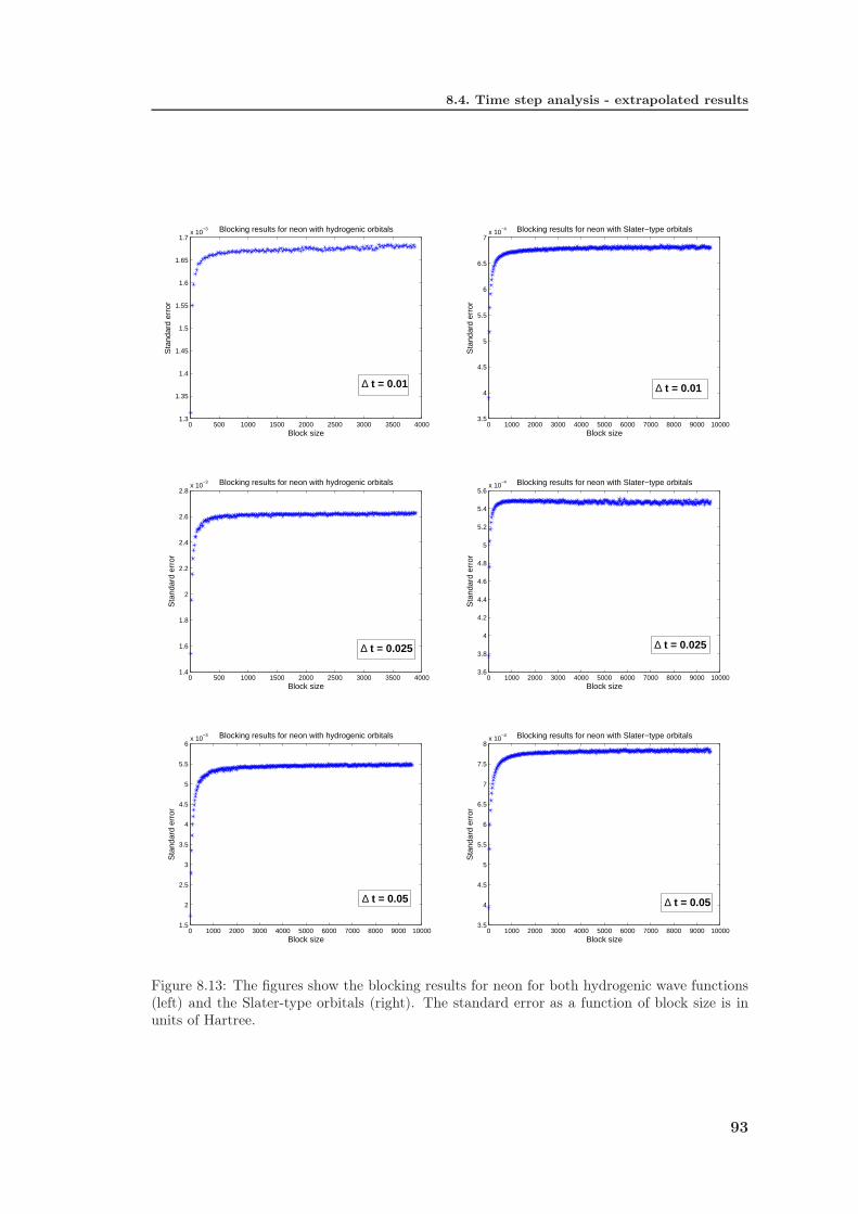
8.4. Time step analysis - extrapolated results
0 500 1000 1500 2000 2500 3000 3500 40001.3
1.35
1.4
1.45
1.5
1.55
1.6
1.65
1.7x 10
−3 Blocking results for neon with hydrogenic orbitals
Block size
Sta
ndar
d er
ror
∆ t = 0.01
0 1000 2000 3000 4000 5000 6000 7000 8000 9000 100003.5
4
4.5
5
5.5
6
6.5
7x 10
−4 Blocking results for neon with Slater−type orbitals
Block size
Sta
ndar
d er
ror
∆ t = 0.01
0 500 1000 1500 2000 2500 3000 3500 40001.4
1.6
1.8
2
2.2
2.4
2.6
2.8x 10
−3 Blocking results for neon with hydrogenic orbitals
Block size
Sta
ndar
d er
ror
∆ t = 0.025
0 1000 2000 3000 4000 5000 6000 7000 8000 9000 100003.6
3.8
4
4.2
4.4
4.6
4.8
5
5.2
5.4
5.6x 10
−4 Blocking results for neon with Slater−type orbitals
Block size
Sta
ndar
d er
ror
∆ t = 0.025
0 1000 2000 3000 4000 5000 6000 7000 8000 9000 100001.5
2
2.5
3
3.5
4
4.5
5
5.5
6x 10
−3 Blocking results for neon with hydrogenic orbitals
Block size
Sta
ndar
d er
ror
∆ t = 0.05
0 1000 2000 3000 4000 5000 6000 7000 8000 9000 100003.5
4
4.5
5
5.5
6
6.5
7
7.5
8x 10
−4 Blocking results for neon with Slater−type orbitals
Block size
Sta
ndar
d er
ror
∆ t = 0.05
Figure 8.13: The figures show the blocking results for neon for both hydrogenic wave functions(left) and the Slater-type orbitals (right). The standard error as a function of block size is inunits of Hartree.
93

Chapter 8. VMC Results
Magnesium with hydrogenic wave functions
∆t Energy Standard error
0.05 −199.85 2.1 · 10−2
0.25 −197.530 8.1 · 10−3
0.01 −196.818 3.8 · 10−3
Extrapolated −196.152 6.6 · 10−3
Table 8.10: The table shows the energies from the time step extrapolation, and standard errorsfrom the blocking method for magnesium with hydrogen-like wave functions.
Silicon with hydrogenic wave functions
∆t Energy Standard error
0.1 −298.00 5.9 · 10−2
0.05 −291.87 4.2 · 10−2
0.01 −284.352 6.7 · 10−3
Extrapolated −282.750 9.5 · 10−3
Table 8.11: The table shows the energies from the time step extrapolation, and standard errorsfrom the blocking method for silicon with hydrogen-like wave functions.
Helium with Slater-type orbitals
∆t Energy Standard error
0.1 −2.88876 2.3 · 10−5
0.05 −2.88833 3.1 · 10−5
0.01 −2.88783 6.8 · 10−5
Extrapolated −2.88782 5.0 · 10−5
Table 8.12: The table shows the energies from the time step extrapolation, and standard errorsfrom the blocking method for helium with Slater-type orbitals.
Beryllium with Slater-type orbitals
∆t Energy Standard error
0.1 −14.61260 5.3 · 10−5
0.05 −14.60941 6.0 · 10−5
0.01 −14.6088 1.2 · 10−4
Extrapolated −14.60725 9.5 · 10−5
Table 8.13: The table shows the energies from the time step extrapolation, and standard errorsfrom the blocking method for beryllium with Slater-type orbitals.
94

8.4. Time step analysis - extrapolated results
Neon with Slater-type orbitals
∆t Energy Standard error
0.05 −128.9343 7.8 · 10−4
0.025 −128.7021 5.5 · 10−4
0.01 −128.6164 6.4 · 10−4
Extrapolated −128.5187 7.7 · 10−4
Table 8.14: The table shows the energies from the time step extrapolation, and standard errorsfrom the blocking method for neon with Slater-type orbitals.
Magnesium with Slater-type orbitals
∆t Energy Standard error
0.05 −204.174 1.9 · 10−3
0.025 −204.482 1.7 · 10−3
0.01 −204.737 2.1 · 10−3
Extrapolated −204.852 2.3 · 10−3
Table 8.15: The table shows the energies from the time step extrapolation, and standard errorsfrom the blocking method for neon with Slater-type orbitals.
Silicon with Slater-type orbitals
∆t Energy Standard error
0.05 −294.180 2.6 · 10−3
0.025 −294.665 2.2 · 10−3
0.01 −295.131 2.4 · 10−3
Extrapolated −295.315 2.8 · 10−3
Table 8.16: The table shows the energies from the time step extrapolation, and standard errorsfrom the blocking method for silicon with Slater-type orbitals.
95

Chapter 8. VMC Results
8.5 Discussions
In this section we compare our VMC results for helium, beryllium and neon with theVMC results from table 2.4 in [3]. For magnesium and silicon we compare with theresults from table I in [4].
Table 8.17 lists the energy results compared to our reference energies. We see howfor our case the helium energy is best calculated with the hydrogenic wave functions,rather than with the Slater-type orbitals. It seems as though the hydrogenic orbitalsmodel the helium atom better than the Slater-type orbitals. But as we shall see forlarger systems with more correlation, the Slater-type orbitals gives us an advantage.
For beryllium, the Slater-type orbitals seem to model the correlation between theelectrons more correctly, and produce a more correct ground state energy estimationthan by using hydrogenic wave functions. It seems as though the Jastrow factor is goodfor modelling the correlations that the Hartree-Fock optimization of wave functions hasnot already taken care of.
If we are to compare with the energies from [4], we clearly see that the Slaterdeterminants with hydrogenic wave functions do not estimate the silicon energy in agood way. A good argument for this is the fact that we have chosen a Slater determinantas if the two outmost electrons were bound to a 3p-state with ml = +1, correspondingto the real solid harmonics being coordinate x. This is because our Slater determinantcode is restricted to describe atoms with an equal number of spin up electrons as spindown electrons. Since the Hamiltonian does not interact with spin or orbital momentum,we simply choose ml = +1, disregarding Hund’s rules (see [2]). As seen in section 3.1.3however, the two outermost electrons in silicon both have spin up and have a totalangular momentum of one. The electrons could be configured in different ways, e.g. onein a 3p-orbital with ml = +1 and one in 3p with ml = 0, both with spin up. Theelectrons could also be excited into 3d-orbitals etc. To accommodate for this, we wouldhave needed to implement linear combinations of Slater determinants and also includemore single particle wave functions. Because of this, we see that our wave functionprobably is too primitive for this matter.
A troubling aspect however, is the behavior of the the extrapolated energies formagnesium and silicon using a Slater determinant with the Slater-type orbitals obtainedby the Hartree-Fock calculations by Clementi and Roetti in [10]. Our VMC calculationsactually give too attractive energies compared to the calculations in [4]. But if we
Energy comparison
Atom Reference energy Extr. energy with HWF Extr. energy with STO
Helium −2.903726(4) −2.89040(3.9) −2.88722(5.0)
Beryllium −14.6664(3) −14.50220(1.8) −14.60725(9.5)
Neon −128.884(4) −127.284(2.5) −128.5187(7.7)
Magnesium −200.0002(5) −196.152(6.6) −204.852(2.3)
Silicon −289.1970(10) −282.750(9.5) −295.315(2.8)
Table 8.17: The table shows the energies from the time step extrapolation, and standard errorsfrom the blocking method for neon with Slater-type orbitals. Helium, beryllium and neonenergies are compared with VMC calculations from [3], while magnesium and silicon energieshave been compared with VMC results from [4]. Energies are in units of Hartree.
96

8.5. Discussions
consider the VMC calculations from [4] to be accurate, our results contradict with thevariational principle (see section 4.3). If this is the case, there must be something wrongwith the code that we have developed. However, we have seen in table 8.3 that our Slaterdeterminant reproduces the Roothaan-Hartree-Fock energies from [10] quite nicely. Wealso saw the same when calculating a non-interacting system using a Slater determinantwith hydrogenic orbitals, so we might be wrong to question the Slater determinant atthis point.
By running the code with only a Slater determinant with STO and no Jastrow factor,we reproduce the Hartree-Fock energies. These energies are already very close to theresults from [4], so we should not expect any significant improvement from an additionalcorrelation factor. However, the energies are somehow underestimated when includingthe Jastrow factor.
We cannot overlook the possibility that the Jastrow function we have chosenin this work (see 5.1.2) has not been implemented correctly, but this still seemssomewhat unlikely as it produces good improvements when working with hydrogenicwave functions. With that being said, we see a trend for the larger systems neon,magnesium and silicon when we include the Jastrow factor. The calculations then tendto produce less accurate results. For magnesium and silicon the energies are muchtoo low for our liking, while for neon the Jastrow factor hardly improves the Hartree-Fock energy. In these three cases, the pure Hartree-Fock (Slater-type orbitals) Slaterdeterminant without the Jastrow functions produces the best results.
97


Chapter 9
Conclusion
In this thesis we have performed Variational Monte Carlo calculations on the helium,beryllium, neon, magnesium and silicon atoms in order to estimate the ground stateenergy of the systems. We have developed a code in C++ that uses either hydrogen-likewave functions or Slater-type orbitals as single-particle wave functions. The Slater-typeorbitals have been optimized by a Hartree-Fock calculation in [10]. The code uses theMetropolis-Hastings algorithm (see e.g. [3]) with importance sampling.
We have seen that the code that we have developed produces very good results forhelium and beryllium in addition to sensible results for neon. For magnesium and siliconhowever, we have struggled to get good results. We clearly see that when introducingthe Jastrow factor in addition to Slater-type orbitals, the energies are underestimatedcompared to the VMC calculations from [4].
Despite the problems we have encountered when dealing with larger systems, westill see that the Variational Monte Carlo machinery we have developed is working. Byreviewing the results from the pure Slater determinant calculations (without any Jastrowfactor), we see that the results come out perfectly.
In order to improve this model we can examine more closely the Jastrow functionwe have used in this work to see whether or not there could be an error in theimplementation. Another approach would be to introduce other Jastrow factors in orderto model the correlation more correctly, such as the ones used in [4].
To improve calculations for silicon and other open-shell systems, we can alsoimplement the possibility of having linear combinations of Slater determinants. Wesee from the discussion in 8.5 that for these systems, the Slater determinant we haveimplemented might not be good enough to describe the physics.
When we get our full VMC machinery up and running, with correlations and all, thenext step would be to perform a Green’s function Monte Carlo calculation (see [3]). Inorder to perform Green’s function Monte Carlo (GFMC) calculation, the method needsa starting point for the energy. An optimized Variational Monte Carlo energy is a goodchoice for this. A GFMC calculation is in theory an exact method, and will result in usbeing able to determine an accurate ground state wave function. With this we can definethe quantum mechanical density, which can be used to construct a density functionalfor atoms using the adiabatic-connection method described in [21]. By starting with abinitio calculations, we can then hopefully improve the density functionals that are usedto model materials.


Appendix A
Roothaan-Hartree-Fock results
In this part I will present Clementi and Roetti’s results from their Roothaan-Hartree-Fock calculations for atoms helium, beryllium, neon, magnesium and silicon. The tables’applications are explained in section 5.5.
Helium
Helium consists of 2 electrons and a core of charge 2e and has the electron distribution(1s)2. Table A.1 shows the Roothaan-Hartree-Fock(RHF) solution for Helium. The
n,λ Exponent, ξ 1s exp.coeff.
1S 1.41714 0.768381S 2.37682 0.223561S 4.39628 0.040821S 6.52699 −0.009941S 7.94525 0.00230
Table A.1: The table shows the Roothan-Hartree-Fock results for Helium.
tabulated Roothaan-Hartree-Fock ground state energy for Helium given in [10] is
E = −2.8616799 Eh,
where Eh is the Hartree unit given in section 3.1.4.
Beryllium
Beryllium has 4 electrons with a nucleus charged 4e and has electrons distributed as(1s)2(2s)2. Table A.2 shows the RHF-solution for beryllium. In [10] the total groundstate energy is calculated as
E = −14.573021 Eh.
Neon
The ten Neon electrons are distributed as (1s)2(2s)2(2p)6. Table A.3 shows the RHF-solution. The Roothaan-Hartree-Fock energy is
E = −128.54705 Eh.
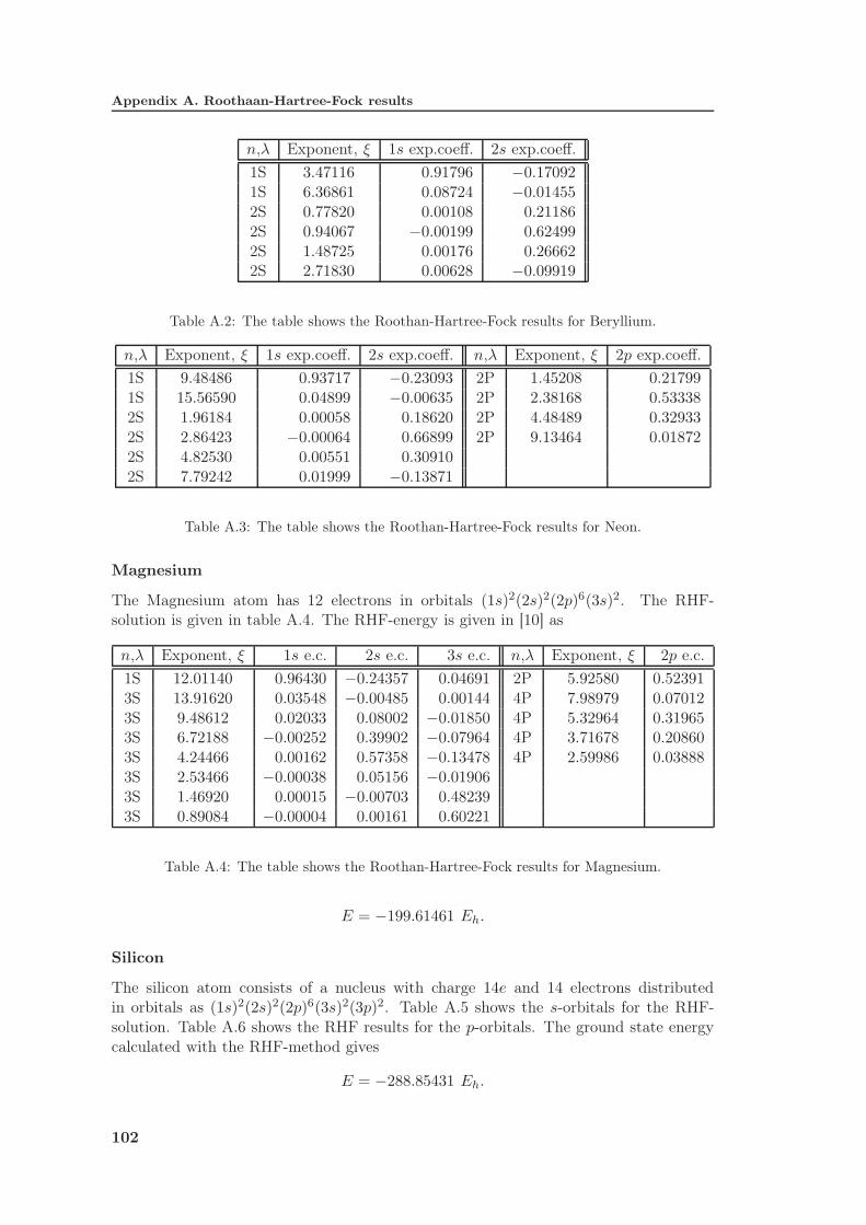
Appendix A. Roothaan-Hartree-Fock results
n,λ Exponent, ξ 1s exp.coeff. 2s exp.coeff.
1S 3.47116 0.91796 −0.170921S 6.36861 0.08724 −0.014552S 0.77820 0.00108 0.211862S 0.94067 −0.00199 0.624992S 1.48725 0.00176 0.266622S 2.71830 0.00628 −0.09919
Table A.2: The table shows the Roothan-Hartree-Fock results for Beryllium.
n,λ Exponent, ξ 1s exp.coeff. 2s exp.coeff. n,λ Exponent, ξ 2p exp.coeff.
1S 9.48486 0.93717 −0.23093 2P 1.45208 0.217991S 15.56590 0.04899 −0.00635 2P 2.38168 0.533382S 1.96184 0.00058 0.18620 2P 4.48489 0.329332S 2.86423 −0.00064 0.66899 2P 9.13464 0.018722S 4.82530 0.00551 0.309102S 7.79242 0.01999 −0.13871
Table A.3: The table shows the Roothan-Hartree-Fock results for Neon.
Magnesium
The Magnesium atom has 12 electrons in orbitals (1s)2(2s)2(2p)6(3s)2. The RHF-solution is given in table A.4. The RHF-energy is given in [10] as
n,λ Exponent, ξ 1s e.c. 2s e.c. 3s e.c. n,λ Exponent, ξ 2p e.c.
1S 12.01140 0.96430 −0.24357 0.04691 2P 5.92580 0.523913S 13.91620 0.03548 −0.00485 0.00144 4P 7.98979 0.070123S 9.48612 0.02033 0.08002 −0.01850 4P 5.32964 0.319653S 6.72188 −0.00252 0.39902 −0.07964 4P 3.71678 0.208603S 4.24466 0.00162 0.57358 −0.13478 4P 2.59986 0.038883S 2.53466 −0.00038 0.05156 −0.019063S 1.46920 0.00015 −0.00703 0.482393S 0.89084 −0.00004 0.00161 0.60221
Table A.4: The table shows the Roothan-Hartree-Fock results for Magnesium.
E = −199.61461 Eh.
Silicon
The silicon atom consists of a nucleus with charge 14e and 14 electrons distributedin orbitals as (1s)2(2s)2(2p)6(3s)2(3p)2. Table A.5 shows the s-orbitals for the RHF-solution. Table A.6 shows the RHF results for the p-orbitals. The ground state energycalculated with the RHF-method gives
E = −288.85431 Eh.
102

n,λ Exponent, ξ 1s exp.coeff. 2s exp.coeff. 3s exp.coeff.
1S 14.01420 0.96800 −0.25755 0.065953S 16.39320 0.03033 −0.00446 0.001853S 10.87950 0.02248 0.11153 −0.034613S 7.72709 −0.00617 0.40339 −0.103783S 5.16500 0.00326 0.55032 −0.192293S 2.97451 −0.00143 0.03381 −0.065613S 2.14316 0.00081 −0.00815 0.597323S 1.31306 −0.00016 0.00126 0.55390
Table A.5: The table shows the s-orbital Roothan-Hartree-Fock results for Silicon.
n,λ Exponent, ξ 2p exp.coeff. 3p exp.coeff.
2P 7.14360 0.54290 −0.115354P 16.25720 0.00234 −0.001894P 10.79720 0.04228 −004734P 6.89724 0.32155 −0.075524P 4.66598 0.22474 0.010414P 2.32046 0.00732 0.460754P 1.33470 −0.00105 0.576654P 0.79318 0.00041 0.06274
Table A.6: The table shows the p-orbital Roothan-Hartree-Fock results for Silicon.
103


Appendix B
Statistics
This appendix will give a short introduction to many key aspects regarding the statisticalterms used for calculating expectation values and its statistical error in the VariationalMonte Carlo process. We will follow the work in [22] quite closely in order to get all theimportant points across.
A probability distribution function(PDF), p(x), is a function that describes thefrequency of a stochastic value X to occur, that is
p(x) = Prob(X = x). (B.1)
This is for the discrete case.For the continuous case, p(x) represents a probability distribution, where we must
deal with probabilities of values being within some interval. That is, the probabilityof the stochastic variable X taking a value on the finite interval [a, b] is defined by anintegral
Prob(a ≤ X ≤ b) =
∫ b
ap(x)dx. (B.2)
All PDF’s must take values that are both positive and less or equal to unity, the absolutemaximum for any probability function to make sense. This means
0 ≤ p(x) ≤ 1, (B.3)
In addition to this, both the discrete and continuous PDF’s must be normalized to oneas
∑
i
p(xi) = 1, (B.4)
∫p(x)dx = 1. (B.5)
Moments and expectation values
Since our wave functions are continuous, our PDF will be so as well, and the expectationvalue of a function f(x) is given by
〈f〉 ≡ f(x)p(x)dx. (B.6)
We also have the moments, as special case of expectation values, where the n-th momentis
〈xn〉 ≡∫xnp(x)dx. (B.7)

Appendix B. Statistics
The mean, µ, is defined by the first moment, 〈x〉.The central moments are defined by
〈(x− 〈x〉)n〉 ≡∫
(x− 〈x〉)np(x)dx. (B.8)
The second central moment is called the variance, σ2X or Var(X), and can be written as
σ2X = Var(X) = 〈(x− 〈x〉)2〉
= 〈x2〉 − 〈x〉2. (B.9)
The standard deviation is then σ =√
〈x2〉 − 〈x〉2.
Correlated measurements
For now, we have been dealing with functions of one stochastic variable, so-calledunivariate PDF’s. However, a PDF may as well consist of many variables. These PDF’sare called multivariate PDF’s. The variables themselves are independent, or uncorrelated
is the multivariate PDF, P (x1, x2, ..., xn) can be factorized as
P (x1, x2, ..., xn) =
n∏
i=1
pi(xi), (B.10)
where pi(xi) are the univariate PDF’s.The so-called covariance of two stochastic variables, Xi and Xj , is defined as
Cov(Xi,Xj) ≡ 〈(xi − 〈xi〉)(xj − 〈xj〉)〉 = 〈xixj〉 − 〈xi〉〈xj〉. (B.11)
We see that for j = i this reduces to the variance of Xi, that is
Cov(Xi,Xi) = Var(Xi) = 〈x2i 〉 − 〈xi〉2. (B.12)
If the variables Xi and Xj are independent, or uncorrelated, the PDF’s will factorize asin Eq. (B.10), and we will have 〈xixj〉 = 〈xi〉〈xj〉. This will give Cov(Xi,Xj) = 0, wheni 6= j.
Consider linear combinations of stochastic variables Xi and Yj as
U =∑
i
aiXi, (B.13)
andV =
∑
j
bjYj, (B.14)
where ai and bj are scalar coefficients. As given in [23], we will have
Cov(U, V ) =∑
i,j
aibjCov(Xi, Yj). (B.15)
Since Var(Xi) = Cov(Xi,Xi), the variance of U will be
Var(U) =∑
i,j
aiajCov(Xi,Xj), (B.16)
106

which for uncorrelated variables will be reduced to
Var(U) =∑
i
a2iCov(Xi,Xi) =
∑
i
a2iVar(Xi), (B.17)
and
Var
(∑
i
aiXi)
)=∑
i
a2iVar(Xi). (B.18)
Approximations for finite data sets
Consider a computational experiment which produces a sequence of n stochastic values
x1, x2, . . . , xn, (B.19)
which we will call the n measurements of our sample. We can hereby define the sample
mean as
xn ≡ 1
n
n∑
k=1
xk, (B.20)
with the sample variance and sample covariance being
Var(x) ≡ 1
n
n∑
k=1
(xk − xn)2 (B.21)
and
Cov(x) ≡ 1
n
∑
kl
(xk − xn)(xl − xn), (B.22)
respectively. This sample covariance is a measure of the correlation between succeedingvalues in the sample. These values are not the same as the mean µX , Var(X) andCov(X) defined by the exact PDF, pX(x), but approximations to these quantities.
In the limit where n→ ∞ it can be shown that the sample mean, xn approaches thetrue mean µX , that is
limn→∞
xn = µX , (B.23)
and xn can be seen as an estimate of µX . But how good is this approximation? Inorder to find this we also need the error estimate of our measurement. We can viewthe sample means themselves as measurements in a collection of sample means (severalexperiments). To calculate the statistical error, we need the PDF of the sample means,pXn
(x). The exact error will be given by the standard deviation of the sample means,errX , also called sample error. However, we don’t know the exact PDF, so we can onlycalculate an estimate of errX .
The sample mean, xn, can be treated as a stochastic variable Xn, because xn is alinear combination of stochastic variables Xi with 1/n as common coefficients. Thismeans we can write
Xn =1
n
n∑
i=1
Xi. (B.24)
We will now have pX(x) as the probability distributions of the sample means Xn, butwe cannot get a closed form expression for this. However, the central limit theorem (see[23]) opens for an approximation of pX(x) as n→ ∞. It states that
limn→∞
pX(x) =
(n
2πV ar(X)
)1/2
e−
n(x−xn)2
2V ar(X) , (B.25)
107

Appendix B. Statistics
which means that the PDF will approach a Gaussian distribution. This Gaussiandistribution will have a mean and variance which equal to the true mean and variance,µX and σ2
X .The error is given by
err2X = Var(Xn) =1
n2
∑
ij
Cov(Xi,Xj). (B.26)
This exact error needs the true means µX in order to be calculated. We will not be ableto do this unless we have the exact PDF’s of the variables Xi. However, we only havethe measurements in a sample, and not the actual PDF.
Instead, we estimate the true means µX by the sample means
µXi= 〈xi〉 ≈
1
n
n∑
k=1
xk = 〈x〉. (B.27)
The estimate of the covariance will then be
Cov(Xi,Xj) = 〈(xi − 〈xi〉)(xj − 〈xj〉)〉 ≈ 〈(xi − x)(xj − x)〉
≈ 1
n
n∑
l
(1
n
n∑
k
(xk − xn)(xl − xn)
)
=1
n
1
n
∑
kl
(xk − xn)(xl − xn)
=1
nCov(x). (B.28)
The error estimate can be written using Eq. (B.28) as
err2X =1
n2
∑
ij
Cov(Xi,Xj)
≈ 1
n2
∑
ij
1
nCov(x) =
1
n2n2 1
nCov(x)
=1
nCov(x). (B.29)
The same approximation goes for the variance, as
Var(Xi) = = 〈(xi − 〈xi〉)2〉 ≈ 〈(xi − x)2〉
=1
n
n∑
k=1
(xk − xn)2
= Var(x), (B.30)
which for uncorrelated stochastic variables will give an error estimation as
err2X =1
n2
∑
ij
Cov(Xi,Xj)
=1
n2
∑
i
Var(Xi) ≈1
n2
∑
i
Cov(x)
=1
nVar(x). (B.31)
108
Autocorrelation function and correlation time
As given in [22], we can rewrite the error as
err2X =1
nCov(x) =
1
nVar(x) +
1
n(Cov(x) − Var(x))
=1
n2
n∑
k=1
(xk − xn)2 +
2
n2
∑
k<l
(xk − xn)(xl − xn). (B.32)
We see the first term is just the variance, so the second term must be the error correctionwhen the variables are correlated. By now introducing partial sums on the form
fd =1
n
n−d∑
k=1
(xk − xn)(xk+d − xn), (B.33)
we can write the correlation term as
2
n2
∑
k<l
(xk − xn)(xl − xn) =2
n
n−1∑
d=1
fd, (B.34)
where now fd is a measure of how correlated values separated by a distance d are. Bydividing fd by Var(x), we can define the autocorrelation function:
κd =fd
Var(x). (B.35)
We see that fd equals the sample variance, Var(x), when d = 0, so the autocorrelationfunction has a value of 1 for d = 0.
We can now rewrite the sample error as
err2X =1
nVar(x) +
2
nVar(x)
n−1∑
d=1
fdVar(x)
=
(1 + 2
n−1∑
d=1
κd
)1
nVar(x)
=τ
nVar(x), (B.36)
where τ ,
τ = 1 + 2
n−1∑
d=1
κd, (B.37)
is called the autocorrelation time and can be used to define the effective number ofmeasurements, neff = n/τ , for us to simply approximate the error by the samplevariance.
109


Appendix C
DFP and energy minimization
Since we wish to minimize the energy using our Variational Monte Carlo machinery, animportant part is to find the optimal parameters for the wave function. That is, theparameters for the wave function which minimizes the energy.
A rather brute force first approach is to manually vary the parameters and plotthe results as in section 8.2. This will give a good estimate of what the optimalparameters are, but will in general not be precise enough for more quantitatively precisemeasurements.
The method we use is a so-called quasi-Newton method, the Davidon-Fletcher-
Powell-algorithm (DFP) as given in [12]. This method builds on the conjugate gradientmethod (CGM) and the steepest descent method (both are described in [12]). Thesetechniques however, are respectively too costly numerically, or too brute force for ourliking.
Both CGM and DPF are based on approximating a function of variational parame-ters, f(x), by a quadratic form, where now x is the set of i variational parameters. Thisis done by writing the Taylor series of f(x) at some point P, as
f(x) = f(P) +∑
i
∂f
∂xi+
1
2
∂2f
∂xi∂xj. . .
≈ c− b · x +1
2x · A · x (C.1)
where now
c ≡ f(P) b ≡ −∇f |P [A]ij ≡∂2f
∂xi∂xj
∣∣∣P
. (C.2)
The matrix A is called the Hessian matrix, the matrix containing all second derivatives.The gradient can easily be calculated as
∇f = A · x− b. (C.3)
In the DFP method, we don’t have to calculate the exact Hessian, A, which takes a lotof computation time. The goal is then to iteratively construct a sequence of matrices,Hi, such that
limi→∞
Hi = A−1. (C.4)
By its name, it should be clear that the Newton method for finding the zero of thegradient of function is similar to the quasi-Newton method. For the Newton method,

Appendix C. DFP and energy minimization
we have to second order, near a current iteration point xi, the following
f(x) = f(xi) + (x − xi) · ∇f(xi) +1
2(x − xi) ·A · (x − xi) (C.5)
and∇f(x) = ∇f(xi) + A · (x − xi). (C.6)
In order to find the next iteration point using Newton’s method, we use that ∇f(x) = 0,giving
x − xi = −A−1 · ∇f(xi). (C.7)
The quasi-Newton method is introduced since we do not compute the exact Hessian andits inverse, but an approximation H ≈ A−1. As explained in [12], this approach canoften be better than using the true Hessian, as the matrix H is constructed in such away that it is always positive-definite and symmetric. The true Hessian is generally notalways positive-definite when we are far from the minimum, which can lead to movingtowards increasing values of f instead of decreasing values.
If we subtract Eq. (C.7) at xi+1 from the same equation at xi, we get
xi+1 − xi = A−1 · (∇fi+1) −∇fi)), (C.8)
where now fj = f(xj). At the point xi+1 we also have that Hi+1 is a good approximationfor A−1, yielding
xi+1 − xi = Hi+1 · (∇fi+1) −∇fi)). (C.9)
The “outer” product of two vectors, u and v, is given as, u ⊗ v. As opposed to the“inner” product of two vectors
u · v = uTv (C.10)
which returns a scalar, the “outer” product,
u⊗ v = uvT , (C.11)
returns a matrix. Component (u ⊗ v)ij is simply given as (u⊗ v)ij = uivj .The DPF updating formula for Hi+1 is given in [12] as
Hi = Hi+1 +(xi+1 − xi) ⊗ (xi+1 − xi)
(xi+1 − xi) · (∇fi+1 −∇fi)
− [Hi · (∇fi+1 −∇fi)] ⊗ [Hi · (∇fi+1 −∇fi)](∇fi+1 −∇fi) · Hi · (∇fi+1 −∇fi)
. (C.12)
We have used the function dfpmin.c from [12] which uses this quasi-Newton methodfor finding a minimum for f(x), while finding an approximation for the inverse Hessian.This method takes as input a function that returns the mean energy, and a functionthat calculates the gradient of the energy.
In this thesis we have a function f = E, the mean of the local energy operator, EL, asgiven in 4.4.1. To use the DFP method we must have the gradient of f , that is the firstderivatives of the energy expectation value with respect to the variational parameters,xi. The first derivatives of the energy expectation value are given in [14] as
∂E
∂xi= Ei =
⟨ψiψEL +
Hψiψ
− 2Eψiψ
⟩
= 2
⟨ψiψ
(EL − E)
⟩= 2
⟨ψiψEL
⟩− 2
⟨ψiψ
⟩E (C.13)
112

where ψi = ∂ψ/∂xi. The expectation values in Eq. (C.13) cannot be calculated easilyusing closed form expressions, and must be evaluated numerically. In this work we havejust used the simple three-point estimation of the first derivative
f ′(x) ≈ f(x+ h) − f(x− h)
2h, (C.14)
with h = 0.001.
113


Bibliography
[1] J. J. Brehm and W. J. Mullin, Introduction to the Structure of Matter (Wiley, 1989).
[2] D. Griffiths, Introduction to Quantum Mechanics - International Edition (PearsonEducation International, 2005).
[3] B. Hammond, W. Lester, and P. Reynolds, Monte Carlo Methods in Ab Initio
Quantum Chemistry (World Scientific, 1994).
[4] M. Casula and S. Sorella, Journal of Chemical Physics 119, 6500 (2003).
[5] B. Stroustrup, The C++ Programming Language (Addison-Wesley Longman Pub-lishing Co., Inc., 2000).
[6] T. Helgaker, P. Jørgensen, and J. Olsen, Molecular Electronic-Structure Theory
(Wiley, 2000).
[7] M. L. Boas, Mathematical Methods in the Physical Sciences (Wiley International,2006).
[8] S. Raimes, Many-Electron Theory (North-Holland Pub. Co., 1972).
[9] M. Hjorth-Jensen, Computational Physics (2010).
[10] E. Clementi and C. Roetti, Atomic Data and Nuclear Data Tables 14, 177 (1974).
[11] I. Shavitt and R. J. Bartlett, Many-Body Methods in Chemistry and Physics
(Cambridge University Press, 2009).
[12] W. H. Press, S. A. Teukolsky, W. T. Vetterling, and B. P. Flannery, Numerical
Recipes: The Art of Scientific Computing (Cambridge University Press, 2007).
[13] M. E. Newman and G. E. Barkema, Monte Carlo Methods in Statistical Phyiscs
(Oxford University Press, 1999).
[14] C. J. Umrigar and C. Filippi, Physical Review Letters 94, 150201 (2005).
[15] J. M. Thijssen, Computational Physics (Cambridge, 2007).
[16] J. Moskowitz and M. Kalos, International Journal of Quantum Chemistry 20, 1107(1981).
[17] W. Krauth, Statistical Mechanics: Algorithms and Computations (Oxford Univer-sity Press, 2006).
[18] H. Flyvbjerg and H. G. Petersen, Journal of Chemical Physics 91, 461 (1989).

[19] A. Sarsa, J. Boronat, and J. Casulleras, Journal of Chemical Physics 116, 5956(2002).
[20] C. Barbieri, D. V. Neck, and M. Degroote, ArXiv e-print: arXiv:1004.2607 (2010).
[21] A. M. Teale, S. Coriani, and T. Helgaker, Journal of Chemical Physics 130, 104111(2009).
[22] M. Røstad, Efficient Quantum Monte Carlo Calculations of Many-Body Systems
(University of Oslo, 2004).
[23] J. Rice, Mathematical Statistics and Data Analysis (Duxbury, 1995).