variations in embodied energy and carbon emission intensities of construction materials

Environmental Impact Assessment Review 49 (2014) 31–48

Contents lists available at ScienceDirect

Environmental Impact Assessment Review

j ourna l homepage: www.e lsev ie r .com/ locate /e ia r

Variations in embodied energy and carbon emission intensities ofconstruction materials

Wan-Mohd-Sabki Wan Omar a,b, Jeung-Hwan Doh a,⁎, Kriengsak Panuwatwanich a

a Griffith School of Engineering, Griffith University, Gold Coast Campus, Queensland 4222, Australiab School of Environmental Engineering, Universiti Malaysia Perlis, 02600 Arau, Perlis, Malaysia

⁎ Corresponding author. Tel.: +61 7 5552 9141; fax: +E-mail address: [email protected] (J.-H. Doh).

http://dx.doi.org/10.1016/j.eiar.2014.06.0030195-9255/© 2014 Elsevier Inc. All rights reserved.

a b s t r a c t
a r t i c l e i n f o
Article history:Received 9 February 2014Received in revised form 20 June 2014Accepted 23 June 2014Available online xxxx

Keywords:VariationParameterEmbodied energyCarbon emissionAustraliaMalaysia

Identification of parameter variation allows us to conductmore detailed life cycle assessment (LCA) of energy andcarbon emission material over their lifecycle. Previous research studies have demonstrated that hybrid LCA(HLCA) can generally overcome the problems of incompleteness and accuracy of embodied energy (EE) and car-bon (EC) emission assessment. Unfortunately, the current interpretation and quantification procedure has notbeen extensively and empirically studied in a qualitative manner, especially in hybridising between the processLCA and I-O LCA. To determine this weakness, this study empirically demonstrates the changes in EE and EC in-tensities caused by variations to key parameters in material production. Using Australia and Malaysia as a casestudy, the results are compared with previous hybrid models to identify key parameters and issues. The param-eters considered in this study are technological changes, energy tariffs, primary energy factors, disaggregationconstant, emission factors, and material price fluctuation. It was found that changes in technological efficiency,energy tariffs and material prices caused significant variations in the model. Finally, the comparison of hybridmodels revealed that non-energy intensivematerials greatly influence the variations due to high indirect energyand carbon emission in upstreamboundary ofmaterial production, and as such, any decision related to thesema-terials should be considered carefully.

© 2014 Elsevier Inc. All rights reserved.

Introduction

Overview of hybrid life cycle assessment

Life cycle assessment (LCA) is used to quantify environmentalimpact for a product's entire life cycle, including raw material extrac-tion, material or product manufacturing, construction, operation andmaintenance, and demolition. This can be classified as either a top-down or bottom-up approach. The traditional LCA or process LCA,known as bottom-up approach, is considered most accurate in embod-ied energy and carbon assessment. However, it fails to include theupstream boundary of material production. The embodied energy andcarbon embodied in upstream boundary are those inputs used furtherupstream in supplying goods and services to the main life cycle stages(Crawford, 2004). There are four steps to conduct hybrid LCA: (1) derivean I-O LCA model; (2) extract the most important pathway for theevaluated sector (e.g. plastic products and structural metal productssector); (3) derive specific data for the evaluated sector or components;and (4) substitute the case-specific LCA data into the I-Omodel (Treloaret al., 2000).

61 7 5552 8065.

More than 90% of energy and carbon emissions emanate from theupstream boundary of the supply chain in product manufacturing(Nässén et al., 2007). Due to the complexity of upstream inventoryanalysis in terms of time and labour consumption, the traditional LCAoften uses processed data available within commercial databases suchas Ecoinvent, GaBi, SimaPro, Athena and etc. Contrary to the processLCA, the top-down approach based on Input–Output (I-O) data (I-OLCA) includes a wider system boundary of the entire economic supplychain. However, I-O LCA inherits uncertainty, data aggregation, homo-geneity assumption, age of data and capital equipment (Crawford,2004).

Recently, the hybrid LCA has been developed as an effective methodfor assessing EE and EC emissions for the whole supply chain ofmaterials or products while maintaining the accuracy of process data(Acquaye, 2010; Crawford, 2004; Lee and Ma, 2013; Suh and Huppes,2005; Treloar, 1998; Wan Omar et al., 2012). The hybrid LCA can be de-fined as a combination of physical andmonetary units or the integrationof a process and I-O data. The flow of materials in process LCA and I-OLCA are expressed in physical (e.g. MJ, GJ, MJ/kg, and GJ/m2) andmonetary quantities (e.g. RM$, RM$/RM$, MJ/RM$, and GJ/RM$)(Acquaye, 2010). The I-O LCA provides a top-down linear microeco-nomic approach to explain the industrial structure in which the sectoralmonetary transaction data are used in an inter-industry model to

http://crossmark.crossref.org/dialog/?doi=10.1016/j.eiar.2014.06.003&domain=pdf

http://dx.doi.org/10.1016/j.eiar.2014.06.003

mailto:[email protected]

http://dx.doi.org/10.1016/j.eiar.2014.06.003

http://www.sciencedirect.com/science/journal/01959255

32 W.-M.-S. Wan Omar et al. / Environmental Impact Assessment Review 49 (2014) 31–48

account the complex interdependencies of industries (Lenzen et al.,2003).

Although, the hybrid LCA is widely used to overcome the limitationsof process approach, it still depends on the I-O data, which consists ofhighly aggregated industry sectors such as building construction thatcan cause variations to the hybrid LCA inventory (Dixit et al., 2013).Variations to energy and carbon emissions over the life cycle of buildingmaterials are known as uncertainties. These are due to stochastic varia-tion and a lack of knowledge of precise parameter values (Gustavssonand Sathre, 2006). Generally, hybrid LCA has five types of uncertainty:data inventory, system cut-off error, sector or product aggregation,and temporal and geographic uncertainty (Williams et al., 2009). Datauncertainty occurs in input due to inadequate parameters and data.Cut-off and truncation errors in the hybrid LCA can lead to a high levelof uncertainty in inventory data (Lee andMa, 2013). Cut-off error occurswhen the definition of system boundary is inconsistent whereas trunca-tion occurs between process and I-O inventory. Previous studies havebeen proposed to improve hybrid models by reducing uncertainty be-tween process and I-O data, but further improvement is also neededwhen integrating process and I-O data.

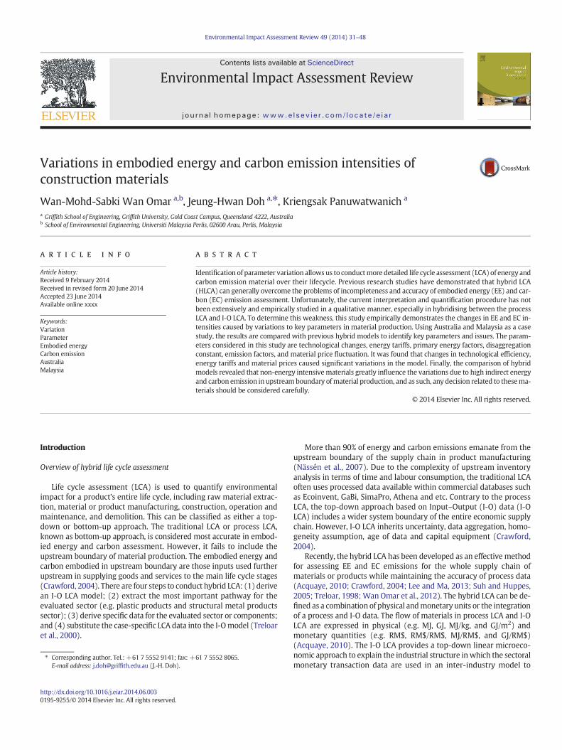
The iterative nature of hybrid LCA means more detailed assessmentneeds to be conducted to attain more reliable data. Previous studiesproposed methodologies to identify uncertainty and variability in lifecycle inventory (LCI) analysis (Heijungs, 1996; Huijbregts et al., 2003;Williams et al., 2009). For example, Heijungs (1996) outlined operation-al and generic methods for identifying key issues for further analysis indetailed LCI. Key issues were defined as the areas where product orprocess improvement leads to highest environmental improvement,as depicted in Fig. 1. Small changes that have large consequences(hot-spots) are crucial to the subsequent details of LCI, and are furtheridentified as (Heijungs, 1996):

• Areas that represent highly sensitive parameters where small changeshave great impact and must be accurately known prior to drawingconclusions; and

• Areas that represent highly sensitive parameters whereas smallchanges have great impact and might be affected by alternativeproduct or process design.

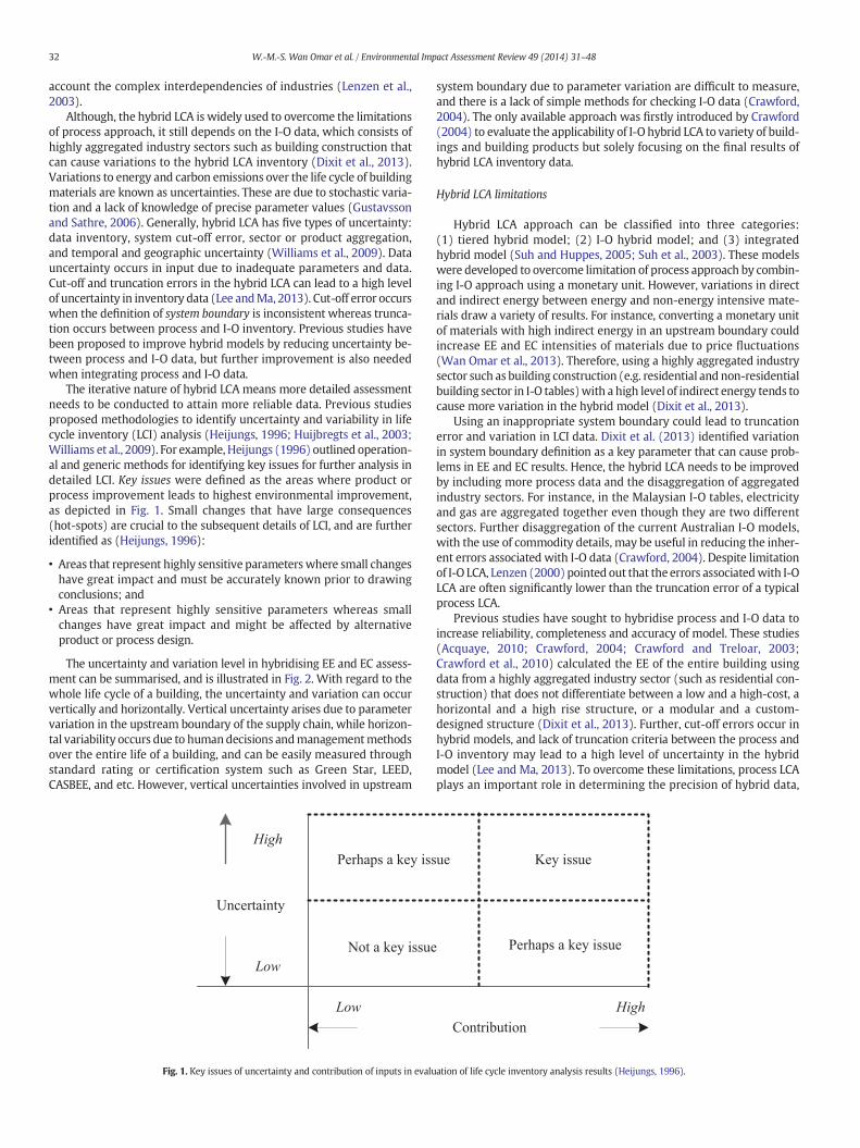
The uncertainty and variation level in hybridising EE and EC assess-ment can be summarised, and is illustrated in Fig. 2. With regard to thewhole life cycle of a building, the uncertainty and variation can occurvertically and horizontally. Vertical uncertainty arises due to parametervariation in the upstream boundary of the supply chain, while horizon-tal variability occurs due to humandecisions andmanagementmethodsover the entire life of a building, and can be easily measured throughstandard rating or certification system such as Green Star, LEED,CASBEE, and etc. However, vertical uncertainties involved in upstream

High

Low

Uncertainty

Low

Not a key issue

Perhaps a key iss

Fig. 1. Key issues of uncertainty and contribution of inputs in evalu

system boundary due to parameter variation are difficult to measure,and there is a lack of simple methods for checking I-O data (Crawford,2004). The only available approach was firstly introduced by Crawford(2004) to evaluate the applicability of I-O hybrid LCA to variety of build-ings and building products but solely focusing on the final results ofhybrid LCA inventory data.

Hybrid LCA limitations

Hybrid LCA approach can be classified into three categories:(1) tiered hybrid model; (2) I-O hybrid model; and (3) integratedhybrid model (Suh and Huppes, 2005; Suh et al., 2003). These modelswere developed to overcome limitation of process approach by combin-ing I-O approach using a monetary unit. However, variations in directand indirect energy between energy and non-energy intensive mate-rials draw a variety of results. For instance, converting a monetary unitof materials with high indirect energy in an upstream boundary couldincrease EE and EC intensities of materials due to price fluctuations(Wan Omar et al., 2013). Therefore, using a highly aggregated industrysector such as building construction (e.g. residential and non-residentialbuilding sector in I-O tables)with a high level of indirect energy tends tocause more variation in the hybrid model (Dixit et al., 2013).

Using an inappropriate system boundary could lead to truncationerror and variation in LCI data. Dixit et al. (2013) identified variationin system boundary definition as a key parameter that can cause prob-lems in EE and EC results. Hence, the hybrid LCA needs to be improvedby including more process data and the disaggregation of aggregatedindustry sectors. For instance, in the Malaysian I-O tables, electricityand gas are aggregated together even though they are two differentsectors. Further disaggregation of the current Australian I-O models,with the use of commodity details, may be useful in reducing the inher-ent errors associated with I-O data (Crawford, 2004). Despite limitationof I-O LCA, Lenzen (2000) pointed out that the errors associatedwith I-OLCA are often significantly lower than the truncation error of a typicalprocess LCA.

Previous studies have sought to hybridise process and I-O data toincrease reliability, completeness and accuracy of model. These studies(Acquaye, 2010; Crawford, 2004; Crawford and Treloar, 2003;Crawford et al., 2010) calculated the EE of the entire building usingdata from a highly aggregated industry sector (such as residential con-struction) that does not differentiate between a low and a high-cost, ahorizontal and a high rise structure, or a modular and a custom-designed structure (Dixit et al., 2013). Further, cut-off errors occur inhybrid models, and lack of truncation criteria between the process andI-O inventory may lead to a high level of uncertainty in the hybridmodel (Lee and Ma, 2013). To overcome these limitations, process LCAplays an important role in determining the precision of hybrid data,

Contribution

High

Perhaps a key issue

ue Key issue

ation of life cycle inventory analysis results (Heijungs, 1996).

Construction OperationRepair &

maintenanceDisposal

Variability due to assumptions

Manufacturing of

construction material

& components

Raw material

extraction or

recycled materials

I-O

inventory

Hybri

d L

CA

Pro

cess

LC

A

Unce

rtai

nty

due

to

par

amet

er v

aria

tion

Construction

Erection and installation

Waste

Transportation

Heating & cooling

Ventilation

Lighting

Reuse

Recycle

Disposal

Replacement

Horizontal

variability

Ver

tica

l

unce

rtai

nty

Fig. 2. Uncertainty and variation level in hybridising EE and EC assessment.

33W.-M.-S. Wan Omar et al. / Environmental Impact Assessment Review 49 (2014) 31–48

and theproportion of the I-O inventorywould be lower than for thepro-cess LCA (Lee and Ma, 2013).

Research objectives

Previous research studies demonstrated the changes of EE and ECintensities of materials and products over a certain period of time. Thechanges of EE and EC could be influenced by one or combination of thefollowing factors: system boundaries, method of EE analysis, geographiclocation, primary and delivered energy, age of data sources, sources ofdata, completeness of data, and temporal representativeness (Dixitet al., 2010). However, these factors have not been empirically studiedto identify their relative contributions to the EE and EC intensities.

Currently, there is limited research conducted to empirically investi-gate the impact of parameter variations in EE and EC intensities, particu-larly to study how this parameter can be incorporated into EE and ECanalysis and to what extent this parameter influences the variations ofEE and EE intensities. Therefore, the purpose of this paper is to identifyfactors and issues that have a strong influence on hybridmodels resultingfrom material production, and to determine the different effects of pa-rameters variation on hybrid model. Subsequently, comparisons weremade between previous studies to determine key significant variationunderwhich circumstances hybridmodel have higher than other and fur-ther proposed methodology to reduce variation in hybrid LCA model.

To overcome hybrid LCA limitations, this paper demonstrates hybridLCA at material production levels first, then computing the EE and EC ofthe entire building or its components using actual quantity of materials,energy and construction equipment (process data). This model is moreflexible, consistent, and capable of reducing uncertainty and variation inthe hybrid model. As such, this approach would assist in generating EEand EC estimates specific to building design and types of building inagreement with, and providing contextual support to, previous studies(Dixit et al., 2013).

In order to achieve the above objectives, the paper is organised asfollows. In Methodology and assumption section, the methodology andassumption are firstly discussed in detail. Further, the detaileddescriptions of parameters in hybrid LCA model are presented inDescriptions of parameter variations section and variations in eachparameter are evaluated. The variations of each parameter are then incor-porated in hybrid LCAmodel and results and discussions on EE and EC in-tensities of materials and products are presented in Results and

discussions section. Subsequently, the results from hybrid LCA modelare compared with previous research based on Australian, New Zealandand Malaysian I-O tables and presented in Comparison with previousstudies section. Finally, this paper draws conclusions, identifies limita-tions and proposes future researches in Discussion and conclusionsection.

Methodology and assumption

Deriving indirect EE and EC emission intensities for reference cases

Using I-O tables provided by the Australian Bureau of Statistic (ABS)and Malaysian Department of Statistics (DOS) enables the determinationof uncertainty and variation due to geographical conditions. I-O tableswere publicly published with a lag time of up to 5 years. Malaysian I-Otables were published every five years (latest Malaysian 2005 I-O tableswere published in 2010), whereas Australians I-O tables were updatedevery two to three years (latest Australian 2007 I-O tables werepublished in 2011). Therefore, 2005 I-O tables were chosen as referencecases for comparison between Australia and Malaysia. Indirect EE andEC intensities of reference materials were based on the 2005 I-O tableswhich were publicly available in Australia and Malaysia respectively.

There are different aggregations apply to the energy supply sectorsshown in the Australian and Malaysian I-O tables. For example, in theAustralian I-O tables, data are available at division, subdivision, groupand class levels, with each product or commodity being allocated to anI-O product group (Australian Bureau of Statistics, 2006). Meanwhile,the Malaysian I-O tables are classified according to division, group, classand item (Malaysian Department of Statistics, 2000). Energy tariffs, pri-mary energy factors, disaggregation constants and emission factorswere derived to convert monetary units in the supply chain into physicalunits that were then combined with process data (Acquaye and Duffy,2010; Wan Omar et al., 2014).

Deriving hybrid EE and EC emission intensities for reference cases

Hybridising EE and EC requires attention to two issues— namely theallocation of interface between process LCA and I-O LCA, and the poten-tial for double counting (Alvarez-Gaitan et al., 2013). Importantly, thehybrid LCA needs to be improved by including more process data and


disaggregation of the industry sector (Dixit et al., 2013; Lee and Ma,2013).

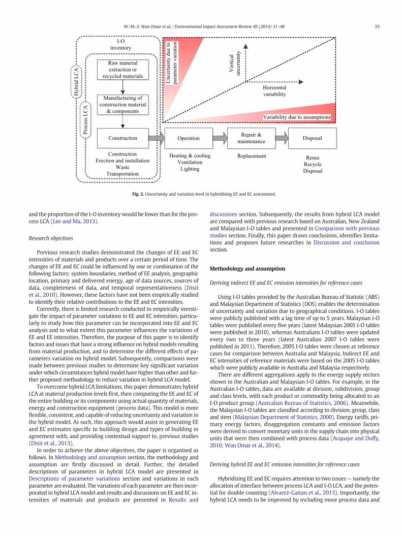
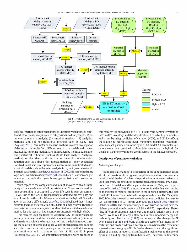
Hybrid LCA incorporates process data into I-O analysis during calcu-lation of the hybrid energy intensity as show in Fig. 3. Crawford (2005)explained that in calculating a building's hybrid embodied energy andcarbon intensities, the first step is to calculate the hybrid energy inten-sity of the most common basic materials. In this research, the hybridembodied energy and carbon intensities of the basicmaterialwas deter-mined by adding thedifference between the I-O total energy intensity ofsector n and input–output direct energy intensity of the pathrepresenting the basic material to the process energy intensity of thematerial. This I-O difference represents the energy intensity of the ma-terial unaccounted for by the process analysis as a result of truncation(or setting the system boundary). The embodied energy and carbon in-tensities of materials, as estimated using hybrid model (Crawford,2005), are given in Eqs. (1) and (2) below:

EIm ¼ EID þ TEI−DEIð Þ � Cm½ � ð1Þ

ECO2‐eIm ¼ ECO2‐eID þ TCO2‐eI−DCO2‐eIð Þ � Cm½ � ð2Þ

where, EIm is the energy intensity of a material using hybrid LCA(MJ/kg); EID is the direct energy of a material from process LCA(MJ/kg); TEI is the total energy intensity of a material from I-O LCA(MJ/$); DEI is the direct energy intensity of a material from I-O LCA(MJ/$); ECO2-eIm is the carbon intensity of a material using hybridLCA (kg CO2-e/kg); ECO2-eID is the direct carbon intensity of a materi-al from process LCA (kg CO2-e/kg); TCO2-eI is the total carbon inten-sity of a material from I-O LCA (kg CO2-e/$); DCO2-eI is the directcarbon intensity of a material from I-O LCA (kg CO2-e/$); and Cm isthe material price ($/kg).

The second stepwas to calculate the direct and total embodied ener-gy intensities of material or product sector using Eqs. (3) and (4) belowrespectively by adding disaggregation constant (Acquaye, 2010).

DEIn ¼XE

e¼1

DRC � CD � Te � PEF ð3Þ

TEIn ¼XE

e¼1

TRC � CD � Te � PEF ð4Þ

where, DRC is the direct requirement coefficient ($/$); TRC is the totalrequirement coefficient ($/$); CD is the disaggregation constant (dimen-sionless); Te is the average energy tariffs (GJ/$); and PEF the is primaryenergy factors (dimensionless).

To estimate direct and total carbon coefficient, national emission fac-tor was employed to convert direct and total energy intensities to directand total carbon intensities. Using disaggregation constant was essen-tial to ensure individual emission factor can be assigned to its particularenergy sector. Hence, the direct and total carbon intensities for a partic-ular sector or product derived from I-O LCA was rewritten respectivelyas shown in Eqs. (5) and (6) respectively.

DCO2‐eI ¼XE

eDRCe

� Ce � P:E:FeCe � Ie ð5Þ

TCO2‐eI ¼XE

eTRCe

� Ce � P:E:FeCe � Ie ð6Þ

where,DCO2-eI is the direct carbon intensity for a particular sector orproduct output (kg CO2-e/$); Ie is the emission intensity of energysupply sector, e (kg CO2-e/GJ); and TCO2-eI is the total carbon intensityfor a particular sector or product output (kg CO2-e/$).

In order to identify total EE and EC intensities of a product (e.g.ready-mix concrete, precast concrete pipe, etc.) using hybrid LCA, directenergy and carbon of the product were obtained from I-O LCA whenprocess LCA was unavailable. The direct energy and carbon intensitiesof the product were derived from I-O LCA and were then multipliedby theproduct price. The total EE and EC of theproductwere formulatedby summing all EE and EC intensities ofmaterialswith direct energy andcarbon of the product as given in Eqs. (7) and (8) below.

EET ¼XM

m¼1

EIm �We � Qmð Þ þ DEIpdt � Cpdt ð7Þ

ECO2‐e;T ¼XM

m¼1

ECO2‐eIm �W � Qmð ÞDCO2‐eIpdt � Cpdt ð8Þ

where, EET is the total EE of a product using hybrid LCA (MJ/kg);W isthe material wastage factor; Qm is the quantity of material in theproduct manufacturing (kg/unit); DEIpdt is the direct energy intensityof a product using I-O LCA (MJ/$); Cpdt is the total price of a product($/kg); ECO2-e,T is the total EC of a product using hybrid LCA (MJ/kg);and DCO2-eIpdt is the direct carbon intensity of a product using I-O LCA(kg CO2-e/$).

Evaluation methods

A variety of factors can affect the energy and carbon emission ofbuildingmaterials over its entire lifecycle. These factors can be classifiedinto uncertainty and variability (Gustavsson and Sathre, 2006). Uncer-tainty occurs due to stochastic variation or lack of knowledge of preciseparameter values, while variability is identified as human decisions andmanagement methods. Uncertainty in LCI is categorised into parameteruncertainty, model uncertainty, and scenario uncertainty.

Parameter uncertainty occurs due to incomplete knowledge of truevalues of data, and management error in input values (Acquaye,2010). Data uncertaintymay arise due to data inaccuracy, lack of specif-ic data, data gaps, and unrepresentative data (Huijbregts et al., 2001).This uncertainty can be dealt with using techniques such as analyticalpropagation methods, stochastic models, fuzzy logic, and neuralnetworks.

Model uncertainty arises due to unknown interactions betweenmodels. Simplification of aspects that cannot be modelled in EE and ECanalysis such as temporal and spatial characteristic lost by aggregation,non-linear instead of linearmodel, or derivation of characteristicmodel,were identified as factors affecting the uncertainty in a model. This canbe mitigated by re-sampling different model formulations (Huijbregtset al., 2003), or using a combination of I-O LCA and process LCA(Williams et al., 2009).

Scenario uncertainties arise due to choices relating to functional unit,system boundaries, weighting of factors and forecasting. Huijbregtset al. (2003) suggested scenario uncertainty could be quantified by re-sampling different decision scenarios. For example, results can be calcu-lated for both a data set with high emission values and one with lowemission values. This technique involves investigating what effects dif-ferent sets of data, models and choices have on results (Acquaye, 2010).For example, in an analysis of parameter variations in embodied energyand carbon analysis of a building, the effects of high and low processembodied carbon intensities of building materials on the results canbe measured.

A number of techniques were identified for dealingwith uncertaintyand variability in LCI. Uncertainty analysis can be conducted using twoapproaches— onebased on calculating extremevalues, the other on sta-tistical methods (Heijungs, 1996). The first approach identifies lowerand upper values of every parameter and combines them to determinethe lower and upper values of the area. The second approach uses a

I-O direct energy

intensity (GJ/RM$)

I-O total energy

intensity (GJ/RM$)

I-O indirect

energy intensity

(GJ/RM$)

I-O indirect carbon

emission intensity

(kg CO2-e/RM$)

I-O direct carbon

emission intensity

(kg CO2-e/RM$)

Process EE &

EC intensity

(MJ/kg)

(kg CO2-e/kg)

(ICE 2.0)

Multiply

Subtract

Add

Multiply

Multiply

Extract

Multiply

Multiply

EE & EC intensity

of const. material

or product

Add

Process EE &

EC intensity

(MJ/kg)

(kg CO2-e/kg)

(EPD)

Australian &

Malaysia energy

balance 2005-2008

(IEA)

Australian &

Malaysia I-O

tables 2005-2008

(ABS & DOE)

Energy tariff

GJ/RM$

Tech. coeff.

(RM$/RM$)

Primary

energy factor

Disagg.

constant

Material

properties

(kg/m2)

Emission factor

(kg CO2-e/GJ)

Building

material or

product prices

(RM$/unit)

I-O LCA

Legend:

Process LCA

Hybrid LCA

Material

properties

(kg/m3)

Material

properties

(kg/m)

Multiply

Action

Fig. 3. Flowchart for hybrid EE and EC inventory methodology.(adopted from Acquaye, A. et al., 2011).


statistical method to establishmargins of uncertainty (margins of confi-dents). Uncertainty analysis can be categorised into four groups: (1) pa-rameter or scenario analysis; (2) sampling methods; (3) analyticalmethods; and (4) non-traditional methods such as fuzzy logic(Acquaye, 2010). Parameter or scenario analysis involves investigationof the impact on results from different sets of data, models and choices.Meanwhile, sampling methods are undertaken by iterative calculationusing statistical techniques such as Monte Carlo analysis. Analyticalmethods, on the other hand, are based on an explicit mathematicalequation such as a first order approximation of Taylor expansion.Non-traditional statistical approaches involve more complicated math-ematical models such as Bayesian analysis, fuzzy logic, neural network,and non-parametric statistics. González et al. (2002) incorporated fuzzylogic into LCA, whereas Shipworth (2002) conducted Bayesian analysisto model the embodied greenhouse gas emission of constructionmaterials.

With regard to the complexity and lack of knowledge about uncer-tainty of data, evaluation of all uncertainty in LCI was considered tootime-consuming to be applied to every life cycle impact assessment(LCIA). Due to the lack of transparency of detailed process data andlack of simple methods for I-O model evaluation, the hybrid LCA evalu-ation in LCI was a difficult task. Crawford (2004) believed that it is nec-essary to focus on the evaluation of LCI data at a higher level. Therefore,parameter or scenario analysis was identified as a suitable evaluationmethod for this research into quantifying uncertainty in hybrid LCA.

This research used coefficient of variation (COV) to identify changesin every parameter and the calculation of extreme values (minimumand maximum values) to be incorporated into the hybrid model. Limit-ing the selection of lower and upper values of each parameter does notaffect the results as sensitivity analysis is concerned with determiningonly minimum and maximum possible of EE and EC impacts(Basbagill et al., 2013). Two important components were proposed in

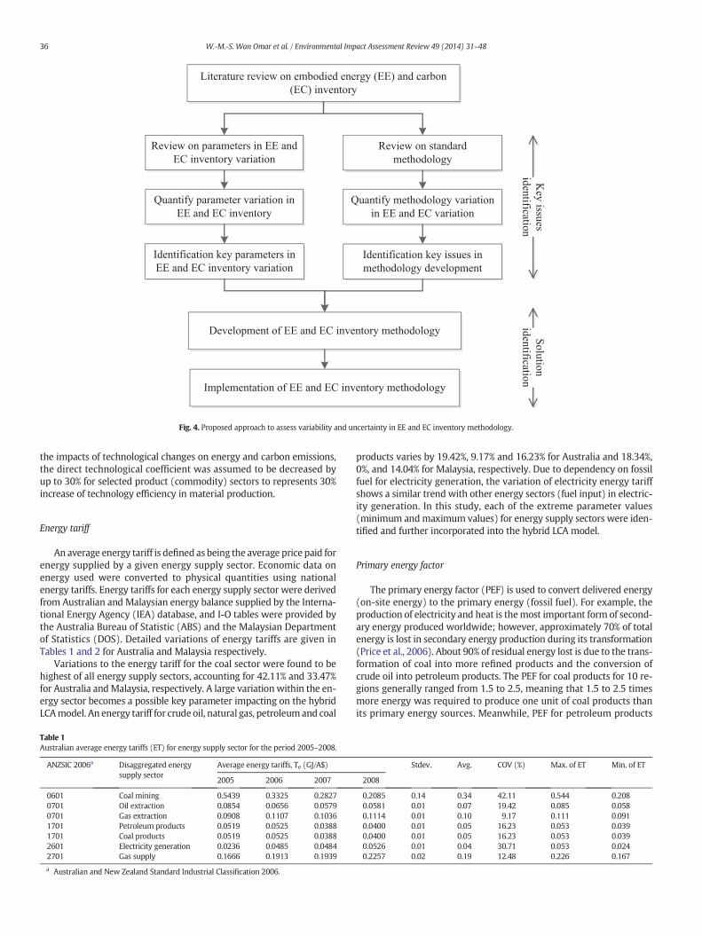
this research (as shown in Fig. 4): (1) quantifying parameter variationin EE and EC inventory, and the identification of possible key parametersand issues by using coefficient of variation (COV); and (2) identifyingthe solution by incorporating lower (minimum) and upper (maximum)values of each parameter into the hybrid LCAmodel. All parameter var-iations were then combined to identify impacts upon the hybrid LCA.Details of parameter variations are discussed in the following section.

Descriptions of parameter variations

Technological changes

Technological changes in production of building materials couldaffect the variation of energy consumption and carbon emission in ahybrid model. In the I-O tables, the production inducement effect wasused to identify the amount of domestic production changes by an addi-tional unit of final demand for a particular industry (Malaysian Depart-ment of Statistics, 2010). If an increase to a unit in the final demand ledto an increase of material production in the specified industry, this alsocould affect an increase in broader range of industries. The Malaysian2005 I-O tables showed an average inducement coefficient increase to0.61 as compared to 0.47 in the year 2000 (Malaysian Department ofStatistics, 2010). The manufacturing and construction sectors have thehighest production inducement of 2.88 and 0.75, respectively. There-fore, different production technology and types of energy used in theprocess could result in large differences to the embodied energy andcarbon figures. Baird et al. (1997) demonstrated the changes in EEover a period of time and found that three quarter of EE intensities ofmaterials and products drop an average of 41% whereas the remaindershowed a rise averaging 46%. He further demonstrated the significanteffect of changes in material manufacturing technology to the overallfigure of a building, ranging from 32% to 56%. Therefore, to determine

Literature review on embodied energy (EE) and carbon

(EC) inventory

Review on parameters in EE and

EC inventory variation

Review on standard

methodology

Quantify parameter variation in

EE and EC inventory

Quantify methodology variation

in EE and EC variation

Identification key parameters in

EE and EC inventory variation

Identification key issues in

methodology development

Development of EE and EC inventory methodology

Implementation of EE and EC inventory methodology

Key

issues

iden

tification

Solu

tion

iden

tification

Fig. 4. Proposed approach to assess variability and uncertainty in EE and EC inventory methodology.


the impacts of technological changes on energy and carbon emissions,the direct technological coefficient was assumed to be decreased byup to 30% for selected product (commodity) sectors to represents 30%increase of technology efficiency in material production.

Energy tariff

An average energy tariff is defined as being the average price paid forenergy supplied by a given energy supply sector. Economic data onenergy used were converted to physical quantities using nationalenergy tariffs. Energy tariffs for each energy supply sector were derivedfrom Australian and Malaysian energy balance supplied by the Interna-tional Energy Agency (IEA) database, and I-O tables were provided bythe Australia Bureau of Statistic (ABS) and the Malaysian Departmentof Statistics (DOS). Detailed variations of energy tariffs are given inTables 1 and 2 for Australia and Malaysia respectively.

Variations to the energy tariff for the coal sector were found to behighest of all energy supply sectors, accounting for 42.11% and 33.47%for Australia andMalaysia, respectively. A large variationwithin the en-ergy sector becomes a possible key parameter impacting on the hybridLCAmodel. An energy tariff for crude oil, natural gas, petroleumand coal

Table 1Australian average energy tariffs (ET) for energy supply sector for the period 2005–2008.

ANZSIC 2006a Disaggregated energysupply sector

Average energy tariffs, Te (GJ/A$)

2005 2006 2007

0601 Coal mining 0.5439 0.3325 0.28270701 Oil extraction 0.0854 0.0656 0.05790701 Gas extraction 0.0908 0.1107 0.10361701 Petroleum products 0.0519 0.0525 0.03881701 Coal products 0.0519 0.0525 0.03882601 Electricity generation 0.0236 0.0485 0.04842701 Gas supply 0.1666 0.1913 0.1939

a Australian and New Zealand Standard Industrial Classification 2006.

products varies by 19.42%, 9.17% and 16.23% for Australia and 18.34%,0%, and 14.04% for Malaysia, respectively. Due to dependency on fossilfuel for electricity generation, the variation of electricity energy tariffshows a similar trend with other energy sectors (fuel input) in electric-ity generation. In this study, each of the extreme parameter values(minimum andmaximum values) for energy supply sectors were iden-tified and further incorporated into the hybrid LCA model.

Primary energy factor

The primary energy factor (PEF) is used to convert delivered energy(on-site energy) to the primary energy (fossil fuel). For example, theproduction of electricity and heat is themost important form of second-ary energy produced worldwide; however, approximately 70% of totalenergy is lost in secondary energy production during its transformation(Price et al., 2006). About 90% of residual energy lost is due to the trans-formation of coal into more refined products and the conversion ofcrude oil into petroleum products. The PEF for coal products for 10 re-gions generally ranged from 1.5 to 2.5, meaning that 1.5 to 2.5 timesmore energy was required to produce one unit of coal products thanits primary energy sources. Meanwhile, PEF for petroleum products

Stdev. Avg. COV (%) Max. of ET Min. of ET

2008

0.2085 0.14 0.34 42.11 0.544 0.2080.0581 0.01 0.07 19.42 0.085 0.0580.1114 0.01 0.10 9.17 0.111 0.0910.0400 0.01 0.05 16.23 0.053 0.0390.0400 0.01 0.05 16.23 0.053 0.0390.0526 0.01 0.04 30.71 0.053 0.0240.2257 0.02 0.19 12.48 0.226 0.167

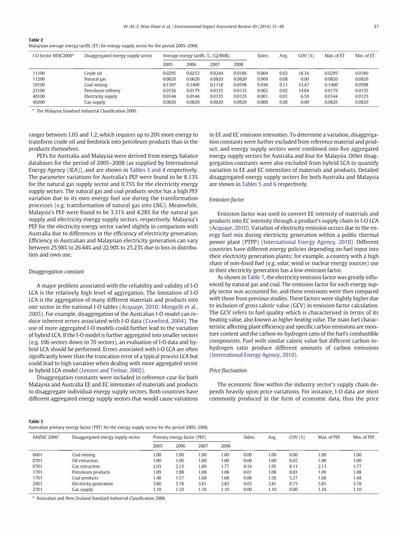
Table 2Malaysian average energy tariffs (ET) for energy supply sector for the period 2005–2008.

I-O Sector MSIC2000a Disaggregated energy supply sector Average energy tariffs, Te (GJ/RM$) Stdev. Avg. COV (%) Max. of ET Min. of ET

2005 2006 2007 2008

11100 Crude oil 0.0295 0.0253 0.0244 0.0186 0.004 0.02 18.34 0.0295 0.018611200 Natural gas 0.0820 0.0820 0.0820 0.0820 0.000 0.08 0.00 0.0820 0.082010100 Coal mining 0.1397 0.1400 0.1118 0.0598 0.038 0.11 33.47 0.1400 0.059823100 Petroleum refinery 0.0156 0.0179 0.0135 0.0135 0.002 0.02 14.04 0.0179 0.013540100 Electricity supply 0.0144 0.0144 0.0135 0.0125 0.001 0.01 6.59 0.0144 0.012540200 Gas supply 0.0820 0.0820 0.0820 0.0820 0.000 0.08 0.00 0.0820 0.0820

a The Malaysia Standard Industrial Classification 2000.


ranges between 1.05 and 1.2, which requires up to 20% more energy totransform crude oil and feedstock into petroleum products than in theproducts themselves.

PEFs for Australia and Malaysia were derived from energy balancedatabases for the period of 2005–2008 (as supplied by InternationalEnergy Agency (IEA)), and are shown in Tables 3 and 4 respectively.The parameter variations for Australia's PEF were found to be 8.13%for the natural gas supply sector and 0.75% for the electricity energysupply sectors. The natural gas and coal products sector has a high PEFvariation due to its own energy fuel use during the transformationprocesses (e.g. transformation of natural gas into LNG). Meanwhile,Malaysia's PEF were found to be 3.31% and 4.28% for the natural gassupply and electricity energy supply sectors, respectively. Malaysia'sPEF for the electricity energy sector varied slightly in comparison withAustralia due to differences in the efficiency of electricity generation.Efficiency in Australian and Malaysian electricity generation can varybetween 25.98% to 26.44% and 22.90% to 25.23% due to loss in distribu-tion and own use.

Disaggregation constant

A major problem associated with the reliability and validity of I-OLCA is the relatively high level of aggregation. The limitation of I-OLCA is the aggregation of many different materials and products intoone sector in the national I-O tables (Acquaye, 2010; Mongelli et al.,2005). For example, disaggregation of the Australian I-O model can re-duce inherent errors associated with I-O data (Crawford, 2004). Theuse of more aggregated I-O models could further lead to the variationof hybrid LCA. If the I-Omodel is further aggregated into smaller sectors(e.g. 106 sectors down to 70 sectors), an evaluation of I-O data and hy-brid LCA should be performed. Errors associated with I-O LCA are oftensignificantly lower than the truncation error of a typical process LCA butcould lead to high variation when dealing with more aggregated sectorin hybrid LCA model (Lenzen and Treloar, 2002).

Disaggregation constants were included in reference case for bothMalaysia and Australia EE and EC intensities of materials and productsto disaggregate individual energy supply sectors. Both countries havedifferent aggregated energy supply sectors that would cause variations

Table 3Australian primary energy factor (PEF) for the energy supply sector for the period 2005–2008.

ANZSIC 2006a Disaggregated energy supply sector Primary energy factor (PEF)

2005 2006 2007

0601 Coal mining 1.00 1.00 1.000701 Oil extraction 1.00 1.00 1.000701 Gas extraction 2.03 2.13 1.891701 Petroleum products 1.09 1.08 1.081701 Coal products 1.48 1.57 1.602601 Electricity generation 3.80 3.78 3.812701 Gas supply 1.10 1.10 1.10

a Australian and New Zealand Standard Industrial Classification 2006.

in EE and EC emission intensities. To determine a variation, disaggrega-tion constants were further excluded from referencematerial and prod-uct, and energy supply sectors were combined into five aggregatedenergy supply sectors for Australia and four for Malaysia. Other disag-gregation constants were also excluded from hybrid LCA to quantifyvariation in EE and EC intensities of materials and products. Detaileddisaggregated energy supply sectors for both Australia and Malaysiaare shown in Tables 5 and 6 respectively.

Emission factor

Emission factor was used to convert EE intensity of materials andproducts into EC intensity through a product's supply chain in I-O LCA(Acquaye, 2010). Variation of electricity emission occurs due to the en-ergy fuel mix during electricity generation within a public thermalpower plant (PTPP) (International Energy Agency, 2010). Differentcountries have different energy policies depending on fuel input intotheir electricity generation plants; for example, a country with a highshare of non-fossil fuel (e.g. solar, wind or nuclear energy sources) usein their electricity generation has a low emission factor.

As shown in Table 7, the electricity emission factorwas greatly influ-enced by natural gas and coal. The emission factor for each energy sup-ply sector was accounted for, and these emissions were then comparedwith those fromprevious studies. These factors were slightly higher dueto inclusion of gross caloric value (GCV) in emission factor calculation.The GCV refers to fuel quality which is characterised in terms of itsheating value, also known as higher heating value. Themain fuel charac-teristic affecting plant efficiency and specific carbon emissions aremois-ture content and the carbon-to-hydrogen ratio of the fuel's combustiblecomponents. Fuel with similar caloric value but different carbon-to-hydrogen ratio produce different amounts of carbon emissions(International Energy Agency, 2010).

Price fluctuation

The economic flow within the industry sector's supply chain de-pends heavily upon price variations. For instance, I-O data are mostcommonly produced in the form of economic data, thus the price

Stdev. Avg. COV (%) Max. of PEF Min. of PEF

2008

1.00 0.00 1.00 0.00 1.00 1.001.00 0.00 1.00 0.02 1.00 1.001.77 0.16 1.95 8.13 2.13 1.771.08 0.01 1.08 0.65 1.09 1.081.68 0.08 1.58 5.27 1.68 1.483.85 0.03 3.81 0.75 3.85 3.781.10 0.00 1.10 0.00 1.10 1.10

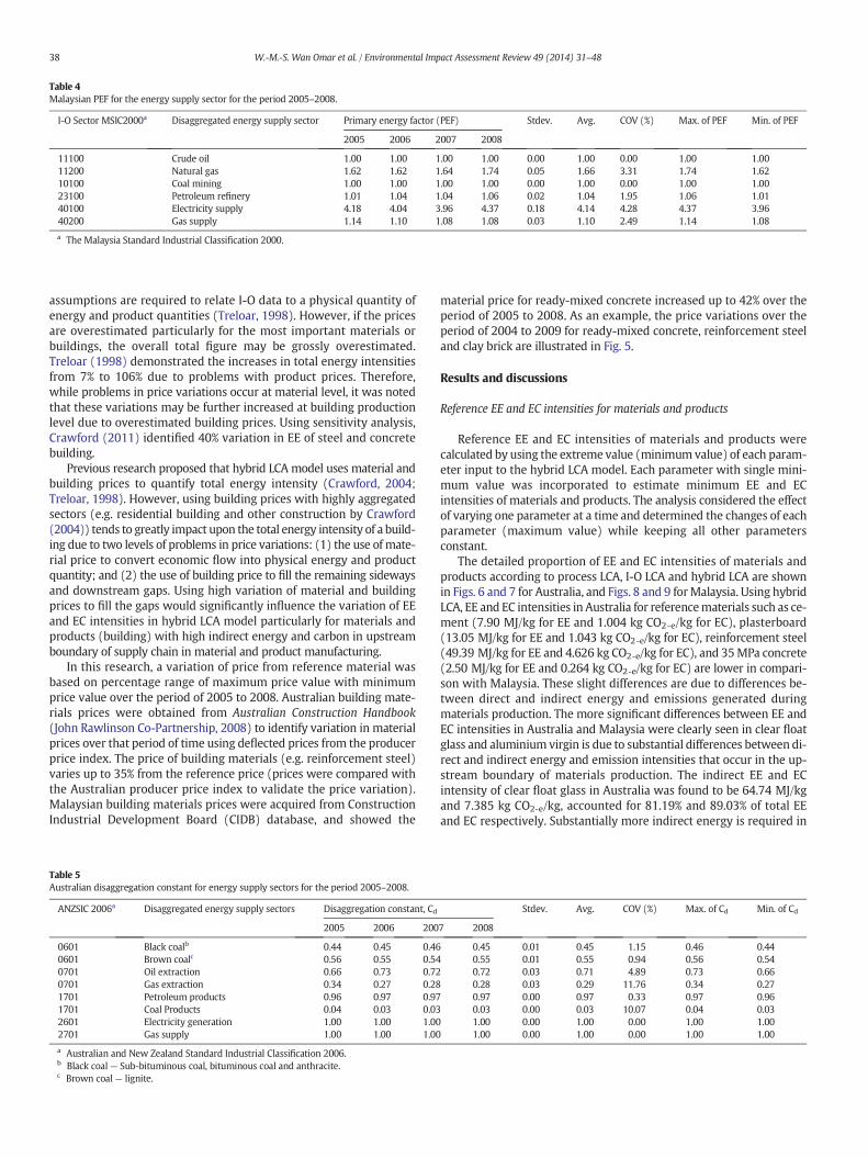
Table 4Malaysian PEF for the energy supply sector for the period 2005–2008.

I-O Sector MSIC2000a Disaggregated energy supply sector Primary energy factor (PEF) Stdev. Avg. COV (%) Max. of PEF Min. of PEF

2005 2006 2007 2008




assumptions are required to relate I-O data to a physical quantity ofenergy and product quantities (Treloar, 1998). However, if the pricesare overestimated particularly for the most important materials orbuildings, the overall total figure may be grossly overestimated.Treloar (1998) demonstrated the increases in total energy intensitiesfrom 7% to 106% due to problems with product prices. Therefore,while problems in price variations occur at material level, it was notedthat these variations may be further increased at building productionlevel due to overestimated building prices. Using sensitivity analysis,Crawford (2011) identified 40% variation in EE of steel and concretebuilding.

Previous research proposed that hybrid LCA model uses material andbuilding prices to quantify total energy intensity (Crawford, 2004;Treloar, 1998). However, using building prices with highly aggregatedsectors (e.g. residential building and other construction by Crawford(2004)) tends to greatly impact upon the total energy intensity of a build-ing due to two levels of problems in price variations: (1) the use of mate-rial price to convert economic flow into physical energy and productquantity; and (2) the use of building price to fill the remaining sidewaysand downstream gaps. Using high variation of material and buildingprices to fill the gaps would significantly influence the variation of EEand EC intensities in hybrid LCA model particularly for materials andproducts (building) with high indirect energy and carbon in upstreamboundary of supply chain in material and product manufacturing.

In this research, a variation of price from reference material wasbased on percentage range of maximum price value with minimumprice value over the period of 2005 to 2008. Australian building mate-rials prices were obtained from Australian Construction Handbook(John Rawlinson Co-Partnership, 2008) to identify variation in materialprices over that period of time using deflected prices from the producerprice index. The price of building materials (e.g. reinforcement steel)varies up to 35% from the reference price (prices were compared withthe Australian producer price index to validate the price variation).Malaysian building materials prices were acquired from ConstructionIndustrial Development Board (CIDB) database, and showed the

Table 5Australian disaggregation constant for energy supply sectors for the period 2005–2008.

ANZSIC 2006a Disaggregated energy supply sectors Disaggregation constant, Cd

2005 2006 200

0601 Black coalb 0.44 0.45 0.460601 Brown coalc 0.56 0.55 0.540701 Oil extraction 0.66 0.73 0.720701 Gas extraction 0.34 0.27 0.281701 Petroleum products 0.96 0.97 0.971701 Coal Products 0.04 0.03 0.032601 Electricity generation 1.00 1.00 1.002701 Gas supply 1.00 1.00 1.00

a Australian and New Zealand Standard Industrial Classification 2006.b Black coal— Sub-bituminous coal, bituminous coal and anthracite.c Brown coal— lignite.

material price for ready-mixed concrete increased up to 42% over theperiod of 2005 to 2008. As an example, the price variations over theperiod of 2004 to 2009 for ready-mixed concrete, reinforcement steeland clay brick are illustrated in Fig. 5.

Results and discussions

Reference EE and EC intensities for materials and products

Reference EE and EC intensities of materials and products werecalculated by using the extreme value (minimum value) of each param-eter input to the hybrid LCA model. Each parameter with single mini-mum value was incorporated to estimate minimum EE and ECintensities of materials and products. The analysis considered the effectof varying one parameter at a time and determined the changes of eachparameter (maximum value) while keeping all other parametersconstant.

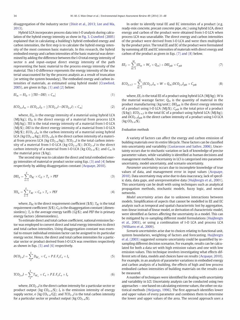
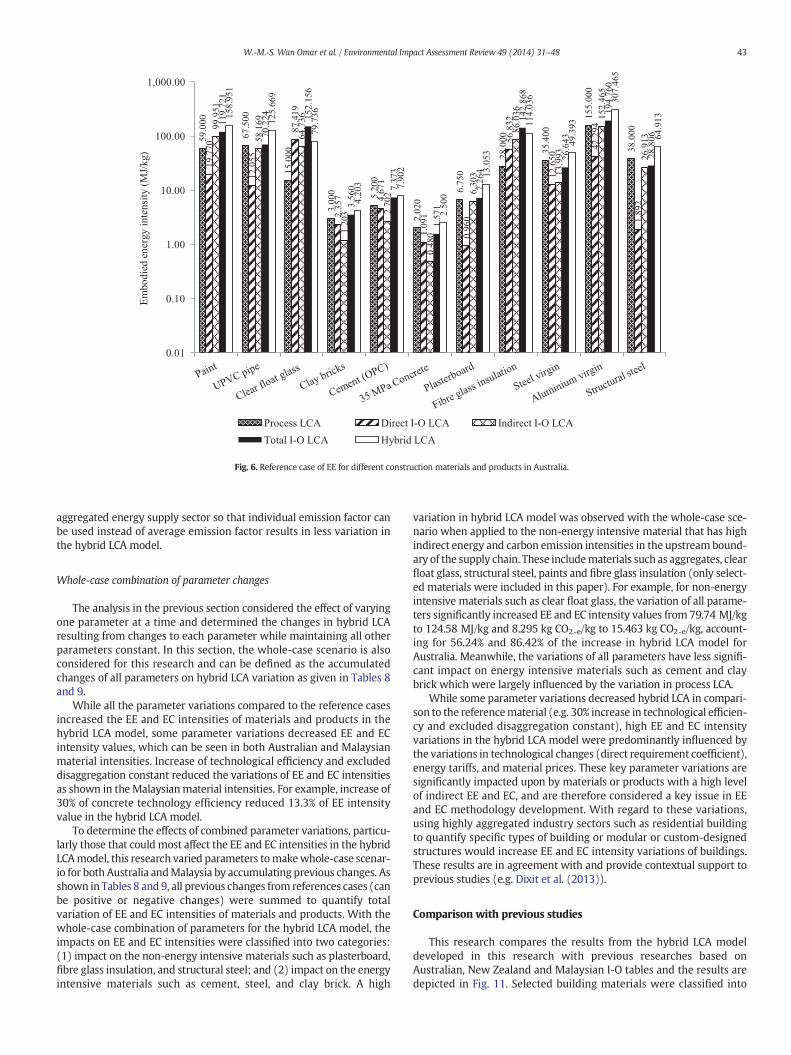
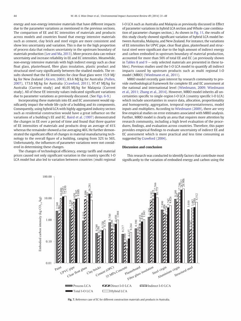
The detailed proportion of EE and EC intensities of materials andproducts according to process LCA, I-O LCA and hybrid LCA are shownin Figs. 6 and 7 for Australia, and Figs. 8 and 9 forMalaysia. Using hybridLCA, EE and EC intensities in Australia for referencematerials such as ce-ment (7.90 MJ/kg for EE and 1.004 kg CO2-e/kg for EC), plasterboard(13.05 MJ/kg for EE and 1.043 kg CO2-e/kg for EC), reinforcement steel(49.39 MJ/kg for EE and 4.626 kg CO2-e/kg for EC), and 35MPa concrete(2.50 MJ/kg for EE and 0.264 kg CO2-e/kg for EC) are lower in compari-son with Malaysia. These slight differences are due to differences be-tween direct and indirect energy and emissions generated duringmaterials production. The more significant differences between EE andEC intensities in Australia and Malaysia were clearly seen in clear floatglass and aluminium virgin is due to substantial differences between di-rect and indirect energy and emission intensities that occur in the up-stream boundary of materials production. The indirect EE and ECintensity of clear float glass in Australia was found to be 64.74 MJ/kgand 7.385 kg CO2-e/kg, accounted for 81.19% and 89.03% of total EEand EC respectively. Substantially more indirect energy is required in

Stdev. Avg. COV (%) Max. of Cd Min. of Cd

7 2008

0.45 0.01 0.45 1.15 0.46 0.440.55 0.01 0.55 0.94 0.56 0.540.72 0.03 0.71 4.89 0.73 0.660.28 0.03 0.29 11.76 0.34 0.270.97 0.00 0.97 0.33 0.97 0.960.03 0.00 0.03 10.07 0.04 0.031.00 0.00 1.00 0.00 1.00 1.001.00 0.00 1.00 0.00 1.00 1.00

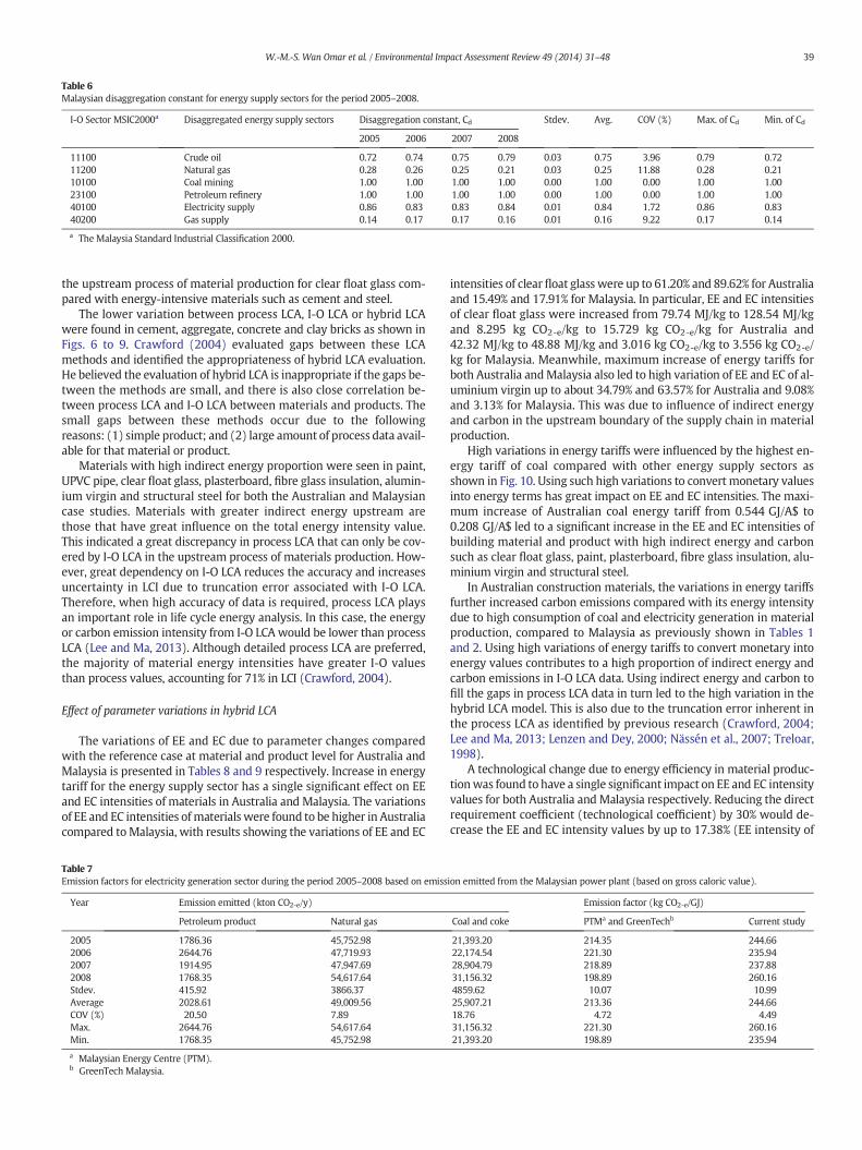
Table 6Malaysian disaggregation constant for energy supply sectors for the period 2005–2008.

I-O Sector MSIC2000a Disaggregated energy supply sectors Disaggregation constant, Cd Stdev. Avg. COV (%) Max. of Cd Min. of Cd

2005 2006 2007 2008




the upstream process of material production for clear float glass com-pared with energy-intensive materials such as cement and steel.

The lower variation between process LCA, I-O LCA or hybrid LCAwere found in cement, aggregate, concrete and clay bricks as shown inFigs. 6 to 9. Crawford (2004) evaluated gaps between these LCAmethods and identified the appropriateness of hybrid LCA evaluation.He believed the evaluation of hybrid LCA is inappropriate if the gaps be-tween the methods are small, and there is also close correlation be-tween process LCA and I-O LCA between materials and products. Thesmall gaps between these methods occur due to the followingreasons: (1) simple product; and (2) large amount of process data avail-able for that material or product.

Materials with high indirect energy proportion were seen in paint,UPVC pipe, clear float glass, plasterboard, fibre glass insulation, alumin-ium virgin and structural steel for both the Australian and Malaysiancase studies. Materials with greater indirect energy upstream arethose that have great influence on the total energy intensity value.This indicated a great discrepancy in process LCA that can only be cov-ered by I-O LCA in the upstream process of materials production. How-ever, great dependency on I-O LCA reduces the accuracy and increasesuncertainty in LCI due to truncation error associated with I-O LCA.Therefore, when high accuracy of data is required, process LCA playsan important role in life cycle energy analysis. In this case, the energyor carbon emission intensity from I-O LCA would be lower than processLCA (Lee and Ma, 2013). Although detailed process LCA are preferred,the majority of material energy intensities have greater I-O valuesthan process values, accounting for 71% in LCI (Crawford, 2004).

Effect of parameter variations in hybrid LCA

The variations of EE and EC due to parameter changes comparedwith the reference case at material and product level for Australia andMalaysia is presented in Tables 8 and 9 respectively. Increase in energytariff for the energy supply sector has a single significant effect on EEand EC intensities of materials in Australia and Malaysia. The variationsof EE and EC intensities ofmaterials were found to be higher in Australiacompared toMalaysia, with results showing the variations of EE and EC

Table 7Emission factors for electricity generation sector during the period 2005–2008 based on emiss

Year Emission emitted (kton CO2-e/y)

Petroleum product Natural gas

2005 1786.36 45,752.982006 2644.76 47,719.932007 1914.95 47,947.692008 1768.35 54,617.64Stdev. 415.92 3866.37Average 2028.61 49,009.56COV (%) 20.50 7.89Max. 2644.76 54,617.64Min. 1768.35 45,752.98

a Malaysian Energy Centre (PTM).b GreenTech Malaysia.

intensities of clearfloat glass were up to 61.20% and 89.62% for Australiaand 15.49% and 17.91% for Malaysia. In particular, EE and EC intensitiesof clear float glass were increased from 79.74 MJ/kg to 128.54 MJ/kgand 8.295 kg CO2-e/kg to 15.729 kg CO2-e/kg for Australia and42.32 MJ/kg to 48.88 MJ/kg and 3.016 kg CO2-e/kg to 3.556 kg CO2-e/kg for Malaysia. Meanwhile, maximum increase of energy tariffs forboth Australia andMalaysia also led to high variation of EE and EC of al-uminium virgin up to about 34.79% and 63.57% for Australia and 9.08%and 3.13% for Malaysia. This was due to influence of indirect energyand carbon in the upstream boundary of the supply chain in materialproduction.

High variations in energy tariffs were influenced by the highest en-ergy tariff of coal compared with other energy supply sectors asshown in Fig. 10. Using such high variations to convert monetary valuesinto energy terms has great impact on EE and EC intensities. The maxi-mum increase of Australian coal energy tariff from 0.544 GJ/A$ to0.208 GJ/A$ led to a significant increase in the EE and EC intensities ofbuilding material and product with high indirect energy and carbonsuch as clear float glass, paint, plasterboard, fibre glass insulation, alu-minium virgin and structural steel.

In Australian construction materials, the variations in energy tariffsfurther increased carbon emissions compared with its energy intensitydue to high consumption of coal and electricity generation in materialproduction, compared to Malaysia as previously shown in Tables 1and 2. Using high variations of energy tariffs to convert monetary intoenergy values contributes to a high proportion of indirect energy andcarbon emissions in I-O LCA data. Using indirect energy and carbon tofill the gaps in process LCA data in turn led to the high variation in thehybrid LCA model. This is also due to the truncation error inherent inthe process LCA as identified by previous research (Crawford, 2004;Lee and Ma, 2013; Lenzen and Dey, 2000; Nässén et al., 2007; Treloar,1998).

A technological change due to energy efficiency in material produc-tionwas found to have a single significant impact on EE and EC intensityvalues for both Australia and Malaysia respectively. Reducing the directrequirement coefficient (technological coefficient) by 30% would de-crease the EE and EC intensity values by up to 17.38% (EE intensity of

ion emitted from the Malaysian power plant (based on gross caloric value).

Emission factor (kg CO2-e/GJ)

Coal and coke PTMa and GreenTechb Current study

21,393.20 214.35 244.6622,174.54 221.30 235.9428,904.79 218.89 237.8831,156.32 198.89 260.164859.62 10.07 10.9925,907.21 213.36 244.6618.76 4.72 4.4931,156.32 221.30 260.1621,393.20 198.89 235.94

0

20

40

60

80

100

120

140

2003 2004 2005 2006 2007 2008 2009 2010

Pro

du

cer

pri

ce i

nd

ex

Year

Ready mixed concrete

Reinforcement steel

Clay brick

Fig. 5. Price variation in selected construction materials based on producer price index forthe period 2004–2009.


35MPa concrete) and 15.98% (EC intensity of clear float glass), and thiscould be further reduced if more renewable energy (e.g. solar, wind,geothermal, etc.) is used to replace fossil fuel. High indirect energyand carbon in EE and EC intensities in materials productions such aspaint, clearfloat glass, plasterboard andfibre glass insulationwould fur-ther impact upon variation in the hybrid LCA model (negative value)due to the substantial influence of energy and carbon in the upstreamboundary in material production. For instance, a 30% increase in energyefficiency of concrete (30% reduction in the direct energy requirementfor cement, aggregate and water) decreased the EE and EC intensitiesby 17.38% and 13.99% in Australia and 13.30% and 9.39% in Malaysia.

Aside from the influence of technological changes in materials andproducts manufacturing, the difference in EE and EC intensity valueswas also affected by the complexity of the economic structure and sys-tem. For example in manufacturing industry, Gutowski (2007) relatedenergy and carbon emission with the gross domestic product which isdepending on the technological change in the domestic production (In-termediate production). This was supported by Lenzen and Treloar(2002), who analysed the data from Börjesson and Gustavsson (2000)using energy intensity obtained from I-O data, based on the prices inAustralia. They concluded that the variation in energy intensity couldrely on differences in production structures between Australia andSweden and/or scope of the studies. Gustavsson and Sathre (2006)added that using I-O LCA (top-down economic technique) to comparethe physical impact of using different construction materials may beeffected by differences in overall economic structures. Nevertheless,derivation of I-O data for both Australia and Malaysia shows a similarinfluence from variations of energy tariffs and technological changes.While materials with high direct energy and carbon (e.g. cement, claybrick, and reinforcement steel) have less significant impact on thehybrid LCAmodel, the energy tariff and technological change variationsgreatly impact upon materials and products with high indirect energyand carbon (e.g. clear float glass, plasterboard, fibre glass insulation,and paint).

Further, Lenzen and Treloar (2002) demonstrated the majordiscrepancies between Australian and Swedish energy intensities thatexist for softwood, mineral wool insulation, plasterboard and plastic.These variations are due to the plasterboard and plastic products requir-ing more energy in their immediate manufacturing in Sweden, whilethe remaining items are more energy-intensive in Australia. They alsoagreed that these variations were due either to differences betweenthe Australian and Swedish production systems (e.g. input structure,economics of scale, etc.), or simply because of the complete differentof production layers between two countries.

A single variation in PEF for both Australia andMalaysia has less im-pact on EE and EC intensities of materials and products. A maximum

increase of PEF (particularly the natural gas and electricity supply sec-tors) has less a significant impact on the hybrid LCA model. Using max-imum PEF values between the periods of 2005 to 2008 showed the EEand EC intensities of materials values increase up to about 4.09% and2.76% (clear float glass) for Australia and 13.02% and 4.80% (plaster-board) for Malaysia respectively. In particularly, the EE and EC intensi-ties for clear float glass slightly increased from 79.74 MJ/kg to83.0 MJ/kg and 8.295 kg CO2-e/kg to 8.524 kg CO2-e/kg. Meanwhile, EEand EC intensities for plasterboard also slightly increased from19.16 MJ/kg to 21.66 MJ/kg and 1.503 kg CO2-e/kg to 1.576 kg CO2-e/kg. The influence of parameter variations on other energy intensivema-terials is less significant (e.g. cement, clay brick, steel virgin, etc.), com-pared to that on less energy intensivematerials such as clear float glass,plasterboard, or plastic product, which have a large proportion of indi-rect energy and carbon in upstream boundary of material production.Treloar (1998) derived PEF based on previous findings and furtherused by Pullen (2007) and Crawford (2004) to identify indirect energyand carbon intensities from I-O data. These PEF values were further in-cluded to identify hybrid LCA variations. Using these PEF values only in-creased EE and EC intensities ofmaterials by up to 1% to 2% in the hybridLCA model.

Using a disaggregation constant for aggregated energy supply sec-tors had less impact on the variation of EC intensities in the hybridLCAmodel. In general, disaggregation constants were used to enable in-dividual emission factors to be assigned to their energy supply sector inorder to convert energy requirements to carbon emission intensities.Without disaggregation constants, EE and EC intensity values for paintvaried up to 4.06% (4.06% of EE reduction) and less than 1% (less than1% of EC reduction) in Australia and 10.31% (10.31% of EE reduction)and 12.60% (12.60% of EC reduction) in Malaysia respectively. Asshown in Tables 8 and 9, overall EE and EC intensities of materials inthe hybrid LCAmodel slightly decreased from the reference case.Mean-while, the variations of EE and EC intensities in Malaysia were highercompared with Australia due to aggregated energy supply sectors inMalaysian I-O tables such as electricity and gas supply (e.g. aggregatedinto electricity and gas supply as shown in Malaysian 2005 I-O tables).Therefore, with high energy consumption and carbon emission factorsfor electricity generation, using this disaggregated energy supply sectorincreased the variations of EE and EC intensities in hybrid LCA model.Acquaye (2010) also demonstrated the variation of EC intensity up to2.6 times when disaggregation constants are used to disaggregate ener-gy and non-energy supply sector such as disaggregation of coal, peat,and crude oil (energy supply sector) from metal ore extraction sector(non-energy supply sector). On the other hand, EC intensities areoverestimated more than 2.6 times compared to when disaggregationare employed.

Similar impact of parameter variations can be found on other EE andEC intensities of materials with high indirect energy and carbon in theupstream boundary of material production, but were excluded fromthis paper. Therefore, materials with high indirect energy and carbonhave the largest influence on the hybrid LCA model. Using aggregatedindustry sectors such as residential construction itself with high indirectenergy and carbon in upstream boundary of building system to quantifythe embodied energy and carbon of an entire buildingmay also result ina significant variation of EE and EC intensities of a building (building isconsidered as a product). Using sensitivity analysis for energy data un-certainty, Crawford (2011) identified 40% variation of EE for steel andconcrete building using hybrid LCA. On the other hand, this variationarises due to the aggregated building sector used and price fluctuationof building in the hybrid LCA model.

An increasedmaterial price also has amoderate impact on EE and ECintensities in the hybrid LCAmodel. In Australia, themaximum increasein amaterial price has a significant influence on a variation in the hybridLCA model and can be seen in structural steel in Australia, which in-creased up to 32.80%, leading to the increase of EE and EC intensitiesof up to 13.60% (from 64.91 MJ/kg up to 73.74 MJ/kg) and 17.54%

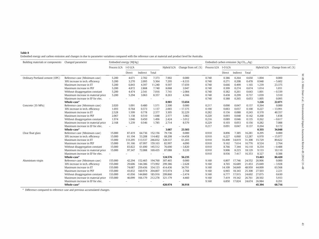
Table 8Embodied energy and carbon emission and changes in due to parameter variations compared with the reference case at material and product level for Australia.

Building materials or components Changed parameter Embodied energy (MJ/kg) Embodied carbon emission (kg CO2-e/kg)

Process LCA I-O LCA Hybrid LCA Change from ref. (%) Process LCA I-O LCA Hybrid LCA Change from ref. (%)

Direct Indirect Total Direct Indirect Total

Ordinary Portland cement (OPC) Reference case (Minimum case) 5.200 4.671 2.702 7.373 7.902 0.000 0.740 0.386 0.264 0.650 1.004 0.00030% increase in tech. efficiency 5.200 3.270 2.095 5.364 7.295 −8.333 0.740 0.271 0.208 0.478 0.948 −5.602Maximum increase in ET 5.200 6.843 4.397 11.240 9.597 17.659 0.740 0.666 0.499 1.165 1.239 23.375Maximum increase in PEF 5.200 4.872 2.868 7.740 8.068 2.047 0.740 0.399 0.274 0.674 1.014 1.031Without disaggregation constant 5.200 4.474 2.541 7.016 7.741 −2.084 0.740 0.382 0.261 0.643 1.001 −0.339Maximum increase in material price 5.200 5.294 3.063 8.357 8.263 4.366 0.740 0.438 0.299 0.737 1.039 3.510Maximum increase in EF for elec. – – – – – – 0.740 0.388 0.265 0.653 1.005 0.095Whole-casea 8.981 13.654 1.226 22.071

Concrete (35 MPa) Reference case (Minimum case) 2.020 1.091 0.480 1.571 2.500 0.000 0.217 0.090 0.047 0.137 0.264 0.00030% increase in tech. efficiency 1.693 0.764 0.373 1.137 2.065 −17.375 0.190 0.063 0.037 0.100 0.227 −13.991Maximum increase in ET 2.528 1.599 0.778 2.377 3.305 32.229 0.282 0.156 0.088 0.243 0.370 40.357Maximum increase in PEF 2.067 1.138 0.510 1.648 2.577 3.082 0.220 0.093 0.048 0.142 0.268 1.838Without disaggregation constant 1.974 1.046 0.450 1.496 2.424 −3.012 0.216 0.089 0.046 0.135 0.262 −0.617Maximum increase in material price 2.168 1.239 0.546 1.785 2.714 8.579 0.229 0.103 0.053 0.156 0.282 7.088Maximum increase in EF for elec. – – – – – – 0.217 0.091 0.047 0.137 0.264 0.172Whole-casea 3.087 23.503 0.355 34.848

Clear float glass Reference case (Minimum case) 15.000 87.419 64.736 152.156 79.736 0.000 0.910 8.896 7.385 16.281 8.295 0.00030% increase in tech. efficiency 15.000 61.194 53.208 114.402 68.208 −14.458 0.910 6.227 6.060 12.287 6.970 −15.977Maximum increase in ET 15.000 133.295 113.537 246.832 128.537 61.203 0.910 16.490 14.819 31.308 15.729 89.622Maximum increase in PEF 15.000 91.166 67.997 159.163 82.997 4.090 0.910 9.162 7.614 16.776 8.524 2.764Without disaggregation constant 15.000 83.822 61.690 145.512 76.690 −3.820 0.910 8.766 7.344 16.110 8.254 −0.488Maximum increase in material price 15.000 97.347 72.088 169.435 87.088 9.220 0.910 9.906 8.223 18.129 9.133 10.110Maximum increase in EF for elec. – – – – – – 0.910 8.936 7.417 16.353 8.327 0.388Whole-casea 124.576 56.235 15.463 86.420

Aluminium virgin Reference case (Minimum case) 155.000 42.294 152.465 194.760 307.465 0.000 9.160 6.807 17.746 24.552 26.906 0.00030% increase in tech. efficiency 155.000 29.606 144.386 173.992 299.386 −2.628 9.160 4.765 16.689 21.453 25.849 −3.928Maximum increase in ET 155.000 74.687 259.436 334.123 414.436 34.791 9.160 14.109 34.849 48.959 44.009 63.568Maximum increase in PEF 155.000 43.832 160.974 204.807 315.974 2.768 9.160 6.965 18.343 25.308 27.503 2.221Without disaggregation constant 155.000 41.056 144.860 185.916 299.860 −2.474 9.160 6.777 17.915 24.692 27.075 0.630Maximum increase in material price 155.000 46.099 166.179 212.278 321.179 4.460 9.160 7.419 19.342 26.761 28.502 5.933Maximum increase in EF for elec. – – – – – – 9.160 6.850 17.824 24.674 26.984 0.291Whole-casea 420.974 36.918 45.394 68.716

a Difference compared to reference case and previous accumulated changes.

41W.-M

.-S.Wan

Omar

etal./EnvironmentalIm

pactAssessm

entReview49

(2014)31

–48

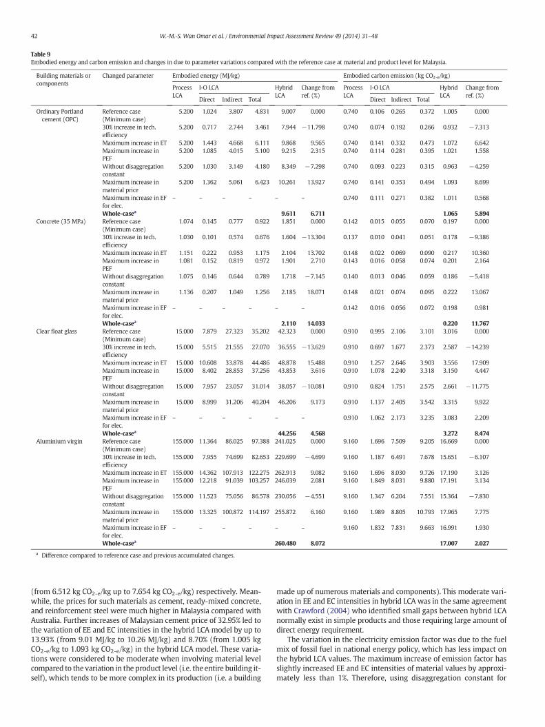
Table 9Embodied energy and carbon emission and changes in due to parameter variations compared with the reference case at material and product level for Malaysia.

Building materials orcomponents

Changed parameter Embodied energy (MJ/kg) Embodied carbon emission (kg CO2-e/kg)

ProcessLCA

I-O LCA HybridLCA

Change fromref. (%)

ProcessLCA

I-O LCA HybridLCA

Change fromref. (%)

Direct Indirect Total Direct Indirect Total

Ordinary Portlandcement (OPC)

Reference case(Minimum case)

5.200 1.024 3.807 4.831 9.007 0.000 0.740 0.106 0.265 0.372 1.005 0.000

30% increase in tech.efficiency

5.200 0.717 2.744 3.461 7.944 −11.798 0.740 0.074 0.192 0.266 0.932 −7.313

Maximum increase in ET 5.200 1.443 4.668 6.111 9.868 9.565 0.740 0.141 0.332 0.473 1.072 6.642Maximum increase inPEF

5.200 1.085 4.015 5.100 9.215 2.315 0.740 0.114 0.281 0.395 1.021 1.558

Without disaggregationconstant

5.200 1.030 3.149 4.180 8.349 −7.298 0.740 0.093 0.223 0.315 0.963 −4.259

Maximum increase inmaterial price

5.200 1.362 5.061 6.423 10.261 13.927 0.740 0.141 0.353 0.494 1.093 8.699

Maximum increase in EFfor elec.

– – – – – – 0.740 0.111 0.271 0.382 1.011 0.568

Whole-casea 9.611 6.711 1.065 5.894Concrete (35 MPa) Reference case

(Minimum case)1.074 0.145 0.777 0.922 1.851 0.000 0.142 0.015 0.055 0.070 0.197 0.000


1.030 0.101 0.574 0.676 1.604 −13.304 0.137 0.010 0.041 0.051 0.178 −9.386


1.081 0.152 0.819 0.972 1.901 2.710 0.143 0.016 0.058 0.074 0.201 2.164


1.075 0.146 0.644 0.789 1.718 −7.145 0.140 0.013 0.046 0.059 0.186 −5.418


1.136 0.207 1.049 1.256 2.185 18.071 0.148 0.021 0.074 0.095 0.222 13.067


– – – – – – 0.142 0.016 0.056 0.072 0.198 0.981

Whole-casea 2.110 14.033 0.220 11.767Clear float glass Reference case

(Minimum case)15.000 7.879 27.323 35.202 42.323 0.000 0.910 0.995 2.106 3.101 3.016 0.000


15.000 5.515 21.555 27.070 36.555 −13.629 0.910 0.697 1.677 2.373 2.587 −14.239


15.000 8.402 28.853 37.256 43.853 3.616 0.910 1.078 2.240 3.318 3.150 4.447


15.000 7.957 23.057 31.014 38.057 −10.081 0.910 0.824 1.751 2.575 2.661 −11.775


15.000 8.999 31.206 40.204 46.206 9.173 0.910 1.137 2.405 3.542 3.315 9.922


– – – – – – 0.910 1.062 2.173 3.235 3.083 2.209

Whole-casea 44.256 4.568 3.272 8.474Aluminium virgin Reference case

(Minimum case)155.000 11.364 86.025 97.388 241.025 0.000 9.160 1.696 7.509 9.205 16.669 0.000


155.000 7.955 74.699 82.653 229.699 −4.699 9.160 1.187 6.491 7.678 15.651 −6.107


155.000 12.218 91.039 103.257 246.039 2.081 9.160 1.849 8.031 9.880 17.191 3.134


155.000 11.523 75.056 86.578 230.056 −4.551 9.160 1.347 6.204 7.551 15.364 −7.830


155.000 13.325 100.872 114.197 255.872 6.160 9.160 1.989 8.805 10.793 17.965 7.775


– – – – – – 9.160 1.832 7.831 9.663 16.991 1.930

Whole-casea 260.480 8.072 17.007 2.027

a Difference compared to reference case and previous accumulated changes.


(from 6.512 kg CO2-e/kg up to 7.654 kg CO2-e/kg) respectively. Mean-while, the prices for such materials as cement, ready-mixed concrete,and reinforcement steel were much higher in Malaysia compared withAustralia. Further increases of Malaysian cement price of 32.95% led tothe variation of EE and EC intensities in the hybrid LCA model by up to13.93% (from 9.01 MJ/kg to 10.26 MJ/kg) and 8.70% (from 1.005 kgCO2-e/kg to 1.093 kg CO2-e/kg) in the hybrid LCA model. These varia-tions were considered to be moderate when involving material levelcompared to the variation in the product level (i.e. the entire building it-self), which tends to be more complex in its production (i.e. a building

made up of numerous materials and components). This moderate vari-ation in EE and EC intensities in hybrid LCA was in the same agreementwith Crawford (2004) who identified small gaps between hybrid LCAnormally exist in simple products and those requiring large amount ofdirect energy requirement.

The variation in the electricity emission factor was due to the fuelmix of fossil fuel in national energy policy, which has less impact onthe hybrid LCA values. The maximum increase of emission factor hasslightly increased EE and EC intensities of material values by approxi-mately less than 1%. Therefore, using disaggregation constant for

59

.00

0

67

.50

0

15

.00

0

3.0

00 5.2

00

2.0

20

6.7

50

28

.00

0

35

.40

0

15

5.0

00

38

.00

0

19

.77

0

12

.05

5

87

.41

9

2.3

57 4.6

71

1.0

91

0.9

60

56

.83

2

12

.65

0

42

.29

4

1.8

92

99

.95

1

58

.16

9

64

.73

6

1.2

03 2

.70

2

0.4

80

6.3

03

86

.03

6

13

.99

3

15

2.4

65

26

.91

3

11

9.7

21

70

.22

4 15

2.1

56

3.5

60 7.3

73

1.5

71

7.2

64

14

2.8

68

26

.64

3

19

4.7

60

28

.80

6

15

8.9

51

12

5.6

69

79

.73

6

4.2

03 7.9

02

2.5

00

13

.05

3

11

4.0

36

49

.39

3

30

7.4

65

64

.91

3

0.01

0.10

1.00

10.00

100.00

1,000.00

Em

bo

die

d e

ner

gy i

nte

nsi

ty (

MJ/

kg)

Process LCA Direct I-O LCA Indirect I-O LCA

Total I-O LCA Hybrid LCA

Fig. 6. Reference case of EE for different construction materials and products in Australia.


aggregated energy supply sector so that individual emission factor canbe used instead of average emission factor results in less variation inthe hybrid LCA model.

Whole-case combination of parameter changes

The analysis in the previous section considered the effect of varyingone parameter at a time and determined the changes in hybrid LCAresulting from changes to each parameter while maintaining all otherparameters constant. In this section, the whole-case scenario is alsoconsidered for this research and can be defined as the accumulatedchanges of all parameters on hybrid LCA variation as given in Tables 8and 9.

While all the parameter variations compared to the reference casesincreased the EE and EC intensities of materials and products in thehybrid LCA model, some parameter variations decreased EE and ECintensity values, which can be seen in both Australian and Malaysianmaterial intensities. Increase of technological efficiency and excludeddisaggregation constant reduced the variations of EE and EC intensitiesas shown in the Malaysianmaterial intensities. For example, increase of30% of concrete technology efficiency reduced 13.3% of EE intensityvalue in the hybrid LCA model.

To determine the effects of combined parameter variations, particu-larly those that could most affect the EE and EC intensities in the hybridLCAmodel, this research varied parameters tomakewhole-case scenar-io for both Australia andMalaysia by accumulating previous changes. Asshown in Tables 8 and 9, all previous changes from references cases (canbe positive or negative changes) were summed to quantify totalvariation of EE and EC intensities of materials and products. With thewhole-case combination of parameters for the hybrid LCA model, theimpacts on EE and EC intensities were classified into two categories:(1) impact on the non-energy intensive materials such as plasterboard,fibre glass insulation, and structural steel; and (2) impact on the energyintensive materials such as cement, steel, and clay brick. A high

variation in hybrid LCA model was observed with the whole-case sce-nario when applied to the non-energy intensive material that has highindirect energy and carbon emission intensities in the upstream bound-ary of the supply chain. These includematerials such as aggregates, clearfloat glass, structural steel, paints and fibre glass insulation (only select-ed materials were included in this paper). For example, for non-energyintensive materials such as clear float glass, the variation of all parame-ters significantly increased EE and EC intensity values from 79.74 MJ/kgto 124.58 MJ/kg and 8.295 kg CO2-e/kg to 15.463 kg CO2-e/kg, account-ing for 56.24% and 86.42% of the increase in hybrid LCA model forAustralia. Meanwhile, the variations of all parameters have less signifi-cant impact on energy intensive materials such as cement and claybrick which were largely influenced by the variation in process LCA.

While some parameter variations decreased hybrid LCA in compari-son to the referencematerial (e.g. 30% increase in technological efficien-cy and excluded disaggregation constant), high EE and EC intensityvariations in the hybrid LCA model were predominantly influenced bythe variations in technological changes (direct requirement coefficient),energy tariffs, and material prices. These key parameter variations aresignificantly impacted upon by materials or products with a high levelof indirect EE and EC, and are therefore considered a key issue in EEand EC methodology development. With regard to these variations,using highly aggregated industry sectors such as residential buildingto quantify specific types of building or modular or custom-designedstructures would increase EE and EC intensity variations of buildings.These results are in agreement with and provide contextual support toprevious studies (e.g. Dixit et al. (2013)).

Comparison with previous studies

This research compares the results from the hybrid LCA modeldeveloped in this research with previous researches based onAustralian, New Zealand and Malaysian I-O tables and the results aredepicted in Fig. 11. Selected building materials were classified into


energy and non-energy intensive materials that have different impactsdue to the parameter variations as mentioned in the previous sections.The comparison of EE and EC intensities of materials and productsacross models and countries found that energy intensive materialssuch as cement, clay brick and steel virgin are more consistent andshow less uncertainty and variation. This is due to the high proportionof process data that reduces uncertainty in the upstream boundary ofmaterials production (Lee andMa, 2013). More process data can reduceuncertainty and increase reliability in EE and EC intensities. Meanwhile,non-energy intensive materials with high indirect energy such as clearfloat glass, plasterboard, fibre glass insulation, plastic product andstructural steel vary significantly between the studied models. The re-sults showed that the EE intensities for clear float glass were 15.9 MJ/kg for New Zealand (Alcorn, 2003), 83.6 MJ/kg for Australia (Pullen,2007), 173.0 MJ/kg for Australia (Crawford, 2011), 97.47 MJ/kg forAustralia (Current study) and 46.05 MJ/kg for Malaysia (Currentstudy). All of these EE intensity values indicated significant variationsdue to parameter variations as previously discussed. (See Figs. 6-9.)

Incorporating these materials into EE and EC assessment would sig-nificantly impact the whole life cycle of a building and its components.Consequently, using hybrid LCAwith highly aggregated industry sectorssuch as residential construction would have a great influence on thevariations of a building's EE and EC. Baird et al. (1997) demonstratedthe changes in EE over a period of time and found that three quarterof EE intensities of materials and products drop an average of 41%whereas the remainder showed a rise averaging46%. He further demon-strated the significant effect of changes in material manufacturing tech-nology to the overall figure of a building, ranging from 32% to 56%.Unfortunately, the influences of parameter variations were not consid-ered in determining these changes.

The changes of technological efficiency, energy tariffs and materialprices caused not only significant variation in the country specific I-OLCA model but also led to variation between countries (multi regional

2.5

40

3.2

30

0.9

10

0.2

40

0.7

40

1.9

61

2.7

42

8.8

96

0.1

94 0

.38

6

10

.09

0

6.6

50

7.3

85

0.1

36 0

.26

4

12

.05

1

9.3

92 16

.28

1

0.3

30 0

.65

0

12

.63

0

9.8

80

8.2

95

0.3

76

1.0

04

0.01

0.10

1.00

10.00

100.00

Em

bo

die

d c

arb

on

in

ten

sity

(k

g C

O2

-e/k

g)

Process LCA Direct I-

Total I-O LCA Hybrid L

Fig. 7. Reference case of EC for different constru

I-O LCA such as Australia and Malaysia as previously discussed in Effectof parameter variations in hybrid LCA section andWhole-case combina-tion of parameter changes section.). As shown in Fig. 11, the results ofthis study clearly showed significant variation of hybrid LCA model be-tweenAustralia,Malaysia, andNewZealand. For instance, the variationsof EE intensities for UPVC pipe, clear float glass, plasterboard and struc-tural steel were significant due to the high amount of indirect energyand carbon embodied in upstream boundary of material production,accounted for more than 50% of total EE and EC (as previously shownin Tables 8 and 9 — only selected materials are presented in these ta-bles). Previous studies used the I-O LCA model to quantify all indirectimpacts caused by upstream products such as multi regional I-Omodel (MRIO) (Wiedmann et al., 2011).

MRIO model recently gain interest by research community to pro-vide methodological framework for complete EE and EC assessment atthe national and international level (Wiedmann, 2009; Wiedmannet al., 2011; Zhang et al., 2014). However, MRIO model inherits all un-certainties specific to single-region I-O LCA (country specific I-O LCA)which include uncertainties in source data, allocation, proportionalityand homogeneity, aggregation, temporal representativeness, modelinputs and multipliers. According to Wiedmann (2009), there are veryfew empirical studies on error estimates associated withMRIO analysis.Further, MRIO model is clearly an area that requires more attention byresearch community, including a high level evaluation of the proce-dures, findings, and evaluation across countries. Therefore, this paperprovides empirical findings to evaluate uncertainty of indirect EE andEC assessment which is more practical and less time consuming assuggested by Crawford (2004).

Discussion and conclusion

This research was conducted to identify factors that contribute mostsignificantly to the variation of embodied energy and carbon using the

0.2

17 0

.39

0

1.3

50

2.8

90

9.1

60

3.0

30

0.0

90

0.1

83

8.1

41

2.0

06

6.8

07

0.3

62

0.0

47

0.6

53

9.4

25

1.7

36

17

.74

6

3.4

82

0.1

37

0.8

36

17

.56

6

3.7

42

24

.55

2

3.8

44

0.2

64

1.0

43

10

.77

5

4.6

26

26

.90

6

6.5

12

O LCA Indirect I-O LCA

CA

ction materials and products in Australia.

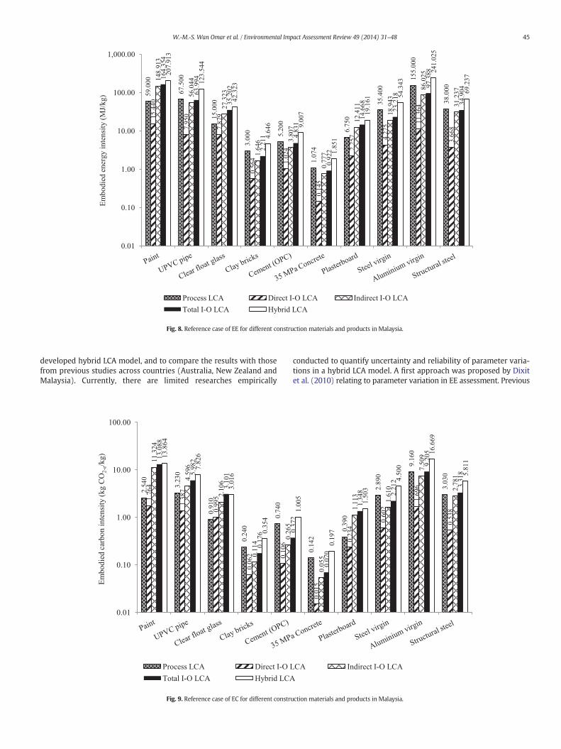
59

.00

0

67

.50

0

15

.00

0

3.0

00 5.2

00

1.0

74

6.7

50

35

.40

0

15

5.0

00

38

.00

0

15

.44

0

7.9

50

7.8

79

0.5

64 1.0

24

0.1

45

2.2

57 4.2

75

11

.36

4

3.6

68

14

8.9

13

56

.04

4

27

.32

3

1.6

46 3

.80

7

0.7

77

12

.41

1

18

.94

3

86

.02

5

31

.23

7

16

4.3

54

63

.99

4

35

.20

2

2.2

11 4

.83

1

0.9

22

14

.66

8

23

.21

8

97

.38

8

34

.90

4

20

7.9

13

12

3.5

44

42

.32

3

4.6

46 9.0

07

1.8

51

19

.16

1 54

.34

3

24

1.0

25

69

.23

7

0.01

0.10

1.00

10.00

100.00

1,000.00

Em

bo

die

d e

ner

gy i

nte

nsi

ty (

MJ/

kg)

Process LCA Direct I-O LCA Indirect I-O LCA


Fig. 8. Reference case of EE for different construction materials and products in Malaysia.


developed hybrid LCA model, and to compare the results with thosefrom previous studies across countries (Australia, New Zealand andMalaysia). Currently, there are limited researches empirically

2.5

40

3.2

30

0.9

10

0.2

40

0.7

40

1.7

64

1.3

87

0.9

95

0.0

62 0.1

06

11

.32

4

4.5

96

2.1

06

0.1

14

0.2

65

13

.08

8

5.9

82

3.1

01

0.1

76

13

.86

4

7.8

26

3.0

16

0.3

54

0.01

0.10

1.00

10.00

100.00

Em

bo

die

d c

arb

on

in

ten

sity

(k

g C

O2-e

/kg)

Process LCA Direct I-O L


Fig. 9. Reference case of EC for different constru

conducted to quantify uncertainty and reliability of parameter varia-tions in a hybrid LCA model. A first approach was proposed by Dixitet al. (2010) relating to parameter variation in EE assessment. Previous

0.1

42

0.3

90

2.8

90

9.1

60

3.0

30

0.0

15

0.2

34

0.6

02

1.6

96

0.5

38

0.0

55

1.1

13

1.6

10

7.5

09

2.7

81

0.3

72

0.0

70

1.3

48 2.2

12

9.2

05

3.3

18

1.0

05

0.1

97

1.5

03

4.5

00

16

.66

9

5.8

11

CA Indirect I-O LCA

ction materials and products in Malaysia.

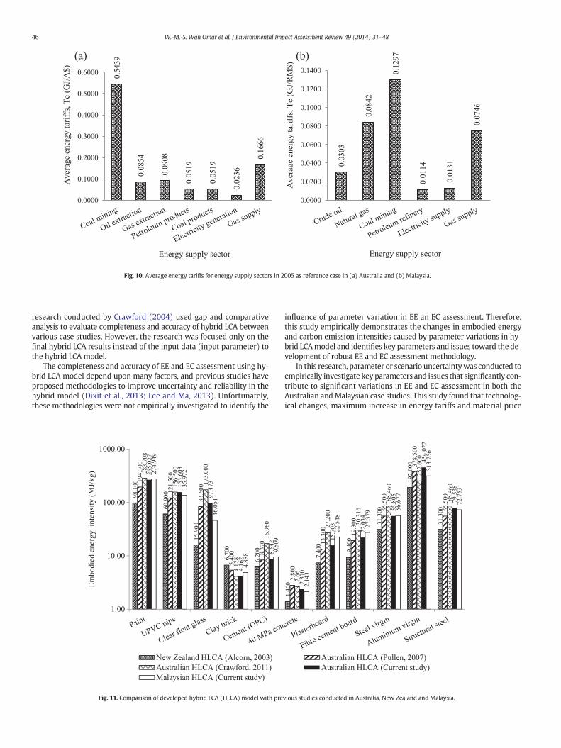
0.5

43

9

0.0

85

4

0.0

90

8

0.0

51

9

0.0

51

9

0.0

23

6

0.1

66

6

0.0000

0.1000

0.2000

0.3000

0.4000

0.5000

0.6000

(a) (b)A

ver

age

ener

gy t

arif

fs, T

e (G

J/A

$)

Energy supply sector

0.0

30

3

0.0

84

2

0.1

29

7

0.0

11

4

0.0

13

1

0.0

74

6

0.0000

0.0200

0.0400

0.0600

0.0800

0.1000

0.1200

0.1400

Aver

age

ener

gy t

arif

fs, T

e (G

J/R

M$)

Energy supply sector

Fig. 10. Average energy tariffs for energy supply sectors in 2005 as reference case in (a) Australia and (b) Malaysia.


research conducted by Crawford (2004) used gap and comparativeanalysis to evaluate completeness and accuracy of hybrid LCA betweenvarious case studies. However, the research was focused only on thefinal hybrid LCA results instead of the input data (input parameter) tothe hybrid LCA model.

The completeness and accuracy of EE and EC assessment using hy-brid LCA model depend upon many factors, and previous studies haveproposed methodologies to improve uncertainty and reliability in thehybrid model (Dixit et al., 2013; Lee and Ma, 2013). Unfortunately,these methodologies were not empirically investigated to identify the

98.1

00

60.9

00

15.9

00

6.70

0

6.20

0

194.

300

121.

500

83.6

00

5.40

0 8.37

0

283.

708

156.

500

173.

000

4.12

8

16.9

60

265.

027

155.

603

97.4

73

4.16

2

8.64

2

274.

949

135.

972

46.0

51

4.88

8 9.50

9

1.00

10.00

100.00

1000.00

Embo

died

ene

rgy

inte

nsity

(MJ/

kg)

New Zealand HLCA (Alcorn, 2003)Australian HLCA (Crawford, 2011)Malaysian HLCA (Current study)

Fig. 11. Comparison of developed hybrid LCA (HLCA) model with pre

influence of parameter variation in EE an EC assessment. Therefore,this study empirically demonstrates the changes in embodied energyand carbon emission intensities caused by parameter variations in hy-brid LCAmodel and identifies key parameters and issues toward the de-velopment of robust EE and EC assessment methodology.

In this research, parameter or scenario uncertaintywas conducted toempirically investigate key parameters and issues that significantly con-tribute to significant variations in EE and EC assessment in both theAustralian andMalaysian case studies. This study found that technolog-ical changes, maximum increase in energy tariffs and material price

1.40

0

7.40

0

9.40

0

31.3

00

192.

000

31.3

00

2.80

0

13.3

00 19.3

00

55.5

00

378.

500

55.5

00

2.66

1

27.2

00

30.3

16

85.4

60

252.

600

85.4

60

2.37

0

15.7

03 22.0

34

55.8

05

454.

022

79.5

38

2.14

3

22.5

48

27.3

79

56.6

77

313.

756

72.7

53

Australian HLCA (Pullen, 2007)Australian HLCA (Current study)

vious studies conducted in Australia, New Zealand and Malaysia.


fluctuation were the key parameters and issues leading to significantvariations in EE and EC intensity values. Other parameters such asmax-imum increase in primary energy factors, emission factors and exclud-ing disaggregation constants have slight impact upon EE and ECintensity variations.

When compared with previous studies across countries, the signifi-cant variations in EE and EC between energy and non-energy intensivematerials can be clearly seen due to the significant contribution of indi-rect energy in non-energy intensivematerial during production process.Building materials with high indirect energy in the upstream boundaryhave great influence on hybrid LCA variation between studies. There-fore, any decision relating to these materials should be considered care-fully. Thus one strategy to reduce uncertainty and increase reliability ofhybrid LCA data is by firstly calculating EE and EC intensities ofmaterialsand products and then computing EE and EC of the entire building byusing actual quantity of material, labour, and equipment (processLCA). This in turn can reduce the high variations of EE and EC intensityvalues caused by high dependency on aggregated industry sectors inthe I-O tables (e.g. residential and non-residential sector used inMalaysian I-O tables).

Study limitations and recommendations

This section outlines the general limitations of the current researchand makes recommendations regarding future research in the area ofEE and EC assessments:

• One limitation of the scope of the current study is that it onlyaddresses the building's embodied impact during the productionphase. Other phases were excluded from analysis due to reliabilityand validity concern on LCI data.

• The use of I-O data to roughly estimate EE and EC intensities of mate-rials, products and buildings has been investigated and evaluated ateach level of building construction (materials, product level up tobuilding level). There are lack of availability and quality of processdata for Australian and Malaysian building materials that preventthe specific process data of a product to be used in hybrid LCA.

• To improve the hybrid LCAmodel, the future research should attemptto increase availability of process data, particularly by conducting LCAfor particular materials and products. This in turn can increase theprecision of EE and EC calculation in process LCA (bottom-up analy-sis). Moreover, more research is needed to create a publicly availabledatabase locally so that further hybridisingprocesses between processLCA and I-O LCA can be smoothly conducted.

Acknowledgement

We gratefully acknowledge the financial support of the Ministry ofHigher Education (MoHE), Malaysia and Universiti Malaysia Perlis(UniMAP). We thank an anonymous reviewer for their valuable com-ment and feedback.

References

Acquaye AA. A stochastic hybrid embodied energy and CO2_eq intensity analysis of build-ing and construction processes in Ireland [Doctoral Thesis] Dublin: Dublin Institute ofTechnology (DIT), Ireland; 2010.

Acquaye AA, Duffy AP. Input–output analysis of Irish construction sector greenhouse gasemissions. Build Environ 2010;45:784–91.

Acquaye A, Duffy A, Basu B. Embodied emissions abatement - A policy assessment usingstochastic analysis. Energy Policy. 2011;39:429–41.

Alcorn A. Embodied Energy and CO2 Coefficients for New Zealand Building Materials. In:Report CfBPR, editor. Wellington, New Zealand: Victoria University of Wellington;2003.

Alvarez-Gaitan JP, Peters GM, Rowley HV, Moore S, Short MD. A hybrid life cycle assess-ment of water treatment chemicals: an Australian experience. Int J Life Cycle Assess2013:1–11.

Australian Bureau of Statistics. Australian and New Zealand Standard Industrial Classifica-tion 2006 (ANZSIC 2006). Australia: Australian Bureau of Statistics (ABS); 2006.

Baird G, Alcorn A, Haslam P. The energy embodied in building materials — updated NZcoefficients and their significance. IPENZ Transactions. Wellington, N.Z.: Institutionof Professional Engineers New Zealand; 1997. p. 89–94.

Basbagill J, Flager F, Lepech M, Fischer M. Application of life-cycle assessment to earlystage building design for reduced embodied environmental impacts. Build Environ2013;60:81–92.

Börjesson P, Gustavsson L. Greenhouse gas balances in building construction: woodversus concrete from life-cycle and forest land-use perspectives. Energy Policy2000;28:575–88.

Crawford RH. Using input–output data in life cycle inventory analysis [PhD]. Victoria,Australia: Deakin University; 2004.

Crawford RH. Validation of the use of Input–Output data for embodied energy analysis ofthe Australian construction industry. J Constr Res 2005;6:71–90.

Crawford RH. Life cycle assessment in the built environment. GB: Spon (E&F); 2011.Crawford RH, Treloar GJ. Validation of the use of Australian input–output data for building

embodied energy simulation. In: Augenbroe, Godfried, Hensen, Jan LM, editors. Build-ing Simulation 2003 (8th: 2003: Eindhoven, Netherlands)Eindhoven: NetherlandsOrganising Committee Building Simulation; 2003. p. 235–42.

Crawford RH, Czerniakowski I, Fuller RJ. A comprehensive framework for assessingthe life-cycle energy of building construction assemblies. Archit Sci Rev 2010;53:288(9).

Dixit MK, Fernández-Solís JL, Lavy S, Culp CH. Identification of parameters for embodiedenergy measurement: a literature review. Energy Build 2010;42:1238–47.

Dixit MK, Culp CH, Fernández-Solís JL. System boundary for embodied energy inbuildings: a conceptual model for definition. Renew Sustain Energy Rev 2013;21:153–64.

González B, Adenso-Dı ́az B, González-Torre P. LA fuzzy logic approach for the impactassessment in LCA. Resour Conserv Recycl 2002;37:61–79.

Gustavsson L, Sathre R. Variability in energy and carbon dioxide balances of wood andconcrete building materials. Build Environ 2006;41:940–51.

Gutowski TG. The carbon and energy intensity of manufacturing. 40th CIRP InternationalManufacturing Systems SeminarUK: Liverpool University; 2007.

Heijungs R. Identification of key issues for further investigation in improving the reliabil-ity of life-cycle assessments. J Cleaner Prod 1996;4:159–66.

Huijbregts MAJ, Norris G, Bretz R, Ciroth A, Maurice B, Bahr B, et al. Framework formodelling data uncertainty in life cycle inventories. Int J Life Cycle Assess 2001;6:127–32.

Huijbregts MAJ, Gilijamse W, Ragas AMJ, Reijnders L. Evaluating uncertainty in environ-mental life-cycle assessment. A case study comparing two insulation options for aDutch one-family dwelling. Environ Sci Technol 2003;37:2600–8.

International Energy Agency. Power generation from coal: measuring and reporting effi-ciency performance and CO2 emissions. France: International Energy Agency; 2010.

John Rawlinson Co-Partnership G. Rawlinson's Australian construction handbook.Brisbane, Qld: Rawlhouse Publishing; 2008.

Lee CH, Ma HW. Improving the integrated hybrid LCA in the upstream scope 3 emissionsinventory analysis. Int J Life Cycle Assess 2013;18:17–23.

LenzenM. Errors in conventional and input–output-based life-cycle inventories. J Ind Ecol2000;4:127–48.

Lenzen M, Dey C. Truncation error in embodied energy analyses of basic iron and steelproducts. Energy 2000;25:577–85.

Lenzen M, Treloar G. Embodied energy in buildings: wood versus concrete—reply toBörjesson and Gustavsson. Energy Policy 2002;30:249–55.

Lenzen M, Murray SA, Korte B, Dey CJ. Environmental impact assessment including indi-rect effects — a case study using input–output analysis. Environ Impact Assess Rev2003;23:263–82.

Malaysian Department of Statistics. Malaysia Standard Industrial Classification 2000(MSIC 2000). Kuala Lumpur, Malaysia: Malaysian Department of Statistics; 2000.

Malaysian Department of Statistics. Comparison of Malaysian economic structure, 2000 &2005. Malaysia: Department of Statistics; 2010.

Mongelli I, Suh S, Huppes G. A structure comparison of two approaches to LCA inventorydata, based on the MIET and ETH databases. Int J Life Cycle Assess 2005;10:317–24.

Nässén J, Holmberg J, Wadeskog A, Nyman M. Direct and indirect energy use and carbonemissions in the production phase of buildings: an input–output analysis. Energy2007;32:1593–602.

Price L, du Can SdlR, Sinton J, Worrell E, Nan Z, Sathaye J, et al. Sectoral trends in globalenergy use and greenhouse gas emissions. Environmental Energy TechnologiesDivision: Lawrence Berkeley National Laboratory; 2006.

Pullen SF. The spatial representation of embodied energy of residential areas in the urbanenvironment [PhD]. Adelaide, Australia: The University of Adelaide; 2007.

Shipworth D. A stochastic framework for embodied greenhouse gas emissions modellingof construction materials. Build Res Inf 2002;30:16–24.

Suh S, Huppes G. Methods for life cycle inventory of a product. J Cleaner Prod 2005;13:687–97.

Suh S, LenzenM, Treloar GJ, Hondo H, Horvath A, Huppes G, et al. System boundary selec-tion in life-cycle inventories using hybrid approaches. Environ Sci Technol 2003;38:657–64.

Treloar GJ. A comprehensive embodied energy analysis framework [PhD] Australia:Deakin University; 1998.

Treloar GJ, Love PED, Faniran OO, Iyer-Raniga U. A hybrid life cycle assessment method forconstruction. Constr Manag Econ 2000;18:5–9.

Wan OmarWMS, Doh JH, Panuwatwanich K. Assessment of embodied energy and carbonemission of building and construction processes in Malaysia using process-basedhybrid analysis. In: Vimomsatit V, Singh A, Yazdani S, editors. The First Australasiaand South East Asia Conference in Structural Engineering and Construction (ASEA-SEC-1). Curtin University, Perth, Western Australia: Research publishing services;2012. p. 803–7.

http://refhub.elsevier.com/S0195-9255(14)00055-9/rf0190








































































































48 W.-M.-S. Wan Omar et al. / Environmental Imp

Wan OmarWMS, Doh JH, Panuwatwanich K. Variability in assessment of embodied ener-gy and carbon material intensity using Hybrid LCA: Malaysian experience. 3rd Inter-national Conference and Exhibition on Sustainable Energy and Advanced Material(ICE-SEAM 2013)Melaka, Malaysia: Melaka International Trade Centre; 2013.

Wan Omar WMS, Doh JH, Panuwatwanich K, Miller D. Assessment of the embodied car-bon in precast concrete wall panels using a hybrid life cycle assessment approach inMalaysia. Sustain Cities Soc 2014;10:101–11.

Wiedmann T. A review of recent multi-region input–output models used forconsumption-based emission and resource accounting. Ecol Econ 2009;69:211–22.

Wiedmann T, Wilting HC, Lenzen M, Lutter S, Palm V. Quo Vadis MRIO? Methodological,data and institutional requirements for multi-region input–output analysis. Ecol Econ2011;70:1937–45.

Williams ED, Weber CL, Hawkins TR. Hybrid framework for managing uncertainty in lifecycle inventories. J Ind Ecol 2009;13:928–44.

Zhang B, Li J, Peng B. Multi-regional input–output analysis for China's regional CH4

emissions. Front Earth Sci 2014;8:163–80.

Wan Mohd Sabki Wan Omar is PhD candidate in the School of Engineering at GriffithUniversity, Gold Coast Campus, Australia. He obtained Bachelor of Engineering (Honours)(Civil Engineering) from Universiti Teknologi Malaysia (UTM) and obtained Master of En-gineering (Construction Engineering and Management) from Asian Institute of Technology(AIT), Bangkok, Thailand. His current research interest focus is on sustainable construction,life cycle energy and carbon assessment, and embodied energy and carbon assessment inconstruction.

Dr. Jeung-Hwan Doh is a Senior Lecturer in the School of Engineering at GriffithUniversity, Gold Coast Campus, Australia. He obtained Bachelor of Honours and Masterof Honours in his civil engineering degree from University of Wollongong and obtainedPh.D. from Griffith University. His current research focus is on reinforced concrete walls,slabs, construction material embodied energy consumption and sustainable design meth-od for concrete structures.

Dr. Kriengsak Panuwatwanich is Senior Lecturer in Engineering and ProjectManagement at Griffith School of Engineering, Griffith University, Queensland, Australia.He obtained his Bachelor's degree (Civil Engineering) from Thammasat University inThailand, a Master of Engineering Science (Engineering Construction and Management)from the University of New South Wales and a Ph.D. from Griffith University, Australia.He has been an academic since 2000. His teaching areas and research interests encompassthe fields of engineering, construction and project management, as well as engineeringeducation. He also serves as Chair of Engineers Australia Gold Coast Regional Group.

act Assessment Review 49 (2014) 31–48

















variations in embodied energy and carbon emission intensities of construction materials

Documents