Varieties of Capitalism: The Flexicurity Model

Peter Flaschel,∗ Alfred Greiner,

Department of Economics and Business Administration,Bielefeld University, Bielefeld, Germany

Sigrid Luchtenberg

Department of EducationUniversity of Duisburg – Essen, Essen, Germany

Edward NellDepartment of Economics, Graduate Faculty

New School for Social Research, New York, USA

Running head: Flexicurity Capitalism.

June 15, 2007

∗Corresponding author. Email: pflaschel@wiwi.uni-bielefeld.de. We have to thank the participantsof seminars held in Chemnitz University, Bielefeld University and the IMK, Dusseldorf and in particularGangolf Groh for very helpful suggestions that improved the paper significantly. Of course, usual caveatsapply.

1

2

Abstract

We start from the finding that Goodwin’s (1967) growth cycle model, i.e.,the Marxian reserve army mechanism, does not represent a process of social re-production that can be considered an adequate socio-economic foundation for ademocratic society in the long-run. The paper then derives a basic macrodynamicframework where this distinct form of cyclical growth and social reproductionis overcome by an employer of ’first’ resort, added to an economic reproductionprocess that is highly competitive and thus not of the type of the past Eastern so-cialism. There is high labor and capital mobility (concerning ’hiring’ and ’firing’in particular) where fluctuations of employment in the private sector are madesocially acceptable through a second labor market where all remaining workersget occupation and income. The resulting socio-economic system is closely relatedto the flexicurity model developed for Denmark in particular. We show that thiseconomy exhibits a balanced growth path that is globally attracting. Moreover,pension-fund financed investment can be added to this model without disturbingthe prevailing situation of stable full capacity growth The closing section showshowever that a paper credit formulation of this process can lead to Keynesianeffective demand constraints in this type of economy.

Keywords: Distributive growth cycles, employer of first resort, stable balancedgrowth, supply-driven business fluctuations.

JEL classifications: E32, E64, H11.

3

Contents

1 Social reproduction and the reserve army mechanism 4

2 Flexicurity growth: A baseline model 9

3 Goodwin-Kalecki dynamics: Progress towards consent economies andbeyond? 13

4 Flexicurity growth: Full capacity convergence towards balanced repro-duction 184.1 The dynamics and their balanced growth path . . . . . . . . . . . . . . . 184.2 Monotonic convergence towards balanced growth . . . . . . . . . . . . . . 204.3 Global viability . . . . . . . . . . . . . . . . . . . . . . . . . . . . . . . . 21

5 Company pension funds: Dynamics and steady state levels 22

6 Pension funds and credit 246.1 Accounting relationships . . . . . . . . . . . . . . . . . . . . . . . . . . . 246.2 Investment and credit dynamics in flexicurity growth . . . . . . . . . . . 27

7 Outlook: Keynesian demand problems 30

References 35

4

1 Social reproduction and the reserve army mecha-

nism

This paper starts from the observation that Goodwin’s (1967) Classical growth cycledoes not represent a process of social reproduction that can be considered as adequatefor a social and democratic society in the long-run. The paper therefore derives on thisbackground a basic macrodynamic framework where this form of cyclical growth andsocial reproduction is overcome by an employer of ’first’ resort, added to an economicreproduction process that is highly competitive and flexible and thus not of the type ofthe past Eastern socialism. Instead, there is high capital and labor mobility (concerning’hiring’ and ’firing’ in particular) where fluctuations of employment in the first labormarket of the economy (in the private sector) are made socially acceptable through asecond labor market where all remaining workers (and even pensioners) find meaningfuloccupation. The resulting economic system with its detailed transfer payment schemes isin its essence comparable to the flexicurity model developed for the Nordic welfare statesand Denmark in particular. We show that this economy exhibits a balanced growth paththat is globally attracting. Moreover, credit financed investment can be easily addedwithout disturbing the prevailing situation of full capacity growth. We thus do not getdemand-, but only supply-driven business fluctuations in such an environment with bothfactors of production always full employed. This combines flexible factor adjustment inthe private sector of the economy with high employment security for the labor force andthus shows that the flexicurity variety of capitalist reproduction can work in a balancedor at least fairly stable manner.We start from the (in 1995) still weak empirical evidence for the existence of a long-phase cycle in the state variables e and v, the employment rate and the wage share, thatwe have presented in Flaschel and Groh (1995) for a number of industrialized marketeconomies. We do this on the basis of fifteen years of further observations and now alsopartly based on quite modern econometric techniques. Our brief findings will be thatthe Goodwin growth cycle model of Flaschel and Groh (1995) provides indeed a usefulapproach to the explanation of the distributive cycle as it was observed in the US, theUK and in other countries after World War II. In Kauermann et al. (2007) we haveobtained by specifically tailored econometric techniques the graphical representationof the long-phase wage share v / employment rate e cycle (as centers of the businessfluctuations around them) for the U.S. economy over the period 1955 – 2004. Figure 1shows (bottom-right) a single estimated long-phase core cycle (within the scatter plot ofv, e−observations) for a period length of approximately 50 years and (bottom-left) the6-7 cycles of business cycle frequency (approximately 8 years each) that fluctuate aroundthis long-phase cycle. We ignore the shorter cycles in the following and concentrate onthe observation that there is evidence for a long-phase overshooting (non-monotonic)interaction between the share of wages v in national income and the employment rate e,the core of which is shown in figure 1, bottom right. This clockwise oriented long-phasecycle appears to be more complex in situations of a high employment rate and is relativelysimple structured in the opposite situations. The reader is referred to Kauermann etal. (2007) for details on the applied econometric technique and the results that can beobtained from it.

5

Figure 1: Goodwinian wage share / employment rate dynamics (bottom plots) withestimated long-phase cycle to the right. Top graphs show the data plotted against time.

In order to briefly present a simple model of such a long-phase accumulation cycle in thevariables v and e we make use of the seminal growth cycle model of Goodwin (1967).From this perspective, the envisaged cycle-generating feedback structure can be basedon the following two laws of motion:

v = v/v = βve(e − e) − βvv(v − v), (1)

e = e/e = −βev(v − v), (2)

where v denotes real unit-wage costs (or the share of wages in GDP) and e the em-ployment rate and the parameters βve > 0, βev > 0, βvv ≥ 0 determine the speed ofadjustment. The coefficients e and v denote the normal levels of employment and thewage share, respectively, meaning that employment and the wage share are constant at

6

those values. We justify eq. (1) by means of the wage dynamics investigated in Blan-chard and Katz (1999), with perfect anticipation of price inflation however (implying areal wage Phillips curve) where in addition to demand pressure we have unit wage costsacting as an error correction mechanism on their own evolution. In the second law ofmotion we focus on a goods market behavior that is profit-led, i.e., increases in unitwage costs act negatively on aggregate demand and thus negatively on the growth rateof the rate of employment e.If βvv = 0 holds, as Blanchard and Katz assert it for the U.S. economy, we have thecross-dual dynamics of the Goodwin (1967) growth cycle model and thus a center typedynamics that is stable, but not asymptotically stable. In the case βvv > 0 we can applyOlech’s Theorem, see Flaschel (1984), and obtain from it global asymptotic stability ofthe dynamics in the positive orthant of the phase plane with respect to the uniquelydetermined interior steady state position e, v. For weak Blanchard and Katz (1999)error correction terms we thus get a somewhat damped long-phased cyclical motion inthe wage share / employment rate phase space as shown in figure 2. We have a clockwiserotation in the considered phase space with approximately one cycle in 50 years.1

We can see that the theoretical 2D dynamics mirrors the empirical phase plot to a cer-tain degree. The Goodwin growth cycle mechanism where employment growth dependsnegatively on income distribution (is profit-led) and where wage share growth dependspositively on the state of the labor market thus not only explains the clockwise orienta-tion observed in the data, but also the long-phased nature of the cycle when adjustmentspeeds are crudely chosen from an empirical perspective. The unique observation of asingle long cycle in income distribution and employment that we have available for theU.S. economy after World War II is thus in fairly close correspondence to the Classicalgrowth cycle model and its suggestion of a long-phase accumulation cycle.2

Generating order and economic viability in market economies by large swings in theunemployment rate (mass unemployment with human degradation of part of the familiesthat form the society), as shown above (see also the next figure on the growth cyclestructure in the British economy), is one way to make capitalism work, but it mustsurely be critically reflected with respect to its social consequences. Moreover, it mustbe contrasted with alternative economic systems that allow to combine the situation of ahighly competitive market economy with a human rights bill that includes the right (andthe obligation) to work, and to get income from this work that at the least supports basicneeds and basic happiness. The Danish flexicurity system provides a typical examplefor such an alternative. By contrast, a laissez-faire capitalistic society that ruins familystructures to a considerable degree (through alienated work, mass unemployment andunlimited media programs) cannot stay a democratic society in the long-run, since it

1The parameters underlying this simulation are: βve = 0.06; e = 0.9; βvv = 0.01; βev = 0.1; v = 0.6.

and are approximately obtained from simple OLS estimates of these dynamics (with no good statisticalproperties however, but definitely more appropriately chosen compared to the case without any empiricalreference).

2Note with respect to figure 2 that it is assumed there that an increasing wage share is accompaniedby inflationary pressure as it is suggested by the conflicting income claims approach. Note furthermorethat – as is shown in Flaschel, Tavani, Taylor and Teuber (2007) – this cycle can be more complicatedin nature if empirically observed nonlinearities in the money wage Phillips curve are taken into accountwhich in fact move the cycle of the theoretical model already fairly close to what is shown in figure 1,bottom right.

7

produces conflicts that can range from social segmentation to class clashes, racial clashesand more.

e

v

Stagflation

DepressionRecovery

Prosperity Phase

1960's 1970's

1980's1990's

Figure 2: Goodwin-type long-phased wage share / employment dynamics

In addition to what has been shown above, one should, of course also try to take earliertime periods into account than just the 1960’s to the present if data – in particular on thewage share – are available. For the United Kingdom we have considered in Flaschel andGroh (1995) such long time–series from 1855 up to 19653 which can here be extendedto the following phase plot diagram.4

The important insight that can be obtained from these diagrams for Great Britain (1855– 1965) is that the Goodwin cycle – if it really existed – must have been significantlyshorter before 1914 (with larger fluctuations in employment during each business cycle),and that there has been a major change in it after 1945. This may be explained bysignificant differences and changes in the adjustment processes of market economiesfor these two periods: primarily price adjustment before 1914 and primarily quantityadjustments after 1945. This very tentative judgment must be left for future researchhere however. Based on Desai’s data one could have expected that the growth cycle hadbecome obsolete (and maybe also the business cycle as it was claimed in the 1960’s).Yet, extended by the further data from Groth and Madsen (2007), it is now of courseobvious that nothing of this sort took place in the UK economy. In fact, we see in figure3 two periods of excessive employment (in the language of the theory of the NAIRU)which were followed by periods of dramatic unemployment, both started by segmentsthe more or less pronounced occurrence of stagflation.Such a long-run perspective allows to see to what extent the above shown cycle for theUS economy is of a unique nature and therefore possibly representing a specific stage

3See Desai(1984) for the sources of these data and for an econometric approach on the basis of thesedata with respect to the Goodwin growth cycle model.

4We have to thank C. Groth and J. Madsen for providing access to these data, they have collected fortheir paper on ‘Medium-term fluctuations and the ”Great Ratios” of economic growth” (unpublished).

8

0.80

0.84

0.88

0.92

0.96

1.00

.40 .44 .48 .52 .56 .60 .64 .68 .72

UKWS

UKER

1

1870 1914−

2004

1945 1965−

1932

1975

1985

Figure 3: UK Income Distribution Cycles 1870 –2004: WS = wage share, ER = employ-ment rate

in the social structure of accumulation of capitalist market economies. As the figure 3shows there are indeed two such phases visible in the case of the United Kingdom whichare clearly separated from each other through the period where World War I and II weretaking place. In Flaschel and Groh (1995) we had a long time series from 1855 up to 1965which when taken in isolation could have suggested what was articulated at that time as’is the business cycle obsolete’ (Bronfenbrenner, 1969). When Flaschel and Groh (1995)was published the time-bound illusion in such a statement was of course already obvious,yet it is interesting to see (in figure 3) how radically this illusion was disproved by thedevelopment that took place in the UK after 1965. There is a Goodwinian distributivecycle after World War II in the UK and it implies the question of what we will observein this regard in the next 50 years in the UK and elsewhere.From the perspective of the flexicurity model that we will formulate and investigatein this paper the phase plot in figure 3 in our view clearly suggests that the depictedevolution in the British economy cannot be considered as an ideal for the next stage ofthe evolution of capitalism. Instead, we will pursue in this paper the idea that there isa coherent and workable alternative to the depicted distributive cycle in a competitivemarket environment that mirrors partial as well as macro ideas of the current discus-sion on the conduct of in particular labor market policies, in particular in the Nordiccountries.In the next section, we augment the Goodwin model by a second labor market wherethe state acts as the employer of ’first’ resort5 and thus guarantees full employment byspecific actions. We show that this extension not only removes the reserve army mecha-nism from the labor market, despite the possibility of a wage-price spiral mechanism inthe first labor market, but also makes the economy convergent to its long-run balanced

5and thus not yet of last resort, since this latter approach has been rightly criticized as being toopassive and inventory like in nature.

9

growth path and this the faster the more flexible the labor market is adjusting. Apartfrom the (important) microeconomic problem of how the second labor market that ishere added to the Goodwin growth cycle model can work in an efficient and socially ac-ceptable manner we thus get the result that the macroeconomic performance is not onlyimproved by this reformulation of the Goodwin model, but indeed turned into a statethat can be considered as socially superior to the actual working of capitalist marketeconomies like the USA and the UK.

2 Flexicurity growth: A baseline model

We have considered from the theoretical and the empirical perspective a long phasegrowth cycle that in the theoretical model of Flaschel and Groh (1995) was based – asmodification of the simple Goodwin growth cycle approach discussed in the precedingsection – on a repelling steady state and behavioral nonlinearities far off the steadystate that tame the explosive dynamics and turn it viable and that is confirmed in itsqualitative features through econometric measurements for the US economy after WorldWar II. This reserve army mechanism, the distributive cycle as well as the accompanyinginflation / unemployment cycle, is obviously a fairly archaic way to provide boundednessand order in a advanced capitalist market economy and its democratic institutions. Weare therefore now designing as an alternative to the preceding one a growth model thatrests in place of overaccumulation (in the prosperity phase) and mass unemployment(in the stagnant phase) on a second labor market which through its institutional setupguarantees full employment in its interaction with the first labor market, the employmentin the industrial sector of the economy that is modelled as highly flexible and competitive.We therefore first reconsider the sector of firms in such an economy:

Firms

Production and Income Account:Uses Resources

δK δKω1L

d1, Ld

1 = Y p/z C1 + C2 + Cr

ω2Lw2f G

Π (= Y f) I (= Y f)

δ1R + R S1

Y p Y p

This account is a very simple one. Firms use their capital stock (at full capacity uti-lization as we shall show later on) to employ the amount of labor (in hours): Ld

1 inits operation, at the real wage ω1, the law of motion of which is to be determined inthe next section from a model of the wage-price level interaction in the manufacturingsector. They in addition employ labor force Lw

2f = αfLd1, αf = const from the second

labor market at the wage ω2, which is a constant fraction αω of the market wage inthe first labor market. This labor force Lw

2f is working the normal hours of a standard

10

workday, while the workforce Lw1 from the first labor market may be working overtime

or undertime depending on the size of the capital stock in comparison to its own size.The rate uw = Ld

1/Lw1 is therefore the utilization rate of the workforce in the first labor

market, the industrial workers of the economy (all other employment comes from theworking of households occupied in the second labor market). Note finally, that in linewith the model of section, we allow for capital stock depreciation at the rate δ.Firms produce full capacity output6 Y p + δ1R = C1 + C2 + Cr + I + δK + G, that issold to the two types of consumers (and the retired households), the investing firms andthe government. The demand side of the model is formulated here in a way such thatindeed this full capacity output can be sold in this way, see the next section on thismatter. Deducting from this output and income Y p of firms their real wage paymentsto workers from the first and the second labor market (and depreciation)7 we get theprofits of firms which are here assumed to be invested fully into capital stock growthK = I = Π. We thus have Classical (direct) investment habits in this basic approachto a model with an employer of first resort. There is therefore not yet debt or equityfinancing of investment in this model type.We assume a fixed proportions technology with yp = Y p/K the potential output – capitalratio and with z = Y p/Ld

1 the given value of labor productivity (which determines theemployment Ld

1 of the workforce Lw1 of firms).

We next consider the households sector of our social growth model which is composedof worker households working in the first labor market and the remaining ones that areall working in the second labor market.

Households I and II (primary and secondary labor market)

Income Account (Households I):Uses Resources

C1 = ch1(1 − τh)ω1Ld1

ω2Lw2h = ch2(1 − τh)ω1L

d1

T = τhω1Ld1

ω2(L − (Lw1 + Lw

2f + Lw2h + Lw

2g))ω2L

r, Lr = αrLS1 ω1L

d1

Y w1 = ω1L

d1 Y w

1 = ω1Ld1

Income Account (Households II):Uses Resources

C2 ω2Lw2 , Lw

2 = L − Lw1

Y w2 Y w

2

Households of type I consume manufacturing goods of amount C1 and services from thesecond labor market Lw

2h. They pay an (all) income tax T and they pay in addition – via

6augmented by company pension payments δR.7the term S1 is equal to δ1R + R.

11

further tax transfers – all workers’ income in the labor market that is not coming fromfirms, from them and government (which is equivalent to an unemployment insurance).Moreover, they pay the pensions of the retired households (ω2L

r) and accumulate theirremaining income S1 in the form a company pension into a fund R that is administratedby firms (with inflow S1, see the sector of households and outflow δ1R).The transfer ω2(L−(Lw

1 +Lw2f +Lw

2h+Lw2g) can be considered as solidarity payments, since

workers from the first labor market that lose their job will automatically be employedin the second labor market where full employment is guaranteed by the government (asemployer of first resort). We consider this employment as skill preserving, since it canbe viewed as ordinary office or handicraft work (subject only to learning by doing whensuch workers return to the first labor market, i.e, employment in the production processof firms).The second sector of households is here modelled in the simplest way that is available:Households employed in the second labor market, i.e, Lw

2 = Lw2f + Lw

2h + Lw2g pay no

taxes and totally consume their income. We have thus Classical saving habits in thishousehold sector, while households of type 1 may have positive or negative savings S1 asresidual from their income and expenditures. We here assume that they can accumulatethese savings (or dissave in case of a negative S1) from the stock of commodities theyhave accumulated as inventories in the past.In order to have a consistent distribution of the funds R that are accumulated by house-holds of type I on the basis of their savings S1, according to the stock-flow relationshipR = S1 we have to modify this relationship as follows:

R = S1 − δ1R

where δ1 is the rate by which these funds are depreciated through company pensionpayments to the ’officially retired’ workers Lr assumed to be a constant fraction ofthe ’active’ workforce Lr = αrL. These worker households are added here as not reallyinactive, but offer work according to their still existing capabilities that can be consideredas an addition to the supply of work organized by the government L− (Lw

1 +Lw2f +Lw

2h),i.e., the working potential of the officially retired persons remains an active and valuablecontribution of the workhours that are supplied by the members of the society. It isobvious that the proper allocation of the work hours under the control of the governmentneeds thorough reflection from the microeconomic and the social point of view, whichhowever cannot be a topic in a paper on the macroeconomics of such an economy.As the income account of the retired households, shown below, shows they receive pen-sion payments as if they would work in the second labor market and they get in additionindividual transfer income (company pensions) from the accumulated funds R in pro-portion to the time they have been active in the first labor market and as an aggregatehousehold group of the total amount δ1R by which the pension funds R are reduced ineach period.

Income Account (Retired Households):Uses Resources

Cr ω2Lr + δ1R, Lr = αrL

Y r Y r

There is finally the government sector which is also formulated in a very basic way:

12

The Government

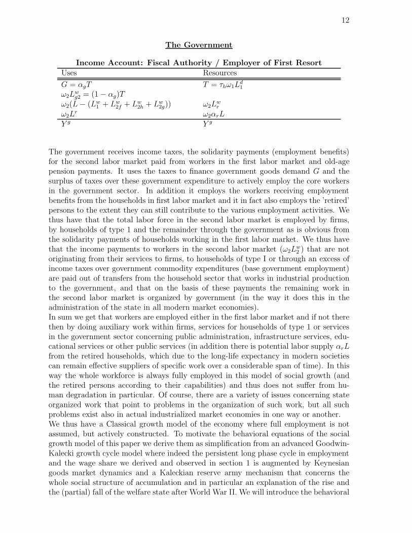
Income Account: Fiscal Authority / Employer of First ResortUses Resources

G = αgT T = τhω1Ld1

ω2Lwg2 = (1 − αg)T

ω2(L − (Lw1 + Lw

2f + Lw2h + Lw

2g)) ω2Lwr

ω2Lr ω2αrL

Y g Y g

The government receives income taxes, the solidarity payments (employment benefits)for the second labor market paid from workers in the first labor market and old-agepension payments. It uses the taxes to finance government goods demand G and thesurplus of taxes over these government expenditure to actively employ the core workersin the government sector. In addition it employs the workers receiving employmentbenefits from the households in first labor market and it in fact also employs the ’retired’persons to the extent they can still contribute to the various employment activities. Wethus have that the total labor force in the second labor market is employed by firms,by households of type 1 and the remainder through the government as is obvious fromthe solidarity payments of households working in the first labor market. We thus havethat the income payments to workers in the second labor market (ω2L

w2 ) that are not

originating from their services to firms, to households of type I or through an excess ofincome taxes over government commodity expenditures (base government employment)are paid out of transfers from the household sector that works in industrial productionto the government, and that on the basis of these payments the remaining work inthe second labor market is organized by government (in the way it does this in theadministration of the state in all modern market economies).In sum we get that workers are employed either in the first labor market and if not therethen by doing auxiliary work within firms, services for households of type 1 or servicesin the government sector concerning public administration, infrastructure services, edu-cational services or other public services (in addition there is potential labor supply αrLfrom the retired households, which due to the long-life expectancy in modern societiescan remain effective suppliers of specific work over a considerable span of time). In thisway the whole workforce is always fully employed in this model of social growth (andthe retired persons according to their capabilities) and thus does not suffer from hu-man degradation in particular. Of course, there are a variety of issues concerning stateorganized work that point to problems in the organization of such work, but all suchproblems exist also in actual industrialized market economies in one way or another.We thus have a Classical growth model of the economy where full employment is notassumed, but actively constructed. To motivate the behavioral equations of the socialgrowth model of this paper we derive them as simplification from an advanced Goodwin-Kalecki growth cycle model where indeed the persistent long phase cycle in employmentand the wage share we derived and observed in section 1 is augmented by Keynesiangoods market dynamics and a Kaleckian reserve army mechanism that concerns thewhole social structure of accumulation and in particular an explanation of the rise andthe (partial) fall of the welfare state after World War II. We will introduce the behavioral

13

equations of our social growth model by contrasting them – as we go along – withwhat has been assumed in Flaschel, Franke and Semmler (2007) within the Goodwin-Kaleckian growth cycle model of a distributive reserve army mechanism coupled withKalecki’s (1943) political aspects of full employment.

3 Goodwin-Kalecki dynamics: Progress towards

consent economies and beyond?

In this section we go on from the Goodwinian modeling of the Marxian reserve armymechanism to its extension as a Kaleckian model of the evolution of the welfare state afterWorld War II as it was modelled in Flaschel, Franke and Semmler (2007). We progressedin this framework from the case of dissent economies (where in fact a Goodwinian anda Kaleckian type of reserve army mechanism were interacting) to the case of consenteconomies where we could show the existence of a high and attracting balanced growthpath for such an economy. The following table 1 shows the range of possibilities thatwas considered in Flaschel, Franke and Semmler (2007).

high steady state low steady state

stable Nordic Kaleckian market economysteady state consent economy type I

unstable Kaleckian market economy Southernsteady state type II dissent economy

Table 1: Four types of market economies.

As conditions for the existence of a consent economy, we assumed Flaschel, Franke andSemmler (2007), see the behavioral equations below, that demand pressure in the labormarket (both inside and outside of the firm) does not influence the rate of wage inflationvery much, i.e., the wage level is a fairly stable magnitude. Furthermore, the Kaleckianreserve army mechanism was absent from the model (ie = 0). Moreover, the benchmarkvalues for demand pressures and the employment policy of firms are consistent with eachother and all sufficiently high to not imply labor market segmentation and significantdisqualification of unemployed workers. This can be coupled with flexible hiring andfiring policies then, i.e., the parameter βeu may be chosen as large as it is desirable.

This modified Kaleckian approach to consent economies is contrasted in the followingwith the dynamics and the balanced growth path of the model of flexicurity capitalism wehave introduced in the preceding section. We there compare models of the distributivegrowth cycle (with more or less conflict between capital and labor) with the flexicurityvariant of competitive capitalism. However, the important and difficult topic of thegeneration of socio-economic progress paths that lead from distributive conflict cycles toconsent economies and from there towards the proper functioning of an employer of firstresort economy, as the perspective of the flexicurity approach to social growth, must beleft for future research here.We derive the behavioral relationships of our model of flexicurity capitalism by con-trasting them with the Kaleckian growth cycle model of Flaschel, Franke and Semmler

14

(2007). We represent the laws of motion of the latter economy first in a framework ofGoodwin-Kalecki type, before we show how these equations simplify in our model ofsocial growth with an employer of first resort.We consider first the wage-price dynamics in the first labor market, which is the onlylabor market in the Goodwin-Kalecki approach. For the description of these dynamicswe start from a general formulation of a wage-price spiral as shown below, see Flaschel,Franke and Semmler (2007) for a detailed treatment of its structure.8

w = βwe(e − e) + βwu(uw − uw) − βwω ln(ω

ωo) + κwp + (1 − κw)πc

p = βpy(y − y) + βpω ln(ω

ωo) + κpw + (1 − κp)π

c

In these equations, w, p denote the growth rates of nominal wages w and the price level p(their inflation rates) and πc a medium-term inflation-climate expression which howeveris of no relevance in the following due to our neglect of real interest rate effects on thedemand side of the model. We denote by e the rate of employment on the externallabor market and by uw the ratio of utilization of the workforce within firms. Thislatter ratio of employment is compared by the workforce in their negotiations with firmswith their desired normal ratio of utilization uw. We thus have two employment gaps,an external one: e − e and an internal one: uw − uw, which determine wage inflationrate w from the side of demand pressure within or outside of the production process.In the wage PC we in addition employ a real wage error correction term ln(ω/ω0) asin Blanchard and Katz (1999), see Flaschel and Krolzig (2006) for details, and as costpressure term a weighted average of short-term (perfectly anticipated) price inflation pand the medium-term inflation climate πc in which the economy is operating.As the wage PC is constructed it is subject to an interaction between the external labormarket and the utilization of the workforce within firms. Higher demand pressure on theexternal labor market translates itself here into higher workforce wage demand pressurewithin firms (and demand for a reduced length of the normal working day, etc.), aninteraction between two utilization rates of the labor force that has to be and will betaken note of in the formulation of the employment policy of firms. Demand pressureon the labor market thus exhibits two interacting components, where employed workersmay make their behavior dependent upon.We use the output-capital ratio y = Y/K to measure the output gap in the price inflationPC and again the deviation of the real wage ω = w/p from the steady state real wageωo as error correction expression in the price PC. Cost pressure in this price PC isformulated as a weighted average of short-term (perfectly anticipated) wage inflationand again our concept of an inflationary climate πc. In this price Phillips curve we havethree elements of cost pressure interacting with each other, a medium term one (theinflationary climate) and two short term ones, basically the level of real unit-wage laborcosts (a Blanchard and Katz (1999) error correction term) and the current rate of wageinflation, which taken by itself would represent a constant markup pricing rule. Thisbasic rule is however modified by these other cost-pressure terms and in particular also

8The considered wage-price spiral will imply a law of motion for real wages which in simplified formalso appears in the flexicurity model. As these models are formulated their dynamics are howeverindependent of the nominal levels of wages and prices, i.e., everything can be expressed in real terms.For the introduction of the monetary sector see Flaschel, Franke and Semmler (2007).

15

made dependent on the state of the business cycle by way of the demand pressure termy − y in the market for goods.In our social growth model the above wage-price inflation dynamics simplifies to thefollowing form:

w = βwu(uw − uw) − βwω ln(ω

ωo) + κwp + (1 − κw)πc (3)

p = βpω ln(ω

ωo) + κpw + (1 − κp)π

c (4)

since we will have – by construction – full employment in this model type (and a NAIRUrate that is zero) and in addition a goods demand that is always equal to the potentialoutput that is produced by firms.On the demand side of the model the Kaleckian framework used for reasons of simplicitythe conventional Keynesian dynamic multiplier process (in place of a full-fledged Metz-lerian inventory adjustment mechanism) and extremely classical saving habits togetherwith a Kaleckian type of investment function, i.e.

Y = Y /Y = βy(Yd/Y − 1) + a, Y d = ωLd + I(·) + δK + G

where Y d, Y denote aggregate demand and supply and a a trend term in the behavior ofcapitalist firms. Assuming a fixed proportions technology with given output-employmentratio x = Y/Ld and potential output-capital ratio yp = Y p/K, allows us to determinefrom the output-capital ratio y the employment uw of the workforce within firms thatcorresponds to this activity measure y:

uw = y/(xle), uw = Ld/Lw, l = L/K, e = Lw/L

(with Ld hours worked, Lw the number of workers employed within firms and with Ldenoting labor supply). This relationship represents by and large a technical relationship(to be calculated by ’engineers’) and relates hours worked to goods market activity asmeasured by y in the way shown above.In the social growth model we always have the relationship yd = y = yp per unit ofcapital and thus no dynamic on the goods market, and get on this basis then:

uw = Ld1/L

w1 =

yp

zle1=

yp

zlw1, l = L/K, lw1 = Lw

1 /K, e1 = Lw1 /L. (5)

This technological relationship must be carefully distinguished from the employment(recruitment) policy of firms that reads on the intensive form level:

e = βeu(uw − uf) − βeω(ω − ωo) + a − L, i.e.,

e = βeu(yp/(xl) − ufe) − βeω(ω − ωo)e + (a − L)e

Basis of this formulation of an employment policy of firms in terms of the employmentrate is – by assumption – the following level form representation of this relationship:

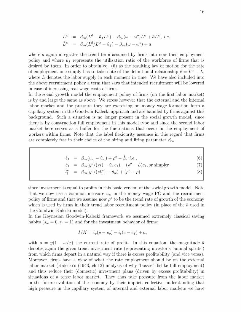
16

Lw = βeu(Ld − ufL

w) − βeω(ω − ωo)Lw + aLw, i.e.

Lw = βeu(Ld/Lw − uf) − βeω(ω − ωo) + a

where a again integrates the trend term assumed by firms into now their employmentpolicy and where uf represents the utilization ratio of the workforce of firms that isdesired by them. In order to obtain eq. (6) as the resulting law of motion for the rateof employment one simply has to take note of the definitional relationship e = Lw − L,where L denotes the labor supply in each moment in time. We have also included intothe above recruitment policy a term that says that intended recruitment will be loweredin case of increasing real wage costs of firms.In the social growth model the employment policy of firms (on the first labor market)is by and large the same as above. We stress however that the external and the internallabor market and the pressure they are exercising on money wage formation form acapillary system in the Goodwin-Kalecki approach and are handled by firms against thisbackground. Such a situation is no longer present in the social growth model, sincethere is by construction full employment in this model type and since the second labormarket here serves as a buffer for the fluctuations that occur in the employment ofworkers within firms. Note that the label flexicurity assumes in this regard that firmsare completely free in their choice of the hiring and firing parameter βeu.

e1 = βeu(uw − uw) + ρo − L, i.e., (6)

e1 = βeu(yp/(xl) − uwe1) + (ρo − L)e1, or simpler (7)

lw1 = βeu(yp/(zlw1 ) − uw) + (ρo − ρ) (8)

since investment is equal to profits in this basic version of the social growth model. Notethat we now use a common measure uw in the money wage PC and the recruitmentpolicy of firms and that we assume now ρo to be the trend rate of growth of the economywhich is used by firms in their trend labor recruitment policy (in place of the a used inthe Goodwin-Kalecki model).In the Keynesian Goodwin-Kalecki framework we assumed extremely classical savinghabits (sw = 0, sc = 1) and for the investment behavior of firms:

I/K = iρ(ρ − ρo) − ie(e − ef ) + a,

with ρ = y(1 − ω/x) the current rate of profit. In this equation, the magnitude adenotes again the given trend investment rate (representing investor’s ’animal spirits’)from which firms depart in a natural way if there is excess profitability (and vice versa).Moreover, firms have a view of what the rate employment should be on the externallabor market (Kalecki’s (1943, ch.12) analysis of why ‘bosses’ dislike full employment)and thus reduce their (domestic) investment plans (driven by excess profitability) insituations of a tense labor market. They thus take pressure from the labor marketin the future evolution of the economy by their implicit collective understanding thathigh pressure in the capillary system of internal and external labor markets we have

17

considered above will lead to conditions in the capital-labor relationship, unwanted byfirms, since persistently high employment rates may give rise to significant changes ofworkforce participation with respect to firms’ decision making, in the hiring and firingdecision of firms, in reductions of the work-day etc., not at all liked by ’industrial leaders’in the case of a Kaleckian dissent economy.In the social growth model, the alternative and extension of this paper to / of a Kaleckianconsent economy, we have already assumed that workers of type II consume their wholeincome (they pay no taxes). With respect to the other type of workers we assume astheir consumption function

C1 = ch1(1 − τh)ω1Ld1, ch propensity to consume, τh tax rate (9)

ω2Lw2h = ch2(1 − τh)ω1L

d1 consumption of household services (10)

Households type I savings is on the basis of our accounting relationships given by

S1 = ω1Ld1 − C1 − ω2L

w2h − ω2(L − (Lw

1 + Lw2f + Lw

2h + Lw2g) − ω2L

r) (11)

due to the assumed solidarity contribution they provide to the second labor market. In-vestment behavior is in the basic form of the social growth model very simple: all profitsof firms are invested and there is no debt or equity financing yet. The growth rate of thecapital stock is thus simply given by K = ρ = Π/K(ρo the steady state rate of profit).On the basis of what we have already assumed we thus get:

K = ρ = yp[1 − ω1(1 + αωαf)/z] − δ, ω2 = αωω1, Lw2f = αfL

d1 (12)

see below with respect to the parameter αf which characterizes the employment policyof firms with respect to the second labor market.For government consumption we finally assume the simple relationship G = γI, i.e.,government consumption per unit of capital grows at the same rate as the capital stock(which allows to integrate fiscal policy with investment behavior in the intensive formof the model).Since the government, workers from the second labor market and pensioners do not saveand since all tax transfers are turned into consumption and the savings of householdsof type I into commodity inventories of firms from which company pensions are to bededucted and since finally all profits are invested it can easily be shown from what waspresented in accounting form in the preceding section that we must have at all times:

Y p + δ1R = C1 + C2 + Cr + I + δK + G, C1 = ch1(1 − τh)ω1Ld1 (13)

18

if firms produce at full capacity Y p = ypK, Ld1 = Y p/z (which they can and will do in

this case). There is thus no demand problem on the market for goods and thus no needto discuss a dynamic multiplier process as in the Goodwin - Kalecki model with whichthis model was compared here. Note that moreover we have by construction of the socialgrowth model at all points in time:

L = Lw1 + Lw

2f + Lw2h + Lw

2g + Lwr = Lw

1 + Lw2 Lr = αrL (14)

We thus assume that households of type 1 must pay as solidarity contribution (employ-ment benefits) those workers of type 2, whose wages are not paid by firms, throughhouseholds type 2 service to households of type I and through the core employment inthe government sector. The government employs in addition as administrative workersand infrastructure workers (public work and education) the remaining workforce in thesecond labor market (plus the Lr services from pensioners). This completes the discus-sion of the behavioral equations of the social growth model, the intensive form of whichwill now be derived in the following section. Compared to the Goodwin-Kalecki modelof Flaschel, Franke and Semmler (2007) this model type will be shown to function veryeasily without need of a discussion of conflict-driven upper and lower turning pointsin economic activity and income distribution which are necessary to keep the locallycentrifugal dynamics of the Goodwin-Kalecki approach bounded and thus viable. Thereare only mildly conflicting income claims in the social growth model and also only mildconflicts about the role and the extent of the welfare state in such a framework (to bediscussed below).In the Goodwin-Kalecki growth cycle model we have (in the dissent situation) conflict-riddled turning points in economic and social activities than can end prosperity phasesin a radical fashion and then lead the society into long-lasting depressions, processesthat are harmful and wasteful with respect to human and physical capital and thatmay not work towards a recovery under all circumstances. The need for an alternativeto such a situation is therefore a compelling one from the perspective of a social anddemocratic society and the potential it may contain for the evolution of mankind. Wehave already introduced in the previous and this section the economic contours of suchan alternative. This alternative model of social reproduction will be analyzed in itsmacrodynamic features in the next two sections.

4 Flexicurity growth: Full capacity convergence to-

wards balanced reproduction

4.1 The dynamics and their balanced growth path

Inserting the equations of the social growth model appropriately into each other givesrise to the following 3D dynamics in the state variables ω1 = w/p, lw1 = Lw

1 /K and

19

l = L/K where the last variable does however not feedback into the first two laws ofmotion due to the construction of the labor markets of the model.9

ω1 = κ[(1 − κp)(βwu(yp

zlw1− uw) − βwω ln(

ω1

ωo1

)) − (1 − κw)βpω ln(ω1

ωo1

)] (15)

lw1 = βeu(yp

zlw1− uw) + n − ρ, ρ = yp[1 − ω1(1 + αωαf)/z] − δ (16)

l = n − (yp[1 − (1 + αωαf )ω1/z] − δ) = yp[(1 + αωαf)(ω1 − ωo1)/z] (17)

However, in order to get a stationary value of l in the long-run we must assume a specialvalue for ωo

1 in the first two equations (as the steady state reference real wage in the firstlabor market), which is determined by:

l = 0, i.e., yp[1 − (1 + αωαf)ω1/z] = δ + n. (18)

The reference wage used in the first two laws of motion must therefore be chosen suchthat the capital stock grows with the natural rate n in the steady state which is one ofthe conditions needed for steady growth in the Harrod (1939) growth model. Since ourmodel is based on Say’s law the other conditions of the Harrod model do not apply here.Based on this assumption we get for the interior steady state or balanced growth pathof the social growth economy the equations (uw = 1 in the following for reasons ofsimplicity):

lwo1 =

yp

uwz=

ldo1

uw

= yp/z (19)

ωo1 =

1 − n+δyp

1 + αfαω

z < z (20)

lo = arbitrary (21)

Since we have a zero determinant for the 3D Jacobian of the above dynamics (since thethird law of motion only depends on the first state variable) we have zero root hysteresisin the 3D system which in the given form allows to treat and solve the first two equationsindependently of the third one which when appended can converge to any value of l,depending on shocks to labor supply, capital formation and the like. Note however thatthis only applies if there is social consensus with respect to the steady state real wageωo

1 as the benchmark for real wage negotiations in the first labor market. Choosing inaddition (and for example) as parameter values10 αw = 0.5, n = 0.05, δ = 0.1, yp = 0.5gives for the ratio v1 = ω1/z, the wage share in the first labor market, the approximate

9The steady state value, see below, is here assumed to underlie Blanchard and Katz (1999) typeerror correction in the first labor market.

10The value of n must be chosen that high since technical change is still ignored in this baseline socialgrowth model.

20

value v1 = 0.64 and for the profit share Πo/Y p the value 0.1 which in sum implies for theshares of wages and government expenditures the value 90%. Note finally that the livingstandards in this society, as measured by real wages, depend of course on the value ofthe labor productivity of workers in the first labor market.

4.2 Monotonic convergence towards balanced growth

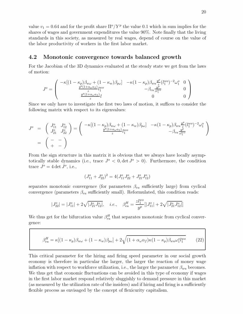
For the Jacobian of the 3D dynamics evaluated at the steady state we get from the lawsof motion:

Jo =

−κ[(1 − κp)βwω + (1 − κw)βpω] −κ(1 − κp)βwuyp

z(lwo

1 )−2ωo1 0

yp(1+αωαf )

zlwo1 −βeu

yp

zlwo1

0yp(1+αωαf )

zl 0 0

Since we only have to investigate the first two laws of motion, it suffices to consider thefollowing matrix with respect to its eigenvalues:

Jo =

(

Jo11 Jo

12

Jo21 Jo

22

)

=

(

−κ[(1 − κp)βwω + (1 − κw)βpω] −κ(1 − κp)βwuyp

z(lwo

1 )−2ωo1

yp(1+αωαf )

zlwo1 −βeu

yp

zlwo1

)

=

(

− −+ −

)

From the sign structure in this matrix it is obvious that we always have locally asymp-totically stable dynamics (i.e., trace Jo < 0, det Jo > 0). Furthermore, the conditiontrace Jo = 4 det Jo, i.e.,

(Jo11 + Jo

22)2 = 4(Jo

11Jo22 + Jo

21Jo12)

separates monotonic convergence (for parameters βeu sufficiently large) from cyclicalconvergence (parameters βeu sufficiently small). Reformulated, this condition reads:

|Jo22| = |Jo

11| + 2√

|Jo21J

o12|, i.e., βH

eu =zlwo

1

yp[|Jo

11| + 2√

|Jo21J

o12|]

We thus get for the bifurcation value βHeu that separates monotonic from cyclical conver-

gence:

βHeu = κ[(1 − κp)βwω + (1 − κw)βpω] + 2

√

(1 + αωαf )κ(1 − κp)βwuωo1l

wo1 (22)

This critical parameter for the hiring and firing speed parameter in our social growtheconomy is therefore in particular the larger, the larger the reaction of money wageinflation with respect to workforce utilization, i.e., the larger the parameter βwu becomes.We thus get that economic fluctuations can be avoided in this type of economy if wagesin the first labor market respond relatively sluggishly to demand pressure in this market(as measured by the utilization rate of the insiders) and if hiring and firing is a sufficientlyflexible process as envisaged by the concept of flexicurity capitalism.

21

4.3 Global viability

For the investigation of global asymptotic stability we will now analyze the core dynam-ical system by means of so-called Liapunov functions. For this purpose we represent the2D dynamics of the preceding section as follows.

ω1 = G1(ω1) + G2(lw1 ), G1′ < 0, G2′ < 0 (23)

lw1 = H1(ω1) + H2(lw1 ), H1′ > 0, H2′ < 0 (24)

The Liapunov function to be used in the stability proof then reads as follows:

V (ω1, lw1 ) =

∫ ω1

ωo1

H1(ω1)/ω1dω1 +

∫ lw1

lwo1

−G2(lw1 )/lw1 dlw1

This function describes by its graph a 3D sink with the steady state of the economy as itslowest point, since the above integrates two functions that are negative to the left of thesteady state values and positive to their right. For the first derivative of the Liapunovfunction along the trajectories of the considered dynamical system we moreover get:

V = dV (ω1(t), lw1 (t))/dt =

(

H1(ω1)/ω1

)

ω1 −(

G2(lw1 )/lw1)

lw1 (25)

= H1(ω1)ω1 − G2(lw1 )lw1 (26)

= H1(ω1)(G1(ω1) + G2(lw1 )) − G2(lw1 )(H1(ω1) + H2(lw1 )) (27)

= H1(ω1)G1(ω1) − G2(lw1 )H2(lw1 ) (28)

= −H1(ω1)(−G1(ω1)) − (−G2(lw1 ))(−H2(lw1 )) (29)

≤ 0 [= 0 if and only if ω1 = ωo1, l

w1 = lwo

1 ] (30)

since the multiplied functions have the same sign to the right and to the left of theirsteady state values and thus lead to positive products with a minus sign in front ofthem (up to the situation where the economy is already sitting in the steady state). Wethus have proved that there holds:

Proposition 1:

The interior steady state of the dynamics

ω1 = κ[(1 − κp)(βwu(yp

zlw1− uw) − βwω ln(

ω1

ωo1

)) − (1 − κw)βpω ln(ω1

ωo1

)] (31)

lw1 = βeu(yp

zlw1− uw) + ρo + (yp[(ω1 − ωo

1)(1 + αωαf )/z] − δ) (32)

is a global sink of the function V, defined on the positive orthant of the phase

space, and is attracting in this domain, since the function V is strictly de-

creasing along the trajectories of the dynamics in the positive orthant of the

phase space.

22

From the global perspective there may however be supply bottlenecks in the secondlabor market. Here we assume that the economy is working always in a corridor aroundthe steady state where the government as the employer of first resort has still a sufficientamount of workforce working in the range of activities that is organized by it. Due tothe stability results obtained in the present and the preceding section this is not a veryrestrictive assumption under the normal working of the economy.

5 Company pension funds: Dynamics and steady

state levels

There is a further law of motion in the background of the model that needs to beconsidered in order to provide an additional statement on the viability of the consideredmodel of flexicurity capitalism. This law of motion describes the evolution of the pensionfund per unit of the capital stock η = R

Kand is obtained from the defining equation

R = S1 − δ1R as follows:

η = R − K =R

K

K

R− ρ =

S1 − δ1R

K/η − ρ, i.e. :

η =S1

K− (δ1 + ρ)η = s1 − (δ1 + ρ)η

with savings of households of type I and profits of firms per unit of capital being givenby:

s1 = (1 − (ch1 + ch2)(1 − τh) − τh)ω1yp/z − αωω1(l

wx + lr)

lwx = l − (lw1 + lw2f + lw2h + lw2g)

lr = αrl, i.e., due to the financing of the employment terms lw2h + lw2g

s1 = (1 − ch1(1 − τh) − αgτh)ω1yp/z − ((1 + αr)l − (lw1 + lw2f ))αωω1, lw2f = αfy

p/z

ρ = yp[1 − (1 + αωαf)ω1/z] − δ

For reasons of analytical simplicity we now assume that the government pursues animmigration policy that ensures for the total growth rate of the labor force the conditionn = K, i.e., the total labor supply grows by this migration policy with the same rate asthe capital stock. This keeps the ratio l = L/K constant, a simplifying assumption thatmust be accompanied later on by the assumption that the actual l must be chosen in acertain neighborhood of a base value lo that is determined later on. Since we are now nolonger able to determine the steady state value of the real wage ω1 from the law of motionfor l, we have to supply it from the outside now: ωo

1 = ω1 = given. This also providesus with the steady state value of the rate of profit ρo = ρ = yp[1 − (1 + αωαf)ω1/z] − δwhich also determines the steady value of natural growth no = ρ. Moreover we alsoassume for simplicity δ1 = δ for the depreciation rates of the capital stock and the stockof pension funds.This gives for the law of motion of the pension fund to capital ratio the differentialequation:

23

η = (1 − ch1(1 − τh) − αgτh)ω1yp/z − ((1 + αr)l − (lw1 + αfy

p/z))αωω1

−[yp − (1 + αωαf)ω1yp/z]η

We thus get that the trajectory of the pension fund ratio η is driven by the autonomousevolution of the state variables ω1, l

w1 that characterize the dynamics of the private sector

of the economy and that has been shown to be convergent to the steady state valuesω1, l

wo1 = yp/z as usual). Assuming that these variables have reached their steady state

positions then gives

η = (1 − ch1(1 − τh) − αgτh)ω1yp/z − ((1 + αr)l − (lwo

1 + αfyp/z))αωω1 − (δ1 + ρ)η

which gives a single linear differential equation for the ratio η. This dynamic is globallyasymptotically stable around its steady state position (lwo

1 = yp/z):

ηo =(1 − ch1(1 − τh) − αgτh)ω1y

p/z − ((1 + αr)l − (1 + αf)yp/z)αωω1

δ1 + ρ

In this simple case we thus have monotonic adjustment of the pension-fund capital ratioto its steady state position, while in general we have a non-autonomous adjustment ofthis ratio that is driven by the real wage and employment dynamics of the first labormarket. the steady state level of η is positive iff there holds for the full employmentlabor intensity ratio:

l <(1 − ch1(1 − τh) − αgτh)ω1y

p/z + ((1 + αf)yp/z)αωω1

(δ1 + ρ)(1 + αr)αωω1

We now assume moreover that the additional company pension payments to pensionersshould add the percentage 100αc to their base pension ω2αr l per unit of capital. Wethus have as further restriction on the steady state position of the economy, if there isan αc target given, namely:

δ1ηo = αcωo2αr l, ωo

2 = αωω1

Inserting the value for ηo then gives

αc = δ1(1 − ch1(1 − τh) − αgτh)ω1y

p/z − ((1 + αr)l − (1 + αf )yp/z)αωω1

(δ1 + ρ)ωo2αr l

We thus get that a target value for αc demands a certain labor intensity ratio l andvice versa. For a given total labor intensity ratio there is a given percentage by whichcompany pensions compare to base pension payments. This percentage is the larger thesmaller the ratio lwo

1 /l due to the following reformulation of the αc formula:

αc = δ1[(1 − ch1(1 − τh) − αgτh)ω1 + (1 + αf)αωω1]l

wo1 /l − (1 + αr)αωω1

(δ1 + ρ)αrαωω1(33)

24

If this value of the total employment labor intensity ratio prevails in the consideredeconomy (where it is of course as usually assumed that ch1(1 − τh) + αgτh < 1 holds)we have that core pension payments to pensioners are augmented by company pensionpayments by a percentage that is given by the parameter αc and that these extra pensionpayments are distributed to pensioners in proportion to their contribution to the timethat they have worked in the private sector of the economy. There is thus a negativetrade-off between the ratios l, αc, as expressed by the relationship (33). It also shows thatthe total working population must have a certain ratio to the capital stock in order toallow for a given percentage of extra company pension payments.: Due to δ1ηo = αcω

o2αr l

and so1 = (δ1 + ρ)ηo we also have the equivalence between positive savings per unit of

capital of households of type I and positive values for αc, ηo. Moreover, these values arein fact positive if there holds:11

l <(1 − ch1(1 − τh) − αgτh)ω1y

p/z + (1 + αf)yp/z)αωω1

(δ1 + ρ)(1 + αr)αωω1

This inequality set limits to the total labor-supply capital-stock ratio l which allows forpositive savings of households of type I in the steady state and thus for extra pensionpayments to them later on. Households of type I are by and large financing the secondlabor market through taxes and employment benefits (besides their contribution to thebase income of the retired people). Since firms have a positive rate of profit in the steadystate, since the government budget is always balanced and since only households of typeI save in this economy, we have thus now established the condition under which suchan economy accumulates not only capital, but also pensions funds – under appropriaterestrictions on labor supply – to a sufficient degree.

6 Pension funds and credit

In this section we will investigate the implications of the situation where pension fundsare used for real capital formation instead of remaining idle except of being used forcompany pension payments (of amount δ1R at each point in time). The productive useof part of the pension fund R is here assumed to be rewarded at the constant interestrate r applied to the debt level D accumulated by the firms in the private sector of theeconomy.

6.1 Accounting relationships

Pension funds as quasi commercial banks who give credit to firms out of their funds andthus allow firms to invest in good times much beyond their retained earnings, i.e., profitsnet of interest payments on loans.

11Note that the numerator is easily shown to be not only positive, but even larger than 1 understandard Keynesian assumptions on expenditure and taxation rates.

25

Firms

Production and Income Account:Uses Resources

δK δKω1L

d1 = ω1Y

p/z C1 + C2 + Cr

ω2Lw2f = αωω1αfY

p/z GrDΠ I = (iρ(ρ − ρo) − id(d − do) + a)KY p Y p

We denote by ρn the profit rate that would prevail at normal rates of capacity utilization,while the capacity utilization effect on investment is captured by the first term in theinvestment function. Animal spirits are here represented by the exogenously given terma which may be subject to sudden shifts, representing golden periods or leaden ages.respectively. We assume that enough credit is generally available to support suddenupward shifts in trend investment. The financing of gross investment is shown in thenext account.

Investment and Credit:Uses Resources

δK δKI = (iρ(ρ − ρo) − id(d − do) + a)K Π

D = I − ΠIg Ig

We assume as investment behavior of firms the functional relationship:

I/K = iρ(ρ − ρo) − id(d − do) + a.

This investment schedule states that investment plans depend positively on the deviationof the profit rate from its steady state level and negatively on the deviation of the debtto capital ratio from its steady state value. The exogenous trend term in investmentis a and it is again assumed that it represents the influence of investing firms ‘animalspirits’ on their investment activities.

Firms Net Worth:Assets Liabilities

K DReal Net Worth

K K

In the management of pension funds we assume that a portion sR of them is held asminimum reserves and that a larger portion of them has been given as credit D to firms.The remaining amount are idle reserves Ds, not yet allocated to any interest bearingactivity.

26

Pension Funds

Pension Funds and Credit (stocks):Assets Liabilities

R sRDX excess reserves

R R

Pension funds receive the Savings of households of type 1 (the other households do notsave) and they receiver the interest payments of firms. They allocate this into requiredreserve increases, payments to pensioners, new credit demand of firms and the rest asan addition or substraction to their idle reserves.

Pension Funds and Credit (flows):Resources Uses

S1 sRrD δ1R + rD

D = I − Π

XS1 + rD S1 + rD

The above representation of the flows of funds in the pension funds system implies forthe time derivative of accumulated funds R the relationship

R = S1 − δ1R − (I − Π) = S1 + Π − δ1R − I, i.e.,

it is given by the excess of savings of households of type I over current company pensionfunds payments to retired households and the new credit that is given to firms to financethe excess of investment over retained profits.

Households I and II (primary and secondary labor market)

Income Account (Households I):Uses Resources

C1 = ch1(1 − τh)Yw1

ω2Lw2h = ch2(1 − τh)Y

w1

T = τhYw1

ω2(L − (Lw1 + Lw

2f + Lw2h + Lw

2g))ω2L

r

S1 ω1Ld1

Y w1 Y w

1

Households in the first labor market consume with a constant marginal propensity outof the income after primary taxes and they employ households services in constant

27

proportions to the consumption habits. They pay the wages of the workers in thesecond labor market that are not employed by firms, by them and the government as aquasi unemployment benefit insurance (a generational solidarity contribution) and theypay the common base rent of all pensioners (as intergenerational contribution). Theremainder represents their contribution the pension scheme of the economy, from whichthey will receive δ1R+rD when retired. We consider this as a possible scheme of fundingthe excess employment and the pensioners, not necessarily a just one however.

Income Account Households IIUses Resources

C2 ω2Lw2

Y w2 Y w

2

Income Account (Retired Households):Uses Resources

Cr ω2Lr + δ1R + rD

Y r Y r

The Government

Income Account – Fiscal Authority / Employer of First Resort:Uses Resources

G = αgτhYw1 T = τhY

w1

ω2Lw2g = (1 − αg)τhY

w1

ω2Lwx ω2(L − (Lw

1 + Lw2f + Lw

2h + Lw2g))

ω2Lr ω2L

r

Y g Y g

Government gets primary taxes and spends them on goods as well as services in thegovernment sector (which are here determined residually). It administrates the commonbase rent payments as well as the payments of those not yet employed in the sectorsof the economy. Its workforce consists of all workers that are not employed by firmsof households of type 1 and also of all pensioners that are still capable to work. Themodel therefore assumes not only that there is a work guarantee for all, but also a workobligation for all members in the workforce, with the addition of those that are retiredbut still able and willing to work.

6.2 Investment and credit dynamics in flexicurity growth

For simplicity we here again assume that the government pursues an immigration policythat ensures for the growth rate of the labor force the condition n = K, i.e., the totallabor supply grows by this migration policy with the same rate as the capital stock.

28

This again keeps the ratio l = L/K = l = constant. Since we are again no longer ableto determine the steady state value of the real wage ω1 from the law of motion for l,we have to supply it again from the outside: ωo

1 = ω1 = given. This however no longeralso provides us with the steady state value of the rate of profit, since profits are nowto be determined net of interest payments: ρ = yp[1− (1 + αωαf )ω1/z]− δ1 − rd, whered = D/K denotes the indebtedness of firms per unit of capital. We assume again astrend term in Okun’s law the growth rate of the capital stock (i.e., this part of the newhiring is just determined by the installation of new machines or whole plants (underthe assumption of fixed proportions in production). The normal level of the rate ofemployment of the workforce employed by firms is again set equal to ‘1’ for simplicity.On the basis of these assumptions we get from what was formulated in the precedingsubsection (where investment was assumed to be given now by I/K = iρ(ρ−ρo)− id(d−do) + a):

lw1 = βeu(yp

zlw1− 1)

ω1 = κ[(1 − κp)(βwu(yp

zlw1− 1) − βwω ln(

ω1

ω1)) − (1 − κw)βpω ln(

ω1

ω1)]

d = [iρ(ρ − ρo) − id(d − do) + a](1 − d) − ρ

η = s1 + ρ − (δ1η + (1 + η)[iρ(ρ − ρo) − id(d − do) + a])

= (1 − ch1(1 − τh) − αgτh)ω1yp/z − ((1 + αr)l − (lw1 + αfy

p/z))αωω1

+ [yp[1 − (1 + αωαf)ω1/z] − δ1 − rd] − (δ1η + (1 + η)[iρ(ρ − ρo) − id(d − do) + a])

The introduction of debt financing of firms thus makes the model considerably moreadvanced in its economic structure, but not so much from the mathematical point ofview, due to the recursive structure that characterizes the dynamical system at this levelof generality. We note that there is not yet an interest rate policy rule involved in thesedynamics, but the assumption of an interest rate peg: r = const.We make use in the following of the following abbreviations:

so1 = (1 − ch1(1 − τh) − αgτh)ω1y

p/z − ((1 + αr)l − yp/z(1 + +αf))αωω1

andρmax = yp[1 − (1 + αωαf )ω1/z] − δ1.

On the basis of such steady state expressions we then have:

Proposition 2:

The interior steady state of the considered dynamics is given by:12

lwo1 =

yp

z, ωo

1 = ω1, ηo =so1 + ρo − a

δ1 + a,

where do, ρo have to be determined by solving the two equations

ρo = ρmax − rdo, ρo = a(1 − do)

12The steady state value of so

1is the same as in the preceding section.

29

which gives for the steady state values of d, ρ, η the expressions:

do =a − ρmax

a − r, ρo = a

ρmax − r

a − r, ηo =

so1 + aρmax−r

a−r

δ1 + a=

so1(a − r) − a(a − ρmax)

(δ1 + a)(a − r).

We assume that both the numerator and the denominator of the fraction that definesdo are positive, i.e., the trend term in investment is sufficiently strong (larger than therate of profit before interest rate payments ρmax and larger than the rate of interest r).Moreover, it is also assumed that ρmax > r holds so that all fractions shown above arein fact positive. In the case where a = ρmax = yp[1 − (1 + αωαf)ω1/z] − δ1 holds wehave do = 0 and ρo = a in which case the value of ηo is the same as in the sections oninvestment without debt financing. Nevertheless the dynamics around the steady stateremain debt financed and are therefore different from the one of the preceding section.We thus can have a ‘balanced budget’ of firms in the steady state while investmentremains driven by I/K = iρ(ρ − ρo) − id(d − do) + a outside the steady state position.For the fraction of company pension funds divided by base pension payments we nowget as relationship in the steady state

αc =δ1ηo + rdo

αωαrω1l

an expression that in general does not give rise to unambiguous results concerning com-parative dynamics. In the special case do = 0 we however can state that this fractiondepends positively on s1

o (also in general) and negatively on a, δ1, l.The Jacobian at the interior steady state of the here considered 4D dynamics reads

Jo =

−βeu/lwo1 0 0 0

? −κ[(1 − κp)βwω + (1 − κw)βpω] 0 0? ? −(iρ + id)(1 − do)) − (a − r) 0? ? ? −a(1 + δ1)

This lower triangular form of the Jacobian immediately implies that the elements onthe diagonal of the matrix Jo are just equal to the 4 eigenvalues of this matrix whichare therefore all real and negative. This gives:

Proposition 3:

The interior steady state of the considered dynamics is locally asymptotically

stable and is characterized by a strict hierarchy in the state variables of the

dynamics.

Due to the specific form of the considered laws of motion we conjecture that the steadystate is also a global attractor in the economically relevant part of the 4D phase space.We then would get again monotonically convergent trajectories from any starting pointof this part of the phase space and thus fairly simple adjustment processes also in thecase where investment is jointly financed by profits (retained earnings) and credit.The stability of the steady state is increased (i.e., the eigenvalues of its Jacobian ma-trix become more negative) if the speed parameter characterizing hiring and firing is

30

increased, if Blanchard / Katz type error correction becomes more pronounced and ifthe parameters iρ, id, a in the investment function are increased.Summing up, we thus can state that the adjustment processes and their stability prop-erties remain very supportive for the working of our model of flexicurity type which isgenerally monotonically convergent with full capacity utilization of both capital and la-bor to a steady state position with a sustainable distribution of income between firms, ourthree types of households and the government. We conclude that flexicurity capitalismmay be a workable alternative to current forms of capitalism and can avoid in particularthe severe social deformations and the human degradation caused by the reserve armymechanism and the mass unemployment it implies for certain stages in a long-phasedistributive and welfare state cycle, in the US and the UK more of a neoclassical coldturkey type and in Germany and in France more gradualistic in nature.13

7 Outlook: Keynesian demand problems

As an outlook we here briefly sketch a situation where capacity utilization problemsas well as stability problems may arise within the flexicurity variant of a capitalisticeconomy. We modify the baseline model of section 2 in a minimal way in order toobtain such results. In place of pension funds as well as the credits they give to firmswe now consider the situation where firms finance their investment plans through theirprofits and through the issuing of corporate bonds. We assume these bonds to be of thefixprice variety and we also keep the rate of interest that is paid on these bonds fixedfor simplicity.The amount of such bonds that firms have issued in the past is denoted by B and theirprice is 1 in nominal units. Firms thus have to pay rB as interest at the current point intime and they intend to use their real profits net of interest rate payments and in additionthe issue Bs/p to finance their rate of investment I/K = iρ(ρ−ρo)− ib(

BpK

− ( BpK

)o)+ a.This rate of investment is assumed to depend positively on excess profitability comparedto the steady state rate of profit and negatively the deviation of their debt from its steadystate level.

Firms

Production and Income Account:Uses Resources

δK δKω1L

d1, L

d1 = Y/z C1 + C2 + Cr

ω2Lw2f , ω2 = αωω1, L

w2f = αfL

d1 G

rB/p I = iρ(ρ − ρo)K − ib(Bp− (B

p)o) + aK

Π(= Y f) [I = Π + Bs/p]Y Y

13We refer the reader back to what is shown in figure 3 where the postwar period up into the 1960’sseemed to suggest that the working of the reserve army mechanism had been overcome, a suggestionthat was disproved in the subsequent years in a striking way.

31

Households of type I behave as was assumed so far, but attempt to channel their realsavings now into corporate bond holdings as shown below. They will be able to exactlysatisfy their demand for new bonds when there is goods market equilibrium prevailing(I = S), since only firms and these households act on this market, while all othereconomic units just spend what they get (with balanced transfer payments organizedby the government). The real return from savings in corporate bonds rB/p, at eachmoment in time, will be added below to the base rent payments of retired households,who receive these benefits in proportion to the bonds they have allocated during theirworklife in the private sector of the economy. The bonds allocated in this way thusonly generate a return when their holders are retired and then – as in the pension fundscheme of section 2 – at the then prevailing market rate of interest (which is here agiven rate still). The pension fund model is therefore here only reformulated in terms ofnominal paper holdings (coupons) and thus no longer based on the storage of physicalmagnitudes. Hence, corporate bonds are here not only of a fix-price variety, but alsoprovide their return only after retirement. This is shown in the income account ofretired persons below. The income account of the workers in the second labor market isunchanged and therefore not shown here again.

Households I (primary labor market) and Retired Households

Income Account (Households I):Uses Resources

C1 = ch1(1 − τh)ω1Ld1

ω2Lw2h = ch2(1 − τh)ω1L

d1

T = τhω1Ld1

ω2(L − (Lw1 + Lw

2f + Lw2h + Lw

2g))ω2L

r, Lr = αrL

S1[= Bd/p] ω1Ld1

Y w1 = ω1L

d1 Y w

1 = ω1Ld1

Income Account (Retired Households):Uses Resources

Cr ω2Lr + rB/p, Lr = αrL

Y r Y r

The government income account (not shown) is also kept unchanged and in particularbalanced in the way used in the preceding model types. The modifications of the modelof section 2 are therefore of a minimal kind, largely concerning a different type of in-vestment behavior of firms and a new type of organizing the formerly assumed companypension funds. However, the assumed flexicurity system becomes now of real impor-tance, since we here will get demand determined (Keynesian) business cycle fluctuationsin the dynamics implied by the model, whereas firms did not face capacity under- or

32

over-utilization problems in the earlier model types. Keynesian IS-equilibrium determi-nation has to be considered now and gives rise to the following equation for the effectiveoutput per unit of capital (characterizing goods market equilibrium):14

Y/K = y = C1/K + C2/K + Cr/K + δ + I/K + G/K

= ch(1 − τh)ω1y

z+ αωω1(l − lw1 ) + αωαrω1l + rb

+δ + iρ(ρ − ρo) − ib(b − bo) + a + αgτhω1y/z

ρ = y − (1 + αfαω)ω1y/z − δ − rb, b = B/(pK)

which taken together gives:

y =αωω1(l − lw1 ) + αωαrω1l + (rb + δ)(1 − iρ) − iρρo − ib(b − bo) + a

1 − [ch(1 − τh) + αgτh − iρ(1 + αfαω)]ω1/z − iρ= y(lw1 , ω1, b, . . . )

Note that we have modified the investment function in this section to i(·) = iρ(ρ−ρo)−ib(b − bo) + a. Note also that we have again assumed that natural growth n is alwaysadjusted to the growth rate of the capital stock K. We also assume that the denominatorin the above fraction is positive and now get the important result that output per unitof capital is no longer equal to its potential value, but now depending on the marginalpropensity to spend as well as on other parameters of the model. This is due to the newsituation that firms use corporate bonds to finance their excess investment (exceedingtheir profits) or buy back such bonds in the opposite case and that households of type Ibuy such bonds from their savings (and thus do not buy goods in this amount anymore toincrease the pension fund). We thus have independent real investment and real savingsdecisions which – when coordinated by the achievement of goods market equilibriumas shown above – lead to a supply of new corporate bonds that is exactly equal to thedemand for such bonds at this level of output and income. This simply follows fromthe fact that only firms and households of type I are saving, while all other budgets arebalanced. Households of type I thus just have to accept the amount of the fixed pricebonds offered by firms and are thereby accumulating these bonds (whose interest ratepayments are paid out to retired people according to the percentage they have achievedwhen retiring).Assuming the accumulation of corporate bonds in the place of real commodities andan investment function that is independent from these savings conditions thus impliesthat the economy is subject to Keynesian demand rationing processes (at least closeto its steady state). These demand problems are here derived on the assumption ofIS-equilibrium and thus represented in static terms in place of a dynamic multiplierapproach that can also be augmented further by means of Metzlerian inventory adjust-ment processes. We stress once again that the possibility for full capacity output is hereprevented through the Keynesian type of underconsumption assumed as characterizingthe household type I sector and the fact that there is then only one income level thatallows savings in bonds to become equal to bond financed investment in this simplecredit market that is characterizing this modification of the flexicurity model, due to thenow existing effective demand schedule y(lw1 , ω1, b, . . . ). We assume that the parametersare chosen such that we get for the partial derivatives of the effective demand function

14Standard Keynesian assumptions will again ensure that yo > 0 holds true.

33

y :ylw

1(lw1 , ω1, b, . . . ) < 0, yω1

(lw1 , ω1, b, . . . ) > 0, yb(lw1 , ω1, b, . . . ) < 0

holds true. This is fulfilled for example if the expression in the denominator of the ef-fective demand function is negative and if the parameter ib is chosen sufficiently large.Effective demand is then wage led and flexible wages therefore dangerous for the con-sidered economy.As now significantly interacting laws of motion we have in the consider case:

lw1 = βeu(y

zlw1− 1)

ω1 = κ[(1 − κp)(βwu(y

zlw1− 1) − βwω ln(

ω1

ωo1

)) − (1 − κw)(βpu(y

yp− uc) + βpω ln(

ω1

ωo1

))]

b = (1 − b)(iρ(ρ − ρo) − ib(b − bo) + a) − ρ − pb

p = κ[βpy(y

yp− uc) + βpω ln(

ω1

ωo1

+ κp(βwu(y

zlw1− 1) − βwω ln(

ω1

ωo1

)] + πc

πc = βπcp(0 − πc)

where p has to be inserted into the other equation (where necessary) in order to arrive atan autonomous system of 4 ordinary differential equations. This particular formulationof the debt financing of firms thus makes the model considerably more advanced fromthe mathematical as well as from an economic point of view. We note that there is notyet an interest rate policy rule involved in these dynamics, but that the assumption ofan interest rate peg is maintained still: r = const.The laws of motion describe again (in this order) our formulation of Okun’s law, the realwage dynamics as it applies in a Keynesian environment (see section 3), the debt dy-namics of firms and a simple regressive expectations scheme concerning the inflationaryclimate surrounding the wage-price spiral where it is assumed (and in fact also takingplace) that inflation converges back to a constant price level. There is therefore notyet an inflation accelerator present in the formulation of the dynamics of the four statevariables of the model. Nevertheless, price level inflation is now explicitly taken accountof, indeed for the first time in this paper.Steady state and stability analysis is no longer straightforward in this Keynesian variantof flexicurity capitalism. With respect to steady state positions we have to solve nowa simultaneous equation system in the variables ω1, ρ, b. Due to the structure of theeffective demand function we have moreover no longer zero entries in the Jacobian ofthe dynamics at the steady state of the first three state variables (the last law of motionis a completely trivial one). As economic mechanism we can identify a real wage channelas in the Kaleckian dynamics (working here in a wage led environment by assumption).There is furthermore the dynamic of the debt to capital ratio of firms. these feedbackchannels can be tamed through appropriate assumptions, but are even then working inan environment that gives no straightforward economically plausible stability assertions,due to the strong interactions present in the dynamics. We therefore have to leave thestability analysis for future research here.The conclusion of this section therefore is that effective demand problems can make flex-icurity capitalism significantly more difficult to analyze and therefore demand a treat-ment of much more depth – including inflation and interest rate policy rules, government

34

deficits and fiscal policy rules, etc. – than was possible in this concluding section. More-over, credit relationships may be looked for that avoid the increase in complexity of thedynamics of this concluding section.

35

References

Blanchard, O.J. and L. Katz (1999): Wage dynamics: Reconciling theory andevidence. American Economic Review. Papers and Proceedings, 69 – 74.

Bronfenbrenner, M. (1969): Is the Business Cycle Obsolete? New York: Wiley.

Desai, M. (1984): An econometric model of the share of wages in national income:UK 1855 – 1965. In: R.M. Goodwin et al. (eds.): Nonlinear Models of Fluctuating

Growth. Heidelberg: Springer, 253 – 277.

Flaschel, P. (1984): Some stability properties of Goodwin’s growth cycle model.Zeitschrift fur Nationalokonomie, 44, 63-69.

Flaschel, P., Franke, R. and W. Semmler (2007): Kaleckian Investment andEmployment Cyclesin Postwar Industrialized Economies. Scepa, New School University, New York:Working paper.

Flaschel, P. and G. Groh (1995): The Classical growth cycle: Reformulation,simulation and some facts. Economic Notes, 24, 1995, 293 – 326.

Flaschel, P. and H.-M. Krolzig (2006): Wage-price Phillips curves and macroeco-nomic stability: Basic structural form, estimation and analysis. In: C. Chiarella, P.Flaschel, R. Franke and W. Semmler (eds.): Quantitative and Empirical Analysis

of Nonlinear Dynamic Macromodels. Contributions to Economic Analysis (SeriesEditors: B. Baltagi, E. Sadka and D. Wildasin). Elsevier, Amsterdam.

Flaschel, P., Tavani, D., Taylor, L. and T. Teuber (2007): A structuralistmodel of the wage-price spiral with non-linear demand pressure terms. Scepa,New School University, New York: Working paper, forthcoming.

Goodwin, R. (1967): A growth cycle. In: C.H. Feinstein (ed.): Socialism, Capitalism

and Economic Growth. Cambridge: Cambridge University Press, 54 – 58.

Groth, C. and J. B. Madsen (2007): Medium-term fluctuations and the ”GreatRatios” of economic growth. Copenhagen: mimeo.

Harrod, R. (1939): An essay in dynamic economic theory. The Economic Journal

XLIX, 14-33.

Kalecki, M. (1943): Political aspects of full employment. Reprinted in M. Kalecki,Selected Essays on the Dynamics of the Capitalist Economy, Cambridge: Cam-bridge University Press, 1971.

Kauermann, G., Teuber, T. and P. Flaschel (2007): Exploring US BusinessCycles with Bivariate Loops using Penalized Spline Regression. CEM Bielefeld:working paper.

Solow, R. (1956): A contribution to the theory of economic growth. Quarterly Jour-

nal of Economics, 70, 65-94.