various ways of representing surfaces and basic examples

Chapter 1

Various Ways ofRepresenting Surfacesand Basic Examples

Lecture 1.

a. First examples. For many people, one of the most basic imagesof a surface is the surface of the Earth. Although it looks flat tothe naked eye (at least in the absence of any striking geographicfeatures), we learn early in our lives that it is in fact round, and thatits shape is very well approximated by a sphere. Geometrically, thesphere is defined as the locus of points at a fixed distance, called theradius, from a given point, the centre. Using Cartesian coordinatesand putting the origin at the centre, we derive the familiar equation

(1.1) x2 + y2 + z2 = R2,

where R is the radius; the sphere is the set of all points in R3 whosecoordinates (x, y, z) satisfy this equation.

Many other familiar shapes can also be defined geometrically andrepresented as the set of solutions of a single equation, as in (1.1). Forexample, the (round) cylinder is the locus of points at a fixed distancefrom a given straight line. If the line is taken to be the z-axis and the

1

2 1. Various Ways of Representing Surfaces and Examples

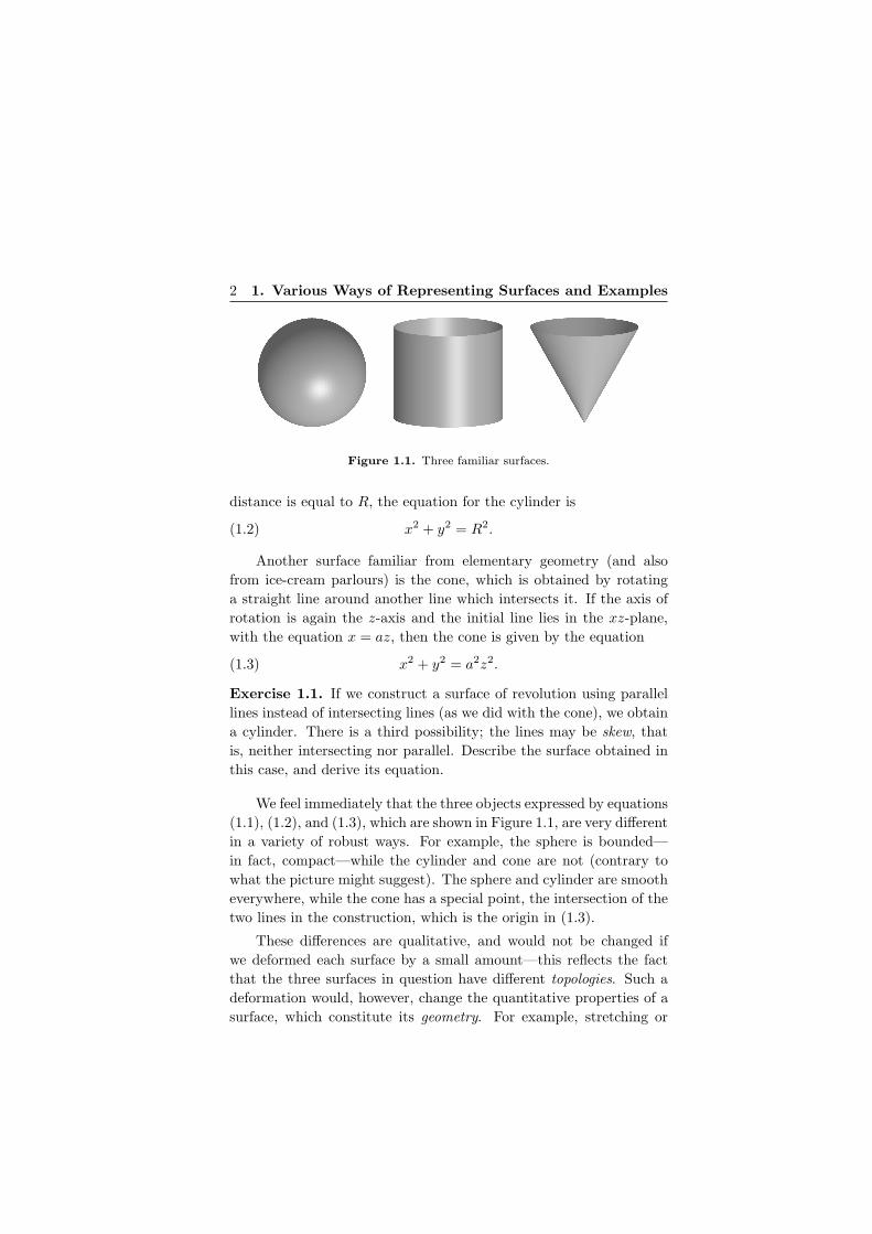
Figure 1.1. Three familiar surfaces.

distance is equal to R, the equation for the cylinder is

(1.2) x2 + y2 = R2.

Another surface familiar from elementary geometry (and alsofrom ice-cream parlours) is the cone, which is obtained by rotatinga straight line around another line which intersects it. If the axis ofrotation is again the z-axis and the initial line lies in the xz-plane,with the equation x = az, then the cone is given by the equation

(1.3) x2 + y2 = a2z2.

Exercise 1.1. If we construct a surface of revolution using parallellines instead of intersecting lines (as we did with the cone), we obtaina cylinder. There is a third possibility; the lines may be skew, thatis, neither intersecting nor parallel. Describe the surface obtained inthis case, and derive its equation.

We feel immediately that the three objects expressed by equations(1.1), (1.2), and (1.3), which are shown in Figure 1.1, are very di!erentin a variety of robust ways. For example, the sphere is bounded—in fact, compact—while the cylinder and cone are not (contrary towhat the picture might suggest). The sphere and cylinder are smootheverywhere, while the cone has a special point, the intersection of thetwo lines in the construction, which is the origin in (1.3).

These di!erences are qualitative, and would not be changed ifwe deformed each surface by a small amount—this reflects the factthat the three surfaces in question have di!erent topologies. Such adeformation would, however, change the quantitative properties of asurface, which constitute its geometry. For example, stretching or

Lecture 1. 3

Figure 1.2. Three ellipsoids.

squeezing the sphere along the three coordinate axes produces anellipsoid given by the equation

(1.4)x2

a2+

y2

b2+

z2

c2= 1,

where a, b, and c are parameters which depend on the degree ofstretching or squeezing. Of the three surfaces above, the overall shapeand crude properties of an ellipsoid (its topology) are most similarto that of a sphere, and are quite di!erent from that of a cylinderor a cone; its geometry, however, displays many di!erences from thegeometry of a sphere.1 For example, the sphere has many symmetries(that is, rigid motions of the space which leave the sphere as a wholein place), while a triaxial ellipsoid (one for which all three numbersa, b, and c in (1.4) are di!erent, such as the third shape shown inFigure 1.2) has only a few.

Exercise 1.2. Find all the symmetries for

(1) a triaxial ellipsoid;

(2) an ellipsoid of revolution for which a = b != c (such as thesecond ellipsoid in Figure 1.2).

Consider separately the symmetries which can be e!ected by a contin-uous motion of the space and those which cannot, such as reflectionswith respect to planes.

1For the time being, we rely on intuitive ideas of what constitutes a general shape.For a reader steeped in mathematical rigor, we refer to notions of homeomorphism anddi!eomorphism, which will be introduced later in Lectures 4 and 17, respectively, andsay that two surfaces have similar shapes if they are homeomorphic, or di!eomorphicin the case of smooth surfaces.


Figure 1.3. A torus and a handle.

Another familiar example of a surface is a torus—just as thesphere is the surface of a idealised ball, the torus is the surface ofan idealised doughnut (or perhaps a bagel, depending on what sortof diet one is on). Like our first three examples, it is a surface ofrevolution, and may be obtained by rotating a circle around a linewhich lies in the plane of the circle, but does not intersect it. We willderive a nice equation (1.5) for the torus in the next lecture.

We can obtain new surfaces with qualitatively distinctive shapesby the procedure called “attaching a handle”. A handle can bethought of as a torus with a hole (or if you like, an inner tube witha small patch cut out), as shown in Figure 1.3—this is attached toa hole cut in a given surface. Applying this procedure to a sphereproduces a surface in the general shape of a torus. If we continue toattach more handles, we obtain something reminiscent of a pretzelwith an increasing number of holes or, alternatively, a chain of torilinked to each other—Figure 1.4 shows a sphere with two handles.Like all the surfaces we have dealt with so far, these surfaces canalso be represented by equations with a certain amount of e!ort (seeExercise 1.6).

b. Equations vs. other methods. We have obtained several dif-ferent surfaces as the set of points whose coordinates (x, y, z) satisfyone equation or another. It is natural to ask what sort of equationswill always yield nice, recognisable surfaces. Will any old equationdo? Or must we impose some restrictions? And conversely, can werepresent every surface by an equation?

Lecture 1. 5

Figure 1.4. A sphere with two handles.

We begin by asking what sorts of equations are acceptable. Bymoving all the terms to the same side, any equation in x, y, and z canbe written in the form F (x, y, z) = 0. If we hope to get a smooth sur-face, we must demand that the function F is at least di!erentiable—any of the equations (1.1), (1.2), (1.3), and (1.4) can be written inthis form with a quadratic polynomial as the function F . But whyare the sphere, the cylinder, and the ellipsoid all smooth, while thecone has a special point? The di!erence is clearly seen in the geo-metric description of the surfaces, since the line we use to define thecone passes through the axis of rotation, but it is not so easy to seewhat feature of the equations is responsible. How does this point ofnon-smoothness turn up in the equations?

The answer is that the origin is a critical point of the functionx2 +y2"a2z2 and lies on the surface defined by (1.3), while the other

functions—x2 + y2 + z2 " R2, x2 + y2 " R2, and x2

a2 + y2

b2 + z2

c2 " 1—have no critical points at the zero level. Thus, if we want to define asmooth surface in R3 by an equation of the form F (x, y, z) = 0, thefunction F should have no critical points at the zero level.

Turning to the other half of the relationship between surfacesand equations, we find that not every geometric object which com-mon sense would call a surface can be represented as the solution setof an equation. One di"culty is caused by boundaries—notice thatthe cylinder defined in (1.2) is unbounded, and extends infinitely farin both the positive and negative z-directions. Suppose we want toconsider a finite cylinder, which may be obtained by rotating an inter-val around a parallel line, or by rolling up a rectangular sheet of paper


Figure 1.5. Two ways of gluing ends together.

and gluing together two opposite edges. How are we to represent sucha surface by an equation?

One possibility is to add an auxiliary inequality—for example,one particular bounded cylinder is given as the solution set of

x2 + y2 = R2, z2 # 1

This method solves the problem in some cases, but not all. Considerthe second description of a cylinder given above, in which we takea band of paper and glue together the two ends—now look at whathappens if we twist the band halfway around before gluing the endstogether! The result is the famous Mobius band (or Mobius strip),shown in Figure 1.5. Its most surprising property is that it only hasone side: an insect which crawls once around the band will find itselfat the same place, but on the opposite side of the surface.

Now any surface which is given by an equation F (x, y, z) = 0(with or without inequalities) and which does not contain any criticalpoints must have two sides—the function F is positive on one sideand negative on the other. It follows that the Mobius strip cannotbe represented as the solution set of a ‘nice’ equation in the sensediscussed above.

A related counterintuitive property of the Mobius strip has to dowith closed curves. In the plane, any closed curve divides the planeinto two regions2—on the Mobius strip, though, we can draw closedcurves which have no “inside” or “outside”. Consider the curve whichdivides the strip in half, so to speak, running halfway between the free

2This if the Jordan Curve Theorem, which we will state and prove rigorously inLectures 34 and 35. It is not as easy as one might first think!

Lecture 1. 7

Figure 1.6. Immersing a Klein bottle in R3.

edges. If we take a pair of scissors and cut along this curve, we willbe left with a single connected surface, rather than two disconnectedpieces, which is what would happen if we performed the same oper-ation on the cylinder, for example. This fact is intimately connectedto the observation that if we place a clock at some point on this curveand move it once around the strip, when it returns it will be runningcounterclockwise!

The existence of the Mobius strip is the first indication that rep-resenting surfaces by equations is not su"cient. In the next lecturewe will discuss an alternative way of representing it in an analyti-cal fashion. Notice, however, that the Mobius strip, along with allour other examples, still lives comfortably in three-dimensional Eu-clidean space. Our next example challenges the assumption that allinteresting surfaces can be realised this way.

If we want to glue together two opposite sides of a rectangle, wecan either glue them with no twist, which produces a cylinder, or witha half-twist, which produces a Mobius strip.3 A similar dichotomyarises if we decide to glue together the two ends of a cylinder. If wedo this in the conventional way, we produce a torus—however, this isonly one of two possible alignments for the pair of circles which are tobe attached. The second possibility involves ‘flipping’ one of the endsaround somehow, and results not in a torus, but in a Klein bottle.The closest we can come to visualising this in three dimensions is tohave one end approach the other end not from outside the cylinder,

3A second half-twist will produce something which turns out to be homeomorphicto a cylinder, but with a di!erent embedding in R

3.


(0, y)

(1, 1 " y)

(x, 1)

(x, 0)

(0, y) (1, y)

(x, 1)

(x, 0)

Figure 1.7. Planar models of a Klein bottle and a torus.

as with the torus, but from inside—to accomplish this, we must passthe end through the wall of the cylinder, creating a sort of twistedbottle (hence the name), as shown in Figure 1.6.

c. Planar models. Unlike the earlier examples, the Klein bottlecannot be embedded in R3, and so it is more di"cult to representproperly. Abstractly, however, the procedure we followed to createit is not hard to describe, and this idea introduces a totally di!erentway of looking at surfaces. We begin by taking the unit square forour rectangle:

X = { (x, y) $ R2 | 0 # x # 1, 0 # y # 1 }.

We may then ‘glue’ together two opposite edges by declaring thatfor each value of x between 0 and 1, the pair of points (x, 0) and(x, 1) are now the same point. This gives an abstract representationof the cylinder—to obtain a Klein bottle, we must ‘glue’ together thetwo remaining edges with a flip.4 We do this by considering eachpair of points (0, y) and (1, 1 " y) as a single point—notice that allfour corners are now identified. One easily checks that a piece of thisobject near every point looks like a piece of ordinary plane, so thisseems to be a legitimate surface.5

Now we can look at the procedure just described and contemplatewhat happens when we identify both pairs of sides of the square inthe conventional way—(x, 0) with (x, 1) and (0, y) with (1, y). We

4These edges are now “circles”, in the topological sense at least, since (0, 0) and(0, 1) are the same point, and similarly for (1, 0) and (1, 1).

5Of course, we have not defined rigorously what we mean by a ‘legitimate surface’.A two-dimensional smooth manifold (see Lecture 16) certainly qualifies.

Lecture 1. 9

Figure 1.8. Meridians and parallels on two tori with di!erent geometries.

obtain a surface resembling a torus as far as its global properties areconcerned. For example, vertical and horizontal segments becomeclosed curves which are identified with “parallels” and “meridians”of the torus of revolution—this will become clear in the next lecturewhen we introduce parametric representations of surfaces. However,the geometry of our surface, the flat torus, is di!erent from that ofthe torus of revolution. For example, all vertical and all horizontal“circles” in the flat torus have the same length, while in the torusof revolution the meridians have the same length but the parallelsdo not (Figure 1.8). This is a consequence of the fact that althoughthe cylinder in R3 has the same intrinsic geometry as the sheet ofpaper with only one pair of sides identified (that is, the paper is notstretched), it cannot be bent in R3 without a distortion. So far, ournotion of internal geometry is intuitive, but soon we will make it moreprecise.

Let us try to exhaust the possibilities of surface-building from arectangular piece of paper. The only remaining way of identifyingpairs of opposite sides is to identify both pairs of sides using a flip, sothat we identify (x, 0) with (1 " x, 1) and (0, y) with (1, 1 " y). Wewill now turn our attention to this construction.

Exercise 1.3. Describe the surface obtained from the square by iden-tifying points on pairs of adjacent sides, i.e. (0, t) with (1 " t, 1) and(1, t) with (1"t, 0). Pay attention both to the shape and to geometry.

d. Projective plane and flat torus as factor spaces. To get amore symmetric picture for the last construction, we may inflate thesquare to a disc into which the square is inscribed, project the bound-ary of the square radially to the circumference of the disc, and observe


Figure 1.9. Various models for the real projective plane.

that the identified pairs become antipodal points on the boundary cir-cle. Thus our object becomes the disc with pairs of opposite pointson the boundary identified, as in Figure 1.9. To make this even moresymmetric, inflate the disc to a hemisphere, keeping the boundary asthe equator. Now we can add the other hemisphere and observe thateach point of our object is represented by a pair of opposite pointson the sphere.

Instead of taking pairs of antipodal points as the points of oursurface, we may observe that any such pair determines a unique line inR3 passing through the centre of the sphere, and vice versa. Thus wemay also think of our surface as the set of all lines through a particularpoint—the surface so obtained is called the projective plane, denotedRP 2. An obvious advantage of the sphere representation over gluingis that it highlights the uniformity of the surface; all points look thesame.

Inspired by the last construction, we may try to look at the flattorus di!erently. First recall that the circle can be represented eitherby an interval, say [0, 1], with endpoints identified, or as the set ofequivalence classes of real numbers modulo one, i.e. the set of allfractional parts of real numbers. If we simply think of all numberswith the same fractional part as the same element of the circle wecome to the representation S1 = R/Z—note that here every point onthe circle is represented in the same way, in contrast to the intervalwith endpoints identified, where the choice of representation led to afalse distinction between endpoints and non-endpoints. This choiceof representation is a matter of fixing a fundamental domain; that is,a subset of R which contains exactly one element of each equivalence

Lecture 2. 11

class, except along its boundary, where it may contain two or more. Inthis case, we may take any unit interval as our fundamental domain.

A similar observation may be made with two variables, where weobserve that the (flat) torus T2 can be identified with the set of pairsof fractional parts of real numbers:

T2 = R2/Z2,

where Z2 is the lattice of vectors with integer coordinates. Theseequivalence classes are represented by points in the unit square (thefundamental domain), once pairs of boundary points whose di!erenceis an integer have been identified.

We may make one further step into abstraction; instead of vectorswith integer coordinates, think about translations by those vectors.Then each equivalence class in R2/Z2 becomes an orbit of the groupof such translations acting on R2, and our factor space (or quotientspace) naturally becomes the space of orbits.

The same approach may be taken with the projective plane—notice that the flip on the sphere is a transformation which generatesa group of two elements, since its square is the identity. The orbitof a point under the action of this group consists of the point itself,together with its antipode—identifying each such pair of points yieldsthe projective plane, which can thus be thought of as the space oforbits of this two-element group acting on the sphere.

Exercise 1.4. Represent the cylinder, the infinite Mobius strip, andthe Klein bottle as orbit spaces for some groups acting on the Eu-clidean plane R2. The infinite Mobius strip is the infinite rectangle[0, 1] % R with each pair of points (0, y) and (1,"y) identified.

Lecture 2.

a. Equations for surfaces and local coordinates. Consider theproblem of writing an equation for the torus; that is, finding a functionF : R3 & R such that the torus is the solution set {(x, y, z) $ R3 |F (x, y, z) = 0}. Because the torus is a surface of revolution, we beginwith the equation for a circle in the xz-plane with radius 1 and centreat (2, 0):

S1 =!

(x, z) $ R2"

" (x " 2)2 + z2 = 1#


To obtain the surface of revolution, we replace x with the distancefrom the z-axis by making the substitution x '&

$

x2 + y2, and obtain

T2 =%

(x, y, z) $ R3"

" ($

x2 + y2 " 2)2 + z2 " 1 = 0&

At first glance, then, setting F (x, y, z) = ($

x2 + y2 " 2)2 + z2 " 1gives our desired solution. However, this su!ers from the defect thatF is not di!erentiable along the z-axis; we can overcome this fairlyeasily with a little algebra. Expanding the equation, isolating thesquare root, and squaring both sides, we obtain

x2 + y2 + 4 " 4$

x2 + y2 + z2 " 1 = 0

x2 + y2 + z2 + 3 = 4$

x2 + y2

(x2 + y2 + z2 + 3)2 = 16(x2 + y2)

and hence consider the function F defined by

(1.5) F (x, y, z) = (x2 + y2 + z2 + 3)2 " 16(x2 + y2).

It is easy to check that the new choice of F from (1.5) does notintroduce any extraneous points to the solution set, and now F isdi!erentiable on all of R3.

Exercise 1.5. Prove that a sphere with m ( 2 handles cannot berepresented as a surface of revolution.

Due to the result in Exercise 1.5, this argument cannot be applieddirectly to find an equation whose set of solutions look like a spherewith m ( 2 handles, but we can reverse engineer the result to finda general method. Instead of beginning with a vertical plane, weconsider the intersection of the torus and the horizontal xy-plane,which is given by two concentric circles. F (x, y, 0) is negative betweenthe circles, hence F (x, y, z) = F (x, y, 0) + z2 = 0 has two solutionsfor those values of x and y, leading to the torus shape. By beginningwith three or more circles (no longer concentric) we may use this ideato represent a sphere with any number of handles.

Exercise 1.6. Represent a sphere with two handles as the set ofsolutions of the equation F (x, y, z) = 0, where F is a di!erentiablefunction, and none of its critical points satisfy this equation.

Lecture 2. 13

Figure 1.10. The sphere as a union of graphs.

What good is all this? What benefit do we gain from representingthe torus, or any other surface, by an equation? Of course, it allowsus to plug the equation into a computer and look at pretty pictures ofour surface, but what we are really after is coordinates on our surface.After all, the surface is a two-dimensional a!air, and so we should beable to describe its points using just two variables, but the equationswe obtain are written in three variables.

To address this, we first backtrack a bit and discuss graphs offunctions. Recall that given a function f : R2 & R, the graph of f is

graph f = { (x, y, z) $ R3 | z = f(x, y) }

If f is ‘nice’, its graph is a ‘nice’ surface sitting in R3. Of course,most surfaces cannot be represented globally as the graph of such afunction; the sphere, for instance, has two points on the z-axis, andhence we require at least two functions to describe it in this manner.

In fact, more than two functions are required if we adopt thisapproach. The unit sphere is given as the solution set of x2+y2+z2 =1, so we can write it as the union of the graphs of f1 and f2, where

f1(x, y) =$

1 " x2 " y2

f2(x, y) = "$

1 " x2 " y2


The graph of f1 is the northern hemisphere, the graph of f2 thesouthern. However, we run into problems at the equator z = 0;for reasons which will be made apparent when we give the precisedefinition of a manifold (topological or di!erentiable), it is importantthat the domain on which we define each graph be open. In thisparticular case, this means we cannot include the equator in eitherthe northern or the southern hemisphere, and must cover those pointswith other graphs. By using graphs with x or y as the dependentvariable, we can cover the ‘eastern’ and ‘western’ hemispheres, asit were, but find that we require six graphs to deal with the entiresphere, as shown in Figure 1.10.

This approach has wide validity. Recall that (x, y, z) $ R3 isa critical point of a smooth function F : R3 & R if the gradient ofF vanishes at (x, y, z), and that a point is called regular if it is notcritical. If S is the zero set of such a function, then at any regularpoint in S we can apply the Implicit Function Theorem and obtaina neighbourhood of the point which is the graph of some function;in essence, we are projecting patches of our surface to the variouscoordinate planes in R3. If our surface contains only regular points,this allows us to describe the entire surface in terms of these localcoordinates.

As indicated in the first lecture, if the gradient vanishes at a point,the set of solutions may not look like a nice surface. A trivial exampleis the sphere of radius zero, x2 + y2 + z2 = 0; a more interestingexample is the cone x2 + y2 " z2 = 0 near the origin.

b. Other ways of introducing local coordinates. From the geo-metric point of view, the choice of planes involved in representing asurface as the union of graphs of functions is somewhat arbitraryand unnatural; for example, the orthogonal projection of the north-ern hemisphere of S2 to the xy-plane represents points in the ‘arctic’quite well, but distorts things rather badly near the equator, wherethe derivative of the function blows up. If we are interested in an-gles, distances, and other geometric qualities of the surface, a morenatural choice is to project to the tangent plane at each point; thiswill lead us eventually to the notion of a Riemannian manifold. Ifthe previous approach represented an e!ort to draw a ‘world map’ of

Lecture 2. 15

Figure 1.11. Stereographic projection from the sphere to the plane.

as much of the surface as possible, without regard to distortions nearthe edges, this approach represents publishing an atlas, with manysmaller maps, each zoomed in on a small neighbourhood of each pointin order to minimise distortions.

Orthogonal projections, whether to coordinate planes or tangentplanes, form only a subset of the class of local coordinates on sur-faces; there are many other members of this class besides. In the caseof a sphere, one well-known example of local coordinates is stereo-graphic projection (Figure 1.11), which gives a di!eomorphism6 fromthe sphere minus a point to the plane.

Another example is given by the use of the familiar system oflongitude and latitude to locate points on the surface of the earth;these resemble polar coordinates, mapping the sphere minus a pointonto the open disc (Figure 1.12). The north pole is the centre of thedisc, while the (deleted) south pole is its boundary; lines of longitude(meridians) become radii of the disc, while lines of latitude (parallels)become concentric circles around the origin.

However, if we want to measure distances on the sphere using anyof these local coordinates, we cannot simply use the usual Euclideandistance in the disc or the plane—for example, the polar coordinatesmentioned in the last example preserve distances along lines of longi-tude (radii), but distort distances along lines of latitude (circles cen-tred at the origin). This is especially true near the boundary of the

6That is, a bijective di!erentiable map with di!erentiable inverse. See Lecture17 for more details.


Figure 1.12. From the sphere to a disc via geographic coordinates.

disc, where the actual distance between points is much less than theEuclidean distance (since every point on the boundary is identified)—notice how much Antarctica is stretched out in Figure 1.12. This givesus our first example of a Riemannian metric (which for the time be-ing we may simply think of as a notion of distance) on D2, apart fromthe usual Euclidean one.

Exercise 1.7. Stereographic projections from the north and southpoles introduce two coordinate systems on the sphere minus the poles.Find the coordinate transformation from one of those systems to theother—that is, if a point on the sphere has coordinates (x, y) in thecoordinate system projected from the north pole and (x!, y!) in theprojection from the south, find (x!, y!) as a function of (x, y).

c. Parametric representations. While the idea of putting localcoordinates on a surface will turn out to be more useful in general, wewill occasionally have reason to deal with parametric representations.There are two important distinctions between these two methods ofintroducing coordinates on a surface.

First, local coordinates involve a map from the surface to a planedomain, while a parametric representation is a map from a planedomain to the surface. Formally, then, these two constructions aremutual inverses.

The second distinction is that a local coordinate system usuallydoes not attempt to cover the entire surface by a single coordinate

Lecture 2. 17

system, but rather uses several patches to accomplish the task. Aparametric representation, on the other hand, usually involves a mapfrom a plane domain to a surface which is onto, or at at least nearlyso, as in the inverse to the stereographic projection. One should alsokeep in mind that, while the notion of an atlas of local coordinatesystems has a precise meaning which we will describe in Chapter 3,the notion of parametric representation is somewhat vague.

Exercise 1.8. Write a parametric representation of the torus of rev-olution (1.5) using the ‘latitude’ (position of a plane section) and‘longitude’ (the angular coordinate along a plane section) as parame-ters. Use this representation to construct a bijection between the flattorus from Lecture 1(d) and the torus of revolution.

d. Metrics on surfaces. As our discussion of local coordinates sug-gested, we must address the question of how the distance between twopoints on a surface is to be measured. In the case of the Euclideanplane, we have a formula, obtained directly from the Pythagoreantheorem. For points on the sphere of radius R we also have a for-mula: the distance between two points is simply the angle they makewith the centre of the sphere, multiplied by R. Properties of this dis-tance, such as the triangle inequality, can be deduced via elementarygeometry, or by representing the points as vectors in R3 and usingproperties of the inner product.

These explicit formulae are serendipitous consequences of the ex-tremely symmetric shapes of the plane and the sphere. What is thecorrect notion of distance on an arbitrary surface? Recalling that inthe plane at least, the shortest path between two points is a straightline, and it is precisely along this line that the distance given by thePythagorean theorem is measured, we may suggest that the distancebetween two points should naturally be defined as the length of theshortest path connecting them.

In general, since we do not yet know whether such a shortestpath always exists, the proper definition of distance is as the infimumof the set of lengths of paths connecting the two points. Of course,this requires that we have a definition for the length of a path on thesurface. We can find the length of a path in R3 by approximatingit with piecewise linear paths and then using the notion of distance


in R3, which we already know. If our surface is not embedded inEuclidean space, however, we must replace this with an infinitesimalnotion of distance, the Riemannian metric alluded to above. We willgive a precise definition and discuss examples and properties of suchmetrics later in this course.

Lecture 3.

a. More about the Mobius strip and projective plane. Let usgo back to the Mobius strip. The most common way of introducingit is as a sheet of paper (or belt, carpet, etc.) whose ends have beenattached after giving one of them a half-twist. In order to representthis surface parametrically, it is useful to consider the factor spaceconstruction, which was discussed in the first lecture for the Kleinbottle and the flat torus, and which is even simpler in the case of theMobius strip.

Begin with a rectangle R. We are going to identify each point onthe left-hand vertical boundary of R with a point on the right-handboundary; if we identify each point with the point directly opposed toit (on the same horizontal line), we obtain a cylinder. To obtain theMobius strip, we identify the lower left corner with the upper rightcorner and then move inwards; in this fashion, if R = [0, 1] % [0, 1],the point (0, t) is identified with the point (1, 1 " t) for 0 # t # 1.

To embed this in R3, we can e!ect the half-twist by a continuousuniform rotation of an interval (the vertical lines in the model) whosecentre moves around a closed curve (say a circle), and which remainsperpendicular to that circle. Using the x-coordinate in the model asthe angular coordinate along the circle, and the y-coordinate as thedistance along the interval, one can write a parametric representationof a Mobius strip in R3 (see Figure 1.5).

Exercise 1.9. Write explicit expressions for the parametric represen-tation of a Mobius strip embedded into R3 without self-intersectionsdescribed above.

Lecture 3. 19

Figure 1.13. Multiple geodesics between antipodal points.

The projective plane with distance inherited from the sphere7 iscalled the elliptic plane—it will be one of the star exhibits of thiscourse. We can motivate its definition by considering the sphere as ageometric object, on which the notion of a line in Euclidean space isto be replaced by the concept of a geodesic; one key property of theformer is that it is the shortest path between two points, and so infor-mally at least, geodesics are simply curves which have this property.On the sphere, we will see that the geodesics are great circles, and sowe may attempt to formulate various geometric propositions in thissetting. However, this turns out to have some undesirable featuresfrom the point of view of conventional geometry; for example, everypair of geodesics intersects in two (diametrically opposite) points, notjust one. Further, any two diametrically opposite points on the spherecan be joined by infinitely many geodesics (Figure 1.13), in stark con-trast to the “two points determine a unique line” rule of Euclideangeometry.

Both of these di"culties are related to pairs of diametrically op-posed points; the solution turns out to be to identify such points witheach other. Identifying each point on the sphere with its antipodeyields a quotient space, which is the projective plane described at theend of the first lecture. Alternatively, we can consider the flip mapI : (x, y, z) '& ("x,"y,"z), which is an isometry of the sphere with-out fixed points. Declaring all members of a particular orbit of I to

7This simply means that the distance between two points in the projective planeis taken to be the minimum of pairwise distances between points in the sphere repre-senting those points.


Figure 1.14. Determining distances in RP 2 via central angles.

be the same point, we obtain the quotient space S2/I, which is againthe projective plane, or the elliptic plane when we are interested inthe geometry.

In the elliptic plane, there is no such notion as the sign of an angle;we cannot consistently determine which angles are positive and whichare negative. All the other geometric notions carry over, however; thedistance between two points can still be found as the magnitude ofthe (acute) central angle they make (Figure 1.14), and the notions ofangle between geodesics and length of geodesics are still well-defined.

Exercise 1.10. Write at least five propositions from Euclidean ge-ometry which are true in the elliptic plane and at least three propo-sitions which are true in Euclidean geometry and are not true in theelliptic plane. Each proposition must include statements about con-figurations of lines and/or isometries, and no two should be trivialreformulations of each other.

b. A first glance at geodesics. Informally, as mentioned above,a geodesic is the curve of shortest length between two points; moreprecisely, it is a curve ! with the property that given any two points!(a) and !(b) whose parameter values a and b are su"ciently closetogether, any other curve from one point to the other will have lengthat least as great as the portion of ! between the two. Later in thecourse (Lecture 25), we will consider the question of whether such acurve always exists between two points, and whether it is unique.

The two most basic examples are the Euclidean spaces Rn, wheregeodesics are straight lines, and the round sphere S2, where geodesics

Lecture 3. 21

p q

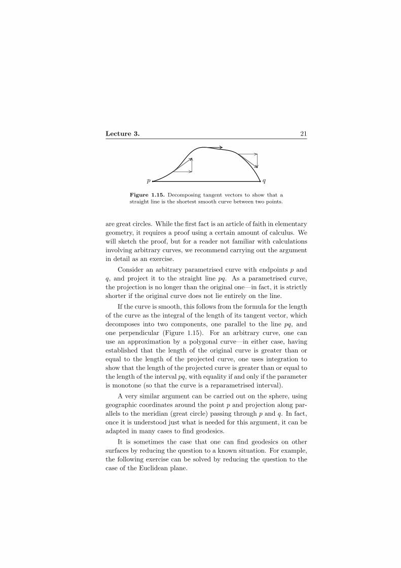
Figure 1.15. Decomposing tangent vectors to show that astraight line is the shortest smooth curve between two points.

are great circles. While the first fact is an article of faith in elementarygeometry, it requires a proof using a certain amount of calculus. Wewill sketch the proof, but for a reader not familiar with calculationsinvolving arbitrary curves, we recommend carrying out the argumentin detail as an exercise.

Consider an arbitrary parametrised curve with endpoints p andq, and project it to the straight line pq. As a parametrised curve,the projection is no longer than the original one—in fact, it is strictlyshorter if the original curve does not lie entirely on the line.

If the curve is smooth, this follows from the formula for the lengthof the curve as the integral of the length of its tangent vector, whichdecomposes into two components, one parallel to the line pq, andone perpendicular (Figure 1.15). For an arbitrary curve, one canuse an approximation by a polygonal curve—in either case, havingestablished that the length of the original curve is greater than orequal to the length of the projected curve, one uses integration toshow that the length of the projected curve is greater than or equal tothe length of the interval pq, with equality if and only if the parameteris monotone (so that the curve is a reparametrised interval).

A very similar argument can be carried out on the sphere, usinggeographic coordinates around the point p and projection along par-allels to the meridian (great circle) passing through p and q. In fact,once it is understood just what is needed for this argument, it can beadapted in many cases to find geodesics.

It is sometimes the case that one can find geodesics on othersurfaces by reducing the question to a known situation. For example,the following exercise can be solved by reducing the question to thecase of the Euclidean plane.


Figure 1.16. Three curves in R3.

Exercise 1.11. Find all geodesics on the round cylinder

{ (x, y, z) $ R3 | x2 + y2 = 1 }

and the upper half of the round cone

{ (x, y, z) $ R3 | x2 + y2 " z2 = 0, z ( 0 }.

c. Parametric representations of curves. We often write a curvein R2 as the solution of a particular equation; the unit circle, for ex-ample, is the set of points satisfying x2 + y2 = 1. This implicitrepresentation becomes more di"cult in higher dimensions; in gen-eral, each equation we require the coordinates to satisfy will removea degree of freedom (assuming independence) and hence a dimension,so to determine a curve in R3 we require not one, but two equations.Geometrically, we are obtaining a curve as the intersection of two sur-faces, each specified by one of the equations. For example, the unitcircle lying in the xy-plane is the solution set of

x2 + y2 = 1

z = 0

which is the intersection of this plane with a cylinder of unit radius.This is a simple example, for which these equations and the visuali-sation of the surfaces pose no real di"culty; there are many exampleswhich are more di"cult to deal with in this manner, but which canbe easily written down using a parametric representation. That is, wedefine the curve in question as the set of all points given by

(x, y, z) = (f1(t), f2(t), f3(t))

Lecture 3. 23

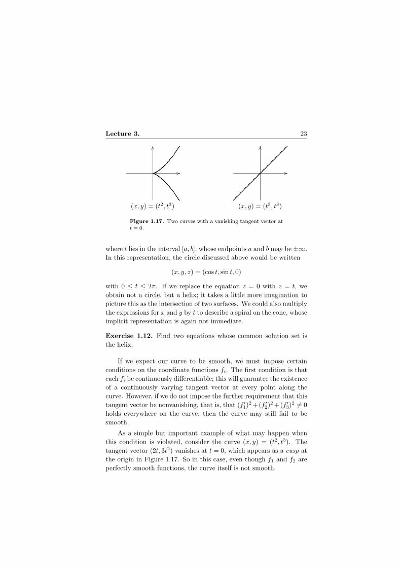
(x, y) = (t2, t3) (x, y) = (t3, t3)

Figure 1.17. Two curves with a vanishing tangent vector att = 0.

where t lies in the interval [a, b], whose endpoints a and b may be ±).In this representation, the circle discussed above would be written

(x, y, z) = (cos t, sin t, 0)

with 0 # t # 2". If we replace the equation z = 0 with z = t, weobtain not a circle, but a helix; it takes a little more imagination topicture this as the intersection of two surfaces. We could also multiplythe expressions for x and y by t to describe a spiral on the cone, whoseimplicit representation is again not immediate.

Exercise 1.12. Find two equations whose common solution set isthe helix.

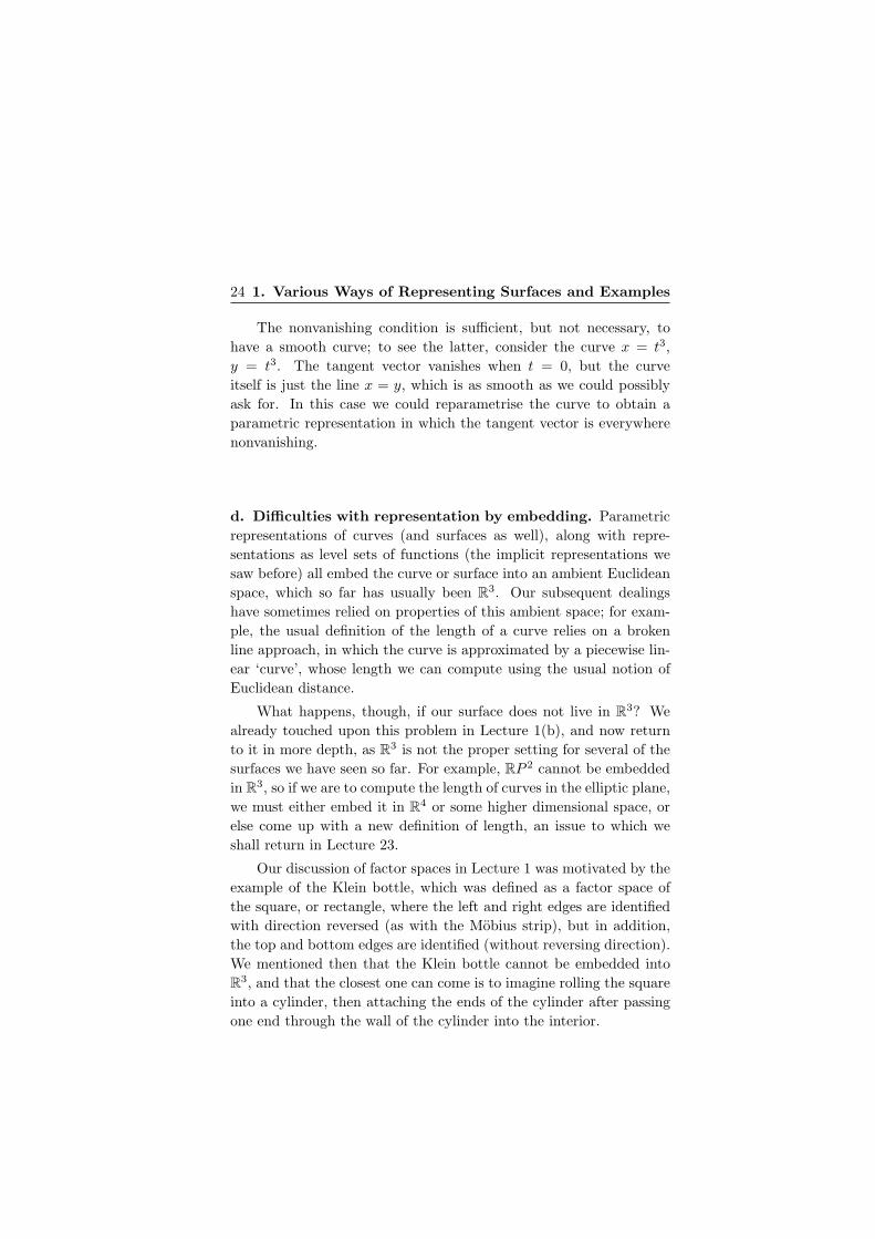
If we expect our curve to be smooth, we must impose certainconditions on the coordinate functions fi. The first condition is thateach fi be continuously di!erentiable; this will guarantee the existenceof a continuously varying tangent vector at every point along thecurve. However, if we do not impose the further requirement that thistangent vector be nonvanishing, that is, that (f !

1)2 +(f !

2)2 +(f !

3)2 != 0

holds everywhere on the curve, then the curve may still fail to besmooth.

As a simple but important example of what may happen whenthis condition is violated, consider the curve (x, y) = (t2, t3). Thetangent vector (2t, 3t2) vanishes at t = 0, which appears as a cusp atthe origin in Figure 1.17. So in this case, even though f1 and f2 areperfectly smooth functions, the curve itself is not smooth.


The nonvanishing condition is su"cient, but not necessary, tohave a smooth curve; to see the latter, consider the curve x = t3,y = t3. The tangent vector vanishes when t = 0, but the curveitself is just the line x = y, which is as smooth as we could possiblyask for. In this case we could reparametrise the curve to obtain aparametric representation in which the tangent vector is everywherenonvanishing.

d. Di!culties with representation by embedding. Parametricrepresentations of curves (and surfaces as well), along with repre-sentations as level sets of functions (the implicit representations wesaw before) all embed the curve or surface into an ambient Euclideanspace, which so far has usually been R3. Our subsequent dealingshave sometimes relied on properties of this ambient space; for exam-ple, the usual definition of the length of a curve relies on a brokenline approach, in which the curve is approximated by a piecewise lin-ear ‘curve’, whose length we can compute using the usual notion ofEuclidean distance.

What happens, though, if our surface does not live in R3? Wealready touched upon this problem in Lecture 1(b), and now returnto it in more depth, as R3 is not the proper setting for several of thesurfaces we have seen so far. For example, RP 2 cannot be embeddedin R3, so if we are to compute the length of curves in the elliptic plane,we must either embed it in R4 or some higher dimensional space, orelse come up with a new definition of length, an issue to which weshall return in Lecture 23.

Our discussion of factor spaces in Lecture 1 was motivated by theexample of the Klein bottle, which was defined as a factor space ofthe square, or rectangle, where the left and right edges are identifiedwith direction reversed (as with the Mobius strip), but in addition,the top and bottom edges are identified (without reversing direction).We mentioned then that the Klein bottle cannot be embedded intoR3, and that the closest one can come is to imagine rolling the squareinto a cylinder, then attaching the ends of the cylinder after passingone end through the wall of the cylinder into the interior.

Lecture 3. 25

Figure 1.18. Life on a dodecahedron.

Of course, this results in the surface intersecting itself in a circle;in order to avoid this self-intersection, we could add a dimension andembed the surface in R4. Given the extra dimension to work with,we could begin with the immersion described above and perform thefour-dimensional analogue of taking a string which is lying in a figureeight on a table, and lifting part of it o! the surface of a table in orderto avoid having it touch itself. No such manoeuvre is possible for theKlein bottle in three dimensions, but the immersion of the Klein bot-tle into R3 is still a popular shape, and some enterprising craftsmanhas been selling both ‘Klein bottles’ and beer mugs in the shape ofKlein bottles at the yearly meetings of the American MathematicalSociety. We had two such glass models of Klein bottles in the class,which were bought there: one is a conventional inverted bottle verysimilar to the image in Figure 1.6; the other is a “Klein beer mug”,very close to a usual one in its outside shape and usable as a drinkingvessel.

Even when an embedding exists, it is possible for the choice ofembedding to obscure certain geometric properties of an object. Con-sider the surface of a dodecahedron (or any solid, for that matter).From the point of view of the embedding in R3, there are three sortsof points on the surface; a given point can lie either at a vertex, alongan edge, or on a face. Being three-dimensional creatures, we see theseas three distinct classes of points.

Now imagine that we are two-dimensional creatures living on thesurface of the dodecahedron. We can tell whether or not we are at


a vertex; at a vertex, the angles add up to less than 2", whereaseverywhere else, they add up to exactly 2". However, we cannottell whether or not we are at an edge; this has to do with the factthat given two points on adjacent faces, the way to find the shortestpath between them is to unfold the two faces and place them flaton the plane (at which stage points on an edge look just like pointson a face), draw a straight line between the two points in question,and then fold the surface back up (Figure 1.18). As far as our two-dimensional selves are concerned, points on an edge and points on aface are indistinguishable, since the unfolding process does not changeany distances along the surface.

It is also possible that a surface which can be embedded in R3 willlose some of its nicer properties in the process. For example, the usualembedding of the torus destroys the symmetry between meridians andparallels; all of the meridians are the same length, but the length ofthe parallels varies. We can retain this symmetry by embedding inR4, the so-called flat torus. Parametrically, this is given by

x = r cos t y = r sin t

z = r cos s w = r sin s

where s, t $ [0, 2"]. As we already mentioned, we can also obtainthe flat torus as a factor space, using the same method as in thedefinition of the projective plane or Klein bottle. Beginning with arectangle, we identify opposite sides (with no reversal of direction);alternately, we can consider the family of isometries of R2 given byTm,n : (x, y) '& (x + m, y + n), where m,n $ Z, and mod out byorbits. This construction of T2 as R2/Z2 is exactly analogous to theconstruction of the circle S1 as R/Z.

We have seen that surfaces can be considered from di!erent view-points: sometimes we treat them as geometric objects, with intrinsi-cally defined distances, angles, and areas, while other times we treatthem as ‘stretchable’ objects which can be bent and deformed, butnot torn or broken. In mathematical language, this corresponds toconsidering di!erent structures on surfaces, and this is the centraltheme of this course, which we will take up in earnest in the nextlecture.

Lecture 3. 27

Before doing so, we would like to fix a linguistic ambiguity; forexample, what should the word ‘sphere’ mean? How will we indicatewhether we are treating a particular surface as a geometric object,or as a topological one (that is, one which may be deformed withoutchanging the nature of the surface)? Our convention will be as follows:an indefinite article in front of the name, as in ‘a sphere’, ‘a torus’ or‘a projective plane’, will mean that we consider the object in the topo-logical sense, up to a homeomorphism. The use of an adjective or thedefinite article will generally signify a smaller class of objects, as in ‘asphere given by an equation’. Then ‘a round sphere’ would mean anysphere which has ‘spherical geometry’, that is, which is isometric tothe actual sphere in Euclidean space. Similarly, ‘a flat torus’ signifiesany torus with locally Euclidean geometry, while ‘the flat torus’ or‘the torus’ will indicate the unit square with opposite sides identified,endowed with the appropriate geometry inherited from R2; sometimeswe will call this object ‘the standard flat torus’. ‘The elliptic plane’indicates the factor space of the unit sphere in which antipodal pointsare identified, with geometry inherited from the sphere, and so on forvarious other examples which will arise.

Exercise 1.13. Write parametric representations for a projectiveplane in each of the following:

(1) R3 (with self-intersections).

(2) R4 (without self-intersections).

e. Regularity conditions for parametrically defined surfaces.A parametrisation of a surface in R3 is given by a region U * R2

with coordinates (t, s) $ U and a set of three maps f1, f2, f3; thesurface is then the image of F = (f1, f2, f3), the set of all points(x, y, z) = (f1(t, s), f2(t, s), f3(t, s)).

As with parametric representations of curves, we need a regular-ity condition to ensure that our surface is in fact smooth, withoutcusps or singularities. We once again require that the functions fi becontinuously di!erentiable, but now it is insu"cient to simply requirethat the matrix of derivatives Df be nonzero. Rather, we require that


it have maximal rank; the matrix is given by

Df =

'

(

#sf1 #tf1

#sf2 #tf2

#sf3 #tf3

)

*

and so our requirement is that the two tangent vectors to the surface,given by the columns of Df , be linearly independent. Under this con-dition, the Implicit Function Theorem guarantees that the parametricrepresentation is locally bijective and that its inverse is di!erentiable.

Parametric representations may of course have singularities. Agood example is the representation of the sphere given by the inversemap to the geographic coordinates, which maps an open disc regularlyonto the sphere with a point removed, and collapses the boundary ofthe disc into this single point.

Lecture 4.

a. Remarks on metric spaces and topology. Geometry in itsmost immediate form deals with measuring distances.8 For this rea-son, metric spaces are fundamental objects in the study of geometry.In the geometric context, the distance function itself is the object ofinterest; this stands in contrast to the situation in analysis, wheremetric spaces are still fundamental (as spaces of functions, for exam-ple), but where the metric is introduced primarily in order to have anotion of convergence, and so the topology induced by the metric isthe primary object of interest, while the metric itself stands somewhatin the background.

A metric space is a set X, together with a metric, or distancefunction, d : X %X & R+

0 , which satisfies the following axioms for allvalues of the arguments:

(1) Positivity: d(x, y) ( 0, with equality i! x = y

(2) Symmetry: d(x, y) = d(y, x)

(3) Triangle inequality: d(x, z) # d(x, y) + d(y, z)

8The reader should be aware, however, that in modern mathematical terminology,the word ‘geometry’ may appear with adjectives like ‘a"ne’ or ‘projective’. Thosebranches of geometry study structures which do not involve distances directly.

Lecture 4. 29

The last of these is generally the most interesting, and is sometimesuseful in the following equivalent form:

d(x, y) ( |d(x, z) " d(y, z)|

Once we have defined a metric on a space X, we immediatelyhave a topology on X induced by that metric. The ball in X withcentre x and radius r is given by

B(x, r) = { y $ X | d(x, y) < r }

Then a set A * X is said to be open if for every x $ A, there existsr > 0 such that B(x, r) * A, and A is closed if its complement X \Ais open. We now have two equivalent notions of convergence: in themetric sense, xn & x if d(xn, x) & 0, while the topological definitionrequires that for every open set U containing x, there exist some Nsuch that for every n > N , we have xn $ U . It is not hard to see thatthese are equivalent.

Similarly for the definition of continuity; we say that a functionf : X & Y is continuous if xn & x implies f(xn) & f(x). Theequivalent definition in more topological language is that continuityrequires f"1(U) * X to be open whenever U * Y is open. We saythat f is a homeomorphism if it is a bijection and if both f and f"1

are continuous.

Exercise 1.14. Show that the two sets of definitions (metric andtopological) in the previous two paragraphs are equivalent.

Within mathematics, there are two broad categories of conceptsand definitions with which we are concerned. In the first instance, weseek to fully describe and understand a particular sort of structure.We make a particular definition or construction, and then seek toeither show that there is only one object (up to some appropriatenotion of isomorphism) which fits our definition, or to give some sortof classification which exhausts all the possibilities. Examples of thisapproach include Euclidean space, which is unique once we specifydimension, or Jordan normal form, which is unique for a given matrixup to a permutation of the basis vectors, as well as finite simplegroups, or semi-simple Lie algebras, for which we can (eventually)obtain a complete classification.


No such uniqueness or classification result is possible with metricspaces and topological spaces in general; these definitions are exam-ples of the second sort of mathematical object, and are generalitiesrather than specifics. In and of themselves, they are far too generalto allow any sort of complete classification or universal understand-ing, but they have enough properties to allow us to eliminate muchof the tedious case by case analysis which would otherwise be nec-essary when proving facts about the objects in which we are reallyinterested. The general notion of a group, or of a Banach space, alsofalls into this category of generalities.

Before moving on, there are three definitions of which we oughtto remind ourselves. First, recall that a metric space is complete ifevery Cauchy sequence converges. This is not a purely topologicalproperty, since we need a metric in order to define Cauchy sequences;to illustrate this fact, notice that the open interval (0, 1) and the realline R are homeomorphic, but that the former is not complete, whilethe latter is.

Secondly, we say that a metric space (or subset thereof) is com-pact if every sequence has a convergent subsequence. In the context ofgeneral topological spaces, this property is known as sequential com-pactness, and the definition of compactness is given as the require-ment that every open cover have a finite subcover; for our purposes,since we will be dealing with metric spaces, the two definitions areequivalent. There is also a notion of precompactness, which requiresevery sequence to have a Cauchy subsequence.

The knowledge that X is compact allows us to draw a numberof conclusions; the most commonly used one is that every continuousfunction f : X & R is bounded, and in fact achieves its maximumand minimum. In particular, the product space X % X is compact,and so the distance function is bounded.

Finally, we say that X is connected if it cannot be written asthe union of non-empty disjoint open sets; that is, X = A + B, Aand B open, A , B = - implies either A = X or B = X. There isalso a notion of path connectedness, which requires for any two pointsx, y $ X the existence of a continuous function f : [0, 1] & X suchthat f(0) = x and f(1) = y. As is the case with the two forms of

Lecture 4. 31

compactness above, these are not equivalent for arbitrary topologicalspaces (or even for arbitrary metric spaces—the usual counterexampleis the union of the graph of sin(1/x) with the vertical axis), but willbe equivalent on the class of spaces with which we are concerned.

b. Homeomorphisms and isometries. In the topological context,the natural notion of equivalence between two spaces is that of home-omorphism, which we defined above as a continuous bijection withcontinuous inverse. Two topological spaces are homeomorphic if thereexists a homeomorphism between them. Any property common to allhomeomorphic spaces is called a topological invariant ; this naturallyincludes any property defined in purely topological terms, such asconnectedness, path-connectedness, and compactness.

Some invariants require a little more work; for example, we wouldlike to believe that dimension is a topological invariant, and this isin fact true,9 but proving that Rm and Rn are not homeomorphic form != n requires non-trivial tools.

A considerable part of this course deals with topological invari-ants of compact surfaces, and in particular, the task of classifyingsuch surfaces up to a homeomorphism. We will almost succeed insolving this problem completely; the only assumption we will haveto make is that the surfaces in question admit one of several naturaladditional structures. In fact this assumption turns out to be true forany surface, but we do not prove this in this course.

The natural equivalence relation in the geometric setting is isom-etry; a map f : X & Y between metric spaces is isometric if

dY (f(x1), f(x2)) = dX(x1, x2)

for every x1, x2 $ X. If in addition f is a bijection, we say f is anisometry. We are particularly interested in the set of isometries fromX to itself,

Isom(X, d) = { f : X & X | f is an isometry }

which we can think of as the symmetries of X. In general, the moresymmetric X is, the larger this set.

9At least for the usual definition of dimension; we mention an alternate definitionin the next section.


Figure 1.19. A planar model on a hexagon.

In fact, Isom(X, d) is not just a set; it has a natural binary op-eration given by composition, under which is becomes a group. Thisis an example of a very natural and general sort of group which isoften of interest; all the bijections from some fixed set to itself, withcomposition as the group operation. On a finite set, this gives thesymmetric group Sn, the group of permutations. On an infinite set,the group of all bijections becomes somewhat unwieldy, and it is morenatural to consider the subgroup of bijections which preserve a partic-ular structure, in this case the metric structure of the space. Anothercommon example of this is the general linear group GL(n, R), whichis the group of all bijections from Rn to itself preserving the linearstructure of the space.

In the next lecture, we will discuss the isometry groups of Eu-clidean space and of the sphere.

Exercise 1.15. Consider a regular hexagon with pairs of oppositesides identified by the corresponding translations, as in Figure 1.19.

(1) Prove that it is a torus.

(2) Prove that locally, it is isometric to Euclidean plane.

(3) Prove that it is not isometric to the standard flat torus.

c. Other notions of dimension. As mentioned above, we usuallythink of dimension as a topological invariant. However, for generalcompact metric spaces there is another notion of dimension which isa metric invariant, rather than a topological one. The main idea isto capture the rate at which volume (or some other sort of measure)scales with the metric; for example, a cube in Rn with side length rhas volume rn, and the exponent n is the dimension of the space.

Lecture 4. 33

In general, given a compact metric space X, for any $ > 0, letN($) be the minimum number of $-balls required to cover X; thatis, the minimum number of points x1, . . . , xN(!) in X such that everypoint in X lies within $ of some xi. This may be thought of asmeasuring the average ‘volume’ of an $-ball, in some sense; the upperbox dimension of X is defined to be

dbox(X) = lim sup!#0

log N($)

log 1/$.

We take the upper limit because the limit itself may not exist. Thelower box dimension is defined similarly, taking the lower limit in-stead. These notions of dimension do not behave quite as nicely aswe would like in all situations; for example, the set of rational num-bers, which is countable, has upper and lower box dimension equal toone.

There is a more e!ective notion of Hausdor! dimension, whicheliminates the need to distinguish between upper and lower limits,and which is equal to zero for any countable set; because its definitionrequires an understanding of measure theory, we will not discuss ithere. For ‘good’ sets all three definitions coincide, and are centralto the study of fractal geometry; however, they are not topologicalinvariants, so our claim in the last section must be understood toapply only to a strictly topological notion of dimension.

d. Geodesics. When we are interested in a metric space as a geo-metric object, rather than as something in analysis or topology, it isof particular interest to examine those triples (x, y, z) for which thetriangle inequality becomes degenerate, that is, for which d(x, z) =d(x, y) + d(y, z).

For example, if our space X is just the Euclidean plane R2 withdistance function given by Pythagoras’ formula,

d((x1, x2), (y1, y2)) =$

(y1 " x1)2 + (y2 " x2)2

then the triangle inequality is a consequence of the Cauchy-Schwarzinequality, and we have equality in the one i! we have equality in theother; this occurs i! y lies in the line segment [x, z], so that the threepoints x, y, z are in fact collinear.


x

yz

dxy

dyz

dxzIx

Iy

z1

z2dxz

dyz

Figure 1.20. Images of three points determine an isometry.

A similar observation holds on the sphere, where the triangleinequality becomes degenerate for the triple (x, y, z) i! y lies alongthe shorter arc of the great circle connecting x and z. So in boththese cases, degeneracy occurs when the points lie along a geodesic;this suggests that in general, a characteristic property of a geodesicis the relation d(x, z) = d(x, y) + d(y, z) whenever y lies between twopoints x and z which are su"ciently close along the curve.

Lecture 5.

a. Isometries of the Euclidean plane. There are three ways todescribe and study isometries of the Euclidean plane: synthetic; asa"ne maps in two real dimensions; and as a"ne maps in one complexdimension. The last two methods are closely related. We begin withobservations using the traditional synthetic approach.

If we fix three noncollinear points in R2 and want to describe thelocation of a fourth, it is enough to know its distance from each of thefirst three. This may readily be seen from the fact that three circleswhose centres are not collinear intersect in at most one point.

As a consequence of this, an isometry of R2 is completely de-termined by its action on three noncollinear points. In fact, if wehave an isometry I : R2 & R2, and three such points x, y, z, as inFigure 1.20, the choice of Ix constrains Iy to lie on the circle withcentre Ix and radius d(x, y), and once we have chosen Iy, there areonly two possibilities for Iz; one (z1) corresponds to the case where Ipreserves orientation, the other (z2) to the case where orientation is

Lecture 5. 35

x = Ix

y

z

Iy

Iz

Rotation—one fixed point

x

y

z

Ix

Iy

Iz

Translation—no fixed points

Figure 1.21. Orientation preserving isometries.

reversed. So for two pairs of distinct points a, b and a!, b! such thatthe distances between a and b and between a! and b! coincide, thereare exactly two isometries which map a to a! and b to b!; one of thesewill be orientation preserving, the other orientation reversing.

Passing to algebraic descriptions, notice that any isometry I mustcarry lines to lines, since as we saw last time, three points in the planeare collinear i! the triangle inequality becomes degenerate. Thusit is an a"ne map—that is, a composition of a linear map and atranslation—so it may be written as I : x '& Ax + b, where b $ R2

and A is a 2% 2 matrix. In fact, A must be orthogonal, which meansthat we can write things in terms of the complex plane C and get (inthe orientation preserving case) I : z '& az + b, where a, b $ C and|a| = 1. In the orientation reversing case, we have I : z '& az + b.

Using the preceding discussion, we can now classify any isometryof the Euclidean plane as belonging to one of four types, dependingon whether it preserves or reverses orientation, and whether or not ithas a fixed point.

Case 1 : An orientation preserving isometry which possesses afixed point is a rotation. Let x be the fixed point, Ix = x. Fixanother point y; both y and Iy lie on a circle of radius d(x, y) aroundx. The rotation about x which takes y to Iy satisfies these criteria,which are enough to uniquely determine I given that it preservesorientation, hence I is exactly this rotation.


a

Iab

Ibc = Ic

a

Ia b

Ib

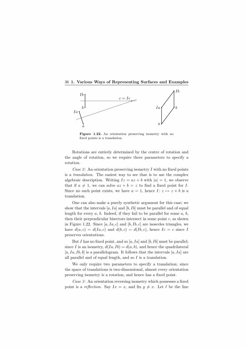
Figure 1.22. An orientation preserving isometry with nofixed points is a translation.

Rotations are entirely determined by the centre of rotation andthe angle of rotation, so we require three parameters to specify arotation.

Case 2 : An orientation preserving isometry I with no fixed pointsis a translation. The easiest way to see that is to use the complexalgebraic description. Writing Iz = az + b with |a| = 1, we observethat if a != 1, we can solve az + b = z to find a fixed point for I.Since no such point exists, we have a = 1, hence I : z '& z + b is atranslation.

One can also make a purely synthetic argument for this case; weshow that the intervals [a, Ia] and [b, Ib] must be parallel and of equallength for every a, b. Indeed, if they fail to be parallel for some a, b,then their perpendicular bisectors intersect in some point c, as shownin Figure 1.22. Since [a, Ia, c] and [b, Ib, c] are isosceles triangles, wehave d(a, c) = d(Ia, c) and d(b, c) = d(Ib, c), hence Ic = c since Ipreserves orientations.

But I has no fixed point, and so [a, Ia] and [b, Ib] must be parallel;since I is an isometry, d(Ia, Ib) = d(a, b), and hence the quadrilateral[a, Ia, Ib, b] is a parallelogram. It follows that the intervals [a, Ia] areall parallel and of equal length, and so I is a translation.

We only require two parameters to specify a translation; sincethe space of translations is two-dimensional, almost every orientationpreserving isometry is a rotation, and hence has a fixed point.

Case 3 : An orientation reversing isometry which possesses a fixedpoint is a reflection. Say Ix = x, and fix y != x. Let % be the line

Lecture 5. 37

x = Ix

y

z

Iy

Iz

x

y

z Ix

Iy

Iz

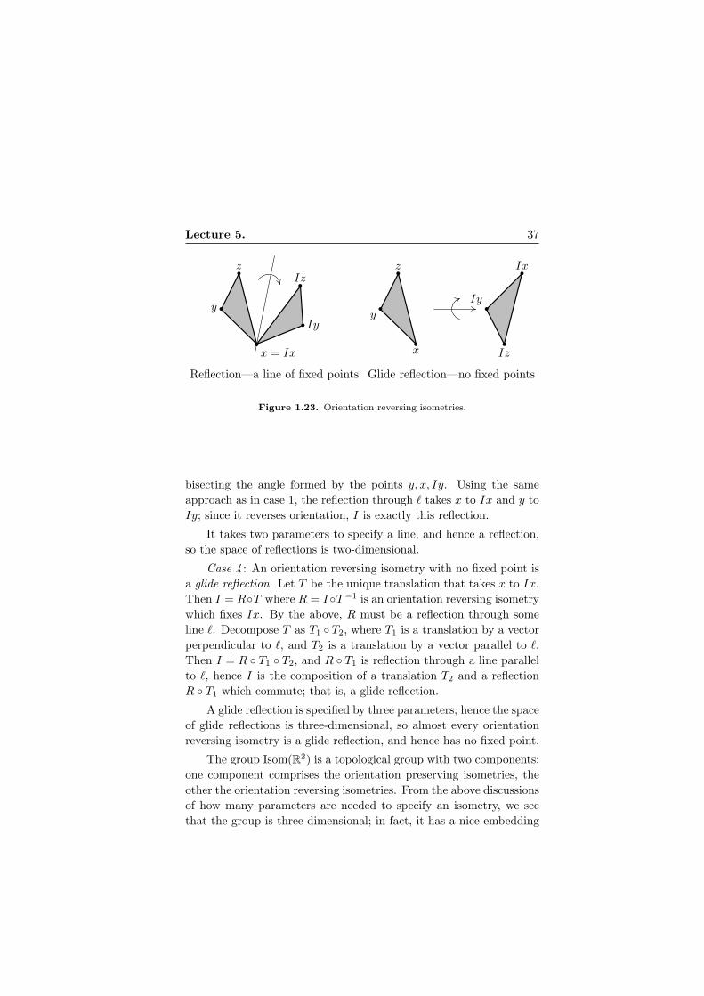
Reflection—a line of fixed points Glide reflection—no fixed points

Figure 1.23. Orientation reversing isometries.

bisecting the angle formed by the points y, x, Iy. Using the sameapproach as in case 1, the reflection through % takes x to Ix and y toIy; since it reverses orientation, I is exactly this reflection.

It takes two parameters to specify a line, and hence a reflection,so the space of reflections is two-dimensional.

Case 4 : An orientation reversing isometry with no fixed point isa glide reflection. Let T be the unique translation that takes x to Ix.Then I = R.T where R = I.T"1 is an orientation reversing isometrywhich fixes Ix. By the above, R must be a reflection through someline %. Decompose T as T1 . T2, where T1 is a translation by a vectorperpendicular to %, and T2 is a translation by a vector parallel to %.Then I = R . T1 . T2, and R . T1 is reflection through a line parallelto %, hence I is the composition of a translation T2 and a reflectionR . T1 which commute; that is, a glide reflection.

A glide reflection is specified by three parameters; hence the spaceof glide reflections is three-dimensional, so almost every orientationreversing isometry is a glide reflection, and hence has no fixed point.

The group Isom(R2) is a topological group with two components;one component comprises the orientation preserving isometries, theother the orientation reversing isometries. From the above discussionsof how many parameters are needed to specify an isometry, we seethat the group is three-dimensional; in fact, it has a nice embedding


into the group GL(3, R) of invertible 3 % 3 matrices:

Isom(R2) =

+,

O(2) R2

0 1

-

:

,

R2

1

-

&,

R2

1

-.

.

Here O(2) is the group of real valued orthogonal 2 % 2 matrices, andthe plane upon which Isom(R2) acts is the horizontal plane z = 1 inR3.

Exercise 1.16. Prove that every isometry of the Euclidean plane canbe represented as a product of at most three reflections.

Exercise 1.17. Consider all possible configurations of two and threelines in the plane: two lines may be either parallel or intersecting;for three lines there are a few more options. Identify the product ofreflections in those lines for each case as one of four types of isometries.

Exercise 1.18. Consider an orientation reversing isometry in thecomplex form z '& az + b. Find a condition on a, b $ C which willdetermine if it is a reflection or a glide reflection, and identify the axisin both cases.

b. Isometries of the sphere and the elliptic plane. By countingdimensions in the isometry group of the Euclidean plane, we arguedthat almost every orientation preserving isometry has a fixed point,while almost every orientation reversing isometry has no fixed point.In the next lecture, we will see that the picture for the sphere issomewhat similar—now any orientation preserving isometry has afixed point, and most orientation reversing ones have none. For theelliptic plane, however, it will turn out to be dramatically di!erent:any isometry has a fixed point, and can in fact be interpreted as arotation!

Many of the arguments in the previous section carry over to thesphere; the same techniques of taking intersections of circles, etc.still apply. The classification of isometries on the sphere is somewhatsimpler, since every orientation preserving isometry has a fixed point,while every orientation reversing isometry (other than reflection in agreat circle) has a point of period two, which becomes a fixed pointwhen we pass to the elliptic plane.

Lecture 6. 39

We will be able to show that every orientation preserving isometryof the sphere comes from a rotation of R3, and that the product oftwo rotations is itself a rotation. This is slightly di!erent from thecase with Isom(R2), where the product could either be a rotation, orif the two angles of rotation summed to zero (or a multiple of 2"), atranslation. We will, in fact, be able to obtain Isom(S2) as a group of3% 3 matrices in a much more natural way than we did for Isom(R2)above, since any isometry of S2 extends to a linear orthogonal mapof R3, and so we will be able to use linear algebra directly.

Lecture 6.

a. Classification of isometries of the sphere and the ellipticplane. There are two approaches we can take to investigating isome-tries of the sphere S2; we saw this dichotomy begin to appear whenwe examined Isom(R2). The first is the synthetic approach, whichtreats the problem using the tools of solid geometry; this is the ap-proach used by the Greek geometers of late antiquity in developingspherical geometry for use in astronomy.

The second approach, which we will follow below, uses methods oflinear algebra; translating the question about geometry to a questionabout matrices puts a wide range of techniques at our disposal, whichwill prove enlightening, and rather more useful now than it was in thecase of the plane, when the relevant matrices were only 2 % 2.

The first important result is that there is a natural bijection(which is in fact a group isomorphism) between Isom(S2) and O(3),the group of real orthogonal 3 % 3 matrices. The latter is defined by

O(3) = {A $ M3(R) | AT A = I }

That is, O(3) comprises those matrices for which the transpose andthe inverse coincide. This has a nice geometric interpretation; wecan think of the columns of a 3 % 3 matrix as vectors in R3, so thatA = (a1|a2|a3), where ai $ R3. (In fact, ai is the image of the ith basisvector ei under the action of A). Then A lies in O(3) i! {a1, a2, a3}forms an orthonormal basis for R3, that is, if /ai, aj0 = &ij , where /·, ·0denotes inner product, and &ij is the Kronecker delta, which takes the


value 1 if i = j, and 0 otherwise. The same criterion applies if weconsider the rows of A, rather than the columns.

Since det(AT ) = det(A), any matrix A $ O(3) has determi-nant ±1; the sign of the determinant indicates whether the map pre-serves or reverses orientation. The group of real orthogonal matriceswith determinant equal to positive one is the special orthogonal groupSO(3).

In order to see that the members of O(3) are in fact the isometriesof S2, we could take the synthetic approach and look at the imagesof three points not all lying on the same geodesic, as we did withIsom(R2); in particular, the standard basis vectors e1, e2, e3.

An alternate approach is to extend the isometry to R3 by ho-mogeneity. That is, given an isometry I : S2 & S2, we can define alinear map A : R3 & R3 by

Ax = 1x1 · I,

x

1x1

-

It follows that A preserves lengths in R3, and in fact, this is su"cientto show that it preserves angles as well. This can be seen using atechnique called polarisation, which allows us to express the innerproduct in terms of the norm, and hence show the general result thatpreservation of norm implies preservation of inner product:

1x + y12 = /x + y, x + y0= /x, x0 + 2/x, y0 + /y, y0

= 1x12 + 1y12 + 2/x, y0

/x, y0 =1

2(1x + y12 " 1x12 " 1y12)

This is a useful trick to remember, and allows us to show that asymmetric bilinear form is determined by its diagonal part. In ourparticular case, it shows that the matrix A we obtained is in fact inO(3), since it preserves both lengths and angles.

The matrix A $ O(3) has three eigenvalues, some of which may becomplex. Because A is orthogonal, we have |'| = 1 for each eigenvalue'; further, because the determinant is the product of the eigenvalues,we have '1'2'3 = ±1. The entries of the matrix A are real, hence the

Lecture 6. 41

coe"cients of the characteristic polynomial are as well; this impliesthat if ' is an eigenvalue, so is its complex conjugate '.

There are two cases to consider. Suppose det(A) = 1. Then theeigenvalues are ', ', and 1, where ' = ei" lies on the unit circle inthe complex plane. Let x be the eigenvector corresponding to theeigenvalue 1, and note that A acts on the plane orthogonal to x byrotation by (; hence A is a rotation by ( around the axis through x.

The second case, det(A) = "1, can be dealt with by noting that Acan be written as a composition of "I (reflection through the origin)with a matrix with positive determinant, which must be a rotation,by the above discussion. Upon passing to the elliptic plane RP 2, thereflection "I becomes the identity, so that every isometry of RP 2 isa rotation.

This result, that every isometry of the sphere is either a rotationor the composition of a rotation and a reflection through the origin,shows that every isometry has either a fixed point or a point of periodtwo, which becomes a fixed point upon passing to the quotient spaceRP 2.

As an concrete example of how all isometries become rotations inRP 2, consider the map A given by reflection through the xy-plane,A(x, y, z) = (x, y,"z). Let R be rotation by " about the z-axis, givenby R(x, y, z) = ("x,"y, z). Then A = R . ("I), so that as maps onRP 2, A and R coincide. Further, any point (x, y, 0) on the equatorof the sphere is fixed by this map, so that R fixes not only one pointin RP 2, but many.

Exercise 1.19. Let x and y be two points in the elliptic plane.

(1) Prove that there are at most two shortest curves connectingx and y.

(2) Find a necessary and su"cient condition for uniqueness ofthe shortest curve connecting x and y.

b. Area of a spherical triangle. In the Euclidean plane, the mostsymmetric formula for determining the area of a triangle is Heron’sformula

A =$

s(s " a)(s " b)(s " c)


Figure 1.24. Determining the area of a spherical triangle.

where a, b, c are the lengths of the sides, and s = 12 (a + b + c) is

the semiperimeter of the triangle. There are other, less symmetric,formulas available to us if we know the lengths of two sides and themeasure of the angle between them, or two angles and a side; if allwe have are the angles, however, we cannot determine the area, sincethe triangle could be scaled up or down, preserving the angles whilechanging the area.

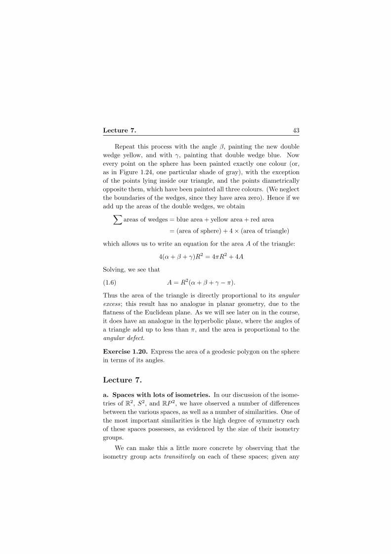
This is not the case on the surface of the sphere; given a sphericaltriangle, that is, the area on the sphere enclosed by three geodesics(great circles), we can find the area of the triangle via a wonderfullyelegant formula in terms of the angles, as follows.

Consider the ‘wedge’ lying between two lines of longitude on thesurface of a sphere, with an angle ( between them. The area ofthis wedge is proportional to (, and since the surface area of thesphere with radius R is 4"R2, it follows that the area of the wedgeis "

2# 4"R2 = 2(R2. If we take this together with its mirror image(upon reflection through the origin), which lies on the other side ofthe sphere, runs between the same poles, and has the same area, thenthe area of the ‘double wedge’ shown in Figure 1.24 is 4(R2.

Now consider a spherical triangle with angles (, ), and !. Putthe vertex with angle ( at the north pole, and consider the doublewedge lying between the two great circles which form the angle (.Paint this double wedge red; as we saw above, it has area 4(R2.

Lecture 7. 43

Repeat this process with the angle ), painting the new doublewedge yellow, and with !, painting that double wedge blue. Nowevery point on the sphere has been painted exactly one colour (or,as in Figure 1.24, one particular shade of gray), with the exceptionof the points lying inside our triangle, and the points diametricallyopposite them, which have been painted all three colours. (We neglectthe boundaries of the wedges, since they have area zero). Hence if weadd up the areas of the double wedges, we obtain

/

areas of wedges = blue area + yellow area + red area

= (area of sphere) + 4 % (area of triangle)

which allows us to write an equation for the area A of the triangle:

4(( + ) + !)R2 = 4"R2 + 4A

Solving, we see that

(1.6) A = R2(( + ) + ! " ").

Thus the area of the triangle is directly proportional to its angularexcess; this result has no analogue in planar geometry, due to theflatness of the Euclidean plane. As we will see later on in the course,it does have an analogue in the hyperbolic plane, where the angles ofa triangle add up to less than ", and the area is proportional to theangular defect.

Exercise 1.20. Express the area of a geodesic polygon on the spherein terms of its angles.

Lecture 7.

a. Spaces with lots of isometries. In our discussion of the isome-tries of R2, S2, and RP 2, we have observed a number of di!erencesbetween the various spaces, as well as a number of similarities. One ofthe most important similarities is the high degree of symmetry eachof these spaces possesses, as evidenced by the size of their isometrygroups.

We can make this a little more concrete by observing that theisometry group acts transitively on each of these spaces; given any


two points a and b in the plane, on the sphere, or in the projectiveplane, there is an isometry I of the space such that Ia = b.

In fact, we can make the stronger observation that the group actstransitively on the set of unit tangent vectors. That is to say, if v isa unit tangent vector at a, which can be thought of as indicating aparticular direction along the surface from the point a, and w is aunit tangent vector at b, then not only can we find an isometry thatcarries a to b, but we can find one that carries v to w.

Another example of a surface with this property is the hyper-bolic plane, which will appear in Chapter 4, and has the remarkableproperty that its isometry group allows not one but three naturalrepresentations as a matrix group (or a factor of such a group by itstwo-element centre).

In fact, these four examples are the only surfaces for which isome-tries act transitively on unit tangent vectors. There are of course anumber of higher-dimensional spaces with this property: Euclideanspaces, spheres, and projective spaces, which are all analogues of theirtwo-dimensional counterparts, immediately come to mind, and thereare many more besides.

As an example of a space for which this property fails, considerthe flat torus T2 = R2/Z2. The property holds locally, in the neigh-bourhood of a point, but does not hold on the entire space. WhileIsom(T2) acts transitively on points, it does not act transitively ontangent vectors; some directions lie along geodesics which are closedcurves, while other directions do not. Another example is given bythe cylinder, and examples of a di!erent nature will appear later whenwe consider the hyperbolic plane and its factors.

What sorts of isometries does T2 have? We may consider trans-lations z '& z + z0; rotations of R2, however, will not generally leadto isometries of T2, since they will usually fail to preserve the latticeZ2. The rotation by "/2 about the origin is permissible, as are theflips around the x- and y-axes, and around the line x = y.

In general, Z2 must be mapped to itself or a translation of itself,and so the isometry group is generated by the group of translations,along with the symmetry group of the lattice. The latter group is

Lecture 7. 45

simply D4, the dihedral group on four letters, which arises as thesymmetry group of the square.

Exercise 1.21. Describe all the isometries of

(1) the ‘hexagonal’ torus of Exercise 1.15;

(2) the flat Mobius strip;

(3) the flat Klein bottle, i.e. the square with appropriately iden-tified pairs of opposite sides.

Consider a more general class of examples, which generalise theconstruction of the flat torus as R2/Z2. Let L be a lattice in R2—thatis, a set of vectors of the form {mu + nv | m,n $ Z }, where u and vare two fixed linearly independent vectors. We can identify the factorspace R2/L with the parallelogram

{ su + tv | 0 # s, t # 1 }

with pairs of opposite sides identified by translations.

Exercise 1.22. Show that the following statements hold.

(1) The factor space R2/L is homeomorphic to a torus;

(2) R2/L has a natural metric which is locally isometric to R2;

(3) The isometry group acts transitively on R2/L.

The ‘crystallographic restriction’ property established in the fol-lowing exercise aids in the classification of isometries of these tori.

Exercise 1.23. Show that any nontrivial isometry of R2/L with afixed point has period 2, 3, 4, or 6.

b. Symmetric spaces. The discussion of spaces with lots of isome-tries is related to the notion of a symmetric space, which we will nowexamine more closely. In what follows, we assume certain propertiesof geodesics which will be formally described (but not proved) later inthis course. In particular, we assume that there is a unique geodesicpassing through a given point in a given direction, and that there is aunique shortest geodesic connecting any two su"ciently close points.


Of course, all of this assumes the metric on our surface is given in anice way, as has been the case with all examples considered so far.10

Given a point x on a surface X, we define the geodesic flip throughx, denoted by Ix, as follows. For each geodesic ! passing through x,each point y lying on ! is sent to the point on ! which is the samedistance along the geodesic from x as y is, but in the other direc-tion. It is immediate that this map preserves lengths along geodesicsthrough x; it may happen, however, that the distances between thesegeodesics vary, in which case the map would not be isometric.

If the map is indeed isometric on some neighbourhood of x, and ifthis property holds for the geodesic flip Ix through any point x $ X,then we say that X is locally symmetric. The classification of suchspaces (in any dimension) is one of the triumphs of Lie theory. No-tice that the geodesic flip may not be extendable to a globally definedisometry, so the isometry group of a locally symmetric space may be(and sometimes is) quite small. Although we have not yet encoun-tered any such examples, later on (Lecture 31) we will construct thehyperbolic octagon, whose isometry group can be shown to be finite,even though the space is locally symmetric.

Given two nearby points x, y, we can take the point z lying at themidpoint of the geodesic segment connecting them. Then Izx = y.If X is connected (and hence path connected) then any two pointscan be connected by a finite chain of neighbourhoods where theselocal isometries are defined. This implies that for any two points ina locally symmetric space, there exists an isometry between smallenough neighbourhoods of those points. In other words, locally sucha space looks the same near every point.

If for any point x $ X the geodesic flip Ix can be defined not justlocally, but globally (that is, extended to the entire surface X), andif it is in fact an isometry of X, then we say X is globally symmetric.In this case, the group of isometries Isom(X) acts transitively on allof X.

10These notions of direction and ‘nice’ metrics, which are rather vague at themoment, will be made more precise when we discuss smooth manifolds and Riemannianmetrics in Chapters 3 and 4.

Lecture 7. 47

In the previous lecture we discussed a related, but stronger, no-tion, in which we require Isom(X) to act transitively not only onpoints in X, but also on unit tangent vectors. If this holds, then inparticular, given any x $ X, there is an isometry of X taking sometangent vector at x to its opposite; this isometry must then be thegeodesic flip, and so X is globally symmetric. It is not the case,however, that every globally symmetric space has this property oftransitive action on tangent vectors; the flat torus is one example.

Examples of symmetric spaces are given by Rn, Sn, and RPn,as well as by their direct products, about which we will say moremomentarily. First, notice that the flat torus is symmetric, being thedirect product of two symmetric spaces S1. However, the embeddingof the torus into R3 produces a space which is not symmetric, sincethe isometry group does not act transitively on the points of the sur-face. In fact, the isometry group of the embedded torus of revolution(the bagel) in R3 is a finite extension of a one-dimensional group ofrotations, while the isometry group of the flat torus is, as we saw lasttime, a finite extension of a two-dimensional group of translations.Hence the two surfaces are homeomorphic but not isometric.

The flat torus R2/Z2 has no isometric embedding into R3, but itis isometric to the embedded torus in R4 given as the zero set of thetwo equations

x21 + x2

2 = 1

x23 + x2

4 = 1.

c. Remarks concerning direct products. Given any two sets Xand Y , we can define their direct product, sometimes called the Carte-sian product, as the set of all ordered pairs (x, y):

X % Y = { (x, y) | x $ X, y $ Y }

It is very often the case that if X and Y carry an extra structure,such as that of a group, a topological space, or a metric space, thenthis structure can be carried over to the direct product in a naturalway. For example, the direct product of two groups is a group underpointwise multiplication, and the direct product of two topologicalspaces is a topological space in the product topology.


If X and Y carry metrics dX and dY , then we can put a metricon X % Y in the same manner as we put a metric on R2, by defining

d((x, y), (x!, y!)) =$

dX(x, x!)2 + dY (y, y!)2

If there are geodesics on X and Y , we can define geodesics on X %Y ,and hence can define the geodesic flip, which can be shown to satisfythe formula

I(x,y)(x!, y!) = (Ix(x!), Iy(y!))

In the case R % R = R2, this corresponds to the fact that the com-position of a flip about a vertical line with a flip about a horizontalline is equivalent to rotation by " around the intersection of the twolines.

With the geodesic flip defined, we can then ask whether the prod-uct space X % Y is symmetric, and it turns out that if X and Y areboth symmetric spaces, so is their direct product X % Y . In thismanner we can obtain many higher-dimensional examples, and so ifwe were to attempt to classify such spaces, we would want to focuson those which are irreducible in that they cannot be decomposed asthe direct product of two lower-dimensional spaces, since the otherexamples will be built from these.

The direct product provides a common means by which we de-compose objects of interest into simpler examples in order to gaina complete understanding. We find many examples of this in linearalgebra, in which context the phrase direct sum is also sometimesused. Any finite-dimensional vector space can be written as the di-rect product of n copies of R; this is just the statement that anyfinite-dimensional vector space has a basis. A more sophisticated ap-plication of this process is the decomposition of a linear transforma-tion in terms of its action upon its eigenspaces, so that a symmetricmatrix can be written as the direct product of one-dimensional trans-formations, while for a general matrix, we have the Jordan normalform.

This process is also used in the classification of finitely generatedabelian groups, where we decompose the group of interest into a directsum of copies of Z and cyclic groups whose order is a power of aprime, so that no further decomposition is possible. Thus the natural

Lecture 7. 49

counterpart to the study of how a particular sort of mathematicalstructure can be decomposed is the study of what instances of thatstructure are, in some appropriate sense, irreducible.

various ways of representing surfaces and basic examples

Documents