vector calculus 2016-17 notes - university of readingst904897/vc2016/vectorcalculus_lectu… · a....
TRANSCRIPT

Vector Calculus
Andrea Moiola
University of Reading, 19th September 2016
These notes are meant to be a support for the vector calculus module (MA2VC/MA3VC) taking placeat the University of Reading in the Autumn term 2016.
The present document does not substitute the notes taken in class, where more examples andproofs are provided and where the content is discussed in greater detail.
These notes are self-contained and cover the material needed for the exam. The suggested textbookis [1] by R.A. Adams and C. Essex, which you may already have from the first year; several copies areavailable in the University library. We will cover only a part of the content of Chapters 10–16, moreprecise references to single sections will be given in the text and in the table in Appendix G. This bookalso contains numerous exercises (useful to prepare the exam) and applications of the theory to physicaland engineering problems. Note that there exists another book by the same authors containing the workedsolutions of the exercises in the textbook (however, you should better try hard to solve the exercises and, ifunsuccessful, discuss them with your classmates). Several other good books on vector calculus and vectoranalysis are available and you are encouraged to find the book that suits you best. In particular, SergeLang’s book [5] is extremely clear. [7] is a collection of exercises, many of which with a worked solution(and it costs less than 10£). You can find other useful books on shelf 515.63 (and those nearby) in theUniversity library. The lecture notes [2], the book [3] and the “Vector Calculus Primer” [6] are availableonline; on the web page [4] of O. Knill you can find plenty of exercises, lecture notes and graphs. Note thatdifferent books inevitably use different notation and conventions. In this notes we will take for grantedwhat you learned in the previous classes, so the first year notes might be useful from time to time (inparticular those for calculus, linear algebra and analysis).
Some of the figures in the text have been made with Matlab. The scripts used for generating theseplots are available on Blackboard and on the web page1 of the course; most of them can be run in Octaveas well. You can use and modify them: playing with the different graphical representations of scalar andvector fields is a great way to familiarise with these concepts. On the same page you can find the fileVCplotter.m, which you can use to visualise fields, curves and changes of variables in Matlab or Octave.
Warning 1: The paragraphs and the proofs marked with a star “⋆” are addressed to students willingto deepen the subject and learn about some closely related topics. Some of these remarks try to relate thetopic presented here to the content of other courses (e.g., analysis or physics); some others try to explainsome important details that were glossed over in the text. These parts are not requested for the examand can safely be skipped by students with modest ambitions.
Warning 2: These notes are not entirely mathematically rigorous, for example we usually assume(sometimes tacitly) that fields and domains are “smooth enough” without specifying in detail what wemean with this assumption; multidimensional analysis is treated in a rigorous fashion in other modules,e.g. “analysis in several variables”. On the other hand, the (formal) proofs of vector identities and of sometheorems are a fundamental part of the lectures, and at the exam you will be asked to prove some
simple results. The purpose of this course is not only to learn how to compute integrals and divergences!
Suggestion: The content of this module can be seen as the extension to multiple variables and vectorquantities of the calculus you learned in the first year. Hence, many results you will encounter in thiscourse correspond to simpler similar facts, holding for real functions, you already know well from previousclasses. Comparing the vector results and formulas you will learn here with the scalar ones you alreadyknow will greatly simplify the study and the understanding of the content of this course. (This also meansthat you need to know and remember well what you learned in the first year.)
If you find typos or errors of any kind in these notes, please let me know at [email protected] in person during the office hours, before or after the lectures.
1http://www.personal.reading.ac.uk/~st904897/VC2016/VC2016.html

A. Moiola, University of Reading 2 Vector calculus lecture notes, 2016–17
1 Fields and vector differential operators
For simplicity, in these notes we only consider the 3-dimensional Euclidean space R3, and, from time totime, the plane R2. However, all the results not involving neither the vector product nor the curl operatorcan be generalised to Euclidean spaces RN of any dimensions N ∈ N.
1.1 Review of vectors in 3-dimensional Euclidean space
We quickly recall some notions about vectors and vector operations known from previous modules; seeSections 10.2–10.3 of [1] and the first year calculus and linear algebra notes. We use the word “scalar”simply to denote any real number x ∈ R.
We denote by R3 the three-dimensional Euclidean vector space. A vector is an element of R3.
Notation. In order to distinguish scalar from vector quantities, we denote vectors with boldface and a littlearrow: ~u ∈ R3. Note that several books use underlined (u) symbols. We use the hat symbol ( ) to denoteunit vectors, i.e. vectors of length 1.
You are probably used to write a vector ~u ∈ R3 in “matrix notation” as a “column vector”
~u =
u1u2u3
,
where the scalars u1, u2 and u3 ∈ R are the components, or coordinates, of ~u. We will always use theequivalent notation
~u = u1ı+ u2+ u3k,
where ı, and k are three fixed vectors that constitute the canonical basis of R3. When we draw vectors,we always assume that the canonical basis has a right-handed orientation, i.e. it is ordered according tothe right-hand rule: closing the fingers of the right hand from the ı direction to the direction, the thumb
points towards the k direction. You can think at ı, and k as the vectors ı =( 100
), =
( 010
)and k =
( 001
),
so that the two notations above are consistent: ~u = u1ı+ u2+ u3k = u1( 100
)+ u2
( 010
)+ u3
( 001
)=( u1u2u3
).
~u
u1
u2
u3
ı
k
Figure 1: The basis vectors ı, , k and the components of the vector ~u.
Definition 1.1. The magnitude, or length, or norm, of the vector ~u is the scalar defined as 2
u := |~u| :=√u21 + u22 + u23.
The direction of a (non-zero) vector ~u is the unit vector defined as
u :=~u
|~u| .
Note that often the magnitude of a vector ~u is written as ‖~u‖ (e.g. in your Linear Algebra lecturenotes). We use the same notation |~u| for the magnitude of a vector and |x| for the absolute value of a
2The notation “A := B” means “the object A is defined to be equal to the object B”. A and B may be scalars, vectors,matrices, sets. . .

A. Moiola, University of Reading 3 Vector calculus lecture notes, 2016–17
scalar, which can be thought as the magnitude of a one-dimensional vector; the meaning of the symbolshould always be clear from the argument.
Every vector satisfies ~u = |~u|u. Therefore length and direction uniquely identify a vector. Thevector of length 0 (i.e. ~0 := 0ı + 0 + 0k) does not have a specified direction. Note that, if we want torepresent vectors with arrows, the point of application (“where” we draw the arrow) is not relevant: twoarrows with the same direction and length represent the same vector; we can imagine that all the arrowshave the application point in the origin ~0.
Physics provides many examples of vectors: e.g. velocity, acceleration, displacement, force, momentum.
Example 1.2 (The position vector). The position vector
~r = xı+ y+ zk
represents the position of a point in the three-dimensional Euclidean space relative to the origin. This is theonly vector for which we do not use the notation ~r = r1 ı+ r2+ r3k. We will use the position vector mainlyfor two purposes: (i) to describe subsets of R3 (for example ~r ∈ R3, |~r| < 1 is the ball of radius 1 centredat the origin), and (ii) as argument of fields, which will be defined in Section 1.2.
⋆ Remark 1.3 (Are vectors arrows, points, triples of numbers, or elements of a vector space?). There areseveral different definitions of vectors, this fact may lead to some confusion. Vectors defined as geometricentities fully described by magnitude and direction are sometimes called “Euclidean vectors” or “geometricvectors”. Note that, even though a vector is represented as an arrow, in order to be able to sum any twovectors the position of the arrow (the application point) has no importance.
One can use vectors to describe points, or positions, in the three-dimensional space, after an origin hasbeen fixed. These are sometimes called “bound vectors”. In this interpretation, the sum of two vectors doesnot make sense, while their difference is an Euclidean vector as described above. We use this interpretation todescribe, for example, subsets of R3; the position vector ~r is always understood as a bound vector.
Often, three-dimensional vectors are intended as triples of real numbers (the components). This is equivalentto the previous geometric definition once a canonical basis ı, , k is fixed. This approach is particularly helpfulto manipulate vectors with a computer program (e.g. Matlab, Octave, Mathematica, Python. . . ). We typicallyuse this interpretation to write formulas and to do operations with vectors.
Vectors are usually rigorously defined as elements of an abstract “vector space” (who attended the linearalgebra class should be familiar with this concept). This is an extremely general and powerful definition whichimmediately allows some algebraic manipulations (sums and multiplications with scalars) but in general doesnot provide the notions of magnitude, unit vector and direction. If the considered vector space is real, finite-dimensional and is provided with an inner product, then it is an Euclidean space (i.e., Rn for some naturalnumber n). If a basis is fixed, then elements of Rn can be represented as n-tuples of real numbers (i.e., orderedsets of n real numbers).
See http://en.wikipedia.org/wiki/Euclidean vector for a comparison of different definitions.
Several operations are possible with vectors. The most basic operations are the addition ~u+ ~w andthe multiplication λ~u with a scalar λ ∈ R:
~u+ ~w = (u1 + w1)ı + (u2 + w2)+ (u3 + w3)k, λ~u = λu1 ı+ λu2+ λu3k.
These operations are defined in any vector space. In the following we briefly recall the definitions and themain properties of the scalar product, the vector product and the triple product. For more properties,examples and exercises we refer to [1, Sections 10.2–10.3].
Warning: frequent error 1.4. There exist many operations involving scalar and vectors, but what is neverpossible is the addition of a scalar and a vector. Recall: for λ ∈ R and ~u ∈ R3 you can never write anythinglike“λ+ ~u”! Writing a little arrow on each vector helps preventing mistakes.
⋆ Remark 1.5. The addition, the scalar multiplication and the scalar product are defined for Euclidean spacesof any dimension, while the vector product (thus also the triple product) is defined only in three dimensions.
1.1.1 Scalar product
Given two vectors ~u and ~w, the scalar product (also called dot product or inner product) gives inoutput a scalar denoted by ~u · ~w:
~u · ~w := u1w1 + u2w2 + u3w3 = |~u||~w| cos θ, (1)

A. Moiola, University of Reading 4 Vector calculus lecture notes, 2016–17
where θ is the angle between ~u and ~w, as in Figure 2. The scalar product is commutative (i.e. ~u·~w = ~w·~u),is distributive with respect to the addition (i.e. ~u · (~v + ~w) = ~u · ~v + ~u · ~w) and can be used to computethe magnitude of a vector:
|~u| =√~u · ~u.
The scalar product can be used to evaluate the length of the projection of ~u in the direction of ~w:
projection = |~u| cos θ = ~u · ~w|~w| = ~u · w,
and the angle between two (non-zero) vectors:
θ = arccos
(~u · ~w|~u||~w|
)= arccos
(u · w
).
The vector components can be computed as scalar products:
u1 = ~u · ı, u2 = ~u · , u3 = ~u · k.
Two vectors ~u and ~w are orthogonal or perpendicular if their scalar product is zero: ~u · ~w = 0; theyare parallel (or collinear) if ~u = α~w for some scalar α 6= 0 (in physics, if α < 0 they are sometimes called“antiparallel”).
θ
~u
~w
|~u| cos θ
Figure 2: The projection of ~u in the direction of ~w.
Exercise 1.6. Compute the scalar product between the elements of the canonical basis: ı · ı, ı · , ı · k . . .
Exercise 1.7 (Orthogonal decomposition). Given two non-zero vectors ~u and ~w, prove that there exists aunique pair of vectors ~u⊥ and ~u||, such that: (a) ~u⊥ is perpendicular to ~w, (b) ~u|| is parallel to ~w and (c)~u = ~u⊥ + ~u||.
Hint: in order to show the existence of ~u⊥ and ~u|| you can proceed in two ways. (i) You can use thecondition “~u|| is parallel to ~w” to represent ~u⊥ and ~u|| in dependence of a parameter α, and use the condition“~u|| is perpendicular to ~w” to find an equation for α itself. (ii) You can use your geometric intuition to guessthe expression of the two desired vectors and then verify that they satisfy all the required conditions. (Do notforget to prove uniqueness.)
1.1.2 Vector product
Given two vectors ~u and ~w, the vector product (or cross product) gives in output a vector denotedby ~u× ~w (sometimes written ~u ∧ ~w to avoid confusion with the letter x on the board):
~u× ~w : =
∣∣∣∣∣∣
ı k
u1 u2 u3w1 w2 w3
∣∣∣∣∣∣
= ı
∣∣∣∣u2 u3w2 w3
∣∣∣∣−
∣∣∣∣u1 u3w1 w3
∣∣∣∣+ k
∣∣∣∣u1 u2w1 w2
∣∣∣∣
= (u2w3 − u3w2 )ı+ (u3w1 − u1w3)+ (u1w2 − u2w1)k,
(2)
where | : : | denotes the matrix determinant. Note that the 3×3 determinant is a “formal determinant”, asthe matrix contains three vectors and six scalars: it is only a short form for the next expression containingthree “true” 2× 2 determinants.
The magnitude of the vector product
|~u× ~w| = |~u||~w| sin θ

A. Moiola, University of Reading 5 Vector calculus lecture notes, 2016–17
~u
~w
~u× ~w
θ
Figure 3: The vector product ~u × ~w has magnitude equal to the area of the grey parallelogram and isorthogonal to the plane that contains it.
is equal to the area of the parallelogram defined by ~u and ~w. Its direction is orthogonal to both ~u and~w and the triad ~u, ~w, ~u× ~w is right-handed. The vector product is distributive with respect to the sum(i.e. ~u× (~v+ ~w) = ~u× ~v+ ~u× ~w and (~v+ ~w)× ~u = ~v× ~u+ ~w× ~u) but is not associative: in general~u× (~v × ~w) 6= (~u× ~v)× ~w.
Exercise 1.8. Prove what was claimed above: given ~u and ~w ∈ R3, their vector product ~u× ~w is orthogonalto both of them.
Exercise 1.9. Show that the elements of the standard basis satisfy the following identities:
ı× = k, × k = ı, k × ı = ,
× ı = −k, k × = −ı, ı× k = −,
ı× ı = × = k × k = ~0.
Exercise 1.10. Show that the vector product is anticommutative, i.e.
~w× ~u = −~u× ~w (3)
for all ~u and ~w in R3, and satisfies ~u× ~u = ~0.
Exercise 1.11. Prove that the vector product is not associative by showing that (ı× )× 6= ı× ( × ).
Exercise 1.12. Show that the following identity holds true:
~u× (~v × ~w) = ~v(~u · ~w)− ~w(~u · ~v) ∀~u, ~v, ~w ∈ R3. (4)
(Sometimes ~u× (~v × ~w) is called “triple vector product”.)
Exercise 1.13. Show that the following identities hold true for all ~u, ~v, ~w, ~p ∈ R3:
~u× (~v × ~w) + ~v × (~w × ~u) + ~w × (~u× ~v) = ~0 (Jacobi identity),
(~u× ~v) · (~w × ~p) = (~u · ~w)(~v · ~p)− (~u · ~p)(~v · ~w) (Binet–Cauchy identity),
|~u× ~v|2 + (~u · ~v)2 = |~u|2|~v|2 (Lagrange identity).
Hint: to prove the first one you can either proceed componentwise (long and boring!) or use identity (4).For the second identity you can expand both sides and collect some terms appropriately. The last identity willfollow easily from the previous one.
⋆ Remark 1.14. The vector product is used in physics to compute the angular momentum of a moving object,the torque of a force, the Lorentz force acting on a charge moving in a magnetic field.
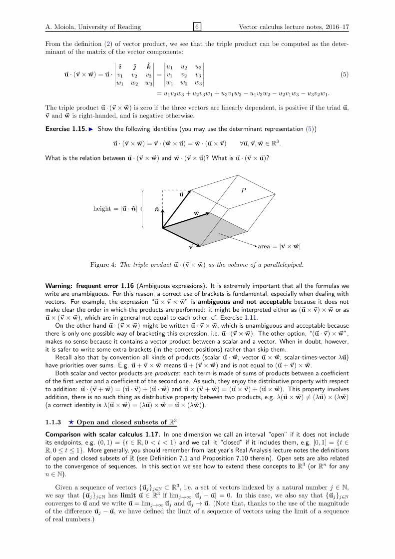
Given three vectors ~u and ~v and ~w, their triple product is the scalar
~u · (~v × ~w).
Its absolute value is the volume of the parallelepiped P defined by the three vectors as in Figure 4. Tosee this, we define the unit vector orthogonal to the plane containing ~v and ~w as n := ~v×~w
|~v×~w| . Then
Volume (P ) : = (area of base) × height = |~v × ~w| |~u · n| = |~v × ~w|∣∣∣∣~u · ~v × ~w
|~v × ~w|
∣∣∣∣ = |~u · (~v × ~w)| .
A. Moiola, University of Reading 6 Vector calculus lecture notes, 2016–17
From the definition (2) of vector product, we see that the triple product can be computed as the deter-minant of the matrix of the vector components:
~u · (~v × ~w) = ~u ·
∣∣∣∣∣∣
ı k
v1 v2 v3w1 w2 w3
∣∣∣∣∣∣=
∣∣∣∣∣∣
u1 u2 u3v1 v2 v3w1 w2 w3
∣∣∣∣∣∣(5)
= u1v2w3 + u2v3w1 + u3v1w2 − u1v3w2 − u2v1w3 − u3v2w1.
The triple product ~u · (~v× ~w) is zero if the three vectors are linearly dependent, is positive if the triad ~u,~v and ~w is right-handed, and is negative otherwise.
Exercise 1.15. Show the following identities (you may use the determinant representation (5))
~u · (~v × ~w) = ~v · (~w × ~u) = ~w · (~u× ~v) ∀~u, ~v, ~w ∈ R3.
What is the relation between ~u · (~v × ~w) and ~w · (~v × ~u)? What is ~u · (~v × ~u)?
~v
~w
~u
n
P
area = |~v × ~w|
height = |~u · n|
Figure 4: The triple product ~u · (~v × ~w) as the volume of a parallelepiped.
Warning: frequent error 1.16 (Ambiguous expressions). It is extremely important that all the formulas wewrite are unambiguous. For this reason, a correct use of brackets is fundamental, especially when dealing withvectors. For example, the expression “~u × ~v × ~w” is ambiguous and not acceptable because it does notmake clear the order in which the products are performed: it might be interpreted either as (~u× ~v)× ~w or as~u× (~v × ~w), which are in general not equal to each other; cf. Exercise 1.11.
On the other hand ~u · (~v× ~w) might be written ~u · ~v× ~w, which is unambiguous and acceptable becausethere is only one possible way of bracketing this expression, i.e. ~u · (~v× ~w). The other option, “(~u · ~v)× ~w”,makes no sense because it contains a vector product between a scalar and a vector. When in doubt, however,it is safer to write some extra brackets (in the correct positions) rather than skip them.
Recall also that by convention all kinds of products (scalar ~u · ~w, vector ~u × ~w, scalar-times-vector λ~u)have priorities over sums. E.g. ~u+ ~v × ~w means ~u+ (~v × ~w) and is not equal to (~u+ ~v)× ~w.
Both scalar and vector products are products: each term is made of sums of products between a coefficientof the first vector and a coefficient of the second one. As such, they enjoy the distributive property with respectto addition: ~u · (~v + ~w) = (~u · ~v) + (~u · ~w) and ~u× (~v + ~w) = (~u × ~v) + (~u × ~w). This property involvesaddition, there is no such thing as distributive property between two products, e.g. λ(~u × ~w) 6= (λ~u)× (λ~w)(a correct identity is λ(~u× ~w) = (λ~u)× ~w = ~u× (λ~w)).
1.1.3 ⋆ Open and closed subsets of R3
Comparison with scalar calculus 1.17. In one dimension we call an interval “open” if it does not includeits endpoints, e.g. (0, 1) = t ∈ R, 0 < t < 1 and we call it “closed” if it includes them, e.g. [0, 1] = t ∈R, 0 ≤ t ≤ 1. More generally, you should remember from last year’s Real Analysis lecture notes the definitionsof open and closed subsets of R (see Definition 7.1 and Proposition 7.10 therein). Open sets are also relatedto the convergence of sequences. In this section we see how to extend these concepts to R3 (or Rn for anyn ∈ N).
Given a sequence of vectors ~ujj∈N ⊂ R3, i.e. a set of vectors indexed by a natural number j ∈ N,we say that ~ujj∈N has limit ~u ∈ R3 if limj→∞ |~uj − ~u| = 0. In this case, we also say that ~ujj∈N
converges to ~u and we write ~u = limj→∞ ~uj and ~uj → ~u. (Note that, thanks to the use of the magnitudeof the difference ~uj − ~u, we have defined the limit of a sequence of vectors using the limit of a sequenceof real numbers.)

A. Moiola, University of Reading 7 Vector calculus lecture notes, 2016–17
Exercise 1.18. (i) Given a sequence of vectors ~ujj∈N ⊂ R3 and ~u ∈ R3, prove that limj→∞ ~uj = ~u ∈ R3
if and only if each of the three real sequences of the three components of ~uj converges to the correspondingcomponent of ~u. In formulas, you have to prove that
limj→∞
~uj = ~u ⇐⇒ limj→∞
(~uj)1 = u1, limj→∞
(~uj)2 = u2, limj→∞
(~uj)3 = u3.
(ii) Find a sequence of vectors ~ujj∈N ⊂ R3 and a vector ~u ∈ R3 such that limj→∞ |~uj | − |~u| = 0 but ~uj
does not converge to ~u.
A set D ⊂ R3 is called an open set if for every point ~p ∈ D, there exists ǫ > 0 (depending on ~p) suchthat all points ~q at distance smaller than ǫ from ~p belong to D. In formulas:
D is open if ∀~p ∈ D, ∃ǫ > 0 s.t. ~q ∈ R3, |~q− ~p| < ǫ ⊂ D.
The word domain is used as a synonym of open set (because the domain of definition of scalar and vectorfields, described in the following, is usually chosen to be an open set). A set C ⊂ R3 is called a closed setif for all sequences contained in C and converging to a limit in R3, the limit belongs to C. In formulas:
C is closed if ∀~pjj∈N ⊂ C s.t. limj→∞
~pj = ~p ∈ R3, we have ~p ∈ C.
Examples of open sets are the open unit ball ~r ∈ R3, |~r| < 1, the open unit cube ~r ∈ R3, 0 < x, y, z < 1,the open half space ~r ∈ R3, x > 0. Examples of closed sets are the closed unit ball ~r ∈ R3, |~r| ≤ 1,the closed unit cube ~r ∈ R3, 0 ≤ x, y, z ≤ 1, the closed half space ~r ∈ R3, x ≥ 0, all the planes e.g.~r ∈ R3, x = 0, the lines e.g. ~r ∈ R3, x = y = 0, the sets made by a single points e.g. ~0. Typically,the sets defined using strict inequalities (i.e. > and <) are open, while those defined with non-strictinequalities or equalities (i.e. ≥, ≤ and =) are closed. Closed sets may be “thin”, like planes and lines,while open sets are always “fat”, as they contain little balls around each point. The empty set and R3 arethe only two sets that are simultaneously open and closed.
Analogous definitions can be given for two dimensional sets, i.e. subsets of R2. Two-dimensionaldomains are also called regions.
Exercise 1.19. Prove that the complement of an open set is closed and vice versa. (This is not easy!)
Notation. In the following we will use the letters D,E, . . . to denote three-dimensional open sets, and theletters P,Q,R, S, . . . to denote two-dimensional open sets. S will also be used to name surfaces.
1.2 Scalar fields, vector fields and curves
The fundamental objects of first-year (scalar) calculus are “functions”, in particular real functions ofa real variable, i.e. rules that associate to every number t ∈ R a second number f(t) ∈ R. In thissection we begin the study of three different extensions of this concept to the vector case, i.e. we considerfunctions whose domains, or codomains, or both, are the three-dimensional Euclidean space R3 (or theplane R2), as opposed to the real line R. Fields3 are functions of position, described by the positionvector ~r = xı + y + zk, so their domain is R3 (or a subset of it). Depending on the kind of output,they are called either scalar fields or vector fields. Curves are vector-valued functions of a real variable.In Remark 1.27 we summarise the mapping properties of all these objects. Scalar fields, vector fields andcurves are described in [1] in Sections 12.1, 15.1 and 11.1 respectively.
1.2.1 Scalar fields
A scalar field is a function f : D → R, where the domain D is an open subset of R3. The value of f at thepoint ~r may be written as f(~r) or f(x, y, z). (This is because a scalar field can equivalently be interpretedas a function of one vector variable or as a function of three scalar variables.) Scalar field may also becalled “multivariate functions” or “functions of several variables” (as in the first-year calculus modulus,see handout 5). Some examples of scalar fields are
f(~r) = x2 − y2, g(~r) = xyez, h(~r) = |~r|4.
We will often consider two-dimensional scalar fields, namely functions f : R → R, where now R is adomain in R2, i.e. a region of the plane. Two-dimensional fields may also be thought as three-dimensionalfields that do not depend on the third variable z (i.e. f(x, y, z) = f(x, y) for all z ∈ R).
3Note that the fields that are object of this section have nothing to do with the algebraic definition of fields as abstractsets provided with addition and multiplication (like R, Q or C). The word “field” is commonly used for both meaning andcan be a source of confusion; the use of “scalar field” and “vector field” is unambiguous.

A. Moiola, University of Reading 8 Vector calculus lecture notes, 2016–17
Smooth scalar fields can be graphically represented using level sets, i.e. sets defined by the equationsf(~r)=constant; see the left plot in Figure 5 for an example. The level sets of a two-dimensional field are(planar) level curves and can be easily drawn, while the level sets of a three-dimensional vector field arethe level surfaces, which are harder to visualise. Level curves are also called contour lines or isolines,and level surfaces are called isosurfaces. Note that two level surfaces (or curves) never intersect eachother, since at every point ~r the field f takes only one value, but they might “self-intersect”.
−3−3
−3−3
−2
−2
−2
−2
−2
−2
−1
−1
−1
−1
−1
−1
0
0
0
0
0
0
0
0
1
1
1
1
1
1
2
2
2
2
3
3
3
3
−2 −1.5 −1 −0.5 0 0.5 1 1.5 2−2
−1.5
−1
−0.5
0
0.5
1
1.5
2
x
y
−2
−1
0
1
2
−2
−1
0
1
2
−4
−3
−2
−1
0
1
2
3
4
xy
z
Figure 5: Left: the level set representation of the scalar field f(~r) = x2 − y2. Since f does not dependon the z-component of the position, we can think at it as a two-dimensional field and represent it with thelevel curves corresponding to a section in the xy-plane. Each colour represents the set of points ~r such thatf(~r) is equal to a certain constant, e.g. f(~r) = 0 along the green lines and f(~r) = 2 along the red curves(see the .pdf file of these notes for the coloured version). This plot is obtained with Matlab’s commandcontour.Right: the same field f = x2 − y2 represented as the surface Sf = ~r ∈ R3 s.t. z = f(x, y); seeRemark 1.21. Surfaces can be drawn in Matlab with the commands mesh and surf.
Example 1.20 (Different fields with the same level sets). Consider the level surfaces of the scalar field f(~r) =|~r|2. Every surface corresponds to the set of points that are solutions of the quadratic equation f(~r) = |~r|2 =x2 + y2 + z2 = C for some C ∈ R (C ≥ 0), thus they are the spheres centred at the origin.
Now consider the level surfaces of the scalar field g(~r) = e−|~r|2 . They correspond to the solutions of the
equation e−x2−y2−z2
= C, or (x2 + y2 + z2) = − logC, for some 0 < C ≤ 1. Therefore also in this case theyare the spheres centred at the origin (indeed the two fields are related by the identity g(~r) = e−f(~r)).
We conclude that two different scalar fields may have the same level surfaces, associated with different fieldvalues (see Figure 6).
Comparison with scalar calculus 1.21 (Graph surfaces). A real function of one variable g : R → R is usuallyrepresented with its graph Gg = (x, y) ∈ R2 s.t. y = g(x), which is a subset of the plane. Exactly in thesame way, a two-dimensional scalar field f : R2 → R can be visualised using its graph
Sf =~r = xı + y+ zk ∈ R3, z = f(x, y)
,
which is a surface, i.e. a two-dimensional set lying in R3; see the example in the right plot of Figure 6. (Westudy surfaces more in detail in Section 2.2.4.) The graph of a general three-dimensional scalar field is ahypersurface and we cannot easily visualise as it is a three-dimensional set living in a four-dimensional space.
Exercise: represent the graphs of the two fields defined in Example 1.20 (or their planar section at z = 0).Despite having the same level sets the surfaces representing their graphs are very different from each other.
⋆ Remark 1.22. A scalar field f : D → R, where D is an open set, is continuous at ~r0 ∈ D if for all ǫ > 0there exists δ > 0 such that for all ~r ∈ D with |~r−~r0| < δ then |f(~r)− f(~r0)| < ǫ. The field f is continuousin D if it is continuous at each point of D. Equivalently, f is continuous at ~r0 ∈ D if for all sequences ofpoints ~rjj∈N ⊂ D with limj→∞~rj = ~r0, it follows that limj→∞ f(~rj) = f(~r0). A continuous field is oftencalled “of class C0”.

A. Moiola, University of Reading 9 Vector calculus lecture notes, 2016–17
1
11
2
2
2
2
2
3
3
3
3
3
34
4
4
4
4
4
5
5
5
5
6
6
6
6
7
7
7
7
−2 −1 0 1 2−2
−1.5
−1
−0.5
0
0.5
1
1.5
2
0.1
0.1
0.1
0.1
0.1
0.2
0.2
0.2
0.2
0.3
0.3
0.3
0.3
0.4
0.4
0.4
0.5
0.5
0.5
0.6
0.6
0.7
0.7
0.8
0.8 0
.9
−2 −1 0 1 2−2
−1.5
−1
−0.5
0
0.5
1
1.5
2
xx
yy
Figure 6: The level sets of the two scalar fields described in Example 1.20; only the plane z = 0 isrepresented here. In the left plot, the field f(~r) = |~r|2 (level sets for the values 1, 2,. . . , 7); in the right
plot, the field g(~r) = e−|~r|2 (level sets for the values 0.1, 0.2,. . . , 0.9). Each level set of f is also a levelset of g (do not forget that the plots represent only few level sets).
Note that studying the continuity of a field can be much more tricky than for a real function. For example,it is clear that the field 1/|~r| is discontinuous at the origin, 1/xyz is discontinuous on the three coordinateplanes and sign(sinx)ey has jump discontinuities on the planes x = πn, n ∈ N. However, in other cases the
discontinuity is somewhat hidden: can you see why the two-dimensional fields f(~r) = 2xyx2+y2 and g(~r) = 2x2y
x4+y2
are both discontinuous at the origin? (You may learn more on this in the “analysis in several variables” module;if you cannot wait take a look at Chapter 12 of [1].)
⋆ Remark 1.23 (Admissible smoothness of fields). In this notes we always assume that scalar and vectorfields we use are “smooth enough” to be able to take all the derivatives we need. We will never be very preciseon this important point, and you can safely ignore it for this module (only!). When we require a field to be“smooth”, we usually mean that it is described by a C∞ function, i.e. that it is continuous and all its partialderivatives (of any order) are continuous. However, in most cases C2 regularity will be enough for our purposes(i.e. we need the continuity of the field and its derivatives up to second order only). For example, wheneverwe write an identity involving the derivatives of a scalar field f , we will be able to consider f(~r) = |~r|2, whichenjoys C∞ regularity, but not f(~r) = |~r| whose partial derivatives are not well-defined at the origin (it is notcontinuously differentiable, i.e. it is not of class C1). See also Remarks 1.22, 1.31 and 1.42 for the definitionof the regularity classes Ck.
1.2.2 Vector fields
A vector field ~F is a function of position whose output is a vector, namely it is a function
~F : D → R3, ~F(~r) = F1(~r) ı+ F2(~r) + F3(~r) k,
where the domain D is a subset of R3. The three scalar fields F1, F2 and F3 are the components of ~F.Some examples of vector fields are
~F(~r) = 2xı− 2y, ~G(~r) = yzı+ xz+ xyk, ~H(~r) = |~r|2ı+ cos y k.
Figure 7 shows two common graphical representations of vector fields.Two-dimensional (or planar) vector fields are functions ~F : R → R2, with R a region in R2. Two-
dimensional vector fields may also be considered as three-dimensional fields that do not depend on thethird variable z, and whose third component ~F3 is identically zero, i.e. ~F(~r) = F1(x, y)ı + F2(x, y). Thefield depicted in Figure 7 is two dimensional.
1.2.3 Curves
Curves are vector-valued functions of a real variable ~a : I → R3, where I is either the real line I = R oran interval I ⊂ R. Since the value ~a(t) at each t ∈ I is a vector, we expand a curve as:
~a(t) = a1(t)ı + a2(t)+ a3(t)k,
A. Moiola, University of Reading 10 Vector calculus lecture notes, 2016–17
−2.5 −2 −1.5 −1 −0.5 0 0.5 1 1.5 2 2.5−2
−1.5
−1
−0.5
0
0.5
1
1.5
2
x
y
−2 −1.5 −1 −0.5 0 0.5 1 1.5 2−2
−1.5
−1
−0.5
0
0.5
1
1.5
2
x
y
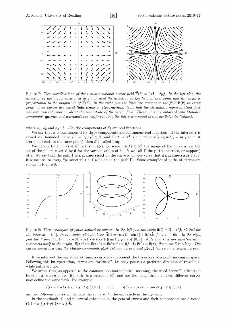
Figure 7: Two visualisations of the two-dimensional vector field ~F(~r) = 2xı − 2y. In the left plot, thedirection of the arrow positioned in ~r indicated the direction of the field in that point and its length isproportional to the magnitude of ~F(~r). In the right plot the lines are tangent to the field ~F(~r) in everypoint; these curves are called field lines or streamlines. Note that the streamline representation doesnot give any information about the magnitude of the vector field. These plots are obtained with Matlab’scommands quiver and streamslice (unfortunately the latter command is not available in Octave).
where a1, a2 and a3 : I → R (the components of ~a) are real functions.We say that ~a is continuous if its three components are continuous real functions. If the interval I is
closed and bounded, namely I = [tI , tF ] ⊂ R, and ~a : I → R3 is a curve satisfying ~a(tI) = ~a(tF ) (i.e. itstarts and ends in the same point), then ~a is called loop.
We denote by Γ := ~r ∈ R3, s.t. ~r = ~a(t), for some t ∈ I ⊂ R3 the image of the curve ~a, i.e. theset of the points covered by ~a for the various values of t ∈ I; we call Γ the path (or trace, or support)of ~a. We say that the path Γ is parametrised by the curve ~a, or vice versa that ~a parametrises Γ (i.e.it associates to every “parameter” t ∈ I a point on the path Γ). Some examples of paths of curves areshown in Figure 8.
−1 −0.5 0 0.5 1−1
−0.8
−0.6
−0.4
−0.2
0
0.2
0.4
0.6
0.8
1
x
y
−1
−0.5
0
0.5
1
−1
−0.5
0
0.5
1
0
0.5
1
1.5
2
xy
z
−1 −0.5 0 0.5 1−1
−0.8
−0.6
−0.4
−0.2
0
0.2
0.4
0.6
0.8
1
x
y
Figure 8: Three examples of paths defined by curves. In the left plot the cubic ~a(t) = tı + t3, plotted for
the interval [−1, 1]. In the centre plot the helix ~b(t) = cos t ı+ sin t + 0.1tk, for t ∈ [0, 6π]. In the rightplot the “clover” ~c(t) = (cos 3t)(cos t)ı + (cos 3t)(sin t) for t ∈ [0, π]. Note that ~c is not injective as itintersects itself in the origin (~c(π/6) = ~c(π/2) = ~c(5π/6) = ~0). As ~c(0) = ~c(π), the curve ~c is a loop. Thecurves are drawn with the Matlab commands plot (planar curves) and plot3 (three-dimensional curves).
If we interpret the variable t as time, a curve may represent the trajectory of a point moving in space.Following this interpretation, curves are “oriented”, i.e. they possess a preferred direction of travelling,while paths are not.
We stress that, as opposed to the common non-mathematical meaning, the word “curve” indicates afunction ~a, whose image (its path) is a subset of R3, and not the image itself. Indeed, different curvesmay define the same path. For example
~a(t) = cos t ı+ sin t t ∈ [0, 2π) and ~b(τ) = cos 2τ ı+ sin 2τ τ ∈ [0, π)
are two different curves which have the same path: the unit circle in the xy-plane.In the textbook [1] and in several other books, the general curves and their components are denoted
~r(t) = x(t)ı + y(t)+ z(t)k.

A. Moiola, University of Reading 11 Vector calculus lecture notes, 2016–17
Remark 1.24 (How to parametrise a path). Given a path (or a curve), how can we find its curve (or its path)?In one direction the procedure is straightforward. If we have the analytic expression of a curve ~a : I → R3,
its path can be drawn (approximately) simply by evaluating ~a(tj) for many tj ∈ I and “connecting the points”.This is exactly what is done automatically by Matlab or Octave to make e.g. Figure 8.
The opposite operation is sometimes very difficult: since every path corresponds to infinitely many curves,there is no universal procedure to construct ~a from Γ. Here we only consider a few simple, but very important,examples. Try to draw all the paths by computing some points via the parametrisation.
• Γ is the segment with vertices ~p and ~q. A parametrisation of Γ is
~a(t) = ~p+ t(~q− ~p) = (1− t)~p+ t~q, for t ∈ [0, 1].
(The components are a1(t) = (1− t)p1 + tq1, a2(t) = (1− t)p2 + tq2 and a3(t) = (1− t)p3 + tq3.)
• Γ is part of the graph of a real function g : I → R laying in the xy-plane (where I ⊂ R is an interval).Then we can take ~a(t) = tı+g(t), for t ∈ I. (The components are a1(t) = t, a2(t) = g(t) and a3(t) = 0.)
• Γ is the circumference with centre ~p = p1ı + p2 and radius R lying in the xy-plane. Then we can take~a(t) = ~p+R cos tı+R sin t for t ∈ [0, 2π). Indeed, this circumference has equation Γ = ~r, (x− p1)
2 +(y − p2)
2 = R2, z = 0, which is satisfied by the curve above (verify this).
• What can we do if the path is defined by an equation? This might require some guesswork. For example,consider the planar ellipse Γ = ~r, x2/9 + y2/4 = 1, z = 0. Since it lies in the plane z = 0, we fixa3(t) = 0 and we look for a1(t) and a2(t). This must be functions of t that satisfy a1(t)
2/9+a2(t)2/4 = 1.
Since the ellipse is an affine deformation of the unit circumference, we may expect to use trigonometricfunctions, and indeed we see that ~a(t) = 3 cos tı+ 2 sin t satisfies the desired equation.
Try to understand well these simple examples (segments, graphs, circumferences): they will be used very oftenduring the course and the solution of many exercises will require their use.
Remark 1.25 (How to change parametrisation). Sometimes we have a curve ~a : I → R3, and we want to
find a different curve ~b : J → R3 with the same path Γ, but defined on a different interval J ⊂ R. To thispurpose, it is enough to find a function g : J → I that is bijective and continuous and define ~b(τ) := ~a(g(τ))
for τ ∈ J . Two parametrisations ~a and ~b of the same path are always related one another by a function g ofthis kind. If g is increasing, then the two parametrisations have the same orientation (they run the path in thesame direction); if g is decreasing, then the two parametrisations have the opposite orientation (they run thepath in opposite directions). We see a few examples.
• In the example above, the unit circle is parametrised by ~a(t) = cos t ı + sin t for t ∈ I = [0, 2π) and~b(τ) = cos 2τ ı+ sin 2τ for τ ∈ J = [0, π), so we have g(τ) = 2τ .
• Consider the unit half circle centred at the origin and located in the half plane ~r = xı+ y, y ≥ 0, whichcan be defined by either of the two parametrisations
~a : [0, π] → R3, ~a(t) = cos tı+ sin t, ~b : [−1, 1] → R3, ~b(τ) = τ ı +√1− τ2.
Here we use g = arccos : [−1, 1] → [0, π] (which is decreasing: ~a runs anti-clockwise, ~b clockwise).
• We can use a change of parametrisation to invert the orientation of a curve. If ~a is defined on the intervalI = [0, tF ], choosing g(τ) = tF − τ we obtain ~b(τ) = ~a(tF − τ) which maps I → Γ (as ~a does) but withopposite orientation.
In the special case of a segment, from ~a(t) = ~p + t(~q − ~p) = (1 − t)~p + t~q for t ∈ [0, 1] we obtain~b(τ) = ~q+ τ(~p− ~q) = τ~p + (1− τ)~q for τ ∈ [0, 1]. ~a runs from ~p to ~q, while ~b runs from ~q to ~p.
⋆ Remark 1.26 (Fields in physics). Fields are important in all branches of science and model many physical
quantities. For example, consider a domain D that models a portion of Earth’s atmosphere. One canassociate to every point ~r ∈ D several numerical quantities representing temperature, density, air pressure,concentration of water vapour or some pollutant (at a given instant): each of these physical quantities canbe mathematically represented by a scalar field (a scalar quantity is associated to each point in space). Otherphysical quantities involve magnitude and direction (which can both vary in different points in space), thus theycan be represented as vector fields: for example the gravitational force, the wind velocity, the magnetic field(pointing to the magnetic north pole). The plots you commonly see in weather forecast are representations ofsome of these fields (e.g. level sets of pressure at a given altitude). (Note that all these fields may vary in time,so they are actually functions of four scalar variables: three spacial and one temporal.) Also curves are used inphysics, for instance to describe trajectories of electrons, bullets, aircraft, planets and any other kind of body.

A. Moiola, University of Reading 12 Vector calculus lecture notes, 2016–17
Warning: frequent error 1.27. At this point it is extremely important not to mix up the different definitionsof scalar fields, vector fields and curves. Treating vectors as scalars or scalars as vectors is one of the
main sources of mistakes in vector calculus exams! We recall that scalar fields take as input a vectorand return a real number (~r 7→ f(~r)), vector fields take as input a vector and return a vector (~r 7→ ~F(~r)),curves take as input a real number and return a vector (t 7→ ~a(t)):
Real functions (of real variable) f : R → R t 7→ f(t),Curves ~a : R → R3 t 7→ ~a(t),Scalar fields f : R3 → R ~r 7→ f(~r),
Vector fields ~F : R3 → R3 ~r 7→ ~F(~r).
Increasing complexity
Vector fields might be thought as combinations of three scalar fields (the components) and curves as com-binations of three real functions.
1.3 Vector differential operators
We learned in the calculus class what is the derivative of a smooth real function of one variable f : R → R.We now study the derivatives of scalar and vector fields. It turns out that there are several important“differential operators”, which generalise the concept of derivative. In this section we introduce them,while in the next one we study some relations between them. The fundamental differential operators forfields are the partial derivatives, described in Section 1.3.1; all the vector differential operators describedin the rest of this section are defined starting from them.
As before, for simplicity we consider here the three-dimensional case only; all the operators, with therelevant exception of the curl operator, can immediately be defined in Rn for any dimension n ∈ N.
The textbook [1] describes partial derivatives in Sections 12.3–5, the Jacobian matrix in 12.6, thegradient and directional derivatives in 12.7, divergence and curl operator in 16.1 and the Laplacian in 16.2.
⋆ Remark 1.28 (What is an operator?). An operator is anything that operates on functions or fields, i.e.a “function of functions” or “function of fields”. For example, we can define the “doubling operator” Tthat, given a real function f : R → R, returns its double, i.e. Tf is the function Tf : R → R, such thatTf(x) = 2f(x).
A differential operator is an operator that involves some differentiation. For example, the derivative ddx
maps f : R → R in ddxf = f ′ : R → R.
Operators and differential operators are rigorously defined using the concept of “function space”, which isan infinite-dimensional vector space whose elements are functions. This is well beyond the scope of this classand is one of the topics studied by functional analysis.
1.3.1 Partial derivatives
Consider a smooth scalar field f : D → R. The partial derivatives of f in the point ~r = xı+y+zk ∈ Dare defined as limits of difference quotients, when these limits exist:
∂f
∂x(~r) := lim
h→0
f(x+ h, y, z)− f(x, y, z)
h,
∂f
∂y(~r) := lim
h→0
f(x, y + h, z)− f(x, y, z)
h, (6)
∂f
∂z(~r) := lim
h→0
f(x, y, z + h)− f(x, y, z)
h.
In other words, ∂f∂x (~r) can be understood as the derivative of the real function x 7→ f(x, y, z) which “freezes”
the y- and z-variables. If the partial derivatives are defined for all points in D, then they constitute threescalar fields, denoted by ∂f
∂x ,∂f∂y and ∂f
∂z . We can also write
∂f
∂x(~r) = lim
h→0
f(~r+ hı)− f(~r)
h,
∂f
∂y(~r) = lim
h→0
f(~r+ h)− f(~r)
h,
∂f
∂z(~r) = lim
h→0
f(~r+ hk)− f(~r)
h.
We also use the notation ∂~F∂x := ∂F1
∂x ı + ∂F2
∂x + ∂F3
∂x k to denote the vector field whose components are
the partial derivatives with respect to x of the components of a vector field ~F (and similarly ∂~F∂y and ∂~F
∂z ).
Exercise 1.29. Compute all the partial derivatives of the following scalar fields:
f(~r) = xyez , g(~r) =xy
y + z, h(~r) = log(1 + z2eyz), ℓ(~r) =
√x2 + y4 + z6, m(~r) = xy , p(~r)=
|~r|2x2
.

A. Moiola, University of Reading 13 Vector calculus lecture notes, 2016–17
Since partial derivative are nothing else than usual derivatives for the functions obtained by freezingall variables except one, the usual rules for derivatives apply. For f and g scalar fields, λ and µ ∈ R, anda real function G : R → R, we have the following identities: linearity
∂(λf + µg)
∂x= λ
∂f
∂x+ µ
∂g
∂x,
∂(λf + µg)
∂y= λ
∂f
∂y+ µ
∂g
∂y,
∂(λf + µg)
∂z= λ
∂f
∂z+ µ
∂g
∂z; (7)
the product rule (extending the well-known formula (FG)′ = F ′G+ FG′ for real functions)
∂(fg)
∂x= g
∂f
∂x+ f
∂g
∂x,
∂(fg)
∂y= g
∂f
∂y+ f
∂g
∂y,
∂(fg)
∂z= g
∂f
∂z+ f
∂g
∂z; (8)
and the chain rule
∂(G(f)
)
∂x= G′(f)
∂f
∂x,
∂(G(f)
)
∂y= G′(f)
∂f
∂y,
∂(G(f)
)
∂z= G′(f)
∂f
∂z. (9)
Note that the product rule (8) must be used when we compute a partial derivative of a product ; the chainrule (9) when we compute a partial derivative of a composition.4 In other words, in (8) the two scalarfields f and g are multiplied to each other, in (9) the function G is evaluated in f(~r), which is a scalar:∂(G(f))
∂x (~r) = G′(f(~r))∂f∂x (~r).
⋆ Remark 1.30. Note that to be able to define the partial derivatives of a field f in a point ~r we need to beable to take the limits in (6), so to evaluate f “nearby” ~r. This is possible if f is defined in a open set D, asdefined in Section 1.1.3, which ensures that all its points are completely surrounded by points of the same set.
For example, the “open half space”D = x > 0 is open, while the “closed half space” E = x ≥ 0 is not.If a field f is defined in E, we can not evaluate f(h, y, z) for negative h, so the limit limh→0
f(h,y,z)−f(0,y,z)h
in (6) is not defined and we cannot compute ∂f∂x in all the points y+ zk ∈ E (those with x = 0).
⋆ Remark 1.31. A scalar field f : D → R is called differentiable or “differentiable of class C1” if it iscontinuous (see Remark 1.22) and all its first-order partial derivatives exist and are continuous. A vector fieldis differentiable (of class C1) if its three components are differentiable.
1.3.2 The gradient
Let f be a scalar field. The vector field whose three components are the three partial derivatives of f (inthe usual order) is called gradient of f and denoted by
~∇f(~r) := grad f(~r) := ı∂f
∂x(~r) +
∂f
∂y(~r) + k
∂f
∂z(~r). (10)
The symbol
~∇ := ı∂
∂x+
∂
∂y+ k
∂
∂z(11)
is called “nabla” operator, or “del”, and is usually denoted simply by ∇.Given a smooth scalar field f and a unit vector u, the directional derivative of f in direction u is
defined as the scalar product ∂f∂u (~r) := u · ~∇f(~r). If n is the unit vector orthogonal to a surface, ∂f
∂n := ∂f∂n
is called normal derivative.
Example 1.32. The gradient of f(~r) = x2 − y2 is
~∇f(~r) = ı∂
∂x(x2 − y2) +
∂
∂y(x2 − y2) + k
∂
∂z(x2 − y2) = 2xı− 2y;
thus the vector field in Figure 7 is the gradient of the scalar field depicted in Figure 5.
4 We recall the notion of composition of functions: for any three sets A, B, C, and two functions F : A → B andG : B → C, the composition of G with F is the function (GF ) : A → C obtained by applying F and then G to the obtainedoutput. In formulas: (G F )(x) := G(F (x)) for all x ∈ A. If A = B = C = R (or they are appropriate subsets of R) and Fand G are differentiable, then from basic calculus we know the derivative of the composition: (G F )′(x) = G′(F (x))F ′(x)(this is the most basic example of chain rule).

A. Moiola, University of Reading 14 Vector calculus lecture notes, 2016–17
Proposition 1.33 (Properties of the gradient). Given two smooth scalar fields f, g : D → R, their gradientssatisfy the following properties:
1. for any constant λ, µ ∈ R, the following identity holds (linearity)
~∇(λf + µg) = λ~∇f + µ~∇g; (12)
2. the following identity holds (product rule or Leibniz rule)
~∇(fg) = g~∇f + f ~∇g; (13)
3. for any differentiable real function G : R → R the chain rule holds:
~∇(G f)(~r) = ~∇G(f(~r)
)= G′(f(~r)
)~∇f(~r), (14)
where G′(f(~r)) is the derivative of G evaluated in f(~r) and G f denotes the composition of G with f ;
4. ~∇f(~r) is perpendicular to the level surface of f passing through ~r (i.e. to ~r′ ∈ D s.t. f(~r′) = f(~r));
5. ~∇f(~r) points in the direction of maximal increase of f .
Proof of 1., 2. and 3. We use the definition of the gradient (10), the linearity (7), the product rule (8)and the chain rule for partial derivatives (9):
~∇(λf + µg) = ı∂(λf + µg)
∂x+
∂(λf + µg)
∂y+ k
∂(λf + µg)
∂z
(7)= ıλ
∂f
∂x+ ıµ
∂g
∂x+ λ
∂f
∂y+ µ
∂g
∂y+ kλ
∂f
∂z+ kµ
∂g
∂z= λ~∇f + µ~∇g;
~∇(fg) = ı∂(fg)
∂x+
∂(fg)
∂y+ k
∂(fg)
∂z
(8)= ı
(g∂f
∂x+ f
∂g
∂x
)+
(g∂f
∂y+ f
∂g
∂y
)+ k
(g∂f
∂z+ f
∂g
∂z
)= g~∇f + f ~∇g,
~∇(G f)(~r) = ı∂(G f)∂x
(~r) + ∂(G f)∂y
(~r) + k∂(G f)∂z
(~r)
(9)= ıG′(f(~r)
)∂f∂x
(~r) + G′(f(~r))∂f∂y
(~r) + kG′(f(~r))∂f∂z
(~r) = G′(f(~r))~∇f(~r).
Parts 4. and 5. will be proved in Remarks 1.88 and 1.89.
Exercise 1.34. Write the gradients of the scalar fields in Exercise 1.29.
Exercise 1.35. Verify that the gradients of the “magnitude scalar field” m(~r) = |~r| and of its squares(~r) = |~r|2 satisfy the identities
~∇s(~r) = ~∇(|~r|2) = 2~r, ~∇m(~r) = ~∇(|~r|) = ~r
|~r| ∀~r ∈ R, ~r 6= ~0. (15)
Represent the two gradients as in Figure 7. Can you compute ~∇(|~r|α) for a general α ∈ R?
Comparison with scalar calculus 1.36. We know from first year calculus that we can infer information ona function of real variable from its derivative. Many of the relations between functions and their derivativescarry over to scalar fields and their gradients, we summarise some of them in the following table. (Recall that“affine” is equivalent to “polynomial of degree at most one”.)
F : R → R is a function of real variable: f : R3 → R is a scalar field:
F ′ = 0 ⇐⇒ F is constant (F (t) = λ, ∀t ∈ R), ~∇f = ~0 ⇐⇒ f is constant (f(~r) = λ, ∀~r ∈ R3),
F ′ = λ ⇐⇒ F is affine (F (t) = tλ+ µ), ~∇f = ~u ⇐⇒ f is affine (f(~r) = ~r · ~u+ µ),
F ′ is a polynomial of degree p the components of ~∇f are polynomials of degree p⇐⇒ F is a polynomial of degree p+ 1, ⇐⇒ f is a polynomial of degree p+ 1 in x, y, z,
F ′ > 0 n · ~∇f > 0 ⇐⇒ f is increasing in direction n
⇐⇒ F is increasing (F (s) < F (t), s < t), (f(~r+ hn) > f(~r), h > 0, here n is a unit vector),
t0 is a local maximum/minumum for F ~r0 is a local maximum/minumum for f
⇒ F ′(t0) = 0, ⇒ ~∇f(~r0) = ~0.
A. Moiola, University of Reading 15 Vector calculus lecture notes, 2016–17
−3−3
−3−3
−2
−2
−2
−2
−2
−2
−1
−1
−1
−1
−1
−1
0
0
0
0
0
0
0
0
1
1
1
1
1
1
2
2
2
2
3
3
3
3
−2 −1.5 −1 −0.5 0 0.5 1 1.5 2−2
−1.5
−1
−0.5
0
0.5
1
1.5
2
x
y
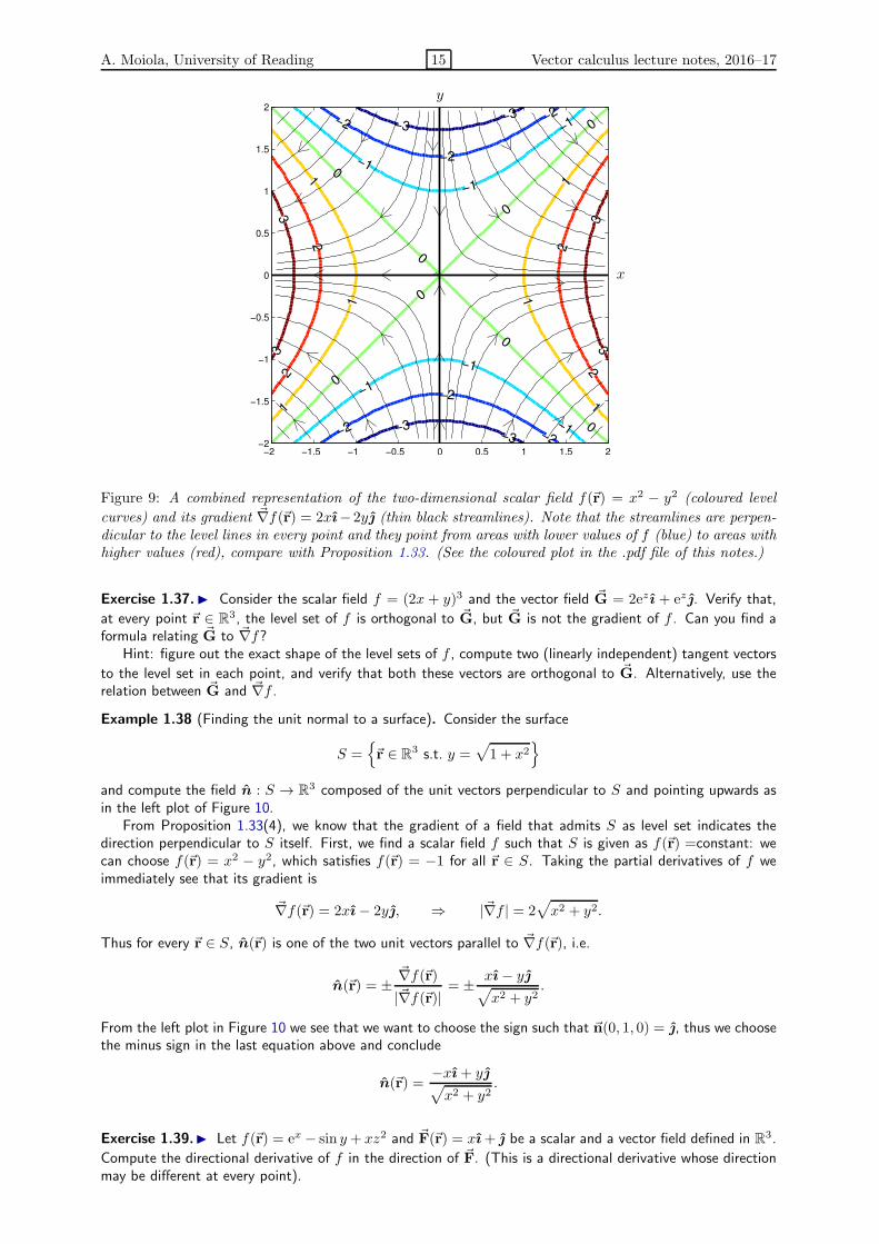
Figure 9: A combined representation of the two-dimensional scalar field f(~r) = x2 − y2 (coloured level
curves) and its gradient ~∇f(~r) = 2xı− 2y (thin black streamlines). Note that the streamlines are perpen-dicular to the level lines in every point and they point from areas with lower values of f (blue) to areas withhigher values (red), compare with Proposition 1.33. (See the coloured plot in the .pdf file of this notes.)
Exercise 1.37. Consider the scalar field f = (2x + y)3 and the vector field ~G = 2ez ı + ez . Verify that,
at every point ~r ∈ R3, the level set of f is orthogonal to ~G, but ~G is not the gradient of f . Can you find aformula relating ~G to ~∇f?
Hint: figure out the exact shape of the level sets of f , compute two (linearly independent) tangent vectors
to the level set in each point, and verify that both these vectors are orthogonal to ~G. Alternatively, use therelation between ~G and ~∇f .Example 1.38 (Finding the unit normal to a surface). Consider the surface
S =~r ∈ R3 s.t. y =
√1 + x2
and compute the field n : S → R3 composed of the unit vectors perpendicular to S and pointing upwards asin the left plot of Figure 10.
From Proposition 1.33(4), we know that the gradient of a field that admits S as level set indicates thedirection perpendicular to S itself. First, we find a scalar field f such that S is given as f(~r) =constant: wecan choose f(~r) = x2 − y2, which satisfies f(~r) = −1 for all ~r ∈ S. Taking the partial derivatives of f weimmediately see that its gradient is
~∇f(~r) = 2xı− 2y, ⇒ |~∇f | = 2√x2 + y2.
Thus for every ~r ∈ S, n(~r) is one of the two unit vectors parallel to ~∇f(~r), i.e.
n(~r) = ±~∇f(~r)|~∇f(~r)|
= ± xı− y√x2 + y2
.
From the left plot in Figure 10 we see that we want to choose the sign such that ~n(0, 1, 0) = , thus we choosethe minus sign in the last equation above and conclude
n(~r) =−xı + y√x2 + y2
.
Exercise 1.39. Let f(~r) = ex − sin y+ xz2 and ~F(~r) = xı+ be a scalar and a vector field defined in R3.
Compute the directional derivative of f in the direction of ~F. (This is a directional derivative whose directionmay be different at every point).

A. Moiola, University of Reading 16 Vector calculus lecture notes, 2016–17
y =√1 + x2
x
y
n
n
n
-1
0
1
2
-2
3
4
5
6
7
8
0 -2-1
01
2 2
Figure 10: Left: The section in the xy-plane (z = 0) of the surface S of Example 1.38 and its unit normalvectors.Right: The surface graph of the planar scalar field f = x2+y2 and its tangent plane at ~r0+f(~r0)k = +k
for ~r0 = . The tangent plane has equation z = f(~r0)+ ~∇f(~r0) · (~r−~r0) = 1+ (2) · (xı+ y− ) = 2y− 1.
⋆ Remark 1.40. The gradient of a scalar field f at a given position ~r0 can be defined as the best linearapproximation of f near ~r0. More precisely, for a differentiable scalar field f : D → R and a point ~r0 ∈ D, thegradient ~∇f(~r0) is the unique vector ~L such that
f(~r) = f(~r0) + ~L · (~r−~r0) + |~r−~r0|g(~r) where lim~r→~r0
g(~r) = 0 and ~r ∈ D.
We know from first-year calculus that, given a differentiable real function F : R → R, the tangent line toits graph at a point (t0, F (t0)) is t 7→ F (t0) + F ′(t0)(t − t0) and the derivative F ′(t0) represents its slope.The tangent line can be defined as the line that best approximates F near t0. Similarly, the affine (i.e. “flat”)
field that best approximates f near ~r0 is ~r 7→ f(~r0) + ~∇f(~r0) · (~r − ~r0). If the field f is two-dimensional,
z = f(~r0) + ~∇f(~r0) · (~r−~r0) is the tangent plane to the surface graph of f (see Remark 1.21), an exampleis in the right plot in Figure 10. If the field is three-dimensional, this is the tangent space to the graph of f ,which now lives in a four-dimensional space, so it is hard to visualise.
1.3.3 The Jacobian matrix
We have seen that a scalar field has three first-order partial derivatives that can be collected in a vectorfield (the gradient). A vector field has nine partial derivatives, three for each component (which is a scalarfield). To represent them compactly we collect them in a matrix.
Consider a smooth vector field ~F, the Jacobian matrix J~F (or simply the Jacobian, named after
Carl Gustav Jacob Jacobi 1804–1851) of ~F is
J~F :=
∂F1
∂x
∂F1
∂y
∂F1
∂z
∂F2
∂x
∂F2
∂y
∂F2
∂z
∂F3
∂x
∂F3
∂y
∂F3
∂z
. (16)
This is a field whose values at each point are 3 × 3 matrices. Note that sometimes the noun “Jacobian”is used to indicate the determinant of the Jacobian matrix.
Exercise 1.41. Compute the Jacobian of the following vector fields
~F(~r) = 2xı− 2y, ~G(~r) = yzı+ xz+ xyk, ~H(~r) = |~r|2ı+ cos yk.
1.3.4 Second-order partial derivatives, the Laplacian and the Hessian
The second-order partial derivatives of a scalar field f are the partial derivatives of the partial derivativesof f . When partial derivatives are taken twice with respect to the same component of the position, they

A. Moiola, University of Reading 17 Vector calculus lecture notes, 2016–17
are denoted by∂2f
∂x2=
∂
∂x
∂f
∂x,
∂2f
∂y2=
∂
∂y
∂f
∂yand
∂2f
∂z2=
∂
∂z
∂f
∂z.
When they are taken with respect to two different components, they are called “mixed derivatives” anddenoted by
∂2f
∂x∂y=
∂
∂x
∂f
∂y,
∂2f
∂x∂z=
∂
∂x
∂f
∂z,
∂2f
∂y∂x=
∂
∂y
∂f
∂x,
∂2f
∂y∂z=
∂
∂y
∂f
∂z,
∂2f
∂z∂x=
∂
∂z
∂f
∂x, and
∂2f
∂z∂y=
∂
∂z
∂f
∂y.
If f is smooth, the order of differentiation is not relevant (Clairault’s or Schwarz theorem):
∂2f
∂x∂y=
∂2f
∂y∂x,
∂2f
∂x∂z=
∂2f
∂z∂xand
∂2f
∂y∂z=
∂2f
∂z∂y. (17)
⋆ Remark 1.42. It is clear that we can define partial derivatives of higher order, e.g. ∂3f∂x2∂y = ∂
∂x∂∂x
∂f∂y . A
scalar field f : D → R is called “differentiable of class Ck” with k ∈ N, if it is continuous (see Remark 1.22),all its partial derivatives of order up to k exist and are continuous. It is called “differentiable of class C∞” ifall its partial derivatives of any order exist and are continuous.
The Laplacian ∆f (or Laplace operator, sometimes denoted by ∇2f , named after Pierre-SimonLaplace 1749–1827)5 of a smooth scalar field f is the scalar field obtained as sum of the pure secondpartial derivatives of f :
∆f := ∇2f :=∂2f
∂x2+∂2f
∂y2+∂2f
∂z2. (18)
A scalar field whose Laplacian vanishes everywhere is called harmonic function.
⋆ Remark 1.43 (Applications of the Laplacian). The Laplacian is used in some of the most studied partialdifferential equations (PDEs) such as the Poisson equation∆u = f and the Helmholtz equation−∆u−k2u = f .Therefore, it is ubiquitous and extremely important in physics and engineering, e.g. in the models of diffusionof heat or fluids, electromagnetism, acoustics, wave propagation, quantum mechanics. In the words of T. Tao6:“The Laplacian of a function u at a point x measures the average extent to which the value of u at x deviatesfrom the value of u at nearby points to x (cf. the mean value theorem for harmonic functions). As such, itnaturally occurs in any system in which some quantity at a point is influenced by the value of the same quantityat nearby points.”
The Hessian Hf (or Hessian matrix, named after Ludwig Otto Hesse 1811–1874) is the 3× 3 matrixfield of the second derivatives of the scalar field f :
Hf := J(~∇f) =
∂2f
∂x2∂2f
∂y∂x
∂2f
∂z∂x
∂2f
∂x∂y
∂2f
∂y2∂2f
∂z∂y
∂2f
∂x∂z
∂2f
∂y∂z
∂2f
∂z2
. (19)
Note that, thanks to Clairault’s theorem (17), (if the field f is smooth enough) the Hessian is a symmetricmatrix in every point. The Laplacian equals the trace of the Hessian, i.e. the sum of its diagonal terms:
∆f = Tr(Hf). (20)
The vector Laplacian ~∆ is the Laplace operator applied componentwise to vector fields:
~∆~F := (∆F1 )ı + (∆F2)+ (∆F3)k (21)
=(∂2F1
∂x2+∂2F1
∂y2+∂2F1
∂z2
)ı+
(∂2F2
∂x2+∂2F2
∂y2+∂2F2
∂z2
)+
(∂2F3
∂x2+∂2F3
∂y2+∂2F3
∂z2
)k.
5The reason for the use of the notation ∇2 will be slightly more clear after equation (24); this symbol is mainly used byphysicists and engineers.
6http://mathoverflow.net/questions/54986

A. Moiola, University of Reading 18 Vector calculus lecture notes, 2016–17
Exercise 1.44. Compute the Laplacian and the Hessian of the following scalar fields:
f(~r) = x2 − y2, g(~r) = xyez, h(~r) = |~r|4.
Warning: frequent error 1.45. Once again, we remind that symbols cannot be moved around freely in
mathematical expressions. For example, ∂f∂x
∂g∂y ,
∂f∂y
∂g∂x ,
∂2(fg)∂x∂y and g ∂2f
∂x∂y , are all different fields and must not
be confused with each other. Equation (17) only says that we can swap the order of derivation for the same
field, not between two fields, i.e. ∂2f∂x∂y = ∂2f
∂y∂x but ∂f∂x
∂g∂y 6= ∂f
∂y∂g∂x . Moreover ∂fg
∂x does not mean anything: is
it supposed to be ∂(fg)∂x or (∂f∂x )g? All these errors appears too often in exams, watch out!
1.3.5 The divergence operator
Given a differentiable vector field ~F, its divergence is defined as the the trace of its Jacobian matrix:
~∇ · ~F := div ~F := Tr(J~F) =∂F1
∂x+∂F2
∂y+∂F3
∂z. (22)
The notation ~∇· ~F is justified by the fact that the divergence can be written as the formal scalar productbetween the nabla symbol ~∇ and the field ~F:
~∇ · ~F =(ı∂
∂x+
∂
∂y+ k
∂
∂z
)·(F1ı + F2+ F3k
).
Exercise 1.46. Compute the divergence of the following vector fields:
~F(~r) = 2xı− 2y, ~G(~r) = yzı+ xz+ xyk, ~H(~r) = |~r|2ı+ cos yk.
What is the intuitive meaning of the divergence of a vector field ~F? Very roughly speaking, thedivergence measures the “spreading” of ~F around a point ~r, i.e. the difference between the amount of ~Fexiting from an infinitesimally small ball centred at ~r and the amount entering it. If ~∇ · ~F is positivein ~r we may expect ~F to spread or expand near ~r, while if it is negative ~F will shrink. Of course thisis explanation is extremely hand-waving: we will prove a precise characterisation of the meaning of thedivergence in Remark 3.33.
Example 1.47 (Positive and negative divergence). The field ~F = xı + y has positive divergence ~∇ · ~F =1 + 1 + 0 = 2 > 0, thus we see in the left plot of Figure 11 that it is somewhat spreading. The field~G = (−x − 2y)ı + (2x − y) has negative divergence ~∇ · ~G = −1 − 1 + 0 = −2 < 0, and we see from theright plot that the field is converging.
−2.5 −2 −1.5 −1 −0.5 0 0.5 1 1.5 2 2.5
−2
−1.5
−1
−0.5
0
0.5
1
1.5
2
−2.5 −2 −1.5 −1 −0.5 0 0.5 1 1.5 2 2.5
−2
−1.5
−1
−0.5
0
0.5
1
1.5
2
Figure 11: A representation of the fields ~F = xı + y (left) and ~G = (−x− 2y)ı+ (2x− y) (right) from
Example 1.47. ~F has positive divergence and ~G negative.
⋆ Remark 1.48. From the previous example it seems to be possible to deduce the sign of the divergenceof a vector field from its plot, observing whether the arrows “converge” or “diverge”. However, this can bemisleading, as also the magnitude (the length of the arrows) matters. For example, the fields ~Fa = |~r|−a~rdefined in R3 \ ~0, where a is a real positive parameter, have similar plots but they have positive divergenceif a < 3 and negative if a > 3. (Can you show this fact? It is not easy!)

A. Moiola, University of Reading 19 Vector calculus lecture notes, 2016–17
−0.5 0 0.5 1 1.5
−0.4
−0.2
0
0.2
0.4
0.6
0.8
1
1.2
1.4
1.6
Figure 12: The field ~F = (x2 − x)ı+ (y2 − y) has divergence ~∇ · ~F = 2(x+ y− 1) which is positive above
the straight line x+ y = 1 and negative below. If ~F represents the velocity of a fluid, the upper part of thespace acts like a source and the lower part as a sink.
Warning: frequent error 1.49. Since strictly speaking ~∇ is not a vector (11), the symbol ~∇ · ~F does notrepresent a scalar product and7
~∇ · ~F 6= ~F · ~∇.Recall: you can not move around the nabla symbol ~∇ in a mathematical expression!
1.3.6 The curl operator
The last differential operator we define is the curl operator ~∇× (often denoted “curl” and more rarely“rot” and called rotor or rotational), which maps vector fields to vector fields:
~∇× ~F := curl ~F : =
∣∣∣∣∣∣
ı k∂∂x
∂∂y
∂∂z
F1 F2 F3
∣∣∣∣∣∣=(∂F3
∂y− ∂F2
∂z
)ı+
(∂F1
∂z− ∂F3
∂x
)+
(∂F2
∂x− ∂F1
∂y
)k. (23)
As in the definition of the vector product (2), the matrix determinant is purely formal, since it contains
vectors, differential operators and scalar fields. Again, ~∇× ~F 6= −~F× ~∇, as the left-hand side is a vectorfield while the right-hand side is a differential operator.
Among all the differential operators introduced so far, the curl operator is the only one which can bedefined only in three dimensions, since it is related to the vector product.
Exercise 1.50. Compute the curl of the following vector fields:
~F(~r) = 2xı− 2y, ~G(~r) = yzı+ xz+ xyk, ~H(~r) = |~r|2ı+ cos yk.
How can we interpret the curl of a field? The curl is in some way a measure of the “rotation” of thefield. If we imagine to place a microscopic paddle-wheel at a point ~r in a fluid moving with velocity ~F,it will rotate with angular velocity proportional to |~∇× ~F(~r)| and rotation axis parallel to ~∇× ~F(~r). Ifthe fluid motion is planar, i.e. F3 = 0, and anti-clockwise, the curl will point out of page, if the motion isclockwise it will point into the page (as the motion of a usual screw). See also Figure 13.
7 Indeed ~∇ · ~F and ~F · ~∇ are two very different mathematical objects: ~∇ · ~F is a scalar field, while ~F · ~∇ is an operatorthat maps scalar fields to scalar fields
(~F · ~∇)f =(F1
∂
∂x+ F2
∂
∂y+ F3
∂
∂z
)f = F1
∂f
∂x+ F2
∂f
∂y+ F3
∂f
∂z.
For example if ~G = yzı+ xz+ xyk and g = xyez , then
(~G · ~∇)g =(yz
∂
∂x+ xz
∂
∂y+ xy
∂
∂z
)g = yz yez + xz xez + xy xyez = (x2z + y2z + x2y2)ez .
The operator ~F · ~∇ can also be applied componentwise to a vector field (and in this case it returns a vector field, see (35)).~F · ~∇ is often called advection operator; when |~F| = 1, then it corresponds to the directional derivative we have alreadyencountered in Section 1.3.2. We will use the advection operator only in Remark 1.56; in any other situation in this moduleyou should not use the symbol (~F · ~∇).

A. Moiola, University of Reading 20 Vector calculus lecture notes, 2016–17
−2.5 −2 −1.5 −1 −0.5 0 0.5 1 1.5 2 2.5
−2
−1.5
−1
−0.5
0
0.5
1
1.5
2
−2.5 −2 −1.5 −1 −0.5 0 0.5 1 1.5 2 2.5−2
−1.5
−1
−0.5
0
0.5
1
1.5
2
Figure 13: The planar field ~F = 2yı − x depicted in the left plot has curl equal to ~∇ × ~F = −3k which“points into the page”, in agreement with the clockwise rotation of ~F. The planar field ~G = x2 depictedin the right plot has curl equal to ~∇× ~G = 2xk which points “into the page” for x < 0 and “out of thepage” for x > 0. Indeed, if we imagine to immerse some paddle-wheels in the field, due to the differencesin the magnitude of the field on their two sides, they will rotate clockwise in the negative-x half-plane andanti-clockwise in the positive-x half-plane.
⋆ Remark 1.51 (Linearity of differential operators). All operators introduced in this section (partial derivatives,gradient, Jacobian, Laplacian, Hessian, divergence, curl) are linear operators. This means that, denoting D anyof these operators, for all λ, µ ∈ R and for any two suitable fields F and G (either both scalar or both vectorfields, depending on which operator is considered), we have the identity D(λF + µG) = λD(F ) + µD(G).
1.4 Vector differential identities
In the following two propositions we prove several identities involving scalar and vector fields and thedifferential operators defined so far. It is fundamental to apply each operator to a field of the appropriatekind, for example we can not compute the divergence of a scalar field because we have not given anymeaning to this object. For this reason, we summarise in Table 1 which types of fields are taken as inputand returned as output by the various operators.
Operator name symbol field taken as input field returned as output order
Partial derivative ∂∂x ,
∂∂y or ∂
∂z scalar scalar 1st
Gradient ~∇ scalar vector 1st
Jacobian J vector matrix 1st
Laplacian ∆ scalar scalar 2nd
Hessian H scalar matrix 2nd
Vector Laplacian ~∆ vector vector 2nd
Divergence ~∇· (or div) vector scalar 1st
Curl (only 3D) ~∇× (or curl) vector vector 1st
Table 1: A summary of the differential operators defined in Section 1.3. The last column shows the orderof the partial derivatives involved in each operator.
1.4.1 Second-order vector differential identities
Next proposition shows the result of taking the divergence or the curl of gradients and curls.
Proposition 1.52 (Vector differential identities for a single field). Let f be a scalar field and ~F be a vectorfield, both defined in a domain D ⊂ R3. Then the following identities hold true:
~∇ · (~∇f) = ∆f, (24)
~∇ · (~∇× ~F) = 0, (25)
~∇× (~∇f) = ~0, (26)
~∇× (~∇× ~F) = ~∇(~∇ · ~F)− ~∆~F. (27)

A. Moiola, University of Reading 21 Vector calculus lecture notes, 2016–17
Proof. The two scalar identities (24) and (25) can be proved using only the definitions of the differential
operators involved (note that we write (~∇f)1 and (~∇×~F)1 to denote the x-components of the correspondingvector fields, and similarly for y and z):
~∇ · (~∇f) (22)=
∂((~∇f)1
)
∂x+∂((~∇f)2
)
∂y+∂((~∇f)3
)
∂z
(10)=
∂
∂x
∂f
∂x+
∂
∂y
∂f
∂y+
∂
∂z
∂f
∂z(18)= ∆f,
~∇ · (~∇× ~F)(22)=
∂((~∇× ~F)1
)
∂x+∂((~∇× ~F)2
)
∂y+∂((~∇× ~F)3
)
∂z
(23)=
∂(
∂F3
∂y − ∂F2
∂z
)
∂x+∂(
∂F1
∂z − ∂F3
∂x
)
∂y+∂(
∂F2
∂x − ∂F1
∂y
)
∂z
=∂2F1
∂y∂z− ∂2F1
∂z∂y+∂2F2
∂z∂x− ∂2F2
∂x∂z+∂2F3
∂x∂y− ∂2F3
∂y∂x(17)= 0.
An alternative proof of (24) uses the facts that the divergence is the trace of the Jacobian matrix (22),the Jacobian matrix of a gradient is the Hessian (19), and the trace of the Hessian is the Laplacian (20):
~∇ · (~∇f) (22)= Tr(J ~∇f) (19)
= Tr(Hf)(20)= ∆f.
The two remaining vector identities can be proved componentwise, i.e. by showing that each of thethree components of the left-hand side is equal to the corresponding component of the right-hand side:
(~∇× (~∇f)
)1
(23)=
∂((~∇f)3
)
∂y− ∂
((~∇f)2
)
∂z
(10)=
∂
∂y
∂f
∂z− ∂
∂z
∂f
∂y(17)= 0,
(~∇× (~∇× ~F)
)1
(23)=
∂((~∇× ~F)3
)
∂y− ∂
((~∇× ~F)2
)
∂z
(23)=
∂
∂y
(∂F2
∂x− ∂F1
∂y
)− ∂
∂z
(∂F1
∂z− ∂F3
∂x
)
(17)=
∂
∂x
(∂F2
∂y+∂F3
∂z
)− ∂2F1
∂y2− ∂2F1
∂z2
=∂
∂x
(∂F1
∂x+∂F2
∂y+∂F3
∂z
)− ∂2F1
∂x2− ∂2F1
∂y2− ∂2F1
∂z2
(22),(18)=
∂
∂x(~∇ · ~F)−∆F1
(10),(21)=
(~∇(~∇ · ~F)− ~∆~F
)
1,
and similarly for the y- and z-components.
Note that, when we prove a certain vector identity, even if we consider only the first component of theequality, this may involve all components of the fields involved and partial derivatives with respect to allvariables ; see for instance the proofs of (26) and (27).
⋆ Remark 1.53. Since in all the identities of Proposition 1.52 we take second derivatives, the precise assump-tions for this proposition are that f and (the components of) ~F are differentiable of class C2.
1.4.2 Vector product rules
Comparison with scalar calculus 1.54. When we compute the derivative of the product of two functions of realvariable we apply the well-known product rule (fg)′ = f ′g+ g′f . When we calculate partial derivatives or thegradient of the product of two scalar fields, similar rules apply, see Equations (8) and (13). But scalar and vectorfields may be multiplied in several different ways (scalar product, vector product and scalar-vector product)

A. Moiola, University of Reading 22 Vector calculus lecture notes, 2016–17
and other differential operators may be applied to these products (divergence, curl, Laplacian,. . . ). In thesecases, the product rules obtained are slightly more complicated; they are described in next Proposition 1.55(and Remark 1.56). Note the common structure of all these identities: a differential operator applied to aproduct of two fields (at the left-hand side) is equal to the sum of some terms containing the derivative of thefirst field only and some terms containing derivatives of the second field only (at the right-hand side).
A special identity is (32): since the Laplacian contains second-order partial derivatives, all terms at theright-hand side contain two derivatives, exactly as in the 1D product rule for second derivatives (fg)′′ =f ′′g + 2f ′g′ + fg′′.
Proposition 1.55 (Vector differential identities for two fields, product rules for differential operators).
Let f and g be scalar fields, ~F and ~G be vector fields, all of them defined in the same domain D ⊂ R3. Thenthe following identities hold true8:
~∇(fg) = f ~∇g + g~∇f, (28)
~∇ · (f ~G) = (~∇f) · ~G+ f ~∇ · ~G, (29)
~∇ · (~F× ~G) = (~∇× ~F) · ~G− ~F · (~∇× ~G), (30)
~∇× (f ~G) = (~∇f)× ~G+ f ~∇× ~G, (31)
∆(fg) = (∆f)g + 2~∇f · ~∇g + f(∆g). (32)
Proof. Identity (28) has already been proven in Proposition 1.33. We show here the proof of identities(30) and (32) only; identities (29) and (31) can be proven with a similar technique. All the proofs use onlythe definitions of the differential operators and of the vector operations (scalar and vector product), theproduct rule (8) for partial derivatives, together with some smart rearrangements of the terms. In somecases, it is convenient to start the proof from the expression at the right-hand side, or even to expandboth sides and match the results obtained. The vector identity (31) is proven componentwise (see thesimilar proof of (33) below).
Identity (30) can be proved as follows:
~∇ · (~F× ~G)(22)=
∂((~F× ~G)1
)
∂x+∂((~F× ~G)2
)
∂y+∂((~F× ~G)3
)
∂z
(2)=∂(F2G3 − F3G2
)
∂x+∂(F3G1 − F1G3
)
∂y+∂(F1G2 − F2G1
)
∂z
(8)=∂F2
∂xG3 + F2
∂G3
∂x− ∂F3
∂xG2 − F3
∂G2
∂x+∂F3
∂yG1 + F3
∂G1
∂y− ∂F1
∂yG3 − F1
∂G3
∂y
+∂F1
∂zG2 + F1
∂G2
∂z− ∂F2
∂zG1 − F2
∂G1
∂z(now collect non-derivative terms)
=
(∂F3
∂y− ∂F2
∂z
)G1 +
(∂F1
∂z− ∂F3
∂x
)G2 +
(∂F2
∂x− ∂F1
∂y
)G3
− F1
(∂G3
∂y− ∂G2
∂z
)− F2
(∂G1
∂z− ∂G3
∂x
)− F3
(∂G2
∂x− ∂G1
∂y
)
(23)= (~∇× ~F)1G1 + (~∇× ~F)2G2 + (~∇× ~F)3G3 − F1(~∇× ~G)1 − F2(~∇× ~G)2 − F3(~∇× ~G)3(1)= (~∇× ~F) · ~G− ~F · (~∇× ~G).
Identity (32) follows from a repeated application of the product rule (8):
∆(fg)(18)=
∂2(fg)
∂x2+∂2(fg)
∂y2+∂2(fg)
∂z2
(8)=
∂
∂x
(∂f
∂xg + f
∂g
∂x
)+
∂
∂y
(∂f
∂yg + f
∂g
∂y
)+
∂
∂z
(∂f
∂zg + f
∂g
∂z
)
(8)=
(∂2f
∂x2g + 2
∂f
∂x
∂g
∂x+ f
∂2g
∂x2
)+
(∂2f
∂y2g + 2
∂f
∂y
∂g
∂y+ f
∂2g
∂y2
)+
(∂2f
∂z2g + 2
∂f
∂z
∂g
∂z+ f
∂2g
∂z2
)
(18),(10),(1)= (∆f)g + 2~∇f · ~∇g + f(∆g).
8You do not need to remember these identities by hearth, even though are simple, but you need to be able to use themand to derive them.⋆ Here the precise assumptions for the proposition are that all fields are differentiable of class C1, except for identity (32)where class C2 is required.

A. Moiola, University of Reading 23 Vector calculus lecture notes, 2016–17
The following is an alternative proof of identity (32) that uses the vector identities previously proved:
∆(fg)(24)= ~∇·
(~∇(fg)
)
(28)= ~∇·(f ~∇g + g~∇f)(12)= ~∇·(f ~∇g) + ~∇·(g~∇f)(29)= (~∇f) · (~∇g) + f ~∇ · (~∇g) + (~∇g) · (~∇f) + g~∇ · (~∇f)(24)= (∆f)g + 2~∇f · ~∇g + f(∆g).
⋆ Remark 1.56. In Proposition 1.55 we found expression (28) for the gradient of the product of two scalarfields. What about the gradient of the scalar product of two vector fields? We also computed the divergence(29) and the curl (31) of the product of a vector and a scalar field, and the divergence of the vector productbetween two vector fields (30). What about the curl of a vector product? The answer two these two questionsis given by the following two vector product rules:
~∇(~F · ~G) = (~F · ~∇)~G+ (~G · ~∇)~F+ ~G× (~∇× ~F) + ~F× (~∇× ~G), (33)
~∇× (~F× ~G) = (~∇ · ~G)~F− (~∇ · ~F)~G+ (~G · ~∇)~F− (~F · ~∇)~G. (34)
In identities (33) and (34) we use the advection operator (which was mentioned in Remark 1.49) applied toa vector field:
(~G · ~∇)~F = (~G · ~∇)F1 ı+ (~G · ~∇)F2+ (~G · ~∇)F3k (35)
=(G1
∂F1
∂x+G2
∂F1
∂y+G3
∂F1
∂z
)ı +
(G1
∂F2
∂x+G2
∂F2
∂y+G3
∂F2
∂z
)+
(G1
∂F3
∂x+G2
∂F3
∂y+G3
∂F3
∂z
)k.
Proof of (33). We prove (33) componentwise, starting from the first component of the expression at theright-hand side:((~F · ~∇)~G+ (~G · ~∇)~F+ ~G× (~∇× ~F) + ~F× (~∇× ~G)
)
1
(2)= (~F · ~∇)G1 + (~G · ~∇)F1 +G2(~∇× ~F)3 −G3(~∇× ~F)2 + F2(~∇× ~G)3 − F3(~∇× ~G)2
(23)=
(F1∂G1
∂x+ F2
∂G1
∂y+ F3
∂G1
∂z
)+
(G1
∂F1
∂x+G2
∂F1
∂y+G3
∂F1
∂z
)
+G2
(∂F2
∂x− ∂F1
∂y
)−G3
(∂F1
∂z− ∂F3
∂x
)+ F2
(∂G2
∂x− ∂G1
∂y
)− F3
(∂G1
∂z− ∂G3
∂x
)
(collect the six non-derivative terms F1, F2,. . . )
= F1∂G1
∂x+ F2
∂G2
∂x+ F3
∂G3
∂x+G1
∂F1
∂x+G2
∂F2
∂x+G3
∂F3
∂x(collect terms pairwise)
=
(F1∂G1
∂x+G1
∂F1
∂x
)+
(F2∂G2
∂x+G2
∂F2
∂x
)+
(F3∂G3
∂x+G3
∂F3
∂x
)
(8)=∂(F1G1)
∂x+∂(F2G2)
∂x+∂(F3G3)
∂x
(1)=∂(~F · ~G)
∂x(10)=(~∇(~F · ~G)
)1,
and similarly for the y- and z-components.
Exercise 1.57. Prove identities (29), (31) and (34) .
Remark 1.58 (Why use vector identities?). Despite looking complicated at a first glance, the identities pre-sented in this section are very useful tools to simplify computations involving differential operators. If you learnhow to use them—rather than reinventing the wheel each time expanding all expressions in components andthe operators in partial derivatives—many exercises and theoretical results in the rest of this module and infuture courses will definitely turn out easier.
Consider, for example the following exercise, which was part of the exam in May 2014.
Let f and g be two smooth scalar fields. Prove the following identity: ~∇× (f ~∇g) + ~∇× (g~∇f) = ~0.

A. Moiola, University of Reading 24 Vector calculus lecture notes, 2016–17
Using two vector identities and the linearity of curl, the solution takes no more than one line9:
~∇× (f ~∇g) + ~∇× (g~∇f) = ~∇× (f ~∇g + g~∇f) (28)= ~∇×
(~∇(fg)
) (26)= ~0.
If you do not use the vector identities as above, but prove the result componentwise, the solution is longer anddefinitely much more subject to mistakes: for the first component we have
(~∇× (f ~∇g) + ~∇× (g~∇f)
)1
(23)=
∂
∂y(f ~∇g)3 −
∂
∂z(f ~∇g)2 +
∂
∂y(g~∇f)3 −
∂
∂z(g~∇f)2
(10)=
∂
∂y
(f∂g
∂z
)− ∂
∂z
(f∂g
∂y
)+
∂
∂y
(g∂f
∂z
)− ∂
∂z
(g∂f
∂y
)
(8)=∂f
∂y
∂g
∂z+ f
∂2g
∂y∂z− ∂f
∂z
∂g
∂y+ f
∂2g
∂z∂y+∂g
∂y
∂f
∂z+ g
∂2f
∂y∂z− ∂g
∂z
∂f
∂y+ g
∂2f
∂z∂y(17)= 0,
and similarly for the second and third components.
⋆ Remark 1.59. As a further example of the convenience of the use of vector notation consider the followingexample. The so-called “Maxwell equations in time-harmonic regime” describe the propagation of an electricfield ~E (a vector field) in a homogeneous materials under certain physical conditions. These partial differentialequations in vector form simply read as:
~∇× (~∇× ~E)− k2~E = ~0,
where k is a positive scalar called wavenumber. The same equations written in coordinates have a morecomplicated and obscure expression (compare with the proof of (27)):
∂2E2
∂x∂y+∂2E3
∂x∂z− ∂2E1
∂y2− ∂2E1
∂z2− k2E1 = 0,
∂2E1
∂x∂y+∂2E3
∂y∂z− ∂2E2
∂x2− ∂2E2
∂z2− k2E2 = 0,
∂2E1
∂x∂z+∂2E2
∂y∂z− ∂2E3
∂x2− ∂2E3
∂y2− k2E3 = 0.
Example 1.60. We demonstrate some of the results of Proposition 1.52 for the vector field~F = xyı + ey cosx + z2k:
~∇ · ~F = y + ey cosx+ 2z,
~∇× ~F = (0− 0)ı+ (0 − 0)+ (ey sinx− x)k = (ey sinx− x)k,
~∇(~∇ · ~F) = −ey sinx ı + (1 + ey cosx) + 2k,
~∇× ~∇× ~F = ey sinxı− (ey cosx− 1),
~∆~F = ∆(xy)ı +∆(ey cosx) +∆(z2)k = 0+ (−ey cosx+ ey cosx)+ 2k = 2k
and from the last three formulas we immediately demonstrate (27). Since ~∇×~F is parallel to k and independentof z, its divergence vanishes, thus also the identity (25) is verified.
Exercise 1.61. Demonstrate identity (30) for the fields ~F = zı+ x2+ y3k and ~G = exyk.
Exercise 1.62. Let α ∈ R be a constant. Prove that (Hint: recall Exercise 1.35.)
~∇ · (|~r|α~r) = (3 + α)|~r|α and ~∇× (|~r|α~r) = ~0.
Exercise 1.63. (i) Prove that ~∇× (f ~∇f) = ~0 for all smooth scalar fields f .
(ii) Prove that, for all natural numbers n, ℓ ∈ N, the more general identity ~∇× (fn~∇(f ℓ)) = ~0 holds true.Here fn and f ℓ simply denote the nth and ℓth powers of f .
Hint: use an appropriate version of the chain rule to compute the gradients of f ℓ and fn.
⋆ Remark 1.64. The following identity involving the Jacobian matrix holds true:
(~∇× ~F)× ~G =(J~F− (J~F)T
)~G,
where the symbol T denotes matrix transposition. Try to prove it for exercise.9Another possible solution using two vector identities and the anti-commutativity of the vector product is the following:
~∇× (f ~∇g) + ~∇× (g~∇f)(31)= (~∇f) × (~∇g) + f ~∇× (~∇g)
︸ ︷︷ ︸=~0, (26)
+(~∇g)× (~∇f) + g ~∇× (~∇f)︸ ︷︷ ︸=~0, (26)
(3)= (~∇f) × (~∇g) − (~∇f) × (~∇g) = ~0.
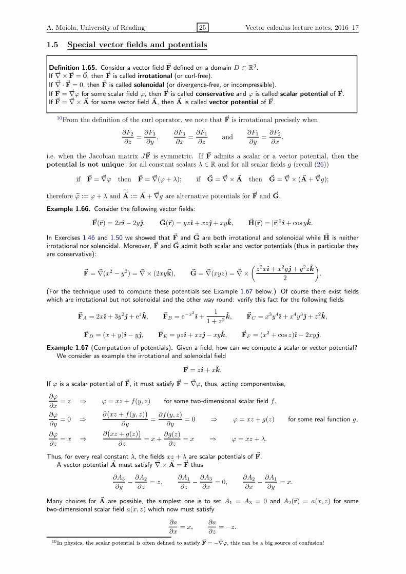
A. Moiola, University of Reading 25 Vector calculus lecture notes, 2016–17
1.5 Special vector fields and potentials
Definition 1.65. Consider a vector field ~F defined on a domain D ⊂ R3.If ~∇× ~F = ~0, then ~F is called irrotational (or curl-free).
If ~∇ · ~F = 0, then ~F is called solenoidal (or divergence-free, or incompressible).
If ~F = ~∇ϕ for some scalar field ϕ, then ~F is called conservative and ϕ is called scalar potential of ~F.If ~F = ~∇× ~A for some vector field ~A, then ~A is called vector potential of ~F.
10From the definition of the curl operator, we note that ~F is irrotational precisely when
∂F2
∂z=∂F3
∂y,
∂F3
∂x=∂F1
∂zand
∂F1
∂y=∂F2
∂x,
i.e. when the Jacobian matrix J~F is symmetric. If ~F admits a scalar or a vector potential, then thepotential is not unique: for all constant scalars λ ∈ R and for all scalar fields g (recall (26))
if ~F = ~∇ϕ then ~F = ~∇(ϕ+ λ); if ~G = ~∇× ~A then ~G = ~∇× (~A+ ~∇g);
therefore ϕ := ϕ+ λ and ~A := ~A+ ~∇g are alternative potentials for ~F and ~G.
Example 1.66. Consider the following vector fields:
~F(~r) = 2xı− 2y, ~G(~r) = yzı+ xz+ xyk, ~H(~r) = |~r|2ı+ cos yk.
In Exercises 1.46 and 1.50 we showed that ~F and ~G are both irrotational and solenoidal while ~H is neitherirrotational nor solenoidal. Moreover, ~F and ~G admit both scalar and vector potentials (thus in particular theyare conservative):
~F = ~∇(x2 − y2) = ~∇× (2xy~k), ~G = ~∇(xyz) = ~∇×(z2xı+ x2y+ y2zk
2
).
(For the technique used to compute these potentials see Example 1.67 below.) Of course there exist fieldswhich are irrotational but not solenoidal and the other way round: verify this fact for the following fields
~FA = 2xı+ 3y2+ ezk, ~FB = e−x2
ı+1
1 + z2k, ~FC = x3y4ı+ x4y3+ z2k,
~FD = (x+ y)ı− y, ~FE = yzı+ xz− xyk, ~FF = (x2 + cos z)ı− 2xy.
Example 1.67 (Computation of potentials). Given a field, how can we compute a scalar or vector potential?We consider as example the irrotational and solenoidal field
~F = zı+ xk.
If ϕ is a scalar potential of ~F, it must satisfy ~F = ~∇ϕ, thus, acting componentwise,
∂ϕ
∂x= z ⇒ ϕ = xz + f(y, z) for some two-dimensional scalar field f,
∂ϕ
∂y= 0 ⇒ ∂
(xz + f(y, z)
)
∂y=∂f(y, z)
∂y= 0 ⇒ ϕ = xz + g(z) for some real function g,
∂ϕ
∂z= x ⇒ ∂
(xz + g(z)
)
∂z= x+
∂g(z)
∂z= x ⇒ ϕ = xz + λ.
Thus, for every real constant λ, the fields xz + λ are scalar potentials of ~F.A vector potential ~A must satisfy ~∇× ~A = ~F thus
∂A3
∂y− ∂A2
∂z= z,
∂A1
∂z− ∂A3
∂x= 0,
∂A2
∂x− ∂A1
∂y= x.
Many choices for ~A are possible, the simplest one is to set A1 = A3 = 0 and A2(~r) = a(x, z) for sometwo-dimensional scalar field a(x, z) which now must satisfy
∂a
∂x= x,
∂a
∂z= −z.
10In physics, the scalar potential is often defined to satisfy ~F = −~∇ϕ, this can be a big source of confusion!

A. Moiola, University of Reading 26 Vector calculus lecture notes, 2016–17
We integrate and obtain
a =x2
2+ b(z) ⇒ ∂
(12x
2 + b(z))
∂z=∂b(z)
∂z= −z ⇒ b(z) =
−z22,
and finally ~A = 12 (x
2 − z2) is a vector potential of ~F (and many others are possible).
As exercise consider the fields defined in Example 1.66 and compute a scalar potential of ~FA and ~FC anda vector potential of ~FD.
You can practice more in the computation of potentials with Exercises 1–10 of [1, Section 15.2, p. 857].Note that what we are actually doing in Example 1.67 is computing indefinite integrals, so in most
practical cases a closed form for the potentials is not available.
Exercise 1.68. Verify that the position field ~r is irrotational, conservative and not solenoidal. Compute ascalar potential for ~r.
Exercise 1.69. Use two irrotational vector fields ~F and ~G to construct a solenoidal vector field ~H. Hint:use the identities proved in the previous section.
Because of identities (26) and (25) (~∇ × (~∇ϕ) = ~0, ~∇ · (~∇ × ~A) = 0) all conservative fields areirrotational and all fields admitting a vector potential are solenoidal.
⋆ Remark 1.70 (Existence of potentials). Under some assumptions on the domain D of definition of ~F theconverse of the statements in the box is true. If D is R3 or a ball or a parallelepiped, for example, then allirrotational fields are conservatives and all solenoidal fields admit a vector potential.
More general assumptions on the shape of D can be made. If the domain D is “simply connected”, whichmeans, informally, that it has no holes or tunnels passing through it, then the converse of the first statementabove is true: every irrotational field on D is conservative. If the domain D “has no holes in its interior”,the converse of the second statement is true: every solenoidal field on D admits a vector potential ~A. E.g. adoughnut is not simply connected and the complement of a ball does not satisfies the second condition. Wewill prove the first statement for a simpler class of domains in Theorem 2.18.
⋆ Remark 1.71 (Relation between potentials and domains). The fact that a vector field ~F defined in D isconservative may depend on the choice of the domain D. For instance, consider the irrotational (planar) field
~F =−y
x2 + y2ı+
x
x2 + y2
(exercise: show that ~F is irrotational); see also [5, VII Section 3]. In the half space D = ~r ∈ R3 s.t. x > 0,which is simply connected, it admits the scalar potential ϕ = arctan y
x (exercise: show that ~∇ϕ = ~F in D,
using ∂∂t arctan t =
11+t2 ). However, ~F may be defined on the larger domain E = ~r ∈ R3 s.t. x2 + y2 > 0,
i.e. the whole space without the z-axis; E is not simply connected. The potential ϕ can not be extended tothe whole E and it is not possible to define any other scalar potential for ~F in the whole of E; this will followfrom some properties of conservative fields we will see in Section 2.1.3.
To summarise: ~F is irrotational in E, conservative in the subset D but not conservative in the whole of E.
⋆ Remark 1.72 (Helmholtz decomposition). Any smooth vector field ~F defined in a bounded domain D can
be expressed as the sum of a conservative field and a field admitting a vector potential: ~F = ~∇ϕ + ~∇ × ~Afor some scalar and vector field ϕ and ~A, respectively. The potentials are not unique. This decomposition istermed Helmholtz decomposition after Hermann von Helmholtz (1821–1894).
Exercise 1.73. Show that the divergence of a conservative field equals the Laplacian of its scalar potential.
Exercise 1.74. Find all smooth scalar fields in R3 whose gradient admits a conservative vector potential.
Exercise 1.75. Assume ~F and ~G are conservative fields with scalar potentials ϕ and ψ, respectively. Usethe identities of Section 1.4 to show that the product ~F× ~G is solenoidal and find a vector potential for it.
1.6 Total derivatives of a curve
So far we have applied various differential operators to scalar and vector fields but we have not consideredthe derivatives of the curves introduced in Section 1.2.3. These are indeed easier to deal with than thederivative of fields, since they can be computed as the “usual derivatives” of the components (which arereal-valued functions of a single variable) as learned in the first calculus class:
d~a
dt(t) := ~a ′(t) :=
da1dt
(t)ı +da2dt
(t) +da3dt
(t)k.

A. Moiola, University of Reading 27 Vector calculus lecture notes, 2016–17
No partial derivatives are involved here. Note that we used the total derivative symbol ddt instead of
the partial derivative one ∂∂t because ~a and its three components depend on one variable only (i.e. on t).
The derivative of a curve is a curve.
Remark 1.76 (Difference between partial and total derivatives). For f(~r) = f(x, y, z), the partial derivative∂f∂x is the derivative of f with respect to x when all the other variables are kept fixed. The total derivativedfdx takes into account also the possible dependence of the other variables (y and z) on x. We will see someexamples later on, e.g. in Section 1.7.
Given two curves ~a and ~b and two scalar constants λ, µ, linearity and product rule hold:
d(λ~a + µ~b)
dt= λ
d~a
dt+ µ
d~b
dt,
(~a · ~b)′ = d(~a · ~b)dt
=d~a
dt· ~b+ ~a · d
~b
dt,
d(~a × ~b)
dt=d~a
dt× ~b+ ~a× d~b
dt.
(36)
Note that t 7→ (~a(t) ·~b(t)) is simply a real function of a real variable, thus we write its derivative as (~a ·~b)′.
⋆ Remark 1.77 (Arc length). A curve ~a : I → R3 is called smooth if its three components are smoothfunctions and |d~adt | 6= 0 for all t ∈ I. If a curve ~a : I → R3 with path Γ satisfies |d~adt | = 1 for all t ∈ I, thent is called arc length of Γ and ~a is called intrinsic parametrisation of Γ. Every smooth path has exactly twointrinsic parametrisations, proceeding in opposite directions from each other.
If you wonder why a curve to be smooth needs to satisfy |d~adt | 6= 0, draw the curve ~a(t) = t3ı+ t2, whosecomponents are smooth functions (polynomials). Recall that the path of a curve is its image, not its graph.
Exercise 1.78. Compute the total derivatives of the two parametrisations of the unit circle seen in Sec-tion 1.2.3: ~a(t) = cos t ı+ sin t with t ∈ [0, 2π) and ~b(t) = cos 2τ ı+ sin 2τ with τ ∈ [0, π).
The paths of ~a and ~b coincide, is the same true for the paths of d~adt and d~b
dt ?
Can you find a curve ~c with path different from ~a whose derivative d~cdt has the same path of d~a
dt ?
Exercise 1.79. Demonstrate the two product rules in equation (36) (for scalar and vector product) for the
two parametrisations of the unit circle in Exercise 1.78: ~a(t) = cos t ı+ sin t and ~b(t) = cos 2t ı+ sin 2t .
Exercise 1.80. Prove the product rules for scalar and vector products of curves in equation (36).
Exercise 1.81. Given a vector ~u, find a curve ~a(t) defined for t ≥ 0 that is equal to its own total derivativeand such that ~a(0) = ~u. Is this curve unique? What is the path of ~a?
1.7 Chain rule for fields and curves
Comparison with scalar calculus 1.82. The chain rule is the formula that allows to compute derivatives ofthe composition of functions, i.e. the application of a function to the output of a second one. Given twodifferentiable real functions F,G : R → R, you know well the corresponding chain rule:
(G F )′(t) =(G(F (t))
)′= G′(F (t)
)F ′(t),
(recall footnote 4). See also page 11 of Handout 2 of last year’s Calculus lecture notes. In this section we studysome extensions of this formula to curves and fields. We have seen in (9) and (14) how to compute partialderivatives and the gradient of the composition of a real function with a scalar field (~r 7→ f(~r) 7→ G(f(~r))).
Note the special structure of the chain rule formula above. The derivative of the composition equals thederivative of the “external” function G evaluated in the output of F times the derivative of the “internal”function F . All versions of the chain rule share the same structure (see (9), (14), (37) and (38)).
Imagine we have a scalar field f evaluated on a smooth curve ~a, i.e. f(~a). This is a real function ofreal variable t 7→ (f ~a)(t) = f(~a(t)). Its derivative in t can be computed with the chain rule:
d(f(~a)
)
dt(t) =
∂f
∂x
(~a(t)
)da1dt
(t) +∂f
∂y
(~a(t)
)da2dt
(t) +∂f
∂z
(~a(t)
)da3dt
(t)
= ~∇f(~a(t)
)· d~adt
(t).
(37)
When no ambiguity can arise, we will write dfdt for d(f(~a))
dt (t) and ∂f∂x for ∂f
∂x (~a(t)) omitting the argument.

A. Moiola, University of Reading 28 Vector calculus lecture notes, 2016–17
Exercise 1.83. Consider the scalar field f = xyez and the curve ~a = tı+ t3 (see Figure 8). Compute thetotal derivative of f(~a) using either the chain rule or explicitly computing the composition f(~a).
We have seen different chain rules for the composition of real functions with scalar fields in (9) and (14)(~r 7→ f(~r) 7→ G(f(~r))) and for the composition of scalar fields with curves in (37) (t 7→ ~a(t) 7→ f(~a(t))).What about the partial derivatives of the composition of a scalar field with a vector field? Let g be ascalar field and ~F a vector field, and define the scalar field φ(~r) := g(~F(~r)) = (g ~F)(~r). Then the partialderivatives and the gradient of φ can be computed as
∂φ
∂x= ~∇g · ∂
~F
∂x= (~∇g)
(~F(~r)
)· ∂~F
∂x(~r) = ~∇g ·
(∂F1
∂xı+
∂F2
∂x+
∂F3
∂xk),
∂φ
∂y= ~∇g · ∂
~F
∂y= (~∇g)
(~F(~r)
)· ∂~F
∂y(~r) = ~∇g ·
(∂F1
∂yı+
∂F2
∂y+
∂F3
∂yk), ~∇φ = (J~F)T (~∇g). (38)
∂φ
∂x= ~∇g · ∂
~F
∂z= (~∇g)
(~F(~r)
)· ∂~F
∂z(~r) = ~∇g ·
(∂F1
∂zı+
∂F2
∂z+
∂F3
∂zk),
In (38), (J~F)T (~∇g) denotes the matrix–vector multiplication between the transpose of the Jacobian matrix
of ~F and the gradient of g. Note that in this formula ~∇g is always evaluated in ~F(~r), even when we donot write it explicitly. Similar formulas hold for two-dimensional fields.
⋆ Remark 1.84. All instances of the chain rule (9), (14), (37) and (38) are special cases of a more general resultfor functions between Euclidean spaces of arbitrary dimensions, see e.g. [1, pages 708–709] or [5, XVI, Section 3].
Example 1.85 (Derivative of a field constrained to a surface). In some problems, the coordinates of ~r dependon each other. In this case the partial derivatives of a field g(~r) do not give the desired rate of change of g.For example, imagine that the point ~r is constrained to the graph surface of h : R2 → R
Sh =~r ∈ R3, s.t. ~r = xı + y+ h(x, y)k
.
In this case, the component z depends on x and y through the two-dimensional field h. Thus also the value ofg on Sh only depends on x and y. We define g(x, y) = g(x, y, h(x, y)) to be the evaluation of g on Sh; g is afield depending on two variables only. We can compute the derivative of g along x or y using the chain rule:
∂g
∂x(x, y) =
∂(g(x, y, h(x, y)
))
∂x=∂g
∂x(x, y, h(x, y)
)+
(∂g
∂z(x, y, h(x, y)
))(∂h∂x
(x, y)
),
∂g
∂y(x, y) =
∂(g(x, y, h(x, y)
))
∂y=∂g
∂y(x, y, h(x, y)
)+
(∂g
∂z(x, y, h(x, y)
))(∂h∂y
(x, y)
).
Here ∂g∂x (x, y, h(x, y)) (similarly, ∂g
∂y (x, y, h(x, y)) and ∂g∂z (x, y, h(x, y))) indicates the derivative of g with re-
spect to its first (second and third, respectively) scalar variable; the field is evaluated in (x, y, h(x, y)) afterthe derivative has been taken. This formula can be seen as a special case of the chain rule (38) for the vector
field ~F = xı + y+ h(x, y)k (independent of z), whose Jacobian reads
J~F =
1 0 00 1 0∂h∂x
∂h∂y 0
.
Let us consider a concrete example. Let h(x, y) = x2 − y2, so that the surface Sh = ~r = xı+ y+ (x2 −y2)k is that depicted in Figure 14 (compare also with the right plot in Figure 5). Let g = x sin z. Then, fromthe formulas above, we compute the derivatives of g with respect to x and y:
∂(g(x, y, h(x, y)
))
∂x= sin z + (x cos z)(2x) = sin z + 2x2 cos z = sin(x2 − y2) + 2x2 cos(x2− y2),
∂(g(x, y, h(x, y)
))
∂y= 0 + (x cos z)(−2y) = −2xy cos z = −2xy cos(x2 − y2).
Note that even if g is independent of the y-coordinate, its derivative along the surface defined by h (whichdoes depend on y) is non-zero. We could compute these derivatives also by first computing g(x, y) =g(x, y, h(x, y)) = x sin(x2 − y2) and then deriving.

A. Moiola, University of Reading 29 Vector calculus lecture notes, 2016–17
−2
−1
0
1
2
−2
−1
0
1
2
−4
−3
−2
−1
0
1
2
3
4
−1.5
−1
−0.5
0
0.5
1
1.5
xy
z
Figure 14: The surface Sh = ~r = xı+ y+(x2− y2)k described in Example 1.85. The colours representthe values of the field g = x sin z, which can be written as g = x sin(x2 − y2) when restricted to Sh. Notethat g varies in the y coordinate if we move along Sh keeping x fixed, while it is constant in that directionif we move in free space (see the .pdf file of these notes for the coloured version).
Example 1.86 (Derivative of a field constrained to a curve). Compute the total derivative
d
dzg(a(z), b(z), z
)
where g = exzy4, a(z) = cos z, b(z) = sin z.This is again a derivative along the curve a(t)ı + b(t) + tk (compare with the centre plot of Figure 8)
with t and z identified with each other, so formula (37) applies. We combine the partial derivatives of g andthe total derivatives of a and b:
d
dzg(a(z), b(z), z
)=∂g
∂x
da
dz+∂g
∂y
db
dz+∂g
∂z= −zexzy4 sin z + 4exzy3 cos z + xexzy4
= ez cos z(− z sin5 z + 4 sin3 z cos z + cos z sin4 z
).
Exercise 1.87. Given the curve ~a(t) = cos tı + sin t, the scalar field g = x2 − y2 and the vector field~F = xı+ z− yk, compute the partial derivatives of g ~F and the total derivatives of g ~a and of g ~F ~a.Compute them twice: (1) by calculating the compositions and then deriving them, and (2) by using the vectorformulas introduced in this section.
Remark 1.88. In Section 1.3.2 we defined the directional derivative ∂f∂u of a scalar field f in the direction of
the unit vector u as ∂f∂u = ~∇f · u. Using the chain rule (37) it is immediate to verify that it corresponds to
the rate of increase of f in the direction u:
∂f
∂u(~r) = ~∇f(~r) · u =
d(f(~r+ tu)
)
dt
∣∣∣t=0
.
From Cauchy–Schwarz inequality (see Proposition 3.5 in last year’s Linear Algebra lecture notes, handout 2,
or Proposition 13.4 in two years ago’s notes, handout 4), we have | ∂f∂u | = |~∇f · u| ≤ |~∇f | |u| = |~∇f |. Thismeans that the magnitude of the gradient is at least as large as the rate of increase of f in any other direction.Since |u · w| = |u||w| if and only if u and w are parallel, the direction of the gradient is the unique direction
of maximal increase for f at ~r (when ~∇f(~r) 6= ~0). We have proved part 5 of Proposition 1.33.
⋆ Remark 1.89. We can use the chain rule to prove part 4 of Proposition 1.33. Assume f is a smooth scalarfield defined in an open set D, fix ~r0 ∈ D and denote the corresponding level set of f as L = ~r ∈ D suchthat f(~r) = f(~r0). Consider a smooth curve ~a : I → L with ~a(t0) = ~r0 for some t0 ∈ I, where I is aninterval. Then, by the definition of the level set, the real function t 7→ f(~a(t)) is constant, so its derivatived(f(~a))
dt vanishes. By the chain rule (37), ~∇f(~r0) · d~adt (t0) =
d(f(~a))dt (t0) = 0. This means that the gradient of
f in ~r0 is perpendicular to the tangent vectors d~adt to all smooth curves ~a passing through ~r0 and lying in the
level set L. This is the same as saying that the gradient is perpendicular to the level set itself (note that so farwe have not defined perpendicularity between vectors and sets).

A. Moiola, University of Reading 30 Vector calculus lecture notes, 2016–17
⋆ Remark 1.90. (Differentials) As in one-dimensional calculus, we can consider “differentials”, infinitesimalchanges in the considered quantities. The differential
df =∂f
∂xdx+
∂f
∂ydy +
∂f
∂zdz
of the scalar field f(~r) represents the change in f(~r) due to an infinitesimal change in ~r. If ~r depends on t as~r(t) = x(t)ı + y(t)+ z(t)k, we can express its vector differential as
d~r = dxı+ dy+ dzk =(dxdt
dt)ı+
(dydt
dt)+
(dzdt
dt)k =
(dxdt
ı+dy
dt+
dz
dtk)dt.
Thus, if f is evaluated in ~r(t), its differential df can be expressed in terms of dt:
df = ~∇f · d~r = ∂f
∂x
dx
dtdt+
∂f
∂y
dy
dtdt+
∂f
∂z
dz
dtdt.
Differentials can be used to estimate (compute approximately) the values of a field. Consider for example
the field f =√x2 + y3. We want to estimate its value at the point ~r = 1.03ı+ 1.99 knowing that f and its
gradient in the “nearby” point ~r0 = ı+ 2 take values
f(~r0) =√1 + 8 = 3, ~∇f(~r0) =
2x0 ı+ 3y20
2√x20 + y30
=1
3ı+ 2.
We approximate the desired value as
f(~r) ≈ f(~r0) + ~δ · ~∇f(~r0) = 3 + (0.03ı− 0.01) ·(13ı+ 2
)= 2.99,
where ~δ = ~r−~r0 is the discrete increment. (The exact value is f(~r) = 2.9902339 . . .)
1.8 Review exercises for Section 1
Consider the following scalar and vector fields:
f = xy2z3, ~F = (y + z)ı+ (x+ z)+ (x+ y)k,
g = cosx+ sin(2y + x), ~G = e−z2
ı + y2,
h = ex cos y, ~H = ~r× ı,
ℓ = x|~r|2 − y3, ~L = |~r|2~r,m = xy (x > 0), ~M = yz2(yzı+ 2xz+ 3xyk).
(39)
Consider also the three following curves, defined in the interval −1 < t < 1:
~a = (t3 − t)ı+ (1− t2)k, ~b = t3ı+ t2+ k, ~c = et cos(2πt)ı+ et sin(2πt).
Answer the questions, trying to be smart and to avoid brute force computations whenever possible.
1. Compute gradient, Hessian and Laplacian of the five scalar fields.
2. Compute Jacobian, divergence, curl and vector Laplacian of the five vector fields.
3. Which of the fields are solenoidal and which are irrotational? Which are harmonic?
4. Compute a scalar and a vector potential for ~F, a vector potential for ~H (can (31) help you?) and a
scalar potential for ~M. Can you guess a scalar potential for ~L?
5. Show that ~G does not admit neither a scalar nor a vector potential.
6. Show that ~H(~r) and ~L(~r) are orthogonal to each other at every point ~r ∈ R3.
7. Try to graphically represent the fields in (39). E.g. you can draw a qualitative plot like those of
Section 1.2.2 for ~G on the plane y = 0, for ~F, ~H and ~L on the plane z = 0.
8. Demonstrate identities (25) and (27) for ~G; (26) for f ; (28) for f and h; (33) for ~G and ~H; (29) and
(31) for h and ~H. (You can also demonstrate other identities of Propositions 1.52 and 1.55 for thevarious fields in (39).)
9. Compute the (total) derivatives of the curves (i.e. d~adt ,
d~bdt and d~c
dt ) and try to draw them.
10. Compute the following total derivatives of the scalar fields along the curves: dh(~a)dt , df(~b)
dt and dℓ(~c)dt .
(You can either use the chain rule (37) or first compute the composition.)

A. Moiola, University of Reading 31 Vector calculus lecture notes, 2016–17
2 Vector integration
So far we have extended the concept of differentiation from real functions to vectors and fields (differentialvector calculus); in this section we consider the extension of the idea of integration for the same objects(integral vector calculus).
In vector calculus we do not consider “indefinite integrals”, so we usually do not understand integrationas “inverse of derivation”.11 On the contrary, every integral defined in this section must be understood asa cumulative measure of a quantity (named integrand, which is a scalar or vector field) distributed on ageometric object, the domain of integration. This can be a one-, two- or three-dimensional subset ofR3, namely the path of a curve, a surface or a domain, respectively. This is reflected in the notation: thenumber of integral signs used represents the dimension of the domain of integration, which is written atsubscript. Integrals along a path Γ use the symbol
∫Γand are called “line integrals”, those over a surface
S are denoted by∫∫
S and called “surface integrals”, those on a domain D are written as∫∫∫
D and called“volume integrals”.
A good way to have a physical understanding of the integrals of (positive) scalar fields, is to thinkat the domain as a physical object (in the cases of paths or surfaces, as wires or plates of infinitesimaldiameter or thickness, respectively) and at the scalar field as the density of mass of the object, which canvary in different points if the material is heterogeneous. The integral is then the total mass of the object.If the field changes sign, it can be thought as electric charge density, and its integral as the total charge.The integrals of vector fields, representing e.g. the work of a force or the flux of a substance through anaperture, are slightly more complicated and involve concepts such as the orientation of a path or a surface,and will be described in the following sections.
All integrals of scalar fields will have to satisfy some fundamental properties12:
1. Linearity: the integral of f + g equals the sum of the integral of f and the integral of gon the same domain; the integral of λf equals λ times the integral of f (here f and g arescalar fields and λ ∈ R).
2. Additivity: the integral over the union of two disjoint (i.e. with empty intersection)domains of integration (may be two paths, two surfaces or two domains) equals the sumof the two integrals of the same field over each domain.
3. The integral of the constant field f(~r) = 1 equals the measure of the domain of inte-gration: the length of a path, the area of a surface, the volume of a domain.
(40)
Items 1.–2.–3. above extend the following well-known facts about integrals of functions of a real variable:
1.
∫ b
a
(λf + µg) dt = λ
∫ b
a
f dt+ µ
∫ b
a
g dt,
2.
∫ c
a
f dt =
∫ b
a
f dt+
∫ c
b
f dt,
3.
∫ b
a
1 dt = b − a for all a < b < c, λ, µ ∈ R, f, g : [a, c] → R.
Other natural properties of the integrals follow: the integral of positive scalar field is a positive number;a dilation of the domain by a factor λ > 0 corresponds to a multiplication of the integral by a factor λ ifthe domain is a curve, λ2 if it is a surface, and λ3 if it is a volume.
2.1 Line integrals
Here we study how to integrate scalar and vector fields along curves. See also Sections 15.3 and 15.4 of [1],which contain several useful exercises.
2.1.1 Line integrals of scalar fields
Consider a curve ~a : [tI , tF ] → R3 (where [tI , tF ] ⊂ R is an interval) and a scalar field f : R3 → R. Werecall that Γ = ~a([tI , tF ]) ⊂ R3 is the path of the curve ~a. We want to define the integral of f over Γ,which will be denoted by
∫Γ f ds, satisfying the conditions 1.–2.–3. stipulated in (40).
11In Sections 2.1.3 and 3, however, we study some integrals of differential operators, generalising the fundamental theoremof calculus, but we do not use this idea to define the integrals themselves.
12We stress again a fundamental concept. All integrals requires two inputs: an integrand (a function or field), and adomain (a set). Linearity concerns integrals of different integrand on the same domain, while additivity concerns integralsof an integrand over different domains.
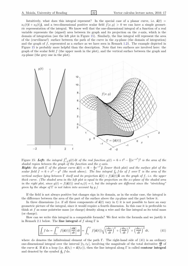
A. Moiola, University of Reading 32 Vector calculus lecture notes, 2016–17
Intuitively, what does this integral represent? In the special case of a planar curve, i.e. ~a(t) =a1(t)ı + a2(t), and a two-dimensional positive scalar field f(x, y) > 0 we can have a simple geomet-ric representation of the integral. We know well that the one-dimensional integral of a function of a realvariable represents the (signed) area between its graph and its projection on the x-axis, which is thedomain of integration (see the left plot in Figure 15). Similarly, the line integral will represent the areaof the (curvilinear!) surface between the path of the curve in the xy-plane (the domain of integration)and the graph of f , represented as a surface as we have seen in Remark 1.21. The example depicted inFigure 15 is probably more helpful than the description. Note that two surfaces are involved here: thegraph of the scalar field f (the upper mesh in the plot), and the vertical surface between the graph andxy-plane (the grey one in the plot).
t
g(t)
2−2 −2
−1
0
1
2
−2
−1
0
1
2
0
2
4
6
8
10
12
xy
f(x, y)
Γ = ~a(t)
Figure 15: Left: the integral∫ 2
−2g(t) dt of the real function g(t) = 6 + t2 − 9
4 (e−x2
)2 is the area of theshaded region between the graph of the function and the x-axis.Right: the path Γ of the planar curve ~a(t) = tı − 3
2e−t2 (lower thick plot) and the surface plot of the
scalar field f = 6 + x2 − y2 (the mesh above). The line integral∫Γf ds of f over Γ is the area of the
vertical surface lying between Γ itself and its projection ~a(t) + f(~a(t))k on the graph of f , i.e. the upperthick curve. (The shaded area in the left plot is equal to the projection on the xz-plane of the shaded areain the right plot, since g(t) = f(~a(t)) and a1(t) = t, but the integrals are different since the “stretching”given by the shape of Γ is not taken into account by g.)
If the field is not always positive but changes sign in its domain, as in the scalar case, the integral isthe difference between the area of the part of the surface above the xy-plane and the part below it.
In three dimensions (i.e. if all three components of ~a(t) vary in t) it is not possible to have an easygeometric picture of the integral, since it would require a fourth dimension. In this case it is preferable tothink at f as some pointwise mass (or charge) density along a wire and the line integral as its total mass(or charge).
How can we write this integral in a computable formula? We first write the formula and we justify itin Remark 2.1 below. The line integral of f along Γ is
∫
Γ
f ds =
∫ tF
tI
f(~a(t)
)∣∣∣∣d~a
dt
∣∣∣∣ dt =
∫ tF
tI
f(~a(t)
)√(da1
dt
)2+(da2dt
)2+(da3dt
)2dt, (41)
where ds denotes the infinitesimal element of the path Γ. The right-hand side of (41) is an ordinaryone-dimensional integral over the interval [tI , tF ], involving the magnitude of the total derivative d~a
dt ofthe curve ~a. If ~a is a loop (i.e. ~a(tI) = ~a(tF )), then the line integral along Γ is called contour integraland denoted by the symbol
∮Γ f ds.

A. Moiola, University of Reading 33 Vector calculus lecture notes, 2016–17
⋆ Remark 2.1 (Justification of the line integral formula (41)). To justify formula (41) we recall Riemann’ssums for one-dimensional integrals (in a very simple case), which you might have already seen in other courses.Consider a “well-behaved” function g : [0, 1] → R. Given a natural number N ∈ N, we can split thedomain [0, 1] in N subintervals [0, 1
N ], [ 1N ,2N ], . . . , [N−1
N , NN ] with equal lengths (see Figure 16). In each smallsubinterval we approximate g(t) with the constant function taking the value of g at the right extreme of thesubinterval, i.e. g(j/N). If the intervals are small enough, or equivalently if N is large enough, the integralof g on the subinterval is approximated by the integral of this constant function (which is simply g(j/N)/N ,since the length of the interval is j/N − (j − 1)/N = 1/N). Summing over the N subintervals, we obtain anapproximation of the integral of g over [0, 1], (see Figure 16):
∫ 1
0
g(t) dt =
N∑
j=1
∫ j/N
(j−1)/N
g(t) dt ≈N∑
j=1
g( jN
)∣∣∣j
N− j − 1
N
∣∣∣ =1
N
N∑
j=1
g( jN
), (42)
(here the symbol “≈” means “is approximately equal to”). If the integrand g is sufficiently “well-behaved” (forexample it is continuous in the closed interval [0, 1]), the approximation will actually converge to the desiredintegral, i.e.
∫ 1
0
g(t) dt = limN→∞
1
N
N∑
j=1
g( jN
).
This is the basic idea behind Riemann sums (although more general partitions of the interval and points ofevaluation may be taken).
x
g(x)
0 11N
2N
N−1N
Figure 16: The approximation of the integral of a real variable function g : [0, 1] → R by Riemann sums.The area of the grey part bounded by the plot of the integrand represents the integral of g, the area coveredwith diagonal lines is its Riemann sum approximation as in equation (42).
How can we write Riemann sums for the line integral of a scalar field? Consider a path Γ parametrised bythe curve ~a : [0, 1] → R3 and a scalar field f (both sufficiently smooth). Fix N ∈ N; for all integers 1 ≤ j ≤ Ncall Γj the sub-path parametrised by the curve ~a restricted to the subinterval [(j − 1)/N, j/N ]. We repeatthe same procedure used for scalar functions: we use the additivity of the integral to split it in a sum overthe sub-paths (step (i) in the equation below) and we approximate the integrals with those of the constantf(~a(j/n)), (ii). To compute the integrals of these constants we need to know the lengths of each sub-path Γj
(iii) (compare with the assumptions made in (40)). We approximate again the length of Γj with the distancebetween its endpoints ~a((j − 1)/N) and ~a(j/N), (iv). We multiply and divide by 1/N (v) and we note thatthe ratio obtained is a difference quotient approximating the total derivative of ~a(t) at t = j/N (vi). Usingthe Riemann sum (42) for real functions, we see that the formula obtained is an approximation of the integralin (41) and we conclude (vii)–(viii). In formulas:
∫
Γ
f ds(i)=
N∑
j=1
∫
Γj
f ds
(ii)≈N∑
j=1
∫
Γj
f(~a( jN
))ds
(iii)=
N∑
j=1
f(~a( jN
))Length(Γj)

A. Moiola, University of Reading 34 Vector calculus lecture notes, 2016–17
(iv)≈N∑
j=1
f(~a( jN
)) ∣∣∣~a( jN
)− ~a( j − 1
N
)∣∣∣
(v)=
1
N
N∑
j=1
f(~a( jN
))∣∣∣~a(
jN
)− ~a(
j−1N
)∣∣∣jN − j−1
N
(vi)≈ 1
N
N∑
j=1
f(~a( jN
)) ∣∣∣d~a
dt
( jN
)∣∣∣
(vii)≈N∑
j=1
∫ j/N
(j−1)/N
f(~a(t)
)∣∣∣d~a
dt(t)∣∣∣ dt
(viii)=
∫ 1
0
f(~a(t)
)∣∣∣d~a
dt(t)∣∣∣ dt.
We have derived (in a hand-waving way) formula (41) for the line integral of a scalar field, using only theRiemann sums for functions of real variable and the fundamental properties of the integrals stated in (40).
In this class we take the line integral formula (41) (and all the similar formulas for double, triple, surfaceand flux integrals in the rest of Section 2) as a definition; however, as we have seen, these can be (rigorously)derived from the general theory of Riemann integration.
Example 2.2 (Length of a path). Integrating the constant field f = 1 (cf. (40)), we see that the length of apath Γ is
length(Γ) =
∫
Γ
ds =
∫ tF
tI
∣∣∣∣d~a
dt
∣∣∣∣ dt. (43)
The line integral in (41) measures a quantity f distributed along Γ, thus it must be independent ofthe special parametrisation ~a. This is guaranteed by the factor
∣∣d~adt
∣∣, which takes into account the“speed” of travel along Γ (if we think at the parameter t as time). Similarly, the travel direction alongΓ (the curve orientation) does not affect the value of the line integral. In other words, f and Γ uniquelydefine the value of the integral in (41), independently of the choice of ~a we use to compute it. This makesthe notation
∫Γf ds in (41) well-posed, without the need of specifying ~a. Example 2.3 demonstrates the
invariance of the line integral with respect to the parametrisation.
Example 2.3 (Independence of parametrisation). Consider the scalar field f = y and the unit half circle Ccentred at the origin and located in the half plane ~r = xı+ y, y ≥ 0, which can be defined by either of thetwo parametrisations
~a : [0, π] → R3, ~a(t) = cos tı+ sin t, ~b : [−1, 1] → R3, ~b(τ) = τ ı +√1− τ2;
(see Figure 17). Verify that ∫ π
0
f(~a(t)
)∣∣∣∣d~a
dt
∣∣∣∣ dt =∫ 1
−1
f(~b(τ)
)∣∣∣∣d~b
dτ
∣∣∣∣ dτ.
We start by computing the total derivatives of the two parametrisations
d~a
dt= − sin tı+ cos t,
d~b
dτ= ı+
−τ√1− τ2
,
and their magnitudes
∣∣∣∣d~a
dt
∣∣∣∣ =√sin2 t+ cos2 t = 1,
∣∣∣∣∣d~b
dτ
∣∣∣∣∣ =√1 +
τ2
1− τ2=
1√1− τ2
.
The values of the field f along the two curves are f(~a(t)) = sin t and f(~b(τ)) =√1− τ2. We compute the
two integrals and verify they give the same value:∫ π
0
f(~a(t)
)∣∣∣∣d~a
dt
∣∣∣∣ dt =∫ π
0
sin t 1 dt = − cos t
∣∣∣∣π
0
= 1− (−1) = 2,
∫ 1
−1
f(~b(τ)
)∣∣∣∣∣d~b
dτ
∣∣∣∣∣ dτ =
∫ 1
−1
√1− τ2
1√1− τ2
dτ =
∫ 1
−1
dτ = 2.
Note that, not only the two parametrisations travel along C with different speeds (~a has constant speed∣∣d~adt
∣∣ = 1, while ~b “accelerates” at the endpoints), but they also travel in opposite directions: ~a from right to
left and ~b from left to right.
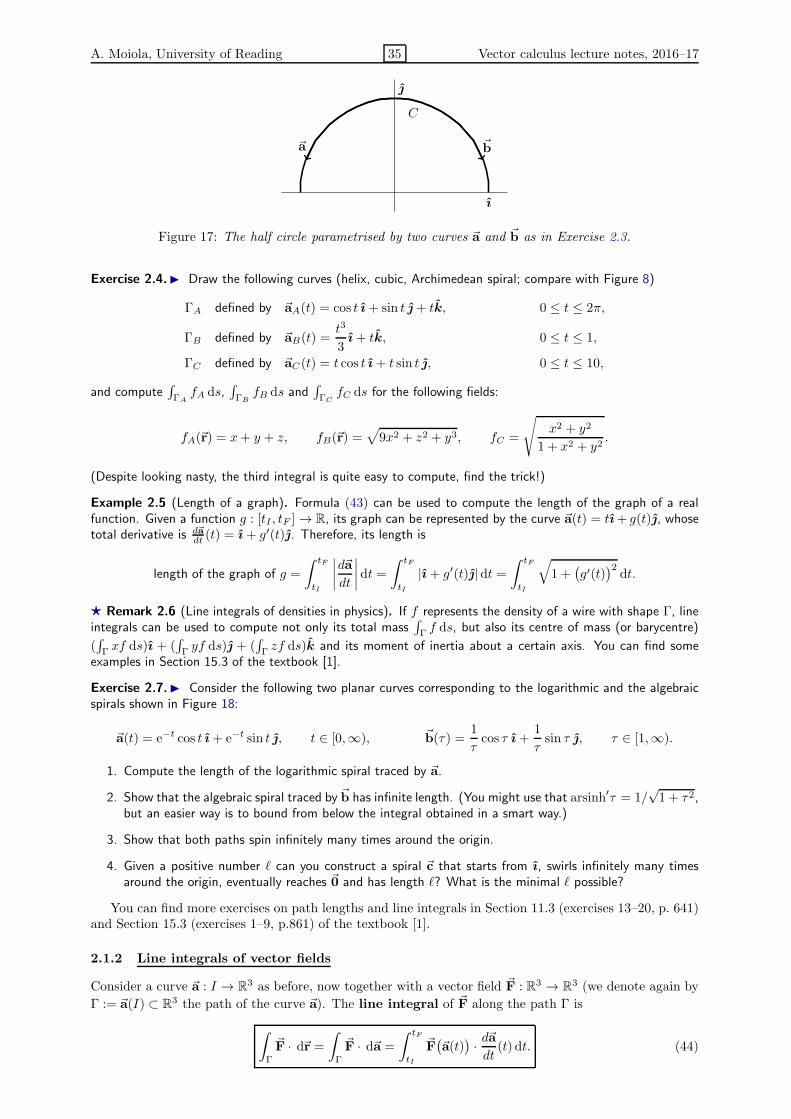
A. Moiola, University of Reading 35 Vector calculus lecture notes, 2016–17
ı
~b~a
C
Figure 17: The half circle parametrised by two curves ~a and ~b as in Exercise 2.3.
Exercise 2.4. Draw the following curves (helix, cubic, Archimedean spiral; compare with Figure 8)
ΓA defined by ~aA(t) = cos t ı+ sin t + tk, 0 ≤ t ≤ 2π,
ΓB defined by ~aB(t) =t3
3ı + tk, 0 ≤ t ≤ 1,
ΓC defined by ~aC(t) = t cos t ı+ t sin t , 0 ≤ t ≤ 10,
and compute∫ΓAfA ds,
∫ΓBfB ds and
∫ΓCfC ds for the following fields:
fA(~r) = x+ y + z, fB(~r) =√9x2 + z2 + y3, fC =
√x2 + y2
1 + x2 + y2.
(Despite looking nasty, the third integral is quite easy to compute, find the trick!)
Example 2.5 (Length of a graph). Formula (43) can be used to compute the length of the graph of a realfunction. Given a function g : [tI , tF ] → R, its graph can be represented by the curve ~a(t) = tı+ g(t), whosetotal derivative is d~a
dt (t) = ı+ g′(t). Therefore, its length is
length of the graph of g =
∫ tF
tI
∣∣∣∣d~a
dt
∣∣∣∣dt =∫ tF
tI
|ı+ g′(t)| dt =∫ tF
tI
√1 +
(g′(t)
)2dt.
⋆ Remark 2.6 (Line integrals of densities in physics). If f represents the density of a wire with shape Γ, lineintegrals can be used to compute not only its total mass
∫Γf ds, but also its centre of mass (or barycentre)
(∫Γxf ds)ı + (
∫Γyf ds) + (
∫Γzf ds)k and its moment of inertia about a certain axis. You can find some
examples in Section 15.3 of the textbook [1].
Exercise 2.7. Consider the following two planar curves corresponding to the logarithmic and the algebraicspirals shown in Figure 18:
~a(t) = e−t cos t ı+ e−t sin t , t ∈ [0,∞), ~b(τ) =1
τcos τ ı+
1
τsin τ , τ ∈ [1,∞).
1. Compute the length of the logarithmic spiral traced by ~a.
2. Show that the algebraic spiral traced by ~b has infinite length. (You might use that arsinh′τ = 1/√1 + τ2,
but an easier way is to bound from below the integral obtained in a smart way.)
3. Show that both paths spin infinitely many times around the origin.
4. Given a positive number ℓ can you construct a spiral ~c that starts from ı, swirls infinitely many timesaround the origin, eventually reaches ~0 and has length ℓ? What is the minimal ℓ possible?
You can find more exercises on path lengths and line integrals in Section 11.3 (exercises 13–20, p. 641)and Section 15.3 (exercises 1–9, p.861) of the textbook [1].
2.1.2 Line integrals of vector fields
Consider a curve ~a : I → R3 as before, now together with a vector field ~F : R3 → R3 (we denote again by
Γ := ~a(I) ⊂ R3 the path of the curve ~a). The line integral of ~F along the path Γ is
∫
Γ
~F · d~r =∫
Γ
~F · d~a =
∫ tF
tI
~F(~a(t)
)· d~adt
(t) dt. (44)

A. Moiola, University of Reading 36 Vector calculus lecture notes, 2016–17
-1 -0.8 -0.6 -0.4 -0.2 0 0.2 0.4 0.6 0.8 1
-0.4
-0.2
0
0.2
0.4
0.6
0.8
1
ı
~a(t)
~b(τ)
Figure 18: The logarithmic and the algebraic spirals of Exercise 2.7. We see that both swirls infinitelymany times around the origin but ~a approaches the origin itself much more quickly than ~b. Indeed thepath of ~a has finite length, while the length of the path of ~b is infinite.
The right-hand side of (44) is an ordinary one-dimensional integral (note that ~a, d~adt and ~F are vector-
valued but the integral is scalar since it contains a scalar product). If ~a is a loop, then the line integral of~F along Γ is called contour integral or circulation and denoted by the symbol
∮Γ~F · d~r.
Similarly to scalar fields, different parametrisations of Γ give the same integral, if the travel directionis the same. If the curve orientation is reversed, the sign of the integral changes (recall that thesign does not change for line integrals of scalar fields!):
if ~b(t) = ~a(1− t) then ~a([0, 1]) = ~b([0, 1]) = Γ and
∫
Γ
~F(~b) · d~b = −∫
Γ
~F(~a) · d~a.
The sign change follows from d~bdt (t) = − d~a
dt (1 − t) (when ~b(t) = ~a(1 − t)). Example 2.10 demonstratesthe invariance of the line integral and the sign change. Since, up to orientation, all the parametrisationsof Γ give the same integral for a given field, we can denote the line integral itself by
∫Γ~F · d~r, forgetting
the dependence on the parametrisation ~a. In this notation, Γ is an oriented path, namely a path witha given direction of travelling; if we want to consider the integral taken in the reverse direction we cansimply write
∫−Γ
~F · d~r = −∫Γ~F · d~r. (In this notation, Γ and −Γ are two different oriented paths sharing
the same support.)
The integral in (44) represents the integral along Γ of the component of ~F tangential to Γitself. To see this, for a smooth curve ~a : [tI , tF ] → R3 (under the assumption d~a
dt (t) 6= ~0 for all t), wedefine the unit tangent vector τ :
τ = τ1 ı+ τ2+ τ3k =1∣∣d~adt
∣∣d~a
dt=
da1
dt ı+da2
dt +da3
dt k√(da1
dt
)2+(da2
dt
)2+(da3
dt
)2 .
This is a vector field of unit length defined on Γ and tangent to it at every point. As mentioned, the lineintegral of the vector field ~F is equal to the line integral of the scalar field (~F · τ ), the projection of ~F onthe tangent vector of Γ:
∫
Γ
~F · d~r (44)=
∫ tF
tI
~F · d~adt
dt =
∫ tF
tI
(~F ·
d~adt∣∣d~adt
∣∣
)∣∣∣∣d~a
dt
∣∣∣∣ dt =∫ tF
tI
(~F · τ )∣∣∣∣d~a
dt
∣∣∣∣ dt(41)=
∫
Γ
(~F · τ ) ds. (45)
This an important relation between the main definitions of Sections 2.1.1 and 2.1.2.
Remark 2.8. We introduce a notation that will be used in Section 3 and is often found in books. The lineintegrals of a scalar field f with respect to the elements dx, dy and dz (over the oriented path Γ = ~a([tI , tF ]))are defined as
∫
Γ
f dx :=
∫
Γ
f ı · d~r (45)=
∫
Γ
f (ı · τ ) ds (44)=
∫ tF
tI
f(~a(t)
)da1dt
(t) dt,

A. Moiola, University of Reading 37 Vector calculus lecture notes, 2016–17
∫
Γ
f dy :=
∫
Γ
f · d~r (45)=
∫
Γ
f ( · τ ) ds (44)=
∫ tF
tI
f(~a(t)
)da2dt
(t) dt, (46)
∫
Γ
f dz :=
∫
Γ
f k · d~r (45)=
∫
Γ
f (k · τ ) ds (44)=
∫ tF
tI
f(~a(t)
)da3dt
(t) dt.
Therefore, we can expand the line integral of a vector field ~F = F1 ı + F2 + F3k as the sum of the integralsof its components:
∫
Γ
~F · d~r =
∫
Γ
F1 dx+
∫
Γ
F2 dy +
∫
Γ
F3 dz =
∫
Γ
(F1 dx+ F2 dy + F3 dz
). (47)
One can also use the formal identity dx = dxdt dt, identify x = a1(t) and obtain dx = da1(t)
dt dt, which givesagain the first equation in (46) (and similarly for the remaining two).
If the path Γ can be parametrised by the coordinate x, then it is possible to write the integral∫Γ f dx more
explicitly. Assume Γ to be parametrised by ~a(x) = xı+ y(x), for xL < x < xR and for a continuous functiony : (xL, xR) → R (here it is important that the parametrisation satisfies da1
dx = 1). Then, the line integral∫Γf dx can be written as the one-dimensional integral in x of the field evaluated along the graph of y(x):
∫
Γ
f dx(46)=
∫ xR
xL
f(~a(x)
)ı · d~adx
(x) dx =
∫ xR
xL
f(x, y(x)
)da1dx
(x) dx =
∫ xR
xL
f(x, y(x)
)dx. (48)
In other words, the integral∫Γ f dx is a standard integral in x if the path Γ is parametrised by a curve whose
first component is a1(x) = x + λ for some λ ∈ R. This fact also extends to curves in three dimensions. Ifthe path is run in the opposite direction (right to left, or from higher to lower values of x) with a similarparametrisation, then the sign of the integral is reversed, as expected.
⋆ Remark 2.9 (Work). In physics, the line integral of a force field ~F along a curve ~a, representing the
trajectory of a body, is the work done by ~F.
Example 2.10 (Integrals of a vector field along curves with common endpoints). Consider the following fivecurves, all connecting the points ~u = ~0 and ~w = ı + :
~aA(t) = tı+ t, 0 ≤ t ≤ 1,
~aB(t) = sin t ı+ sin t , 0 ≤ t ≤ π
2,
~aC(t) = e−tı+ e−t, 0 ≤ t <∞,
~aD(t) = t2ı+ t4, 0 ≤ t ≤ 1,
~aE(t) =
tı, 0 ≤ t ≤ 1,
ı+ (t− 1), 1 < t ≤ 2.
The curves ~aA and ~aB run along the diagonal of the square S = ~r s.t. 0 ≤ x ≤ 1, 0 ≤ y ≤ 1 at differentspeeds; ~aC travels along the same diagonal but in the opposite direction and in infinite time; ~aD and ~aE tracedifferent paths (see Figure 19). Note that ~aE is not smooth. Compute
∫Γn
~F · d~an for ~F = 2yı − x and
n = A,B,C,D,E, where Γn is the trajectory described by ~an (thus ΓA = ΓB = ΓC 6= ΓD 6= ΓE).We begin by computing the total derivatives of the curves
d~aAdt
= ı+ ,d~aBdt
= cos t ı+ cos t ,d~aCdt
= −e−tı− e−t,d~aDdt
= 2tı+ 4t3,
d~aEdt
=
ı 0 ≤ t ≤ 1,
1 < t ≤ 2.
Now we insert them in formula (44):
∫
ΓA
~F · d~aA =
∫ 1
0
(2y(t)ı− x(t)
)· (ı+ ) dt =
∫ 1
0
(2tı− t
)· (ı+ ) dt =
∫ 1
0
t dt =t2
2
∣∣∣∣1
0
=1
2,
∫
ΓB
~F · d~aB =
∫ π2
0
(2 sin t ı− sin t
)· (cos t ı+ cos t ) dt
=
∫ π2
0
sin t cos t dt =
∫ π2
0
1
2sin 2t dt =
− cos 2t
4
∣∣∣∣
π2
0
=1
4+
1
4=
1
2,
∫
ΓC
~F · d~aC =
∫ ∞
0
(2e−tı− e−t
)· (−e−tı− e−t) dt =
∫ ∞
0
(−e−2t) dt =e−2t
2
∣∣∣∣∞
0
=0− 1
2= −1
2,

A. Moiola, University of Reading 38 Vector calculus lecture notes, 2016–17
∫
ΓD
~F · d~aD =
∫ 1
0
(2t4ı− t2) · (2tı+ 4t3) dt =
∫ 1
0
(4t5 − 4t5) dt = 0,
∫
ΓE
~F · d~aE =
∫ 1
0
(−t) · ı dt+∫ 2
1
(2(t− 1)ı−
)· dt = 0 +
∫ 2
1
(−1) dt = −1,
As expected, we have∫
ΓA
~F · d~aA =
∫
ΓB
~F · d~aB = −∫
ΓC
~F · d~aC =1
26=∫
ΓD
~F · d~aD = 0 6=∫
ΓE
~F · d~aE = −1,
since the first and the second are different parametrisations of the same path, the third is a parametrisation ofthe same path with reverse direction, while the last two correspond to different paths.
−0.2 0 0.2 0.4 0.6 0.8 1 1.2
0
0.2
0.4
0.6
0.8
1
~u
~w~F
ΓA
ΓD
ΓE
Figure 19: The vector field ~F = 2yı − x and the curves described in Example 2.10. Note that ~F isperpendicular to ΓD in each point (thus
∫ΓD
~F · d~aD =∫ΓD
0 ds = 0) and to ΓE in its horizontal segment.
Exercise 2.11. Compute the line integral of ~G = xı+ y2 along the five curves described in Example 2.10.(Hint: recall the derivative of sin3 t.)
Exercise 2.12. Compute the line integrals of the position vector ~F(~r) = ~r along the two spirals defined inExercise 2.7. Can you guess the signs of the integrals before computing them?
To practise more on line integrals of vector fields, see e.g. Problems 1–9 of [1, Section 15.4, p. 869].
⋆ Remark 2.13 (Line integrals of vector fields as limits of Riemann sums). An intuitive explanation of the
relation between formula (44) and its interpretation as integral of the tangential component of ~F, can beobtained by considering a discrete approximation of the line integral with Riemann sums (similarly to what wehave already done in Remark 2.1 for integrals of scalar fields). Consider the times 0 = t0 < t1 < · · · < tN−1 <tN = 1, for i = 0, . . . , N , and the corresponding points ~ai = ~a(ti) ∈ Γ. Define the increments δ~ai := ~ai−~ai−1
and δti := ti − ti−1. Then, the integral of the component of ~F tangential to Γ in the interval (ti−1, ti) is
approximated by ~F(~ai) · δ~ai (recall the projection seen in Section 1.1.1), as depicted in Figure 20, and theintegral on Γ is approximated by the sum of these terms:
∫
Γ
~F(~a) · d~r ≈N∑
i=1
~F(~ai) · δ~ai =N∑
i=1
~F(~ai) ·δ~aiδti
δti.
In the limit N → ∞ (if the times ti are “well spaced” and ~a is smooth), δ~ai
δtitends to the total derivative of ~a
and the sum of δti gives the integral in dt, similarly to (42). Thus we recover formula (44).
2.1.3 Independence of path and line integrals for conservative fields
We consider the line integral of the gradient of a smooth scalar field ϕ along a curve ~a : [tI , tF ] → Γ ⊂ R3.Using the chain rule, since the function t 7→ ϕ(~a(t)) is a real function of real variable and the usualfundamental theorem of calculus applies, we obtain
∫
Γ
(~∇ϕ) · d~r (44)=
∫ tF
tI
~∇ϕ(~a(t)
)· d~adt
(t) dt(37)=
∫ tF
tI
d(ϕ(~a)
)
dt(t) dt = ϕ
(~a(tF )
)− ϕ
(~a(tI)
).

A. Moiola, University of Reading 39 Vector calculus lecture notes, 2016–17
x
y
z~a0
~a1
~ai−1~ai
~aNΓ
δ~ai
~F(~ai)
~F(~a1)
Figure 20: A schematic representation of the approximation of the line integral of the vector field ~F alongΓ using discrete increments (see Remark 2.13).
This is a simple but important result and we state it as a theorem. It is often called “fundamental theoremof vector calculus” (or “gradient theorem”), in analogy to the similar theorem known from one-dimensionalcalculus. This is the first relation between differential operators and integration we encounter; we will seeseveral others in Section 3 (see also the comparisons in Table 3 and in Appendix A).
Theorem 2.14 (Fundamental theorem of vector calculus). Consider a conservative vector field ~F with scalarpotential ϕ and a (piecewise smooth) curve ~a : [tI , tF ] → Γ ⊂ R3. Then
∫
Γ
~F · d~r =∫
Γ
(~∇ϕ) · d~r = ϕ(~a(tF )
)− ϕ
(~a(tI)
). (49)
The only information on the path Γ contained in the right-hand side of equation (49) are its endpoints
~a(tI) and ~a(tF ): the actual path Γ is not needed to compute the line integral of ~F on it (once we know thescalar potential ϕ). This means that line integrals of conservative fields are independent of theparticular integration path, but depend only on the initial and the final points of integration. Thus,given a conservative field ~F and two points ~p and ~q in its domain, we can use the notation
∫ ~q
~p
~F · d~r :=
∫
Γ
~F · d~r,
where Γ is any path connecting ~p to ~q. (Note that∫ ~q
~p is not well-defined for non-conservative fields.)
Comparison with scalar calculus 2.15. The fundamental theorem of calculus states that∫ b
a g(t) dt = G(b)−G(a) for all continuous real functions g : [a, b] → R, where G is a primitive of g, namely G′ = g. Similarly, the
fundamental theorem of vector calculus gives∫ ~q
~p~F · d~r = ϕ(~a(tF )) − ϕ(~a(tI)), where ϕ is a scalar potential
of the vector field ~F. So we can consider scalar potentials as the line-integral equivalent of primitives. Recallalso that both primitives and scalar potentials are defined up to constants.
Example 2.16. From Example 2.10 and formula (49), we immediately deduce that ~F = 2yı − x is notconservative, since integrals on different paths connecting the same endpoints give different values. The field~G = xı + y2 of Exercise 2.11 might be conservative as its integral has the same value along three differentcurves; however, in order to prove it is conservative we should proceed as we did in Example 1.67.
Exercise 2.17. Use formula (49), together with the results of Example 1.67 and Exercise 1.68, to compute
∫
Γ
~r · d~r and
∫
Γ
(zı+ xk) · d~r,
where Γ is any path connecting the point ~p = + 2k to the point ~q = −ı− − k.
In the next theorem we use path integrals to prove what was mentioned in Remark 1.70: whilethe implication “conservative ⇒ irrotational” is true for all vector fields, its converse “irrotational ⇒conservative” holds for fields defined on suitable domains. We define a star-shaped domain (or star-like) to be a domain D such that for all ~r ∈ D the straight segment connecting the origin to ~r lies entirelyinside D. All convex shapes, such as parallelepipeds and balls, containing the origin are star-shaped.

A. Moiola, University of Reading 40 Vector calculus lecture notes, 2016–17
Theorem 2.18. Let D be a star-shaped domain, and ~F be an irrotational vector field defined on D. Then, ~Fis conservative and a scalar potential is given by Φ(~r) =
∫Γ~r
~F · d~r, where Γ~r is the segment connecting the
origin to ~r.
Proof. Given ~r ∈ D, ~r 6= 0, a parametrisation of the segment Γ~r is ~a(t) = t~r for 0 ≤ t ≤ 1 (recall Remark
1.24). We note that ∂F2
∂x = ∂F1
∂y and ∂F3
∂x = ∂F1
∂z because ~F is irrotational. Using this, together with productand chain rule, we can compute the partial derivative of Φ in x:
∂Φ
∂x(~r) =
∂
∂x
∫
Γ~r
~F · d~r (from the definition of Φ)
=∂
∂x
∫ 1
0
~F(t~r) ·~rdt (from the parametrisation of Γ~r)
=
∫ 1
0
∂
∂x
(xF1(t~r) + yF2(t~r) + zF3(t~r)
)dt
=
∫ 1
0
(F1(t~r) + x
∂(F1(t~r)
)
∂x+ y
∂(F2(t~r)
)
∂x+ z
∂(F3(t~r)
)
∂x
)dt (from product rule)
=
∫ 1
0
(F1(t~r) + tx
∂F1
∂x(t~r) + ty
∂F2
∂x(t~r) + tz
∂F3
∂x(t~r)
)dt (from chain rule)
=
∫ 1
0
(F1(t~r) + tx
∂F1
∂x(t~r) + ty
∂F1
∂y(t~r) + tz
∂F1
∂z(t~r)
)dt (from ~∇× ~F = ~0)
=
∫ 1
0
(F1(t~r) + t~r · ~∇F1(t~r)
)dt
=
∫ 1
0
(F1(t~r) + t
d
dtF1(t~r)
)dt (chain rule (37) and
d~a
dt= ~r)
=
∫ 1
0
d
dt
(t F1(t~r)
)dt (from the product rule for
d
dt)
= 1F1(~r)− 0F1(~0) = F1(~r).
Similar identities can easily be derived for the derivatives in y and z, so we obtain ~∇Φ = ~F, i.e. Φ is ascalar potential of ~F and this is conservative.
In next Theorem 2.19, we use the fundamental theorem of vector calculus 2.14 to characterise conser-vative fields as those fields whose line integrals only depend on the endpoints. The proof of this theoremalso provides a construction of the scalar potential.
Theorem 2.19. Consider a continuous vector field ~F. The following three conditions are equivalent:
(i) ~F is conservative;
(ii) for all loops Γ ∮
Γ
~F · d~r = 0;
(iii) for all pairs of paths ΓA and ΓB with identical endpoints∫
ΓA
~F · d~r =∫
ΓB
~F · d~r.
⋆ Proof. [(i)⇒(ii)] If ~F is conservative, then ~F = ~∇ϕ for some scalar potential ϕ. If the loop Γ isparametrised by ~a : [tI , tF ] → Γ ⊂ R3 with ~a(tI) = ~a(tF ), then by the fundamental theorem of vector
calculus (49) we have∮Γ~F · d~r = ϕ(~a(tF ))− ϕ(~a(tI)) = 0.
[(ii)⇒(iii)] Assume condition (ii) is satisfied. The two paths ΓA and ΓB can be combined in a loop13
Γ = ΓA − ΓB (see Figure 21). Using the additivity property (40), the difference between the two pathintegrals is then
∫
ΓA
~F · d~r−∫
ΓB
~F · d~r =
∫
ΓA
~F · d~r+∫
−ΓB
~F · d~r =∮
Γ
~F · d~r = 0,
13As we have done in Section 2.1.2, here we consider all paths Γ to be “oriented” paths, i.e. paths equipped with a preferreddirection of travel (orientation). We denote by −Γ the same path as Γ with the opposite orientation. If Γα and Γβ are pathssuch that the final point of Γα coincides with the initial point of Γβ , we denote by Γα + Γβ their “concatenation”, i.e., thepath corresponding to their union (obtained travelling first along Γα and then along Γβ). Thus ΓA−ΓB is the concatenationobtained travelling first along ΓA and then along ΓB , the latter run in the opposite direction,

A. Moiola, University of Reading 41 Vector calculus lecture notes, 2016–17
which is condition (iii).
[(iii)⇒(i)] Fix a point ~r0 in the domain of ~F. Then, for all points ~r, the scalar field Φ(~r) :=∫ ~r~r0~F · d~r
is well-defined (does not depend on the integration path). Consider the partial derivative
∂Φ
∂x(~r) = lim
h→0
1
h
(Φ(~r+ hı)− Φ(~r)
)= lim
h→0
1
h
(∫ ~r+hı
~r0
~F · d~r−∫ ~r
~r0
~F · d~r).
Since in the integrals we can choose any path, in the first integral we consider the path passing through ~rand moving in the x direction along the segment with endpoints ~r and ~r+hı. This segment is parametrisedby ~a(t) = ~r+ tı for 0 ≤ t ≤ h (which has total derivative d~a
dt (t) = ı), thus
∂Φ
∂x(~r) = lim
h→0
1
h
(∫ ~r
~r0
~F · d~r+∫ ~r+hı
~r
~F · d~r−∫ ~r
~r0
~F · d~r)
= limh→0
1
h
∫ ~r+hı
~r
~F · d~r
(44)= lim
h→0
1
h
∫ h
0
~F(~r+ tı) · ı dt
= limh→0
1
h
∫ h
0
F1
((x+ t)ı+ y+ zk
)dt
= limh→0
F1
((x+ τ )ı + y+ zk
)for some τ ∈ [0, h]
= F1(~r)
(using, in the last two equalities, the integral version of the mean value theorem for real continuous
functions 1b−a
∫ b
af(t) dt = f(τ) for a τ ∈ [a, b] and the continuity of F1). Similarly, ∂Φ
∂y = F2 and ∂Φ∂z = F3,
thus ~F = ~∇Φ. The vector field ~F is conservative and Φ is a scalar potential.
x
y
z
~p
~qΓA
ΓB
Figure 21: Two paths ΓA and ΓB connecting the points ~p and ~q and defining a loop Γ = ΓA − ΓB, as inTheorem 2.19.
We summarise what we learned here and in Section 1.5 about conservative fields in the following scheme:
~F = ~∇ϕ(conservative)
⇐⇒∫ ~q
~p
~F · d~ris path independent
⇐⇒
∮
Γ
~F · d~r = 0
∀ loops Γ=⇒
~∇× ~F = ~0(irrotational)
(50)
If the domain of definition of ~F is star-shaped, by Theorem 2.18 the converse of the last implication holds.
Exercise 2.20. Consider the two oriented paths from the point ı to the point (see Figure 22):
Γa :=xı + y, x+ y = 1, x, y ≥ 0
, Γb :=
xı+ y, x2 + y2 = 1, x, y ≥ 0
,
and the vector field ~F(~r) = (x2 + y2)(ı + 2). Compute the line integrals∫Γa
~F · d~r,∫Γb
~F · d~r, and use the
values of these integrals to prove that ~F is not conservative.
⋆ Remark 2.21 (An irrotational, non-conservative field). In Remark 1.71, we have seen that the field
~F =−y
x2 + y2ı+
x
x2 + y2
is conservative in the half-space D = ~r ∈ R3 s.t. x > 0 and we have claimed (without justification) that noscalar potential can be defined in its larger domain of definition E = ~r ∈ R3 s.t. x2 + y2 > 0. We can easily

A. Moiola, University of Reading 42 Vector calculus lecture notes, 2016–17
x
y
ı
Γa
Γb
Figure 22: The paths Γa and Γb in Exercise (2.20).
compute the circulation of ~F along the unit circle C = ~r ∈ R3, s.t. x2 + y2 = 1, z = 0 (parametrised by~a(t) = cos t ı+ sin t with 0 ≤ t ≤ 2π):
∫
C
~F · d~r =∫ 2π
0
(− sin tı+ cos t) · (− sin tı+ cos t) dt =
∫ 2π
0
1 dt = 2π.
Since this integral is not equal to zero, Theorem 2.19 proves that ~F is not conservative in the domain E. (Wehave completed the proof of the claim made in Remark 1.71.)
⋆ Remark 2.22. From the results studied in this section we can learn the following idea. We already knowthat any continuous real functions f : (tI , tF ) → R can be written as the derivative of another function
F : (tI , tF ) → R (the primitive of f , F (t) =∫ t
t∗f(s) ds for some t∗), even if sometimes computing F may be
very difficult. Thus, the integral of f = F ′ can be evaluated as the difference of two values of F . Similarly,a scalar field g : D → R, D ⊂ R3, can be written as a partial derivative (with respect to a chosen direction)of another scalar field. On the other hand, only some vector fields can be written as gradients of a scalar field(the potential) and their line integral computed as differences of two evaluations of the potential. These areprecisely the conservative fields, characterised by the conditions in box (50).
2.2 Multiple integrals
We have learned how to compute integrals of scalar and vector fields along curves. We now focus onintegrals on (flat and curved) surfaces and volumes.
2.2.1 Double integrals
For a two-dimensional region R ⊂ R2 and a scalar field f : R → R, we want to define and compute
∫∫
R
f(x, y) dA, (51)
namely the integral of f over R. The differential dA = dxdy represents the infinitesimal area element,which is the product of the infinitesimal length elements in the x and the y directions. Since the domainis two-dimensional, this is commonly called double integral.
The double integral∫∫
R f dA over a region R represents the (signed) volume of the portion ofspace delimited by the graph surface of the two-dimensional field f and the xy-plane; seeFigures 23 and 24. “Signed” means that the contribution given by the part of R in which f is negative issubtracted from the contribution from the part where f is positive.
In the same way as integrals of real functions are approximated by sums of areas of rectangles (recallFigure 16), double integrals are approximated by sums of volumes of parallelepipeds, see Figure 24.
For simplicity, we first consider only two-dimensional domains which can be written as
R =xı+ y ∈ R2, s.t. xL < x < xR, a(x) < y < b(x)
, (52)
for two functions a(x) < b(x) defined in the interval (xL, xR). The domains that can be expressed in thisway are called y-simple. These are the domains such that their intersection with any vertical line is eithera segment or the empty set. A prototypical example is shown in Figure 25. Examples of non-y-simpledomains are the C-shaped domain ~r s.t. 2y2 − 1 < x < y2, the “doughnut” ~r s.t. 1 < |~r| < 2 (drawthem!) and any other domain containing a hole. These and other more complicated non-y-simple domainscan be decomposed in the disjoint union of two or more y-simple or x-simple (similarly defined) domains.

A. Moiola, University of Reading 43 Vector calculus lecture notes, 2016–17
y
f(x, y)
x
R
Figure 23: The double integral∫∫
R f dA over a domain R (a triangle in the picture) represents the (signed)volume delimited by the graph of the two-dimensional field f (the upper surface) and the xy-plane.
1
0.8
0.60
00.4
0.2
0.4
0.5
0.20.6
0.80
1
1
1.5
1
0.8
0.60
00.4
0.2
0.4
0.5
0.20.6
0.80
1
1
1.5
Figure 24: The surface plot of the scalar field f =√x+ y/2 over the square Q = (0, 1) × (0, 1). The
double integral∫∫
Q f dA measures the volume shown in the left figure. If Q is partitioned in smaller squaresS1, . . . , Sn, the double integral can be approximated by the sum over j = 1, . . . , n of the volumes of theparallelepipeds with basis the small squares Sj and height the value of f at one point ~x ∈ Sj:
∫∫Qf dA ≈∑n
j=1 f(~xj)Area(Sj). In this example the integral is approximated by n = 25 parallelepipeds. In the limitn→ ∞ (i.e. more smaller squares), the sum converges to the desired integral. This is how double integralsare actually rigorously defined. Recall the similar argument made in Remark 2.1 for the case of lineintegrals. (In this example,
∫∫Q f dA =
√2(35/2−1−25/2)/15 ≈ 0.842, and
∑25j=1 f(~xj)Area(Sj) ≈ 0.734.)
xL xR
y = a(x)
y = b(x)
x
y
R
dydx
dA = dxdy
Figure 25: A y-simple two-dimensional domain R, bounded by the functions a and b in the interval(xL, xR), and the infinitesimal area element dA.

A. Moiola, University of Reading 44 Vector calculus lecture notes, 2016–17
In order to compute the integral (51), we view it as an iterated or nested integral.14 In other words,for each value of x ∈ (xL, xR), we first consider the one-dimensional integral of f along the segment parallelto the y-axis contained in R, i.e.
If (x) =
∫ b(x)
a(x)
f(x, y) dy.
Note that both the integrand and the integration endpoints depend on x. The integral If is a function ofx, but is independent of y; we integrate it along the direction x:
∫∫
R
f(x, y) dA =
∫ xR
xL
If (x) dx =
∫ xR
xL
(∫ b(x)
a(x)
f(x, y) dy
)dx. (53)
Of course, the role of x and y are exchanged in x-simple domains.We consider as concrete example the isosceles triangle
Q :=~r ∈ R2, s.t. 0 < y < 1− |x|
; (54)
see Figure 26. In this case, xL = −1, xR = 1, a(x) = 0, b(x) = 1− |x|. If we first integrate a field f alongthe y-axis and then along the x-axis, we obtain:∫∫
Q
f(x, y) dA =
∫ 1
−1
(∫ 1−|x|
0
f(x, y) dy
)dx =
∫ 0
−1
(∫ 1+x
0
f(x, y) dy
)dx+
∫ 1
0
(∫ 1−x
0
f(x, y) dy
)dx.
We can also consider the same triangle as an x-simple domain and first integrate along the x-axis andthen along the y-axis (right plot in Figure 26):
∫∫
Q
f(x, y) dA =
∫ 1
0
(∫ 1−y
y−1
f(x, y) dx
)dy.
Of course, the two integrals will give the same value.
xR = 1xL = −1
y = 1− xy = 1 + x
y = 0
Q
yR = 1
yL = 0
x = 1− yx = y − 1Q
Figure 26: The computation of the double integral∫∫
Qf(x, y) dA on the triangle Q. The left plot represents
∫ 1
−1(∫ 1−|x|0
f dy) dx, where the inner integral is taken along the shaded band (of infinitesimal width) andthe outer integral corresponds to the movement of the band along the x axis. The right plot represent the
integration where the variables are taken in the opposite order∫ 1
0(∫ 1−y
y−1f dx) dy.
To have a more concrete example, we compute the integral of f = x − y2 on the triangle Q in boththe ways described above:∫∫
Q
(x− y2) dA =
∫ 0
−1
(∫ 1+x
0
(x− y2) dy
)dx+
∫ 1
0
(∫ 1−x
0
(x − y2) dy
)dx
=
∫ 0
−1
(xy − 1
3y3)∣∣∣∣
1+x
y=0
dx+
∫ 1
0
(xy − 1
3y3)∣∣∣∣
1−x
y=0
dx
=
∫ 0
−1
−1
3
(x3 + 1
)dx+
∫ 1
0
(13x3 − 2x2 + 2x− 1
3
)dx
=(− 1
12x4 − 1
3x)∣∣∣∣
0
−1
+( 1
12x4 − 2
3x3 + x2 − 1
3x)∣∣∣∣
1
0
=1
12− 1
3+
1
12− 2
3+ 1− 1
3= −1
6;
∫∫
Q
(x− y2) dA =
∫ 1
0
(∫ 1−y
y−1
(x− y2) dx
)dy
=
∫ 1
0
(12x2 − xy2
)∣∣∣∣1−y
x=y−1
dy =
∫ 1
0
2(y3 − y2) dy =1
2y4 − 2
3y3∣∣∣∣1
0
= −1
6.
14You have already seen iterated integrals during the first year: see handout 5, from page 23 on, of the Calculus module.

A. Moiola, University of Reading 45 Vector calculus lecture notes, 2016–17
Exercise 2.23. Compute the following double integrals (drawing a sketch of the domain might be helpful):∫∫
R
e3y sinxdxdy where R = (0, π)× (1, 2) =xı+ y s.t. 0 < x < π, 1 < y < 2
,
∫∫
Q
y dxdy where Q is the triangle with vertices ~0, , 5ı+ ,
∫∫
S
cosxdxdy where S =xı+ y s.t. 0 < x <
π
2, 0 < y < sinx
.
You can find plenty of exercises on double integrals in Section 14.2 (p. 802, exercises 1–28) of [1].
2.2.2 Change of variables
Comparison with scalar calculus 2.24. We learned in first-year calculus how to compute one-dimensionalintegrals by substitution of the integration variable, for example
∫ 1
0
ex√1 + ex dx
ξ(x)=1+ex
dξ=ex dx=
∫ ξ(1)
ξ(0)
(ξ − 1)√ξdx
dξdξ =
∫ 1+e
2
√ξ dξ =
2
3ξ
32
∣∣∣∣1+e
2
=2
3(1 + e)
32 − 4
√2
3≈ 2.894.
How do we extend this technique to double integrals? In this one-dimensional example, the interval of inte-gration x ∈ (0, 1) is mapped15 into a new interval (2, 1 + e) (whose variable is denoted by ξ) by the changeof variable T : x 7→ ξ = 1 + ex, which is designed to make “simpler” (more precisely: easier to integrate) thefunction to be integrated. The factor dx/ dξ takes care of the “stretching” of the variable. In two dimensions,we can use a change of variables not only to make the integrand simpler, but also to obtain a domain ofintegration with a simpler shape (e.g. a rectangle instead of a curvilinear domain).
Consider a region R ⊂ R2 on which a two-dimensional, injective vector field ~T : R → R2 is defined.We can interpret16 this field as a “change of variables”, i.e. a deformation of the domain R into a newdomain ~T(R). We will informally call ~T a “transformation” or “mapping” of the region R. Departing
from the usual notation, we denote by ξ(x, y) and η(x, y) (“xi” and “eta”) the components of ~T. Weunderstand ξ and η as the Cartesian coordinates describing the transformed domain: R is a subset of theplane described by x and y, ~T(R) is a subset of the plane described by ξ and η. We denote by x(ξ, η) and
y(ξ, η) the components of the inverse transformation ~T−1 from the ξη-plane to the xy-plane17:
~T :R→ ~T(R) ~T−1 : ~T(R) → R
xı+ y 7→ ξ(x, y)ξ + η(x, y)η ξξ + ηη 7→ x(ξ, η)ı + y(ξ, η),
or, with a different notation,
(x, y) 7→(ξ(x, y), η(x, y)
)(ξ, η) 7→
(x(ξ, η), y(ξ, η)
).
For example, we consider the following (affine) change of variables18 ~T:
ξ(x, y) =−x− y + 1
2, η(x, y) =
x− y + 1
2,
whose inverse ~T−1 corresponds to x(ξ, η) = −ξ + η, y(ξ, η) = −ξ − η + 1.
(55)
(The transformation ~T associated to ξ and η is a combination of a translation of length 1 in the negativey direction, an anti-clockwise rotation of angle 3π/4, and a shrinking of factor
√2 in every direction.)
The triangle Q in (54) in the xy-plane is mapped by ~T into the triangle with vertices ~0, ξ and η in theξη-plane, as shown in Figure 27. Other examples of changes of coordinates are displayed in Figure 28.
15In case you are not familiar with the mathematical use of the verb “to map”, it is worth recalling it. Given a functionT defined in the set A and taking values in the set B (which we can simply write as T : A → B), we say that T “maps”an element a ∈ A into b ∈ B if T (a) = b, and “maps” the subset C ⊂ A into T (C) ⊂ B. Thus, a function is often called a“map” or a “mapping”; we will use this words to denote the functions related to changes of variables or operators. (If youthink about it, you see that a map in the non-mathematical meaning is nothing else than a function that associates to everypoint in a piece of paper a point on the surface of the Earth. We will also define “charts” to be some special maps from aflat surface to a curvilinear one.)
16Another simple and useful interpretation of a change of variables is the following. Each point ~r = xı + y ∈ R ⊂ R2 isidentified by two numbers, the coordinates x and y. A change of variables is simply a rule to associate to each point in Rother two numbers, the coordinates ξ and η.
17Here and in the following, we use the vectors ξ and η. They can be understood either as the unit vectors of the canonicalbasis of the ξη-plane (exactly in the same role of ı and in the xy-plane) or as vector fields with unit length, defined in R,pointing in the direction of increase of ξ and η, respectively. The first interpretation is more helpful at this stage, while thesecond will be useful in Section 2.3.
18This change of variables is “affine”, meaning that its components ξ and η are polynomials of degree one in x and y.Affine change of variables translate, rotate, dilate and stretch the coordinates but do not introduce curvature: straight linesare mapped into straight lines.

A. Moiola, University of Reading 46 Vector calculus lecture notes, 2016–17
x+y −
1=0x
− y+1=0
y = 0 x
y
Q
~T
ξ
η
~T(Q)
1−ξ −η=y=0
−2ξ=x+y−1=
0
2η = x− y + 1 = 0
Figure 27: The triangle Q in the xy-plane and in the ξη-plane. Along the edges are shown the equationsof the corresponding lines.
0 0.5 10
0.2
0.4
0.6
0.8
1
0 0.5 1
0
0.2
0.4
0.6
0.8
1
0.5 1 1.5 20
0.5
1
1.5
−1 0 1 2
−2
−1.5
−1
−0.5
0
0.5
1
ξξ
ξ
ηη
η
Figure 28: The unit square 0 < x, y < 1 (upper left) under three different mappings: ξ = x, η = y +15 sin(2πx) (upper right); ξ = (1+ x) cos y, η = (1+ x) sin y (lower left); ξ = exy cos(2πy), η = exy sin(2πy)(lower right).
A transformation ~T : (x, y) 7→ (ξ, η) warps and stretches the plane, if we want to compute an integralin the transformed variables we need to take this into account. The infinitesimal area element dA = dxdyis modified by the transformation in the ξη-plane.
We recall that the Jacobian matrices of ~T and ~T−1 are 2× 2 matrix fields containing their first orderpartial derivatives (see Section 1.3.3). We denote their determinants by
∂(ξ, η)
∂(x, y):= det(J ~T) =
∂ξ
∂x
∂η
∂y− ∂ξ
∂y
∂η
∂x, and
∂(x, y)
∂(ξ, η):= det
(J(~T−1)
)=∂x
∂ξ
∂y
∂η− ∂y
∂ξ
∂x
∂η. (56)
These are called Jacobian determinants19; their absolute values are exactly the factors needed tocompute double integrals under the change of coordinates ~T:
∫∫
R
f(x, y) dxdy =
∫∫
~T(R)
f(x(ξ, η), y(ξ, η)
)∣∣∣∣∂(x, y)
∂(ξ, η)
∣∣∣∣dξ dη, (57)
for any scalar field f : R → R. This is the fundamental formula for the change of variables in a doubleintegral. In other words, we can say that the infinitesimal surface elements in the xy-plane and in the
19In some books, when used as noun, the word “Jacobian” stands for Jacobian determinant, as opposed to Jacobianmatrix. Again, this can be a source of ambiguity.

A. Moiola, University of Reading 47 Vector calculus lecture notes, 2016–17
ξη-plane are related to each other by the formulas:
dxdy =
∣∣∣∣∂(x, y)
∂(ξ, η)
∣∣∣∣ dξ dη, dξ dη =
∣∣∣∣∂(ξ, η)
∂(x, y)
∣∣∣∣dxdy.
We also have∂(ξ, η)
∂(x, y)=
1∂(x,y)∂(ξ,η)
. (58)
Formula (58) is often useful when the partial derivatives of only one of the transformations ~T and ~T−1
are easy to compute. In other words, if you need ∂(x,y)∂(ξ,η) for computing an integral via a change of variable
as in (57), but J ~T is easier to obtain than J(~T)−1, you can compute ∂(ξ,η)∂(x,y) and then apply (58).
Comparison with scalar calculus 2.25. Recall that in the one-dimensional integration by substitution in 2.24
we use the factor dξdx . The corresponding factor for double integrals is the Jacobian determinant d(ξ,η)
d(x,y) (56).
⋆ Remark 2.26. Note that here we are implicitly assuming that the Jacobian matrices of ~T and ~T−1 arenever singular, i.e. their determinants do not vanish in any point of the domain, otherwise equation (58) would
make no sense. Under this assumption, it is possible to prove that J(~T−1) = (J ~T)−1, namely the Jacobian
matrix of the inverse transform is equal to the inverse matrix of the Jacobian of ~T itself; this is part of theInverse Function Theorem you might study in a future class.
We return to the affine transformations (55). Their Jacobian matrices are (recall the definition in (16))
J ~T =
(− 1
2 − 12
12 − 1
2
), J(~T−1) =
(−1 1−1 −1
).
Note that this case is quite special: since the transformations are affine (namely polynomials of degreeone), their Jacobian are constant in the whole plane R2. From this, we compute the Jacobian determinants
∂(ξ, η)
∂(x, y)=(− 1
2
)(− 1
2
)− 1
2
(− 1
2
)=
1
2,
∂(x, y)
∂(ξ, η)= (−1)(−1)− 1(−1) = 2. (59)
Note that, as expected, ∂(x,y)∂(ξ,η) = 2 is the ratio between the areas of Q and ~T(Q) (since in this simple case
the Jacobian of ~T and its determinant are constant in Q). Now we can easily integrate on the triangle Qin (54) the scalar field f = (1 − x − y)5, for example, using the change of variables (55) which maps Q
into ~T(Q) as in Figure 27:
∫∫
Q
f(x, y) dxdy(55),(57)
=
∫∫
~T(Q)
f(−ξ + η,−ξ − η + 1)
∣∣∣∣∂(x, y)
∂(ξ, η)
∣∣∣∣ dξ dη
(59)=
∫∫
~T(Q)
(1 + ξ − η + ξ + η − 1)5 2 dξ dη
=
∫∫
~T(Q)
(2ξ)5 2 dξ dη
(51)= 64
∫ 1
0
ξ5(∫ 1−ξ
0
1 dη
)dξ
= 64
∫ 1
0
(ξ5 − ξ6) dξ
= 64(16ξ6 − 1
7ξ7)∣∣∣∣
1
0
=64
42≈ 1.524.
Remark 2.27. Note that in all the formulas related to change of variables the domain of integration (appearingat subscript of the integral sign) must be a subset of the plane spanned by the integration variables (appearing inthe differential term d . . . d . . .). In the example above, the integral
∫∫Qis always associated to the differential
dxdy, meaning that Q is a set in the xy-plane; the integral∫∫
~T(Q)always appears with the differential dξ dη,
as ~T(Q) is a set in the ξη-plane.
Example 2.28 (Area of regions). As we required in (40), the area of a domain R ⊂ R2 can be computedby integrating on it the constant one: Area(R) =
∫∫R1 dxdy. If R is y-simple, one can use the iterated
integral (53). Otherwise, if R is complicated but can be mapped into a simpler shape, the change of variableformula (57) can be used to compute its area.

A. Moiola, University of Reading 48 Vector calculus lecture notes, 2016–17
We now want to use formula (57) to compute the areas of the curvilinear domains plotted in Figure 28. Eachof them is obtained from the unit square S = 0 < x < 1, 0 < y < 1 (upper left plot) from the transformationslisted in the figure caption. We denote the domains by RUR, RLL, RLR (as upper right, lower left and lowerright plot) to distinguish one another, and use a similar notation for the change of variable transformations
and coordinates (e.g. ~TUR : S → RUR). In the first case (upper right plot), the transformation, its Jacobianmatrix and determinant are
ξUR = x, ηUR = y +1
5sin(2πx), J ~TUR =
(1 0
25π cos(2πx) 1
),
∂(ξUR, ηUR)
∂(x, y)= 1.
From this we obtain
Area(RUR) =
∫∫
RUR
dξUR dηUR =
∫∫
~T−1
UR(RUR)
∂(ξUR, ηUR)
∂(x, y)dxdy =
∫ 1
0
∫ 1
0
1 dxdy = 1,
(which we could have guessed from the picture!). For the second picture we have
ξLL = (1 + x) cos y, ηLL = (1 + x) sin y,
J ~TLL =
(cos y −(1 + x) sin ysin y (1 + x) cos y
),
∂(ξLL, ηLL)
∂(x, y)= 1 + x,
which leads to
Area(RLL)=
∫∫
RLL
dξLL dηLL=
∫∫
S
∂(ξLL, ηLL)
∂(x, y)dxdy=
∫ 1
0
∫ 1
0
(1 + x) dy dx=
∫ 1
0
(1 + x) dx=3
2.
Exercise 2.29. Compute the area of the domain RLR in the lower-right plot of Figure 28, obtained fromthe unit square S = 0 < x < 1, 0 < y < 1 via the change of variables
ξLR = exy cos(2πy), ηLR = exy sin(2πy).
(If you do it in the right way, i.e. with no mistakes, despite looking nasty the computation is actually easy).
Exercise 2.30. (i) Draw the quadrilateral Q ⊂ R2 and compute its area:
Q =xı + y, such that x = (4− η)ξ, y = (π − ξ)η, for 0 < ξ < 1, 0 < η < 1
.
(ii) More generally, given two constants a, b ≥ 2 compute the area of
Qab =xı + y, such that x = (a− η)ξ, y = (b− ξ)η, for 0 < ξ < 1, 0 < η < 1
.
Exercise 2.31. Use the change of variables
ξ = ξ(x, y) = x
4 + y − 1,
η = η(x, y) = y − x4 ,
(60)
to compute the double integral∫∫
Pf(ξ, η) dξ dη, where f(ξ, η) = e−ξ−η, and where the two-dimensional
domain P in the ξη-plane is the square with vertices ξ, η,−ξ,−η.
⋆ Remark 2.32 (Intuitive justification of the change of variable formula). Where does the change of variableformula (57) come from? Why are the infinitesimal surface elements related to the Jacobian determinant?
Consider the square S with vertices
~pSW = xı + y, ~pSE= (x+ h)ı+ y, ~pNW = xı+ (y + h), ~pNE= (x+ h)ı+ (y + h),
where h > 0 is “very small”. Of course, it has area equal to |~pSE − ~pSW ||~pNW − ~pSW | = h2. Under atransformation (x, y) 7→ (ξ, η), the first three vertices are mapped into
~qSW = ξ(x, y)ξ + η(x, y)η,
~qSE = ξ(x+ h, y)ξ + η(x + h, y)η ≈(ξ(x, y) + h
∂ξ
∂x(x, y)
)ξ +
(η(x, y) + h
∂η
∂x(x, y)
)η,
~qNW = ξ(x, y + h)ξ + η(x, y + h)η ≈(ξ(x, y) + h
∂ξ
∂y(x, y)
)ξ +
(η(x, y) + h
∂η
∂y(x, y)
)η,
where we have approximated the values of the fields ξ and η with their Taylor’s expansions centred a xı + y(which is a good approximation if h is small).

A. Moiola, University of Reading 49 Vector calculus lecture notes, 2016–17
x
y
~pSW
= xı + y
~pNW ~pNE
~pSE
S h
h
ξ
η
~qSW
~qSE
~qNW~qNE
Figure 29: As described in Remark 2.32, the square S of area h2 in the xy-plane is mapped into acurvilinear shape in the ξη-plane. The Jacobian determinant (multiplied by h2) measures the area of thedashed parallelogram in the ξη-plane, which approximates the area of the image of S.
We then approximate the image of S in the ξη-plane with the parallelogram with edges [~qSE , ~qSW ] and[~qNW , ~qSW ], see Figure 29. Using the geometric characterisation of the vector product as in Section 1.1.2, wesee that this parallelogram has area equal to the magnitude of the vector product of two edges:
Area(~T(S)
)≈∣∣(~qSE − ~qSW )× (~qNW − ~qSW )
∣∣ =
∣∣∣∣(h∂ξ
∂xξ + h
∂η
∂xη)×(h∂ξ
∂yξ + h
∂η
∂yη)∣∣∣∣
= h2∣∣∣∣∂ξ
∂x
∂η
∂y− ∂η
∂x
∂ξ
∂y
∣∣∣∣ (61)
(56)= h2
∣∣∣∣∂(ξ, η)
∂(x, y)
∣∣∣∣.
Therefore, the Jacobian determinant is the ratio between the area of the parallelogram approximating the imageof S, and the area of the square S itself. In the limit h→ 0, the approximation error vanishes and the Jacobiandeterminant is thus equal to the ratio between the “infinitesimal areas” in the xy-plane and in the ξη-plane.When we perform the change of variables (x, y) 7→ (ξ, η) inside an integral, in order to preserve the value ofthe integral itself, we need to replace the contribution given by every “infinitesimally small” square S with the
contribution given by its transform, which is the same as multiplying with ∂(ξ,η)∂(x,y) .
To pass from an infinitesimal element to a finite domain, we use two-dimensional Riemann sums. Considera domain R partitioned in N disjoint small squares Sjj=1,...,N with area h2; for example R can be the
unit square in the upper left plot of Figure 28, where N = 25. The domain ~T(R) obtained by a change of
variables (x, y) 7→ (ξ, η) is composed of N curvilinear subdomains ~T(Sj)j=1,...,N , see e.g. one of the otherthree plots in Figure 28. Denoting by fj := f(~pj) the value of the integrand f (a continuous scalar field) ina point ~pj ∈ Sj , for all 1 ≤ j ≤ N , we can decompose the integral at the right-hand side of (57) over all thesubdomains and approximate each of them with the integral of the constant fj . Then, approximating the areaof each subdomain with (61), we obtain an approximation of the change of variables formula (57):
∫∫
~T(R)
f
∣∣∣∣∂(x, y)
∂(ξ, η)
∣∣∣∣ dξ dη =
N∑
j=1
∫∫
~T(Sj)
f
∣∣∣∣∂(x, y)
∂(ξ, η)
∣∣∣∣dξ dη
≈N∑
j=1
fj
∣∣∣∣∂(x, y)
∂(ξ, η)(~pj)
∣∣∣∣ Area(~T(Sj)
)
(61)≈N∑
j=1
fj
∣∣∣∣∂(x, y)
∂(ξ, η)(~pj)
∣∣∣∣ h2
∣∣∣∣∂(ξ, η)
∂(x, y)(~pj)
∣∣∣∣
(58)=
N∑
j=1
fjh2 ≈
∫∫
R
f dxdy.
If the partition of R in subdomains is sufficiently regular, this approximate identity can be made rigorous andis an equality in the limit N → ∞.
Example 2.33 (Change of variables for y-simple domains). The change of variables formula (57) can beimmediately applied for computing integrals in y-simple domains, as an alternative to (53). Indeed, thetransformation with components
ξ(x, y) = x, η(x, y) =y − a(x)
b(x)− a(x)

A. Moiola, University of Reading 50 Vector calculus lecture notes, 2016–17
maps the domain R of (52) into the rectangle
(xL, xR)× (0, 1) =ξξ + ηη s. t. xL < ξ < xR, 0 < η < 1
.
The inverse transformation is
x(ξ, η) = ξ, y(ξ, η) =(b(ξ)− a(ξ)
)η + a(ξ),
whose Jacobian determinant reads
∂(x, y)
∂(ξ, η)=
∣∣∣∣1 0
ηb′(ξ) + (1− η)a′(ξ) b(ξ)− a(ξ)
∣∣∣∣ = b(ξ)− a(ξ).
For instance, we compute the integral of f(x, y) = 1y in the “smile” domain (see left plot in Figure 30):
R =xı+ y ∈ R2, s.t. − 1 < x < 1, 2x2 − 2 < y < x2 − 1
;
(note that a(x) = 2x2 − 2, b(x) = x2 − 1, xL = −1 and xR = 1, in the notation of (52)). Using the changeof variables formula (57), we have
∫∫
R
f(x, y) dxdy =
∫∫
(−1,1)×(0,1)
f(x(ξ, η), y(ξ, η)
)∣∣∣∣∂(x, y)
∂(ξ, η)
∣∣∣∣ dξ dη
=
∫∫
(−1,1)×(0,1)
f(ξ,(b(ξ)− a(ξ)
)η + a(ξ)
)∣∣b(ξ)− a(ξ)∣∣ dξ dη
=
∫∫
(−1,1)×(0,1)
f(ξ, (1 − ξ2)η + 2ξ2 − 2
)(1 − ξ2) dξ dη
=
∫∫
(−1,1)×(0,1)
1
(1− ξ2)(η − 2)(1− ξ2) dξ dη
=
∫ 1
−1
dξ
∫ 1
0
−1
2− ηdη = 2 log(2− η)
∣∣∣∣1
0
= −2 log 2 ≈ −1.386.
−1 −0.5 0 0.5 1
−1.8
−1.6
−1.4
−1.2
−1
−0.8
−0.6
−0.4
−0.2
0
−1
−0.5
0
0.5
1
−1.5
−1
−0.5
0
−5
−4.5
−4
−3.5
−3
−2.5
−2
−1.5
−1
x
y
Figure 30: The “smile domain” described in Example 2.33 (left plot) and the field f = 1y (right plot).
(Note that the values attained by the field approach −∞ at the two “tips” of the domain, however thevalue of the integral
∫Df dxdy is bounded since the tips are thin.)
Example 2.34 (Integrals in domains bounded by level sets). In order to apply the change of variable formulato the computation of areas of domains delimited by four curvilinear paths, it is sometimes useful to expressthe paths as level sets of some field. For instance, we want to compute the area of the domain R bounded bythe parabolas
y = x2, y = 2x2, x = y2, x = 3y2
(see sketch in Figure 31). We note that these parabolas can be written as level curves for the two scalar fields
ξ(x, y) =x2
yand η(x, y) =
y2
x.
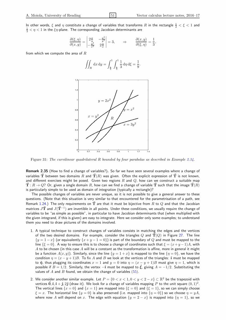
A. Moiola, University of Reading 51 Vector calculus lecture notes, 2016–17
In other words, ξ and η constitute a change of variables that transforms R in the rectangle 12 < ξ < 1 and
13 < η < 1 in the ξη-plane. The corresponding Jacobian determinants are
∂(ξ, η)
∂(x, y)=
∣∣∣∣∣2xy −x2
y2
− y2
x2 2 yx
∣∣∣∣∣ = 3, ⇒ ∂(x, y)
∂(ξ, η)=
1
3,
from which we compute the area of R
∫∫
R
dxdy =
∫ 1
12
∫ 1
13
1
3dη dξ =
1
9.
0 0.2 0.4 0.6 0.8 1 1.2 1.40
0.2
0.4
0.6
0.8
1
1.2
1.4
y = x2
y = 2x2
x = y2
x = 3y2
R
Figure 31: The curvilinear quadrilateral R bounded by four parabolas as described in Example 2.34.
Remark 2.35 (How to find a change of variables?). So far we have seen several examples where a change of
variables ~T between two domains R and ~T(R) was given. Often the explicit expression of ~T is not known,and different exercises might be posed. Given two regions R and Q, how can we construct a suitable map~T : R → Q? Or, given a single domain R, how can we find a change of variable ~T such that the image ~T(R)is particularly simple to be used as domain of integration (typically a rectangle)?
The possible changes of variables are never unique, so it is not possible to give a general answer to thesequestions. (Note that this situation is very similar to that encountered for the parametrisation of a path, see
Remark 1.24.) The only requirements on ~T are that it must be bijective from R to Q and that the Jacobian
matrices J ~T and J(~T−1) are invertible in all points. Under these conditions, we usually require the change ofvariables to be “as simple as possible”, in particular to have Jacobian determinants that (when multiplied withthe given integrand, if this is given) are easy to integrate. Here we consider only some examples; to understandthem you need to draw pictures of the domains involved.
1. A typical technique to construct changes of variables consists in matching the edges and the verticesof the two desired domains. For example, consider the triangles Q and ~T(Q) in Figure 27. The liney = 1− x (or equivalently x+ y− 1 = 0) is part of the boundary of Q and must be mapped to theline ξ = 0. A way to ensure this is to choose a change of coordinates such that ξ = (x+ y− 1)A, withA to be chosen (in this case A will be a constant as the transformation is affine, more in general it mightbe a function A(x, y)). Similarly, since the line y = 1+ x is mapped to the line η = 0, we have thecondition η = (x− y+1)B. To fix A and B we look at the vertices of the triangles: ı must be mappedto η, thus plugging its coordinates x = 1 and y = 0 into η = (x − y + 1)B must give η = 1, which ispossible if B = 1/2. Similarly, the vertex −ı must be mapped to ξ, giving A = −1/2. Substituting thevalues of A and B found, we obtain the change of variables (55).
2. We consider another similar example. Let P = 0 < x < 1, 0 < y < 2− x ⊂ R2 be the trapezoid withvertices ~0, ı, ı+ , 2 (draw it). We look for a change of variables mapping P to the unit square (0, 1)2.The vertical lines x = 0 and x = 1 are mapped into ξ = 0 and ξ = 1, so we can simply chooseξ = x. The horizontal line y = 0 is also preserved (i.e. mapped into η = 0) so we choose η = yA,where now A will depend on x. The edge with equation y = 2 − x is mapped into η = 1, so we

A. Moiola, University of Reading 52 Vector calculus lecture notes, 2016–17
have 1 = η = yA = (2− x)A so A(x) = 1/(2− x) and the transformation, with its inverse, reads20
ξ = x,
η = y/(2− x),
x = ξ,
y = (2− ξ)η.
3. If R has four edges, denoted ΓS ,ΓE ,ΓN and ΓW , we can look for two two-dimensional continuous fieldsξ, η : R→ R2 such that each edge corresponds to a level set:
ΓS = η = cS, ΓE = ξ = cE, ΓN = η = cN, ΓW = ξ = cW ,
where cS < cN and cW < cE are real numbers. Then, if the map ξ(x, y)ξ + η(x, y)η is injective on R,it is a change of variables with image the rectangle (cW , cE)× (cS , cN ). A prototypical case is describedin Example 2.34.
4. If a domain is x- or y-simple (see (52)), it can be mapped to a rectangle with the procedure describedin Example 2.33
5. If the domain has some circular symmetry, polar coordinates can be used, as described in Section 2.3.1.
Another instructive example is in Exercise 2.36.
Exercise 2.36 (Assignment 3, MA2VC 2013). Consider the unit square S = (0, 1)2 = xı + y, 0 < x <1, 0 < y < 1 and the triangle T = ξξ + ηη, 0 < ξ < η < 1 with vertices ~0, η and ξ + η.
(i) Find a simple (bijective) change of variables (x, y) 7→ (ξ, η) that maps S into T .Hint: consider a polynomial transformation that deforms the x variable only.(ii) Use the change of variables you found to compute
∫∫T
ξη dξ dη.
2.2.3 Triple integrals
All what we have said about double integrals immediately extends to triple integrals, namely integrals onthree-dimensional domains. It is not possible to have an easy geometrical interpretation of triple integralsas that in Figure 25 for double integrals. The volume integral of a positive field f on a domain D may beunderstood as total mass of a body of shape D and density f .
As before, triple integrals can be computed as iterated integrals. For instance, consider a “z-simple”domain D ⊂ R3, defined as
D =xı + y+ zk s. t. xL < x < xR, a(x) < y < b(x), α(x, y) < z < β(x, y)
for two real numbers xL and xR, two real functions a and b, and two scalar fields (in two variables) α andβ. Then, the integral in D of a scalar field f can be written as
∫∫∫
D
f(x, y, z) dxdy dz =
∫ xR
xL
(∫ b(x)
a(x)
(∫ β(x,y)
α(x,y)
f(x, y, z) dz
)dy
)dx. (62)
The infinitesimal volume element is defined as dV = dxdy dz.
~0
ı
k
Figure 32: The tetrahedron with vertices ~0, ı, and k.
For example, the tetrahedron B with vertices ~0, ı, and k depicted in Figure 32 can be written as
B =xı + y+ zk s. t. 0 < x < 1, 0 < y < 1− x, 0 < z < 1− x− y
.
20You can visualise this change of coordinates in Matlab/Octave using the function VCplotter.m (available on the courseweb page), with the command: VCplotter(6, @(x,y) x, @(x,y) y*(2-x),0,1,0,1);
A. Moiola, University of Reading 53 Vector calculus lecture notes, 2016–17
In this example, xL = 0, xR = 1, a(x) = 0, b(x) = 1− x, α(x, y) = 0 and β(x, y) = 1− x− y.The change of variable formula (57) extends to three dimensions in a straightforward fashion. If the
transformation ~T : D → ~T(D) has components
ξ(x, y, z), η(x, y, z), σ(x, y, z),
and its Jacobian determinant is
∂(ξ, η, σ)
∂(x, y, z)= det(J ~T) =
∣∣∣∣∣∣∣∣∣∣∣∣
∂ξ
∂x
∂ξ
∂y
∂ξ
∂z∂η
∂x
∂η
∂y
∂η
∂z∂σ
∂x
∂σ
∂y
∂σ
∂z
∣∣∣∣∣∣∣∣∣∣∣∣
,
then the change of variable formula reads
∫∫∫
D
f(x, y, z) dxdy dz =
∫
~T(D)
f(x(ξ, η, σ), y(ξ, η, σ), z(ξ, η, σ)
)∣∣∣∣∂(x, y, z)
∂(ξ, η, σ)
∣∣∣∣dξ dη dσ, (63)
for any scalar field f defined in D.Returning to the previous example, the tetrahedron B is the image of the unit cube 0 < x, y, z < 1
under the transformation ~T with components
ξ = (1− z)(1− y)x, η = (1 − z)y, σ = z. (64)
The corresponding Jacobian is
∂(ξ, η, σ)
∂(x, y, z)= det(J ~T) =
∣∣∣∣∣∣
(1− z)(1− y) −(1− z)x −(1− y)x0 (1− z) −y0 0 1
∣∣∣∣∣∣= (1 − y)(1− z)2.
In order to demonstrate the formulas of this section, we compute the volume of the tetrahedron Bintegrating the constant 1 first with the iterated integral (62) and then with the change of variables (63):
Vol(B) =
∫∫∫
B
1 dxdy dz
(62)=
∫ 1
0
(∫ 1−x
0
(∫ 1−x−y
0
1 dz
)dy
)dx
=
∫ 1
0
(∫ 1−x
0
(1− x− y
)dy
)dx =
∫ 1
0
1
2(1− x)2 dx =
1
2
(x− x2 +
1
3x3)∣∣∣∣
1
0
=1
6,
Vol(B) =
∫∫∫
B
1 dξ dη dσ
(63)=
∫∫∫
~T−1(B)
∂(ξ, η, σ)
∂(x, y, z)dxdy dz
=
∫ 1
0
∫ 1
0
∫ 1
0
(1− y)(1− z)2 dxdy dz =
(∫ 1
0
dx
)(∫ 1
0
(1 − y) dy
)(∫ 1
0
(1− z)2 dz
)= 1
1
2
1
3=
1
6.
2.2.4 Surface integrals
There is another kind of integrals we have not encountered yet: we have seen integrals along curves, on flatsurfaces, and on volumes, what is still missing are integrals on curved surfaces. This section introducessurface integrals of scalar fields; Section 2.2.5 considers surface integrals of vector fields.
Comparison with scalar calculus 2.37. Surfaces might be thought as the two-dimensional generalisation ofpaths: as paths are “curvilinear segments”, surfaces are “curvilinear planar regions”. Intuitively, paths andsurfaces are one- and two-dimensional subsets of R3, respectively. As paths can be defined by two equationsin x, y and z, surfaces can be written with a single equation, e.g.
~r ∈ R3, x2 + y2 = 1, z = 0
is a path (the unit circle),
~r ∈ R3, x2 + y2 + z2 = 1
is a surface (the unit sphere).
However, we have seen in Section 2.1 that to compute integrals along a path Γ we need a parametrisation ~a,i.e. a bijective function mapping an interval to the path itself. Similarly, computing surface integrals will requirea parametrisation, which in this case will be a map (denoted ~X) from a planar region to the surface itself.

A. Moiola, University of Reading 54 Vector calculus lecture notes, 2016–17
We will consider surfaces satisfying the following definition.
Definition 2.38. We say that a set S ⊂ R3 is a parametric surface if there exist a two-dimensional openregion R ⊂ R2 and a continuous, injective vector field ~X : R → R3 such that S is the image of R under ~X, i.e.S = ~r ∈ R3 such that ~r = ~X(~p), for some ~p ∈ R. The field ~F is called parametrisation, or chart, of S.
We always tacitly assume that the field ~X is smooth. For a given (non-empty) surface S there exist
infinitely many different parametrisations ~X. The assumption that ~X be injective (i.e. if ~p, ~q ∈ R are
different ~p 6= ~q, then they have different images ~X(~p) 6= ~X(~q)) is needed to avoid self-intersections of S.
Remark 2.39. The three components X1, X2 and X3 of the field ~X are the components of the points ~r ∈ S,thus to avoid confusion we will usually denote the two input variables (living in R ⊂ R2) of ~X with the letters
u and w instead of x and y. So we will write ~X(u,w) = ~X(uu+ww) = X1(u,w)ı+X2(u,w)+X3(u,w)k.The scalars u and w play a similar role to t for curves, but being two we can not interpret them as time.
Example 2.40. The graph of the scalar field in two variables f = x2−y2 in Figure 5 is a surface and is definedby the equation S = ~r ∈ R3, z = x2 − y2. Thus a chart for it is ~X(u,w) = uı + w + (u2 − w2)k. Ifwe want to consider the whole graph of f as an unbounded surface we take the region R as the whole of R2.If we want to define S to be only the bounded portion shown in Figure 5, we choose the region R to be thesquare (−2, 2)× (−2, 2) = |u|, |w| < 2. If we want S to look like a Pringles crisp we choose a circular regionR = u2 + w2 < 1.
Example 2.41. The unit sphere x2 + y2 + z2 = 1 is clearly a surface, but can not be written in the simpleframework of Definition 2.38. However the “punctured unit sphere” x2 + y2 + z2 = 1, z 6= 1 i.e. the unit
sphere with the north pole point removed is a parametric surface. The chart ~X : R2 → S is the famous“stereographic projection” (see Figure 33):
~X(u,w) =uı+ w+
(u2
4 + w2
4 − 1)k
1 + u2
4 + w2
4
. (65)
Exercise 2.42. Show that the stereographic projection (65) maps R = R2 into the punctured unit sphere.
Compute the inverse map ~X−1 : S → R2.
x
k
~0
(u,w)
~X(u,w)
Figure 33: A representation of the stereographic projection ~X : R2 → S in (65), S being the punctured unitsphere. The figure shows the vertical section y = 0. We identify the uw-plane with the horizontal planez = −1 (the lower horizontal line in the figure). A point ~p = uu+ ww = uı + w − k in this plane is
mapped by ~X into the intersection between the unit sphere and the segment connecting ~p itself to the northpole k. The point u = 0, w = 0 is mapped to the south pole −k, the points in the circle u2 +w2 = 2 are
mapped to the equator x2 + y2 = 1, z = 0, and the point “at infinity” is mapped to the north pole ~k.
Exercise 2.43. Fix two numbers 0 < b < a. Try to draw the surface defined by the chart
~X(u,w) = (a+ b cosw) cos uı+ (a+ b cosw) sinu+ b sinwk − π < u < π, −π < w < π.
From Example 2.41 and Exercise 2.43 we see that some simple surfaces, such as the sphere, cannot bewritten as parametric surfaces according to Definition 2.38. A more general definition could be given toinclude these surfaces but it is beyond the scope of this course. However, Example 2.40 suggests that thisdefinition includes a very important class of surfaces, those defined as graphs of fields in two variables.We describe them in the next very important remark.

A. Moiola, University of Reading 55 Vector calculus lecture notes, 2016–17
Remark 2.44. Given a region R ⊂ R2 and a planar scalar field g : R → R, the graph of g is the surface
Sg =~r ∈ R3 s.t. xı + y ∈ R, z = g(x, y)
⊂ R3. (66)
A chart for Sg is given by the vector field ~Xg(u,w) = uı+w+ g(u,w)k, which is defined on R. In this case,we can identify u with x and w with y. The main property of a graph surface is that for each point xı + yin the planar region R there is exactly one point in S that lies in the vertical line through xı+ y, namely thepoint xı+ y+ h(x, y)k.
A graph surface can be written in brief as Sg = z = g(x, y), meaning that Sg is the set of the points~r whose coordinates x, y and z are solutions of the equation in braces. Some examples of graph surfaces arethe paraboloid of revolution z = x2 + y2 (e.g. a satellite dish is a portion of it), the hyperbolic paraboloid
z = x2−y2 of Example 2.40, the upper half sphere z =√1− x2 − y2, x2+y2 < 1. The entire sphere is
not a graph, since to each point xı+ y in the plane, with x2 + y2 < 1, correspond two different points on thesphere; on the other hand the sphere can be written as union of two graphs, the north and south hemispheres.
Given a surface S defined by the chart ~X and the region R, and given a point ~r0 = ~X(u0, w0) ∈ S, the
partial derivatives of the vector field ~F, i.e. ∂~F∂u (u0, w0) and ∂~F
∂w (u0, w0) represent two tangent vectors
to S. Assuming that the tangent vectors ∂~F∂u and ∂~F
∂w are linearly independent, it follows that their vector
product ∂ ~X∂u × ∂~X
∂w is perpendicular to S.
Exercise 2.45. Consider the surface graph Sg for the field g(x, y) = 16xy(1 − x)(1 − y) defined inR = (0, 1)2 = xı+ y, 0 < x, y < 1. Draw Sg and compute its tangent vector fields.
⋆ Remark 2.46 (Tangent plane to a surface). Given a parametric surface S and a point ~r0 = ~X(u0, w0) ∈ S,the plane
TS~r0 =~X(u0, w0) + u
∂ ~X
∂u(u0, w0) + w
∂ ~X
∂w(u0, w0), for all u,w ∈ R
is called the tangent plane to S in ~r0. When we say that a vector is perpendicular to a surface S in a point~r0, what we actually mean is that it is perpendicular to TS~r0. If ~r0 is placed on a vertex or an edge of S, then~X is not differentiable at u0u+ w0w and no tangent plane nor perpendicular vectors can be defined.
For a graph surface Sg as in (66), using the chart ~Xg(u,w) = uı+w+ g(u,w)k, we see that the tangent
vectors are∂ ~Xg
∂u = ı+ ∂g∂u k and
∂~Xg
∂w = + ∂g∂w k. Thus, renaming x = u+ u0, y = w+w0, x0 = u0, y0 = w0,
the tangent plane can be written as
xı+ y+
(g(x0, y0) + ~∇g(x0, y0) ·
((x− x0)ı + (y − y0)
))k, for all x, y ∈ R
.
This coincides with the formula already obtained in Remark 1.40.
We now have all the tools needed to compute integrals over surfaces. Given a scalar field f defined ona parametric surface S, given by the chart ~X and the region R, the integral of f over S is
∫∫
S
f dS =
∫∫
R
f(~X)
∣∣∣∣∣∂ ~X
∂u× ∂ ~X
∂w
∣∣∣∣∣ dA =
∫∫
R
f(~X(u,w)
)∣∣∣∣∣∂ ~X
∂u(u,w)× ∂ ~X
∂w(u,w)
∣∣∣∣∣ du dw. (67)
where the integral at the right-hand side is a double integral on the (flat) region R as those studied inSection 2.2.1. Note that we used the symbol
∫∫, since the domain of integration is two-dimensional.
The symbol dS denotes the infinitesimal area element on S; it is the “curvilinear analogue” of dA orthe “two-dimensional analogue” of ds. Formula (67) states that the ratio between the area element onS and that on the parametric region R equals the magnitude of the vector product between the partialderivatives of the chart.
The surface integral (67) is independent of the chart: if ~X : R→ S and ~Y : Q→ S are different charts
of the same surface S, then it is possible to prove21 that∫∫
R f(~X)|∂ ~X
∂u × ∂~X∂w | dA =
∫∫Q f(
~Y)|∂ ~Y∂u × ∂ ~Y
∂w | dA,thus the notation
∫∫S f dS is well-defined (recall Example 2.3 for path integrals).
We can easily specialise formula (68) to the case of a graph surface. If Sg is the graph of a field g as
in (66), the chart ~X(u,w) = uı+ w+ g(u,w)k has derivatives
∂ ~X
∂u= ı+
∂g
∂uk,
∂ ~X
∂w= +
∂g
∂wk, ⇒ ∂ ~X
∂u× ∂ ~X
∂w= −∂g
∂uı− ∂g
∂w+ k.
21This follows from the fact that ~Y−1 ~X : R → Q is a change of variables.

A. Moiola, University of Reading 56 Vector calculus lecture notes, 2016–17
Plugging this into the surface integral formula (67) and identifying u = x and w = y, we have that theintegral on Sg of a scalar field f can be computed as
∫∫
Sg
f dS =
∫∫
R
f
√1 + |~∇g|2 dA =
∫∫
R
f(x, y, g(x, y)
)√
1 +(∂g∂x
(x, y))2
+(∂g∂y
(x, y))2
dA, (68)
The area of a parametric surface (or of a graph) are computed by integrating the constant scalar fieldf = 1 (recall the basic properties of integrals in (40) and the path length formula (43)):
Area(S) =
∫∫
R
∣∣∣∣∣∂ ~X
∂u× ∂ ~X
∂w
∣∣∣∣∣ du dw, Area(Sg) =
∫∫
R
√1 + |~∇g|2 dxdy. (69)
Remark 2.47. The measure factor
√1 + |~∇g|2 in (68) should recall you the similar coefficient
√1 + (g′(t))2
we found in the computation of integrals along the graph of a real function in Example 2.5.
⋆ Remark 2.48 (Relation between change of variables and surface integrals). A two-dimensional change of
variables ~T : R → ~T(R) can be considered the chart of a “flat parametric surface” by identifying ~X = ~T,
u = ξ, w = ξ. Since X3 = 0, we have ∂ ~X∂u × ∂ ~X
∂w = (∂T1
∂ξ∂T2
∂η − ∂T2
∂ξ∂T1
∂η )k = ∂(x,y)∂(ξ,η) , so the change of variables
formula (57) is a special case of the surface integral formula (67). Thus a justification of the latter follows alongthe lines of Remark 2.32. (In particular formula (61) shows how the vector product enters the area element.)
Exercise 2.49. Compute the area of the parametric surface defined by the chart ~X(u,w) = (u + w)ı +(u− w) + k on the region R = (0, 1)2 = 0 < u,w < 1.
Exercise 2.50. Compute the area of the surface
S =~r ∈ R3, z =
2
3
(x
32 + y
32
), 0 < x < 1, 0 < y < 1
.
Exercise 2.51. (i) Compute the area of the parametric surface defined in Exercise 2.43. You can choosea = 2 and b = 1 for simplicity.
(ii) Compute the integral on S of the field f(~r) = (x2 + y2)−1/2.
We will examine other examples of surface integrals in the next sections.
2.2.5 Unit normal fields, orientations and fluxes (surface integrals of vector fields)
Remark 2.52 (Physical motivation for the definition of flux). Imagine a pipe containing a fluid which moves
with stationary (i.e. independent of time) velocity ~F(~r) at each point ~r. Denote by S a section of the pipe,
which we model as a surface. Given ~F and S, how can we compute the flux through the pipe, i.e. the volumeof fluid passing through the section S in a unit of time? This must be an integral, summing the contributionsfrom all portions of the section. Moreover, it must be independent of the tangential component of ~F on S,as particles moving tangentially do not cross the surface. We also need to be able to distinguish the amountof flux crossing S in one direction from that crossing it in the opposite direction, thus to distinguish the two“sides” of S. This situation motivates the following definitions.
(We consider for a moment general surfaces, even those not included in Definition 2.38.) For everypoint ~r on a smooth surface S, it is possible to define exactly two unit vectors nA and nB that areorthogonal to S in ~r. These two vectors are opposite to each other, i.e. nA = −nB, and they are calledunit normal vectors. If for every point ~r ∈ S we fix a unit normal vector n(~r) in a continuous fashion(i.e. n is a continuous unit normal vector field defined on S), then the pair (S, n) is called orientedsurface. Note that the pairs (S, n) and (S,−n) are two different oriented surfaces, even though theyoccupy the same portion of the space.22
Not all surfaces admit a continuous unit normal vector field, the most famous example of non-orientablesurface is the Mobius strip shown in Figure 34. On the other hand, the surfaces in the following threeimportant families admit an orientation.
22Oriented surfaces share many properties with the oriented paths seen in Section 2.1. Also in that case, a path Γ supportstwo different orientations, corresponding to travel directions, leading to two different oriented paths. In both cases, theorientation is important to integrate vector fields, while is not relevant for the integration of scalar fields; can you guess why?

A. Moiola, University of Reading 57 Vector calculus lecture notes, 2016–17
-0.4
-11
-0.2
-0.50.5
0
00
0.2
0.5
0.4
-0.5
1-1
1.5
Figure 34: The Mobius strip. This surface is not orientable: if we continuously move a unit normal vectoralong the surface, after one turn it will point in the direction opposite to the direction it started from. Youcan easily build a Mobius strip with a strip of paper.The chart ~X = (1 + w cos(u/2)) cosu ı + (1 + w cos(u/2)) sinu + w sin(u/2)k for 0 < u < 2π and−0.5 < w < 0.5 gives the Mobius strip without the the segment 0.5 < x < 1.5, y = z = 0 (in red in thefigure), corresponding to u = 0. Indeed, if we cut the surface along this segment, we cannot complete aturn along the surface itself and the surface obtained is orientable.
(i) If S is a parametric surface as in Definition 2.38 with chart ~X : R → S, then it is orientable withunit normal vector
n(~r) =
∂ ~X
∂u× ∂ ~X
∂w∣∣∣∣∣∂ ~X
∂u× ∂ ~X
∂w
∣∣∣∣∣
. (70)
A special case is when Sg is the graph of a two-dimensional scalar field g as in (66), then (70) reads
n(~r) =
−∂g∂x
ı− ∂g
∂y+ k
√
1 +
(∂g
∂x
)2
+
(∂g
∂y
)2. (71)
Since the z-component of n in this formula is positive, this is the unit normal that points upwards.
(ii) Another family of surfaces admitting a unit normal vector fields are the boundaries of three-dimensional domains. The boundary of a domain D ⊂ R3 is commonly denoted by ∂D and is asurface (if D is “smooth enough”). In this case, we usually fix the orientation on ∂D by choosingthe outward-pointing unit normal vector field.
(iii) If the surface S is the level surface of a smooth scalar field f satisfying ~∇f 6= ~0 near S (see
Section 1.2.1), then n = ~∇f/|~∇f | is an admissible unit normal field and (S, n) is an orientedsurface23. This is a consequence of Part 4 of Proposition 1.33. We have seen a special case of thissituation in Example 1.38. These surfaces are defined by the equation S = f(~r) = λ.
Note that if S is the graph of g as in item (i), then it is also the level set of the field f(x, y, z) = z−g(x, y),whose gradient is ~∇f = − ∂g
∂x ı−∂g∂y + k. So, the unit normal vector fields in (71) is a special case of both
(70) and of item (iii) of the list above.
23Can you imagine what happens if ~∇f = ~0?

A. Moiola, University of Reading 58 Vector calculus lecture notes, 2016–17
⋆ Remark 2.53 (Normal unit vectors on piecewise smooth surfaces). The situation is more complicated whenthe surface S is not smooth but only “piecewise smooth”, for instance is the boundary of a polyhedron. Inthis case it is not possible to define a continuous unit normal vector field. For instance, on the boundary∂C = max|x|, |y|, |z| = 1 of the unit cube C = max|x|, |y|, |z| ≤ 1, the outward-pointing unitnormal vectors on two faces meeting at an edge are orthogonal to each other, so when crossing the edge theysuddenly “jump”, i.e. they are not continuous. However, it is possible to give a precise definition of orientationalso in this case, formalising the idea that n stays on “the same side” of S (see [1, page 881]). In all practicalcases, with a bit of geometric intuition it should be clear how to define a normal field in such a way that itstays on the same side of the surface (and so it determines the surface orientation).
Given an oriented surface (S, n) and a vector field ~F defined on S we define the flux of ~F through
(S, n) as the value of the integral over S of the normal component of ~F:
flux of ~F through (S, n) :=
∫∫
S
~F · d~S :=
∫∫
S
~F · n dS. (72)
Note that the integrand ~F · n is nothing else than a scalar field defined on S, so the flux can be computedas a surface integral studied in Section 2.2.4.
Combining the integral formula (67) and the expression (70) of the unit normal vector, we immediately
obtain the formula for the flux of a vector field through a parametric surface S with chart ~X : R→ S:
∫∫
S
~F · d~S =
∫∫
R
~F ·(∂ ~X∂u
× ∂ ~X
∂w
)dA (73)
=
∫∫
R
~F(~X(u,w)
)·(∂ ~X∂u
(u,w)× ∂ ~X
∂w(u,w)
)du dw.
Similarly, on the graph surface (66) of g, the area element√
1 + ( ∂g∂x)2 + ( ∂g∂y )
2 in (68) and the denominator
in the unit normal (71) cancel each other and the integral in the flux (72) simplifies to24
∫∫
Sg
~F · d~S =
∫∫
R
(− F1
∂g
∂x− F2
∂g
∂y+ F3
)dA (74)
=
∫∫
R
(− F1
(x, y, g(x, y)
)∂g∂x
(x, y)− F2
(x, y, g(x, y)
)∂g∂y
(x, y) + F3
(x, y, g(x, y)
))dxdy.
If the surface is a domain boundary ∂D, the surface integral and the flux are often denoted by the symbols
∫∫
∂D
f dS and
∫∫
∂D
~F · d~S.
Remark 2.54. The flux∫∫
S~F · d~S measures “how much” of the vector field ~F crosses the surface S in the
direction given by n. If ~F is tangent to the surface in every point then the flux is zero.
Exercise 2.55. Compute the flux of the vector field ~F = ~r× ı = z− yk through the hyperbolic paraboloidS = z = x2 − y2, 0 < x, y < 1 (see Figure 5).
Exercise 2.56. Consider the graph surface Sg of Exercise 2.45 (i.e. g(x, y) = 16x(1 − x)y(1 − y) and
R = (0, 1)2). Let ~F = ı and ~G = xı be two vector fields. Equip Sg with the unit normal vector of (71) (you
do not need to compute n!). Compute the fluxes of ~F and ~G through Sg.Can you guess the value of one of this fluxes and the sign of the other before computing them?
Exercise 2.57. Compute the flux of the position vector ~F(~r) = ~r through the parametric surface ofExercise 2.43. You can assume again a = 2 and b = 1. Hint: the computations already done in Exercise 2.51might be helpful.
A surface S may have a boundary ∂S, which is the path of a curve. For instance, the boundary ofthe upper half sphere S = |~r| = 1, z ≥ 0 is the unit circle ∂S = xı + y, x2 + y2 = 1 (the equator),while the complete sphere |~r| = 1 has no boundary. The boundary of the open cylindrical surfaceC = x2 + y2 = 1, |z| < 1 is composed of the two circles ∂C = x2 + y2 = 1, z = ±1.
24Note that when we write, for example,∫∫
RF1
∂g∂x
dA what we actually mean is the integral over the region R of
F1(x, y, g(x, y)
) ∂g∂x
(x, y): the two dimensional field g (giving the shape of the surface S) is defined on R ⊂ R2, while
the three-dimensional field F1 is defined only on the surface S ⊂ R3, whose points can be written as xı+ y+ g(x, y)k.

A. Moiola, University of Reading 59 Vector calculus lecture notes, 2016–17
We have defined orientations for both paths and surfaces, we now relate the orientation of a surfacewith the that of its boundary. An oriented surface (S, n) “induces an orientation” on its boundary,i.e. there is a standard way of choosing one of the two possible path orientations of its boundary. GivenS and n, the induced path orientation on ∂S is the travel direction such that walking along∂S, on the side of S defined by n, we leave S itself on our left. This definition may be veryconfusing, try to visualise it with a concrete example, e.g. using a sheet of paper as model for a surface;see also Figure 35.
y
z
x
n
S ∂S
Figure 35: The relation between the orientation of an oriented surface, given by the continuous unitnormal field n, and the orientation of the boundary ∂S (the direction of travel along the path). Imagineto walk along the path ∂S, according to the arrows, and staying on the same side of the vector n (i.e.above the surface). Then S is always at our left. So the path-orientation of ∂S is that one induced by thesurface-orientation of S.
⋆ Remark 2.58. In Section 2 we have defined several different kinds of integrals. Single, double and tripleintegrals, denoted by the differentials dt, dA, dV , are standard or iterated integrals computed on “flat” (1-,
2-, or 3-dimensional) domains. Line and surface integrals denoted by the differentials ds, d~r, dS, d~S requirea parametrisation describing the shape of the domain, which is a curve or a surface and might be not flat.
⋆ Remark 2.59 (The boundary of a boundary). Note that if the surface S is the boundary of a volumeD ⊂ R3, i.e. S = ∂D, then S has empty boundary ∂S = ∅. You may find this fact stated as ∂2 = ∅, wherethe symbol “∂” stands for the action “taking the boundary”. Try to think at some geometric examples.
Warning: do not mix up the different objects, the boundary ∂D of a volume D is a surface (the skin of anapple), the boundary ∂S of a surface S is a path (the edge of a sheet, the border of a country).
⋆ Remark 2.60 (Boundaries and derivatives). Why are boundaries and derivatives denoted by the samesymbol “∂”? This notation comes from the profound theory of differential forms, however, we can see thatthese two apparently unrelated objects share some properties. A fundamental property of derivatives is theproduct rule: (fg)′ = f ′g + fg′ for scalar functions, or ~∇(fg) = (~∇f)g + f ~∇g for scalar fields, (28).Now consider the Cartesian product of the two segments [a, b] ⊂ R and [c, d] ⊂ R, namely the rectangleR = [a, b] × [c, d] = xı + y, a ≤ x ≤ b, c ≤ y ≤ d. Its boundary is the union of four edges [a, b] × c,[a, b]×d, a×[c, d], and b×[c, d]. The boundaries of the segments are ∂[a, b] = a, b and ∂[c, d] = c, d.Therefore we can write
∂([a, b]× [c, d]
)=([a, b]× c
)∪([a, b]× d
)∪(a × [c, d]
)∪(b × [c, d]
)
=([a, b]× c, d
)∪(a, b × [c, d]
)
=([a, b]× ∂[c, d]
)∪(∂[a, b]× [c, d]
)
which closely resembles the product rule for derivatives. Here the Cartesian product (×) plays the role of multi-plication, the set union (∪) that of addition and the action “take the boundary” plays the role of differentiation.A similar formula holds true for much more general domains; try to see what is the boundary of the Cartesianproduct of a circle and a segments, two circles, or a planar domain and a segment. If you are curious aboutthis analogy take a look at the post http://mathoverflow.net/questions/46252.

A. Moiola, University of Reading 60 Vector calculus lecture notes, 2016–17
2.3 Special coordinate systems
Among the possible changes of coordinates described in Section 2.2.2, some are particularly important.Polar coordinates are used for two-dimensional problems with some circular symmetry around a centre,while cylindrical and spherical coordinates are used in three dimensions. Several other special (more com-plicated) coordinate systems exist, we do not consider them here. You should remember polar coordinatesfrom page 31 of handout 5 of last year calculus class. In Table 2 at the end of this section we summarisethe most important facts to keep in mind for the three system of coordinates studied here25.
These systems of coordinates are meant to simplify computations in problems with some geometricalsymmetry. For example, cylindrical coordinates are related to axial symmetry and spherical coordinatesto central symmetry. So the former system will be useful to compute triple integrals on cylinders andshapes like barrels or funnels; the latter for shapes like spheres or portions of them. On the other hand,if you try to use these systems on different geometries, like tetrahedra or parallelepipeds, you will end upwith horrible computations, as they are not meant to be used in these cases.
In table 4 in Section G at the end of these notes, you can find a list of exercises from the textbookwhere you can combine special coordinate systems with the techniques learned in the previous sections,such as line integrals, multiple integrals, potentials.
2.3.1 Polar coordinates
The polar coordinates r and θ are defined by the relations26
x = r cos θ,
y = r sin θ,
r =
√x2 + y2,
θ = tan−1 y
x.
(75)
The xy-plane R2 is mapped by this transformation into the strip r ≥ 0,−π < θ ≤ π. Given a pointxı+ y, the value of r is the distance from the origin, while the value of θ is the (signed) angular distancebetween the direction ı of the x axis and the direction of the point itself. If r = 0, i.e. for the origin ofthe Cartesian axes, the angular coordinate θ is not defined.
xθ = 0
y θ = π/2
r = 1r = 2
~rr
θ
ı
rθθ = 3
4π
θ = − 14π
r cos θ
r sin θ
r
θ
π
−π
~0
Figure 36: Left: the polar coordinate system.Right: the change of variables (x, y) 7→ (r, θ) maps the punctured plane R2 \ ~0 to the semi-infinite strip(0,∞)× (−π, π] in the rθ-plane.
We compute the Jacobian of the direct and the inverse transformations:(
∂x∂r
∂x∂θ
∂y∂r
∂y∂θ
)=
(cos θ −r sin θsin θ r cos θ
),
25The page http://en.wikipedia.org/wiki/Del_in_cylindrical_and_spherical_coordinates contains a useful sum-mary of these and many other identities and formulas (in 3D only). However, the notation used there is completely differentfrom that we have chosen in this notes: to compare those formulas with ours, r and ρ must be exchanged with each otherand similarly θ and φ! (See also footnote 29.) Our notation is chosen to be consistent with that of [1, Section 10.6].
26Here we are being quite sloppy. The “inverse” of the tangent function is usually called arctan and takes values in (−π2
π2).
Here tan−1 yx
is meant to be equal to arctan yx
only when x > 0 and to take values in (−π, π2] ∪ [π
2, π] otherwise. For the
exact definition, see http://en.wikipedia.org/wiki/Atan2. However, θ(x, y) can be easily computed “visually” as the angledetermined by the point xı+ y. E.g. if x > 0, y > 0, then xı+ y is in the first quadrant so θ belongs to the interval (0, π
2);
if x = −x < 0, y = −y < 0 then xı+ y belongs to the third quadrant and θ must be in the interval (−π,−π2), even if y
x= y
x
and arctan yx= arctan y
x.

A. Moiola, University of Reading 61 Vector calculus lecture notes, 2016–17
(∂r∂x
∂r∂y
∂θ∂x
∂θ∂y
)=
(∂x∂r
∂x∂θ
∂y∂r
∂y∂θ
)−1
=1
r
(r cos θ r sin θ− sin θ cos θ
)=
(xr
yr
− yr2
xr2
). (76)
(The second matrix can also be calculated directly using ∂(tan−1 t)∂t = 1
1+t2 .) The Jacobian determinantsare immediately computed as
∂(x, y)
∂(r, θ)= r(cos2 θ + sin2 θ) = r,
∂(r, θ)
∂(x, y)=
1
r=
1√x2 + y2
. (77)
Therefore, the infinitesimal area element in polar coordinates is
dA = dxdy = r dr dθ.
Example 2.61 (Area of the disc). As a simple application of the polar coordinate system, we compute thearea of the disc of radius a > 0 centred at the origin, i.e. Q = xı+ y s.t. x2 + y2 < a:
Area(Q) =
∫∫
Q
dxdy =
∫ a
0
∫ π
−π
r dθ dr =
∫ a
0
2πr dr = 2πr2
2
∣∣∣∣a
0
= πa2,
which agrees with the formula we know from elementary geometry.
In the “punctured plane” R2 \ ~0, we define two vector fields r and θ of unit magnitude:
r(x, y) = cos θı+ sin θ =x√
x2 + y2ı+
y√x2 + y2
=~r
|~r| , ⇒ ı(r, θ) = cos θr − sin θθ,
θ(x, y) = − sin θı + cos θ = − y√x2 + y2
ı+x√
x2 + y2, (r, θ) = sin θr + cos θθ.
(78)
In every point ~r 6= ~0 the two unit vectors r and θ are orthogonal one another and point in the direction ofincrease of the radial coordinate r and of the angular one θ, respectively; see Figure 36. In other words, rpoints away from the origin and θ points in the anti-clockwise direction. Using (78) every planar vectorfield defined in R2 \ ~0 can be expanded in r and θ:
~F = F1ı+ F2 = (cos θF1 + sin θF2)r + (− sin θF1 + cos θF2)θ = (~F · r)r + (~F · θ)θ.
Example 2.62 (Curves in polar coordinates and area of domains delimited by polar graphs). If the path of acurve ~a can be expressed in the form r = g(θ) for some positive function g, it is sometimes called a “polargraph”. In this kind of curves, the magnitude is function of the angle and the path can be seen as the graphof the function g in the rθ-plane. In this case we can choose t = θ and write ~a(t) = g(t)(cos tı + sin t) for−π < t ≤ π. For example, a circle of radius a can be written as r = a, i.e. the function g has constant valuea, thus we find the usual parametrisation ~a(t) = a(cos tı+ sin t).27
The domain R delimited by the curve ~a is “r-simple” in the rθ-plane (compare with the definition ofy-simple domain in (52)):
R =~r = xı + y ∈ R2, s.t.
√x2 + y2 < g
(θ(x, y)
)
=~r = r cos θı+ r sin θ ∈ R2, s.t. − π < θ ≤ π, 0 ≤ r < g(θ)
.
R is called “star-shaped region”28 and its area can be computed as
Area(R) =
∫∫
R
dxdy =
∫ π
−π
(∫ g(θ)
0
r dr
)dθ =
∫ π
−π
1
2r2∣∣∣∣g(θ)
0
dθ =1
2
∫ π
−π
g2(θ) dθ. (79)
For example, we compute the area of the domain delimited by the “propeller” curve r = (2 + cos 3θ)depicted in left plot of Figure 37: using cos2 t = 1
2 (t+ sin t cos t)′,
Area(R) =1
2
∫ π
−π
(2 + cos 3θ
)2dθ =
(2θ +
θ
4+
sin 3θ cos 3θ
12+
2
3sin 3θ
)∣∣∣∣π
−π
=9
2π.
27The “clover” curve ~c(t) = (cos 3t)(cos t)ı+(cos 3t)(sin t) in Figure 8 might be written in polar form as r = cos 3θ. Notethat here we are allowing negative values for the radial component! What does it mean? Compare with the curve plot.
28We have already defined star-shaped domains in Section 2.1.3, can you see the relation between the two definitions?

A. Moiola, University of Reading 62 Vector calculus lecture notes, 2016–17
(We can deduce from this computation that the area delimited by r = (2 + cosnθ) is independent of n ∈ N,i.e. all the “flower” domains in the centre plot of Figure 37 have the same area.) The path of the curver = (2 + cos 3θ) in the rθ-plane is the wave in the right plot of Figure 36.
We can also compute the area of more complicated shapes, for instance the domain between the two spiralsr = θ and r = 2θ (with 0 < θ < 2π) in the right plot of Figure 37:
∫ 2π
0
(∫ 2θ
θ
r dr
)dθ =
∫ 2π
0
1
2
(4θ2 − θ2
)dθ =
(2π)3
2= 4π3 ≈ 124.
2
4
30
210
60
240
90
270
120
300
150
330
180 0
2
4
30
210
60
240
90
270
120
300
150
330
180 0
2
4
30
210
60
240
90
270
120
300
150
330
180 0
2
4
30
210
60
240
90
270
120
300
150
330
180 0
10
20
30
210
60
240
90
270
120
300
150
330
180 0
Figure 37: The polar graph r = (2 + cosnθ) for n = 3 (left), n = 2 (upper centre), n = 7 (centre centre),n = 12 (lower centre). As seen in Example 2.62, they all have the same area. In the right plot, the twospirals r = θ and r = 2θ (with 0 < θ < 2π). These curves can be plotted with Matlab’s command polar.
⋆ Remark 2.63. Any scalar field in two variables f(x, y) can be expressed in polar coordinates as F (r, θ) =f(r cos θ, r sin θ). Here F is a function of two variables (as f) which represents the field f but has a differentfunctional expression (we have already used this fact several times without spelling it out). The gradient andthe Laplacian of f can be computed in polar coordinates using the chain rule:
~∇f(x, y) = ∂f(x, y)
∂xı+
∂f(x, y)
∂y
=∂F(r(x, y), θ(x, y)
)
∂xı+
∂F(r(x, y), θ(x, y)
)
∂y
=
(∂F
∂r
∂r
∂x+∂F
∂θ
∂θ
∂x
)ı+
(∂F
∂r
∂r
∂y+∂F
∂θ
∂θ
∂y
) (chain rule (38))
=∂F
∂r
(∂r
∂xı+
∂r
∂y
)+∂F
∂θ
(∂θ
∂xı+
∂θ
∂y
)
(76)=
∂F
∂r
(x
rı+
y
r
)+∂F
∂θ
(−yr2
ı+x
r2
)(78)=
∂F
∂rr +
1
r
∂F
∂θθ = ~∇F (r, θ). (80)
Thus, whenever we have a scalar field F expressed in polar coordinates, we can compute its gradient usingformula (80) (do not forget the 1
r factor!) without the need of transforming the field in Cartesian coordinates.
2.3.2 Cylindrical coordinates
There are two possible extensions of polar coordinates to three dimensions. The first one is used to treatproblems with some axial, or cylindrical, symmetry. By convention, the axis of symmetry is fixed to bethe axis z. The cylindrical coordinate r, θ and z corresponds to the polar coordinates r, θ in the xy-planeand the height z above this plane:
x = r cos θ,
y = r sin θ,
z = z,
r =√x2 + y2,
θ = tan−1 y
x,
z = z,
r ≥ 0,−π < θ ≤ π,
z ∈ R.(81)

A. Moiola, University of Reading 63 Vector calculus lecture notes, 2016–17
Proceeding as in (77), it is immediate to verify that the Jacobian determinants and the infinitesimalvolume element are
∂(x, y, z)
∂(r, θ, z)= r,
∂(r, θ, z)
∂(x, y, z)=
1
r, dV = dxdy dz = r dr dθ dz. (82)
This can be used to compute the volume of the solids of revolution
Dg =~r ∈ R3 s.t. zbot < z < ztop, r < g(z)
, (83)
where g : (zbot, ztop) → R is a non-negative function, as
Vol(Dg) =
∫∫∫
Dg
dV =
∫ ztop
zbot
(∫ π
−π
(∫ g(z)
0
r dr)dθ
)dz=
∫ ztop
zbot
(∫ π
−π
g2(z)
2dθ
)dz = π
∫ ztop
zbot
g2(z) dz.
(84)
Example 2.64 (Volume of solids of revolution). Compute the volume of the “pint” domain E in Figure 38:E =
~r ∈ R3 s.t. 0 < z < 1, r < 1
3 + 12z
2 − 13z
3.
Vol(E)(84)= π
∫ 1
0
(1
3+
1
2z2 − 1
3z3)2
dz = π
∫ 1
0
(1
9+
1
4z4 +
1
9z6 +
1
3z2 − 2
9z3 − 1
3z5)dz
= π
(1
9+
1
20+
1
63+
1
9− 1
18− 1
18
)=
223
1260≈ 0.177.
x
y
z
~r
r
z
θ
Figure 38: The domains described in Examples 2.64, 2.65 and Exercise 2.66: the pint E (left), the ellipsoidx2 + y2 + 4z2 < 1 (upper centre), the rugby ball B (lower centre) and the funnel F (right).
Exercise 2.65 (Volume of the ellipsoid). Compute the volume of the “oblate ellipsoid of revolution” bounded
by the surface x2 + y2 + z2
c2 = 1, for a real number c > 0.
Exercise 2.66. Calculate the volume of the rugby ball B and the (infinite) funnel F in Figure 38:
B =~r ∈ R3 s.t. − 1 < z < 1, r < 1− z2
, F =
~r ∈ R3 s.t. −∞ < z < 0, r < ez
.
Exercise 2.67. Cylindrical coordinates can also be used to deal with domains which are not solids ofrevolution. Can you draw the shape of D =
~r ∈ R3 s.t. − π
2 < z < π2 , r < (cos z)(2 + sin 3θ)
? Can you
compute its volume? You need to derive a slightly more general formula than (84) (compare with formula (79)for the area of polar graphs).
Exercise 2.68 (Triple integrals on a cone). Consider the cone C =~r ∈ R3 s.t. 0 < z < 1, r < z
. Verify
the following computations:∫∫∫
C
z dV =π
4,
∫∫∫
C
xdV = 0,
∫∫∫
C
(x2 + y2 + z2) dV =3π
10.
(The domain is easily defined in cylindrical coordinates, while the last two integrands are defined in Cartesiancoordinates, figure out how to deal with this fact.) Prove that, for any function g : (0, 1) → R,
∫∫∫
C
g(z) dV = π
∫ 1
0
g(z)z2 dz.

A. Moiola, University of Reading 64 Vector calculus lecture notes, 2016–17
⋆ Remark 2.69. As we did in (78) for the polar coordinates, also for the cylindrical system we can computethe vector fields with unit length lying in the direction of increase of the three coordinates:
r(x, y, z) =x√
x2 + y2ı +
y√x2 + y2
, ı = cos θr − sin θθ,
θ(x, y, z) = − y√x2 + y2
ı+x√
x2 + y2, = sin θr + cos θθ,
z(x, y, z) = k, k = z.
(85)
⋆ Remark 2.70 (Vector differential operators in cylindrical coordinates). As we did in equation (80) forpolar coordinates, we can compute the gradient of a scalar field f expressed in cylindrical coordinates. Sincewe are now considering a three-dimensional space, we also compute divergence and curl of a vector field~G = Grr + Gθθ + Gzz. We only write the final results (they can be derived from (81), (85) and the chainrule, but the computation are quite complicated):
~∇f(r, θ, z) = ∂f
∂rr +
1
r
∂f
∂θθ +
∂f
∂zz,
~∇ · ~G(r, θ, z) =1
r
∂(rGr)
∂r+
1
r
∂Fθ
∂θ+∂Fz
∂z=∂Gr
∂r+
1
rGr +
1
r
∂Fθ
∂θ+∂Fz
∂z, (86)
~∇× ~G(r, θ, z) =(1r
∂Fz
∂θ− ∂Fθ
∂z
)r +
(∂Fr
∂z− ∂Fz
∂r
)θ +
(∂Fθ
∂r+
1
rFθ −
1
r
∂Fr
∂θ
)z.
Exercise 2.71. Consider the vector field ~F = −yı+ x + k. Show that in cylindrical coordinates it reads~F = rθ + z. Use (86) to prove that ~F is solenoidal. This might be the field that gave the name to all
solenoidal fields: the streamlines of ~F are the helices (see Figure 8), which have the shape of a “solenoid” usedin electromagnetism (although Wikipedia suggests a different origin of the name).
Example 2.72 (Surface integrals in cylindrical coordinates). Polar and cylindrical coordinates can be used tocompute surface integrals. Consider the conic surface of unit radius and unit height (written in Cartesian andcylindrical coordinates):
S =~r ∈ R3, z =
√x2 + y2, x2 + y2 < 1
=~r ∈ R3, z = r, r < 1
.
(Note that S is part of boundary of the cone C in Exercise 2.68.) The surface S is the graph of the two-dimensional field g(r, θ) = r defined on the unit disc Q = ~r ∈ R3, r < 1. Thus, its area can be computedusing the graph surface integral formula (68), choosing f = 1. We also exploit the fact that the gradient of
g =√x2 + y2 = r satisfies ~∇g = ∂r
∂r r = r, when written in polar coordinates, see (80), so it has length one.We obtain:
Area(S)(68)=
∫∫
Q
1
√1 + |~∇g|2 dA =
∫ π
−π
∫ 1
0
√1 + 1 r dr dθ = 2π
√2
∫ 1
0
r dr = π√2 ≈ 4.443,
where in the second equality we used |~∇g| = |r| = 1.
2.3.3 Spherical coordinates
In order to deal with three-dimensional situations involving a centre of symmetry, we introduce thespherical coordinate system. The three coordinates, denoted by ρ, φ and θ, are called radius, colatitudeand longitude (or azimuth), respectively29. (The latitude commonly used in geography corresponds toπ2 − φ, hence the name colatitude.) For a point ~r, the radius ρ ≥ 0 is its distance from the origin (the
magnitude of ~r); the colatitude 0 ≤ φ ≤ π is the angle between the direction of ~r and the unit vector kon the axis z; the longitude −π < θ ≤ π is the polar angle of the projection of ~r on the xy-plane. Informulas:30
ρ = |~r| =√x2 + y2 + z2,
φ = arccos zρ = arccos z√
x2+y2+z2,
θ = tan−1 yx ,
x = ρ sinφ cos θ,
y = ρ sinφ sin θ,
z = ρ cosφ,
ρ ≥ 0,0 ≤ φ ≤ π,−π < θ ≤ π.
(87)
29We assign to colatitude and longitude the same symbols used in the textbook (see [1, Page 598]). However, in manyother references, the symbols θ and φ are swapped, e.g. in Calvin Smith’s “vector calculus primer” you might have used.According to http://en.wikipedia.org/wiki/Spherical_coordinates, the first notation is more common in mathematicsand the second in physics. Different books, pages of Wikipedia and websites use different conventions: this might be acontinuous source of mistakes, watch out!
Also the naming of the radial variable can be an issue: we use ρ for spherical coordinates and r for cylindrical asin [1, Section 10.6], but, for instance, most pages of Wikipedia swap the two letters.
30You do not need to remember by hearth the formulas in (87). On the other hand, if you know their geometrical meaningit is easy to derive them using some basic trigonometry. You need to remember the formula of the volume element (88).

A. Moiola, University of Reading 65 Vector calculus lecture notes, 2016–17
They are depicted in Figure 39. Spherical and cylindrical coordinate systems are related one another bythe following formulas (note that the variable θ plays exactly the same role in the two cases):
ρ =√r2 + z2,
φ = arctan rz ,
θ = θ,
r = ρ sinφ,
θ = θ,
z = ρ cosφ.
The corresponding Jacobian matrix and the two determinants are:
∂x∂ρ
∂x∂φ
∂x∂θ
∂y∂ρ
∂y∂φ
∂y∂θ
∂z∂ρ
∂z∂φ
∂z∂θ
=
sinφ cos θ ρ cosφ cos θ −ρ sinφ sin θsinφ sin θ ρ cosφ sin θ ρ sinφ cos θcosφ −ρ sinφ 0
,
⇒ ∂(x, y, z)
∂(ρ, φ, θ)= ρ2 sinφ,
∂(ρ, φ, θ)
∂(x, y, z)=
1
ρ2 sinφ, dV = dxdy dz = ρ2 sinφdρ dφdθ. (88)
Exercise 2.73. Verify the derivation of the Jacobian determinant in (88).
x
y
z
~r
ρ cosφ
ρ sinφ sin θ
ρ sinφρ sinφ cos θθ
φ ρ
ρ
φ
θ
Figure 39: A representation of the spherical coordinates ρ, φ and θ for the position vector ~r ∈ R3. Note theangles φ and θ, it is important to understand well their definition. The big sphere is the set of points withequal radius ρ. The dashed horizontal circle is the set of points with equal radius ρ and equal colatitudeφ. The dashed vertical half-circle is the set of points with equal radius ρ and equal longitude θ. The setof points with equal colatitude φ and equal longitude θ is the half line starting at the origin and passingthrough ~r. The unit vectors ρ, φ and θ point in the directions of increase of the corresponding coordinates(see formulas (89)).
⋆ Remark 2.74. The unit vector fields in the direction of the spherical coordinates, pictured in Figure 39, are
ρ(x, y, z) =1√
(x2 + y2 + z2)
(xı+ y+ zk
),
φ(x, y, z) =1√
(x2 + y2 + z2)√x2 + y2
(xzı+ yz− (x2 + y2)k
), (89)
θ(x, y, z) =1√
x2 + y2
(− yı+ x
).
⋆ Remark 2.75 (The gradient in spherical coordinates). The gradient of a scalar field f expressed in sphericalcoordinates reads:
~∇f(ρ, φ, θ) = ∂f
∂ρρ+
1
ρ
∂f
∂φφ+
1
ρ sin θ
∂f
∂θθ.

A. Moiola, University of Reading 66 Vector calculus lecture notes, 2016–17
Since their expression is quite complicated, for the formulas of divergence and the curl of a vector field ~F inspherical coordinates we refer to Section 16.7 of [1] (compare with those in cylindrical coordinates shown inRemark 2.70).
Example 2.76 (Domain volume in spherical coordinates). Consider the star-shaped domain
D =~r ∈ R3, s.t. ρ < r(φ, θ)
,
where r : [0, π]× (−π, π] → R is a positive two-dimensional field. Its volume is
Vol(D) =
∫∫∫
D
dV =
∫ π
−π
(∫ π
0
sinφ( ∫ r(φ,θ)
0
ρ2 dρ)dφ
)dθ =
1
3
∫ π
−π
(∫ π
0
r3(φ, θ) sin φdφ
)dθ.
For r(φ, θ) = 1, we recover the volume of the unit sphere 43π (verify the computation as exercise).
For example, we compute the volume of the pumpkin-shaped domain B of Figure 40 (right)
B =~r ∈ R3, s.t. ρ < (sinφ)(5 + cos 7θ)
.
From the formula above, we have
Vol(B) =1
3
∫ π
−π
(∫ π
0
sin3 φ (5 + cos 7θ)3 sinφdφ
)dθ
=1
3
(∫ π
0
sin4 φdφ
)(∫ π
−π
(5 + cos 7θ)3 dθ
)
=1
3
(∫ π
0
(1− cos 2φ
2
)2dφ
)(∫ π
−π
(125 + 25 cos 7θ + 5 cos2 7θ + cos3 7θ) dθ
)
=1
3
(∫ π
0
(14− cos 2φ
2+
cos2 2φ
4
)dφ
)
·(∫ π
−π
(125 + 25 cos7θ + 5
1 + cos 14θ
2+ cos 7θ(1− sin2 7θ)
)dθ
)
=1
3
(∫ π
0
(14− cos 2φ
2+
cos 4φ+ 1
8
)dφ
)(255
2θ +
26
7sin 7θ +
5
28sin 14θ− 1
21sin3 7θ
)∣∣∣∣π
−π
=1
3
(14φ− sin 2φ
4+
sin 4φ
32+
1
8φ)∣∣∣∣
π
0
(255π
)=
1
3
(38π)(
255π)=
255
8π2 ≈ 315,
where we used twice the double-angle formula cos 2t = 1 − 2 sin2 t = 2 cos2 t − 1 to expand the square of asine or a cosine, while the cubic power is integrated using cos3 t = cos t− cos t sin2 t = (sin t− 1
3 sin3 t)′.
−0.5
0
0.5
−0.5
0
0.5
−1
−0.5
0
0.5
1
−5
0
5
−5
0
5
−2
−1
0
1
2
Figure 40: Left: the curve θ = 10φ, ρ = 1 lying on the unit sphere.Right: the pumpkin domain whose volume is computed in Example 2.76.
Exercise 2.77. Compute the integral of the field f = ρ4(sin2 φ+ cos 12θ) on the unit ball B (i.e. the ballcentred at the origin with radius 1).

A. Moiola, University of Reading 67 Vector calculus lecture notes, 2016–17
Example 2.78 (Surface integrals in spherical coordinates). Not surprisingly, spherical coordinates can be usefulto compute surface integrals. The field
~X(φ, θ) = a sinφ cos θı+ a sinφ sin θ+ a cosφk defined on the region R = (0, π)× (−π, π)
is a chart (in the sense of Definition 2.38) for the sphere of radius a > 0 centred at the origin. To be more
precise, the image of ~X is the unit sphere without the meridian in the half plane y = 0, x ≤ 0 (recall that achart must be defined in a open region R). Here φ and θ play the roles of u and w. Note that this chart is
different from the stereographic projection of Example 2.41. Deriving the expression of ~X, we obtain
∂ ~X
∂φ= a cosφ cos θı+ a cosφ sin θ− a sinφk,
∂ ~X
∂θ= −a sinφ sin θı + a sinφ cos θ,
∂ ~X
∂φ× ∂ ~X
∂θ= a2(sin2 φ cos θı − sin2 φ sin θ+ sinφ cosφk),
∣∣∣∣∣∂ ~X
∂φ× ∂ ~X
∂θ
∣∣∣∣∣
2
= a4(sin4 φ cos2 θ + sin4 φ sin2 θ + sin2 φ cos2 φ) = a4 sin2 φ.
From this, together with the surface integral formula (67), we have that the curvilinear area element is
dS = a2 sinφdφdθ
(recall that 0 ≤ φ ≤ π, so sinφ ≥ 0). For example, we compute the area of the sphere S of radius a (theabsence of a meridian does not affect the integral, as the meridian has zero area):
Area(S) =
∫∫
S
dS =
∫ π
−π
(∫ π
0
a2 sinφdφ
)dθ = 4πa2.
We compute the flux (72) of the vector field ~F = zk = ρ cosφk through S, equipped with the outward pointingunit normal vector n(~r) = ρ = ~r
ρ = ~ra :
∫∫
S
~F · d~S =
∫∫
S
z k · ρdS(using k · ρ (89)
=z
ρ
(87)= cosφ
)
=
∫ π
−π
(∫ π
0
(a cosφ)(cos φ)a2 sinφdφ
)dθ
= 2πa3∫ π
0
cos2 φ sinφdφ = 2πa3(− 1
3cos3 φ
)∣∣∣∣π
φ=0
=4
3π2a3.
(Draw the field ~F and the sphere S, can you deduce the sign of∫∫
S~F · d~S from the plot?)
Exercise 2.79. The borders of the state of Colorado are defined by the parallels with latitude 37 north and41 north and by the meridians with longitude 10203′ west and 10903′ west. Assuming that the Earth is asphere with radius 6371 km, compute the area of the state.
Coordinate system Coordinates Measure Domain
Cartesian x, y dA = dxdy x, y ∈ R
R2 Polar x = r cos θ dA = dxdy = r dr dθ r ≥ 0y = r sin θ θ ∈ (−π, π]
Cartesian x, y, z dV = dxdy dz x, y, z ∈ R
x = r cos θ r ≥ 0Cylindrical y = r sin θ dV = dxdy dz = r dr dθ dz θ ∈ (−π, π]
R3 z = z z ∈ R
x = ρ sinφ cos θ ρ ≥ 0Spherical y = ρ sinφ sin θ dV = dxdy dz = ρ2 sinφdr dφdθ φ ∈ [0, π]
z = ρ cosφ θ ∈ (−π, π]
Table 2: Summary of the coordinate systems described in Section 2.3
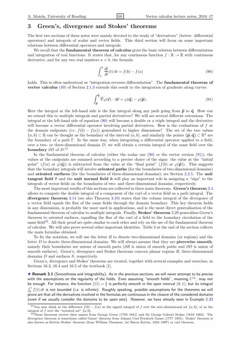
A. Moiola, University of Reading 68 Vector calculus lecture notes, 2016–17
3 Green’s, divergence and Stokes’ theorems
The first two sections of these notes were mainly devoted to the study of “derivatives” (better: differentialoperators) and integrals of scalar and vector fields. This third section will focus on some importantrelations between differential operators and integrals.
We recall that the fundamental theorem of calculus gives the basic relation between differentiationand integration of real functions. It states that, for any continuous function f : R → R with continuousderivative, and for any two real numbers a < b, the formula
∫ b
a
df
dt(t) dt = f(b)− f(a) (90)
holds. This is often understood as “integration reverses differentiation”. The fundamental theorem ofvector calculus (49) of Section 2.1.3 extends this result to the integration of gradients along curves:
∫ ~q
~p
~∇ϕ(~r) · d~r = ϕ(~q)− ϕ(~p). (91)
Here the integral at the left-hand side is the line integral along any path going from ~p to ~q. How canwe extend this to multiple integrals and partial derivatives? We will see several different extensions. Theintegral at the left-hand side of equation (90) will become a double or a triple integral and the derivativewill become a vector differential operator involving partial derivatives. How is the evaluations of f atthe domain endpoints (i.e. f(b) − f(a)) generalised to higher dimensions? The set of the two valuesa, b ⊂ R can be thought as the boundary of the interval (a, b), and similarly the points ~p, ~q ⊂ R3 arethe boundary of a path Γ. In the same way, when integrating a differential operator applied to a field,over a two- or three-dimensional domain D, we will obtain a certain integral of the same field over theboundary ∂D of D.31
In the fundamental theorem of calculus (either the scalar one (90) or the vector version (91)), thevalues at the endpoints are summed according to a precise choice of the signs: the value at the “initialpoint” (f(a) or ϕ(~q)) is subtracted from the value at the “final point” (f(b) or ϕ(~p)). This suggeststhat the boundary integrals will involve oriented paths (for the boundaries of two-dimensional domains)and oriented surfaces (for the boundaries of three-dimensional domains); see Section 2.2.5. The unittangent field τ and the unit normal field n will play an important role in assigning a “sign” to theintegrals of vector fields on the boundaries of two- and three-dimensional domains, respectively.
The most important results of this sections are collected in three main theorems. Green’s theorem 3.4allows to compute the double integral of a component of the curl of a vector field as a path integral. Thedivergence theorem 3.14 (see also Theorem 3.10) states that the volume integral of the divergence ofa vector field equals the flux of the same fields through the domain boundary. This key theorem holdsin any dimensions, is probably the most used in applications, and is the most direct generalisation of thefundamental theorem of calculus to multiple integrals. Finally, Stokes’ theorem 3.28 generalises Green’stheorem to oriented surfaces, equalling the flux of the curl of a field to the boundary circulation of thesame field32. All their proof are quite similar to each other and rely on the use of the fundamental theoremof calculus. We will also prove several other important identities. Table 3 at the end of the section collectsthe main formulas obtained.
To fix the notation, we will use the letter R to denote two-dimensional domains (or regions) and theletter D to denote three-dimensional domains. We will always assume that they are piecewise smooth,namely their boundaries are unions of smooth parts (∂R is union of smooth paths and ∂D is union ofsmooth surfaces). Green’s, divergence and Stokes theorems concern planar regions R, three-dimensionaldomains D and surfaces S, respectively.
Green’s, divergence and Stokes’ theorems are treated, together with several examples and exercises, inSections 16.3, 16.4 and 16.5 of the textbook [1].
⋆ Remark 3.1 (Smoothness and integrability). As in the previous sections, we will never attempt to be precisewith the assumptions on the regularity of the fields. Even assuming “smooth fields”, meaning C∞, may notbe enough. For instance, the function f(t) = 1
t is perfectly smooth in the open interval (0, 1), but its integral∫ 1
0f(t) dt is not bounded (i.e. is infinite). Roughly speaking, possible assumptions for the theorems we will
prove are that all the derivatives involved in the formulas are continuous in the closure of the considered domains(even if we usually consider the domains to be open sets). However, we have already seen in Example 2.33
31You may think at the difference f(b) − f(a) as the signed integral of f over the zero-dimensional set a, b, or as theintegral of f over the “oriented set” a, b.
32These theorems receive their names from George Green (1793–1841) and Sir George Gabriel Stokes (1819–1903). Thedivergence theorem is sometimes called Gauss’ theorem from Johann Carl Friedrich Gauss (1777–1855). Stokes’ theorem isalso known as Kelvin–Stokes’ theorem (from William Thomson, 1st Baron Kelvin, 1824–1907) or curl theorem.
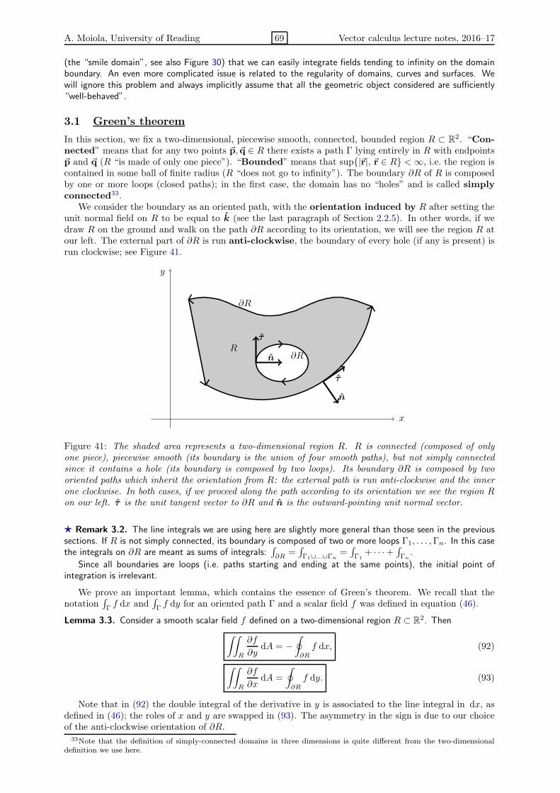
A. Moiola, University of Reading 69 Vector calculus lecture notes, 2016–17
(the “smile domain”, see also Figure 30) that we can easily integrate fields tending to infinity on the domainboundary. An even more complicated issue is related to the regularity of domains, curves and surfaces. Wewill ignore this problem and always implicitly assume that all the geometric object considered are sufficiently“well-behaved”.
3.1 Green’s theorem
In this section, we fix a two-dimensional, piecewise smooth, connected, bounded region R ⊂ R2. “Con-nected” means that for any two points ~p, ~q ∈ R there exists a path Γ lying entirely in R with endpoints~p and ~q (R “is made of only one piece”). “Bounded” means that sup|~r|, ~r ∈ R <∞, i.e. the region iscontained in some ball of finite radius (R “does not go to infinity”). The boundary ∂R of R is composedby one or more loops (closed paths); in the first case, the domain has no “holes” and is called simplyconnected33.
We consider the boundary as an oriented path, with the orientation induced by R after setting theunit normal field on R to be equal to k (see the last paragraph of Section 2.2.5). In other words, if wedraw R on the ground and walk on the path ∂R according to its orientation, we will see the region R atour left. The external part of ∂R is run anti-clockwise, the boundary of every hole (if any is present) isrun clockwise; see Figure 41.
x
y
R
∂R
∂R
τ
n
τ
n
Figure 41: The shaded area represents a two-dimensional region R. R is connected (composed of onlyone piece), piecewise smooth (its boundary is the union of four smooth paths), but not simply connectedsince it contains a hole (its boundary is composed by two loops). Its boundary ∂R is composed by twooriented paths which inherit the orientation from R: the external path is run anti-clockwise and the innerone clockwise. In both cases, if we proceed along the path according to its orientation we see the region Ron our left. τ is the unit tangent vector to ∂R and n is the outward-pointing unit normal vector.
⋆ Remark 3.2. The line integrals we are using here are slightly more general than those seen in the previoussections. If R is not simply connected, its boundary is composed of two or more loops Γ1, . . . ,Γn. In this casethe integrals on ∂R are meant as sums of integrals:
∫∂R
=∫Γ1∪...∪Γn
=∫Γ1
+ · · ·+∫Γn
.
Since all boundaries are loops (i.e. paths starting and ending at the same points), the initial point ofintegration is irrelevant.
We prove an important lemma, which contains the essence of Green’s theorem. We recall that thenotation
∫Γf dx and
∫Γf dy for an oriented path Γ and a scalar field f was defined in equation (46).
Lemma 3.3. Consider a smooth scalar field f defined on a two-dimensional region R ⊂ R2. Then
∫∫
R
∂f
∂ydA = −
∮
∂R
f dx, (92)
∫∫
R
∂f
∂xdA =
∮
∂R
f dy. (93)
Note that in (92) the double integral of the derivative in y is associated to the line integral in dx, asdefined in (46); the roles of x and y are swapped in (93). The asymmetry in the sign is due to our choiceof the anti-clockwise orientation of ∂R.
33Note that the definition of simply-connected domains in three dimensions is quite different from the two-dimensionaldefinition we use here.

A. Moiola, University of Reading 70 Vector calculus lecture notes, 2016–17
Proof of Lemma 3.3. We prove only the first identity (92); the second (93) follows in a similar way. Themain ingredient of the proof is the use of the fundamental theorem of vector calculus in the y-direction toreduce the double integral to a line integral. We split the proof in three main steps.
Part 1. We first consider a y-simple domain R, as in formula (52):
R =xı+ y ∈ R2, s.t. xL < x < xR, a(x) < y < b(x)
,
where xL < xR, a, b : (xL, xR) → R, a(x) < b(x) for all x ∈ (xL, xR). We compute the double integral atthe left-hand side of (92) using the formula for the iterated integral (53) and the fundamental theorem ofcalculus (90) applied to the partial derivative of f in the y-direction:
∫∫
R
∂f
∂ydA
(53)=
∫ xR
xL
∫ b(x)
a(x)
∂f
∂y(x, y) dy dx
(90)=
∫ xR
xL
f(x, y)
∣∣∣∣b(x)
y=a(x)
dx =
∫ xR
xL
(f(x, b(x)
)− f
(x, a(x)
))dx.
(94)
We now consider the boundary integral at the right-hand side of the assertion (92). We split it in fourcomponents, corresponding to the four oriented paths34 in which the boundary ∂R is divided, as in theleft plot of Figure 42:
∮
∂R
f dx =
∫
ΓS
f dx+
∫
ΓE
f dx+
∫
ΓN
f dx+
∫
ΓW
f dx.
We first note that the two lateral paths ΓE = xRı+y, a(xR) ≤ y ≤ b(xR) and ΓW = xLı+y, a(xL) ≤y ≤ b(xL) are vertical. The integrals
∫· · · dx take into account only the horizontal component of the
curve total derivative (see the definition in (46)) which is zero on these two segments, thus the two verticalpaths do not give any contribution to the integral at the right-hand side of (92).35 The x components of theparametrisations of the two remaining curvilinear sides can be chosen as affine functions (ı ·~cS(t) = xL+ tand ı · ~cN (t) = xR − t), while the y components depend on x through the boundary functions a and b(y = b(x) on ΓN and y = a(x) on ΓS), thus we can write the integral
∫· · · dx as in formula (48):
∮
∂R
f dx =
∫
ΓS
f dx+
∫
ΓE
f dx
︸ ︷︷ ︸=0
+
∫
ΓN
f dx+
∫
ΓW
f dx
︸ ︷︷ ︸=0
(48)=
∫ xR
xL
(f(x, a(x)
)− f
(x, b(x)
))dx
(94)= −
∫∫
R
∂f
∂ydA,
which is the assertion (92). We have concluded the proof for y-simple domains.Part 2. We now consider a region R that is the union of two non-overlapping subregions R1 and R2
(i.e. R1 ∪ R2 = R and R1 ∩ R2 = ∅, being quite imprecise with open and closed sets) such that on bothR1 and R2 equation (92) holds true. Then we prove that the same equation holds also on the whole of R.
We denote by Γ = ∂R1 ∩ ∂R2 the intersection of the boundaries of the two subregions. This is a paththat cuts R in two; if the domain R is not simply-connected, i.e. it contains some holes, then the interfaceΓ might be composed of two or more disconnected paths. We fix on Γ the same orientation of ∂R1 andwe note that this is opposite to the orientation of ∂R2; see the right plot of Figure 42. Combining the
34The path ΓW collapses to a point if a(xL) = b(xL) and similarly the path ΓE if a(xR) = b(xR); see e.g. Figure 25.35To verify this in formulas, we can write explicitly the parametrisations of the four sides:
ΓS : ~cS(t) = (xL + t)ı + a(xL + t),d~cS
dt(t) = ı+ a′(xL + t), 0 < t < xR − xL,
ΓE : ~cE(t) = xRı+(a(xR) + t
),
d~cE
dt(t) = , 0 < t < b(xR)− a(xR),
ΓN : ~cN (t) = (xR − t)ı + b(xR − t),d~cN
dt(t) = −ı− b′(xR − t), 0 < t < xR − xL,
ΓW : ~cW (t) = xLı+(b(xL)− t
),
d~cW
dt(t) = −, 0 < t < b(xL)− a(xL).
We see that the two vertical paths ΓE and ΓW do not give any contribution to the integral at the right-hand side of (92):
∫
ΓE
f dx(46)=
∫
ΓE
f ı · d~r (44)=
∫ b(xR)−a(xR)
0f(~cE(t)
)ı · d~cE
dt(t) dt =
∫ b(xR)−a(xR)
0f(~cE(t)
)ı · ︸︷︷︸=0
dt = 0;
and similarly on ΓW .
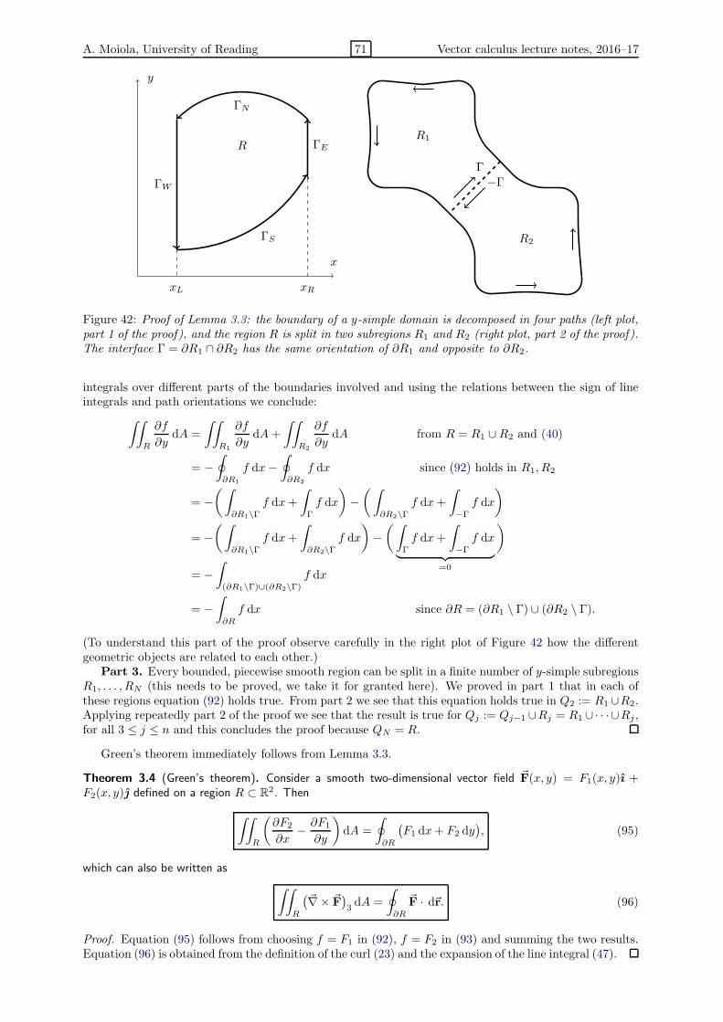
A. Moiola, University of Reading 71 Vector calculus lecture notes, 2016–17
x
y
ΓS
ΓN
ΓE
ΓW
R
xL xR
R1
R2
Γ−Γ
Figure 42: Proof of Lemma 3.3: the boundary of a y-simple domain is decomposed in four paths (left plot,part 1 of the proof), and the region R is split in two subregions R1 and R2 (right plot, part 2 of the proof).The interface Γ = ∂R1 ∩ ∂R2 has the same orientation of ∂R1 and opposite to ∂R2.
integrals over different parts of the boundaries involved and using the relations between the sign of lineintegrals and path orientations we conclude:
∫∫
R
∂f
∂ydA =
∫∫
R1
∂f
∂ydA+
∫∫
R2
∂f
∂ydA from R = R1 ∪R2 and (40)
= −∮
∂R1
f dx−∮
∂R2
f dx since (92) holds in R1, R2
= −(∫
∂R1\Γf dx+
∫
Γ
f dx
)−(∫
∂R2\Γf dx+
∫
−Γ
f dx
)
= −(∫
∂R1\Γf dx+
∫
∂R2\Γf dx
)−(∫
Γ
f dx+
∫
−Γ
f dx
︸ ︷︷ ︸=0
)
= −∫
(∂R1\Γ)∪(∂R2\Γ)f dx
= −∫
∂R
f dx since ∂R = (∂R1 \ Γ) ∪ (∂R2 \ Γ).
(To understand this part of the proof observe carefully in the right plot of Figure 42 how the differentgeometric objects are related to each other.)
Part 3. Every bounded, piecewise smooth region can be split in a finite number of y-simple subregionsR1, . . . , RN (this needs to be proved, we take it for granted here). We proved in part 1 that in each ofthese regions equation (92) holds true. From part 2 we see that this equation holds true in Q2 := R1∪R2.Applying repeatedly part 2 of the proof we see that the result is true for Qj := Qj−1 ∪Rj = R1 ∪· · · ∪Rj ,for all 3 ≤ j ≤ n and this concludes the proof because QN = R.
Green’s theorem immediately follows from Lemma 3.3.
Theorem 3.4 (Green’s theorem). Consider a smooth two-dimensional vector field ~F(x, y) = F1(x, y)ı +F2(x, y) defined on a region R ⊂ R2. Then
∫∫
R
(∂F2
∂x− ∂F1
∂y
)dA =
∮
∂R
(F1 dx+ F2 dy
), (95)
which can also be written as
∫∫
R
(~∇× ~F
)3dA =
∮
∂R
~F · d~r. (96)
Proof. Equation (95) follows from choosing f = F1 in (92), f = F2 in (93) and summing the two results.Equation (96) is obtained from the definition of the curl (23) and the expansion of the line integral (47).

A. Moiola, University of Reading 72 Vector calculus lecture notes, 2016–17
Remark 3.5 (Green’s theorem for three-dimensional fields in two-dimensional domains). We have stated Green’s
theorem for a two-dimensional vector field ~F(x, y) = F1ı+ F2. If ~F is any three-dimensional, smooth vector
field, i.e. ~F(x, y, z) = F1 ı + F2 + F3k may depend also on the z coordinate and have three non-zerocomponents, formula (96) still holds true. In this case, we think at R ⊂ R2 as lying in the xy-plane of R3 (theplane z = 0). Indeed, the left-hand side of the equation is not affected by this modification as (from the
definition of the curl (23)) the third component of the curl (~∇ × ~F)3 = ∂F2
∂x − ∂F1
∂y does not involve neither
F3 nor the partial derivative in z. Similarly, the right-hand side of (96) is not modified because the circulation
of ~F along ∂R is the integral of the scalar product of ~F and the total derivative of the curve defining ∂R (see(44)), whose z-component vanish, thus the component F3 does not contribute to the line integral.
Example 3.6. Use Green’s theorem to compute the circulation of ~F = (2xy + y2)ı+ x2 along the boundaryof the bounded domain R delimited by the line y = x and the parabola y = x2.
The domain R can be written as R = ~r ∈ R2, 0 < x < 1, x2 < y < x; see the left plot in Figure 43.
The curl of the given field is ~∇× ~F = (2x− 2x− 2y)k = −2yk. Then, Green’s theorem gives
∮
∂R
~F · d~r (96)=
∫∫
R
(~∇× ~F)3 dA(53)=
∫ 1
0
(∫ x
x2
(−2y) dy
)dx =
∫ 1
0
(−x2 + x4) dy =1
5− 1
3= − 2
15.
Of course, it is possible to directly compute the circulation, but the calculation is a bit longer, as we haveto split the boundary in the straight segment ΓS (e.g. parametrised by ~a(t) = (1 − t)(ı + ), 0 < t < 1)
and the parabolic arc ΓP (e.g. parametrised by ~b(t) = tı + t2, 0 < t < 1). (Recall the parametrisations ofRemark 1.24 and that the boundary must be oriented anti-clockwise.) Then we have
∮
∂R
~F · d~r =∫
ΓS
~F · d~r+∫
ΓP
~F · d~r
=
∫ 1
0
(3(1− t)2 ı+ (1− t)2
)· (−ı− ) dt+
∫ 1
0
((2t3 + t4)ı+ t2
)· (ı+ 2t) dt
= −4
∫ 1
0
(1 − t)2 dt+
∫ 1
0
(4t3 + t4) dt = −4
3+ 1 +
1
5= − 2
15.
x
y
ı
R
x
y
ı 2ı−2ı
R
Figure 43: Left plot: the domain R = ~r ∈ R2, 0 < x < 1, x2 < y < x in Example 3.6.Right plot: the half ellipse R = xı+ y ∈ R2, 1
4x2 + y2 < 1, y > 0 in Exercise 3.8.
Exercise 3.7. Demonstrate Green’s theorem for the vector field ~F = (x + 2y)(ı + 3) and the discxı+ y, such that x2 + y2 < 4.Exercise 3.8. Demonstrate Green’s theorem for ~F = y2ı on the half-ellipse R = xı+y ∈ R2, 1
4x2+y2 <
1, y > 0 (right plot in Figure 43).
Example 3.9 (Measuring areas with line integrals). A (perhaps) surprising application of Green’s theorem isthe possibility of measuring the area of a planar region R by computing only line integrals on its boundary36.To do this, we need a vector field ~F such that the integrand on R in (95) is everywhere equal to one, namely∂F2
∂x − ∂F1
∂y = 1. Several choices are possible, for instance ~F = −yı, ~F = x, or ~F = 12 (−yı + x). Each of
these gives rise to a line integral that computes the area of R:
Area(R) =
∫∫
R
dA = −∮
∂R
y dx =
∮
∂R
xdy =1
2
∮
∂R
(−y dx+ dy).
36The possibility of computing areas with line integrals should not be a surprise: we already know that the area of ay-simple domain (52), for example, can be computed as
Area(R) =
∫∫
R
dA =
∫ xR
xL
(∫ b(x)
a(x)dy
)dx =
∫ xR
xL
(b(x)− a(x)
)dx
which is nothing else than −∮∂R
y dx. This is also the formula for the area of the region comprised between two graphs youalready know from first year.

A. Moiola, University of Reading 73 Vector calculus lecture notes, 2016–17
In Section 2.1.2, we defined the unit tangent vector field τ = d~adt /∣∣d~adt
∣∣ of an oriented path Γ defined bythe curve ~a. If Γ = ∂R is the boundary of R (with the orientation convention described above), then theoutward pointing unit normal vector n on ∂R is related to the unit tangent τ by the formulas
n = τ × k = t2ı− t1, τ = k × n = −n2ı+ n1, (n1 = t2, n2 = −t1); (97)
see Figure 41. (Note that, if R contains a hole, then on the the corresponding part of the boundary the
vector field n points out of R and into the hole.) For a vector field ~F = F1 ı + F2, choosing f = F1 in(93), f = F2 in (92), and summing the resulting equations we obtain
∫∫
R
(∂F1
∂x+∂F2
∂y
)dA
(92),(93)=
∮
∂R
(F1 dy − F2 dx
)
(46)=
∮
∂R
(F1− F2 ı
)· d~r
(2)=
∮
∂R
(k × ~F
)· d~r
(45)=
∮
∂R
((k × ~F) · τ
)ds
Ex. 1.15=
∮
∂R
((τ × k) · ~F
)ds
(97)=
∮
∂R
(~F · n
)ds.
This is the proof of the divergence theorem in two dimensions.
Theorem 3.10 (Divergence theorem in two-dimensions). Let ~F = F1 ı+F2 be a smooth vector field definedin a region R ⊂ R2 with outward pointing unit normal vector field n. Then
∫∫
R
(∂F1
∂x+∂F2
∂y
)dA =
∮
∂R
~F · n ds. (98)
The integrand in the double integral at the left-hand side of (98) is the two-dimensional divergence~∇ · ~F of ~F.
Example 3.11. As in Example 3.6, consider the vector field ~F = (2xy + y2)ı+ x2 and the bounded domain
R delimited by the line y = x and the parabola y = x2. Compute the “flux”37∮∂R
~F · ~n ds of ~F through ∂R.We simply apply the divergence theorem (98):
∮
∂R
~F · ~n ds =
∫∫
R
(∂F1
∂x+∂F2
∂y
)dA =
∫∫
R
2y dA =
∫ 1
0
(∫ x
x2
2y dy
)dx =
2
15,
with the same computation as in the previous example. The direct computation of the contour integral is slightlymore complicated in this case than in Example 3.6, in that it requires the calculation of the outward-pointingunit normal vector field.
Exercise 3.12. Prove the second formula in (97) without using the expansion of the vectors in components.You can find a helpful formula in the exercises in Section 1.1.
3.2 The divergence theorem
In this section we consider a three-dimensional domain D ⊂ R3 and we assume it to be piecewise smooth,bounded and connected. As in the previous section, we start with a preliminary lemma.
Lemma 3.13. Let f be a smooth scalar field on D. Then we have
∫∫∫
D
∂f
∂zdV =
∫∫
∂D
f k · d~S. (99)
Here the surface ∂D is equipped with outward-pointing unit normal vector field n.
37Note that here the word “flux” is used to denote the contour integral of the normal component of a two-dimensionalfield, as opposed to the surface integral of the normal component in three dimensions.

A. Moiola, University of Reading 74 Vector calculus lecture notes, 2016–17
Proof. The proof is very similar to that of Lemma 3.3 (in a sense, it is its extension to three dimensions).As in that case, we divide the proof in three parts: the first is devoted to simple domains, the secondextends the result to the unions of two such simple domains, the third completes the extension to generaldomains by partitioning these in simpler parts. Once more, the basic instrument in the proof is thefundamental theorem of calculus.
Part 1. We consider a z-simple domain as that introduced at the beginning of Section 2.2.3:
D =xı+ y+ zk s. t. xL < x < xR, a(x) < y < b(x), α(x, y) < z < β(x, y)
,
where xL < xR are two real numbers, a, b : [xL, xR] → R two real functions (with a < b), and α, β : R → R
two scalar fields in two variables (with α < β). We call R the planar region R = xı + y s. t. xL < x <xR, a(x) < y < b(x), the projection of D on the xy-plane. See a representation of D and R in Figure 44.
The boundary ∂D is composed of six (curvilinear) faces38. Four of these faces are vertical, as they liestraight above the four (curvilinear) sides of R. Thus on these faces the outward-pointing unit normal
vector field n has zero vertical component k · n, and the corresponding terms∫∫
f k · d~S in the surfaceintegral at the right-hand side of (99) vanish.39
On the other hand, the top face ST is the graph of the two-dimensional field β : R → R. Thecontribution to the surface integral at the right-hand side of (99) given by ST is the flux of the vector fieldf k (whose first two components are constantly zero) through ST itself, and can be reduced to a doubleintegral on R using formula (74):
∫∫
ST
f(x, y, z) k · d~S =
∫∫
R
f(x, y, β(x, y)
)dA.
Similarly, the bottom face SB is the graph of the two-dimensional field α : R → R. However, on this face,the outward-pointing unit normal vector field n points downward, opposite to the convention stipulatedin Section 2.2.5 for graph surfaces. Thus the sign in (74) needs to be reversed and the contribution of SB
to the right-hand side of (99) reads
∫∫
ST
f(x, y, z) k · d~S = −∫∫
R
f(x, y, α(x, y)
)dA.
To conclude the proof of the first part we expand the right-hand side of the identity in the assertion in asum over the faces of D and use the fundamental theorem of calculus to transform it into a triple integral:
∫∫
∂D
f k · d~S =
∫∫
ST
f k · d~S+
∫∫
SB
f k · d~S
+
∫∫
SW
f k · d~S+
∫∫
SS
f k · d~S+
∫∫
SE
f k · d~S+
∫∫
SN
f k · d~S︸ ︷︷ ︸
=0 (k·n=0)
=
∫∫
R
f(x, y, β(x, y)
)dA−
∫∫
R
f(x, y, α(x, y)
)dA
=
∫∫
R
(f(x, y, β(x, y)
)− f
(x, y, α(x, y)
))dA
(90)=
∫∫
R
(∫ β(x,y)
α(x,y)
∂f
∂z(x, y, z) dz
)dA (fundamental theorem of calculus)
(62)=
∫∫∫
D
∂f
∂z(x, y, z) dV (triple integral as an iterated integral).
38Actually, if a(xL) = b(xL) or a(xR) = b(xR), then the left and right faces are collapsed to a segment and the totalnumber of faces is reduced to 5 or 4. The number of non-empty faces can be even lower, consider the following example:−1 < x < 1,−
√x2 + y2 < y <
√x2 + y2,
√1− x2 − y2 < z < 2
√1− x2 − y2. How many non-empty faces does this
z-simple domain have?39More explicitly, the faces and the corresponding unit normals can be written as:
n(~r) =
nW = −ı onx = xL, a(xL) < y < b(xL), α(xL, y) < z < β(xL, y)
,
nS = a′(x)ı−√1+(a′(x))2
onxL < x < xR, y = a(x), α
(x, a(x)
)< z < β
(x, a(x)
),
nE = ı onx = xR, a(xR) < y < b(xR), α(xR, y) < z < β(xR, y)
,
nN =−b′(x)ı+√1+(b′(x))2
onxL < x < xR, y = b(x), α
(x, b(x)
)< z < β
(x, b(x)
).
You can verify these expressions for n by finding two tangent vectors and checking that they are orthogonal to n.

A. Moiola, University of Reading 75 Vector calculus lecture notes, 2016–17
y
z
x
xL
xR
a(x) b(x)R
DnN
SN
nT
ST = β(R)
nE
SE
NSW
E
Figure 44: A representation of the the z-simple domain in the first part of the proof of Lemma 3.13. Thebottom face SB is that underneath, the west face SW is behind D and the south face SS is on the left ofthe figure. The outward-pointing unit vector field n on SW , SS, SE and SN , has zero vertical componentn · k. The fundamental theorem of calculus is applied along all vertical segments connecting the bottomface with the top face.
Part 2. We now show the following: if a domain D is disjoint union of two subdomains D1 and D2,and if identity (99) holds in both of them, then the same identity holds in D.
We denote by Σ = ∂D1 ∩ ∂D2 the interface between the subdomains and with n1, n2 the outward-pointing unit normal vector fields on ∂D1 and ∂D2, respectively. Then ∂D1 = Σ ∪ (∂D1 ∩ ∂D) (and∂D2 = Σ ∪ (∂D2 ∩ ∂D)), n1 = −n2 on Σ and n1 = n on ∂D1 ∩ ∂D (similarly n2 = n on ∂D2 ∩ ∂D).Combining everything we have the assertion:
∫∫∫
D
∂f
∂zdV =
∫∫∫
D1
∂f
∂zdV +
∫∫∫
D2
∂f
∂zdV
=
∫∫
∂D1
f k · n1 dS +
∫∫
∂D2
f k · n2 dS
=
∫∫
∂D1∩∂D
f k · n1 dS +
∫∫
Σ
f k · n1 dS +
∫∫
∂D2∩∂D
f k · n2 dS +
∫∫
Σ
f k · n2 dS
=
∫∫
(∂D1∩∂D)∪(∂D2∩∂D)
f k · n dS +
∫∫
Σ
(f k · n1 + f k · n2︸ ︷︷ ︸=0
) dS
=
∫∫
∂D
f k d~S.
Part 3. Any “regular” domain can be decomposed in a finite union of disjoint z-simple domains (ofcourse, this should be proved rigorously, here we only assume it since we have not even described in detailthe regularity of the domains). Thus, to conclude the proof of the lemma, we can proceed by induction,exactly as we did in part 3 of Lemma 3.3.
Proceeding as in Lemma 3.13, we can prove that
∫∫∫
D
∂f
∂xdV =
∫∫
∂D
f ı · d~S,∫∫∫
D
∂f
∂ydV =
∫∫
∂D
f · d~S. (100)
From identities (99) and (100) we obtain the following fundamental theorem.
Theorem 3.14 (Divergence theorem in three-dimensions). Let ~F be a smooth vector field defined on D. Then
∫∫∫
D
~∇ · ~F dV =
∫∫
∂D
~F · d~S. (101)
In words: the triple integral over D of the divergence of ~F equals the flux of ~F through the boundary of D.

A. Moiola, University of Reading 76 Vector calculus lecture notes, 2016–17
Proof. We simply sum (99) and (100) applied to the three components of ~F:
∫∫∫
D
~∇ · ~F dV =
∫∫∫
D
(∂F1
∂x+∂F2
∂y+∂F3
∂z
)dV
=
∫∫∫
D
∂F1
∂xdV +
∫∫∫
D
∂F2
∂ydV +
∫∫∫
D
∂F3
∂zdV
=
∫∫
∂D
F1 ı · d~S+
∫∫
∂D
F2 · d~S+
∫∫
∂D
F3k · d~S
=
∫∫
∂D
(F1 ı+ F2+ F3k
)· d~S
=
∫∫
∂D
~F · d~S.
The divergence theorem, together with its corollaries, is one of the most fundamental results in analysisand in calculus. It holds in any dimensions, appears in every sort of theoretical and applied setting (PDEs,differential geometry, fluid dynamics, electromagnetism, . . . ), has a deep physical meaning, is the startingpoint for the design of many numerical methods, and its extension to extremely irregular fields anddomains is very challenging (and indeed it is currently an object of research after two centuries from thefirst discovery of the theorem!).
Remark 3.15 (Intuitive physical interpretation of the divergence theorem). If the vector field ~F represents thevelocity of a fluid, its divergence might be interpreted as a measure of the sources and sinks in the fluid. Thusthe divergence theorem may be interpreted as follows: the total net production of a quantity in a domain equalsthe amount of that quantity that exits the domain through its boundary (per unit of time). For this reason,the divergence theorem is used to formulate many “conservation laws” or “continuity equations” describing theevolution and the conservation of certain physical quantities (e.g. mass, energy, charge,. . . ).
Exercise 3.16. Use the divergence theorem to compute the flux of the field ~F = exı+cos2 x+(x+y+z)kthrough the boundary of the box D = (0, 1)× (−1, 1)× (0, 10).
Exercise 3.17. (Difficult!) Use the divergence theorem to compute∫∫
S(x2 + y2) dS, where S = |~r| = R
is the sphere of radius R centred at the origin. Hint: you need to define a suitable vector field.
Exercise 3.18. Consider the cone C = 0 < z < 1, x2 + y2 < z2. Use the divergence theorem to compute∫∫∫C|~r|2 dV .
Exercise 3.19. (i) Use the divergence theorem to compute the flux of the vector field
~F =1
3(x3 + y3 + z3)ı + yz(z+ yk)
through the boundary of the unit ball B = ~r ∈ R3, |~r| < 1. Hint: use spherical coordinates.
(ii) Find L > 0 such that the flux of ~F through the boundary of the cube CL = (0, L)3 = xı+y+zk, 0 <x, y, z < L is equal to the flux of the same field through the boundary of the unit ball B.
Exercise 3.20. [⋆ Very difficult!] Let D ⊂ R3 be a bounded domain. Prove that
∫ ∫
∂D
~r
|~r|3 · d~S =
4π if the origin lies in D,
0 if the origin lies outside D.
In the exercises above we used the divergence theorem for different purposes: to compute a surfaceintegral over a boundary (by finding a vector field whose normal component on the boundary is given, asin 3.17) and to compute a volume integral (by finding a vector field whose divergence is given, as in 3.18).
⋆ Remark 3.21 (The divergence theorem in one dimension is the fundamental theorem of calculus).The divergence theorems 3.10 and 3.14 directly generalise the fundamental theorem of calculus to higherdimensions. Indeed, a bounded, connected (open) domain in R must be an interval I = (a, b), whose boundaryis composed by two points ∂I = a, b with outward-pointing normal vector n(a) = −1 and n(b) = 1 (aone-dimensional vector is simply a scalar). The “zero-dimensional integral” of a function f on ∂I reduces tothe sum of the two values of f in b and a, and the flux to their difference. A “one-dimensional vector field” isa real function and its divergence is its derivative. So we have
∫
I
f ′(x) dx =
∫
I
~∇ · f(x) dx =
∫
∂I
f(x)n(x) dx = f(b)n(b) + f(a)n(a) = f(b)− f(a).

A. Moiola, University of Reading 77 Vector calculus lecture notes, 2016–17
In the next corollary we show several other identities which follow from equations (99) and (100). Onthe boundary ∂D (or more generally on any oriented surface), we call normal derivative the scalarproduct of the gradient of a scalar field f and the unit normal field n of f , and we denote it by
∂f
∂n:= n · ~∇f.
Corollary 3.22. Let f and g be scalar fields and ~F be a vector field, all defined on a domain D. Then∫∫∫
D
~∇f dV =
∫ ∫
∂D
f ndS, (102)
∫∫∫
D
~∇× ~FdV =
∫ ∫
∂D
n× ~F dS, (103)
∫∫∫
D
(f∆g + ~∇g · ~∇f) dV =
∫ ∫
∂D
f∂g
∂ndS (Green’s 1st identity), (104)
∫∫∫
D
(f∆g − g∆f) dV =
∫ ∫
∂D
(f∂g
∂n− g
∂f
∂n
)dS (Green’s 2nd identity). (105)
Note that identities (102) and (103) are vectorial (the values at the two sides of the equal sign are vectors).
Proof. The proof of identity (102) is very easy:
∫∫∫
D
~∇f dV =
∫∫∫
D
(∂f
∂xı+
∂f
∂y+
∂f
∂zk
)dV
(99),(100)=
∫∫
∂D
(f (ı · n)ı+ f( · n)+ f(k · n)k
)dS =
∫∫
∂D
f ndS.
We prove identity (103) for the first component:
∫∫∫
D
(~∇× ~F)1 dV(23)=
∫∫∫
D
(∂F3
∂y− ∂F2
∂z
)dV
(99),(100)=
∫∫
∂D
(F3 · n− F2k · n
)dS
=
∫∫
∂D
(F3n2 − F2n3
)dS
(2)=
∫∫
∂D
(n× ~F)1 dS;
and the same holds for the second and third components.Using the vector identities of Section 1.4, we have
~∇ · (f ~∇g) (29)= ~∇f · ~∇g + f ~∇ · (~∇g) (24)
= ~∇f · ~∇g + f∆g.
Then, Green’s first identity (104) follows immediately from the application of the divergence theorem 3.14
to the field ~F = f ~∇g. Green’s second identity (105) follows from subtracting from (104) the same identitywith f and g interchanged.
Exercise 3.23. Demonstrate identity (102) for the field f = xyz and the unit cube D = (0, 1)3.
Exercise 3.24. Show that if a smooth scalar field f is harmonic in a domain D and its normal derivativevanishes everywhere on the boundary ∂D, then f is constant.
⋆ Remark 3.25. The two Green’s identities (104) and (105) are particularly important in the theory of partialdifferential equations (PDEs). In particular, several second order PDEs involving the Laplacian operator canbe rewritten using (104) in a “variational form” or “weak form”, which involves a volume integral and aboundary one. This is the starting point for the definition of the most common algorithms for the numericalapproximation of the solutions on a computer, in particular for the finite element method (FEM, you might seeit in a future class). Another common numerical scheme, the boundary element method (BEM), arises fromthe second Green identity (105).
Comparison with scalar calculus 3.26 (Integration by parts in more dimensions). In the first calculus classyou learned how to “integrate by parts”:
∫ b
a
f ′(t)g(t) dt+
∫ b
a
f(t)g′(t) dt = f(b)g(b)− f(a)g(a),
for real functions f, g : [a, b] → R. This is a straightforward consequence of the fundamental theorem ofcalculus (90) and the product rule (fg)′ = f ′g + fg′. How does this extend to higher dimensions? The

A. Moiola, University of Reading 78 Vector calculus lecture notes, 2016–17
product rule was extended to partial derivatives in (8) and to differential operators in Proposition 1.55; we sawin Remark 3.21 that the divergence theorem extends the fundamental theorem of calculus. Several formulasarising from different combinations of these ingredients are usually termed “multidimensional integration byparts”, for example
∫∫∫
D
~∇f · ~GdV +
∫∫∫
D
f ~∇ · ~GdV =
∫∫
∂D
f ~G · d~S,∫∫∫
D
(~∇f)g dV +
∫∫∫
D
f ~∇g dV =
∫∫
∂D
fg n dS,
where f , g are scalar fields and ~G is a vector field on D. For exercise, prove these two identities.
⋆ Remark 3.27 (Differential and integral form of physical laws). The main reason of the importance andubiquity of the divergence theorem in physics and engineering is that it constitutes the relation between the twopossible formulation of many physical laws: the “differential form”, expressed by a partial differential equation,and the “integral form”, expressed by an integral equation. The integral form usually better describes the mainphysical concepts and contains the quantities that can be measured experimentally, while the differential formallows an easier mathematical manipulation. The two forms may lead to different numerical algorithms for theapproximation of the solutions of the equation.
For example, we consider Gauss’ law of electrostatics, you might have already encountered elsewhere. Itsintegral form states that the flux of an electric field ~E (which is a vector field) through a closed surface ∂D(in vacuum) is proportional to the total electrical charge in the volume D bounded by that surface:
∫ ∫
∂D
~E · d~S =
∫∫∫
D
ρ
ε0dV,
where ρ is the charge density (whose integral gives the total charge) and ε0 is a constant of proportionality (the
“vacuum permittivity”). Its differential form reads ~∇ · ~E = ρ/ε0. The divergence theorem immediately allowsto deduce the integral form of Gauss law from the differential one; since the former holds for any domain D,also the converse implication can be proved. Gauss’ law is one of the four celebrated Maxwell’s equations, thefundamental laws of electromagnetism: all of them have a differential and an integral form, related to eachother either by the divergence or Stokes’ theorem.
3.3 Stokes’ theorem
Stokes’ theorem extends Green’s theorem to general oriented surfaces. It states that the flux of the curl ofa vector field through an oriented surface equals the circulation along the boundary of the same surface.
Theorem 3.28 (Stokes’ theorem). Let S ⊂ R3 be a piecewise smooth, bounded, oriented surface with unit
normal field n, and let ~F be a smooth vector field defined on S. Then
∫∫
S
(~∇× ~F) · d~S =
∮
∂S
~F · d~r, (106)
where the boundary ∂S is understood as the oriented path with the orientation inherited from (S, n).
Proof. We prove the theorem only for the special class of surfaces describe in Remark 2.44: we assume Sto be the graph of a two-dimensional field g, i.e. S = ~r = xı+ y+ zk ∈ R3 s.t. xı+ y ∈ R, z = g(x, y)where R ⊂ R2 is a planar region as in Section 3.1. The proof of the theorem in its generality requirespasting together two or more simpler surfaces.
The main idea of the proof is to reduce the two integrals in (106) to similar integrals on the flat regionR and its boundary, using the fact that S is the graph of g, so the variables on S are related to each otherby the equation z = g(x, y). Then one applies Green’s theorem on R.
The surface integral (flux) at the left-hand side of the assertion (106) can easily be transformed into adouble integral over the planar region R by using formula (74):
∫∫
S
(~∇× ~F) · d~S (74)=
∫∫
R
(− (~∇× ~F)1
∂g
∂x− (~∇× ~F)2
∂g
∂y+ (~∇× ~F)3
)dA
(23)=
∫∫
R
(−(∂F3
∂y− ∂F2
∂z
)∂g∂x
−(∂F1
∂z− ∂F3
∂x
)∂g∂y
+(∂F2
∂x− ∂F1
∂y
))dA.
(107)
We denote by ~a : [tI , tF ] → ∂S a curve that parametrises ∂S. The surface S is the graph of g, thus thecomponents of ~a are related one another by the relation a3(t) = g(a1(t), a2(t)). From the chain rule (37)we have da3
dt = ∂g∂x
da1
dt + ∂g∂y
da2
dt . Moreover, the planar curve a1(t)ı + a2(t) is a parametrisation of ∂R,
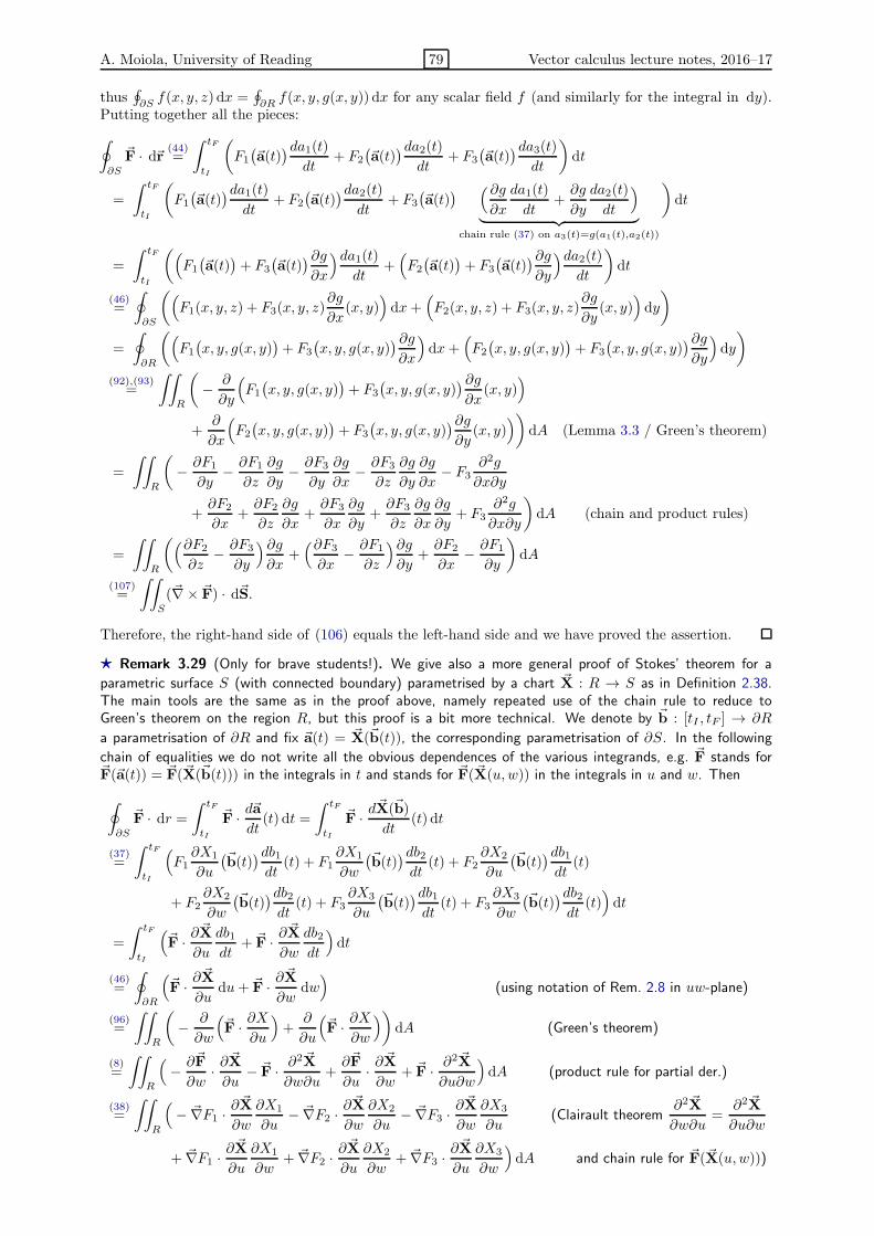
A. Moiola, University of Reading 79 Vector calculus lecture notes, 2016–17
thus∮∂S f(x, y, z) dx =
∮∂R f(x, y, g(x, y)) dx for any scalar field f (and similarly for the integral in dy).
Putting together all the pieces:
∮
∂S
~F · d~r (44)=
∫ tF
tI
(F1
(~a(t)
)da1(t)dt
+ F2
(~a(t)
)da2(t)dt
+ F3
(~a(t)
)da3(t)dt
)dt
=
∫ tF
tI
(F1
(~a(t)
)da1(t)dt
+ F2
(~a(t)
)da2(t)dt
+ F3
(~a(t)
) (∂g∂x
da1(t)
dt+∂g
∂y
da2(t)
dt
)
︸ ︷︷ ︸chain rule (37) on a3(t)=g(a1(t),a2(t))
)dt
=
∫ tF
tI
((F1
(~a(t)
)+ F3
(~a(t)
)∂g∂x
)da1(t)dt
+(F2
(~a(t)
)+ F3
(~a(t)
)∂g∂y
)da2(t)dt
)dt
(46)=
∮
∂S
((F1(x, y, z) + F3(x, y, z)
∂g
∂x(x, y)
)dx+
(F2(x, y, z) + F3(x, y, z)
∂g
∂y(x, y)
)dy
)
=
∮
∂R
((F1
(x, y, g(x, y)
)+ F3
(x, y, g(x, y)
)∂g∂x
)dx+
(F2
(x, y, g(x, y)
)+ F3
(x, y, g(x, y)
)∂g∂y
)dy
)
(92),(93)=
∫∫
R
(− ∂
∂y
(F1
(x, y, g(x, y)
)+ F3
(x, y, g(x, y)
)∂g∂x
(x, y))
+∂
∂x
(F2
(x, y, g(x, y)
)+ F3
(x, y, g(x, y)
)∂g∂y
(x, y)))
dA (Lemma 3.3 / Green’s theorem)
=
∫∫
R
(− ∂F1
∂y− ∂F1
∂z
∂g
∂y− ∂F3
∂y
∂g
∂x− ∂F3
∂z
∂g
∂y
∂g
∂x− F3
∂2g
∂x∂y
+∂F2
∂x+∂F2
∂z
∂g
∂x+∂F3
∂x
∂g
∂y+∂F3
∂z
∂g
∂x
∂g
∂y+ F3
∂2g
∂x∂y
)dA (chain and product rules)
=
∫∫
R
((∂F2
∂z− ∂F3
∂y
)∂g∂x
+(∂F3
∂x− ∂F1
∂z
)∂g∂y
+∂F2
∂x− ∂F1
∂y
)dA
(107)=
∫∫
S
(~∇× ~F) · d~S.
Therefore, the right-hand side of (106) equals the left-hand side and we have proved the assertion.
⋆ Remark 3.29 (Only for brave students!). We give also a more general proof of Stokes’ theorem for a
parametric surface S (with connected boundary) parametrised by a chart ~X : R → S as in Definition 2.38.The main tools are the same as in the proof above, namely repeated use of the chain rule to reduce toGreen’s theorem on the region R, but this proof is a bit more technical. We denote by ~b : [tI , tF ] → ∂R
a parametrisation of ∂R and fix ~a(t) = ~X(~b(t)), the corresponding parametrisation of ∂S. In the following
chain of equalities we do not write all the obvious dependences of the various integrands, e.g. ~F stands for~F(~a(t)) = ~F(~X(~b(t))) in the integrals in t and stands for ~F(~X(u,w)) in the integrals in u and w. Then
∮
∂S
~F · dr =∫ tF
tI
~F · d~adt
(t) dt =
∫ tF
tI
~F · d~X(~b)
dt(t) dt
(37)=
∫ tF
tI
(F1∂X1
∂u
(~b(t)
)db1dt
(t) + F1∂X1
∂w
(~b(t)
)db2dt
(t) + F2∂X2
∂u
(~b(t)
)db1dt
(t)
+ F2∂X2
∂w
(~b(t)
)db2dt
(t) + F3∂X3
∂u
(~b(t)
)db1dt
(t) + F3∂X3
∂w
(~b(t)
)db2dt
(t))dt
=
∫ tF
tI
(~F · ∂
~X
∂u
db1dt
+ ~F · ∂~X
∂w
db2dt
)dt
(46)=
∮
∂R
(~F · ∂
~X
∂udu+ ~F · ∂
~X
∂wdw)
(using notation of Rem. 2.8 in uw-plane)
(96)=
∫∫
R
(− ∂
∂w
(~F · ∂X
∂u
)+
∂
∂u
(~F · ∂X
∂w
))dA (Green’s theorem)
(8)=
∫∫
R
(− ∂~F
∂w· ∂
~X
∂u− ~F · ∂
2 ~X
∂w∂u+∂~F
∂u· ∂
~X
∂w+ ~F · ∂
2 ~X
∂u∂w
)dA (product rule for partial der.)
(38)=
∫∫
R
(− ~∇F1 ·
∂ ~X
∂w
∂X1
∂u− ~∇F2 ·
∂ ~X
∂w
∂X2
∂u− ~∇F3 ·
∂ ~X
∂w
∂X3
∂u(Clairault theorem
∂2 ~X
∂w∂u=
∂2 ~X
∂u∂w
+ ~∇F1 ·∂ ~X
∂u
∂X1
∂w+ ~∇F2 ·
∂ ~X
∂u
∂X2
∂w+ ~∇F3 ·
∂ ~X
∂u
∂X3
∂w
)dA and chain rule for ~F(~X(u,w)))

A. Moiola, University of Reading 80 Vector calculus lecture notes, 2016–17
(16)=
∫∫
R
((J~F− (J~F)T
)∂ ~X∂u
)· ∂
~X
∂wdA (collecting terms, tricky!)
=
∫∫
R
((~∇× ~F)× ∂ ~X
∂u
)· ∂
~X
∂wdA (Remark 1.64)
=
∫∫
R
(~∇× ~F) ·(∂ ~X∂u
× ∂ ~X
∂w
)dA (Exercise 1.15)
(67)=
∫∫
S
(~∇× ~F) · d~S (surface integral formula).
We note an immediate consequence of Stokes’ theorem. If the surface S is the boundary of a three-dimensional domain D, then ∂S is empty (see Remark 2.59). Thus, (106) implies that, for every bounded,
connected, piecewise smooth domain D and for every smooth vector field ~F defined on ∂D, the flux of~∇× ~F on ∂D vanishes: ∫∫
∂D
(~∇× ~F) · d~S = 0.
Note that using the divergence theorem 3.14 and the vector identity ~∇ · (~∇× ~F) = 0 (25) we could have
derived the same identity, but only in the case when ~F was defined (and smooth) in the whole domain D,and not only on its boundary.
Exercise 3.30. Demonstrate Stokes’ theorem for the upper half sphere S = |~r| = 1, z > 0 and the field~F = (2x− y)ı− yz2− y2zk.
Exercise 3.31. Compute∮∂S
|~r|2 dx, with S = z = x2 − y2, 0 < x, y < 1 (cf. Exercise 2.55).
Exercise 3.32. Let f : R3 → R be a scalar field. Prove that the line integral of the product f ~∇f along theboundary of an orientable surface S is zero.
Remark 3.33 (An alternative definition of divergence and curl). The divergence and the curl of a vector field~F are often defined as the following limits (whenever the limits exist):
~∇ · ~F(~r0) = limR→0
1
Vol(BR)
∫ ∫
∂BR
~F · d~S,
a ·(~∇× ~F(~r0)
)= lim
R→0
1
Area(QR(a))
∮
∂QR(a)
~F · d~r,
where BR = ~r ∈ R3, |~r−~r0| < R is the ball of centre ~r0 and radius R, a is a unit vector, and QR(a) is thedisc of centre ~r0, radius R and perpendicular to a. (Note that the curl is defined by its scalar product with
all unit vectors.) Then one proves40 that, if ~F is differentiable, these definitions coincide with those given inSection 1.3. This also provides rigorous, geometric, coordinate-free interpretations of divergence and curl as“spreading” and “rotation” of a vector field, respectively:
The divergence of a vector field ~F is the average of the flux of ~F through an infinitesimal sphere.The curl of ~F is the average of the circulation of ~F around an infinitesimal circle.
Note that also the usual derivative of a real function G : R → R can be defined in a completely analogousway as G′(t) = limR→0
1Length([t−R,t+R])(G(t+R)−G(t−R)). Here, the interpretation is that the derivative
of G is the average of the increment of G in an infinitesimal interval.
⋆ Remark 3.34. With the fundamental theorem of vector calculus we have seen that the line integral from apoint ~p to a point ~q of a gradient is independent of the integration path. In other words,
∫Γ~∇ϕ · d~r depends
only on the scalar field ϕ and the endpoints of Γ, i.e. its boundary ∂Γ (as opposed to the entire path Γ).Stokes’ theorem may be interpreted similarly: the flux of the curl of a vector field through a surface S only
depends on the field itself and the boundary of S (as opposed to the entire surface S). If two surfaces sharethe boundary (e.g. the north and the south hemispheres of the same sphere), the flux of a curl through themwill give the same value. The equivalences of (50) can be translated to this setting:
40If ~∇·~F or ~∇×~F are constant in a neighbourhood of ~r0, these proofs are immediate from divergence and Stokes’ theorem:
limR→0
∫∫∂BR
~F · d~SVol(BR)
(101)= lim
R→0
∫∫∫BR
~∇ · ~FdV
Vol(BR)
(40)= lim
R→0
Vol(BR)~∇ · ~F(~r0)
Vol(BR)= ~∇ · ~F(~r0),
limR→0
∮∂QR(a)
~F · d~rArea(QR(a))
(106)= lim
R→0
∫∫QR(a)
(~∇× ~F) · d~SArea(QR(a))
(40)= lim
R→0
Area(QR(a))(~∇ × ~F(~r0)) · nArea(QR(a))
=(~∇× ~F(~r0)
)· a,
(since n = a on QR(a)); in the general case the proofs require a suitable version of the mean value theorem (attempt towrite the proofs!).

A. Moiola, University of Reading 81 Vector calculus lecture notes, 2016–17
~G = ~∇× ~A
(∃ vector potential for ~G)⇐⇒
∫∫
S
~G · d~Sis independent of S
⇐⇒
∫∫
∂D
~G · d~S = 0
∀ closed surfaces ∂D=⇒
~∇ · ~G = 0
(~G solenoidal)
(where, with “independent of S”, we mean that∫∫
SA
~G · d~S =∫∫
SB
~G · d~S if SA and SB are two surfaces
with ∂SA = ∂SB). The converse of the last implication is true if the domain of ~G does not contain “holes”.
⋆ Remark 3.35. Often the name “Stokes’ theorem” is referred to a much more general version of it, comingfrom the branch of mathematics known as “differential geometry”. This involves the integration of a differentialoperator called “exterior derivative”, simply denoted by “ d”. This acts on “differential forms”, which aregeneralisations of scalar and vector fields defined on a “manifold” Ω, which in turn is an object that generalisesdomains, paths and surfaces to any dimension. This extremely general and deep theorem is stated with a simpleand elegant formula:
∫Ωdω =
∫∂Ωω. The fundamental theorem of (vector) calculus, Green’s, divergence and
Stokes’ theorems are special instances of this result. If you are interested in deepening this topic, take a lookat Chapter 10 of W. Rudin’s book “Principles of mathematical analysis” (this is not an easy read!).
1D (90) Fundamental theoremof calculus
∫ b
a
dφ
dtdt = φ(b)− φ(a)
3D*(49)(91)
Fundamental theoremof vector calculus
∫
Γ
~∇f · d~r = f(~q)− f(~p)
2D (92) Lemma 3.3
∫∫
R
∂f
∂ydA = −
∮
∂R
f dx
2D (93) Lemma 3.3
∫∫
R
∂f
∂xdA =
∮
∂R
f dy
2D (95) Green’s theorem
∫
R
(∂F2
∂x− ∂F1
∂y
)dA =
∮
∂R
(F1 dx+ F2 dy
)
2D (96) Green’s theorem
∫∫
R
(~∇× ~F)3 dA =
∫∫
R
(~∇× ~F) · k dA =
∮
∂R
~F · d~r
2D (98) Divergence theorem
∫∫
R
(~∇ · ~F) dA =
∮
∂R
(F1 dy − F2 dx) =
∮
∂R
~F · n ds
3D(99)(100)
Lemma 3.13
∫∫∫
D
∂f
∂zdV =
∫∫
∂D
f k · d~S
3D (101) Divergence theorem
∫∫∫
D
(~∇ · ~F) dV =
∫∫
∂D
~F · d~S
3D (102) Corollary 3.22
∫∫∫
D
~∇f dV =
∫∫
∂D
f n dS
3D (103) Corollary 3.22
∫∫∫
D
~∇× ~F dV =
∫∫
∂D
~F× n dS
3D (104) Green’s 1st identity
∫∫∫
D
(f∆g + ~∇g · ~∇f) dV =
∫∫
∂D
f∂g
∂ndS
3D (105) Green’s 2nd identity
∫∫∫
D
(f∆g − g∆f) dV =
∫∫
∂D
(f∂g
∂n− g
∂f
∂n
)dS
3D* (106) Stokes’ theorem
∫∫
S
~∇× ~F · d~S =
∫
∂S
~F · d~r
Table 3: A summary of the important integro-differential identities proved in Section 3. Here:Γ is a path with starting point ~p and end point ~q;R ⊂ R2 is a two-dimensional, bounded, connected, piecewise smooth region;D ⊂ R3 is a three-dimensional, bounded, connected, piecewise smooth domain;(S, n) is a piecewise smooth, bounded, oriented surface;φ is a real function;f and g are smooth scalar fields;~F is a smooth vector field.(* Note that the first column of the table denotes the dimension of the space in which the domain ofintegration is defined; the intrinsic dimension of the domain of integration for the fundamental theoremof vector calculus is one (oriented path), and for Stokes’ theorem is two (oriented surface).)

A. Moiola, University of Reading 82 Vector calculus lecture notes, 2016–17
A General overview of the notes
The three main sections of these notes discuss the following general topics:1. differential vector calculus (differentiation of vector quantities);2. integral vector calculus (integration of vector quantities);
3. generalisations of the fundamental theorem of calculus (relation between differentiation and integra-tion of vector quantities).
Section 1.1 recalls some operations involving vectors ~u, ~v, ~w ∈ R3 and scalars λ ∈ R:
inputs outputVector addition: 2 vectors ~u, ~w 7→ vector ~u+ ~wScalar-vector multiplication: a vector ~u and a scalar λ 7→ vector λ~uScalar product: 2 vectors ~u, ~w 7→ scalar ~u · ~wVector product: 2 vectors ~u, ~w 7→ vector ~u× ~wTriple product: 3 vectors ~u, ~v, ~w 7→ scalar ~u · (~v × ~w)
Sections 1.2 introduces different kinds of functions (or fields), taking as input and returning as outputeither scalar values (in R) or vectors (in R3):
Real functions (of real variable) f : R → R t 7→ f(t)Curves ~a : R → R3 t 7→ ~a(t)Scalar fields f : R3 → R ~r 7→ f(~r)
Vector fields ~F : R3 → R3 ~r 7→ ~F(~r)
The fundamental differential operators for scalar and vector fields are the partial derivatives ∂∂x ,
∂∂y and
∂∂z . They can be combined to construct several vector differential operators, as described in Section 1.3.The most important are:
Partial derivatives ∂∂x ,
∂∂y or ∂
∂z scalar 7→ scalar
Gradient ~∇ scalar 7→ vector
Divergence ~∇· (or div) vector 7→ scalar
Curl ~∇× (or curl) vector 7→ vectorLaplacian ∆ scalar 7→ scalar
Proposition 1.52 describes the result of the composition of differential operators.Proposition 1.55 describes the result of the application of differential operators to different products of
scalar and vector fields (generalising the product rule).
Section 1.5 studies some relations between vector fields ~F lying in the kernel (or nullspace) of the
divergence and the curl operators (i.e. solenoidal fields ~∇ · ~F = 0 and irrotational fields ~∇× ~F = ~0) and
those in the image of the gradient and the curl (i.e. fields admitting a scalar potential ~F = ~∇ϕ or a vector
potential ~F = ~∇× ~A).Section 1.6 describes the total derivatives (in t) of curves, denoted d~a
dt .Section 1.7 investigates the differentiation of composition of fields and curves.Sections 2.1 and 2.2 extends the definition of integrals of real functions to:
Type of integral domain of integration integrand notation
Integrals of real functions interval (a, b) real function∫ b
a f dtLine integrals of scalar fields path Γ scalar field
∫Γf ds
Line integrals of vector fields oriented path Γ vector field∫Γ~F · d~r
Double integrals planar domain R ⊂ R2 scalar field∫∫
Rf dA
Triple integrals domain D ⊂ R3 scalar field∫∫∫
D f dVSurface integrals surface S scalar field
∫∫S f dS
Fluxes oriented surface (S, n) vector field∫∫
R~F · d~S
Several theorems establish important relations between integration and differentiation, see Table 3.The most relevant are:
The integral of (the) of a is equal of at/on theon a(n) to the
FTC interval (a, b) derivative function f difference f endpointsFTVC oriented path Γ τ · gradient scalar field f difference f endpoints
Green 2D region R k· curl vector field ~F circulation ~F boundary ∂R
Stokes oriented surface (S, n) n· curl vector field ~F circulation ~F boundary ∂S
Divergence 3D domain D divergence vector field ~F flux ~F boundary ∂D1st domain differential function type of 2nd domainof integration operator or field integral of integration

A. Moiola, University of Reading 83 Vector calculus lecture notes, 2016–17
B Solutions of the exercises
B.1 Exercises of Section 1
Solution of Exercise 1.6. ı · ı = · = k · k = 1, ı · = · ı = ı · k = k · ı = · k = k · = 0.
Solution of Exercise 1.7. Existence. Since ~u|| must be parallel to ~w and ~w 6= ~0, it must have theform ~u|| = α~w for some α ∈ R. Thus ~u⊥ = ~u − ~u|| = ~u − α~w. The orthogonality condition gives0 = ~w · ~u⊥ = ~w · (~u− α~w) = ~w · ~u− α|~w|2, i.e. α = ~w · ~u/|~w|2. Thus the pair
~u|| =~w · ~u|~w|2 ~w, ~u⊥ = ~u− ~u|| = ~u− ~w · ~u
|~w|2 ~w
satisfies all the requests.Uniqueness. Assume by contradiction that two pairs ~u||, ~u⊥ and ~v||, ~v⊥ give an orthogonal decompo-
sition of ~u with respect to ~w. Since ~u|| and ~v|| are both parallel to ~w, they can be written as ~u|| = α~wand ~v|| = β~w. Reasoning as in the existence part of the exercise, we find a unique possible value of α andβ, so ~u|| = ~v|| and consequently ~u⊥ = ~u− ~u|| = ~u− ~v|| = ~v⊥ and there exists only one admissible pair.
Solution of Exercise 1.8. We only need to verify that the two scalar products between ~u× ~w and thetwo vectors are zero:
(~u× ~w) · ~u (2)=((u2w3 − u3w2 )ı+ (u3w1 − u1w3)+ (u1w2 − u2w1)k
)· ~u
= u2w3u1 − u3w2u1 + u3w1u2 − u1w3u2 + u1w2u3 − u2w1u3
= w1(u3u2 − u2u3) + w2(u1u3 − u3u1) + w3(u2u1 − u1u2) = 0,
(~u× ~w) · ~w =((u2w3 − u3w2)ı + (u3w1 − u1w3) + (u1w2 − u2w1)k
)· ~w
= u2w3w1 − u3w2w1 + u3w1w2 − u1w3w2 + u1w2w3 − u2w1w3 = 0.
Solution of Exercise 1.9. We write in detail only ı× and ı× ı, all the other cases are similar:
ı× =
∣∣∣∣∣∣
ı k
1 0 00 1 0
∣∣∣∣∣∣= ı
∣∣∣∣0 01 0
∣∣∣∣−
∣∣∣∣1 00 0
∣∣∣∣+ k
∣∣∣∣1 00 1
∣∣∣∣ = 0ı+ 0+ 1k = k,
ı× ı =
∣∣∣∣∣∣
ı k
1 0 01 0 0
∣∣∣∣∣∣= ı
∣∣∣∣0 00 0
∣∣∣∣−
∣∣∣∣1 01 0
∣∣∣∣+ k
∣∣∣∣1 01 0
∣∣∣∣ = 0ı+ 0+ 0k = ~0.
Solution of Exercise 1.10. The anticommutativity ~w×~u = −~u× ~w follows immediately by computing~w× ~u with Formula (2) and swapping the uj ’s with the wj ’s. From this it follows that ~u× ~u = −~u× ~u,
so 2~u× ~u = ~0.
Solution of Exercise 1.11. We use Exercises 1.9 and 1.10: (ı × ) × = k × = −ı 6= ~0 = ı × ~0 =ı× (× ).
Solution of Exercise 1.12. We prove identity (4) componentwise, namely we verify that the threecomponents on the left-hand side and the right-hand side of the identity agree with each other. Considerthe first component:
[~u× (~v × ~w)
]1
(2)= u2[~v × ~w]3 − u3[~v × ~w]2
(2)= u2(v1w2 − v2w1)− u3(v3w1 − v1w3)
= (u2w2 + u3w3)v1 − (u2v2 + u3v3)w1
= (~u · ~w − u1w1)v1 − (~u · ~v − u1v1)w1
= (~u · ~w)v1 − (~u · ~v)w1
=[(~u · ~w)~v − (~u · ~v)~w
]1.
A similar computation holds for the y- and the z-components, thus the assertion (4) follows.

A. Moiola, University of Reading 84 Vector calculus lecture notes, 2016–17
Solution of Exercise 1.13. Jacobi identity follows from applying three times the identity (4), usingthe commutativity of the scalar product, and cancelling all terms:
~u× (~v × ~w) + ~v × (~w × ~u) + ~w × (~u× ~v)
(4)=(~v(~u · ~w)− ~w(~u · ~v)
)+(~w(~v · ~u)− ~u(~v · ~w)
)+(~u(~w · ~v)− ~v(~w · ~u)
)
= ~u((~w · ~v)− (~v · ~w)
)+(~v(~u · ~w)− (~w · ~u)
)+(~w(~v · ~u)− (~u · ~v)
)= ~0.
To prove Binet–Cauchy identity we expand the left-hand side, collect the positive terms, add and subtractthe term u1w1v1p1 + u2w2v2p2 + u3w3v3p3:
(~u× ~v) · (~w × ~p)
=(
(u2v3 − u3v2)ı+ (u3v1 − u1v3)+ (u1v2 − u2v1)k)
·
(
(w2p3 − w3p2)ı+ (w3p1 − w1p3)+ (w1p2 − w2p1)k)
= u2v3w2p3 + u3v2w3p2 + u3v1w3p1 + u1v3w1p3 + u1v2w1p2 + u2v1w2p1
− u3v2w2p3 − u2v3w3p2 − u1v3w3p1 − u3v1w1p3 − u2v1w1p2 − u1v2w2p1
= u2v3w2p3 + u3v2w3p2 + u3v1w3p1 + u1v3w1p3 + u1v2w1p2 + u2v1w2p1 + (u1w1v1p1 + u2w2v2p2 + u3w3v3p3)
− u3v2w2p3 − u2v3w3p2 − u1v3w3p1 − u3v1w1p3 − u2v1w1p2 − u1v2w2p1 − (u1w1v1p1 + u2w2v2p2 + u3w3v3p3)
= (u1w1 + u2w2 + u3w3)(v1p1 + v2p2 + v3p3)− (u1p1 + u2p2 + u3p3)(w1v1 + w2v2 +w3v3)
= (~u · ~w)(~v · ~p)− (~u · ~p)(~v · ~w).
Lagrange identity is obtained by choosing ~w = ~u and ~p = ~v in the Binet–Cauchy identity and movingthe last term to the left-hand side.
Solution of Exercise 1.15. The formula ~u · (~v × ~w) = ~v · (~w × ~u) = ~w · (~u × ~v) follows immediatelyfrom (5). From this and the anticommutativity of the vector product (Exercise 1.10) we have
~w · (~v × ~u) = −~w · (~u× ~v) = −~u · (~v × ~w), ~u · (~v × ~u) = ~v · (~u× ~u) = 0.
Solution of Exercise 1.18. ⋆ (i) If limj→∞ ~uj = ~u then limj→∞ |~uj − ~u| = 0 by definition. Since0 ≤ |(~uj)1 − u1| ≤ |~uj − ~u| from the definition of vector magnitude, by the sandwich theorem (seeTheorem 4.18 in the Real Analysis lecture notes) we have limj→∞ |(~uj)1 − u1| = 0, which is equivalent tolimj→∞(~uj)1 = u1. Similarly, we can prove limj→∞(~uj)2 = u2 and limj→∞(~uj)3 = u3.
To prove the converse, assume limj→∞(~uj)1 = u1, limj→∞(~uj)2 = u2 and limj→∞(~uj)3 = u3. Then,we obtain the desired convergence simply using the properties of limits and the definition of magnitude:
limj→∞
|~uj − ~u| = limj→∞
√((~uj)1 − u1
)2+((~uj)2 − u2
)2+((~uj)3 − u3
)2
=
√(limj→∞
(~uj)1 − u1)2
+(limj→∞
(~uj)2 − u2)2
+(limj→∞
(~uj)3 − u3)2
= 0.
(ii) It suffices to take a sequence converging to some ~w 6= ~u with |~w| = |~u|. For example, ~uj = ı for
all j ∈ N and ~u = k.
Solution of Exercise 1.19. ⋆ Let D ⊂ R3 be open and denote C := R3 \D its complement. We wantto prove that C is closed. Consider a sequence ~pjj∈N ⊂ C such that limj→∞ ~pj = ~p. To prove that Cis closed we need to prove that ~p ∈ C, which is the same as ~p /∈ D, by definition of set complement. Weproceed by contradiction: if ~p ∈ D was true, then there would exist ǫ > 0 such that all points at distancesmaller than ǫ from ~p were in D. But from limj→∞ |~pj−~p| = 0, there exists a ~pj in the sequence (actually,infinitely many) at distance smaller than ǫ from ~p but belonging to C. So we have a contradiction: ~pmust belong to C, thus C is closed.
Now we prove the second statement (the vice versa), which is very similar. Let C ⊂ R3 be closed anddenote D := R3\C its complement. We want to prove that D is open. Again, we proceed by contradiction:if D were not open, there would be a point ~p ∈ D such that for all ǫ > 0 we have a point ~pǫ /∈ D (i.e.~pǫ ∈ C) such that |~p−~pǫ| < ǫ. We fix a real positive sequence ǫj converging to 0 (e.g. ǫj = 1/j). Then bythe contradiction assumption there exists ~pj ∈ C such that |~pj − ~p| < ǫj → 0. Thus limj→∞ ~pj = ~p. AsC is closed, this means that ~p ∈ C, but we assumed ~p ∈ D, so we have a contradiction and we conclude.

A. Moiola, University of Reading 85 Vector calculus lecture notes, 2016–17
Solution of Exercise 1.29. (We expand p(~r) = |~r|2x2 = x2+y2+z2
x2 = 1 + y2+z2
x2 .)
f(~r) = xyez,∂f
∂x= yez,
∂f
∂y= xez ,
∂f
∂z= xyez = f ;
g(~r) =xy
y + z,
∂g
∂x=
y
y + z,
∂g
∂y=
xz
(y + z)2,
∂g
∂z=
−xy(y + z)2
;
h(~r) = log(1 + z2eyz),∂h
∂x= 0,
∂h
∂y=
z3eyz
1 + z2eyz,
∂h
∂z=
(2z + yz2)eyz
1 + z2eyz;
ℓ(~r) =√x2 + y4 + z6,
∂ℓ
∂x=
x√x2 + y4 + z6
,∂ℓ
∂y=
2y3√x2 + y4 + z6
,∂ℓ
∂z=
3z5√x2 + y4 + z6
;
m(~r) = xy = e(log x)y,∂m
∂x=y
xe(log x)y ∂y
∂y= e(log x)y log x
∂m
∂z= 0;
p(~r) =|~r|2x2
∂m
∂x=
−2y2 − 2z2
x3,
∂y
∂y=
2y
x2,
∂m
∂z=
2z
x2.
Solution of Exercise 1.34.
~∇f = yez ı+ xez + xyezk, ~∇g = y
y + zı+
xz
(y + z)2− xy
(y + z)2k,
~∇h =z3eyz+ (2z + yz2)eyzk
1 + z2eyz, ~∇ℓ = xı+ 2y3+ 3z5k√
x2 + y4 + z6,
~∇m =y
xe(log x)y ı+ e(log x)y log x = y xy−1ı+ xy log x, ~∇p = −2y2 − 2z2
x3ı+
2y+ 2zk
x2.
Solution of Exercise 1.35. The field s is a polynomial in three variables, so its gradient is easy tocompute:
~∇s(~r) = ~∇(|~r|2) = ~∇(x2 + y2 + z2) = 2xı+ 2y+ 2zk = 2~r.
To compute ~∇m we use a simple trick (otherwise we can compute it directly). For α ∈ R, define thereal function Gα(t) := tα/2, whose derivative is Gα
′(t) = (α/2)tα/2−1. Using the chain rule (14) for thegradient we obtain the gradient of |~r|α:
~∇(|~r|α) = ~∇(s(~r)α/2
)= ~∇
(Gα
(s(~r)
))= Gα
′(s(~r))~∇s(~r) = α
2
(s(~r)
)α/2−12~r = α
(|~r|2)α/2−1
~r = α|~r|α−2~r.
The field m(~r) = |~r| corresponds to the case α = 1, so ~∇m(~r) = ~r/|~r|, as required.Solution of Exercise 1.37. The level surfaces of f = (2x + y)3 are the sets ~r, (2x + y)3 = C, orequivalently ~r, 2x+ y = C. These are parallel planes. They are all perpendicular to the xy-plane, so k
is tangent to each one of these planes. They intersect the xy-plane in the lines 2x + y = C, z = 0, soalso the vector ı− 2 is tangent to all planes in all their points.
We have ~G = 2ez ı+ez , so ~G · k = 0 and ~G · (ı− 2) = 2ez − 2ez = 0, thus ~G is perpendicular to the
level sets of ~G in all points.Alternatively one can check that ~∇f = 3(2x+ y)2(2ı+ ) = 3(2x+ y)2e−z ~G, so ~∇f and ~G are parallel
and we conclude by Proposition 1.33(4).
Solution of Exercise 1.39. We compute the gradient of f and the unit vector in the direction of ~F:
~∇f(~r) = (ex + z2)ı − cos y+ 2xzk,~F(~r)
|~F(~r)|=
xı + √x2 + 1
.
The directional derivative is
∂f
∂F(~r) =
~F(~r)
|~F(~r)|· ~∇f(~r) = xı+ √
x2 + 1·((ex + z2)ı − cos y+ 2xzk
)=x(ex + z2)− cos y√
x2 + 1.
Solution of Exercise 1.41. We simply compute all the partial derivatives:
J~F(~r) =
2 0 00 −2 00 0 0
, J ~G(~r) =
0 z yz 0 xy x 0
, J ~H(~r) =
2x 2y 2z0 0 00 − sin y 0
.

A. Moiola, University of Reading 86 Vector calculus lecture notes, 2016–17
Solution of Exercise 1.44. We first compute the gradients and then all the second derivatives (recallthe identity h(~r) = (x2 + y2 + z2)2 = x4 + y4 + z4 + 2x2y2 + 2x2z2 + 2y2z2):
~∇f = 2xı − 2y, ~∇g = yez ı + xez + xyezk,
~∇h = ~∇(x2 + y2 + z2)2 = 2(x2 + y2 + z2)(2xı + 2y+ 2zk) = 4|~r|2~r,
Hf =
2 0 00 −2 00 0 0
, Hg =
0 ez yez
ez 0 xez
yez xez xyez
,
Hh =
12x2 + 4y2 + 4z2 8xy 8xz
8xy 4x2 + 12y2 + 4z2 8yz8xz 8yz 4x2 + 4y2 + 12z2
,
∆f = 0, ∆g = xyez = g, ∆h = 20|~r|2.
The field f is a “harmonic function”, since its Laplacian vanishes everywhere.
Solution of Exercise 1.46. We only have to compute three derivatives for each field and sum them:
~∇ · ~F =∂(2x)
∂x+∂(−2y)
∂y+∂0
∂z= 2− 2 + 0 = 0,
~∇ · ~G = 0 + 0 + 0 = 0,
~∇ · ~H = 2x+ 0 + 0 = 2x.
Solution of Exercise 1.50. For each field we have to evaluate six partial derivatives (the non-diagonal
terms of the Jacobian matrix J~F) and sum them appropriately:
~∇× ~F = ~0,
~∇× ~G = (x− x)ı + (y − y)+ (z − z)k = ~0,
~∇× ~H = (− sin y − 0)ı+ (2z − 0)+ (0 − 2y)k = − sin y ı+ 2z− 2yk.
Solution of Exercise 1.61. We compute the left-hand side and the right-hand side, starting from thecomputation of the terms appearing in them, and we verify that they give the same result:
~F× ~G = x2exy ı− zexy,
left-hand side = ~∇ · (~F× ~G) = ~∇ · (x2exy ı− zexy) = 2xexy + x2yexy − zxexy = (2x+ x2y − zx)exy;
~∇× ~F = 3y2ı+ + 2xk, ~∇× ~G = xexy ı− yexy,
right-hand side = (~∇× ~F) · ~G− ~F · (~∇× ~G)
= (3y2ı+ + 2xk) · (exyk)− (zı+ x2+ y3k) · (xexy ı− yexy )
= 2xexy − zxexy + x2yexy = (2x− zx+ x2y)exy = left-hand side.
Solution of Exercise 1.62. We first compute the divergence and the curl of the position vector:
~∇ · (~r) = ~∇ · (xı + y+ zk) =∂x
∂x+∂y
∂y+∂z
∂z= 3,
~∇× (~r) = ~∇× (xı + y+ zk) =(∂z∂y
− ∂y
∂z
)ı+
(∂x∂z
− ∂z
∂x
)+
(∂y∂x
− ∂x
∂y
)k = ~0.
(This solves the exercise for α = 0.) To compute divergence and curl of the vector field ~F = |~r|α~r wedecompose it as the product between the scalar field |~r|α (for which we have already computed the gradientin Exercise 1.35) and the vector field ~r, so that we can apply the product rules (29) and (31):
~∇ · (|~r|α~r) (29)= (~∇ ·~r)|~r|α +~r · ~∇(|~r|α)= 3|~r|α +~r ·
(α|~r|α−2~r
)from solution to Exercise 1.35

A. Moiola, University of Reading 87 Vector calculus lecture notes, 2016–17
= (3 + α)|~r|α from ~r ·~r = |~r|2,~∇× (|~r|α~r) (31)
= ~∇(|~r|α)×~r+ |~r|α ~∇×~r︸ ︷︷ ︸=~0
= α|~r|α−2~r×~r︸ ︷︷ ︸=~0
+~0 = ~0.
Solution of Exercise 1.63. (i) Using that for all vectors ~u× ~u = ~0, we have:
~∇× (f ~∇f) (31)= (~∇f)× (~∇f) + f ~∇× (~∇f) (26)
= ~0.(ii) Using vector identities, the chain rule (14) (with G(u) = uℓ) and again ~u× ~u = ~0 for all ~u ∈ R3:
~∇×(fn~∇(f ℓ)
) (31)= ~∇(fn)× ~∇(f ℓ) + fn ~∇×
(~∇
︸ ︷︷ ︸=~0,(26)
(f ℓ))
(14)= (nfn−1~∇f)× (ℓf ℓ−1~∇f) = nℓfn+ℓ−2~∇f × ~∇f = ~0.
Solution of Exercise 1.67. Proceeding as in the example, we obtain the potentials
ϕA = x2 + y3 + ez, ϕC =x4y4
4+z3
3, ~AD =
(xy +
y2
2
)k.
Solution of Exercise 1.68. By direct computation we obtain ~∇~r = ∂x∂x + ∂y
∂y + ∂z∂z = 3, so the position
vector is not solenoidal. Since the jth component of ~r depends only on the jth component of its argu-ment (which is itself!), by definition its curl vanishes, so the position vector field is irrotational. From
equation (15) we have ~∇(|~r|2) = 2~r, so a scalar potential of ~r is 12 |~r|2.
Solution of Exercise 1.69. Simply take ~H = ~F× ~G: by (30) we have~∇·~H = ~∇·(~F× ~G) = (~∇×~F) · ~G− ~F · (~∇×~G) = ~0 · ~G− ~F · ~0 = 0, so ~H is solenoidal.
Solution of Exercise 1.73. If the field ~F is conservative then its scalar potential ϕ satisfies ~F = ~∇ϕ,so by identity (24) we have ~∇ · ~F = ~∇ · (~∇ϕ) = ∆ϕ.
Solution of Exercise 1.74. If the gradient of a scalar field f admits a vector potential ~A, we have that~∇f = ~∇× ~A. If the vector potential itself is conservative, it means that ~A = ~∇ψ for some scalar field ψ.Thus ~∇f = ~∇× ~A = ~∇× ~∇ψ = ~0 by the identity (26). A scalar field whose gradient vanishes everywhereis constant, so the fields sought are simply the constant ones f(~r) = λ for all ~r.
Solution of Exercise 1.75. Using that the curl of a gradient vanishes, we immediately see that theproduct is solenoidal:
~∇ · (~F× ~G)(30)= (~∇× ~F) · ~G− ~F · (~∇× ~G) = (~∇× ~∇ϕ︸ ︷︷ ︸
=~0, (26)
) · ~G− ~F · (~∇× ~∇ψ︸ ︷︷ ︸=~0, (26)
) = 0.
Two easy choices of the potential are possible:
~A := ϕ~∇ψ ⇒ ~∇× ~A(31)= (~∇ϕ)× (~∇ψ) + ϕ ~∇× (~∇ψ)︸ ︷︷ ︸
=0, (26)
= ~F× ~G;
~B := −ψ~∇ϕ ⇒ ~∇× ~B(31)= −(~∇ψ)× (~∇ϕ)− ψ ~∇× (~∇ϕ)︸ ︷︷ ︸
=0, (26)
= −~G× ~F(3)= ~F× ~G.
Solution of Exercise 1.78. We have d~adt (t) = − sin t ı+ cos t and d~b
dt (t) = −2 sin2τ ı+ 2 cos 2τ .
The path of d~adt is again the unit circle, but the initial point is placed in (as opposed to ı as for ~a).
The path of d~bdt is the circle centred at the origin with radius 2. Since ~b moves more quickly than ~a (it
covers the unit circle in “time” π as opposed to 2π) the total derivative, representing its velocity, hasgreater magnitude.
To find a curve whose derivative equals that of ~a it suffices to add a constant vector, e.g. ~c(t) =(3 + cos t)ı+ sin t .

A. Moiola, University of Reading 88 Vector calculus lecture notes, 2016–17
Solution of Exercise 1.79. We simply compute all the terms:
d~a
dt= − sin t ı+ cos t ,
d~b
dt= −2 sin2t ı+ 2 cos 2t ,
(~a · ~b) (1)= cos t cos 2t+ sin t sin 2t,
LHS of (36)ii (~a · ~b)′ = − sin t cos 2t− 2 cos t sin 2t+ cos t sin 2t+ 2 sin t cos 2t
= sin t cos 2t− cos t sin 2t,
RHS of (36)iid~a
dt· ~b+ ~a · d
~b
dt= (− sin t ı+ cos t ) · (cos 2t ı+ sin 2t )
+ (cos t ı+ sin t ) · (−2 sin 2t ı+ 2 cos 2t )
(1)= sin t cos 2t− cos t sin 2t,
(~a× ~b)(2)= (cos t sin 2t− sin t cos 2t)k,
LHS of (36)iiid(~a× ~b)
dt= (− sin t sin 2t+ 2 cos t cos 2t− cos t cos 2t+ 2 sin t sin 2t)k
= (cos t cos 2t+ sin t sin 2t)k = cos(2t− t)k = cos t k,
RHS of (36)iiid~a
dt× ~b+ ~a× d~b
dt= (− sin t ı+ cos t )× (cos 2t ı+ sin 2t )
+ (cos t ı+ sin t )× (−2 sin 2t ı+ 2 cos 2t )
(2)= (− sin t sin 2t− cos t cos 2t)k + (2 cos t cos 2t+ 2 sin t sin 2t)k
= (cos t cos 2t+ sin t sin 2t)k = cos t k.
Solution of Exercise 1.80. We simply use the definition of scalar and vector product, the product rulefor real functions (FG)′ = F ′G+ FG′, and rearrange some terms. Since the second equation is vectorial,we prove the identity only for its first component.
(~a · ~b)′ (1)=(a1b1 + a2b2 + a3b3
)′
=(a′1b1 + a1b
′1 + a′2b2 + a2b
′2 + a′3b3 + a3b
′3
)
(1)=(a′1ı + a′2+ a′3k
)·(b1ı+ b2+ b3k
)+(a1 ı+ a2+ a3k
)·(b′1ı + b′2+ b′3k
)
=d~a
dt· ~b+ ~a · d
~b
dt;
(d(~a× ~b)
dt
)
1=d(~a× ~b)1
dt
(2)= (a2b3 − a3b2)
′ = (a′2b3 + a2b′3 − a′3b2 − a3b
′2) = (a′2b3 − a′3b2) + (a2b
′3 − a3b
′2)
(2)=(d~adt
× ~b)
1+(~a× d~b
dt
)
1.
Solution of Exercise 1.81. Saying that ~a equal its own derivative means that d~adt (t) = ~a(t), which is
a vector linear ordinary differential equation (ODE). This can be written in components as da1
dt = a1,da2
dt = a2 and da3
dt = a3, so we know how to solve it from first-year calculus. Using the initial condition~a(0) = ~u we have a1(t) = u1e
t, a2(t) = u2et and a3(t) = u3e
t, which can be written in vector form as~a(t) = ~uet. We know from ODE theory that this is the unique solution of the differential equation. If~u = ~0 the path of ~a collapses to a point. If ~u 6= ~0 the path of ~a is the straight half-line starting at ~u andpointing away from the origin. Be careful: despite the expression ~a(t) = ~uet contains an exponential, thecorresponding path is a straight line, recall the difference between path and graph!
Solution of Exercise 1.83. (i) We compute the total derivative of ~a, the gradient of f evaluated in ~a,and their scalar product according to the chain rule (37):
d~a
dt= ı+ 3t2, ~∇f = yez ı+ xez + xyezk = t3ı+ t+ t4k
⇒ df
dt= ~∇f · d~a
dt= t3 + 3t3 = 4t3.

A. Moiola, University of Reading 89 Vector calculus lecture notes, 2016–17
(ii) Alternatively, we can compute the composition f(~a(t)) and then derive it with respect to t:
f(~a(t)
)= t t3 e0 = t4,
df
dt=df(~a(t)
)
dt= 4t3.
Solution of Exercise 1.87. We first compute all the compositions and then take the desired derivatives:
(g ~F)(~r) = g(xı+ z− yk) = x2 − z2,
(g ~a)(t) = g(cos tı+ sin t) = cos2 t− sin2 t,
(g ~F ~a)(t) = g(~F(cos tı+ sin t)
)= g(cos tı− sin tk) = cos2 t,
∂(g ~F)∂x
=∂(x2 − z2)
∂x= 2x,
∂(g ~F)∂y
=∂(x2 − z2)
∂y= 0,
∂(g ~F)∂z
=∂(x2 − z2)
∂z= −2z,
d(g ~a)dt
=d(cos2 t− sin2 t)
dt= −4 sin t cos t,
d(g ~F ~a)dt
=d(cos2 t)
dt= −2 sin t cos t.
Using the vector versions of the chain rule, the computations turn out to be slightly more complicated, inparticular we have to be careful to evaluate the fields at the right values:
~∇g = 2xı− 2y,∂~F
∂x= ı,
∂~F
∂y= −k,
∂~F
∂z= ,
∂(g ~F)∂x
(38)= ~∇g · ∂
~F
∂x=(2F1(~r)ı− 2F2(~r)
)· (ı) = 2F1(~r) = 2x,
∂(g ~F)∂y
(38)= ~∇g · ∂
~F
∂y=(2F1(~r)ı− 2F2(~r)
)· (−k) = 0,
∂(g ~F)∂z
(38)= ~∇g · ∂
~F
∂z=(2F1(~r)ı− 2F2(~r)
)· () = −2F2(~r) = −2z,
d(g ~a)dt
(37)= ~∇g(~a) · d(~a)
dt=(2a1(t)ı − 2a2(t)
)· (− sin tı+ cos t)
= (2 cos tı− 2 sin t) · (− sin tı+ cos t) = −4 sin t cos t,
d(g ~F ~a)dt
(37)= ~∇g · d(
~F ~a)dt
= ~∇g ·(d(F1 ~a)
dtı+
d(F2 ~a)dt
+d(F3 ~a)
dtk)
(37)= ~∇g ·
(~∇F1 ·
d~a
dtı + ~∇F2 ·
d~a
dt+ ~∇F3 ·
d~a
dtk)
= ~∇g ·((
ı · (− sin tı+ cos t))ı+
(− k · (− sin tı + cos t)
)+
( · (− sin tı+ cos t)
)k)
= ~∇g · (− sin tı+ cos tk) =(2F1(~a)ı − 2F2(~a)
)· (− sin tı+ cos tk)
= (2a1ı+ a3) · (− sin tı+ cos tk) = −2a1(t) sin t = −2 sin2 t.
Solution of review exercises in Section 1.8
1. Compute gradient, Hessian and Laplacian of the five scalar fields.
We only need to compute several partial derivatives and combine them appropriately.
∇f = y2z3ı+ 2xyz3+ 3xy2z2k = ~M,
Hf =
0 2yz3 3y2z2
2yz3 2xz3 6xyz2
3y2z2 6xyz2 6xy2z
, ∆f = 2xz(z2 + 3y2),
∇g =(− sinx+ cos(2y + x)
)ı+ 2 cos(2y + x),
Hg =
− cosx− sin(2y + x) −2 sin(2y + x) 0
−2 sin(2y + x) −4 sin(2y + x) 00 0 0
, ∆g = − cosx− 5 sin(2y + x),
∇h = ex cos yı− ex sin y, Hh =
h −ex sin y 0
−ex sin y −h 00 0 0
, ∆h = 0,

A. Moiola, University of Reading 90 Vector calculus lecture notes, 2016–17
∇ℓ = (3x2 + y2 + z2)ı+ (2xy − 3y2)+ 2xzk,
Hℓ =
6x 2y 2z2y −6y 02z 0 2x
, ∆ℓ = 6(x− y),
∇m = yxy−1ı+ xy log x,
Hm =
y(y − 1)xy−2 xy−1(1 + y log x) 0
xy−1(1 + y log x) xy log2 x 00 0 0
, ∆m = y(y − 1)xy−2 + xy log2 x.
2. Compute Jacobian, divergence, curl and vector Laplacian of the five vector fields.
We use ~H = ~r× ı = z− yk , ~M = ~∇f , ~L = 14~∇(|~r4|) (see also Exercise 1.44).
J~F =
0 1 11 0 11 1 0
, ~∇ · ~F = 0, ~∇× ~F = ~0, ~∆~F = ~0,
J ~G =
0 0 −2ze−z2
0 2y 00 0 0
, ~∇ · ~G = 2y,
~∇× ~G = −2ze−z2
, ~∆~G = 2(2z2 − 1)e−z2
ı+ 2,
J ~H =
0 0 00 0 10 −1 0
, ~∇ · ~H = 0, ~∇× ~H = −2ı, ~∆~H = ~0,
J~L =
3x2 + y2 + z2 2xy 2xz
2xy x2 + 3y2 + z2 2yz2xz 2yz x2 + y2 + z2
, ~∇ · ~L = 5|~r|2,
~∇× ~L = ~0, ~∆~L = 10~r,
J ~M = Hf, ~∇ · ~M = ∆f, ~∇× ~M = ~∇× ~∇f = ~0,
~∆ ~M = ~∆~∇f = ~∇∆f = (2z3 + 6y2z)ı+ 12xyz+ (6xz2 + 6xy2)k.
3. Which of the fields are solenoidal and which are irrotational? Which are harmonic?
The only scalar harmonic field is h.~F is solenoidal and irrotational.~G is neither solenoidal nor irrotational.~H is solenoidal only.~L is irrotational only.~M is irrotational only.(Moreover ~F and ~H are harmonic in the sense that all their components are harmonic.)
4. Compute a scalar and a vector potential for ~F, a vector potential for ~H (can (31) help you?) and a
scalar potential for ~M. Can you guess a scalar potential for ~L?
Proceeding as in Example 1.67, we obtain the following potentials:
~F = ~∇(xy + xz + yz + λ) = ~∇× 1
2
((z2 − y2)ı+ (x2 − z2) + (y2 − x2)k
),
~H = ~∇×( |~r|2
2ı), ~L = ~∇
(14|~r|4 + λ
), ~M = ~∇(f + λ) for any scalar λ.
5. Show that ~G does not admit neither scalar nor vector potential.
~G is neither irrotational nor solenoidal, therefore the existence of a scalar or a vector potential wouldentail a contradiction with the box in Section 1.5 (conservative ⇒ irrotational, vector potential ⇒solenoidal) or with identities (24) and (25).
6. Show that ~H(~r) and ~L(~r) are orthogonal to each other at every point ~r ∈ R3.
~H(~r) · ~L(~r) = (z− yk) · |~r|2~r = |~r|2(0x+ zy − yz) = 0.

A. Moiola, University of Reading 91 Vector calculus lecture notes, 2016–17
−2
0
2
−2
0
2
−0.5
0
0.5
−1 0 1 2−1.5
−1
−0.5
0
0.5
1
1.5
−2 −1 0 1 2−1.5
−1
−0.5
0
0.5
1
1.5
−2 −1 0 1 2−1.5
−1
−0.5
0
0.5
1
1.5
xx
xx
yy
y
z
z
~F (z = 0) ~G (y = 0)
~H (z = 0) ~L (z = 0)
Figure 45: Representation of some sections of the vector fields
7. Try to graphically represent the fields in (39). E.g. you can draw a qualitative plot like those of
Section 1.2.2 for ~G on the plane y = 0, for ~F, ~H and ~L on the plane z = 0.
The suggested sections are plotted in Figure 45. Note that only for ~G, ~H and ~L the plots are in thesame form as those seen in the notes, since in these cases the fields are tangential to the consideredplanes. On the contrary, ~F is not tangent to the plane z = 0, thus it can not be represented as a
two-dimensional field. You might prove that ~F is tangential to the plane x+ y + z = 0.
8. Demonstrate identities (25) and (27) for ~G; (26) for f ; (28) for f and h; (33) for ~G and ~H; (29)
and (31) for h and ~H. (You can also demonstrate other identities of Propositions 1.52 and 1.55 forthe various fields in (39).)
We demonstrate the suggested identities. In some cases, the best strategy is to first expand theterms on both sides of the differential identities and then manipulate them, aiming at a commonexpression.
(25) ~∇ · (~∇× ~G) = ~∇ · (−2ze−z2
) =∂
∂y(−2ze−z2
)0,
(27) ~∇× (~∇× ~G) = ~∇× (−2ze−z2
)
= −2(2z2 − 1)e−z2
ı
= 2−(2+ 2(2z2 − 1)e−z2
ı)
= ~∇(2y)− ~∆~G
= ~∇(~∇ · ~G)− ~∆~G,
(26) ~∇× (~∇f) = ~∇× (y2z3ı+ 2xyz3+ 3xy2z2k)
= (6xyz2 − 6xyz2)ı + (3y2z2 − 3y2z2)+ (2yz3 − 2yz3)k = ~0,
(28) ~∇(fh) = ~∇(xy2z3ex cos y)
= (1 + x)exy2z3 cos yı+ xex(2y cos y − y2 sin y)z3+ 3xexy2 cos yz2k
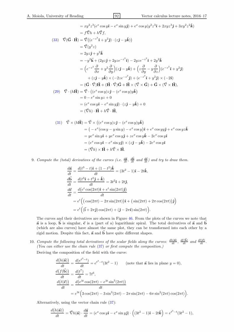
A. Moiola, University of Reading 92 Vector calculus lecture notes, 2016–17
= xy2z3(ex cos yı− ex sin y) + ex cos y(y2z3ı+ 2xyz3+ 3xy2z2k)
= f ~∇h+ h~∇f,(33) ~∇(~G · ~H) = ~∇
((e−z2
ı+ y2) · (z− yk))
= ~∇(y2z)
= 2yz+ y2k
= −y2~k+ (2yz+ 2yze−z2
ı)− 2yze−z2
ı+ 2y2k
=(e−z2 ∂
∂x+ y2
∂
∂y
)(z− yk) +
(z∂
∂y− y
∂
∂z
)(e−z2
ı+ y2)
+ (z− yk)× (−2ze−z2
) + (e−z2
ı+ y2)× (−2ı)
= (~G · ~∇)~H+ (~H · ~∇)~G+ ~H× (~∇× ~G) + ~G× (~∇× ~H),
(29) ~∇ · (h~H) = ~∇ ·((ex cos y)z− (ex cos y)yk
)
= 0− ex sin yz + 0
= (ex cos yı− ex sin y) · (z− yk) + 0
= (~∇h) · ~H+ h~∇ · ~H,
(31) ~∇× (h~H) = ~∇×((ex cos y)z− (ex cos y)yk
)
=(− ex(cos y − y sin y)− ex cos y
)ı+ ex cos yy+ ex cos yzk
= yex sin yı+ yex cos y+ zex cos yk − 2ex cos yı
= (ex cos yı− ex sin y)× (z− yk)− 2ex cos yı
= (~∇h)× ~H+ h~∇× ~H.
9. Compute the (total) derivatives of the curves (i.e. d~adt ,
d~bdt and d~c
dt ) and try to draw them.
d~a
dt=d(t3 − t)ı+ (1− t2)k
dt= (3t2 − 1)ı− 2tk,
d~b
dt=d(t3ı+ t2+ k)
dt= 3t2ı+ 2t,
d~c
dt=d(et cos(2πt)ı+ et sin(2πt)
)
dt
= et((
cos(2πt)− 2π sin(2πt))ı+
(sin(2πt) + 2π cos(2πt)
))
= et((~i+ 2π) cos(2πt) + (− 2πı) sin(2πt)
).
The curves and their derivatives are shown in Figure 46. From the plots of the curves we note that~a is a loop, ~b is singular, ~c is a (part of a) logarithmic spiral. The total derivatives of ~a and ~b(which are also curves) have almost the same plot, they can be transformed into each other by a
rigid motion. Despite this fact, ~a and ~b have quite different shapes.
10. Compute the following total derivatives of the scalar fields along the curves: dh(~a)dt , df(~b)
dt and dℓ(~c)dt .
(You can either use the chain rule (37) or first compute the composition.)
Deriving the composition of the field with the curve:
d(h(~a)
)
dt=d(et
3−t)
dt= et
3−t(3t2 − 1) (note that ~a lies in plane y = 0),
d(f(~b)
)
dt=d(t7)
dt= 7t6,
d(ℓ(~c)
)
dt=d(e3t cos(2πt)− e3t sin3(2πt)
)
dt
= e3t(3 cos(2πt)− 3 sin3(2πt)− 2π sin(2πt)− 6π sin2(2πt) cos(2πt)
).
Alternatively, using the vector chain rule (37):
d(h(~a)
)
dt= ~∇h(~a) · d~a
dt= (ex cos yı− ex sin y) ·
((3t2 − 1)ı− 2tk
)= et
3−t(3t2 − 1),

A. Moiola, University of Reading 93 Vector calculus lecture notes, 2016–17
−0.5 0 0.50
0.2
0.4
0.6
0.8
1
−1 0 10
0.2
0.4
0.6
0.8
1
−2 0 2 4−3
−2
−1
0
1
2
−1 0 1 2−2
−1
0
1
2
0 1 2 3−2
−1
0
1
2
−10 0 10 20−20
−10
0
10
20
xxx
xxx
yy
yy
z
z ~a(t) ~b(t) ~c(t)
d~a(t)/dt d~b(t)/dt d~c(t)/dt
Figure 46: The images of the three curves and of their total derivatives.
d(f(~b)
)
dt= ~∇f(~b) · d
~b
dt
=(y2z3ı + 2xyz3+ 3xy2z2k
)· (3t2ı+ 2t)
=(t4ı+ 2t5+ 3t7k
)· (3t2ı+ 2t)
= 7t6,
d(ℓ(~c)
)
dt= ~∇ℓ(~c) · d~c
dt
=((3x2 + y2 + z2)ı+ (2xy − 3y2)+ 2xzk
)
· et((
cos(2πt)− 2π sin(2πt))ı+
(sin(2πt) + 2π cos(2πt)
))
= e2t((
3 cos2(2πt) + sin2(2πt))ı+
(2 cos(2πt) sin(2πt)− 3 sin2(2πt)
))
· et((
cos(2πt)− 2π sin(2πt))ı+
(sin(2πt) + 2π cos(2πt)
))
= e3t(3 cos(2πt)− 3 sin3(2πt)− 2π sin(2πt)− 6π sin2(2πt) cos(2πt)
).
B.2 Exercises of Section 2
Solution of Exercise 2.4. We start by computing the total derivative of the curve and its magnitude:
d~aAdt
= − sin tı+ cos tı+ k,
∣∣∣∣d~aAdt
∣∣∣∣ =√(− sin t)2 + (cos t)2 + 12 =
√2.
The value of the field fA(~r) = x+ y + z along the curve is
fA(~aA(t)
)= cos t+ sin t+ t.
To conclude, we simply apply formula (36) for the line integral of a scalar field:
∫
ΓA
fA ds =
∫ 2π
0
fA(~aA(t)
)∣∣∣∣d~aAdt
∣∣∣∣dt =∫ 2π
0
(cos t+ sin t+ t)√2 dt =
(0 + 0 +
(2π)2
2
)√2 = 2
√2π2.
Similarly, for the two remaining integrals we have:∣∣∣∣d~aBdt
∣∣∣∣ =√1 + t4,
∫
ΓB
fB ds =
∫ 1
0
√(1 + t4)(t6 + t2) dt =
∫ 1
0
(t5 + t) dt =2
3,

A. Moiola, University of Reading 94 Vector calculus lecture notes, 2016–17
∣∣∣∣d~aCdt
∣∣∣∣ =√1 + t2 =
√1 + x2 + y2,
∫
ΓC
fC ds =
∫ 10
0
√t2
1 + t2
√1 + t2 dt =
∫ 10
0
t dt = 50.
Solution of Exercise 2.7. (1) We compute the length of the logarithmic spiral using the formula (43):
d~a
dt= e−t(− sin t− cos t)ı + e−t(cos t− sin t),
∣∣∣∣d~a
dt
∣∣∣∣ = e−t√sin2 t+ cos2 t+ 2 sin t cos t+ sin2 t+ cos2 t− 2 sin t cos t =
√2e−t,
length(Γa)(43)=
∫
Γa
ds =
∫ ∞
0
∣∣∣∣d~a
dt
∣∣∣∣ dt =∫ ∞
0
√2e−t dt = −
√2e−t
∣∣∣∞
0=
√2.
(2) To compute the length of the second spiral we can proceed directly:
d~b
dt=
−τ sin τ − cos τ
τ2ı +
τ cos τ − sin τ
τ2,
∣∣∣∣∣d~b
dt
∣∣∣∣∣ =1
τ2
√τ2 sin2 τ + cos2 τ + 2τ sin τ cos τ + τ2 cos2 τ + sin2 τ − 2τ sin τ cos τ =
√τ2 + 1
τ2,
length(Γb)(43)=
∫ ∞
1
∣∣∣∣∣d~b
dτ
∣∣∣∣∣ dτ =
∫ ∞
1
√τ2 + 1
τ2dτ =
(arsinhτ −
√τ2 + 1
τ
)∣∣∣∞
1= ∞− 1− arsinh1 +
√2 = ∞.
However the integral of√τ2+1τ2 , which we computed by parts, is not easy. A simpler way is to note that
the integrand satisfies the lower bound√τ2+1τ2 ≥ τ
τ2 = 1τ , thus
length(Γb) =
∫ ∞
1
√τ2 + 1
τ2dτ ≥
∫ ∞
1
1
τdτ = log τ
∣∣∣∞
1= ∞.
Thus the length of the path cannot be shorter than ∞.(3) Both curves are in the form F (t)(cos tı+sin t) for some positive function F , so they rotate around
the origin in anticlockwise direction with period 2π. Since both curves are defined for an unboundedparametrisation interval (i.e. t ≥ 0 and τ ≥ 1), they rotate infinitely many times: for all values t, τ = 2nπwith n ∈ N we have a2(t) = b2(τ) = 0 and a1(t), b1(τ) > 0 so the curves cross the positive x axis; for allvalues t, τ = (2n+ 1)π with n ∈ N we have a2(t) = b2(τ) = 0 and a1(t), b1(τ) < 0 so the curves cross thenegative x axis. This happens for all n ∈ N, so infinitely many times.
(4) We first note that ℓ must be at least 1, since no curve connecting ı and ~0 can be shorter than thestraight segment, which has length 1. The simplest way to construct ~c is to slightly modify the curve ~a.To guarantee infinitely many turns around the origin we keep the cos t and sin t terms. To modify thespeed of convergence to the origin, thus the length of the path, we modify the exponential term as e−λt,using a positive parameter λ. So we define a new curve ~c, depending on λ, and we compute its length:
~c(t) = e−λt cos tı+ e−λt sin t, t ∈ [0,∞),
d~c
dt= e−λt(− sin t− λ cos t)ı+ e−λt(cos t− λ sin t),
∣∣∣∣d~c
dt
∣∣∣∣ = e−λt√sin2 t+ λ2 cos2 t+ 2λ sin t cos t+ λ2 sin2 t+ cos2 t− 2λ sin t cos t =
√1 + λ2e−λt,
length(Γc)(43)=
∫ ∞
0
∣∣∣∣d~c
dt
∣∣∣∣ dt =∫ ∞
0
√1 + λ2 e−λt dt = −
√1 + λ2
λe−λt
∣∣∣∞
0=
√1 + λ2
λ=√1 + 1/λ2.
Thus to obtain a length ℓ we need to take√1 + 1/λ2 = ℓ, which gives λ = 1/
√ℓ2 − 1, which is acceptable
for any ℓ > 1. The desired curve is ~c(t) = e−t/√ℓ2−1 cos t ı+ e−t/
√ℓ2−1 sin t for t ∈ [0,∞).
Solution of Exercise 2.11. Proceeding as in Example 2.10 we obtain∫
ΓA
~G · d~aA =
∫
ΓB
~G · d~aB = −∫
ΓC
~G · d~aC =
∫
ΓD
~G · d~aD =
∫
ΓE
~G · d~aE =5
6.
Solution of Exercise 2.12. We first note that the position vector field evaluated on any curve equalsthe parametrisation of the curve itself: ~F(~a(t)) = ~a(t), thus
∫Γa
~F · d~r =∫Γa~a · d~a
dt ds. We report theparametrisation of the curves and their total derivatives, compute their scalar products and integrate:
~a(t) = e−t cos t ı+ e−t sin t , t ∈ [0,∞), ~b(τ) =1
τcos τ ı+
1
τsin τ , τ ∈ [1,∞),

A. Moiola, University of Reading 95 Vector calculus lecture notes, 2016–17
d~a
dt= e−t(− sin t− cos t)ı+ e−t(cos t− sin t),
d~b
dt=
−τ sin τ − cos τ
τ2ı+
τ cos τ − sin τ
τ2,
~a · d~adt
= e−2t(− sin t cos t− cos2 t+ cos t sin t− sin t sin t) = −e−2t,
~b · d~b
dt=
1
τ3(−τ sin τ cos τ − cos2 τ + τ cos τ sin τ − sin2 τ) = − 1
τ3,
∫
Γa
~F · d~r =∫
Γa
~a · d~adt
ds =
∫ ∞
0
−e−2t dt =e−2t
2
∣∣∣∣∞
0
= −1
2,
∫
Γb
~F · d~r =∫
Γa
~b · d~b
dτds =
∫ ∞
1
− 1
τ3dτ =
1
2τ2
∣∣∣∣∞
1
= −1
2.
Here we see a fact that might be surprising: the second spiral Γb has infinite length, as we have verifiedin Exercise (2.7), but the line integral of ~r along it is finite. This is because, when we approach the originproceeding along Γb, the field ~r becomes smaller and “more orthogonal” to the curve itself.
We could have guessed from the beginning the signs of the integrals. The position vector points in theradial direction away from the origin. The total derivatives of each curve instead point roughly towardsthe origin, as the magnitude of the curve points decreases monotonically with t. Thus the scalar products~F(~a) · d~a
dt and ~F(~b) · d~bdτ are negative, and the integrals of negative integrands are negative.
Solution of Exercise 2.17. We know the scalar potentials of the two vector fields considered: ~r =~∇(12 |~r|2) and zı+ xk = ~∇(xz). Applying the fundamental theorem of vector calculus (49) we have:
∫
Γ
~r · d~r = 1
2|~q|2 − 1
2|~p|2 =
1
2(3− 5) = −1, and
∫
Γ
(zı+ xk) · d~r = (−1)(−1)− (0)(2) = 1.
Solution of Exercise 2.20. We first need to find a parametrisation of the two paths41:
~a(t) = (1− t)ı+ t, 0 ≤ t ≤ 1, ~b(τ) = cos τ ı+ sin τ , 0 ≤ τ ≤ π/2.
The corresponding total derivatives are
d~a(t)
dt= −ı+ ,
d~b(τ)
dτ= − sin τ ı+ cos τ .
The line integrals are computed using the definition (44):
∫
Γa
~F · d~r =
∫ 1
0
~F(a1(t), a2(t)
)· d~a(t)dt
dt =
∫ 1
0
(a21(t) + a22(t)
)(ı+ 2) · (−ı+ ) dt
=
∫ 1
0
(1 + t2 − 2t+ t2
)(−1 + 2) dt = 1 +
1
3− 1 +
1
3=
2
3,
∫
Γb
~F · d~r =
∫ π/2
0
~F(b1(τ), b2(τ)
)· d~b(τ)
dτdτ =
∫ π/2
0
(cos2 τ + sin2 τ)(ı + 2) · (− sin τ ı+ cos τ ) dτ
=
∫ π/2
0
(− sin τ + 2 cos τ) dτ
= cosπ
2− cos 0 + 2 sin
π
2− 2 sin 0 = 0− 1 + 2− 0 = 1.
Since the values of the line integrals of ~F over two paths connecting the same endpoints are different fromone another (23 6= 1), by Theorem 2.19 (or by the equivalence in box (50)) the field ~F is not conservative.
Solution of Exercise 2.23.
∫∫
R
e3y sinxdxdy =
(∫ π
0
sinxdx
)(∫ 2
1
e3y dy
)=
(− cosx
∣∣∣∣π
0
)(e3y
3
∣∣∣∣2
1
)=
2
3(e6 − e3),
41How did we find these parametrisations? Many choices are possible, we look for the simplest one; see also Remark 1.24.We first look for the first component a1(t) of ~a(t). If we choose to parametrise Γa with the unit interval [0, 1], a1 must
be a scalar function such that a1(0) = 1 and a1(1) = 0: the easiest possible choice is a1(t) = 1− t. Since by definition of Γa
we have a1(t) + a2(t) = 1, we have 1− t+ a2(t) = 1 and thus a2(t) = t.For the second path, we can proceed similarly (see Example 2.3), but we would obtain a complicated parametrisation.
Instead, we note that we need two scalar functions b1 and b2 such that b21(τ) + b22(τ) = 1, so the most natural choice isb1(τ) = cos τ and b2(τ) = sin τ . For this choice, we need to fix the parametrisation endpoints to be τI = 0 and τF = π/2,
so that ~b(τI ) = ı and ~b(τF ) = .

A. Moiola, University of Reading 96 Vector calculus lecture notes, 2016–17
∫∫
Q
y dxdy =
∫ 5
0
(∫ 1
x5
y dy
)dx =
∫ 5
0
(1
2− x2
50
)dx =
5
2− 125
150=
5
3,
∫∫
S
cosxdxdy =
∫ π2
0
cosx
(∫ sin x
0
dy
)dx =
∫ π2
0
cosx sinxdx =
∫ π2
0
1
2sin(2x) dx =
− cos(2x)
4
∣∣∣∣
π2
0
=1
2.
Solution of Exercise 2.29. Proceeding as in Example 2.28, we have to compute the Jacobian deter-
minant ∂(ξLR,ηLR)∂(x,y) and integrate it over the unit square S = 0 < x < 1, 0 < y < 1:
J ~TLR =
(yexy cos(2πy) xexy cos(2πy)− 2πexy sin(2πy)yexy sin(2πy) xexy sin(2πy) + 2πexy cos(2πy)
),
∂(ξLR, ηLR)
∂(x, y)= 2πye2xy,
Area(RLR) = 2π
∫ 1
0
∫ 1
0
ye2xy dxdy = π
∫ 1
0
e2xy∣∣∣∣1
x=0
dy = π
∫ 1
0
(e2y−1) dy = π(e2y
2−y)∣∣∣∣
1
y=0
=π(e2 − 3)
2.
Solution of Exercise 2.30. (i) The domain is defined implicitly by the change of coordinates Q ∋xı+ y 7→ ξξ + ηη ∈ (0, 1)2. We compute the Jacobian determinant and the integral:
∂(x, y)
∂(ξ, η)= det
(4− η −ξ−η π − ξ
)= (4− η)(π − ξ)− ξη = 4π − 4ξ − πη;
Area(Q) =
∫∫
Q
1 dA =
∫∫
(0,1)2
∣∣∣∣∂(x, y)
∂(ξ, η)
∣∣∣∣dξ dη =
∫ 1
0
∫ 1
0
|4π − 4ξ − πη| dξ dη = 4π − 4
2− π
2=
7
2π − 2.
You can visualise this domain in Matlab/Octave using the function VCplotter.m (available on the courseweb page), with the command:VCplotter(6, @(x,y) x*(4-y), @(x,y) y*(pi-x),0,1,0,1);
(ii) We repeat the same computations done in part (i) with the general parameters:
∂(x, y)
∂(ξ, η)= det
(a− η −ξ−η b− ξ
)= (a− η)(b− ξ)− ξη = ab− aξ − bη;
Area(Qab) =
∫∫
Qab
1 dA =
∫∫
(0,1)2
∣∣∣∣∂(x, y)
∂(ξ, η)
∣∣∣∣dξ dη =
∫ 1
0
∫ 1
0
|ab− aξ − bη| dξ dη = ab− a+ b
2.
Alternative solution: Qab is the quadrilateral with vertices ~0, aı, (a− 1)ı+ (b− 1), b and straight edges,thus computing its area by decomposing it in the rectangle ~0, (a − 1)ı, (a − 1)ı + (b − 1), (b − 1), thetriangle (a− 1)ı, aı, (a− 1)ı+ (b− 1) and the triangle (b− 1), b, (a− 1)ı+ (b− 1) (so that the area is(a− 1)(b− 1) + 1
2 (a− 1 + b− 1) = ab− 12 (a+ b)) is also correct.
Solution of Exercise 2.31. We first compute the inverse change of variables, solving (60) for x and y:taking the sum and the difference of the two equations we have
ξ + η = 2y − 1,
ξ − η = 12x− 1,
⇒x = 2(ξ − η + 1),
y = ξ+η+12 .
(108)
The Jacobian determinant we will need in the integral is
∂(ξ, η)
∂(x, y)
(56)=
∂ξ
∂x
∂η
∂y− ∂ξ
∂y
∂η
∂x=
1
41− 1
(− 1
4
)=
1
2.
We call ~T the change of variables and R the counterimage of P , i.e.:
~T : R→ P, ~T(xı+ y) = ξ(x, y)ξ + η(x, y)η.
The domain P is a square, so we want to identify the four parts of the boundary of R correspondingto the four edges42 of P . For this purpose, it is enough to insert the equations of the edges of P either in(60) or in (108):
line connecting ξ, η : ξ + η = 1, y = 1,
line connecting η,−ξ : ξ − η = −1, x = 0,
line connecting − ξ,−η : ξ + η = −1, y = 0,
line connecting − η, ξ : ξ − η = 1, x = 4,
42If you don’t remember how to compute the equations of the straight lines defining the edges of P , draw the domain and
use four times the formula for the line through two points ~p = ξpξ + ηpη and ~q = ξq ξ+ ηq η:η−ηpηq−ηp
=ξ−ξpξq−ξp
. You have to
repeat this for each of the four edges. In this exercise all the coefficients are either 1, 0 or −1. See also Figure 47.

A. Moiola, University of Reading 97 Vector calculus lecture notes, 2016–17
so all the four lines are parallel to the axes in the xy-plane and the domain R is the rectangle R =(0, 4)× (0, 1) = xı+ y ∈ R2, 0 < x < 4, 0 < y < 1. Now we can compute the desired integral using thechange of variables formula (57):
∫∫
P
f(ξ, η) dξ dη(57)=
∫∫
R
f(x4+ y − 1, y − x
4
)∣∣∣∣∂(ξ, η)
∂(x, y)
∣∣∣∣dxdy
=
∫∫
R
e−x4−y+1−y+ x
41
2dxdy
=
∫ 1
0
(∫ 4
0
e−2y+1 1
2dx
)dy =
∫ 1
0
2e−2y+1 dy = 2e−2y+1
−2
∣∣∣∣1
0
= e− e−1 ≈ 2.35.
x
y
R
y = 0
y = 1
x = 0 x = 4ξ
η
Pξ + η = 1
ξ − η = 1
−ξ + η = 1
−ξ − η = 1
Figure 47: The rectangle R and the square P in Exercise 2.31.
Solution of Exercise 2.36. (i) We use the following change of variables (we write also the inverse):43
(I)
ξ = xy,
η = y,
(∂ξ∂x
∂ξ∂y
∂η∂x
∂η∂y
)=
(y x0 1
),
∂(ξ, η)
∂(x, y)= y,
x = ξ
η ,
y = η,
∂(x, y)
∂(ξ, η)=
1
η.
(ii) The integral is computed as:
∫∫
T
ξ
ηdξ dη
(57)=
∫∫
S
ξ(x, y)
η(x, y)
∣∣∣∣∂(ξ, η)
∂(x, y)
∣∣∣∣ dxdy =
∫∫
S
xy
yy dxdy =
∫ 1
0
xdx
∫ 1
0
y dy =1
2
1
2=
1
4.
43How did we find this transformation? First we decide how to change the domain geometrically: since we are transforminga square into a triangle, have to “get rid of” one of the sides of S, we choose to maintain the upper and the left side, collapsethe lower one and transform the right one into the diagonal (see below for other options). We then note that we canmaintain the vertical coordinate of every point and modify only the horizontal one, so we fix η = y. We want to modify xby multiplying with a suitable function, so ξ = xg(x, y). The function g must have value 1 on the horizontal line y = 1 (sothe upper side is preserved), and value 0 on the horizontal line y = 0 (so the lower side is collapsed). The choice g(x, y) = yis the easiest that satisfies these two conditions (g(x, 1) = 1, g(x, 0) = 0), so the candidate transformation is ξ = xy, η = y.
Then, we can immediately verify that, under this transformation, the upper side of S is preserved (y = 1 ⇒ η = 1), theleft side is preserved (x = 0 ⇒ ξ = 0), the right side is mapped into the diagonal side of T (x = 1 ⇒ ξ = η), the lower sideis collapsed to the origin (y = 0 ⇒ ξ = η = 0). Thus the transformation maps correctly the boundaries: ∂S → ∂T . It is
surjective (for all ξξ + ηη ∈ T , ξ/ηı+ η belongs to S), and it is injective in the interior of S:
~T(xA, yA) = xAyAξ + yAη = xByB ξ + yB η = ~T(xB , yB) ⇒ xAyA = xByB ,yA = yB ,
yA,yB>0⇒ xA = xB,yA = yB.
(The verification of the mapping of the boundary and the bijectivity was not required in the exercise, however it is what youshould do to check if your transformation is correct.)
Another smart way to obtain and verify the transformation, is to rewrite the domains as
T = 0 < ξ < η < 1 = 0 < ξ/η < 1, 0 < η < 1, S = 0 < x < 1, 0 < y < 1,
from which the inverse transformation x = ξη, y = η is immediate (this corresponds to the setting of Example 2.34).
Many other changes of variables are possible, some simple ones are
(II)
ξ = x,
η = x+ y − xy,(III)
ξ = 1
2x,
η = y + 12x,
for x+ y ≤ 1,
ξ = x+ 1
2(y − 1),
η = 12(y + 1),
for x+ y > 1.
The transformation (II) corresponds to that described in Example 2.33 for general y-simple domain; (III) is “piecewiseaffine” (and continuous). See a representation of the three transformations in Figure 48; you can play around with thesetransformations using VCplotter.m. Note that the transformation of the unit cube into a tetrahedron in equation (64) isvery similar to this exercise.

A. Moiola, University of Reading 98 Vector calculus lecture notes, 2016–17
We can double check the computation above using the iterated integral on T :
∫∫
T
ξ
ηdξ dη =
∫ 1
0
∫ η
0
ξ
ηdξ dη =
∫ 1
0
η2
2ηdη =
1
4.
S
x
y
ξ
η
(I)
ξ
η
(II)
ξ
η
(III)
Figure 48: The square S and its image T under the three transformation described in exercise (1); manyother options are possible. In each case, the point ~0, and ı + are mapped into ~0, η and ξ + η,respectively, while ı is mapped into the point denoted with the little circle. The continuous, dashed andgrey lines represent the images of the vertical, horizontal and diagonal segments in the first plot. Note thatthe first two transformations (which are polynomials of degree two) map some straight lines into parabolas,while the third one (which is piecewise affine) maps straight lines into polygonal lines.
Solution of Exercise 2.42. We only need to show that for all u,w ∈ R we have ~X(u,w) ∈ S, i.e.
X21 (u,w) +X2
2 (u,w) +X23 (u,w) = 1 and X3(u,w) 6= 1. We compute the magnitude of ~X(u,w):
|~X(u,w)|2 =u2 + w2 +
(u2
4 + w2
4 − 1)2
(1 + u2
4 + w2
4
)2 =u2 + w2 + u4
16 + w4
16 + 1− u2
2 − w2
2 + u2w2
8
1 + u4
16 + w4
16 + u2
2 + w2
2 + u2w2
8
= 1,
so ~X(u,w) belongs to the unit sphere. Since X3(u,w) = 1 reads u2
4 + w2
4 − 1 = 1 + u2
4 + w2
4 , which has
no solutions, no point is mapped to the north pole and we conclude that ~X maps into S.To compute the inverse of ~X, we have to solve ~X(u,w) = ~r for u and w. Using the relation x2 + y2 +
z2 = 1 between the components of a point in S, after some computations we find u = 2x/(1 − z) andw = 2y/(1− z).
Solution of Exercise 2.43. The surface is a torus, i.e. a “mathematical doughnut”. It can be describedas the set of points with distance b from a circle of radius a centred at the origin and lying in the xy-plane.You can see it in the left plot of Figure 49 for a = 3 and b = 1. To be more precise, S is the torus afterthe inner circle (corresponding to w = ±π) and the circle in the y = 0, x < 0 half plane (correspondingto u = ±π) have been deleted. The two deleted circles are highlighted in the figure.
-0.5
0
0.5
3
2
12
0
-1 0
-2-2
-3
0
1
0.2
0.8
0.4
0.6
0.6 1
0.8
0.4
0.50.2
0
0
Figure 49: Left: The torus described by the parametrisation in Exercise 2.43 with a = 3 and b = 1.Right: The “hump” graph surface of Exercise 2.45. The little coloured arrows represent the (scaled)tangent vectors. The black arrow is the (scaled) unit normal vector at 1/2ı+ 1/4+ 3/4k.

A. Moiola, University of Reading 99 Vector calculus lecture notes, 2016–17
Solution of Exercise 2.45. We have 0 ≤ g ≤ 1 in R with g(1/2, 1/2) = 1 and g = 0 on the boundaryof R, i.e. where either x or y are equal to 0 or 1. So its graph Sg looks like a “hump”, see the right plotof Figure 49.
The gradient of g is ~∇g = 16(1− 2x)y(1 − y)ı+ 16x(1− x)(1 − 2y). We can see Sg as a parametric
curve with chart ~Xg = xı+ y+ g(x, y)k defined on R, so∂~Xg
∂x = ı+ ∂g∂x k = ı+ 16(1− 2x)y(1− y)k and
∂~Xg
∂y = + ∂g∂y k = ı+ 16x(1− x)(1 − 2y)k. These are tangent vector fields to Sg.
Solution of Exercise 2.49.
∂ ~X
∂u= ı+ + k,
∂ ~X
∂w= ı− ,
∂ ~X
∂u× ∂ ~X
∂w= −ı+ − 2k,
∣∣∣∣∣∂ ~X
∂u× ∂ ~X
∂w
∣∣∣∣∣ =√6,
Area(S) =
∫∫
S
dS =
∫∫
R
∣∣∣∣∣∂ ~X
∂u× ∂ ~X
∂w
∣∣∣∣∣dA =
∫ 1
0
∫ 1
0
√6 du dw =
√6.
Since the chart is affine, S is the flat parallelogram with vertices ~X(0, 0) = ~0, ~X(1, 0) = ı + + k,~X(1, 1) = 2ı+k, ~X(0, 1) = ı−. Moreover, since two sides of this are perpendicular (i.e. (~X(1, 0)− ~X(0, 0))·(~X(0, 1)− ~X(0, 0)) = 0), this is a rectangle. The sides of this rectangle have length |~X(1, 0)− ~X(0, 0)| =
√3
and |~X(0, 1)− ~X(0, 0)| =√2, thus we have verified geometrically that the area of S is
√6.
Solution of Exercise 2.50. We simply integrate the field f = 1 over S using formula (69). Here theregion R is the unit square (0, 1)× (0, 1).
Area(S) =
∫∫
S
1 dS =
∫∫
(0,1)×(0,1)
√
1 +(∂(23x
32 + 2
3y32 )
∂x
)2+(∂(23x
32 + 2
3y32 )
∂y
)2dA
=
∫ 1
0
∫ 1
0
√1 + x+ y dy dx
=
∫ 1
0
2
3(1 + x+ y)
32
∣∣∣∣1
y=0
dx
=2
3
∫ 1
0
((2 + x)
32 − (1 + x)
32
)dx
=2
3
2
5
((2 + x)
52 − (1 + x)
52
)∣∣∣∣1
x=0
=4
15
(3
52 − 2
52 − 2
52 + 1
)=
4
15
(√243− 2
√32 + 1
)≈ 1.407.
Solution of Exercise 2.51. (i) This surface is not a graph, so we cannot use formula (68) but we needto use the more general (67). We compute the area element, by taking the partial derivatives of the
chart ~X, using the definition of the vector product ×, the definition of vector magnitude | · |, and thetrigonometric identity sin2 u+ cos2 = 1:
~X(u,w) = (a+ b cosw) cosuı+ (a+ b cosw) sin u+ b sinwk − π < u < π, −π < w < π,
∂ ~X
∂u= −(a+ b cosw) sin uı+ (a+ b cosw) cos u,
∂ ~X
∂w= −b sinw cosuı− b sinw sinu+ b coswk,
∂ ~X
∂u× ∂ ~X
∂w= b(a+ b cosw) cos u coswı + b(a+ b cosw) sinu cosw+ b(a+ b cosw) sinwk,
∣∣∣∣∣∂ ~X
∂u× ∂ ~X
∂w
∣∣∣∣∣ = b|a+ b cosw|(cos2 u cos2 w + sin2 u cosw +sin2 w)1/2 = b|a+ b cosw|.
Since 0 < b < a, we have a+ b cosw > 0 for all values of w, so we can write∣∣∣∂ ~X∂u × ∂~X
∂w
∣∣∣ = b(a+ b cosw).
The area of S is simply the surface integral of the constant field 1:
Area(S) =
∫∫
S
dS =
∫∫
R
∣∣∣∣∣∂ ~X
∂u× ∂ ~X
∂w
∣∣∣∣∣ dA

A. Moiola, University of Reading 100 Vector calculus lecture notes, 2016–17
=
∫ π
−π
∫ π
−π
b(a+ b cosw) du dw =
∫ π
−π
du
∫ π
−π
b(a+ b cosw) dw = (2π)(2πab) = 4π2ab.
Choosing a = 2 and b = 1 we have that the area is 8π2.(ii) To compute the integral of the scalar field f(~r) = (x2 + y2)−1/2 we need to evaluate f on S and
write it in terms of u and w. We use the chart ~X:
f(~X(u,w)
)=((a+ b cosw)2 cos2 u+ (a+ b cosw)2 sin2 u
)−1/2= |a+ b cosw|−1 = (a+ b cosw)−1,
∫∫
S
f dS(67)=
∫∫
R
f(~X)
∣∣∣∣∣∂ ~X
∂u× ∂ ~X
∂w
∣∣∣∣∣dA =
∫ π
−π
∫ π
−π
(a+ b cosw)−1 b(a+ b cosw) du dw = 4π2b.
Solution of Exercise 2.55. We use formula (74) together with the expression of ~F and g(x, y) = x2−y2:∫∫
S
~F · d~S =
∫∫
(0,1)×(0,1)
(− 0︸︷︷︸
=F1
∂(x2 − y2)
∂x− z(x, y)︸ ︷︷ ︸
=F2
∂(x2 − y2)
∂y+ (−y)︸ ︷︷ ︸
=F3
)dxdy
=
∫ 1
0
∫ 1
0
((y2 − x2)(−2y)− y
)dxdy =
∫ 1
0
(− 2y3 +
2
3y − y
)dy = −2
4+
1
3− 1
2= −2
3.
Solution of Exercise 2.56. Recall that in Exercise 2.45 we computed ~∇g = 16(1 − 2x)y(1 − y)ı +16x(1− x)(1 − 2y). The fluxes are
∫∫
Sg
~F · d~S (74)=
∫∫
R
(− ∂g
∂x+ 0 + 0
)dA =
∫ 1
0
∫ 1
0
16(2x− 1)y(1− y) dxdy
= 16
∫ 1
0
(2x− 1) dx
∫ 1
0
(y − y2) dxdy = 16(0)1
6= 0,
∫∫
Sg
~G · d~S (74)=
∫∫
R
(− x
∂g
∂x+ 0 + 0
)dA =
∫ 1
0
∫ 1
0
16x(2x− 1)y(1− y) dxdy
= 16
∫ 1
0
(2x2 − x) dx
∫ 1
0
(y − y2) dxdy = 161
6
1
6=
4
9.
To guess the signs of the fluxes we observe the shape of Sg in the right plot of Figure 49. The flux
of ~F can be understood as the “amount of vector field” passing through the surface and is defined as theintegral of the scalar product between ~F and the unit normal vector n, which points upwards as in (71).
The first field ~F = ı is constant (i.e. has the same value everywhere) and points in the x direction,
from the plot we see that n has positive x component only for x > 1/2 so ~F · n is positive for x > 1/2and negative for x < 1/2. Since Sg is symmetric with respect to the vertical plane x = 1/2, so it is n,and the contributions to the flux from ~r ∈ Sg, x < 1/2 and ~r ∈ Sg, x > 1/2 have the same absolutevalue and cancel each other. So the total flux is zero.
The second field ~G = xı points again in the x direction but is not constant. So the contribution to theflux from ~r ∈ Sg, x < 1/2 is again negative (because here ~F · n < 0) and that from ~r ∈ Sg, x > 1/2 is
positive. But now ~F is larger in this second portion of Sg, so the positive term is larger in absolute valuethan the negative one and the sum of the two terms is then positive.
What do you obtain if you make a similar reasoning for ~H = yı?
Solution of Exercise 2.57. We recall that we have:
~X = (a+ b cosw) cos uı+ (a+ b cosw) sin u+ b sinwk − π < u < π, −π < w < π,
∂ ~X
∂u× ∂ ~X
∂w= b(a+ b cosw) cosu coswı+ b(a+ b cosw) sin u cosw + b(a+ b cosw) sinwk.
The position vector has value equal to its argument, so ~r(~X(u,w)) = ~X(u,w). The flux is
∫∫
S
~r · d~S (73)=
∫∫
R
~r · ∂~X
∂u× ∂ ~X
∂wdA =
∫∫
R
~X · ∂~X
∂u× ∂ ~X
∂wdA
=
∫ π
−π
∫ π
−π
(b(a+ b cosw)2(cos2 u cosw + sin2 u cosw) + b2(a+ b cosw) sin2 w
)du dw
=
∫ π
−π
∫ π
−π
b(a+ b cosw)((a+ b cosw) cosw + b sin2 w
)du dw

A. Moiola, University of Reading 101 Vector calculus lecture notes, 2016–17
=
∫ π
−π
du
∫ π
−π
b(a+ b cosw)(a cosw + b) dw
= 2π
∫ π
−π
(ab2 + (a2b + b3) cosw + ab2 cos2 w
)dw = 2π
(2πab2 + πab2
)= 6π2ab2.
Solution of Exercise 2.65. The ellipsoid E = ~r ∈ R3 s.t. x2+y2+ z2
c2 < 1, in cylindrical coordinatesreads
E =
~r ∈ R3 s.t. r2 < 1− z2
c2
=
~r ∈ R3 s.t. r <
√1− z2
c2
.
Thus, it is a solid of revolution as in equation (83), with −c < z < c (the admissible interval for z
corresponds to the largest interval which guarantees 1− z2
c2 ≥ 0). From formula (84),
Vol(E) =
∫∫∫
E
dV = π
∫ c
−c
(1− z2
c2
)dz = π
(z − z3
3c2
)∣∣∣∣c
−c
=4
3πc.
Note that this result agrees with the formula for the volume of the sphere when c = 1.
Solution of Exercise 2.66. Using formula (84) it is easy to find Vol(B) = 1615π and Vol(F ) = π
2 .
Solution of Exercise 2.67. Using the computations already done in Example 2.62 we have:
Vol(D) =
∫∫∫
D
dV =
∫ π/2
−π/2
∫ π
−π
∫ (cos z)(2+sin 3θ)
0
r dr dθ dz
=1
2
∫ π/2
−π/2
(cos z)2 dz
∫ π
−π
(2 + sin 3θ)2 dθ =1
2
π
29π =
9π2
4.
You can plot the domain D in Matlab/Octave using the function VCplotter.m with the command:VCplotter(7, @(theta,z) (cos(z))*(2+sin(3*theta)), -pi/2, pi/2);
Solution of Exercise 2.68. We simply write the triple integrals in cylindrical coordinates using thevolume element (82). The Cartesian coordinates are written in the cylindrical system using (81).
∫∫∫
C
z dV =
∫ 1
0
∫ π
−π
∫ z
0
zr dr dθ dz =( ∫ π
−π
dθ)∫ 1
0
(z
∫ z
0
r dr)dz = 2π
∫ 1
0
zz2
2dz =
π
4;
∫∫∫
C
xdV(81)=
∫ 1
0
∫ π
−π
∫ z
0
(r cos θ)r dr dθ dz =( ∫ π
−π
cos θ dθ) ∫ 1
0
(∫ z
0
r2 dr)dz = 0
1
12= 0;
∫∫∫
C
(x2 + y2 + z2) dV(81)=
∫ 1
0
∫ π
−π
∫ z
0
(r2 cos2 θ + r2 sin2 θ + z2)r dr dθ dz
=
∫ 1
0
∫ π
−π
∫ z
0
(r2 + z2)r dr dθ dz
=( ∫ π
−π
dθ)∫ 1
0
(∫ z
0
(r3 + z2r) dr)dz = 2π
∫ 1
0
3
4z4 dz =
3π
10;
∫∫∫
C
g(z) dV =
∫ 1
0
∫ π
−π
∫ z
0
g(z)r dr dθ dz
=( ∫ π
−π
dθ)∫ 1
0
(g(z)
∫ z
0
r dr)dz = 2π
∫ 1
0
g(z)z2
2dz.
Solution of Exercise 2.71. We expand ~F using (81), (85) and the fundamental trigonometry equation:
~F = −yı+x+k = −(r sin θ)(cos θr−sin θθ)+(r cos θ)(sin θr+cos θθ)+z = r(sin2 θ+cos2 θ)θ+z = rθ+z.
From (86), its divergence is ~∇ · ~F = ∂0∂r + 1
r0 +1r∂r∂θ + ∂1
∂z = 0, thus ~F is solenoidal.

A. Moiola, University of Reading 102 Vector calculus lecture notes, 2016–17
Solution of Exercise 2.77.∫∫∫
B
f dV =
∫ π
−π
∫ π
0
∫ 1
0
ρ4(sin2 φ+ cos 12θ) ρ2 sinφdρ dφdθ
=( ∫ 1
0
ρ6 dρ)∫ π
0
∫ π
−π
(sin2 φ+ cos 12θ) sinφdθ dφ
=1
7
∫ π
0
2π sin3 φdθ dφ =2π
7
cos 3t− 9 cos t
12
∣∣∣∣π
0
=8π
21.
Solution of Exercise 2.79. We first convert the coordinates from degrees to radians. Denoting ϕ thelatitude, the colatitude is φ = π
2 − ϕ.
ϕS = 37 =2π
36037 ≈ 0.646, ϕN = 41 =
2π
36041 ≈ 0.716,
φS =π
2− ϕS = 0.925, φN =
π
2− ϕN = 0.855,
θE = −10203′ = − 2π
360
(102 +
3
60
)≈ −1.781, θW = −10903′ = − 2π
360
(109 +
3
60
)≈ −1.903,
(where the minus signs come from the fact that θ measures the longitude in the East direction).Placing the origin of the axis in the Earth’s centre, Colorado can be represented as the surface S =
~r, ρ = R = 6371, θW ≤ θ ≤ θE , φS ≤ φ ≤ φN, so its area is
Area(S) =
∫∫
S
1 dS =
∫ θE
θW
∫ φS
φN
R2 sinφdφdθ = (θE − θW )R2(− cos(φS) + cos(φN )
)≈ 269,305 km2,
which roughly agree with the value 269,837 km2 found on Wikipedia.
B.3 Exercises of Section 3
Solution of Exercise 3.7. We compute left- and right-hand sides of (96), and verify they coincide:
~∇× ~F = k, ⇒ left-hand side =
∫∫
R
(~∇× ~F)3 dA =
∫∫
R
1 dA = Area(R) = 4π,
~a(t) = 2 cos tı+ 2 sin t,d~a
dt(t) = −2 sin tı+ 2 cos t, 0 ≤ t ≤ 2π,
~F(~a(t)
)= (2 cos t+ 4 sin t)(ı + 3),
~F(~a(t)
)· d~adt
(t) = 4(cos t+ 2 sin t)(− sin t+ 3 cos t) = 4(3 cos2 t− 2 sin2 t+ 5 cos t sin t),
= 2(3(cos 2t+ 1)− 2(1− cos 2t) + 5 sin 2t
)= 2(5 cos 2t+ 1 + 5 sin 2t
),
∮
∂R
~F · d~r =
∫ 2π
0
~F(~a(t)
)· d~adt
(t) dt
=
∫ 2π
0
2(5 cos 2t+ 1 + 5 sin 2t
)dt = 2
(5
2sin 2t− 5
2cos 2t+ t
)∣∣∣∣2π
0
= 4π.
Solution of Exercise 3.8. Since the domain R is y-simple, we compute the double integral at theleft-hand side of (96) as an iterated integral:
∫∫
R
(~∇× ~F
)3dA
(23)=
∫∫
R
(−2y) dA(53)=
∫ 2
−2
(∫ √1− x2
4
0
(−2y) dy
)dx
=
∫ 2
−2
(− 1 +
x2
4
)dx = 2
(− 2 +
8
12
)= −8
3.
The boundary of R is composed of two parts. The horizontal segment −2 < x < 2, y = 0 does not give
any contribution to the line integral at the right-hand side of (96), since ~F vanishes on the x axis. Theupper arc is parametrised by the curve ~a(t) = 2 cos tı + sin t for 0 < t < π (recall that it needs to beoriented anti-clockwise), whose total derivative is d~a
dt (t) = −2 sin tı+ cos t. So the line integral reads:∮
∂R
~F · d~r =
∫
∂R∩y>0~F · d~r

A. Moiola, University of Reading 103 Vector calculus lecture notes, 2016–17
(44)=
∫ π
0
y2ı · (−2 sin tı+ cos t) dt
=
∫ π
0
−2y2 sin t dt (now use y = a2(t) = sin t on ∂R ∩ y > 0)
=
∫ π
0
−2 sin3 t dt =
∫ π
0
(2 sin t cos2 t− 2 sin t) dt =(− 2
3cos3 t+ 2 cos t
)∣∣∣∣π
0
= −8
3,
and we have proved that the right- and the left-hand sides of formula (96) are equal to each other, for this
choice of domain R and field ~F.
Solution of Exercise 3.12. k × n = k × (τ × k)(4)= τ (k · k)− k(τ · k) = τ1− k0 = τ .
Solution of Exercise 3.16. We compute the divergence ~∇ · ~F = ex +1 and the iterated triple integral:
∫∫
∂D
~F · d~S (101)=
∫∫∫
D
~∇ · ~F dV =
∫ 1
0
∫ 1
−1
∫ 10
0
(ex + 1) dz dy dx = 20 e.
Solution of Exercise 3.17. We want to find a vector field ~F defined in the ball B = |~r| ≤ R such
that ~F · n = x2 + y2 on S = ∂B. The outward-pointing unit vector field n on ∂B is n = r = 1R~r, so a
suitable vector field is ~F = Rxı +Ry. Thus we conclude:
∫∫
S
(x2 + y2) dS =
∫∫
S
~F · d~S (101)=
∫∫∫
B
~∇ · ~F dV =
∫∫∫
B
2R dV = 2RVol(B) =8
3πR4.
Solution of Exercise 3.18. We first decompose the boundary ∂C in the disc B = x2 + y2 < 1, z = 1and in the lateral part L = x2 + y2 = z2, 0 < z < 1. We need to find a vector field ~F such that~∇ · ~F = |~r|2 and ~F · n is “easy to integrate” on ∂D. Since the divergence must be a polynomial of degreetwo, the easiest choice is to look for a field whose components are polynomials of degree three. Moreover,the position field ~r has zero normal component on the lateral boundary L of C (draw a sketch to figure out
why), so a good ~F may be a multiple of ~r. It is easy to figure out that a possible candidate is ~F = 15 |~r|2~r,
whose divergence is |~r|2, as desired. From the divergence theorem we have:
∫∫∫
C
|~r|2 dV =
∫∫∫
C
~∇ · ~F dV(101)=
∫∫
∂C
~F · d~S
=
∫∫
B
~F · n︸︷︷︸=k
dS +
∫∫
L
~F · n︸ ︷︷ ︸=0
dS
=
∫∫
B
1
5(x2 + y2 + z2)z dS
=
∫∫
B
1
5(r2 + 1) dS using z = 1 on B and cylindrical coordinates
=1
5
∫ π
−π
(∫ 1
0
(r2 + 1)r dr
)dθ =
1
52π
(1
4+
1
2
)=
3π
10,
which agrees with the result found in Exercise 2.68.
Solution of Exercise 3.19. (i) We compute the divergence and integrate in spherical coordinates:
~∇ · ~F = x2 + z2 + y2 = |~r|2 = ρ2,∫∫
∂B
~F · d~S =
∫∫∫
B
~∇ · ~F dV =
∫∫∫
B
ρ2 ρ2 sinφdρ dφdθ =
∫ π
−π
dθ
∫ π
0
sinφdφ
∫ 1
0
ρ4 dρ = 2π 21
5=
4
5π.
(ii) Similarly, we find the flux through the boundary of CL = (0, L)3 integrating in Cartesian coordinates:
∫∫
∂CL
~F· d~S =
∫∫∫
CL
~∇ · ~F dV =
∫ L
0
∫ L
0
∫ L
0
(x2 + y2 + z2) dz dy dx
=
∫ L
0
∫ L
0
(Lx2 + Ly2 +1
3L3) dy dx =
∫ L
0
(L2x2 +1
3L4 +
1
3L4) dx =
1
3(L5 + L5 + L5) = L5.
Thus, the two fluxes are equal if L5 = 45π, i.e. if L = (45π)
15 ≈ 1.202.

A. Moiola, University of Reading 104 Vector calculus lecture notes, 2016–17
Solution of Exercise 3.23. The gradient of the field is ~∇f = yzı+xz+xyk, from which we computethe triple integral
∫∫∫
D
~∇f dV =
∫ 1
0
∫ 1
0
∫ 1
0
(yzı+ xz+ xyk) dxdy dz
= ı
∫ 1
0
1 dx
∫ 1
0
y dy
∫ 1
0
z dz +
∫ 1
0
xdx
∫ 1
0
1 dy
∫ 1
0
z dz + k
∫ 1
0
xdx
∫ 1
0
y dy
∫ 1
0
1 dz =1
4(ı+ + k).
The field f vanishes on the three faces of D incident to the origin (for example the lower face belongs tothe plane z = 0, so f(~r) = xy0 = 0). In the upper face z = 1 and n = k, thus the contribution of thisface to the surface integral at the right-hand side of (102) is
∫ 1
0
∫ 1
0
xy1k dy dx =1
4ı.
Similarly, from the faces lying in the planes x = 1 and y = 1 we have the contributions 14 ı and 1
4 ,respectively. The sum of the three contributions give the value of the triple integral computed above.
Solution of Exercise 3.24. We recall that harmonic means that ∆f = 0 (Section 1.3.4), and the
normal derivative is ∂f∂n = n · ~∇f . Taking g = f in Green’s first identity, we see that
∫∫∫
D
|~∇f |2 dV =
∫∫∫
D
~∇f · ~∇f dV = −∫∫∫
D
f ∆f︸︷︷︸=0
dV +
∫∫
∂D
f∂f
∂n︸︷︷︸=0
dS = 0.
Since the scalar field |~∇f |2 is non-negative (|~∇f(~r)|2 ≥ 0 for all ~r ∈ D), this equation implies that~∇f = ~0 everywhere in D. (More in detail, if ~∇f 6= ~0 was true in a portion of D, this would imply that
|~∇f |2 > 0 gave a positive contribution to the integral∫∫∫
D|~∇f |2 dV that can not be cancelled by negative
contributions from other parts of the domain as |~∇f |2 is never negative, so the integral in the formulaabove could not vanish.) Since the gradient of f vanishes, all the partial derivatives of f are zero, so fcan not depend on any of the variables x, y and z, which means it is constant.
Solution of Exercise 3.20. We first note that the vector field ~F := ~r/|~r|3 is well-defined in all of R3
except at the origin. We also know from Exercise 1.62 that ~∇ · ~F = ~0 in all points ~r 6= ~0. Thus, fromdivergence theorem we immediately conclude for the case ~0 /∈ D:
∫∫∂D
~r|~r|3 · d~S =
∫∫∫D~∇ · ~r
|~r|3 dV =∫∫∫D0 dV = 0.
On the other hand, if ~0 ∈ D we cannot apply directly the divergence theorem to ~F because this fieldis not defined at the origin. We denote by B a ball centred at ~0 and contained in D (it exists because Dis open) and we call R its radius. The outward-pointing unit normal vector on ∂B is nB(~r) = ~r/|~r|, so
∫∫
∂B
~F · d~S =
∫∫
∂B
~F · nB dS =
∫∫
∂B
~r
|~r|3 · ~r|~r| dS =
∫∫
∂B
1
R2dS =
Area(∂B)
R2=
4πR2
R2= 4π.
We now apply the divergence theorem in D\B, where ~F is well-defined and ~∇·~F = 0. So we have that the
flux of ~F through the boundary of D \B vanishes. The boundary of this set is made of two components:
∂D, which gives the integral we want to compute, and ∂B, for which we have just computed the flux of ~F.We need to be careful with the signs: on ∂B, the vector field nB we have used above is outward-pointingfor B, so inward-pointing for D \ B, so the outward-pointing vector for D \ B satisfies n = −nB. Informulas:
0 =
∫∫∫
D\B~∇ · ~F dV =
∫∫
∂(D\B)
~F · d~S =
∫∫
∂D∪∂B
~F · d~S =
∫∫
∂D
~F · d~S+
∫∫
∂B
~F · d~S
=
∫∫
∂D
~F · d~S+
∫∫
∂B
~F · (−nB) dS =
∫∫
∂D
~F · d~S− 4π,
which gives∫∫
∂D~F · d~S = 4π. (This is sometimes called Gauss’ theorem.)

A. Moiola, University of Reading 105 Vector calculus lecture notes, 2016–17
Solution of Exercise 3.30. As usual, we parametrise the unit circumference ∂S with the curve ~a(t) =cos tı+ sin t, 0 < t < 2π. The circulation in (106) reads
∮
∂S
~F · d~r =∫ 2π
0
((2x− y)ı− yz2− y2zk
)· (− sin tı+ cos t) dt
=
∫ 2π
0
(−2 cos t sin t+ sin2 t) dt since on ∂S x = cos t, y = sin t, z = 0,
=
∫ 2π
0
(− sin 2t+
1
2(1− cos 2t)
)dt = π.
The curl of ~F is ~∇ × ~F = k and the surface S is the graph of the field g(x, y) =√1− x2 − y2 over the
disc R = xı + y, x2 + y2 < 1. Thus, using formula (74) for the flux through a graph surface, we have
∫∫
S
(~∇× ~F) · d~S (74)=
∫∫
R
(− (~∇× ~F)1
∂g
∂x− (~∇× ~F)2
∂g
∂y+ (~∇× ~F)3
)dA
=
∫∫
R
(0 + 0 + 1) dA = Area(R) = π,
and both sides of (106) give the same value.
Solution of Exercise 3.31. The desired integral is the circulation of the field |~r|2ı along the boundary ofthe paraboloid S, so we apply Stokes’ theorem and exploit the computation already done in Exercise 2.55:
∮
∂S
|~r|2 dx (46)=
∮
∂S
|~r|2 ı · d~r (106)=
∫∫
S
(~∇× (|~r|2ı)
)· d~S (31)
=
∫∫
S
2(~r× ı) · d~S Ex. 2.55= −4
3.
Solution of Exercise 3.32. We can prove the assertion in two different ways. The first option is touse Stokes’ theorem to transform the line integral to a surface integral, then to use the product rule forthe curl, and to verify that the terms obtained are zero:
∮
∂S
f ~∇f · d~r (106)=
∫∫
S
~∇× (f ~∇f) · d~S (31)=
∫∫
S
(~∇f × ~∇f︸ ︷︷ ︸
=~0, (~u×~u=~0)
+f ~∇× ~∇f︸ ︷︷ ︸=~0, (26)
)· d~S = 0.
Alternatively, we can use the chain rule to reduce the desired integral to the line integral of a gradient,which vanishes by the fundamental theorem of vector calculus since the path of integration is a loop:
∮
∂S
f ~∇f · d~r (14)=
1
2
∮
∂S
~∇(f2) · d~r (49)= 0.
A. Moiola, University of Reading 106 Vector calculus lecture notes, 2016–17
C Further exercises for tutorials and personal revision
Some of these exercises will be solved in the tutorials. Which exercises you should try to solve before eachtutorial will be announced in the lectures.
Exercises for Section 1.
Exercise C.1. (Exercise 4 in assignment 1 of MA2VC 2013–14.) Show that, for any unit vector n, and anyvector ~w perpendicular to n, the identity
n× (n× ~w) = −~w
holds true. You can make use of the identities in Section 1.1. Demonstrate this identity for the vectors
n =3
5ı+
4
5k, ~w = 3.
Exercise C.2. Compute and draw the level sets of the scalar field f(~r) = xey.
Exercise C.3. Draw some paths of the curves
~a(t) = (λ + t2)ı+ t, ~b(t) = tı+ (λt− λ2), ~c(t) = t cos(t+ λ)ı + t sin(t+ λ)
for different values of λ ∈ R. Are they level sets of any scalar field?
Exercise C.4. Let u and w be two unit vectors orthogonal to each other. Show that the curve ~a(t) =u cos t+ w sin t lies on the unit sphere for all t ∈ R. Which curve is this?
Exercise C.5. Draw the path of the curve
~a(t) =(cos t− sin t)ı+ (cos t+ sin t)
| cos t|+ | sin t| , 0 ≤ t ≤ 2π.
Exercise C.6. Find a quotient rule for the gradient, i.e. give a formula for ~∇(f/g) where f and g 6= 0 arescalar fields. Hint: use parts 2 and 3 of Proposition 1.33.
Exercise C.7. • Compute the vector field n of unit length defined on the sphere of radius R > 0, which isorthogonal to the sphere itself and points outwards. (This is called “outward-pointing unit normal vectorfield”.) Hint: use part 4 of Proposition 1.33.
• Compute the outward-pointing unit normal vector field on the boundary of the parabolic “cup”x2 + y2 < z < 1.
Exercise C.8. • Fix ~F = exyz ı. Show that ~F and ~∇× ~F are orthogonal to each other at each point of R3.
• Prove that any vector field with only one non-zero component is orthogonal to its own curl.
• Find a vector field that is not orthogonal to its own curl.
Exercise C.9. Find a scalar field f defined on the complement of the x axis, whose direction of maximalincrease is (~r− xı)/(y2 + z2)1/2.
Exercise C.10. (Exercises 1–2 in assignment 1 of MA2VC 2013–14.) Prove the following identity:
~∇ ·(~rfg
)= 3fg + (~r · ~∇f)g + (~r · ~∇g)f,
where ~r = xı + y+ zk is the position vector, and f(~r) and g(~r) are two scalar fields.Hint: you can either use the vector differential identities in the boxes of Propositions 1.52 and 1.55, or thedefinitions of gradient and divergence.
Demonstrate the above identity for the scalar fields f = exy and g = y4z.
Exercise C.11. Prove identity (34) in the notes (curl of a vector product).
Exercise C.12. • Find a vector field ~F such that: ~F is irrotational, ~F is not solenoidal, all its streamlines(recall caption to Figure 7) are straight lines passing through the origin.
This last condition means that ~F(~r) is parallel to ~r in all points ~r 6= ~0.
• [Harder!] Find a vector field ~G (defined on a suitable domain) such that: ~G is solenoidal, ~G is notirrotational, all its streamlines are straight lines passing through the origin.

A. Moiola, University of Reading 107 Vector calculus lecture notes, 2016–17
Exercise C.13. Compute the total derivative of the field f(~r) = (x2 + y2)β , for β ∈ R, evaluated along the
curve ~a(t) = cos 2πtı+ sin 2πt+ e−t2 k.Interpret the result geometrically.
Exercise C.14. Let F : (0,∞) → R be a smooth function. Let f : R3 \ ~0 → R be the scalar field definedby f(~r) = F (|~r|).
• Compute ~∇f .
• Prove that ∆f = F ′′(|~r|) + 2F ′(|~r|)|~r| . Hint: use one of the identities of Section 1.4.
Exercise C.15. Let ~F : R3 → R3 be a conservative force field, i.e. a conservative field with ~F = −~∇ψ, wherethe scalar field ψ is the potential energy. Let a particle of mass m move with trajectory ~a(t) according to
Newton’s law ~F(~a(t)) = md2~adt2 (t) (force equals mass times acceleration). Define the kinetic energy of the
particle T (t) = 12m∣∣d~adt (t)
∣∣2. Prove that the total energy E(t) = ψ(~a(t)) + T (t) of the particle is constant intime.
Hint: you only need to use chain and product rule for the total derivative.
Exercises for Section 2.
Exercise C.16. Consider the curve ~a(t) = t cos t ı + t sin t for t ∈ [0, 4π] and the scalar field f(~r) =1/√1 + |~r|2. Draw the path Γ of the curve, compute the line integral
∫Γ f ds and the total derivative of f
evaluated along ~a.
Exercise C.17. Compute the line integral of the vector field ~F(~r) = y2ı + 2xy along the five curves ofExample 2.10.
Exercise C.18. Compute the integral of the scalar field f = x+ y on the square Q with vertices ı, ,−ı,−.
Exercise C.19. Compute the area of the “eye” domain xı+ y, 1− y2 < |x| < 2(1− y2).Hint: draw a sketch of the domain. This domain is neither y-simple nor x-simple, to compute the double
integral you need to use two of the fundamental properties of integrals in list (40) in the notes.
Exercise C.20. Compute the area of ~T(R), where R = xı + y, 0 < x < 1, 0 < y < 1 and ~T(x, y) =(x+ y)ξ + y3η.
Exercise C.21. Find a change of variables from the trapezoid R with vertices −2ı, 2ı, ı + ,−ı + to thesquare Q with vertices ~0, ξ, ξ + η, η.
Use the change of variables you have found to compute∫∫
Re(2−y)2 dxdy.
Exercise C.22. Let S be the surface parametrised by the chart ~X(u,w) = uı + wu + wk defined over the
triangular region R = 0 < w < u < 1. Compute the flux through S of the field ~F = + 2xk.
Rewrite the surface as the graph of a scalar field g(x, y) over a suitable region R and compute again thesame flux using formula (74).
Exercise C.23. Compute the triple integral of f = x2 + y2 over the domain D lying inside the ball of radiusa > 0 centred at the origin and above the cone z =
√x2 + y2.
Exercise C.24. Compute the area of the region bounded by ~a(t) = t(2π − t)(cos tı+ sin t), 0 ≤ t ≤ 2π.
Exercise C.25. London and Astana (Kazakhstan) approximately lie on the parallel 51N , and have longitude0 and 71E, respectively. Describe the location of the two cities in a suitable special coordinates system.Compute the distance between the two cities, if the distance is measured:
(i) along a straight (underground) segment,
(ii) on the Earth surface along the parallel 51N ,
(iii) along the shortest surface path.
Assume that Earth is a sphere of radius 6371 km.
Exercises for Section 3.
Exercise C.26. Compute the area of the region bounded by the curve ~a(t) = sin tı+ sin 2t, 0 ≤ t ≤ 2π.
Exercise C.27. Compute the flux of ~F = xyı + yz+ zxk through the boundary of the cube C = (0, 2)3 =0 < x, y, z < 2.
A. Moiola, University of Reading 108 Vector calculus lecture notes, 2016–17
Exercise C.28. Demonstrate the divergence theorem for ~F = 12z
2k and the upper half unit ball B = z >0, |~r| < 1.
Exercise C.29. Let ~F be a vector field, and a and ǫ be two positive numbers such that ~F(~r) · ~r ≥ ǫ for all
~r ∈ R3 with |~r| = a. Prove that ~F is not solenoidal in the ball B of radius a centred at the origin.
Exercise C.30. Prove the following “integration by parts formula” for the curl: given a domain D ⊂ R3 andtwo vector fields ~F, ~G,
∫∫∫
D
(~∇× ~F) · ~G dV =
∫∫∫
D
~F · (~∇× ~G) dV +
∫∫
∂D
(~G× n) · ~F dS.
Exercise C.31. Demonstrate Stokes’ theorem for the field ~F = zyı and the quadrilateral S with verticesı, ı+ 1
2 − k, , 2k.
Exercise C.32. Consider the field ~G = 2x2y2z− 2x2yz2k and a triangle T with the three vertices on the x-,y- and z-axis, respectively. Show that the flux of ~G through T is zero.
Exercise C.33. Use Stokes’ theorem to compute the flux of ~G = xı+y−2zk through the cylindrical surfaceS = x2 + y2 = 1, 0 < z < H, where H > 0.
D Alphabetical index
∆ (Laplacian), 17· (scalar product), 3∂(ξ,η)∂(x,y)(Jacobian determinant), 46∂(ξ,η,σ)∂(x,y,z) (Jacobian determinant, 3D), 53
∂D (boundary of a domain), 57∂S (boundary of a surface), 59× (vector product), 4~∆ (vector Laplacian), 17~F · ∇ (advection operator), 23~∇ (nabla symbol), 13~∇· (divergence), 18~∇× (curl operator), 19~F · ∇ (advection operator), 19∫∫∫
D f dV , 52∫∫Rf dA, 42∫∫
Sf dS, 53∫
Γ~F · d~r, 35∫
Γf ds, 31∫∫∂D
(integral on closed surfaces), 58∮(contour integral, circulation), 32, 35
Additivity of integrals, 31Advection operator
for scalar fields, 19for vector fields, 23
Arc length, 27Azimuth, 64
Boundary, 57Bounded domain, 69
Canonical basis, 2Chain rule
for gradient, 14, 28for partial derivatives, 13, 28for total derivative, 27
Chart, 54Circulation, 35Closed set, 6
Colatitude, 64Connected domain, 69Conservative field, 25Contour integral, 32curl operator, 19Curve, 9Cylindrical coordinates, 62
∂∂x (partial derivative), 12∂∂u (directional derivative), 13∂∂n ,
∂∂n (normal derivative), 13
Del, 13Direction (of a vector), 2Directional derivative, 13Divergence, 18Domain, 6Double integral, 42
Field line, 9Flux, 58Fundamental theorem of vector calculus, 39
Gradient, 13Graph surface, 8, 55
H~F (Hessian), 17Helmholtz decomposition, 26Hessian, 17
ı (first canonical unit vector), 2Induced orientation, 59Intrinsic parametrisation of a curve, 27Irrotational field, 25Iterated integral, 44
J~F (Jacobian matrix), 16 (second canonical unit vector), 2Jacobian determinant, 46Jacobian matrix, 16
k (third canonical unit vector), 2
Laplacian, 17

A. Moiola, University of Reading 109 Vector calculus lecture notes, 2016–17
Length (of a vector), 2Length of a path, 34Level line, level surface, 8Line integral
of scalar fields, 31of vector fields, 35
Linearityof differential operators, 20of gradient, 14of integrals, 31of partial derivatives, 13of the total derivative, 27
Longitude, 64Loop, 9
Magnitude (of a vector), 2
Nabla, 13Normal derivative, 13, 77
Open set, 6Oriented path, 36Oriented surface, 56
Parametric surface, 54Parametrisation
of a curve, 9of a surface, 54
Partial derivative, 12Path, 9Piecewise smooth domain, 68Polar coordinates, 60Position vector, 3Product rule
for partial derivatives, 13for the gradient, 14
for the total derivative, 27for vector differential operators, 22
~r (position vector), 3Region, 7Riemann sum, 33
Scalar field, 7Scalar potential, 25Scalar product, 3Second order partial derivatives, 16Simply connected domain, 26, 69Solenoidal field, 25Solid of revolution, 63Spherical coordinates, 64Star-shaped domain, 39, 61, 66Streamline, 9Surface, 54Surface area, 56Surface integral, 53, 55
τ (unit tangent vector to a curve), 36Total derivative, 26Triple integral, 52Triple product, 5
Unit normal to a surface, 15, 56Unit normal to a two-dimensional region, 73Unit tangent vector to a curve, 36
Vector field, 9Vector Laplacian, 17Vector potential, 25Vector product, 4
y-simple domain, 42
E References
[1] R.A. Adams, C. Essex, Calculus, a complete course, Pearson Canada, Toronto, 7th ed., 2010.UoR library call number: FOLIO–515-ADA.
[2] E. Carlen, Multivariable Calculus, Linear Algebra and Differential Equation, lecture notes, 2013,available on: http://www.math.rutgers.edu/~carlen/291F14/index.html.
[3] M. Corral, Vector Calculus, 2013, available on: http://www.mecmath.net/.
[4] O. Knill, http://www.math.harvard.edu/~knill/teach/index.html. Here you can find plenty ofmaterials: lecture notes, exercises and instructive illustrations. Click on one of the Math(s)21a links.
[5] S. Lang, Calculus of Several Variables, Springer Undergraduate Texts in Mathematics, 3rd ed., 1996.
[6] C.J. Smith, Vector Calculus Primer, 2011, Reading, available on Blackboard and on course web page.
[7] M. Spiegel, S. Lipschutz, D. Spellman, Vector Analysis, McGraw-Hill, 2nd ed., 2009.

A. Moiola, University of Reading 110 Vector calculus lecture notes, 2016–17
F Common errors in vector calculus
This is a list of errors I found dozens of times in previous vector calculus assignments and exams. Manyof them are trivial and can easily be avoided, nonetheless they appear too often, watch out!
• The most common source of mistakes is treating scalar quantities as vector ones and vice versa. E.g.summing or equating scalars to vectors, writing the divergence of a scalar field, evaluating fields at anumber and curves at a vector. One of the main aims of this module is to learn how to manipulatethese objects, so take the greatest care to avoid these mistakes! Remember: never confuse scalarswith vectors.
• An unbelievably large number of errors happen because brackets are not used or are badly placed.Typical example: instead of ∂
∂x (fg) you write ∂∂xfg, in the next line you have forgotten that also g
was inside the derivation and you go on with ∂f∂xg, which is wrong. When in doubt, always write the
brackets.
• You should know very well that the signs “=”, “⇐⇒” and “⇒” cannot be used in place of eachother. The equal sign can only stay between two numbers, vectors, sets, matrices, or any two othercomparable mathematical objects. The implication ⇒ and the double implication ⇐⇒ (“if and onlyif”) stay between two propositions, statements or equations (in which case they contain an equal sign).
• Whenever you use a mathematical object denoted by a certain letter for the first time in an exercise,you must introduce it, unless it is known from a standard definition (or from the statement of theexercise). E.g. the number π and the position vector ~r do not need to be defined every time and you
can use them directly; fields, curves, domains f, g, ~F, ~a, D . . . are not standard and you need to definethem. Examples of typical correct sentences: “given a scalar field f . . . ”, “let D ⊂ R3 be a domain. . . ”,“fix ~a(t) := t3ı for t ∈ (−1, 1). . . ”
• Every time you write an (either single or multiple) integral sign, you must also write (1 ) the correctinfinitesimal element (e.g. dt, dS, · d~r, dxdy dz, . . .) and (2) either a domain of integration (placed
under it, e.g. D in∫∫∫
D· · · dV ) or the extremes of integration (e.g.
∫ 1−y
0· · · dx, only for single integrals
or line integrals of conservative fields). In this module we never consider indefinite integrals.
• Read carefully the main verb of the exercise request: “prove” (or “show”), “compute” (or “find”,“calculate”), “demonstrate”, “use”, “state”. . . are not all the same! E.g. if you are asked to demonstratea certain identity A = B, you have to compute both A and B and verify they are equal; if you areasked to use the same identity to compute B, you only compute A and state the identity.
• Do not mix up the different theorems. You need to know and remember well the statements of all themain ones, it is not so hard! (E.g. the divergence theorem is that one containing the divergence, notsurprisingly, and not the curl or the partial derivative in z.) You do not need to remember by hearththe identities in Proposition 1.55.
• When you prove a vector identity (either differential as in Proposition 1.55 or integral like (103))and you consider only the first component of the identity, you cannot ignore the second and thirdcomponents of the fields involved, nor the derivatives with respect to the second and third variables.
• Whenever you can use the differential identities of Proposition 1.52 and 1.55, use them! Once youbecome comfortable with them, their use is much easier than the expansion in coordinates, see theexample in Remark 1.58.
• The symbols ~∇, ~∇·, ~∇×,∆ are different objects; every time you use one of them in place of anotherone you do a mistake.
• In scalar products and in the divergence, the dot symbol “ · ” is not optional, it must be written clearly.
• If at the beginning of an exercise you report the request, distinguish clearly which are the data youhave and which is the assertion you want to prove or demonstrate or the entity you want to compute.If you simply list many formulas it is not clear what you are doing.
• Often common sense helps: a negative length, area or volume is surely wrong.
• You must always write what you are computing. E.g. if an exercise requires to compute the potentialϕ, your solution should include either a sentence such as “the desired potential is equal to xyez”, or aformula like “ϕ = xyez”, and not simply the result “xyez”.
• In the notes there are several “warning” remarks describing frequent errors, read them carefully. See1.4, 1.16, 1.27, 1.45, 1.49.

A. Moiola, University of Reading 111 Vector calculus lecture notes, 2016–17
G References to the relevant textbook sections and exercises
Note sections Book sections Book exercisesVectors, scalar product 1.1, 1.1.1 10.2 2–3, 16–31Vector product 1.1.2 10.3 1–28Scalar fields 1.2.1 12.1 11–42Vector fields 1.2.2 15.1 1-8Curves 1.2.3 11.1
11.3 1–12Partial derivatives 1.3.1 12.3 1–12, 25–31
12.5Gradient 1.3.2 12.7 1–6 (part a), 10–15
16.1Jacobian matrix 1.3.3 12.6Second-order partial derivatives, Laplacian 1.3.4 12.4 1–14Divergence and curl operator 1.3.5,1.3.6 16.1 1–8Vector differential identities 1.4.1, 1.4.2 16.2 8, 11, 13, 14Conservative fields, scalar potentials 1.5 15.2 1–10Irrotational and solenoidal fields, potentials 1.5 16.2 9, 10, 12, 15, 16Total derivative of curves 1.6 11.1 1–14, 27–32Chain rule 1.7 12.5 1–12, 15–22Line integral of scalar fields 2.1.1 8.4 1–9
15.3 1–911.3 13–21
Line integral of vector fields 2.1.2, 2.1.3 15.4 1–12, 15–22Double integrals 2.2.1 14.1 13–22
14.2 1–28Change of variables 2.2.2 14.4 32–34
14.6Triple integrals 2.2.3 14.5 1–20Surface integrals 2.2.4 14.7 1–10
15.5 3, 4, 7–10, 13–16Flux integrals 2.2.5 15.6 1–13Polar coordinates 2.3.1 8.5 1–28
8.6 1-1114.4 1–30
Cylindrical and spherical coordinates 2.3.2, 2.3.3 10.6 1–1414.6 1–1615.2 19–2216.1 9–1116.7 1–4, 14
Green’s theorem 3.1 16.3 1–7Divergence theorem 3.2 16.4 1–14Stokes’ theorem 3.3 16.5 1–12
Table 4: References to the relevant sections of the textbook [1] by Adams and Essex. The last column liststhe exercises you should be able to attempt. Some of them are straightforward, while others are quite hard,or require some of the remarks marked with ⋆, or use a slightly different notation, or are presented in adifferent way from what you are used to: solving them is even more instructive. In many cases, drawinga sketch of the domain is crucial to solve the exercises.

A. Moiola, University of Reading 112 Vector calculus lecture notes, 2016–17
Contents
1 Fields and vector differential operators 21.1 Review of vectors in 3-dimensional Euclidean space . . . . . . . . . . . . . . . . . . . . . . 2
1.1.1 Scalar product . . . . . . . . . . . . . . . . . . . . . . . . . . . . . . . . . . . . . . 31.1.2 Vector product . . . . . . . . . . . . . . . . . . . . . . . . . . . . . . . . . . . . . . 41.1.3 ⋆ Open and closed subsets of R3 . . . . . . . . . . . . . . . . . . . . . . . . . . . . 6
1.2 Scalar fields, vector fields and curves . . . . . . . . . . . . . . . . . . . . . . . . . . . . . . 71.2.1 Scalar fields . . . . . . . . . . . . . . . . . . . . . . . . . . . . . . . . . . . . . . . . 71.2.2 Vector fields . . . . . . . . . . . . . . . . . . . . . . . . . . . . . . . . . . . . . . . . 91.2.3 Curves . . . . . . . . . . . . . . . . . . . . . . . . . . . . . . . . . . . . . . . . . . . 9
1.3 Vector differential operators . . . . . . . . . . . . . . . . . . . . . . . . . . . . . . . . . . . 121.3.1 Partial derivatives . . . . . . . . . . . . . . . . . . . . . . . . . . . . . . . . . . . . 121.3.2 The gradient . . . . . . . . . . . . . . . . . . . . . . . . . . . . . . . . . . . . . . . 131.3.3 The Jacobian matrix . . . . . . . . . . . . . . . . . . . . . . . . . . . . . . . . . . . 161.3.4 Second-order partial derivatives, the Laplacian and the Hessian . . . . . . . . . . . 161.3.5 The divergence operator . . . . . . . . . . . . . . . . . . . . . . . . . . . . . . . . . 181.3.6 The curl operator . . . . . . . . . . . . . . . . . . . . . . . . . . . . . . . . . . . . . 19
1.4 Vector differential identities . . . . . . . . . . . . . . . . . . . . . . . . . . . . . . . . . . . 201.4.1 Second-order vector differential identities . . . . . . . . . . . . . . . . . . . . . . . 201.4.2 Vector product rules . . . . . . . . . . . . . . . . . . . . . . . . . . . . . . . . . . . 21
1.5 Special vector fields and potentials . . . . . . . . . . . . . . . . . . . . . . . . . . . . . . . 251.6 Total derivatives of a curve . . . . . . . . . . . . . . . . . . . . . . . . . . . . . . . . . . . 261.7 Chain rule for fields and curves . . . . . . . . . . . . . . . . . . . . . . . . . . . . . . . . . 271.8 Review exercises for Section 1 . . . . . . . . . . . . . . . . . . . . . . . . . . . . . . . . . . 30
2 Vector integration 312.1 Line integrals . . . . . . . . . . . . . . . . . . . . . . . . . . . . . . . . . . . . . . . . . . . 31
2.1.1 Line integrals of scalar fields . . . . . . . . . . . . . . . . . . . . . . . . . . . . . . 312.1.2 Line integrals of vector fields . . . . . . . . . . . . . . . . . . . . . . . . . . . . . . 352.1.3 Independence of path and line integrals for conservative fields . . . . . . . . . . . . 38
2.2 Multiple integrals . . . . . . . . . . . . . . . . . . . . . . . . . . . . . . . . . . . . . . . . . 422.2.1 Double integrals . . . . . . . . . . . . . . . . . . . . . . . . . . . . . . . . . . . . . 422.2.2 Change of variables . . . . . . . . . . . . . . . . . . . . . . . . . . . . . . . . . . . 452.2.3 Triple integrals . . . . . . . . . . . . . . . . . . . . . . . . . . . . . . . . . . . . . . 522.2.4 Surface integrals . . . . . . . . . . . . . . . . . . . . . . . . . . . . . . . . . . . . . 532.2.5 Unit normal fields, orientations and fluxes (surface integrals of vector fields) . . . . 56
2.3 Special coordinate systems . . . . . . . . . . . . . . . . . . . . . . . . . . . . . . . . . . . . 602.3.1 Polar coordinates . . . . . . . . . . . . . . . . . . . . . . . . . . . . . . . . . . . . . 602.3.2 Cylindrical coordinates . . . . . . . . . . . . . . . . . . . . . . . . . . . . . . . . . 622.3.3 Spherical coordinates . . . . . . . . . . . . . . . . . . . . . . . . . . . . . . . . . . . 64
3 Green’s, divergence and Stokes’ theorems 683.1 Green’s theorem . . . . . . . . . . . . . . . . . . . . . . . . . . . . . . . . . . . . . . . . . 693.2 The divergence theorem . . . . . . . . . . . . . . . . . . . . . . . . . . . . . . . . . . . . . 733.3 Stokes’ theorem . . . . . . . . . . . . . . . . . . . . . . . . . . . . . . . . . . . . . . . . . . 78
A General overview of the notes 82
B Solutions of the exercises 83B.1 Exercises of Section 1 . . . . . . . . . . . . . . . . . . . . . . . . . . . . . . . . . . . . . . 83B.2 Exercises of Section 2 . . . . . . . . . . . . . . . . . . . . . . . . . . . . . . . . . . . . . . 93B.3 Exercises of Section 3 . . . . . . . . . . . . . . . . . . . . . . . . . . . . . . . . . . . . . . 102
C Further exercises for tutorials and personal revision 106
D Alphabetical index 108
E References 109
F Common errors in vector calculus 110
G References to the relevant textbook sections and exercises 111