vector calculus book4
TRANSCRIPT
Fre
eto
ph
oto
copy
an
ddis
trib
ute
July
17,2008
Vers
ion Multivariable and Vector Calculus
David A. SANTOS [email protected]
Mathesis iuvenes tentare rerum quaelibet ardua semitasque non usitatas pandere docet.
ii
Copyright c© 2007 David Anthony SANTOS. Permission is granted to copy, distribute and/ormodify this document under the terms of the GNU Free Documentation License, Version 1.2or any later version published by the Free Software Foundation; with no Invariant Sections,no Front-Cover Texts, and no Back-Cover Texts. A copy of the license is included in thesection entitled “GNU Free Documentation License”.
iii
Preface iii
1 Vectors and Parametric Curves 1
1.1 Points and Vectors on the Plane . . . . . . 1
1.2 Scalar Product on the Plane . . . . . . . . 8
1.3 Linear Independence . . . . . . . . . . . . 12
1.4 Geometric Transformations in two dimensions 14
1.5 Determinants in two dimensions . . . . . . 20
1.6 Parametric Curves on the Plane . . . . . . 24
1.7 Vectors in Space . . . . . . . . . . . . . . 31
1.8 Cross Product . . . . . . . . . . . . . . . . 39
1.9 Matrices in three dimensions . . . . . . . . 44
1.10Determinants in three dimensions . . . . . 47
1.11Some Solid Geometry . . . . . . . . . . . . 50
1.12Cavalieri, and the Pappus-Guldin Rules . . 52
1.13Dihedral Angles and Platonic Solids . . . . 54
1.14Spherical Trigonometry . . . . . . . . . . . 57
1.15Canonical Surfaces . . . . . . . . . . . . . 61
1.16Parametric Curves in Space . . . . . . . . 66
1.17Multidimensional Vectors . . . . . . . . . . 69
2 Differentiation 75
2.1 Some Topology . . . . . . . . . . . . . . . 75
2.2 Multivariable Functions . . . . . . . . . . . 76
2.3 Limits . . . . . . . . . . . . . . . . . . . . 77
2.4 Definition of the Derivative . . . . . . . . . 82
2.5 The Jacobi Matrix . . . . . . . . . . . . . . 84
2.6 Gradients and Directional Derivatives . . . 91
2.7 Levi-Civitta and Einstein . . . . . . . . . . 95
2.8 Extrema . . . . . . . . . . . . . . . . . . . 98
2.9 Lagrange Multipliers . . . . . . . . . . . . 101
3 Integration 1053.1 Differential Forms . . . . . . . . . . . . . . 1053.2 Zero-Manifolds . . . . . . . . . . . . . . . 107
3.3 One-Manifolds . . . . . . . . . . . . . . . 1083.4 Closed and Exact Forms . . . . . . . . . . 1123.5 Two-Manifolds . . . . . . . . . . . . . . . 115
3.6 Change of Variables . . . . . . . . . . . . . 1223.7 Change to Polar Coordinates . . . . . . . . 1283.8 Three-Manifolds . . . . . . . . . . . . . . . 132
3.9 Change of Variables . . . . . . . . . . . . . 1363.10Surface Integrals . . . . . . . . . . . . . . 1393.11Green’s, Stokes’, and Gauss’ Theorems . . 142
A Answers and Hints 148Answers and Hints . . . . . . . . . . . . . . . . 148
GNU Free Documentation License 1981. APPLICABILITY AND DEFINITIONS . . . . . . 1982. VERBATIM COPYING . . . . . . . . . . . . . 198
3. COPYING IN QUANTITY . . . . . . . . . . . . 1984. MODIFICATIONS . . . . . . . . . . . . . . . 1985. COMBINING DOCUMENTS . . . . . . . . . . 199
6. COLLECTIONS OF DOCUMENTS . . . . . . . 1997. AGGREGATION WITH INDEPENDENT WORKS1998. TRANSLATION . . . . . . . . . . . . . . . . 199
9. TERMINATION . . . . . . . . . . . . . . . . 19910. FUTURE REVISIONS OF THIS LICENSE . . 199
Preface
These notes started during the Spring of 2003. They are meant to be a gentle introduction to multi-variable and vector calculus.
Throughout these notes I use Maple version 10 commands in order to illustrate some points of thetheory.
I would appreciate any comments, suggestions, corrections, etc., which can be addressed to theemail below.
David A. SANTOS
iv
1 Vectors and Parametric Curves
1.1 Points and Vectors on the Plane
We start with a naıve introduction to some linear algebra necessary for the course. Those interestedin more formal treatments can profit by reading [BlRo] or [Lan].
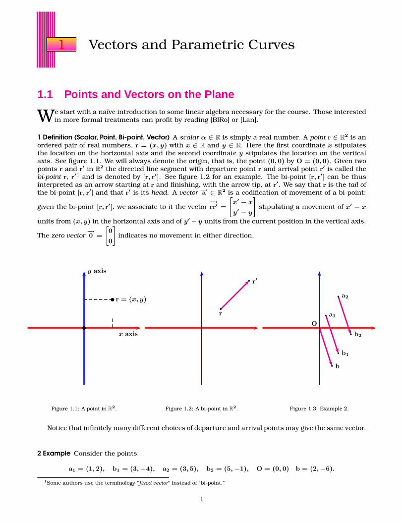
1 Definition (Scalar, Point, Bi-point, Vector) A scalar α ∈ R is simply a real number. A point r ∈ R2 is an
ordered pair of real numbers, r = (x, y) with x ∈ R and y ∈ R. Here the first coordinate x stipulatesthe location on the horizontal axis and the second coordinate y stipulates the location on the verticalaxis. See figure 1.1. We will always denote the origin, that is, the point (0, 0) by O = (0, 0). Given twopoints r and r′ in R
2 the directed line segment with departure point r and arrival point r′ is called thebi-point r, r′1 and is denoted by [r, r′]. See figure 1.2 for an example. The bi-point [r, r′] can be thusinterpreted as an arrow starting at r and finishing, with the arrow tip, at r′. We say that r is the tail ofthe bi-point [r, r′] and that r′ is its head. A vector −→a ∈ R
2 is a codification of movement of a bi-point:
given the bi-point [r, r′], we associate to it the vector−→rr′ =
"x′ − x
y′ − y
#stipulating a movement of x′ − x
units from (x, y) in the horizontal axis and of y′−y units from the current position in the vertical axis.
The zero vector−→0 =
"0
0
#indicates no movement in either direction.
x axis
y axis
b
b r = (x, y)
Figure 1.1: A point in R2.
b
b
r
r′
Figure 1.2: A bi-point in R2.
b
b
b
b
b
b
a1
b1
a2
b2
O
b
Figure 1.3: Example 2.
Notice that infinitely many different choices of departure and arrival points may give the same vector.
2 Example Consider the points
a1 = (1, 2), b1 = (3,−4), a2 = (3, 5), b2 = (5,−1), O = (0, 0) b = (2,−6).
1Some authors use the terminology “fixed vector” instead of “bi-point.”
1
Points and Vectors on the Plane
Though the bi-points [a1, b1], [a2, b2] and [O,b] are in different locations on the plane, they representthe same vector, as "
3− 1
−4− 2
#=
"5− 3
−1− 5
#=
"2− 0
−6− 0
#=
"2
−6
#.
The instructions given by the vector are all the same: start at the point, go two units right and six unitsdown. See figure 1.3.
In more technical language, a vector is an equivalence class of bi-points, that is, all bi-points thathave the same length, have the same direction, and point in the same sense are equivalent, and thename of this equivalence is a vector. As an simple example of an equivalence class, consider the set ofintegers Z. According to their remainder upon division by 3, each integer belongs to one of the threesets
3Z = . . . ,−6,−3, 0, 3, 6, . . ., 3Z+1 = . . . ,−5,−2, 1, 4, 7, . . ., 3Z+2 = . . . ,−4,−1, 2, 5, 8, . . ..
The equivalence class 3Z comprises the integers divisible by 3, and for example, −18 ∈ 3Z. Analogously,
in example 2, the bi-point [a1, b1] belongs to the equivalence class
"2
−6
#, that is, [a1, b1] ∈
"2
−6
#.
3 Definition The vector−→Oa that corresponds to the point a ∈ R
2 is called the position vector of the pointa.
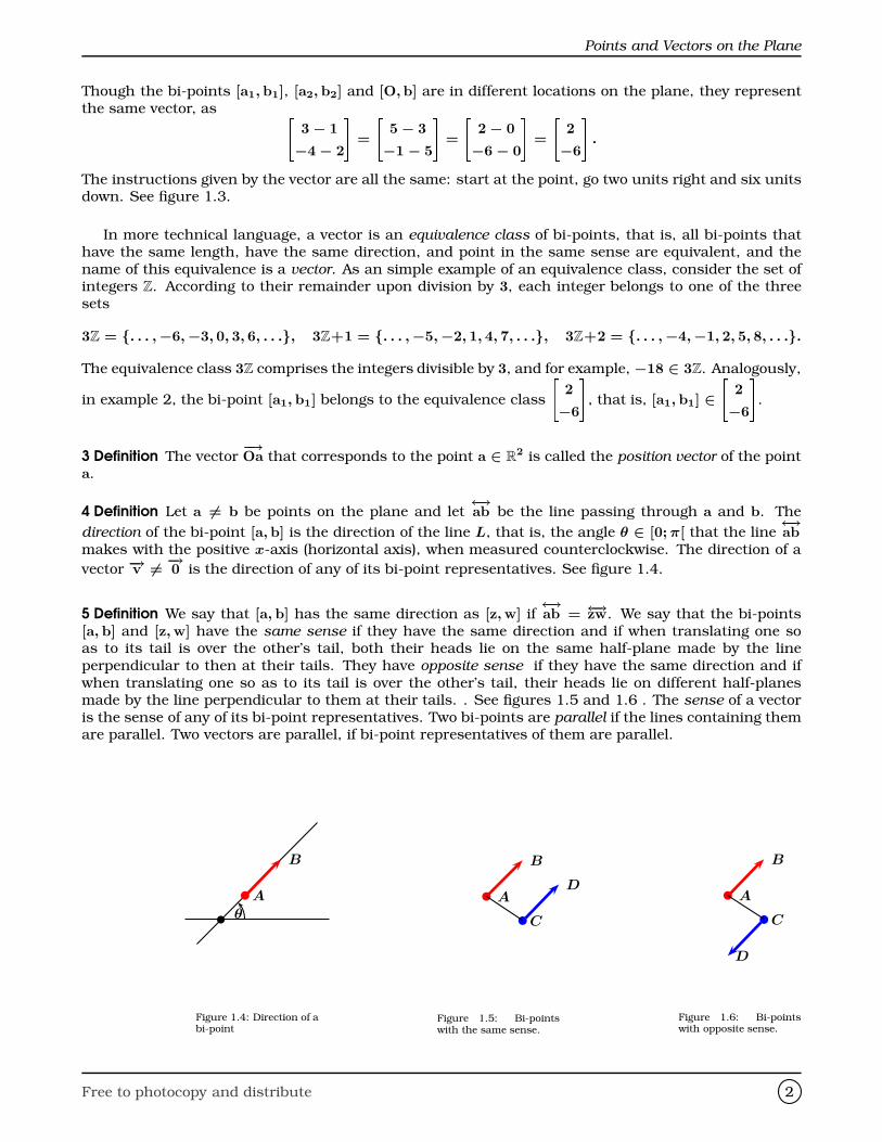
4 Definition Let a 6= b be points on the plane and let←→ab be the line passing through a and b. The
direction of the bi-point [a, b] is the direction of the line L, that is, the angle θ ∈ [0; π[ that the line←→ab
makes with the positive x-axis (horizontal axis), when measured counterclockwise. The direction of a
vector −→v 6= −→0 is the direction of any of its bi-point representatives. See figure 1.4.
5 Definition We say that [a, b] has the same direction as [z, w] if←→ab = ←→zw. We say that the bi-points
[a, b] and [z, w] have the same sense if they have the same direction and if when translating one soas to its tail is over the other’s tail, both their heads lie on the same half-plane made by the lineperpendicular to then at their tails. They have opposite sense if they have the same direction and ifwhen translating one so as to its tail is over the other’s tail, their heads lie on different half-planesmade by the line perpendicular to them at their tails. . See figures 1.5 and 1.6 . The sense of a vectoris the sense of any of its bi-point representatives. Two bi-points are parallel if the lines containing themare parallel. Two vectors are parallel, if bi-point representatives of them are parallel.
b θ
A
B
Figure 1.4: Direction of abi-point
A
B
C
D
Figure 1.5: Bi-pointswith the same sense.
A
B
C
D
Figure 1.6: Bi-pointswith opposite sense.
Free to photocopy and distribute 2
Chapter 1
Bi-point [b, a] has the opposite sense of [a, b] and so we write
[b, a] = −[a, b].
Similarly we write,−→ab = −−→ba.
6 Definition The Euclidean length or norm of bi-point [a, b] is simply the distance between a and b andit is denoted by
||[a, b]|| =È
(a1 − b1)2 + (a2 − b2)2.
A bi-point is said to have unit length if it has norm 1. The norm of a vector is the norm of any of itsbi-point representatives.
A vector is completely determined by three things: (i) its norm, (ii) its direction, and (iii) its sense. It
is clear that the norm of a vector satisfies the following properties:
1.−→a ≥ 0.
2.−→a = 0 ⇐⇒ −→a =
−→0 .
7 Example The vector −→v =
"1√2
#has norm
−→v = È12 + (
√2)2 =
√3.
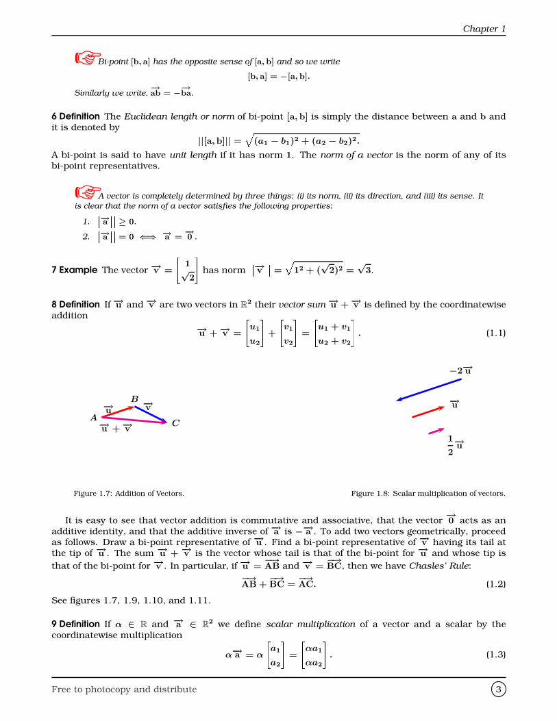
8 Definition If −→u and −→v are two vectors in R2 their vector sum −→u +−→v is defined by the coordinatewise
addition
−→u +−→v =
"u1
u2
#+
"v1
v2
#=
"u1 + v1
u2 + v2
#. (1.1)
A
B
C
−→v−→u−→u +−→v
Figure 1.7: Addition of Vectors.
−→u
1
2−→u
−2−→u
Figure 1.8: Scalar multiplication of vectors.
It is easy to see that vector addition is commutative and associative, that the vector−→0 acts as an
additive identity, and that the additive inverse of −→a is −−→a . To add two vectors geometrically, proceedas follows. Draw a bi-point representative of −→u . Find a bi-point representative of −→v having its tail atthe tip of −→u . The sum −→u + −→v is the vector whose tail is that of the bi-point for −→u and whose tip is
that of the bi-point for −→v . In particular, if −→u =−→AB and −→v =
−→BC, then we have Chasles’ Rule:
−→AB +
−→BC =
−→AC. (1.2)
See figures 1.7, 1.9, 1.10, and 1.11.
9 Definition If α ∈ R and −→a ∈ R2 we define scalar multiplication of a vector and a scalar by the
coordinatewise multiplication
α−→a = α
"a1
a2
#=
"αa1
αa2
#. (1.3)
Free to photocopy and distribute 3
Points and Vectors on the Plane
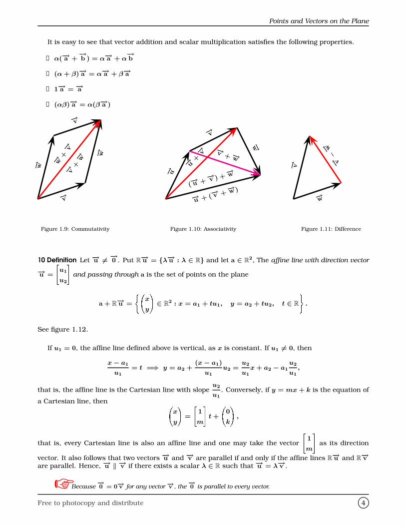
It is easy to see that vector addition and scalar multiplication satisfies the following properties.
➊ α(−→a +−→b ) = α−→a + α
−→b
➋ (α + β)−→a = α−→a + β−→a
➌ 1−→a = −→a
➍ (αβ)−→a = α(β−→a )
−→v
−→ w
−→ w
−→v
−→w+−→v
−→v+−→w
Figure 1.9: Commutativity
−→u
−→v
−→w
(−→u +
−→v ) +−→w
−→u + (−→v +
−→w)
−→v + −→w
−→u+−→v
Figure 1.10: Associativity
−→w
−→ v −→v−−→
w
Figure 1.11: Difference
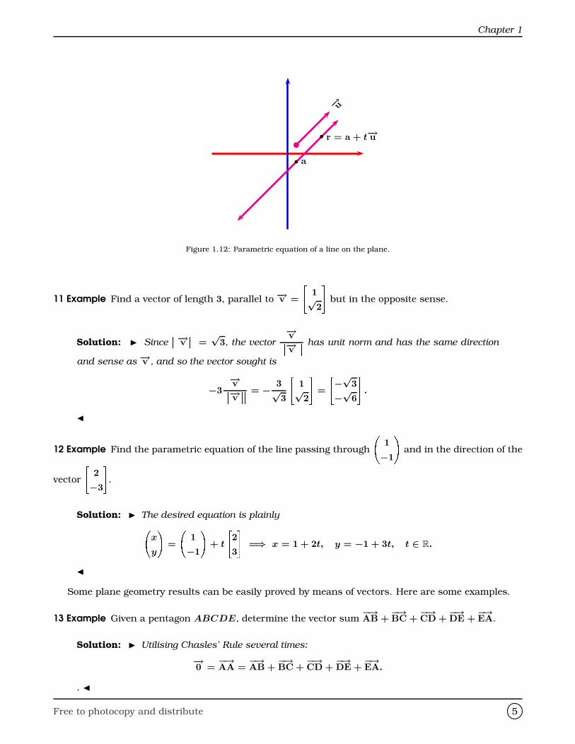
10 Definition Let −→u 6= −→0 . Put R−→u = λ−→u : λ ∈ R and let a ∈ R
2, The affine line with direction vector
−→u =
"u1
u2
#and passing through a is the set of points on the plane
a + R−→u =
( x
y
!∈ R
2 : x = a1 + tu1, y = a2 + tu2, t ∈ R
).
See figure 1.12.
If u1 = 0, the affine line defined above is vertical, as x is constant. If u1 6= 0, then
x− a1
u1
= t =⇒ y = a2 +(x− a1)
u1
u2 =u2
u1
x + a2 − a1
u2
u1
,
that is, the affine line is the Cartesian line with slopeu2
u1
. Conversely, if y = mx + k is the equation of
a Cartesian line, then x
y
!=
"1
m
#t +
0
k
!,
that is, every Cartesian line is also an affine line and one may take the vector
"1
m
#as its direction
vector. It also follows that two vectors −→u and −→v are parallel if and only if the affine lines R−→u and R
−→vare parallel. Hence, −→u ‖ −→v if there exists a scalar λ ∈ R such that −→u = λ−→v .
Because−→0 = 0−→v for any vector −→v , the
−→0 is parallel to every vector.
Free to photocopy and distribute 4
Chapter 1
−→u
b
b
a
r = a + t−→u
Figure 1.12: Parametric equation of a line on the plane.
11 Example Find a vector of length 3, parallel to −→v =
"1√2
#but in the opposite sense.
Solution: I Since−→v =
√3, the vector
−→v−→v has unit norm and has the same direction
and sense as −→v , and so the vector sought is
−3−→v−→v = − 3√
3
"1√2
#=
"−√
3
−√
6
#.
J
12 Example Find the parametric equation of the line passing through
1
−1
!and in the direction of the
vector
"2
−3
#.
Solution: I The desired equation is plainly x
y
!=
1
−1
!+ t
"2
3
#=⇒ x = 1 + 2t, y = −1 + 3t, t ∈ R.
J
Some plane geometry results can be easily proved by means of vectors. Here are some examples.
13 Example Given a pentagon ABCDE, determine the vector sum−→AB +
−→BC +
−→CD +
−→DE +
−→EA.
Solution: I Utilising Chasles’ Rule several times:
−→0 =
−→AA =
−→AB +
−→BC +
−→CD +
−→DE +
−→EA.
. J
Free to photocopy and distribute 5
Points and Vectors on the Plane
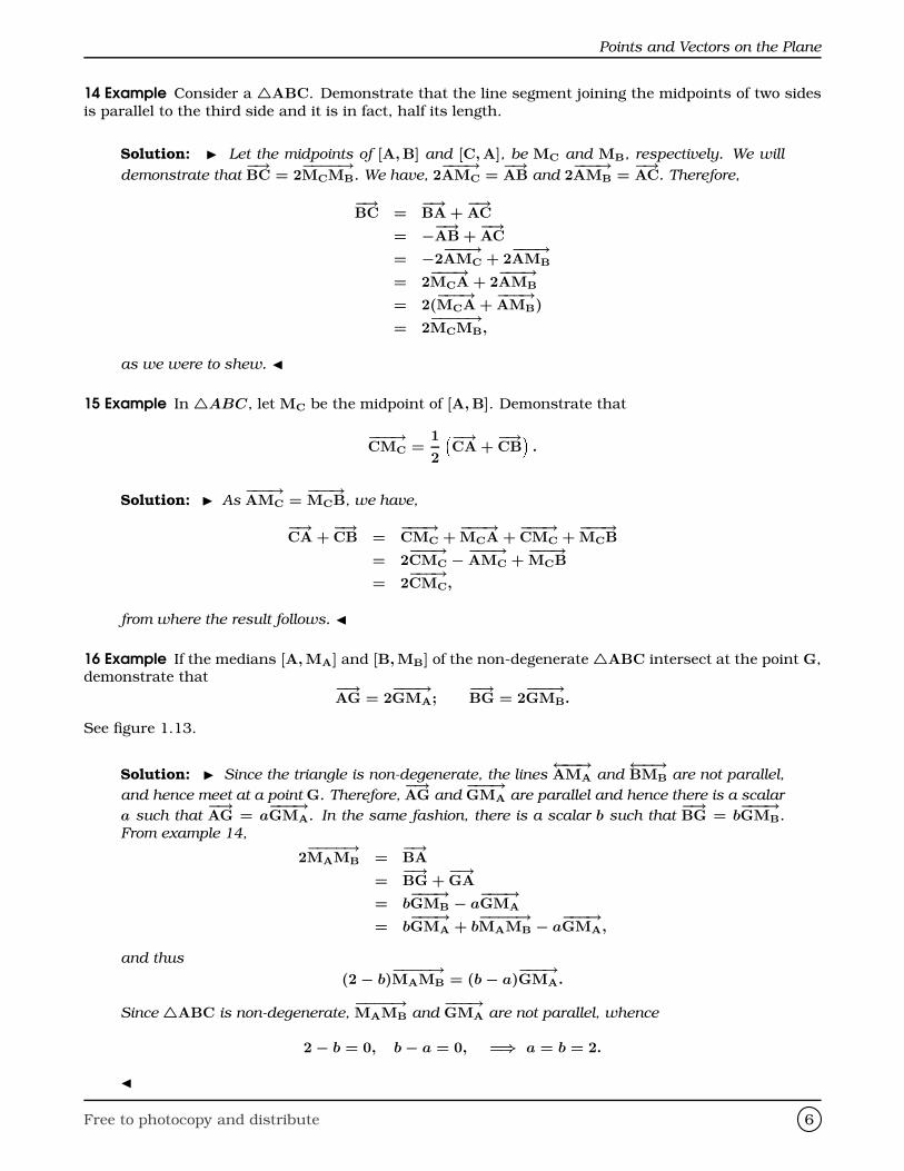
14 Example Consider a 4ABC. Demonstrate that the line segment joining the midpoints of two sidesis parallel to the third side and it is in fact, half its length.
Solution: I Let the midpoints of [A, B] and [C, A], be MC and MB, respectively. We will
demonstrate that−→BC = 2
−−−−→MCMB. We have, 2
−−−→AMC =
−→AB and 2
−−−→AMB =
−→AC. Therefore,
−→BC =
−→BA +
−→AC
= −−→AB +−→AC
= −2−−−→AMC + 2
−−−→AMB
= 2−−−→MCA + 2
−−−→AMB
= 2(−−−→MCA +
−−−→AMB)
= 2−−−−→MCMB,
as we were to shew. J
15 Example In 4ABC, let MC be the midpoint of [A, B]. Demonstrate that
−−−→CMC =
1
2
−→CA +
−→CB
.
Solution: I As−−−→AMC =
−−−→MCB, we have,
−→CA +
−→CB =
−−−→CMC +
−−−→MCA +
−−−→CMC +
−−−→MCB
= 2−−−→CMC −
−−−→AMC +
−−−→MCB
= 2−−−→CMC,
from where the result follows. J
16 Example If the medians [A, MA] and [B, MB] of the non-degenerate4ABC intersect at the point G,demonstrate that −→
AG = 2−−−→GMA;
−→BG = 2
−−−→GMB.
See figure 1.13.
Solution: I Since the triangle is non-degenerate, the lines←−−→AMA and
←−→BMB are not parallel,
and hence meet at a point G. Therefore,−→AG and
−−−→GMA are parallel and hence there is a scalar
a such that−→AG = a
−−−→GMA. In the same fashion, there is a scalar b such that
−→BG = b
−−−→GMB.
From example 14,
2−−−−→MAMB =
−→BA
=−→BG +
−→GA
= b−−−→GMB − a
−−−→GMA
= b−−−→GMA + b
−−−−→MAMB − a
−−−→GMA,
and thus
(2− b)−−−−→MAMB = (b− a)
−−−→GMA.
Since4ABC is non-degenerate,−−−−→MAMB and
−−−→GMA are not parallel, whence
2− b = 0, b− a = 0, =⇒ a = b = 2.
J
Free to photocopy and distribute 6
Chapter 1
b
Ab
B
bC
b
MC
bMB bMA
b
G
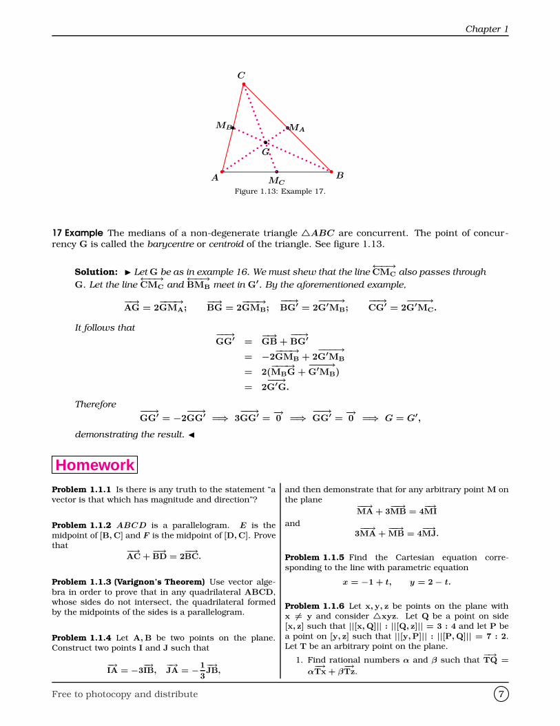
Figure 1.13: Example 17.
17 Example The medians of a non-degenerate triangle 4ABC are concurrent. The point of concur-rency G is called the barycentre or centroid of the triangle. See figure 1.13.
Solution: I Let G be as in example 16. We must shew that the line←−→CMC also passes through
G. Let the line←−→CMC and
←−→BMB meet in G′. By the aforementioned example,
−→AG = 2
−−−→GMA;
−→BG = 2
−−−→GMB;
−−→BG′ = 2
−−−→G′MB;
−−→CG′ = 2
−−−→G′MC.
It follows that −−→GG′ =
−→GB +
−−→BG′
= −2−−−→GMB + 2
−−−→G′MB
= 2(−−−→MBG +
−−−→G′MB)
= 2−−→G′G.
Therefore −−→GG′ = −2
−−→GG′ =⇒ 3
−−→GG′ =
−→0 =⇒
−−→GG′ =
−→0 =⇒ G = G′,
demonstrating the result. J
HomeworkProblem 1.1.1 Is there is any truth to the statement “a
vector is that which has magnitude and direction”?
Problem 1.1.2 ABCD is a parallelogram. E is the
midpoint of [B, C] and F is the midpoint of [D, C]. Provethat −→
AC +−→BD = 2
−→BC.
Problem 1.1.3 (Varignon’s Theorem) Use vector alge-
bra in order to prove that in any quadrilateral ABCD,whose sides do not intersect, the quadrilateral formedby the midpoints of the sides is a parallelogram.
Problem 1.1.4 Let A, B be two points on the plane.Construct two points I and J such that
−→IA = −3
−→IB,
−→JA = −1
3
−→JB,
and then demonstrate that for any arbitrary point M on
the plane −−→MA + 3
−−→MB = 4
−→MI
and3−−→MA +
−−→MB = 4
−→MJ.
Problem 1.1.5 Find the Cartesian equation corre-
sponding to the line with parametric equation
x = −1 + t, y = 2− t.
Problem 1.1.6 Let x, y, z be points on the plane withx 6= y and consider 4xyz. Let Q be a point on side[x, z] such that ||[x, Q]|| : ||[Q, z]|| = 3 : 4 and let P be
a point on [y, z] such that ||[y, P]|| : ||[P, Q]|| = 7 : 2.Let T be an arbitrary point on the plane.
1. Find rational numbers α and β such that−→TQ =
α−→Tx + β
−→Tz.
Free to photocopy and distribute 7
Scalar Product on the Plane
2. Find rational numbers l, m, n such that−→TP =
l−→Tx + m
−→Ty + n
−→Tz.
Problem 1.1.7 Let x, y, z be points on the plane with
x 6= y. Demonstrate that
1. The point a belongs to the line ←→xy if and only ifthere exists scalars α, β with α + β = 1 such that
−→za = α−→zx + β−→zy.
2. The point a belongs to the line segment [x; y] if
and only if there exists scalars α ≥ 0, β ≥ 0 withα + β = 1 such that
−→za = α−→zx + β−→zy.
3. The point a belongs to the interior of the tri-
angle 4xyz if and only if there exists scalarsα > 0, β > 0 with α + β < 1 such that
−→za = α−→zx + β−→zy.
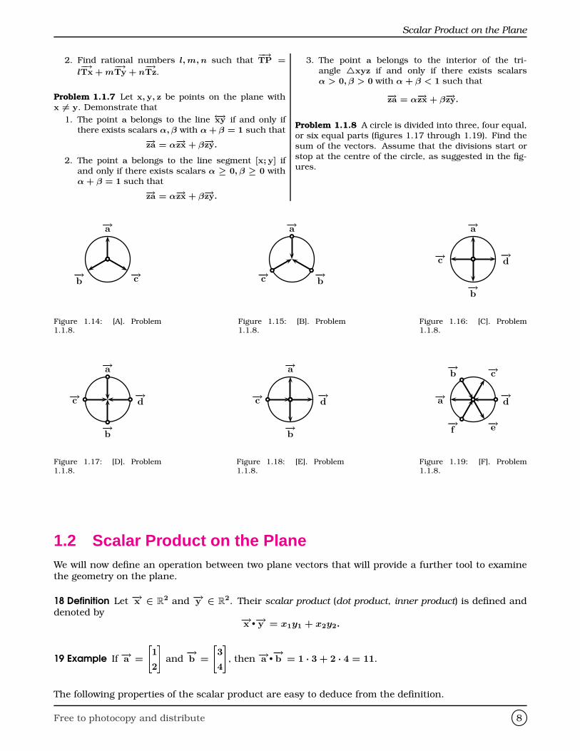
Problem 1.1.8 A circle is divided into three, four equal,or six equal parts (figures 1.17 through 1.19). Find the
sum of the vectors. Assume that the divisions start orstop at the centre of the circle, as suggested in the fig-ures.
−→a
−→b
−→c
Figure 1.14: [A]. Problem1.1.8.
−→a
−→b
−→c
Figure 1.15: [B]. Problem1.1.8.
−→a
−→b
−→c −→d
Figure 1.16: [C]. Problem1.1.8.
−→a
−→b
−→c −→d
Figure 1.17: [D]. Problem1.1.8.
−→a
−→b
−→c −→d
Figure 1.18: [E]. Problem1.1.8.
−→a −→d
−→b −→c
−→f
−→e
Figure 1.19: [F]. Problem1.1.8.
1.2 Scalar Product on the PlaneWe will now define an operation between two plane vectors that will provide a further tool to examinethe geometry on the plane.
18 Definition Let −→x ∈ R2 and −→y ∈ R
2. Their scalar product (dot product, inner product) is defined anddenoted by −→x •−→y = x1y1 + x2y2.
19 Example If −→a =
"1
2
#and−→b =
"3
4
#, then −→a •
−→b = 1 · 3 + 2 · 4 = 11.
The following properties of the scalar product are easy to deduce from the definition.
Free to photocopy and distribute 8
Chapter 1
SP1 Bilinearity(−→x +−→y )•−→z = −→x •−→z +−→y •−→z , −→x •(−→y +−→z ) = −→x •−→y +−→x •−→z (1.4)
SP2 Scalar Homogeneity(α−→x )•−→y = −→x •(α−→y ) = α(−→x •−→y ), α ∈ R. (1.5)
SP3 Commutativity −→x •−→y = −→y •−→x (1.6)
SP4 −→x •−→x ≥ 0 (1.7)
SP5 −→x •−→x = 0 ⇐⇒ −→x =−→0 (1.8)
SP6 −→x = p−→x •−→x (1.9)
−→a−→b −−→a
−→b
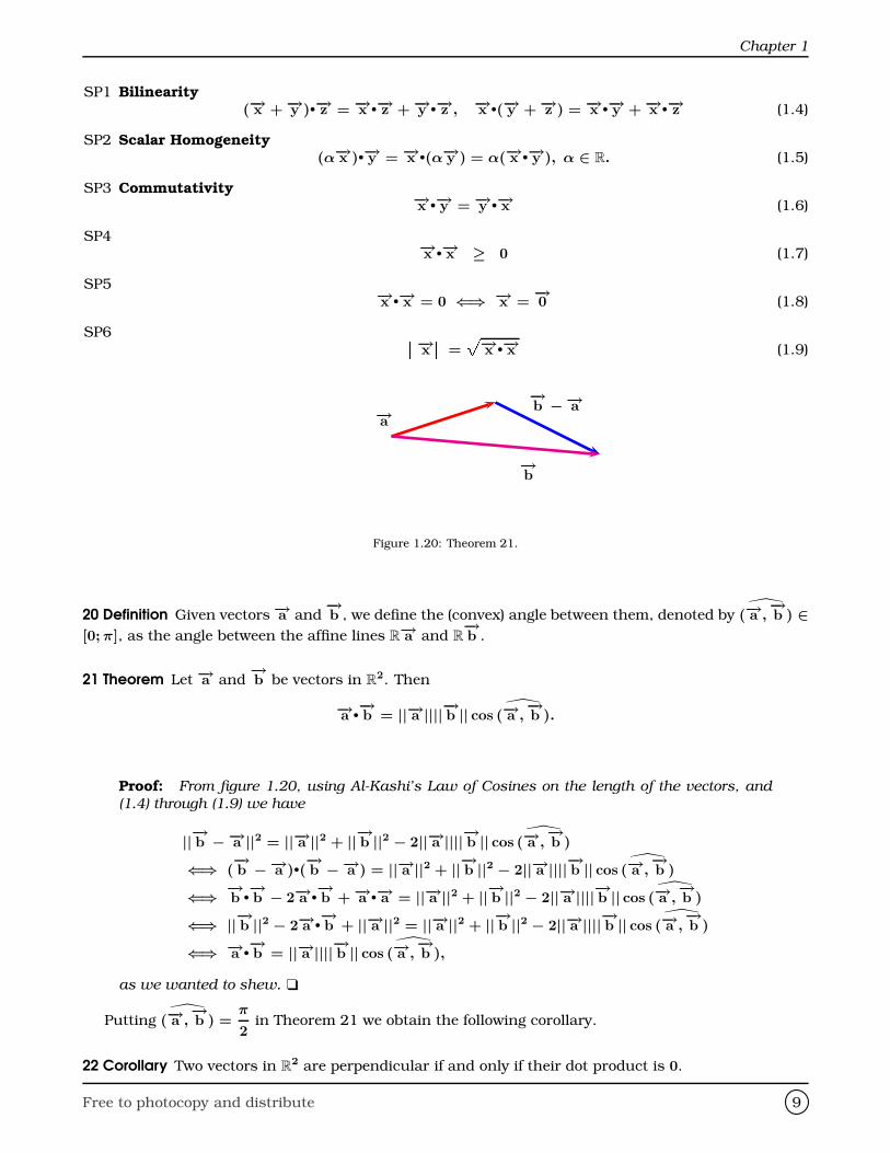
Figure 1.20: Theorem 21.
20 Definition Given vectors −→a and−→b , we define the (convex) angle between them, denoted by
(−→a ,−→b ) ∈
[0; π], as the angle between the affine lines R−→a and R
−→b .
21 Theorem Let −→a and−→b be vectors in R
2. Then
−→a •−→b = ||−→a ||||−→b || cos
(−→a ,−→b ).
Proof: From figure 1.20, using Al-Kashi’s Law of Cosines on the length of the vectors, and
(1.4) through (1.9) we have
||−→b −−→a ||2 = ||−→a ||2 + ||−→b ||2 − 2||−→a ||||−→b || cos
(−→a ,−→b )
⇐⇒ (−→b −−→a )•(
−→b −−→a ) = ||−→a ||2 + ||−→b ||2 − 2||−→a ||||−→b || cos
(−→a ,−→b )
⇐⇒ −→b •−→b − 2−→a •
−→b +−→a •−→a = ||−→a ||2 + ||−→b ||2 − 2||−→a ||||−→b || cos
(−→a ,−→b )
⇐⇒ ||−→b ||2 − 2−→a •−→b + ||−→a ||2 = ||−→a ||2 + ||−→b ||2 − 2||−→a ||||−→b || cos
(−→a ,−→b )
⇐⇒ −→a •−→b = ||−→a ||||−→b || cos
(−→a ,−→b ),
as we wanted to shew.
Putting
(−→a ,−→b ) =
π
2in Theorem 21 we obtain the following corollary.
22 Corollary Two vectors in R2 are perpendicular if and only if their dot product is 0.
Free to photocopy and distribute 9
Scalar Product on the Plane
It follows that the vector−→0 is simultaneously parallel and perpendicular to any vector!
23 Definition Two vectors are said to be orthogonal if they are perpendicular. If −→a is orthogonal to−→b ,
we write −→a ⊥ −→b .
24 Definition If −→a ⊥ −→b and−→a = −→b = 1 we say that −→a and
−→b are orthonormal.
Since | cos θ| ≤ 1 we also have
25 Corollary (Cauchy-Bunyakovsky-Schwarz Inequality)−→a •−→b ≤ −→a −→b .
Equality occurs if and only if −→a ‖ −→b .
If −→a =
"a1
a2
#and−→b =
"b1
b2
#, the CBS Inequality takes the form
|a1b1 + a2b2| ≤ (a21 + a2
2)1/2(b2
1 + b22)
1/2. (1.10)
26 Example Let a, b be positive real numbers. Minimise a2 + b2 subject to the constraint a + b = 1.
Solution: I By the CBS Inequality,
1 = |a · 1 + b · 1| ≤ (a2 + b2)1/2(12 + 12)1/2 =⇒ a2 + b2 ≥ 1
2.
Equality occurs if and only if
"a
b
#= λ
"1
1
#. In such case, a = b = λ, and so equality is achieved
for a = b =1
2. J
27 Corollary (Triangle Inequality) −→a +−→b ≤ −→a + −→b .
Proof:||−→a +
−→b ||2 = (−→a +
−→b )•(−→a +
−→b )
= −→a •−→a + 2−→a •−→b +
−→b •−→b
≤ ||−→a ||2 + 2||−→a ||||−→b ||+ ||−→b ||2
= (||−→a ||+ ||−→b ||)2,
from where the desired result follows.
28 Example Let x, y, z be positive real numbers. Prove that√
2(x + y + z) ≤È
x2 + y2 +È
y2 + z2 +p
z2 + x2.
Solution: I Put −→a =
"x
y
#,−→b =
"y
z
#, −→c =
"z
x
#. Then−→a +
−→b +−→c
= "x + y + z
x + y + z
# = √2(x + y + z).
Free to photocopy and distribute 10
Chapter 1
Also, −→a + −→b + −→c = Èx2 + y2 +
Èy2 + z2 +
pz2 + x2,
and the assertion follows by the triangle inequality−→a +−→b +−→c
≤ −→a + −→b + −→c .J
We now use vectors to prove a classical theorem of Euclidean geometry.
29 Definition Let A and B be points on the plane and let −→u be a unit vector. If−→AB = λ−→u , then λ is
the directed distance or algebraic measure of the line segment [AB] with respect to the vector −→u . Wewill denote this distance by AB−→u , or more routinely, if the vector −→u is patent, by AB. Observe thatAB = −BA.
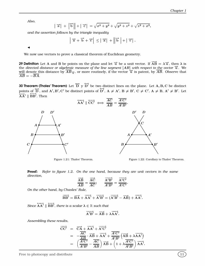
30 Theorem (Thales’ Theorem) Let←→D y
←→D′ be two distinct lines on the plane. Let A, B, C be distinct
points of←→D , and A′, B′, C′ be distinct points of
←→D′ , A 6= A′, B 6= B′, C 6= C′, A 6= B, A′ 6= B′. Let
←→AA′ ‖
←→BB′. Then
←−→AA′ ‖
←→CC′ ⇐⇒ AC
AB=
A′C′
A′B′ .
D D′
bA b A′
bB b B′
bC b C′
Figure 1.21: Thales’ Theorem.
DD′
b C
bA b A′
bB b B′
Figure 1.22: Corollary to Thales’ Theorem.
Proof: Refer to figure 1.2. On the one hand, because they are unit vectors in the same
direction, −→AB
AB=
−→AC
AC;
−−→A′B′
A′B′ =
−−→A′C′
A′C′ .
On the other hand, by Chasles’ Rule,
−−→BB′ =
−→BA +
−−→AA′ +
−−→A′B′ = (
−−→A′B′ −−→AB) +
−−→AA′.
Since←−→AA′ ‖
←→BB′, there is a scalar λ ∈ R such that
−−→A′B′ =
−→AB + λ
−−→AA′.
Assembling these results,
−−→CC′ =
−→CA +
−−→AA′ +
−−→A′C′
= −AC
AB· −→AB +
−−→AA′ +
A′C′
A′B′
−→AB + λ
−−→AA′
=
A′C′
A′B′ −AC
AB
−→AB +
1 + λ
A′C′
A′B′
−−→AA′.
Free to photocopy and distribute 11
Linear Independence
As the line←−→AA′ is not parallel to the line
←→AB, the equality above reveals that
←−→AA′ ‖
←→CC′ ⇐⇒ AC
AB− A′C′
A′B′ = 0,
proving the theorem.
From the preceding theorem, we immediately gather the following corollary. (See figure 1.2.)
31 Corollary Let←→D and
←→D′ are distinct lines, intersecting in the unique point C. Let A, B, be points
on line←→D , and A′, B′, points on line
←→D′ . Then
←−→AA′ ‖
←→BB′ ⇐⇒ CB
CA=
CB′
CA′ .
1.3 Linear Independence
Consider now two arbitrary vectors in R2, −→x and −→y , say. Under which conditions can we write an
arbitrary vector −→v on the plane as a linear combination of −→x and −→y , that is, when can we findscalars a, b such that −→v = a−→x + b−→y ?
The answer can be promptly obtained algebraically. Operating formally,
−→v = a−→x + b−→y ⇐⇒ v1 = ax1 + by1, v2 = ax2 + by2
⇐⇒ a =v1y2 − v2y1
x1y2 − x2y1
, b =x1v2 − x2v1
x1y2 − x2y1
.
The above expressions for a and b make sense only if x1y2 6= x2y1. But, what does it mean x1y2 =
x2y1? If none of these are zero thenx1
y1
=x2
y2
= λ, say, and to"x1
x2
#= λ
"y1
y2
#⇐⇒ −→x ‖ −→y .
If x1 = 0, then either x2 = 0 or y1 = 0. In the first case, −→x =−→0 , and a fortiori −→x ‖ −→y , since all
vectors are parallel to the zero vector. In the second case we have
−→x = x2−→j , −→y = y2
−→j ,
and so both vectors are parallel to−→j and hence −→x ‖ −→y . We have demonstrated the following theorem.
32 Theorem Given two vectors in R2, −→x and −→y , an arbitrary vector −→v can be written as the linear
combination −→v = a−→x + b−→y , a ∈ R, b ∈ R
if and only if −→x is not parallel to −→y . In this last case we say that −→x is linearly independent from vector−→y . If two vectors are not linearly independent, then we say that they are linearly dependent.
33 Example The vectors
"1
0
#and
"1
1
#are clearly linearly independent, since one is not a scalar multiple
of the other. Given an arbitrary vector
"a
b
#we can express it as a linear combination of these vectors
as follows: "a
b
#= (a− b)
"1
0
#+ b
"1
1
#.
Free to photocopy and distribute 12
Chapter 1
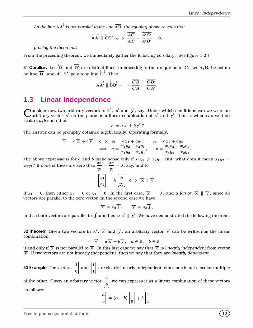
Consider now two linearly independent vectors −→x and −→y . For a ∈ [0; 1], a−→x is parallel to −→x andtraverses the whole length of −→x : from its tip (when a = 1) to its tail (when a = 0). In the same manner,for b ∈ [0; 1], b−→y is parallel to−→y and traverses the whole length of −→y . The linear combination a−→x +b−→yis also a vector on the plane.
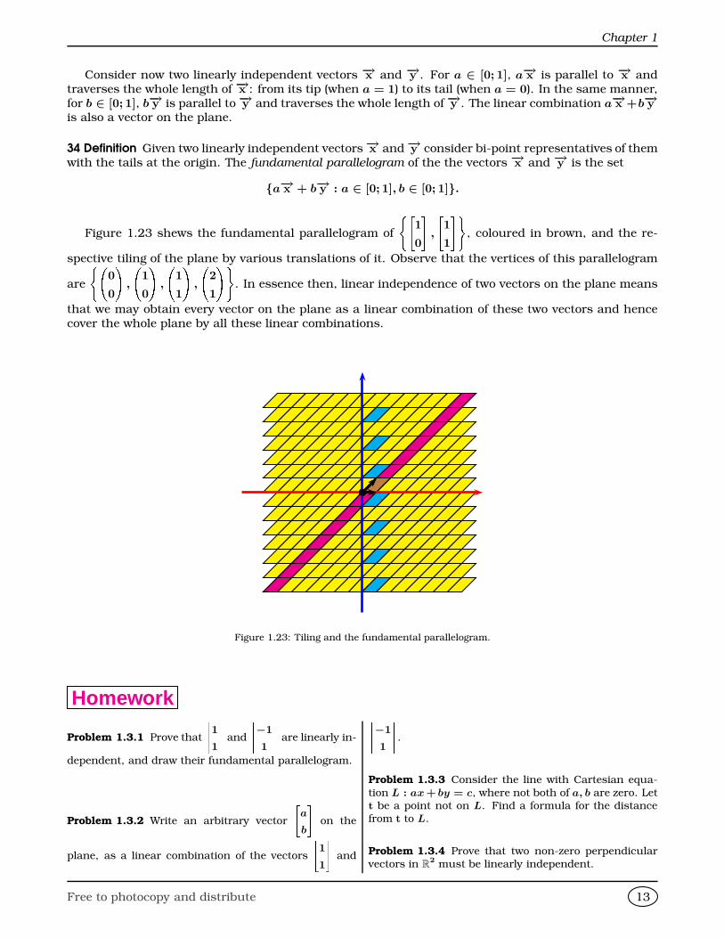
34 Definition Given two linearly independent vectors−→x and−→y consider bi-point representatives of themwith the tails at the origin. The fundamental parallelogram of the the vectors −→x and −→y is the set
a−→x + b−→y : a ∈ [0; 1], b ∈ [0; 1].
Figure 1.23 shews the fundamental parallelogram of
("1
0
#,
"1
1
#), coloured in brown, and the re-
spective tiling of the plane by various translations of it. Observe that the vertices of this parallelogram
are
( 0
0
!,
1
0
!,
1
1
!,
2
1
!). In essence then, linear independence of two vectors on the plane means
that we may obtain every vector on the plane as a linear combination of these two vectors and hencecover the whole plane by all these linear combinations.
Figure 1.23: Tiling and the fundamental parallelogram.
Homework
Problem 1.3.1 Prove that
1
1
and
−1
1
are linearly in-
dependent, and draw their fundamental parallelogram.
Problem 1.3.2 Write an arbitrary vector
a
b
on the
plane, as a linear combination of the vectors
1
1
and
−1
1
.
Problem 1.3.3 Consider the line with Cartesian equa-
tion L : ax + by = c, where not both of a, b are zero. Lett be a point not on L. Find a formula for the distancefrom t to L.
Problem 1.3.4 Prove that two non-zero perpendicularvectors in R
2 must be linearly independent.
Free to photocopy and distribute 13
Geometric Transformations in two dimensions
1.4 Geometric Transformations in two dimensions
We now are interested in the following fundamental functions of sets (figures) on the plane: transla-tions, scalings (stretching or shrinking) reflexions about the axes, and rotations about the origin.
It will turn out that a handy tool for investigating all of these (with the exception of translations), willbe certain construct called matrices which we will study in the next section.
First observe what is meant by a function F : R2 → R
2. This means that the input of the function isa point of the plane, and the output is also a point on the plane.
A rather uninteresting example, but nevertheless an important one is the following.
35 Example The function I : R2 → R
2, I(x) = x is called the identity transformation. Observe that theidentity transformation leaves a point untouched.
We start with the simplest of these functions.
36 Definition A function T−→v : R2 → R
2 is said to be a translation if it is of the form T−→v (x) = x + −→v ,where −→v is a fixed vector on the plane.
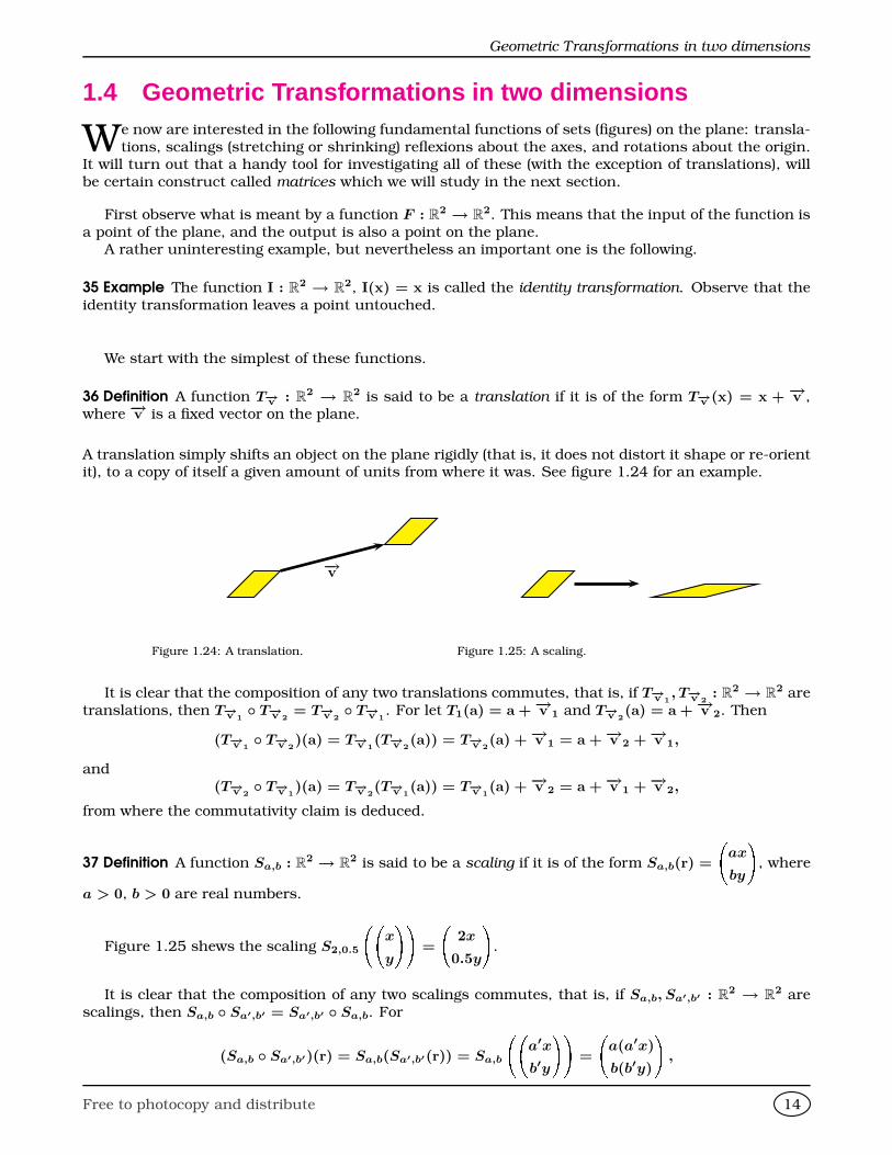
A translation simply shifts an object on the plane rigidly (that is, it does not distort it shape or re-orientit), to a copy of itself a given amount of units from where it was. See figure 1.24 for an example.
−→v
Figure 1.24: A translation. Figure 1.25: A scaling.
It is clear that the composition of any two translations commutes, that is, if T−→v 1, T−→v 2
: R2 → R
2 aretranslations, then T−→v 1
T−→v 2= T−→v 2
T−→v 1. For let T1(a) = a +−→v 1 and T−→v 2
(a) = a +−→v 2. Then
(T−→v 1 T−→v 2
)(a) = T−→v 1(T−→v 2
(a)) = T−→v 2(a) +−→v 1 = a +−→v 2 +−→v 1,
and(T−→v 2
T−→v 1)(a) = T−→v 2
(T−→v 1(a)) = T−→v 1
(a) +−→v 2 = a +−→v 1 +−→v 2,
from where the commutativity claim is deduced.
37 Definition A function Sa,b : R2 → R
2 is said to be a scaling if it is of the form Sa,b(r) =
ax
by
!, where
a > 0, b > 0 are real numbers.
Figure 1.25 shews the scaling S2,0.5
x
y
!!=
2x
0.5y
!.
It is clear that the composition of any two scalings commutes, that is, if Sa,b, Sa′,b′ : R2 → R
2 arescalings, then Sa,b Sa′,b′ = Sa′,b′ Sa,b. For
(Sa,b Sa′,b′)(r) = Sa,b(Sa′,b′(r)) = Sa,b
a′x
b′y
!!=
a(a′x)
b(b′y)
!,
Free to photocopy and distribute 14
Chapter 1
and
(Sa′,b′ Sa,b)(r) = Sa′,b′(Sa,b(r)) = Sa′,b′
ax
by
!!=
a′(ax)
b′(by)
!,
from where the commutativity claim is deduced.
Translations and scalings do not necessarily commute, however. For consider the translation
T−→i(a) = a +
−→i and the scaling S2,1(a) =
2a1
a2
!. Then
(T−→i S2,1)
−1
0
!!= T−→
i
S
−1
0
!!!= T−→
i
−2
0
!!=
−1
0
!,
but
(S2,1 T−→i)
−1
0
!!= S2,1
T−→
i
−1
0
!!!= S2,1
0
0
!!=
0
0
!.
x axis
y axis
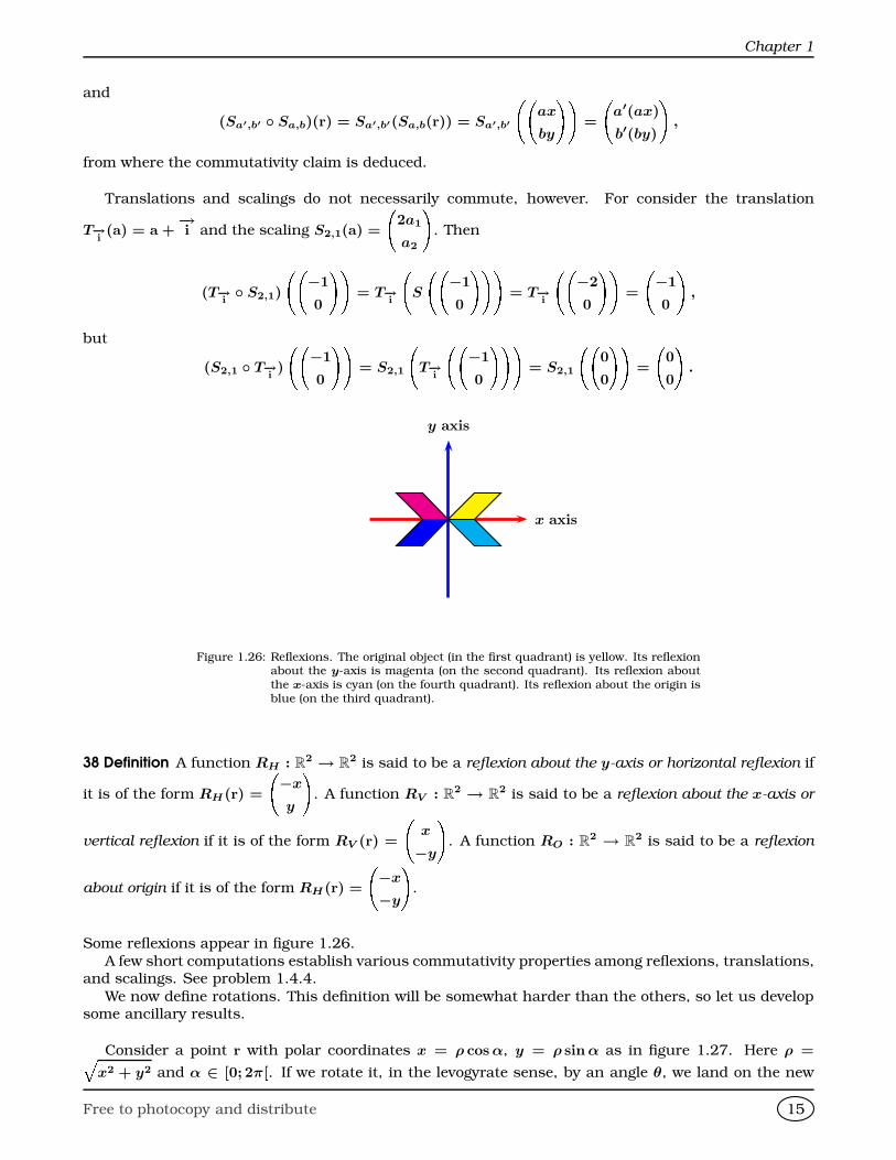
Figure 1.26: Reflexions. The original object (in the first quadrant) is yellow. Its reflexionabout the y-axis is magenta (on the second quadrant). Its reflexion aboutthe x-axis is cyan (on the fourth quadrant). Its reflexion about the origin isblue (on the third quadrant).
38 Definition A function RH : R2 → R
2 is said to be a reflexion about the y-axis or horizontal reflexion if
it is of the form RH(r) =
−x
y
!. A function RV : R
2 → R2 is said to be a reflexion about the x-axis or
vertical reflexion if it is of the form RV (r) =
x
−y
!. A function RO : R
2 → R2 is said to be a reflexion
about origin if it is of the form RH(r) =
−x
−y
!.
Some reflexions appear in figure 1.26.A few short computations establish various commutativity properties among reflexions, translations,
and scalings. See problem 1.4.4.
We now define rotations. This definition will be somewhat harder than the others, so let us developsome ancillary results.
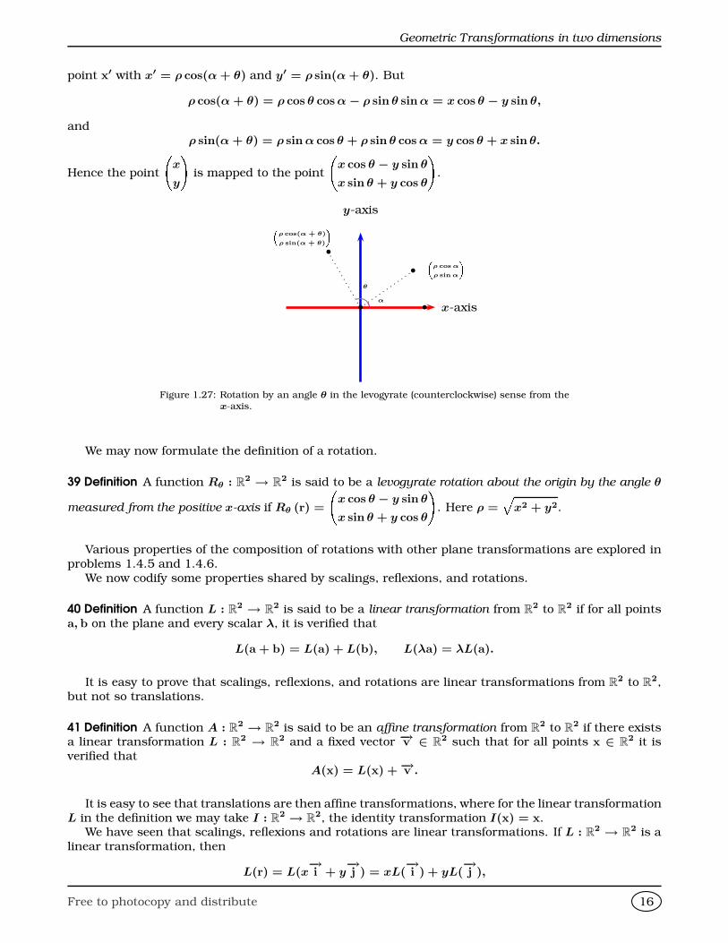
Consider a point r with polar coordinates x = ρ cos α, y = ρ sin α as in figure 1.27. Here ρ =Èx2 + y2 and α ∈ [0; 2π[. If we rotate it, in the levogyrate sense, by an angle θ, we land on the new
Free to photocopy and distribute 15
Geometric Transformations in two dimensions
point x′ with x′ = ρ cos(α + θ) and y′ = ρ sin(α + θ). But
ρ cos(α + θ) = ρ cos θ cos α− ρ sin θ sin α = x cos θ − y sin θ,
andρ sin(α + θ) = ρ sin α cos θ + ρ sin θ cos α = y cos θ + x sin θ.
Hence the point
x
y
!is mapped to the point
x cos θ − y sin θ
x sin θ + y cos θ
!.
x-axis
y-axis
b
b
b
bα
θ
ρ cos α
ρ sin α
ρ cos(α + θ)
ρ sin(α + θ)
Figure 1.27: Rotation by an angle θ in the levogyrate (counterclockwise) sense from the
x-axis.
We may now formulate the definition of a rotation.
39 Definition A function Rθ : R2 → R
2 is said to be a levogyrate rotation about the origin by the angle θ
measured from the positive x-axis if Rθ (r) =
x cos θ − y sin θ
x sin θ + y cos θ
!. Here ρ =
Èx2 + y2.
Various properties of the composition of rotations with other plane transformations are explored inproblems 1.4.5 and 1.4.6.
We now codify some properties shared by scalings, reflexions, and rotations.
40 Definition A function L : R2 → R
2 is said to be a linear transformation from R2 to R
2 if for all pointsa, b on the plane and every scalar λ, it is verified that
L(a + b) = L(a) + L(b), L(λa) = λL(a).
It is easy to prove that scalings, reflexions, and rotations are linear transformations from R2 to R
2,but not so translations.
41 Definition A function A : R2 → R
2 is said to be an affine transformation from R2 to R
2 if there existsa linear transformation L : R
2 → R2 and a fixed vector −→v ∈ R
2 such that for all points x ∈ R2 it is
verified thatA(x) = L(x) +−→v .
It is easy to see that translations are then affine transformations, where for the linear transformationL in the definition we may take I : R
2 → R2, the identity transformation I(x) = x.
We have seen that scalings, reflexions and rotations are linear transformations. If L : R2 → R
2 is alinear transformation, then
L(r) = L(x−→i + y
−→j ) = xL(
−→i ) + yL(
−→j ),
Free to photocopy and distribute 16
Chapter 1
and thus a linear transformation from R2 to R
2 is solely determined by the values L(−→i ) and L(
−→j ). We
will now introduce a way to codify these values.
42 Definition Let L : R2 → R
2 be a linear transformation. The matrix AL associated to L is the 2× 2, (2
rows, 2 columns) array whose columns are (in this order) L
1
0
!!and L
0
1
!!.
43 Example (Scaling Matrices) Let a > 0, b > 0 be a real numbers. The matrix of the scaling transfor-
mation Sa,b is
"a 0
0 b
#. For
Sa,b
1
0
!!=
a · 1b · 0
!=
a
0
!and
Sa,b
0
1
!!=
0 · 1b · 1
!=
0
b
!.
44 Example (Reflexion Matrices) It is easy to verify that the matrix for the transformation RH is
"−1 0
0 1
#,
that the matrix for the transformation RV is
"1 0
0 −1
#, and the matrix for the transformation RO is"
−1 0
0 −1
#.
45 Example (Rotating Matrices) It is easy to verify that the matrix for a rotation Rθ is
"cos θ − sin θ
sin θ cos θ
#.
46 Example (Identity Matrix) The matrix for the identity linear transformation Id : R2 → R
2, Id(x) = x
is I2 =
"1 0
0 1
#.
47 Example (Zero Matrix) The matrix for the null linear transformation N : R2 → R
2, N(x) = O is
02 =
"0 0
0 0
#.
From problem 1.4.7 we know that the composition of two linear transformations is also linear. Weare now interested in how to codify the matrix of a composition of linear transformations L1 L1 interms of their individual matrices.
48 Theorem Let L : R2 → R
2 have the matrix representation AL =
"a b
c d
#and let L′ : R
2 → R2 have
the matrix representation AL′ =
"r s
t u
#. Then the composition L L′ has matrix representation"
ar + bt as + bu
cr + dt cs + du
#.
Free to photocopy and distribute 17
Geometric Transformations in two dimensions
Proof: We need to find (L L′)
1
0
!!and (L L′)
0
1
!!.
We have
(LL′)
1
0
!!= L
L′
1
0
!!!= L
r
t
!!= rL(
−→i )+tL(
−→j ) = r
a
c
!+t
b
d
!=
ar + bt
cr + dt
!,
and
(LL′)
0
1
!!= L
L′
0
1
!!!= L
s
u
!!= sL(
−→i )+uL(
−→j ) = s
a
c
!+u
b
d
!=
as + bu
cs + du
!,
whence we conclude that the matrix of L L′ is
"ar + bt as + bu
cr + dt cs + du
#, as we wanted to shew.
The above motivates the following definition.
49 Definition Let A =
"a b
c d
#and B =
"r s
t u
#be two 2× 2 matrices, and λ ∈ R be a scalar. We define
matrix addition as
A + B =
"a b
c d
#+
"r s
t u
#=
"a + r b + s
c + t d + u
#.
We define matrix multiplication as
AB =
"a b
c d
# "r s
t u
#=
"ar + bt as + bu
cr + dt cs + du
#.
We define scalar multiplication of a matrix as
λA = λ
"a b
c d
#=
"λa λb
λc λd
#.
Since the composition of functions is not necessarily commutative, neither is matrix multiplication.
Since the composition of functions is associative, so is matrix multiplication.
50 Example Let
M =
"1 −1
0 1
#, N =
"1 2
−2 1
#.
Then
M + N =
"2 1
−2 2
#, 2M =
"2 −2
0 2
#, MN =
"3 1
−2 1
#.
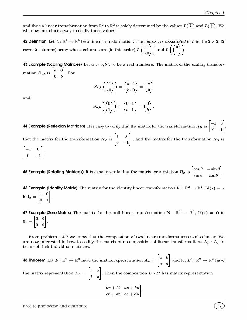
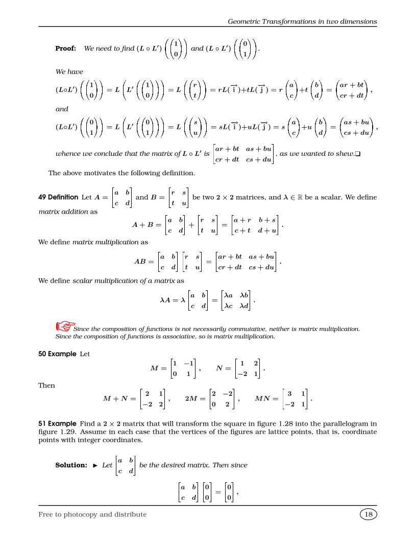
51 Example Find a 2× 2 matrix that will transform the square in figure 1.28 into the parallelogram infigure 1.29. Assume in each case that the vertices of the figures are lattice points, that is, coordinatepoints with integer coordinates.
Solution: I Let
"a b
c d
#be the desired matrix. Then since"
a b
c d
# "0
0
#=
"0
0
#,
Free to photocopy and distribute 18
Chapter 1
the point
0
0
!is a fortiori, transformed to itself. We now assume, without loss of generality,
that each vertex of the square is transformed in the same order, counterclockwise, to each
vertex of the rectangle. Then"a b
c d
# "1
0
#=
"2
2
#=⇒
"a
c
#=
"2
2
#=⇒ a = c = 2.
Using these values,"a b
c d
# "1
1
#=
"1
3
#=⇒
"a + b
c + d
#=
"1
3
#=⇒ b = −1, d = 1.
And so the desired matrix is "2 −1
2 1
#.
J
-4 -3 -2 -1 0 1 2 3 4 5-4
-3
-2
-1
0
1
2
3
4
5
Figure 1.28: Example 51.
-4 -3 -2 -1 0 1 2 3 4 5-4
-3
-2
-1
0
1
2
3
4
5
b
b
b
b
Figure 1.29: Example 51.
Homework
Problem 1.4.1 If A =
1 −1
2 3
, B =
a b
1 −2
and
(A + B)2 = A2 + 2AB + B2,
find a and b.
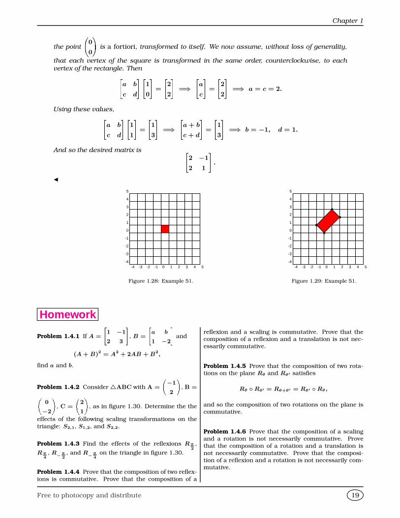
Problem 1.4.2 Consider4ABC with A =
−1
2
, B =
0
−2
, C =
2
1
, as in figure 1.30. Determine the the
effects of the following scaling transformations on the
triangle: S2,1, S1,2, and S2,2.
Problem 1.4.3 Find the effects of the reflexions R π2
,
R π4
, R− π2
, and R− π4
on the triangle in figure 1.30.
Problem 1.4.4 Prove that the composition of two reflex-
ions is commutative. Prove that the composition of a
reflexion and a scaling is commutative. Prove that thecomposition of a reflexion and a translation is not nec-essarily commutative.
Problem 1.4.5 Prove that the composition of two rota-tions on the plane Rθ and Rθ′ satisfies
Rθ Rθ′ = Rθ+θ′ = Rθ′ Rθ ,
and so the composition of two rotations on the plane iscommutative.
Problem 1.4.6 Prove that the composition of a scalingand a rotation is not necessarily commutative. Provethat the composition of a rotation and a translation is
not necessarily commutative. Prove that the composi-tion of a reflexion and a rotation is not necessarily com-mutative.
Free to photocopy and distribute 19
Determinants in two dimensions
Problem 1.4.7 Let L : R2 → R
2 and L′ : R2 → R
2
be linear transformations. Prove that their compositionL L′ is also a linear transformation.
-4 -3 -2 -1 0 1 2 3 4 5-4
-3
-2
-1
0
1
2
3
4
5
Figure 1.30: Problems 1.4.2, 1.4.8, and 1.4.3.
Problem 1.4.8 Find the effects of the reflexions RH ,
RV , and RO on the triangle in figure 1.30.
Problem 1.4.9 Find all matrices A ∈ M2×2(R) such
that A2 = 02
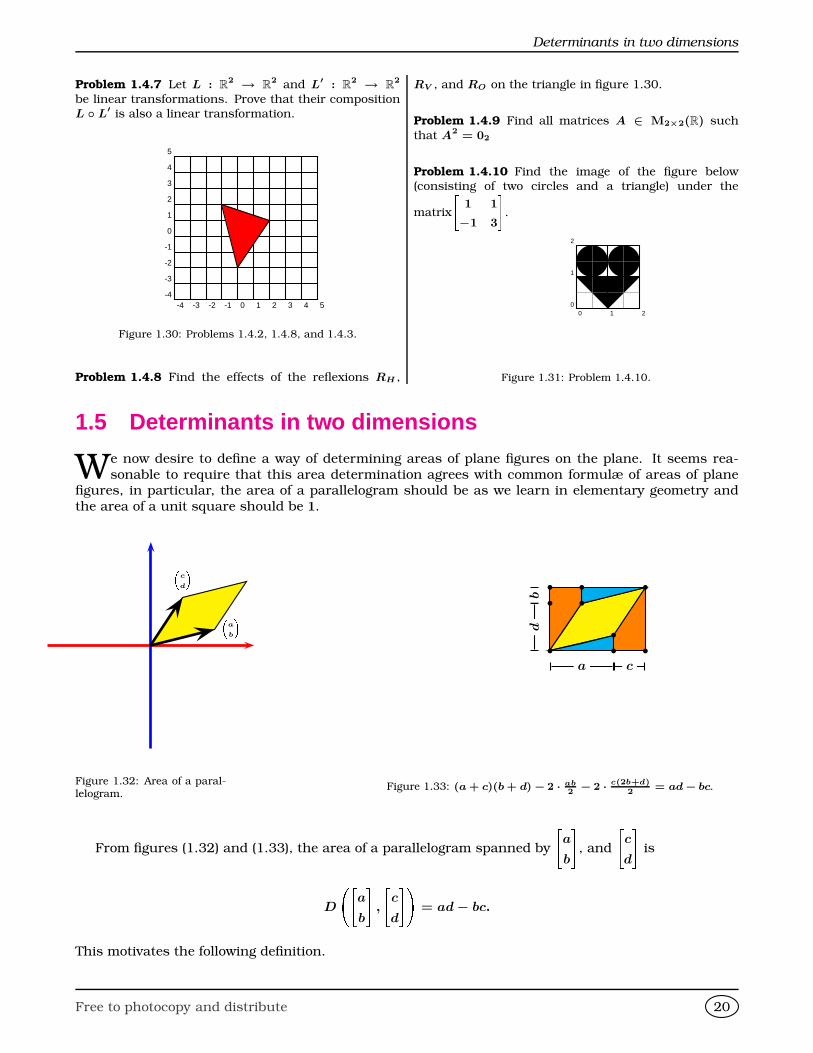
Problem 1.4.10 Find the image of the figure below(consisting of two circles and a triangle) under the
matrix
1 1
−1 3
.
0 1 20
1
2
Figure 1.31: Problem 1.4.10.
1.5 Determinants in two dimensions
We now desire to define a way of determining areas of plane figures on the plane. It seems rea-sonable to require that this area determination agrees with common formulæ of areas of plane
figures, in particular, the area of a parallelogram should be as we learn in elementary geometry andthe area of a unit square should be 1.
a
b
c
d
Figure 1.32: Area of a paral-lelogram.
b
b
b
b
b b
bb
b
d
a c
b
Figure 1.33: (a + c)(b + d) − 2 · ab2
− 2 · c(2b+d)2
= ad − bc.
From figures (1.32) and (1.33), the area of a parallelogram spanned by
"a
b
#, and
"c
d
#is
D
"a
b
#,
"c
d
#!= ad− bc.
This motivates the following definition.
Free to photocopy and distribute 20
Chapter 1
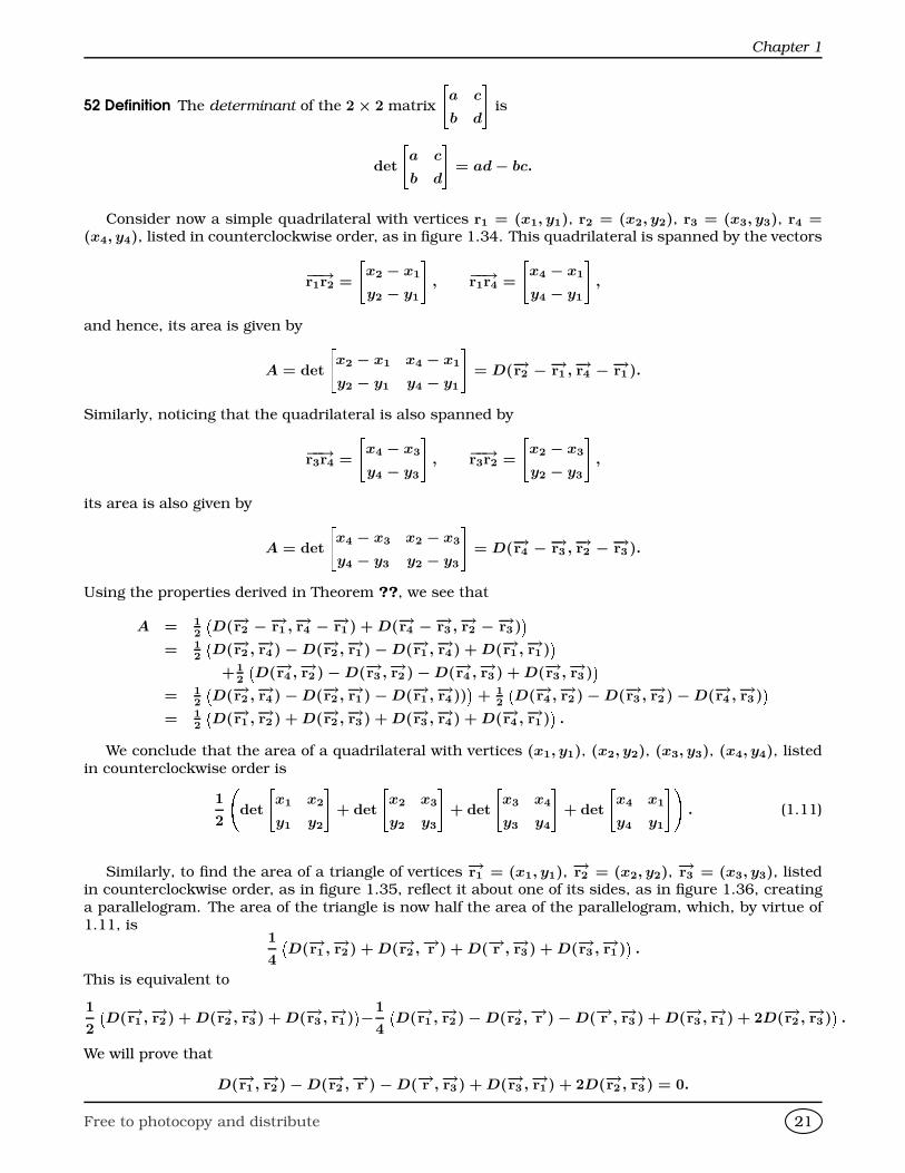
52 Definition The determinant of the 2× 2 matrix
"a c
b d
#is
det
"a c
b d
#= ad− bc.
Consider now a simple quadrilateral with vertices r1 = (x1, y1), r2 = (x2, y2), r3 = (x3, y3), r4 =(x4, y4), listed in counterclockwise order, as in figure 1.34. This quadrilateral is spanned by the vectors
−−→r1r2 =
"x2 − x1
y2 − y1
#, −−→r1r4 =
"x4 − x1
y4 − y1
#,
and hence, its area is given by
A = det
"x2 − x1 x4 − x1
y2 − y1 y4 − y1
#= D(−→r2 −−→r1 ,−→r4 −−→r1 ).
Similarly, noticing that the quadrilateral is also spanned by
−−→r3r4 =
"x4 − x3
y4 − y3
#, −−→r3r2 =
"x2 − x3
y2 − y3
#,
its area is also given by
A = det
"x4 − x3 x2 − x3
y4 − y3 y2 − y3
#= D(−→r4 −−→r3 ,−→r2 −−→r3 ).
Using the properties derived in Theorem ??, we see that
A = 12
D(−→r2 −−→r1 ,−→r4 −−→r1 ) + D(−→r4 −−→r3 ,−→r2 −−→r3 )
= 1
2
D(−→r2 ,−→r4 )−D(−→r2 ,−→r1 )−D(−→r1 ,−→r4 ) + D(−→r1 ,−→r1 )
+1
2
D(−→r4 ,−→r2 )−D(−→r3 ,−→r2 )−D(−→r4 ,−→r3 ) + D(−→r3 ,−→r3 )
= 1
2
D(−→r2 ,−→r4 )−D(−→r2 ,−→r1 )−D(−→r1 ,−→r4 ))
+ 1
2
D(−→r4 ,−→r2 )−D(−→r3 ,−→r2 )−D(−→r4 ,−→r3 )
= 1
2
D(−→r1 ,−→r2 ) + D(−→r2 ,−→r3 ) + D(−→r3 ,−→r4 ) + D(−→r4 ,−→r1 )
.
We conclude that the area of a quadrilateral with vertices (x1, y1), (x2, y2), (x3, y3), (x4, y4), listedin counterclockwise order is
1
2
det
"x1 x2
y1 y2
#+ det
"x2 x3
y2 y3
#+ det
"x3 x4
y3 y4
#+ det
"x4 x1
y4 y1
#!. (1.11)
Similarly, to find the area of a triangle of vertices −→r1 = (x1, y1),−→r2 = (x2, y2),
−→r3 = (x3, y3), listedin counterclockwise order, as in figure 1.35, reflect it about one of its sides, as in figure 1.36, creatinga parallelogram. The area of the triangle is now half the area of the parallelogram, which, by virtue of1.11, is
1
4
D(−→r1 ,−→r2 ) + D(−→r2 ,−→r ) + D(−→r ,−→r3 ) + D(−→r3 ,−→r1 )
.
This is equivalent to
1
2
D(−→r1 ,−→r2 ) + D(−→r2 ,−→r3 ) + D(−→r3 ,−→r1 )
−1
4
D(−→r1 ,−→r2 )−D(−→r2 ,−→r )−D(−→r ,−→r3 ) + D(−→r3 ,−→r1 ) + 2D(−→r2 ,−→r3 )
.
We will prove that
D(−→r1 ,−→r2 )−D(−→r2 ,−→r )−D(−→r ,−→r3 ) + D(−→r3 ,−→r1 ) + 2D(−→r2 ,−→r3 ) = 0.
Free to photocopy and distribute 21
Determinants in two dimensions
To do this, we appeal once again to the bi-linearity properties derived in Theorem ??, and observe, thatsince we have a parallelogram, −→r −−→r3 = −→r2 −−→r1 , which means −→r = −→r3 +−→r2 −−→r1 . Thus
D(−→r1 ,−→r2 )−D(−→r2 ,−→r )−D(−→r ,−→r3 ) + D(−→r3 ,−→r1 ) + 2D(−→r2 ,−→r3 ) = D(−→r1 ,−→r2 )−D(−→r2 ,−→r3 +−→r2 −−→r1 ) + 2D(−→r2 ,−→r3 )
−D(−→r3 +−→r2 −−→r1 ,−→r3 ) + D(−→r3 ,−→r1 )
= D(−→r1 ,−→r2 −−→r3 ) + D(−→r3 +−→r2 −−→r1 ,−→r2 −−→r3 )
+2D(−→r2 ,−→r3 )
= D(−→r3 +−→r2 ,−→r2 −−→r3 ) + 2D(−→r2 ,−→r3 )
= D(−→r3 ,−→r2 )−D(−→r2 ,−→r3 ) + 2D(−→r2 ,−→r3 )
= D(−→r3 ,−→r2 )−D(−→r2 ,−→r3 )
= 0,
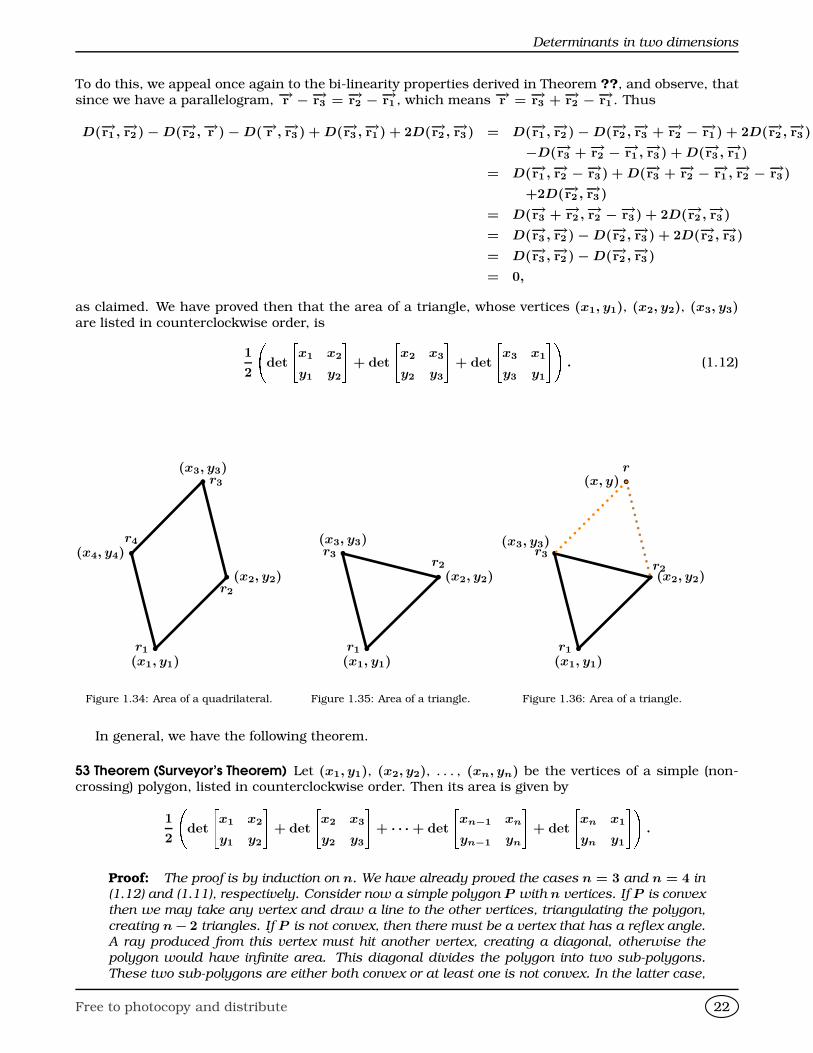
as claimed. We have proved then that the area of a triangle, whose vertices (x1, y1), (x2, y2), (x3, y3)are listed in counterclockwise order, is
1
2
det
"x1 x2
y1 y2
#+ det
"x2 x3
y2 y3
#+ det
"x3 x1
y3 y1
#!. (1.12)
br1
b
r2
b
r4
b r3
(x1, y1)
(x2, y2)
(x3, y3)
(x4, y4)
Figure 1.34: Area of a quadrilateral.
br1
b
r2
br3
(x1, y1)
(x2, y2)
(x3, y3)
Figure 1.35: Area of a triangle.
br1
br2
br3
b
r
(x1, y1)
(x2, y2)
(x3, y3)
(x, y)
Figure 1.36: Area of a triangle.
In general, we have the following theorem.
53 Theorem (Surveyor’s Theorem) Let (x1, y1), (x2, y2), . . . , (xn, yn) be the vertices of a simple (non-crossing) polygon, listed in counterclockwise order. Then its area is given by
1
2
det
"x1 x2
y1 y2
#+ det
"x2 x3
y2 y3
#+ · · ·+ det
"xn−1 xn
yn−1 yn
#+ det
"xn x1
yn y1
#!.
Proof: The proof is by induction on n. We have already proved the cases n = 3 and n = 4 in
(1.12) and (1.11), respectively. Consider now a simple polygon P with n vertices. If P is convex
then we may take any vertex and draw a line to the other vertices, triangulating the polygon,
creating n− 2 triangles. If P is not convex, then there must be a vertex that has a reflex angle.
A ray produced from this vertex must hit another vertex, creating a diagonal, otherwise the
polygon would have infinite area. This diagonal divides the polygon into two sub-polygons.
These two sub-polygons are either both convex or at least one is not convex. In the latter case,
Free to photocopy and distribute 22
Chapter 1
we repeat the argument, finding another diagonal and creating a new sub-polygon. Eventually,
since the number of vertices is infinite, we end up triangulating the polygon. Moreover, the
polygon can be triangulated in such a way that all triangles inherit the positive orientation of the
original polygon but each neighbouring pair of triangles have opposite orientations. Applying
(1.12) we obtain that the area is Xdet
"xi xj
yi yj
#,
where the sum is over each oriented edge. Since each diagonal occurs twice, but having oppo-
site orientations, the terms
det
"xi xj
yi yj
#+ det
"xj xi
yj yi
#= 0,
disappear from the sum and we are simply left with
1
2
det
"x1 x2
y1 y2
#+ det
"x2 x3
y2 y3
#+ · · ·+ det
"xn−1 xn
yn−1 yn
#+ det
"xn x1
yn y1
#!.
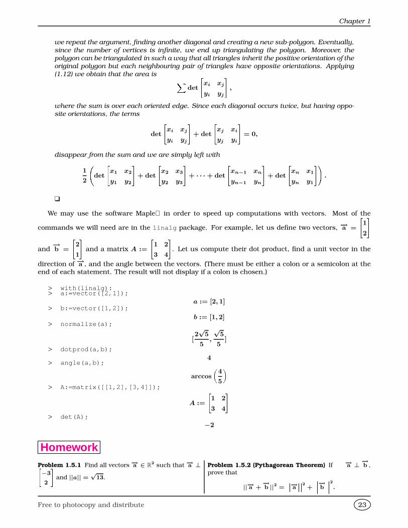
We may use the software Maple in order to speed up computations with vectors. Most of the
commands we will need are in the linalg package. For example, let us define two vectors, −→a =
"1
2
#and−→b =
"2
1
#and a matrix A :=
"1 2
3 4
#. Let us compute their dot product, find a unit vector in the
direction of −→a , and the angle between the vectors. (There must be either a colon or a semicolon at theend of each statement. The result will not display if a colon is chosen.)
> with(linalg):> a:=vector([2,1]);
a := [2, 1]> b:=vector([1,2]);
b := [1, 2]> normalize(a);
[2√
5
5,
√5
5]
> dotprod(a,b);4
> angle(a,b);
arccos
4
5
> A:=matrix([[1,2],[3,4]]);
A :=
"1 2
3 4
#> det(A);
−2
HomeworkProblem 1.5.1 Find all vectors −→a ∈ R
2 such that −→a ⊥−3
2
and ||a|| =
√13.
Problem 1.5.2 (Pythagorean Theorem) If −→a ⊥ −→b ,
prove that
||−→a +−→b ||2 =
−→a 2 +−→b 2.
Free to photocopy and distribute 23
Parametric Curves on the Plane
Problem 1.5.3 Let a, b be arbitrary real numbers.Prove that
(a2 + b2)2 ≤ 2(a4 + b4).
Problem 1.5.4 Let −→a ,−→b be fixed vectors in R
2. Prove
that if∀−→v ∈ R
2,−→v • −→a = −→v • −→b ,
then−→a =−→b .
Problem 1.5.5 (Polarisation Identity) Let −→u ,−→v be
vectors in R2. Prove that
−→u • −→v =1
4
||−→u +−→v ||2 − ||−→u − −→v ||2
.
Problem 1.5.6 Consider two lines on the plane L1 and
L2 with Cartesian equations L1 : y = m1x + b1 andL2 : y = m2x + b1, where m1 6= 0, m2 6= 0. UsingCorollary 22, prove that L1 ⊥ L2 ⇐⇒ m1m2 = −1. .
Problem 1.5.7 Find the Cartesian equation of all lines
L′ passing through
−1
2
and making an angle of
π
6
radians with the Cartesian line L : x + y = 1.
Problem 1.5.8 Let −→v , −→w , be vectors on the plane, with
−→w 6= −→0 . Prove that the vector −→a = −→v −−→v •−→w−→w 2−→w is
perpendicular to −→w .
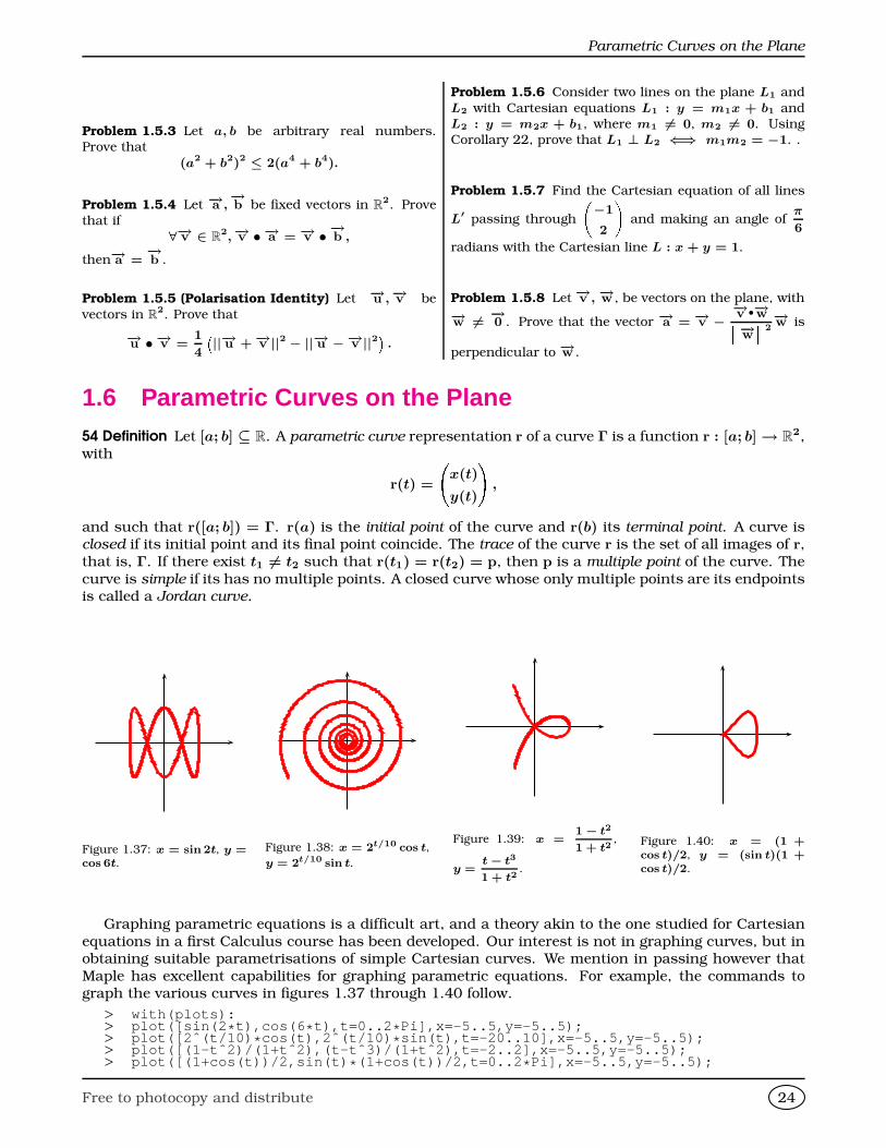
1.6 Parametric Curves on the Plane54 Definition Let [a; b] ⊆ R. A parametric curve representation r of a curve Γ is a function r : [a; b]→ R
2,with
r(t) =
x(t)
y(t)
!,
and such that r([a; b]) = Γ. r(a) is the initial point of the curve and r(b) its terminal point. A curve isclosed if its initial point and its final point coincide. The trace of the curve r is the set of all images of r,that is, Γ. If there exist t1 6= t2 such that r(t1) = r(t2) = p, then p is a multiple point of the curve. Thecurve is simple if its has no multiple points. A closed curve whose only multiple points are its endpointsis called a Jordan curve.
Figure 1.37: x = sin 2t, y =cos 6t.
Figure 1.38: x = 2t/10 cos t,
y = 2t/10 sin t.
Figure 1.39: x =1 − t2
1 + t2,
y =t − t3
1 + t2.
Figure 1.40: x = (1 +cos t)/2, y = (sin t)(1 +cos t)/2.
Graphing parametric equations is a difficult art, and a theory akin to the one studied for Cartesianequations in a first Calculus course has been developed. Our interest is not in graphing curves, but inobtaining suitable parametrisations of simple Cartesian curves. We mention in passing however thatMaple has excellent capabilities for graphing parametric equations. For example, the commands tograph the various curves in figures 1.37 through 1.40 follow.
> with(plots):> plot([sin(2 * t),cos(6 * t),t=0..2 * Pi],x=-5..5,y=-5..5);> plot([2ˆ(t/10) * cos(t),2ˆ(t/10) * sin(t),t=-20..10],x=-5..5,y=-5..5);> plot([(1-tˆ2)/(1+tˆ2),(t-tˆ3)/(1+tˆ2),t=-2..2],x=-5 ..5,y=-5..5);> plot([(1+cos(t))/2,sin(t) * (1+cos(t))/2,t=0..2 * Pi],x=-5..5,y=-5..5);
Free to photocopy and distribute 24
Chapter 1
Our main focus of attention will be the following. Given a Cartesian curve with equation f(x, y) = 0,we wish to find suitable parametrisations for them. That is, we want to find functions x : t 7→ a(t),y : t 7→ b(t) and an interval I such that the graphs of f(x, y) = 0 and f(a(t), b(t)) = 0, t ∈ I coincide.These parametrisations may differ in features, according to the choice of functions and the choice ofintervals.
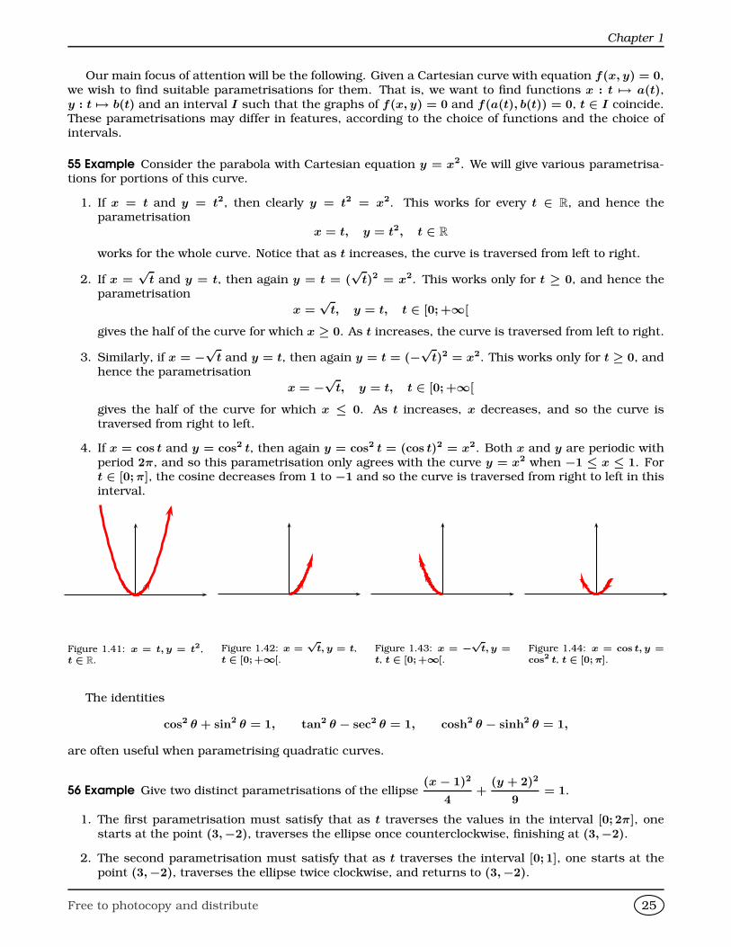
55 Example Consider the parabola with Cartesian equation y = x2. We will give various parametrisa-tions for portions of this curve.
1. If x = t and y = t2, then clearly y = t2 = x2. This works for every t ∈ R, and hence theparametrisation
x = t, y = t2, t ∈ R
works for the whole curve. Notice that as t increases, the curve is traversed from left to right.
2. If x =√
t and y = t, then again y = t = (√
t)2 = x2. This works only for t ≥ 0, and hence theparametrisation
x =√
t, y = t, t ∈ [0;+∞[
gives the half of the curve for which x ≥ 0. As t increases, the curve is traversed from left to right.
3. Similarly, if x = −√
t and y = t, then again y = t = (−√
t)2 = x2. This works only for t ≥ 0, andhence the parametrisation
x = −√
t, y = t, t ∈ [0;+∞[
gives the half of the curve for which x ≤ 0. As t increases, x decreases, and so the curve istraversed from right to left.
4. If x = cos t and y = cos2 t, then again y = cos2 t = (cos t)2 = x2. Both x and y are periodic withperiod 2π, and so this parametrisation only agrees with the curve y = x2 when −1 ≤ x ≤ 1. Fort ∈ [0; π], the cosine decreases from 1 to −1 and so the curve is traversed from right to left in thisinterval.
Figure 1.41: x = t, y = t2,t ∈ R.
Figure 1.42: x =√
t, y = t,t ∈ [0;+∞[.
Figure 1.43: x = −√
t, y =t, t ∈ [0;+∞[.
Figure 1.44: x = cos t, y =cos2 t, t ∈ [0; π].
The identities
cos2 θ + sin2 θ = 1, tan2 θ − sec2 θ = 1, cosh2 θ − sinh2 θ = 1,
are often useful when parametrising quadratic curves.
56 Example Give two distinct parametrisations of the ellipse(x − 1)2
4+
(y + 2)2
9= 1.
1. The first parametrisation must satisfy that as t traverses the values in the interval [0; 2π], onestarts at the point (3,−2), traverses the ellipse once counterclockwise, finishing at (3,−2).
2. The second parametrisation must satisfy that as t traverses the interval [0; 1], one starts at thepoint (3,−2), traverses the ellipse twice clockwise, and returns to (3,−2).
Free to photocopy and distribute 25
Parametric Curves on the Plane
Solution: I What formula do we know where a sum of two squares equals 1? We use a
trigonometric substitution, a sort of “polar coordinates.” Observe that for t ∈ [0; 2π], the point
(cos t, sin t) traverses the unit circle once, starting at (1, 0) and ending there. Put
x− 1
2= cos t =⇒ x = 1 + 2 cos t,
andy + 2
3= sin t =⇒ y = −2 + 3 sin t.
Then
x = 1 + 2 cos t, y = −2 + 3 sin t, t ∈ [0; 2π]
is the desired first parametrisation.
For the second parametrisation, notice that as t traverses the interval [0; 1], (sin 4πt, cos 4πt)traverses the unit interval twice, clockwise, but begins and ends at the point (0, 1). To begin at
the point (1, 0) we must make a shift:sin
4πt +
π
2
, cos
4πt +
π
2
will start at (1, 0) and
travel clockwise twice, as t traverses [0; 1]. Hence we may take
x = 1 + 2 sin4πt +
π
2
, y = −2 + 3 cos
4πt +
π
2
, t ∈ [0; 1]
as our parametrisation. J
Some classic curves can be described by mechanical means, as the curves drawn by a spirograph.We will consider one such curve.
b
O
bO′
b
Bb
P
φ
b
A
θ
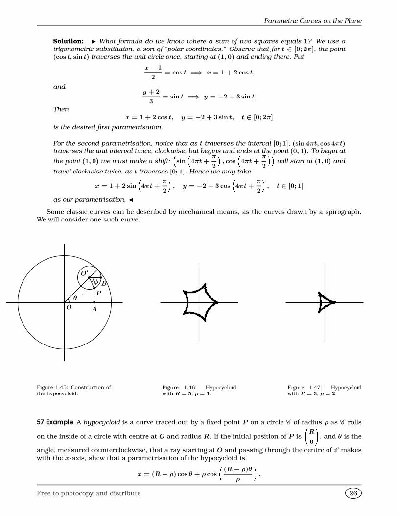
Figure 1.45: Construction ofthe hypocycloid.
Figure 1.46: Hypocycloidwith R = 5, ρ = 1.
Figure 1.47: Hypocycloidwith R = 3, ρ = 2.
57 Example A hypocycloid is a curve traced out by a fixed point P on a circle C of radius ρ as C rolls
on the inside of a circle with centre at O and radius R. If the initial position of P is
R
0
!, and θ is the
angle, measured counterclockwise, that a ray starting at O and passing through the centre of C makeswith the x-axis, shew that a parametrisation of the hypocycloid is
x = (R− ρ) cos θ + ρ cos
(R− ρ)θ
ρ
,
Free to photocopy and distribute 26
Chapter 1
y = (R− ρ) sin θ − ρ sin
(R− ρ)θ
ρ
.
Solution: I Suppose that starting from θ = 0, the centre O′ of the small circle moves coun-
terclockwise inside the larger circle by an angle θ, and the point P = (x, y) moves clockwise
an angle φ. The arc length travelled by the centre of the small circle is (R−ρ)θ radians. At the
same time the point P has rotated ρφ radians, and so (R − ρ)θ = ρφ. See figure 1.45, where
O′B is parallel to the x-axis.
Let A be the projection of P on the x-axis. Then ∠OAP = ∠OPO′ =π
2, ∠OO′P = π − φ− θ,
∠POA =π
2− φ, and OP = (R − ρ) sin(π − φ− θ). Hence
x = (OP ) cos ∠POA = (R− ρ) sin(π − φ− θ) cos(π
2− φ),
y = (R− ρ) sin(π − φ− θ) sin(π
2− φ).
Now
x = (R− ρ) sin(π − φ− θ) cos(π
2− φ)
= (R− ρ) sin(φ + θ) sin φ
=(R− ρ)
2(cos θ − cos(2φ + θ))
= (R− ρ) cos θ − (R− ρ)
2(cos θ + cos(2φ + θ))
= (R− ρ) cos θ − (R− ρ)(cos(θ + φ) cos φ).
Also, cos(θ + φ) = − cos(π − θ − φ) = − ρ
OO′ = − ρ
R − ρand cos φ = cos
(R− ρ)θ
ρ
and
so
x = (R− ρ) cos θ − (R− ρ)(cos(θ + φ) cos φ = (R− ρ) cos θ + ρ cos
(R− ρ)θ
ρ
,
as required. The identity for y is proved similarly. A particular example appears in figure 1.47.
J
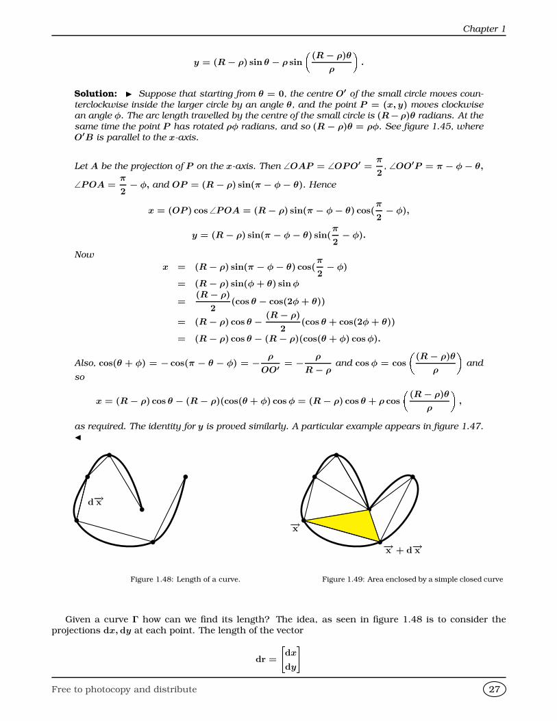
b
b
b
b
b
b
d−→x
Figure 1.48: Length of a curve.
b
b
b
b
b
b
−→x + d−→x
−→x
Figure 1.49: Area enclosed by a simple closed curve
Given a curve Γ how can we find its length? The idea, as seen in figure 1.48 is to consider theprojections dx, dy at each point. The length of the vector
dr =
"dx
dy
#Free to photocopy and distribute 27
Parametric Curves on the Plane
is
||dr|| =È
(dx)2 + (dy)2.
Hence the length of Γ is given by ZΓ||dr|| =
ZΓ
È(dx)2 + (dy)2. (1.13)
Similarly, suppose that Γ is a simple closed curve in R2. How do we find the (oriented) area of
the region it encloses? The idea, borrowed from finding areas of polygons, is to split the region intotriangles, each of area
1
2det
"x x + dx
y y + dy
#=
1
2det
"x dx
y dy
#=
1
2(xdy − ydx),
and to sum over the closed curve, obtaining a total oriented area of
1
2
IΓ
det
"x dx
y dy
#=
1
2
IΓ
(xdy − ydx). (1.14)
Here
IΓ
denotes integration around the closed curve.
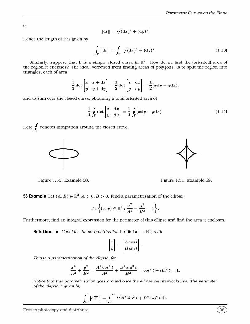
Figure 1.50: Example 58. Figure 1.51: Example 59.
58 Example Let (A, B) ∈ R2, A > 0, B > 0. Find a parametrisation of the ellipse
Γ :
(x, y) ∈ R
2 :x2
A2+
y2
B2= 1
.
Furthermore, find an integral expression for the perimeter of this ellipse and find the area it encloses.
Solution: I Consider the parametrisation Γ : [0; 2π]→ R2, with"
x
y
#=
"A cos t
B sin t
#.
This is a parametrisation of the ellipse, for
x2
A2+
y2
B2=
A2 cos2 t
A2+
B2 sin2 t
B2= cos2 t + sin2 t = 1.
Notice that this parametrisation goes around once the ellipse counterclockwise. The perimeter
of the ellipse is given by ZΓ
d−→r = Z 2π
0
ÈA2 sin2 t + B2 cos2 t dt.
Free to photocopy and distribute 28
Chapter 1
The above integral is an elliptic integral, and we do not have a closed form for it (in terms of
the elementary functions studied in Calculus I). We will have better luck with the area of the
ellipse, which is given by
1
2
IΓ(xdy − ydx) =
1
2
I(A cos t d(B sin t)−B sin t d(A cos t))
=1
2
Z 2π
0(AB cos2 t + AB sin2 t)) dt
=1
2
Z 2π
0AB dt
= πAB.
.
J
59 Example Find a parametric representation for the astroid
Γ :¦(x, y) ∈ R
2 : x2/3 + y2/3 = 1©
,
in figure 1.51. Find the perimeter of the astroid and the area it encloses.
Solution: I Take "x
y
#=
"cos3 t
sin3 t
#with t ∈ [0; 2π]. Then
x2/3 + y2/3 = cos2 t + sin2 t = 1.
The perimeter of the astroid isZΓ||dr|| =
Z 2π
0
È9 cos4 t sin2 t + 9 sin4 t cos2 t dt
=
Z 2π
03| sin t cos t| dt
=3
2
Z 2π
0
| sin 2t| dt
= 6
Z π/2
0
sin 2t dt
= 6.
The area of the astroid is given by
1
2
IΓ(xdy − ydx) =
1
2
I(cos3 t d(sin3 t)− sin3 t d(cos3 t))
=1
2
Z 2π
0(3 cos4 t sin2 t + 3 sin4 t cos2 t)) dt
=3
2
Z 2π
0
(sin t cos t)2 dt
=3
8
Z 2π
0
(sin 2t)2 dt
=3
16
Z 2π
0(1− cos 4t) dt
=3π
8.
We can use Maple (at least version 10) to calculate the above integrals. For example, if
(x, y) = (cos3 t, sin3 t), to compute the arc length we use the path integral command and to
compute the area, we use the line integral command with the vector field
"−y/2
x/2
#.
Free to photocopy and distribute 29
Parametric Curves on the Plane
> with(Student[VectorCalculus]):> PathInt( 1, [x,y]=Path( <(cos(t))ˆ3,(sin(t))ˆ3>,0..2 * Pi));> LineInt( VectorField(<-y/2,x/2>), Path( <(cos(t))ˆ3,(s in(t))ˆ3>,0..2 * Pi));
J
We include here for convenience, some Maple commands to compute various arc lengths and areas.
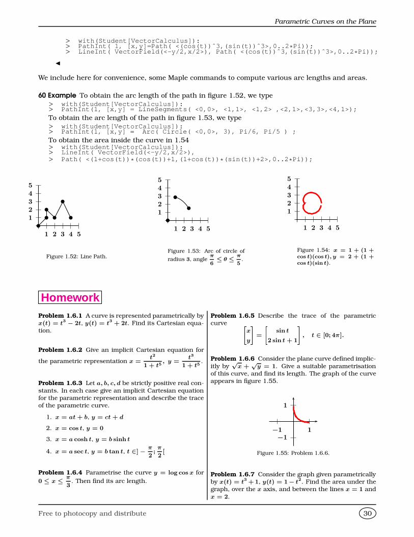
60 Example To obtain the arc length of the path in figure 1.52, we type> with(Student[VectorCalculus]):> PathInt(1, [x,y] = LineSegments( <0,0>, <1,1>, <1,2> ,<2,1 >,<3,3>,<4,1>);To obtain the arc length of the path in figure 1.53, we type> with(Student[VectorCalculus]):> PathInt(1, [x,y] = Arc( Circle( <0,0>, 3), Pi/6, Pi/5 ) ;To obtain the area inside the curve in 1.54> with(Student[VectorCalculus]):> LineInt( VectorField(<-y/2,x/2>),> Path( <(1+cos(t)) * (cos(t))+1,(1+cos(t)) * (sin(t))+2>,0..2 * Pi));
12345
1 2 3 4 5
b
b
b
b
b
b
Figure 1.52: Line Path.
12345
1 2 3 4 5
b
b
b
Figure 1.53: Arc of circle of
radius 3, angleπ
6≤ θ ≤ π
5.
12345
1 2 3 4 5
Figure 1.54: x = 1 + (1 +cos t)(cos t), y = 2 + (1 +cos t)(sin t).
HomeworkProblem 1.6.1 A curve is represented parametrically byx(t) = t3 − 2t, y(t) = t3 + 2t. Find its Cartesian equa-tion.
Problem 1.6.2 Give an implicit Cartesian equation for
the parametric representation x =t2
1 + t5, y =
t3
1 + t5.
Problem 1.6.3 Let a, b, c, d be strictly positive real con-
stants. In each case give an implicit Cartesian equationfor the parametric representation and describe the traceof the parametric curve.
1. x = at + b, y = ct + d
2. x = cos t, y = 0
3. x = a cosh t, y = b sinh t
4. x = a sec t, y = b tan t, t ∈]− π
2;π
2[
Problem 1.6.4 Parametrise the curve y = log cos x for
0 ≤ x ≤ π
3. Then find its arc length.
Problem 1.6.5 Describe the trace of the parametriccurve
x
y
=
sin t
2 sin t + 1
, t ∈ [0; 4π].
Problem 1.6.6 Consider the plane curve defined implic-
itly by√
x +√
y = 1. Give a suitable parametrisationof this curve, and find its length. The graph of the curveappears in figure 1.55.
1
−11−1
Figure 1.55: Problem 1.6.6.
Problem 1.6.7 Consider the graph given parametricallyby x(t) = t3 +1, y(t) = 1− t2. Find the area under thegraph, over the x axis, and between the lines x = 1 and
x = 2.
Free to photocopy and distribute 30
Chapter 1
Problem 1.6.8 Find the arc length of the curve given
parametrically by x(t) = 3t2, y(t) = 2t3 for 0 ≤ t ≤ 1.
Problem 1.6.9 Let C be the curve in R2 defined by
x(t) =t2
2, y(t) =
(2t + 1)3/2
3, t ∈ [−1
2;+
1
2].
Find the length of this curve.
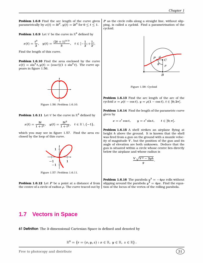
Problem 1.6.10 Find the area enclosed by the curvex(t) = sin3 t, y(t) = (cos t)(1 + sin2 t). The curve ap-pears in figure 1.56.
Figure 1.56: Problem 1.6.10.
Problem 1.6.11 Let C be the curve in R2 defined by
x(t) =3t
1 + t3, y(t) =
3t2
1 + t3, t ∈ R \ −1,
which you may see in figure 1.57. Find the area en-closed by the loop of this curve.
1
−11−1
Figure 1.57: Problem 1.6.11.
Problem 1.6.12 Let P be a point at a distance d fromthe centre of a circle of radius ρ. The curve traced out by
P as the circle rolls along a straight line, without slip-
ping, is called a cycloid. Find a parametrisation of thecycloid.
b
b CbP
b
B
ρ
d
θ
Figure 1.58: Cycloid
Problem 1.6.13 Find the arc length of the arc of the
cycloid x = ρ(t − cos t), y = ρ(1− cos t), t ∈ [0; 2π].
Problem 1.6.14 Find the length of the parametric curve
given by
x = et cos t, y = et sin t, t ∈ [0; π].
Problem 1.6.15 A shell strikes an airplane flying atheight h above the ground. It is known that the shellwas fired from a gun on the ground with a muzzle veloc-
ity of magnitude V , but the position of the gun and itsangle of elevation are both unknown. Deduce that thegun is situated within a circle whose centre lies directly
below the airplane and whose radius is
Vp
V 2 − 2gh
g.
Problem 1.6.16 The parabola y2 = −4px rolls withoutslipping around the parabola y2 = 4px. Find the equa-tion of the locus of the vertex of the rolling parabola.
1.7 Vectors in Space
61 Definition The 3-dimensional Cartesian Space is defined and denoted by
R3 = r = (x, y, z) : x ∈ R, y ∈ R, z ∈ R .
Free to photocopy and distribute 31
Vectors in Space
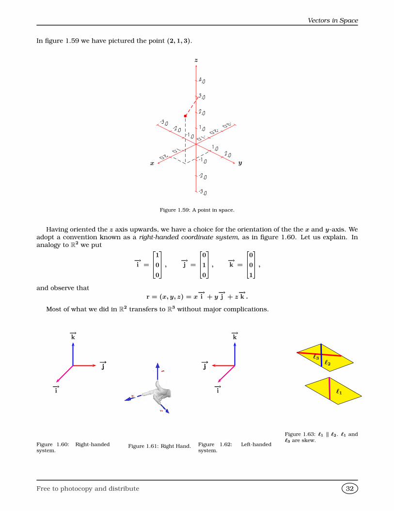
In figure 1.59 we have pictured the point (2, 1, 3).
x y
z
1.02.0
-1.0
-2.0
-3.0
1.02.0
-1.0
-2.0
-3.01.0
2.0
3.0
4.0
-1.0
-2.0
-3.0
b
Figure 1.59: A point in space.
Having oriented the z axis upwards, we have a choice for the orientation of the the x and y-axis. Weadopt a convention known as a right-handed coordinate system, as in figure 1.60. Let us explain. Inanalogy to R
2 we put
−→i =
264100
375 ,−→j =
264010
375 ,−→k =
264001
375 ,
and observe that
r = (x, y, z) = x−→i + y
−→j + z
−→k .
Most of what we did in R2 transfers to R
3 without major complications.
−→j
−→k
−→i
−→j
Figure 1.60: Right-handedsystem.
Figure 1.61: Right Hand.
−→j
−→k
−→i
−→j
Figure 1.62: Left-handedsystem.
`1
`2
`3
Figure 1.63: `1 ‖ `2. `1 and`3 are skew.
Free to photocopy and distribute 32
Chapter 1
62 Definition The dot product of two vectors −→a and−→b in R
3 is
−→a •−→b = a1b1 + a2b2 + a3b3.
The norm of a vector −→a in R3 is−→a = p−→a •−→a =
È(a1)2 + (a2)2 + (a3)2.
Just as in R2, the dot product satisfies −→a •
−→b =
−→a −→b cos θ, where θ ∈ [0;π] is the convex angle
between the two vectors.The Cauchy-Schwarz-Bunyakovsky Inequality takes the form
|−→a •−→b | ≤
−→a −→b =⇒ |a1b1 + a2b2 + a3b3| ≤ (a21 + a2
2 + a23)
1/2(b21 + b2
2 + b23)
1/2,
equality holding if an only if the vectors are parallel.
63 Example Let x, y, z be positive real numbers such that x2 + 4y2 + 9z2 = 27. Maximise x + y + z.
Solution: I Since x, y, z are positive, |x + y + z| = x + y + z. By Cauchy’s Inequality,
|x+y+z| =x + 2y
1
2
+ 3z
1
3
≤ (x2+4y2+9z2)1/2
1 +
1
4+
1
9
1/2
=√
27
7
6
=
7√
3
2.
Equality occurs if and only if264 x
2y
3z
375 = λ
264 1
1/2
1/3
375 =⇒ x = λ, y =λ
4, z =
λ
9=⇒ λ2 +
λ2
4+
λ2
9= 27 =⇒ λ = ±18
√3
7.
Therefore for a maximum we take
x =18√
3
7, y =
9√
3
14, z =
2√
3
7.
J
64 Definition Let a be a point in R3 and let −→v 6= −→0 be a vector in R
3. The parametric line passingthrough a in the direction of −→v is the set¦
r ∈ R3 : r = a + t−→v
©.
65 Example Find the parametric equation of the line passing through
1
2
3
and
−2
−1
0
.
Solution: I The line follows the direction2641− (−2)
2− (−1)
3− 0
375 =
264333
375 .
The desired equation is x
y
z
=
1
2
3
+ t
264333
375 .
J
Free to photocopy and distribute 33
Vectors in Space
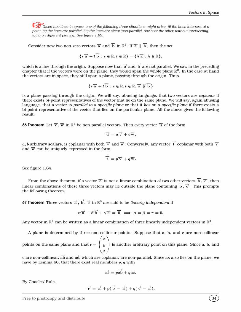
Given two lines in space, one of the following three situations might arise: (i) the lines intersect at a
point, (ii) the lines are parallel, (iii) the lines are skew (non-parallel, one over the other, without intersecting,
lying on different planes). See figure 1.63.
Consider now two non-zero vectors −→a and−→b in R
3. If −→a ‖ −→b , then the set
s−→a + t−→b : s ∈ R, t ∈ R = λ−→a : λ ∈ R,
which is a line through the origin. Suppose now that−→a and−→b are not parallel. We saw in the preceding
chapter that if the vectors were on the plane, they would span the whole plane R2. In the case at hand
the vectors are in space, they still span a plane, passing through the origin. Thus
s−→a + t−→b : s ∈ R, t ∈ R,−→a 6‖ −→b
is a plane passing through the origin. We will say, abusing language, that two vectors are coplanar ifthere exists bi-point representatives of the vector that lie on the same plane. We will say, again abusinglanguage, that a vector is parallel to a specific plane or that it lies on a specific plane if there exists abi-point representative of the vector that lies on the particular plane. All the above gives the followingresult.
66 Theorem Let −→v ,−→w in R3 be non-parallel vectors. Then every vector −→u of the form
−→u = a−→v + b−→w ,
a, b arbitrary scalars, is coplanar with both −→v and −→w . Conversely, any vector−→t coplanar with both −→v
and −→w can be uniquely expressed in the form
−→t = p−→v + q−→w .
See figure 1.64.
From the above theorem, if a vector −→a is not a linear combination of two other vectors−→b ,−→c , then
linear combinations of these three vectors may lie outside the plane containing−→b ,−→c . This prompts
the following theorem.
67 Theorem Three vectors −→a ,−→b ,−→c in R
3 are said to be linearly independent if
α−→a + β−→b + γ−→c =
−→0 =⇒ α = β = γ = 0.
Any vector in R3 can be written as a linear combination of three linearly independent vectors in R
3.
A plane is determined by three non-collinear points. Suppose that a, b, and c are non-collinear
points on the same plane and that r =
x
y
z
is another arbitrary point on this plane. Since a, b, and
c are non-collinear,−→ab and −→ac, which are coplanar, are non-parallel. Since −→ax also lies on the plane, we
have by Lemma 66, that there exist real numbers p, q with
−→ar = p−→ab + q−→ac.
By Chasles’ Rule,
−→r = −→a + p(−→b −−→a ) + q(−→c −−→a ),
Free to photocopy and distribute 34

Chapter 1
is the equation of a plane containing the three non-collinear points a, b, and c, where −→a ,−→b , and −→c
are the position vectors of these points. Thus we have the following theorem.
−→vp−→v + q−→w
−→w
Figure 1.64: Theorem 66.
ax + by + cz = d
−→x
−→n =
264a
b
c
375
Figure 1.65: Theorem 69.
68 Theorem Let −→u and −→v be linearly independent vectors. The parametric equation of a plane contain-ing the point a, and parallel to the vectors −→u and −→v is given by
−→r −−→a = p−→u + q−→v .
Componentwise this takes the form
x− a1 = pu1 + qv1,
y − a2 = pu2 + qv2,
z − a3 = pu3 + qv3.
Multiplying the first equation by u2v3−u3v2, the second by u3v1−u1v3, and the third by u1v2−u2v1,we obtain,
(u2v3 − u3v2)(x− a1) = (u2v3 − u3v2)(pu1 + qv1),
(u3v1 − u1v3)(y − a2) = (u3v1 − u1v3)(pu2 + qv2),
(u1v2 − u2v1)(z − a3) = (u1v2 − u2v1)(pu3 + qv3).
Adding gives,
(u2v3 − u3v2)(x− a1) + (u3v1 − u1v3)(y − a2) + (u1v2 − u2v1)(z − a3) = 0.
Puta = u2v3 − u3v2, b = u3v1 − u1v3, c = u1v2 − u2v1,
andd = a1(u2v3 − u3v2) + a2(u3v1 − u1v3) + a3(u1v2 − u2v1).
Since −→v is linearly independent from −→u , not all of a, b, c are zero. This gives the following theorem.
69 Theorem The equation of the plane in space can be written in the form
ax + by + cz = d,
which is the Cartesian equation of the plane. Here a2 + b2 + c2 6= 0, that is, at least one of the
coefficients is non-zero. Moreover, the vector −→n =
264a
b
c
375 is normal to the plane with Cartesian equation
ax + by + cz = d.
Free to photocopy and distribute 35
Vectors in Space
Proof: We have already proved the first statement. For the second statement, observe that
if −→u and −→v are non-parallel vectors and −→r − −→a = p−→u + q−→v is the equation of the plane
containing the point a and parallel to the vectors −→u and −→v , then if −→n is simultaneously per-
pendicular to −→u and −→v then (−→r −−→a )•−→n = 0 for −→u •−→n = 0 = −→v •−→n . Now, since at least one
of a, b, c is non-zero, we may assume a 6= 0. The argument is similar if one of the other letters
is non-zero and a = 0. In this case we can see that
x =d
a− b
ay − c
az.
Put y = s and z = t. Then x− d
ay
z
= s
2664− b
a1
0
3775+ t
2664− c
a0
1
3775is a parametric equation for the plane. We have
a
− b
a
+ b (1) + c (0) = 0, a
− c
a
+ b (0) + c (1) = 0,
and so
264a
b
c
375 is simultaneously perpendicular to
2664− b
a1
0
3775 and
2664− c
a0
1
3775, proving the second state-
ment.
70 Example The equation of the plane passing through the point
1
−1
2
and normal to the vector264−3
2
4
375 is
−3(x − 1) + 2(y + 1) + 4(z − 2) = 0 =⇒ −3x + 2y + 4z = 3.
71 Example Find both the parametric equation and the Cartesian equation of the plane parallel to the
vectors
264111
375 and
264110
375 and passing through the point
0
−1
2
.
Solution: I The desired parametric equation isx
y + 1
z − 2
= s
264111
375+ t
264110
375 .
This gives
s = z − 2, t = y + 1− s = y + 1− z + 2 = y − z + 3
and
x = s + t = z − 2 + y − z + 3 = y + 1.
Hence the Cartesian equation is x− y = 1. J
Free to photocopy and distribute 36
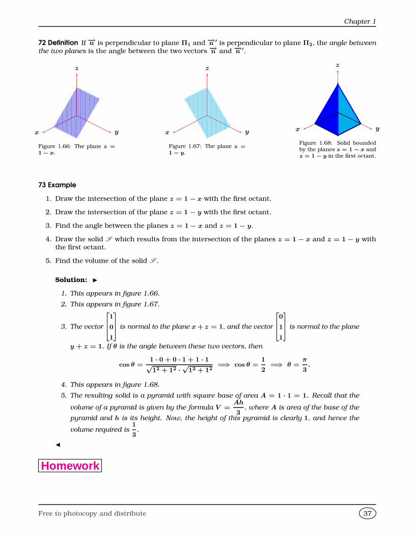
Chapter 1
72 Definition If −→n is perpendicular to plane Π1 and −→n ′ is perpendicular to plane Π2, the angle between
the two planes is the angle between the two vectors −→n and −→n ′.
x y
z
Figure 1.66: The plane z =1 − x.
x y
z
Figure 1.67: The plane z =1 − y.
x y
z
Figure 1.68: Solid boundedby the planes z = 1 − x andz = 1 − y in the first octant.
73 Example
1. Draw the intersection of the plane z = 1− x with the first octant.
2. Draw the intersection of the plane z = 1− y with the first octant.
3. Find the angle between the planes z = 1− x and z = 1− y.
4. Draw the solid S which results from the intersection of the planes z = 1− x and z = 1− y withthe first octant.
5. Find the volume of the solid S .
Solution: I
1. This appears in figure 1.66.
2. This appears in figure 1.67.
3. The vector
264101
375 is normal to the plane x + z = 1, and the vector
264011
375 is normal to the plane
y + z = 1. If θ is the angle between these two vectors, then
cos θ =1 · 0 + 0 · 1 + 1 · 1√12 + 12 ·
√12 + 12
=⇒ cos θ =1
2=⇒ θ =
π
3.
4. This appears in figure 1.68.
5. The resulting solid is a pyramid with square base of area A = 1 · 1 = 1. Recall that the
volume of a pyramid is given by the formula V =Ah
3, where A is area of the base of the
pyramid and h is its height. Now, the height of this pyramid is clearly 1, and hence the
volume required is1
3.
J
Homework
Free to photocopy and distribute 37
Vectors in Space
Problem 1.7.1 Vectors −→a ,−→b satisfy
−→a = 13,−→b = 19,
−→a +−→b = 24. Find
−→a − −→b .Problem 1.7.2 Find the equation of the line passing
through
1
2
3
DZin the direction of
264−2
−1
0
375.
Problem 1.7.3 Find the equation of plane containing
the point
1
1
1
DZand perpendicular to the line x =
1 + t, y = −2t, z = 1− t.
Problem 1.7.4 Find the equation of plane containing
the point
1
−1
−1
DZand containing the line x = 2y = 3z.
Problem 1.7.5 (Putnam Exam 1984) Let A be a solida × b × c rectangular brick in three dimensions, where
a > 0, b > 0, c > 0. Let B be the set of all pointswhich are at distance at most 1 from some point of A(in particular, A ⊆ B). Express the volume of B as apolynomial in a, b, c.
Problem 1.7.6 It is known that−→a = 3,
−→b = 4,−→c = 5 and that −→a +−→b + −→c =
−→0 . Find
−→a •−→b +
−→b •−→c +−→c •−→a .
Problem 1.7.7 Find the equation of the line perpendic-ular to the plane ax + a2y + a3z = 0, a 6= 0 and
passing through the point
0
0
1
DZ.
Problem 1.7.8 Find the equation of the plane perpen-
dicular to the line ax = by = cz, abc 6= 0 and passing
through the point
1
1
1
DZin R
3.
Problem 1.7.9 Find the (shortest) distance from thepoint (1, 2, 3) to the plane x − y + z = 1.
Problem 1.7.10 Determine whether the lines
L1 :
x
y
z
DZ=
1
1
1
DZ+ t
2642
1
1
375 ,
L2 :
x
y
z
DZ=
0
0
1
DZ+ t
264 2
−1
1
375 ,
intersect. Find the angle between them.
Problem 1.7.11 Let a, b, c be arbitrary real numbers.Prove that
(a2 + b2 + c2)2 ≤ 3(a4 + b4 + c4).
Problem 1.7.12 Let a > 0, b > 0, c > 0 be the
lengths of the sides of 4ABC. (Vertex A is oppo-site to the side measuring a, etc.) Recall that byHeron’s Formula, the area of this triangle is S(a, b, c) =È
s(s − a)(s − b)(s − c), where s =a + b + c
2is the
semiperimeter of the triangle. Prove that f(a, b, c) =S(a, b, c)
a2 + b2 + c2is maximised when 4ABC is equilateral,
and find this maximum.
Problem 1.7.13 Let x, y, z be strictly positive numbers.Prove that
√x + y +
√y + z +
√z + x√
x + y + z≤√
6.
Problem 1.7.14 Let x, y, z be strictly positive numbers.Prove that
x + y + z ≤ 2
x2
y + z+
y2
z + x+
z2
x + y
.
Problem 1.7.15 Find the Cartesian equation of the
plane passing through
1
0
0
DZ,
0
1
0
DZand
0
0
1
DZ. Draw
this plane and its intersection with the first octant. Find
the volume of the tetrahedron with vertices at
0
0
0
DZ,
1
0
0
DZ,
0
1
0
DZand
0
0
1
DZ.
Problem 1.7.16 Prove that there do not exist three unitvectors in R
3 such that the angle between any two of
them be >2π
3.
Problem 1.7.17 Let (−→r − −→a )•−→n = 0 be a plane pass-ing through the point a and perpendicular to vector −→n .If b is not a point on the plane, then the distance from
b to the plane is (−→a − −→b )•−→n−→n .
Free to photocopy and distribute 38
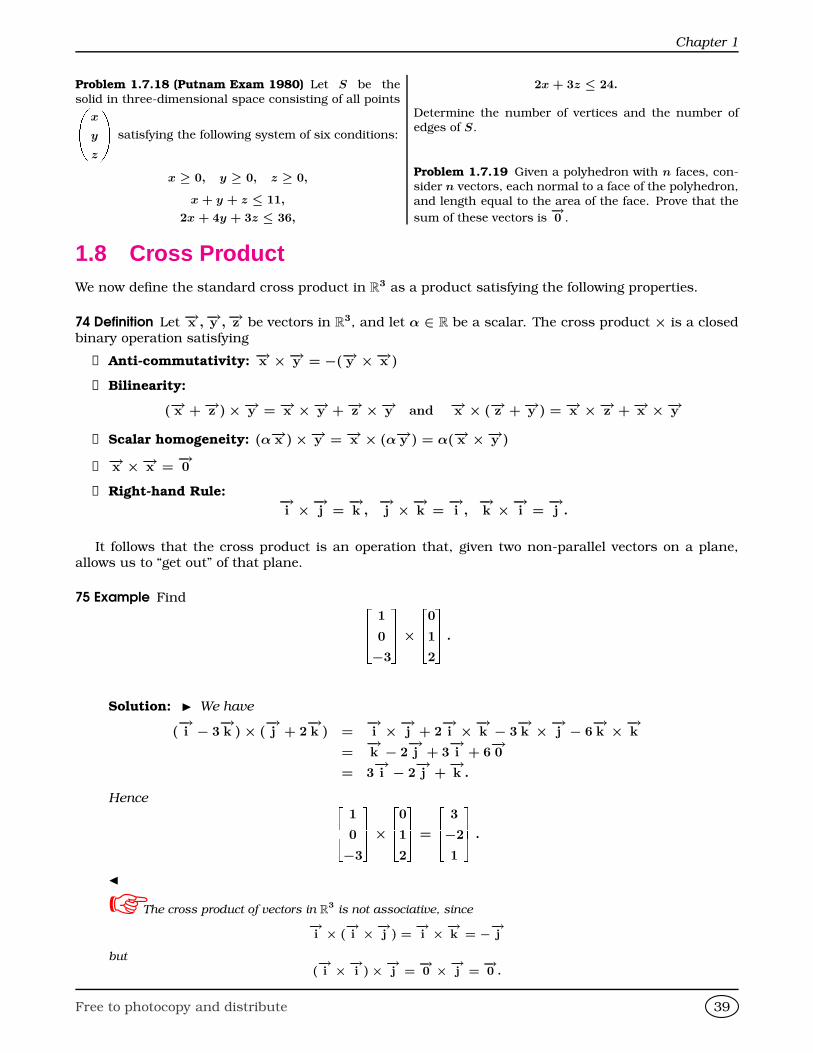
Chapter 1
Problem 1.7.18 (Putnam Exam 1980) Let S be the
solid in three-dimensional space consisting of all pointsx
y
z
DZsatisfying the following system of six conditions:
x ≥ 0, y ≥ 0, z ≥ 0,
x + y + z ≤ 11,
2x + 4y + 3z ≤ 36,
2x + 3z ≤ 24.
Determine the number of vertices and the number ofedges of S.
Problem 1.7.19 Given a polyhedron with n faces, con-sider n vectors, each normal to a face of the polyhedron,
and length equal to the area of the face. Prove that the
sum of these vectors is−→0 .
1.8 Cross ProductWe now define the standard cross product in R
3 as a product satisfying the following properties.
74 Definition Let −→x ,−→y ,−→z be vectors in R3, and let α ∈ R be a scalar. The cross product × is a closed
binary operation satisfying
➊ Anti-commutativity: −→x ×−→y = −(−→y ×−→x )
➋ Bilinearity:
(−→x +−→z )×−→y = −→x ×−→y +−→z ×−→y and −→x × (−→z +−→y ) = −→x ×−→z +−→x ×−→y
➌ Scalar homogeneity: (α−→x )×−→y = −→x × (α−→y ) = α(−→x ×−→y )
➍ −→x ×−→x =−→0
➎ Right-hand Rule: −→i ×−→j =
−→k ,−→j ×−→k =
−→i ,−→k ×−→i =
−→j .
It follows that the cross product is an operation that, given two non-parallel vectors on a plane,allows us to “get out” of that plane.
75 Example Find 264 1
0
−3
375× 264012
375 .
Solution: I We have
(−→i − 3
−→k )× (
−→j + 2
−→k ) =
−→i ×−→j + 2
−→i ×−→k − 3
−→k ×−→j − 6
−→k ×−→k
=−→k − 2
−→j + 3
−→i + 6
−→0
= 3−→i − 2
−→j +−→k .
Hence 264 1
0
−3
375× 264012
375 =
264 3
−2
1
375 .
J
The cross product of vectors in R3
is not associative, since
−→i × (
−→i × −→j ) =
−→i × −→k = −−→j
but
(−→i × −→i )× −→j =
−→0 × −→j =
−→0 .
Free to photocopy and distribute 39
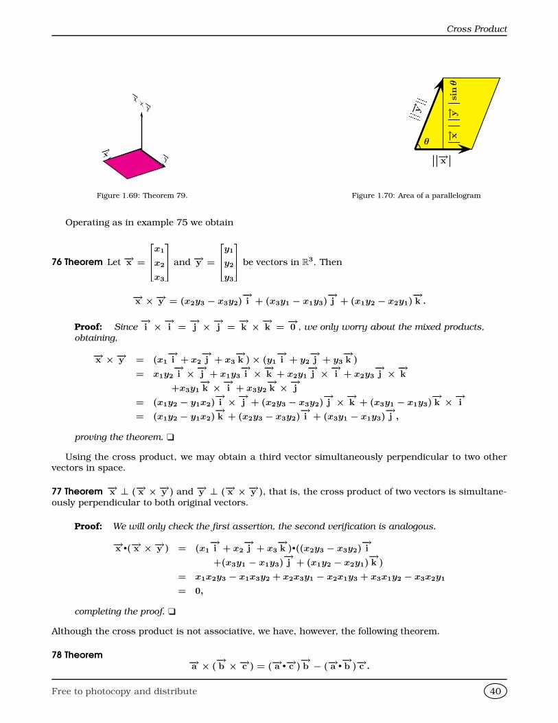
Cross Product
−→x ×−→
y
−→y
−→x
Figure 1.69: Theorem 79.
−→x −→ y θ −→ x −→ y sin
θ
Figure 1.70: Area of a parallelogram
Operating as in example 75 we obtain
76 Theorem Let −→x =
264x1
x2
x3
375 and −→y =
264y1
y2
y3
375 be vectors in R3. Then
−→x ×−→y = (x2y3 − x3y2)−→i + (x3y1 − x1y3)
−→j + (x1y2 − x2y1)
−→k .
Proof: Since−→i × −→i =
−→j × −→j =
−→k × −→k =
−→0 , we only worry about the mixed products,
obtaining,
−→x ×−→y = (x1−→i + x2
−→j + x3
−→k )× (y1
−→i + y2
−→j + y3
−→k )
= x1y2−→i ×−→j + x1y3
−→i ×−→k + x2y1
−→j ×−→i + x2y3
−→j ×−→k
+x3y1−→k ×−→i + x3y2
−→k ×−→j
= (x1y2 − y1x2)−→i ×−→j + (x2y3 − x3y2)
−→j ×−→k + (x3y1 − x1y3)
−→k ×−→i
= (x1y2 − y1x2)−→k + (x2y3 − x3y2)
−→i + (x3y1 − x1y3)
−→j ,
proving the theorem.
Using the cross product, we may obtain a third vector simultaneously perpendicular to two othervectors in space.
77 Theorem −→x ⊥ (−→x ×−→y ) and −→y ⊥ (−→x ×−→y ), that is, the cross product of two vectors is simultane-ously perpendicular to both original vectors.
Proof: We will only check the first assertion, the second verification is analogous.
−→x •(−→x ×−→y ) = (x1−→i + x2
−→j + x3
−→k )•((x2y3 − x3y2)
−→i
+(x3y1 − x1y3)−→j + (x1y2 − x2y1)
−→k )
= x1x2y3 − x1x3y2 + x2x3y1 − x2x1y3 + x3x1y2 − x3x2y1
= 0,
completing the proof.
Although the cross product is not associative, we have, however, the following theorem.
78 Theorem −→a × (−→b ×−→c ) = (−→a •−→c )
−→b − (−→a •
−→b )−→c .
Free to photocopy and distribute 40
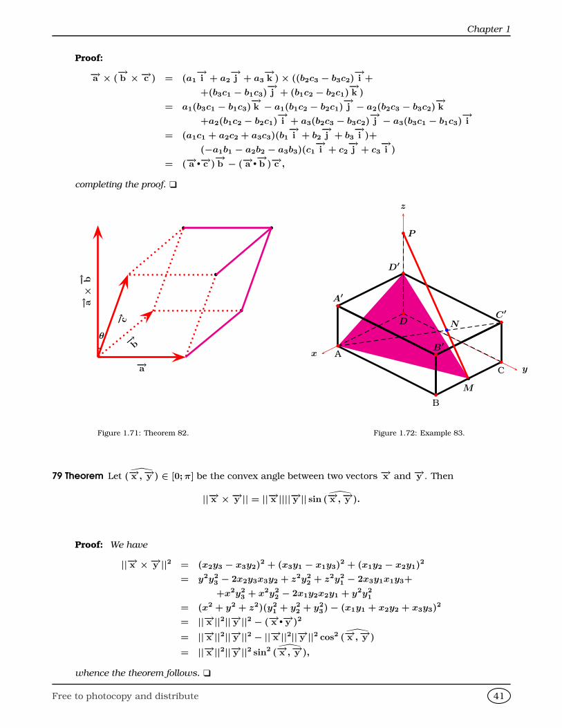
Chapter 1
Proof:
−→a × (−→b ×−→c ) = (a1
−→i + a2
−→j + a3
−→k )× ((b2c3 − b3c2)
−→i +
+(b3c1 − b1c3)−→j + (b1c2 − b2c1)
−→k )
= a1(b3c1 − b1c3)−→k − a1(b1c2 − b2c1)
−→j − a2(b2c3 − b3c2)
−→k
+a2(b1c2 − b2c1)−→i + a3(b2c3 − b3c2)
−→j − a3(b3c1 − b1c3)
−→i
= (a1c1 + a2c2 + a3c3)(b1−→i + b2
−→j + b3
−→i )+
(−a1b1 − a2b2 − a3b3)(c1−→i + c2
−→j + c3
−→i )
= (−→a •−→c )−→b − (−→a •
−→b )−→c ,
completing the proof.
−→a
−→ c
−→ a×−→ b
−→b
b
b
b b
θ
Figure 1.71: Theorem 82.
x
y
z
b
M
b
A
b
B
b
C
b
D
bA′
bB′
bN
bC′
bD′
b P
Figure 1.72: Example 83.
79 Theorem Let (−→x ,−→y ) ∈ [0; π] be the convex angle between two vectors −→x and −→y . Then
||−→x ×−→y || = ||−→x ||||−→y || sin (−→x ,−→y ).
Proof: We have
||−→x ×−→y ||2 = (x2y3 − x3y2)2 + (x3y1 − x1y3)
2 + (x1y2 − x2y1)2
= y2y23 − 2x2y3x3y2 + z2y2
2 + z2y21 − 2x3y1x1y3+
+x2y23 + x2y2
2 − 2x1y2x2y1 + y2y21
= (x2 + y2 + z2)(y21 + y2
2 + y23)− (x1y1 + x2y2 + x3y3)
2
= ||−→x ||2||−→y ||2 − (−→x •−→y )2
= ||−→x ||2||−→y ||2 − ||−→x ||2||−→y ||2 cos2 (−→x ,−→y )
= ||−→x ||2||−→y ||2 sin2 (−→x ,−→y ),
whence the theorem follows.
Free to photocopy and distribute 41
Cross Product
Theorem 79 has the following geometric significance:−→x ×−→y is the area of the parallelogram
formed when the tails of the vectors are joined. See figure 1.70.The following corollaries easily follow from Theorem 79.
80 Corollary Two non-zero vectors −→x ,−→y satisfy −→x ×−→y =−→0 if and only if they are parallel.
81 Corollary (Lagrange’s Identity)
||−→x ×−→y ||2 = ||x||2||y||2 − (−→x •−→y )2.
The following result mixes the dot and the cross product.
82 Theorem Let −→a ,−→b , −→c , be linearly independent vectors in R
3. The signed volume of the paral-
lelepiped spanned by them is (−→a ×−→b ) • −→c .
Proof: See figure 1.71. The area of the base of the parallelepiped is the area of the paral-
lelogram determined by the vectors −→a and−→b , which has area
−→a ×−→b . The altitude of the
parallelepiped is−→c cos θ where θ is the angle between −→c and −→a × −→b . The volume of the
parallelepiped is thus −→a ×−→b −→c cos θ = (−→a ×−→b ) • −→c ,
proving the theorem.
Since we may have used any of the faces of the parallelepiped, it follows that
(−→a × −→b ) • −→c = (−→b × −→c ) • −→a = (−→c × −→a ) • −→b .
In particular, it is possible to “exchange” the cross and dot products:
−→a • (−→b × −→c ) = (−→a × −→b ) • −→c
83 Example Consider the rectangular parallelepiped ABCDD′C′B′A′ (figure 1.72) with vertices A(2, 0, 0),B(2, 3, 0), C(0, 3, 0), D(0, 0, 0), D′(0, 0, 1), C′(0, 3, 1), B′(2, 3, 1), A′(2, 0, 1). Let M be the midpoint ofthe line segment joining the vertices B and C.
1. Find the Cartesian equation of the plane containing the points A, D′, and M .
2. Find the area of 4AD′M .
3. Find the parametric equation of the line←→AC′.
4. Suppose that a line through M is drawn cutting the line segment [AC′] in N and the line←−→DD′ in
P . Find the parametric equation of←→MP.
Solution: I
1. Form the following vectors and find their cross product:
−−→AD′ =
264−2
0
1
375 ,−−→AM =
264−1
3
0
375 =⇒−−→AD′ ×−−→AM =
264−3
−1
−6
375 .
The equation of the plane is thus264x− 2
y − 0
z − 0
375 • 264−3
−1
−6
375 = 0 =⇒ 3(x− 2) + 1(y) + 6z = 0 =⇒ 3x + y + 6z = 6.
Free to photocopy and distribute 42

Chapter 1
2. The area of the triangle is−−→AD′ ×−−→AM
2=
1
2
p32 + 12 + 62 =
√46
2.
3. We have−−→AC′ =
264−2
3
1
375, and hence the line←→AC′ has parametric equation
x
y
z
=
2
0
0
+ t
264−2
3
1
375 =⇒ x = 2− 2t, y = 3t, z = t.
4. Since P is on the z-axis, P =
0
0
z′
for some real number z′ > 0. The parametric
equation of the line←→MP is thus
x
y
z
=
1
3
0
+ s
264−1
−3
z′
375 =⇒ x = 1− s y = 3− 3s, z = sz′.
Since N is on both←→MP and
←→AC′ we must have
2− 2t = 1− s, 3t = 3− 3s, t = sz′.
Solving the first two equations gives s =1
3, t =
2
3. Putting this into the third equation we
deduce z′ = 2. Thus P =
0
0
2
and the desired equation is
x
y
z
=
1
3
0
+ s
264−1
−3
2
375 =⇒ x = 1− s, y = 3− 3s, z = 2s.
J
HomeworkProblem 1.8.1 Prove that
(−→a − −→b )× (−→a +−→b ) = 2−→a × −→b .
Problem 1.8.2 Prove that −→x ×−→x =−→0 follows from the
anti-commutativity of the cross product.
Problem 1.8.3 If−→b −−→a and −→c −−→a are parallel and it
is known that −→c ×−→a =−→i −−→j and −→a ×−→b =
−→j +−→k ,
find−→b × −→c .
Problem 1.8.4 Redo example 71, that is, find the Carte-
sian equation of the plane parallel to the vectors
2641
1
1
375and
2641
1
0
375 and passing through the point (0,−1, 2), by
finding a normal to the plane.
Free to photocopy and distribute 43
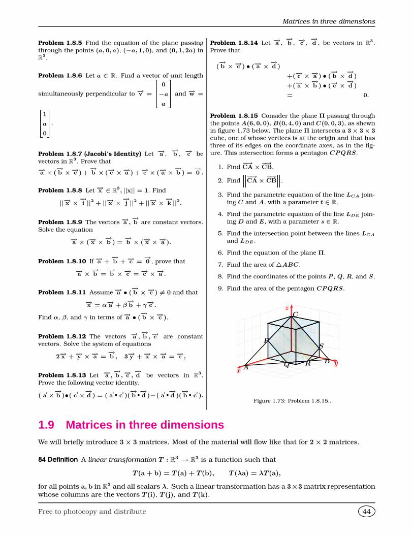
Matrices in three dimensions
Problem 1.8.5 Find the equation of the plane passing
through the points (a, 0, a), (−a, 1, 0), and (0, 1, 2a) inR
3.
Problem 1.8.6 Let a ∈ R. Find a vector of unit length
simultaneously perpendicular to −→v =
264 0
−a
a
375 and −→w =2641
a
0
375.
Problem 1.8.7 (Jacobi’s Identity) Let −→a ,−→b , −→c be
vectors in R3. Prove that
−→a × (−→b ×−→c ) +
−→b × (−→c ×−→a ) +−→c × (−→a ×−→b ) =
−→0 .
Problem 1.8.8 Let −→x ∈ R3, ||x|| = 1. Find
||−→x × −→i ||2 + ||−→x × −→j ||2 + ||−→x × −→k ||2.
Problem 1.8.9 The vectors −→a ,−→b are constant vectors.
Solve the equation
−→a × (−→x × −→b ) =−→b × (−→x × −→a ).
Problem 1.8.10 If −→a +−→b +−→c =
−→0 , prove that
−→a × −→b =−→b × −→c = −→c × −→a .
Problem 1.8.11 Assume −→a • (−→b × −→c ) 6= 0 and that
−→x = α−→a + β−→b + γ−→c .
Find α, β, and γ in terms of −→a • (−→b × −→c ).
Problem 1.8.12 The vectors −→a ,−→b ,−→c are constant
vectors. Solve the system of equations
2−→x +−→y × −→a =−→b , 3−→y +−→x × −→a = −→c ,
Problem 1.8.13 Let −→a ,−→b ,−→c ,
−→d be vectors in R
3.
Prove the following vector identity,
(−→a ×−→b )•(−→c ×−→d ) = (−→a •−→c )(−→b •−→d )−(−→a •
−→d )(−→b •−→c ).
Problem 1.8.14 Let −→a ,−→b , −→c ,
−→d , be vectors in R
3.
Prove that
(−→b × −→c ) • (−→a × −→d )
+(−→c × −→a ) • (−→b × −→d )
+(−→a × −→b ) • (−→c × −→d )
= 0.
Problem 1.8.15 Consider the plane Π passing through
the points A(6, 0, 0), B(0, 4, 0) and C(0, 0, 3), as shewnin figure 1.73 below. The plane Π intersects a 3× 3× 3cube, one of whose vertices is at the origin and that has
three of its edges on the coordinate axes, as in the fig-ure. This intersection forms a pentagon CP QRS.
1. Find−→CA× −→CB.
2. Find
−→CA× −→CB.
3. Find the parametric equation of the line LCA join-ing C and A, with a parameter t ∈ R.
4. Find the parametric equation of the line LDE join-
ing D and E, with a parameter s ∈ R.
5. Find the intersection point between the lines LCA
and LDE .
6. Find the equation of the plane Π.
7. Find the area of 4ABC.
8. Find the coordinates of the points P , Q, R, and S.
9. Find the area of the pentagon CP QRS.
xy
z
P
Q R
S
AB
C
Figure 1.73: Problem 1.8.15..
1.9 Matrices in three dimensionsWe will briefly introduce 3× 3 matrices. Most of the material will flow like that for 2× 2 matrices.
84 Definition A linear transformation T : R3 → R
3 is a function such that
T (a + b) = T (a) + T (b), T (λa) = λT (a),
for all points a, b in R3 and all scalars λ. Such a linear transformation has a 3×3 matrix representation
whose columns are the vectors T (i), T (j), and T (k).
Free to photocopy and distribute 44
Chapter 1
85 Example Consider L : R3 → R
3, with
L
x1
x2
x3
=
x1 − x2 − x3
x1 + x2 + x3
x3
.
➊ Prove that L is a linear transformation.
➋ Find the matrix corresponding to L under the standard basis.
Solution: I
➊ Let α ∈ R and let u, v be points in R3. Then
L(u + v) = L
u1 + v1
u2 + v2
u3 + v3
=
(u1 + v1)− (u2 + v2)− (u3 + v3)
(u1 + v1) + (u2 + v2) + (u3 + v3)
u3 + v3
=
u1 − u2 − u3
u1 + u2 + u3
u3
+
v1 − v2 − v3
v1 + v2 + v3
v3
= L
u1
u2
u3
+ L
v1
v2
v3
= L(u) + L(v),
and also
L(αu) = L
αu1
αu2
αu3
=
α(u1)− α(u2)− α(u3)
α(u1) + α(u2) + α(u3)
αu3
= α
u1 − u2 − u3
u1 + u2 + u3
u3
= αL
u1
u2
u3
= αL(u),
proving that L is a linear transformation.
➋ We have L
1
0
0
=
1
1
0
, L
0
1
0
=
−1
1
0
, and L
0
0
1
=
−1
1
1
, whence the
Free to photocopy and distribute 45
Matrices in three dimensions
desired matrix is 2641 −1 −1
1 1 1
0 0 1
375 .
J
Addition, scalar multiplication, and matrix multiplication are defined for 3 × 3 matrices in a manneranalogous to those operations for 2× 2 matrices.
86 Definition Let A, B be 3× 3 matrices. Then we define
A + B = [aij + bij], αA = [αaij], AB =
"3X
k=1
aikbkj
#.
87 Example If A =
2641 2 3
4 5 0
6 0 0
375, and B =
264a b c
a b 0
a 0 0
375, then
A + B =
2641 + a 2 + b 3 + c
4 + a 5 + b 0
6 + a 0 0
375 , 3A =
264 3 6 9
12 15 0
18 0 0
375 ,
BA =
264a + 4b + 6c 2a + 5b 3a
a + 4b 2a + 5b 3a
a 2a 3a
375 , AB =
2646a 3b c
9a 9b 4c
6a 6b 6c
375 .
88 Definition A scaling matrix is one of the form
Sa,b,c =
264a 0 0
0 b 0
0 0 c
375 ,
where a > 0, b > 0, c > 0.
It is an easy exercise to prove that the product of two scaling matrices commutes.
89 Definition A rotation matrix about the z-axis by an angle θ in the counterclockwise sense is
Rz(θ) =
264cos θ − sin θ 0
sin θ cos θ 0
0 0 1
375 .
A rotation matrix about the y-axis by an angle θ in the counterclockwise sense is
Ry(θ) =
264cos θ 0 − sin θ
0 1 0
sin θ 0 cos θ
375 .
A rotation matrix about the x-axis by an angle θ in the counterclockwise sense is
Rx(θ) =
2641 0 0
0 cos θ − sin θ
0 sin θ cos θ
375 .
Free to photocopy and distribute 46
Chapter 1
Easy to find counterexamples should convince the reader that the product of two rotations in spacedoes not necessarily commute.
90 Definition A reflexion matrix about the x-axis is
Rx =
264−1 0 0
0 1 0
0 0 1
375 .
A reflexion matrix about the y-axis is
Ry =
2641 0 0
0 −1 0
0 0 1
375 .
A reflexion matrix about the z-axis is
Rz =
2641 0 0
0 1 0
0 0 −1
375 .
Homework
Problem 1.9.1 Let A =
2641 0 0
1 1 0
1 1 1
375. Find A2, A3 and
A4. Conjecture and, prove by induction, a general for-
mula for An.
Problem 1.9.2 Let A ∈ M3×3(R) be given by
A =
2641 1 1
1 1 1
1 1 1
375 .
Demonstrate, using induction, that An = 3n−1A for
n ∈ N, n ≥ 1.
Problem 1.9.3 Consider the n × n matrix
A =
26666664 1 1 1 1 . . . 1 1
0 1 1 1 . . . 1 1
0 0 1 1 . . . 1 1
. . . . . ....
...... . . . . . .
0 0 0 0 . . . 0 1
37777775 .
Describe A2 and A3 in terms of n.
Problem 1.9.4 Let x be a real number, and put
m(x) =
2664 1 0 x
−x 1 −x2
20 0 1
3775 .
If a, b are real numbers, prove that
1. m(a)m(b) = m(a + b).
2. m(a)m(−a) = I3, the 3× 3 identity matrix.
1.10 Determinants in three dimensions
We now define the notion of determinant of a 3 × 3 matrix. Consider now the vectors −→a =
264a1
a2
a3
375,
−→b =
264b1
b2
b3
375, −→c =
264c1
c2
c3
375, in R3, and the 3 × 3 matrix A =
264a1 b1 c1
a2 b2 c2
a3 b3 c3
375. Since thanks to Theorem 82,
Free to photocopy and distribute 47
Determinants in three dimensions
the volume of the parallelepiped spanned by these vectors is −→a • (−→b ×−→c ), we define the determinant
of A, det A, to be
D(−→a ,−→b ,−→c ) = det
264a1 b1 c1
a2 b2 c2
a3 b3 c3
375 = −→a • (−→b ×−→c ). (1.15)
We now establish that the properties of the determinant of a 3 × 3 as defined above are analogousto those of the determinant of 2× 2 matrix defined in the preceding chapter.
91 Theorem The determinant of a 3× 3 matrix A as defined by (1.15) satisfies the following properties:
1. D is linear in each of its arguments.
2. If the parallelepiped is flat then the volume is 0, that is, if −→a ,−→b , −→c , are linearly dependent, then
D(−→a ,−→b ,−→c ) = 0.
3. D(−→i ,−→j ,−→k ) = 1, and accords with the right-hand rule.
Proof:
1. If D(−→a ,−→b ,−→c ) = −→a • (−→b ×−→c ), linearity of the first component follows by the distributive
law for the dot product:
D(−→a +−→a ′,−→b ,−→c ) = (−→a +−→a ′) • (
−→b ×−→c )
= −→a • (−→b ×−→c ) +−→a ′ • (
−→b ×−→c )
= D(−→a ,−→b ,−→c ) + D(−→a ′,
−→b ,−→c ),
and if λ ∈ R,
D(λ−→a ,−→b ,−→c ) = (λ−→a ) • (
−→b ×−→c ) = λ((−→a ) • (
−→b ×−→c )) = λD(−→a ,
−→b ,−→c ).
The linearity on the second and third component can be established by using the distribu-
tive law of the cross product. For example, for the second component we have,
D(−→a ,−→b +
−→b ′,−→c ) = −→a • ((
−→b +
−→b ′)×−→c )
= −→a • (−→b ×−→c +
−→b′ ×−→c )
= −→a • (−→b ×−→c ) +−→a • (
−→b′ ×−→c )
= D(−→a ,−→b ,−→c ) + D(−→a ,
−→b′ ,−→c ),
and if λ ∈ R,
D(−→a , λ−→b ,−→c ) = −→a • ((λ
−→b )×−→c ) = λ(−→a • (
−→b ×−→c )) = λD(−→a ,
−→b ,−→c ).
2. If−→a ,−→b ,−→c , are linearly dependent, then they lie on the same plane and the parallelepiped
spanned by them is flat, hence,D(−→a ,−→b ,−→c ) = 0.
3. Since−→j ×−→k =
−→i , and
−→i •−→i = 1,
D(−→i ,−→j ,−→k ) =
−→i • (−→j ×−→k ) =
−→i •−→i = 1.
Free to photocopy and distribute 48
Chapter 1
Observe that
det
264a1 b1 c1
a2 b2 c2
a3 b3 c3
375 = −→a • (−→b ×−→c ) (1.16)
= −→a •(b2c3 − b3c2)
−→i + (b3c1 − b1c3)
−→j + (b1c2 − b2c1)
−→k
(1.17)
= a1(b2c3 − b3c2) + a2(b3c1 − b1c3) + a3(b1c2 − b2c1) (1.18)
= a1 det
"b2 c2
b3 c3
#− a2 det
"b1 c1
b3 c3
#+ a3 det
"b1 c1
b2 c2
#, (1.19)
which reduces the computation of 3× 3 determinants to 2× 2 determinants.
92 Example Find det
2641 2 3
4 5 6
7 8 9
375 .
Solution: I Using (1.19), we have
det A = 1 det
"5 6
8 9
#− 4 det
"2 3
8 9
#+ 7 det
"2 3
5 6
#= 1(45− 48)− 4(18− 24) + 7(12− 15)
= −3 + 24− 21
= 0.
J
Again, we may use the Maple packages linalg , LinearAlgebra , or Student[VectorCalculus]to perform many of the vector operations. An example follows with linalg .
> with(linalg):> a:=vector([-2,0,1]);
a := [−2, 0, 1]> b:=vector([-1,3,0]);
b := [−1, 3, 0]> crossprod(a,b);
[−3,−1,−6]> dotprod(a,b);
2> angle(a,b);
arccos
√50
25
Homework
Problem 1.10.1 Prove that
det
264 1 1 1
a b c
a2 b2 c2
375 = (b − c)(c − a)(a − b).
Problem 1.10.2 Prove that
det
264a b c
b c a
c a b
375 = 3abc − a3 − b3 − c3.
Free to photocopy and distribute 49

Some Solid Geometry
1.11 Some Solid GeometryIn this section we examine some examples and prove some theorems of three-dimensional geometry.
b M
bN
b
Ab
B
b
C
b D
bA′
bB′
bC′
bD′
Figure 1.74: Example 93.
bD′ b A
bM
bN
b
P
b
Q
Figure 1.75: Example 93.
93 Example Cube ABCDD′C′B′A in figure 1.74 has side of length a. M is the midpoint of edge [BB′]
and N is the midpoint of edge [B′C′]. Prove that−−→AD′ ‖ −−→MN and find the area of the quadrilateral
MND′A.
Solution: I By the Pythagorean Theorem,−−→AD′
= a√
2. Because they are diagonals that
belong to parallel faces of the cube,−−→AD′ ‖
−−→BC′. Now, M and N are the midpoints of the sides
[B′B] and [B′C′] of 4B′C′B, and hence−−→MN ‖
−−→BC′ by example 14. The aforementioned
example also gives−−→MN
= 1
2
−−→AD′ =
a√
2
2. In consequence,
−−→AD′ ‖ −−→MN. This means that
the four points A, D′, M, N are all on the same plane. Hence MND′A is a trapezoid with bases
of length a√
2 anda√
2
2(figure 1.75). From the figure−−→D′Q = −→AP
= 1
2
−−→AD′− −−→MN
=a√
2
4.
Also, by the Pythagorean Theorem,−−→D′N = r−−→D′C′
2 +−−→C′N
2 =
Êa2 +
a2
4=
a√
5
2.
The height of this trapezoid is thus−→NQ = Ê
5a2
4− a2
8=
3a
2√
2.
The area of the trapezoid is finally,
3a
2√
2·
a√
2 +a√
2
22
=
9a2
8.
J
Let us prove a three-dimensional version of Thales’ Theorem.
94 Theorem (Thales’ Theorem) Of two lines are cut by three parallel planes, their corresponding seg-ments are proportional.
Free to photocopy and distribute 50
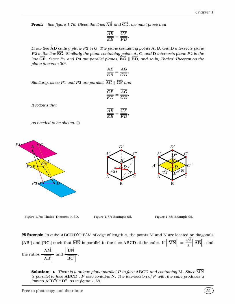
Chapter 1
Proof: See figure 1.76. Given the lines←→AB and
←→CD, we must prove that
AE
EB=
CF
FD.
Draw line←→AD cutting plane P2 in G. The plane containing points A, B, and D intersects plane
P2 in the line←→EG. Similarly the plane containing points A, C, and D intersects plane P2 in the
line←→GF. Since P2 and P3 are parallel planes,
←→EG ‖ ←→BD, and so by Thales’ Theorem on the
plane (theorem 30),
AE
EB=
AG
GD.
Similarly, since P1 and P2 are parallel,←→AC ‖ ←→GF and
CF
FD=
AG
GD.
It follows that
AE
EB=
CF
FD,
as needed to be shewn.
bA
bE bG
b C
bB b D
bF
P1
P2
P3
Figure 1.76: Thales’ Theorem in 3D.
b
Mb
Nb
Ab
B
b
C
b D
bA′
bB′
bC′
bD′
Figure 1.77: Example 95.
bA′′
bB′′
b C′′
bD′′
b
M
b
Nb
Ab
B
b
C
b D
bA′
bB′
bC′
bD′
Figure 1.78: Example 95.
95 Example In cube ABCDD′C′B′A′ of edge of length a, the points M and N are located on diagonals
[AB′] and [BC′] such that−−→MN is parallel to the face ABCD of the cube. If
−−→MN =
√5
3
−→AB, find
the ratios
−−→AM−−→AB′ and
−→BN−−→BC′ .
Solution: I There is a unique plane parallel P to face ABCD and containing M. Since−−→MN
is parallel to face ABCD , P also contains N. The intersection of P with the cube produces a
lamina A′′B′′C′′D′′, as in figure 1.78.
Free to photocopy and distribute 51
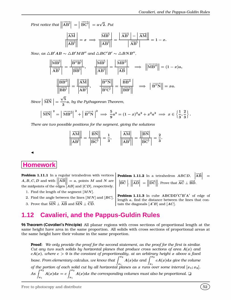
Cavalieri, and the Pappus-Guldin Rules
First notice that−−→AB′
= −−→BC′ = a
√2. Put−−→AM
−−→AB′ = x =⇒
−−→MB′−−→AB′ =
−−→AB′− −−→AM
−−→AB′ = 1− x.
Now, as 4B′AB ∼ 4B′MB′′ and 4BC′B′ ∼ 4BNB′′,−−→MB′−−→AB′ =
−−−→B′′B′−−→BB′ ,
−−→MB′−−→AB′ =
−−−→MB′′−→AB =⇒
−−−→MB′′ = (1− x)a,−−→BB′′
−−→BB′ =
−−→AM−−→AB′ , −−→B′′N
−−→B′C′ =
−−→BB′′−−→BB′ =⇒
−−→B′′N = xa.
Since−−→MN
= √5
3a, by the Pythagorean Theorem,−−→MN
2 =−−−→MB′′
2 +−−→B′′N
2 =⇒ 5
9a2 = (1 − x)2a2 + x2a2 =⇒ x ∈
§1
3,2
3
ª.
There are two possible positions for the segment, giving the solutions−−→AM−−→AB′ =
−→BN−−→BC′ =
1
3,
−−→AM−−→AB′ =
−→BN−−→BC′ =
2
3.
J
HomeworkProblem 1.11.1 In a regular tetrahedron with vertices
A, B, C, D and with
−→AB = a, points M and N are
the midpoints of the edges [AB] and [CD], respectively.
1. Find the length of the segment [MN ].
2. Find the angle between the lines [MN ] and [BC].
3. Prove that−−→MN ⊥ −→AB and
−−→MN ⊥ −→CD.
Problem 1.11.2 In a tetrahedron ABCD,
−→AB
=−→BC, −→AD
= −→DC. Prove that
−→AC ⊥ −→BD.
Problem 1.11.3 In cube ABCDD′C′B′A′ of edge of
length a, find the distance between the lines that con-tain the diagonals [A′B] and [AC].
1.12 Cavalieri, and the Pappus-Guldin Rules96 Theorem (Cavalieri’s Principle) All planar regions with cross sections of proportional length at thesame height have area in the same proportion. All solids with cross sections of proportional areas atthe same height have their volume in the same proportion.
Proof: We only provide the proof for the second statement, as the proof for the first is similar.
Cut any two such solids by horizontal planes that produce cross sections of area A(x) and
cA(x), where c > 0 is the constant of proportionality, at an arbitrary height x above a fixed
base. From elementary calculus, we know that
Z x2
x1
A(x)dx and
Z x2
x1
cA(x)dx give the volume
of the portion of each solid cut by all horizontal planes as x runs over some interval [x1; x2].
As
Z x2
x1
A(x)dx = c
Z x2
x1
A(x)dx the corresponding volumes must also be proportional.
Free to photocopy and distribute 52
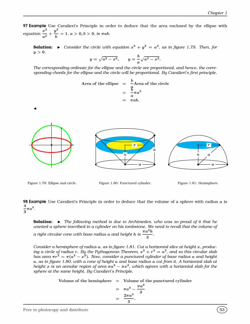
Chapter 1
97 Example Use Cavalieri’s Principle in order to deduce that the area enclosed by the ellipse with
equationx2
a2+
y2
b= 1, a > 0, b > 0, is πab.
Solution: I Consider the circle with equation x2 + y2 = a2, as in figure 1.79. Then, for
y > 0,
y =p
a2 − x2, y =b
a
pa2 − x2.
The corresponding ordinate for the ellipse and the circle are proportional, and hence, the corre-
sponding chords for the ellipse and the circle will be proportional. By Cavalieri’s first principle,
Area of the ellipse =b
aArea of the circle
=b
aπa2
= πab.
J
b b
b
b
Figure 1.79: Ellipse and circle.
b
b b
b b
b b
a
x
x
a
Figure 1.80: Punctured cylinder.
bb b
b b
x
a
r
a
Figure 1.81: Hemisphere.
98 Example Use Cavalieri’s Principle in order to deduce that the volume of a sphere with radius a is4
3πa3.
Solution: I The following method is due to Archimedes, who was so proud of it that he
wanted a sphere inscribed in a cylinder on his tombstone. We need to recall that the volume of
a right circular cone with base radius a and height h isπa2h
3.
Consider a hemisphere of radius a, as in figure 1.81. Cut a horizontal slice at height x, produc-
ing a circle of radius r. By the Pythagorean Theorem, x2 + r2 = a2, and so this circular slab
has area πr2 = π(a2 − x2). Now, consider a punctured cylinder of base radius a and height
a, as in figure 1.80, with a cone of height a and base radius a cut from it. A horizontal slab at
height x is an annular region of area πa2 − πx2, which agrees with a horizontal slab for the
sphere at the same height. By Cavalieri’s Principle,
Volume of the hemisphere = Volume of the punctured cylinder
= πa3 − πa3
3
=2πa3
3.
Free to photocopy and distribute 53
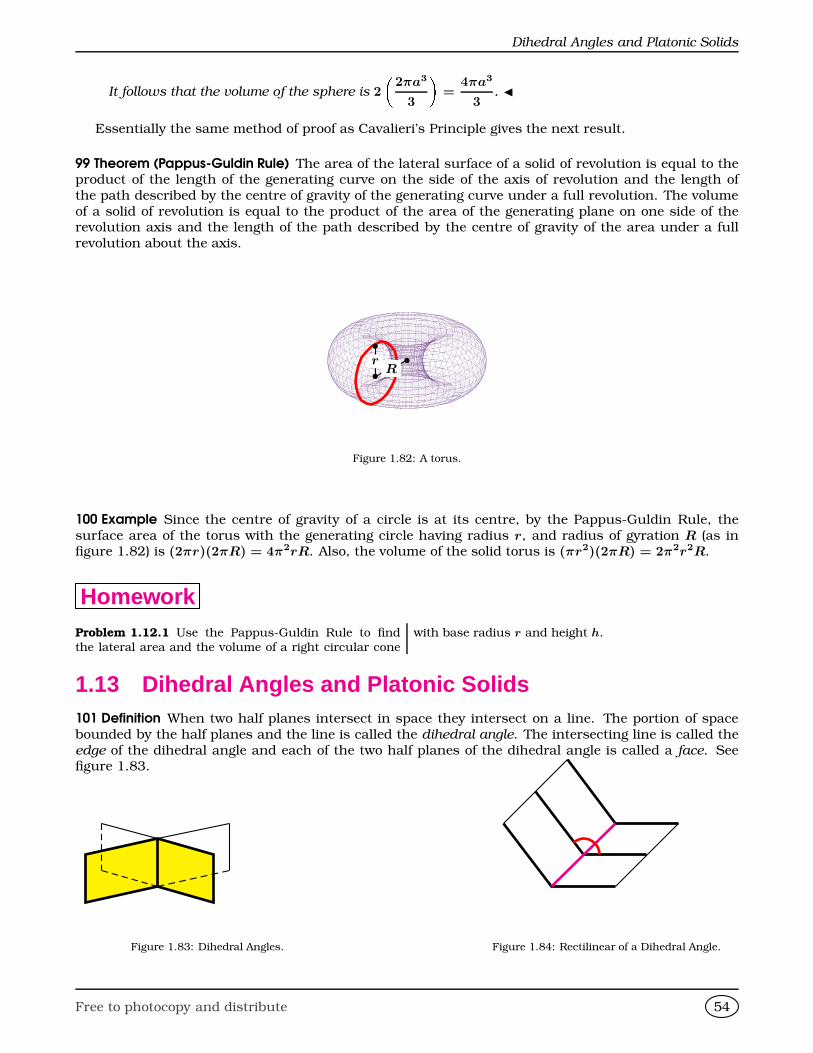
Dihedral Angles and Platonic Solids
It follows that the volume of the sphere is 2
2πa3
3
=
4πa3
3. J
Essentially the same method of proof as Cavalieri’s Principle gives the next result.
99 Theorem (Pappus-Guldin Rule) The area of the lateral surface of a solid of revolution is equal to theproduct of the length of the generating curve on the side of the axis of revolution and the length ofthe path described by the centre of gravity of the generating curve under a full revolution. The volumeof a solid of revolution is equal to the product of the area of the generating plane on one side of therevolution axis and the length of the path described by the centre of gravity of the area under a fullrevolution about the axis.
b
b
b
Rr
Figure 1.82: A torus.
100 Example Since the centre of gravity of a circle is at its centre, by the Pappus-Guldin Rule, thesurface area of the torus with the generating circle having radius r, and radius of gyration R (as infigure 1.82) is (2πr)(2πR) = 4π2rR. Also, the volume of the solid torus is (πr2)(2πR) = 2π2r2R.
HomeworkProblem 1.12.1 Use the Pappus-Guldin Rule to findthe lateral area and the volume of a right circular cone
with base radius r and height h.
1.13 Dihedral Angles and Platonic Solids101 Definition When two half planes intersect in space they intersect on a line. The portion of spacebounded by the half planes and the line is called the dihedral angle. The intersecting line is called theedge of the dihedral angle and each of the two half planes of the dihedral angle is called a face. Seefigure 1.83.
Figure 1.83: Dihedral Angles. Figure 1.84: Rectilinear of a Dihedral Angle.
Free to photocopy and distribute 54
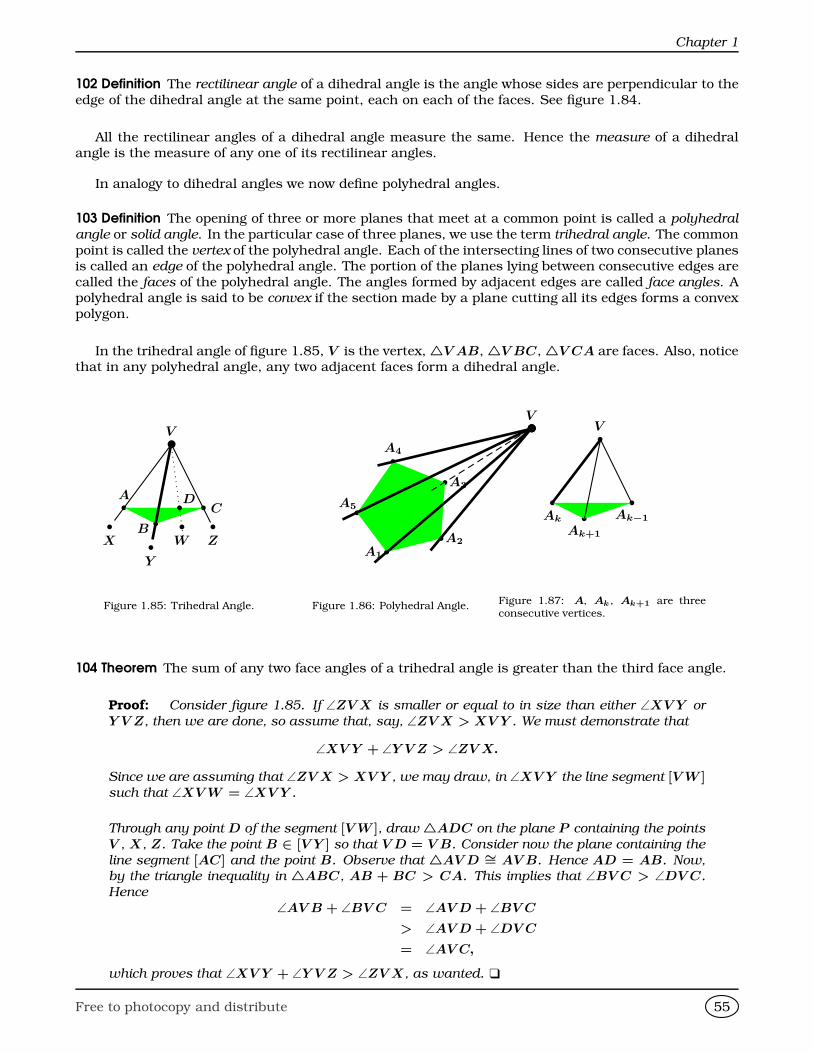
Chapter 1
102 Definition The rectilinear angle of a dihedral angle is the angle whose sides are perpendicular to theedge of the dihedral angle at the same point, each on each of the faces. See figure 1.84.
All the rectilinear angles of a dihedral angle measure the same. Hence the measure of a dihedralangle is the measure of any one of its rectilinear angles.
In analogy to dihedral angles we now define polyhedral angles.
103 Definition The opening of three or more planes that meet at a common point is called a polyhedral
angle or solid angle. In the particular case of three planes, we use the term trihedral angle. The commonpoint is called the vertex of the polyhedral angle. Each of the intersecting lines of two consecutive planesis called an edge of the polyhedral angle. The portion of the planes lying between consecutive edges arecalled the faces of the polyhedral angle. The angles formed by adjacent edges are called face angles. Apolyhedral angle is said to be convex if the section made by a plane cutting all its edges forms a convexpolygon.
In the trihedral angle of figure 1.85, V is the vertex,4V AB,4V BC,4V CA are faces. Also, noticethat in any polyhedral angle, any two adjacent faces form a dihedral angle.
bV
bA
b Cb
B
bD
b
X b
Y
b
Z
b
W
Figure 1.85: Trihedral Angle.
bV
bP
bA1
b A2
b A3
b
A4
bA5
Figure 1.86: Polyhedral Angle.
bV
b
Ak
b
Ak−1b
Ak+1
Figure 1.87: A, Ak , Ak+1 are threeconsecutive vertices.
104 Theorem The sum of any two face angles of a trihedral angle is greater than the third face angle.
Proof: Consider figure 1.85. If ∠ZV X is smaller or equal to in size than either ∠XV Y or
Y V Z, then we are done, so assume that, say, ∠ZV X > XV Y . We must demonstrate that
∠XV Y + ∠Y V Z > ∠ZV X.
Since we are assuming that ∠ZV X > XV Y , we may draw, in ∠XV Y the line segment [V W ]such that ∠XV W = ∠XV Y .
Through any point D of the segment [V W ], draw4ADC on the plane P containing the points
V , X, Z. Take the point B ∈ [V Y ] so that V D = V B. Consider now the plane containing the
line segment [AC] and the point B. Observe that 4AV D ∼= AV B. Hence AD = AB. Now,
by the triangle inequality in 4ABC, AB + BC > CA. This implies that ∠BV C > ∠DV C.
Hence
∠AV B + ∠BV C = ∠AV D + ∠BV C
> ∠AV D + ∠DV C
= ∠AV C,
which proves that ∠XV Y + ∠Y V Z > ∠ZV X, as wanted.
Free to photocopy and distribute 55
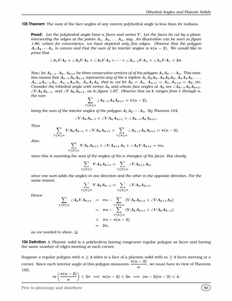
Dihedral Angles and Platonic Solids
105 Theorem The sum of the face angles of any convex polyhedral angle is less than 2π radians.
Proof: Let the polyhedral angle have n faces and vertex V . Let the faces be cut by a plane,
intersecting the edges at the points A1, A2, . . . An, say. An illustration can be seen in figure
1.86, where for convenience, we have depicted only five edges. Observe that the polygon
A1A2 · · ·An is convex and that the sum of its interior angles is π(n − 2). We would like to
prove that
∠A1V A2 + ∠A2V A3 + ∠A3V A4 + · · ·+ ∠An−1V An + ∠AnV A1 < 2π.
Now, let Ak−1, Ak, Ak+1 be three consecutive vertices of of the polygon A1A2 · · ·An. This nota-
tion means that Ak−1AkAk+1 represents any of the n triplets A1A2A3, A2A3A4, A3A4A5, . . . ,
An−2An−1An, An−1AnA1, AnA1A2, that is, we let A0 = An, An+1 = A1, An+2 = A2, etc.
Consider the trihedral angle with vertex Ak and whose face angles at Ak are ∠Ak−1AkAk+1,
∠V AkAk−1, and ∠V AkAk+1, as in figure 1.87. Observe that as k ranges from 1 through n,
the sum X1≤k≤n
∠Ak−1AkAk+1 = π(n− 2),
being the sum of the interior angles of the polygon A1A2 · · ·An. By Theorem 104,
∠V AkAk−1 + ∠V AkAk+1 > ∠Ak−1AkAk+1.
Thus X1≤k≤n
V AkAk−1 + ∠V AkAk+1 >X
1≤k≤n
∠Ak−1AkAk+1 = π(n− 2).
Also, X1≤k≤n
V AkAk+1 + ∠V Ak+1Ak + ∠AkV Ak+1 = πn,
since this is summing the sum of the angles of the n triangles of the faces. But clearlyX1≤k≤n
V AkAk+1 =X
1≤k≤n
∠V Ak+1Ak,
since one sum adds the angles in one direction and the other in the opposite direction. For the
same reason, X1≤k≤n
V AkAk−1 =X
1≤k≤n
∠V AkAk+1.
Hence X1≤k≤n
∠AkV Ak+1 = πn−X
1≤k≤n
(V AkAk+1 + ∠V Ak+1Ak)
= πn−X
1≤k≤n
(V AkAk+1 + ∠V AkAk−1)
< πn− π(n− 2)
= 2π,
as we needed to shew.
106 Definition A Platonic solid is a polyhedron having congruent regular polygon as faces and havingthe same number of edges meeting at each corner.
Suppose a regular polygon with n ≥ 3 sides is a face of a platonic solid with m ≥ 3 faces meeting at a
corner. Since each interior angle of this polygon measuresπ(n− 2)
n, we must have in view of Theorem
105,
m
π(n− 2)
n
< 2π =⇒ m(n− 2) < 2n =⇒ (m− 2)(n− 2) < 4.
Free to photocopy and distribute 56
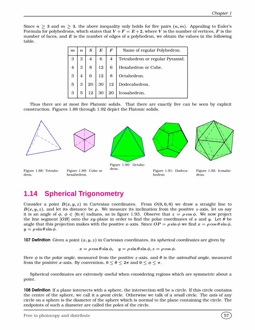
Chapter 1
Since n ≥ 3 and m ≥ 3, the above inequality only holds for five pairs (n, m). Appealing to Euler’sFormula for polyhedrons, which states that V +F = E +2, where V is the number of vertices, F is thenumber of faces, and E is the number of edges of a polyhedron, we obtain the values in the followingtable.
m n S E F Name of regular Polyhedron.
3 3 4 6 4 Tetrahedron or regular Pyramid.
4 3 8 12 6 Hexahedron or Cube.
3 4 6 12 8 Octahedron.
5 3 20 30 12 Dodecahedron.
3 5 12 30 20 Icosahedron.
Thus there are at most five Platonic solids. That there are exactly five can be seen by explicitconstruction. Figures 1.88 through 1.92 depict the Platonic solids.
Figure 1.88: Tetrahe-dron.
Figure 1.89: Cube orhexahedron.
Figure 1.90: Octahe-dron.
Figure 1.91: Dodeca-hedron
Figure 1.92: Icosahe-dron.
1.14 Spherical TrigonometryConsider a point B(x, y, z) in Cartesian coordinates. From O(0, 0, 0) we draw a straight line toB(x, y, z), and let its distance be ρ. We measure its inclination from the positive z-axis, let us sayit is an angle of φ, φ ∈ [0;π] radians, as in figure 1.93. Observe that z = ρ cos φ. We now projectthe line segment [OB] onto the xy-plane in order to find the polar coordinates of x and y. Let θ beangle that this projection makes with the positive x-axis. Since OP = ρ sin φ we find x = ρ cos θ sin φ,y = ρ sin θ sin φ.
107 Definition Given a point (x, y, z) in Cartesian coordinates, its spherical coordinates are given by
x = ρ cos θ sin φ, y = ρ sin θ sin φ, z = ρ cos φ.
Here φ is the polar angle, measured from the positive z-axis, and θ is the azimuthal angle, measuredfrom the positive x-axis. By convention, 0 ≤ θ ≤ 2π and 0 ≤ φ ≤ π.
Spherical coordinates are extremely useful when considering regions which are symmetric about apoint.
108 Definition If a plane intersects with a sphere, the intersection will be a circle. If this circle containsthe centre of the sphere, we call it a great circle. Otherwise we talk of a small circle. The axis of anycircle on a sphere is the diameter of the sphere which is normal to the plane containing the circle. Theendpoints of such a diameter are called the poles of the circle.
Free to photocopy and distribute 57
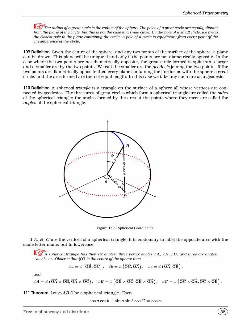
Spherical Trigonometry
The radius of a great circle is the radius of the sphere. The poles of a great circle are equally distant
from the plane of the circle, but this is not the case in a small circle. By the pole of a small circle, we mean
the closest pole to the plane containing the circle. A pole of a circle is equidistant from every point of the
circumference of the circle.
109 Definition Given the centre of the sphere, and any two points of the surface of the sphere, a planecan be drawn. This plane will be unique if and only if the points are not diametrically opposite. In thecase where the two points are not diametrically opposite, the great circle formed is split into a largerand a smaller arc by the two points. We call the smaller arc the geodesic joining the two points. If thetwo points are diametrically opposite then every plane containing the line forms with the sphere a greatcircle, and the arcs formed are then of equal length. In this case we take any such arc as a geodesic.
110 Definition A spherical triangle is a triangle on the surface of a sphere all whose vertices are con-nected by geodesics. The three arcs of great circles which form a spherical triangle are called the sides
of the spherical triangle; the angles formed by the arcs at the points where they meet are called theangles of the spherical triangle.
b B
b
P
φ
θ
ρ
ρsin
φ
ρcosφ
Figure 1.93: Spherical Coordinates.
If A, B, C are the vertices of a spherical triangle, it is customary to label the opposite arcs with thesame letter name, but in lowercase.
A spherical triangle has then six angles: three vertex angles ∠A, ∠B, ∠C , and three arc angles,
∠a, ∠b, ∠c. Observe that if O is the centre of the sphere then
∠a = ∠
−→OB,−→OC
, ∠b = ∠
−→OC,−→OA
, ∠c = ∠
−→OA,−→OB
,
and
∠A = ∠
−→OA× −→OB,
−→OA × −→OC
, ∠B = ∠
−→OB × −→OC,
−→OB × −→OA
, ∠C = ∠
−→OC × −→OA,
−→OC × −→OB
.
111 Theorem Let 4ABC be a spherical triangle. Then
cos a cos b + sin a sin b cos C = cos c.
Free to photocopy and distribute 58
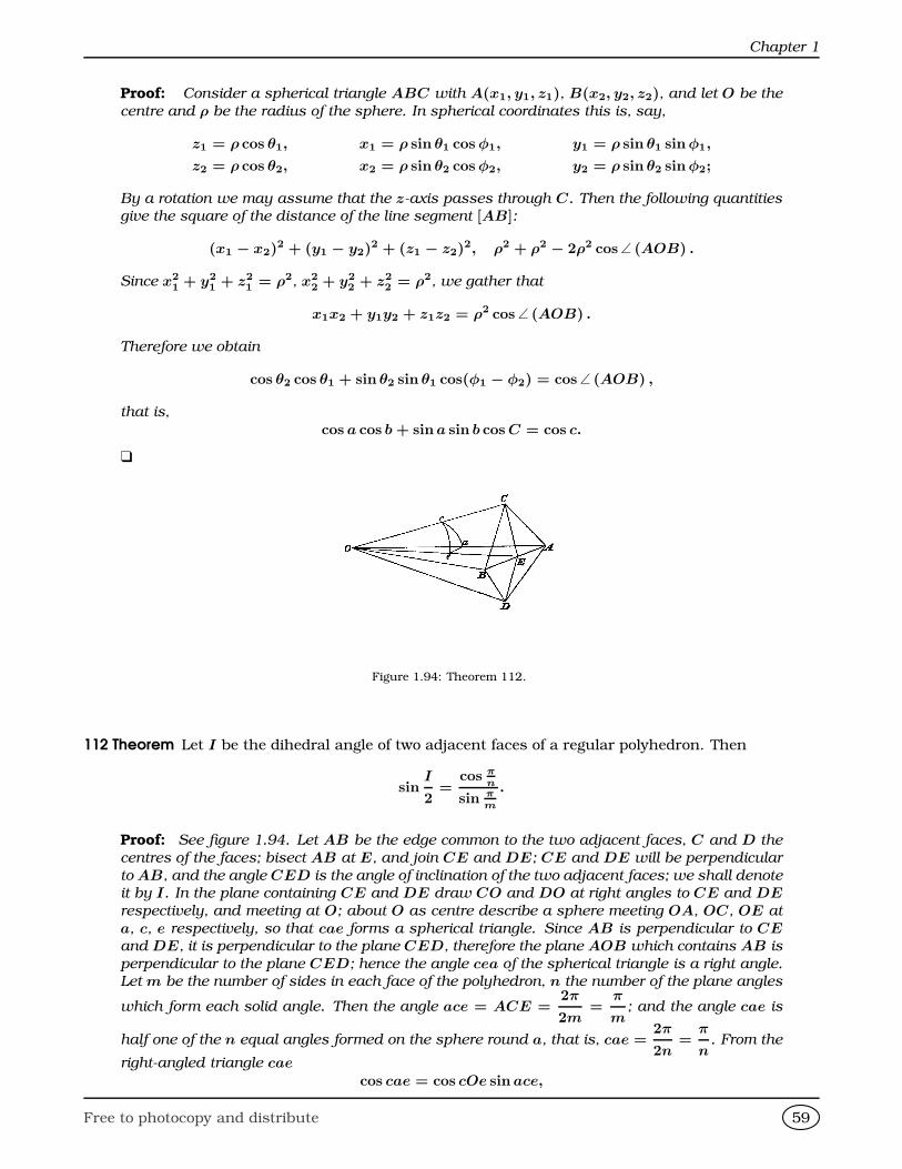
Chapter 1
Proof: Consider a spherical triangle ABC with A(x1, y1, z1), B(x2, y2, z2), and let O be the
centre and ρ be the radius of the sphere. In spherical coordinates this is, say,
z1 = ρ cos θ1, x1 = ρ sin θ1 cos φ1, y1 = ρ sin θ1 sin φ1,
z2 = ρ cos θ2, x2 = ρ sin θ2 cos φ2, y2 = ρ sin θ2 sin φ2;
By a rotation we may assume that the z-axis passes through C. Then the following quantities
give the square of the distance of the line segment [AB]:
(x1 − x2)2 + (y1 − y2)
2 + (z1 − z2)2, ρ2 + ρ2 − 2ρ2 cos ∠ (AOB) .
Since x21 + y2
1 + z21 = ρ2, x2
2 + y22 + z2
2 = ρ2, we gather that
x1x2 + y1y2 + z1z2 = ρ2 cos ∠ (AOB) .
Therefore we obtain
cos θ2 cos θ1 + sin θ2 sin θ1 cos(φ1 − φ2) = cos ∠ (AOB) ,
that is,
cos a cos b + sin a sin b cos C = cos c.
Figure 1.94: Theorem 112.
112 Theorem Let I be the dihedral angle of two adjacent faces of a regular polyhedron. Then
sinI
2=
cos πn
sin πm
.
Proof: See figure 1.94. Let AB be the edge common to the two adjacent faces, C and D the
centres of the faces; bisect AB at E, and join CE and DE; CE and DE will be perpendicular
to AB, and the angle CED is the angle of inclination of the two adjacent faces; we shall denote
it by I. In the plane containing CE and DE draw CO and DO at right angles to CE and DErespectively, and meeting at O; about O as centre describe a sphere meeting OA, OC, OE at
a, c, e respectively, so that cae forms a spherical triangle. Since AB is perpendicular to CEand DE, it is perpendicular to the plane CED, therefore the plane AOB which contains AB is
perpendicular to the plane CED; hence the angle cea of the spherical triangle is a right angle.
Let m be the number of sides in each face of the polyhedron, n the number of the plane angles
which form each solid angle. Then the angle ace = ACE =2π
2m=
π
m; and the angle cae is
half one of the n equal angles formed on the sphere round a, that is, cae =2π
2n=
π
n. From the
right-angled triangle caecos cae = cos cOe sin ace,
Free to photocopy and distribute 59
Spherical Trigonometry
that is cosπ
n= cos
π
2− I
2
sin
π
m;
therefore sinI
2=
cosπ
n
sinπ
m
.
113 Theorem Let r and R be, respectively, the radii of the inscribed and circumscribed spheres of aregular polyhedron. Then
r =a
2cot
π
mtan
I
2, R =
a
2tan
I
2tan
π
n.
Here a is the length of any edge of the polyhedron, and I is the dihedral angle of any two faces.
Proof: Let the edge AB = a, let OC = r and OA = R, so that r is the radius of the inscribed
sphere, and R is the radius of the circumscribed sphere. Then
CE = AE cot ACE =a
2cot
π
m,
r = CE tan CEO = CE tanI
2=
a
2cot
π
mtan
I
2;
also r = R cos aOc = R cot eca cot eac = R cotπ
mcot
π
n;
therefore R = r tanπ
mtan
π
n=
a
2tan
I
2tan
π
n.
From the above formulæ we now easily find that the volume of the pyramid which has one face of the
polyhedron for base and O for vertex isr
3
ma2
4cot
π
m, and therefore the volume of the polyhedron is
mFra2
12cot
π
m.
Furthermore, the area of one face of the polyhedron isma2
4cot
π
m, and therefore the surface area of
the polyhedron ismFa2
4cot
π
m.
HomeworkProblem 1.14.1 The four vertices of a regular tetrahe-dron are
V1 =
1
0
0
DZ, V2 =
−1/2√
3/2
0
DZ,
V3 =
−1/2
−√
3/2
0
DZ, V4 =
0
0√2
DZ.
What is the cosine of the dihedral angle between any
pair of faces of the tetrahedron?
Problem 1.14.2 Consider a tetrahedron whose edge
measures a. Shew that its volume isa3√
2
12, its sur-
face area is a2√
3, and that the radius of the inscribed
sphere isa√
6
12.
Problem 1.14.3 Consider a cube whose edge measures
a. Shew that its volume is a3, its surface area is 6a2,and that the radius of the inscribed sphere is
a
2.
Problem 1.14.4 Consider an octahedron whose edge
Free to photocopy and distribute 60
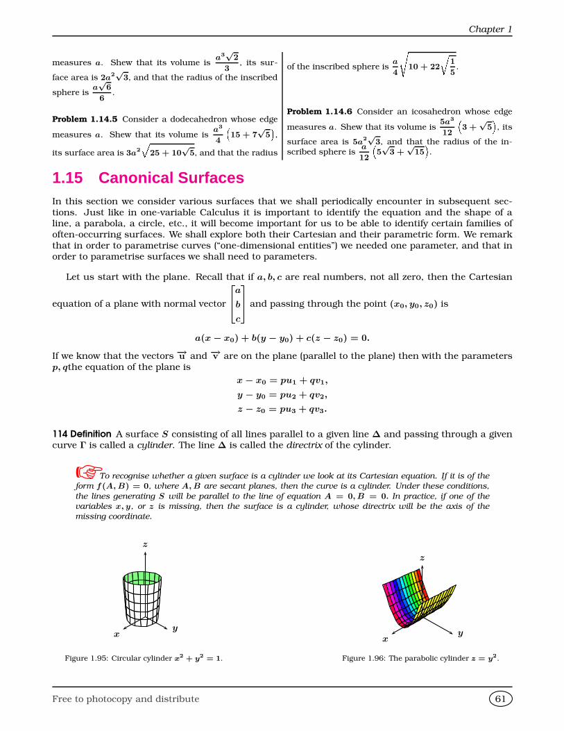
Chapter 1
measures a. Shew that its volume isa3√
2
3, its sur-
face area is 2a2√
3, and that the radius of the inscribed
sphere isa√
6
6.
Problem 1.14.5 Consider a dodecahedron whose edge
measures a. Shew that its volume isa3
4
15 + 7
√5,
its surface area is 3a2
È25 + 10
√5, and that the radius
of the inscribed sphere isa
4
Ê10 + 22
É1
5.
Problem 1.14.6 Consider an icosahedron whose edge
measures a. Shew that its volume is5a3
12
3 +√
5, its
surface area is 5a2√
3, and that the radius of the in-scribed sphere is
a
12
5√
3 +√
15.
1.15 Canonical SurfacesIn this section we consider various surfaces that we shall periodically encounter in subsequent sec-tions. Just like in one-variable Calculus it is important to identify the equation and the shape of aline, a parabola, a circle, etc., it will become important for us to be able to identify certain families ofoften-occurring surfaces. We shall explore both their Cartesian and their parametric form. We remarkthat in order to parametrise curves (“one-dimensional entities”) we needed one parameter, and that inorder to parametrise surfaces we shall need to parameters.
Let us start with the plane. Recall that if a, b, c are real numbers, not all zero, then the Cartesian
equation of a plane with normal vector
264a
b
c
375 and passing through the point (x0, y0, z0) is
a(x− x0) + b(y − y0) + c(z − z0) = 0.
If we know that the vectors −→u and −→v are on the plane (parallel to the plane) then with the parametersp, qthe equation of the plane is
x− x0 = pu1 + qv1,
y − y0 = pu2 + qv2,
z − z0 = pu3 + qv3.
114 Definition A surface S consisting of all lines parallel to a given line ∆ and passing through a givencurve Γ is called a cylinder. The line ∆ is called the directrix of the cylinder.
To recognise whether a given surface is a cylinder we look at its Cartesian equation. If it is of the
form f(A, B) = 0, where A, B are secant planes, then the curve is a cylinder. Under these conditions,
the lines generating S will be parallel to the line of equation A = 0, B = 0. In practice, if one of the
variables x, y, or z is missing, then the surface is a cylinder, whose directrix will be the axis of the
missing coordinate.
xy
z
Figure 1.95: Circular cylinder x2 + y2 = 1.
xy
z
Figure 1.96: The parabolic cylinder z = y2.
Free to photocopy and distribute 61
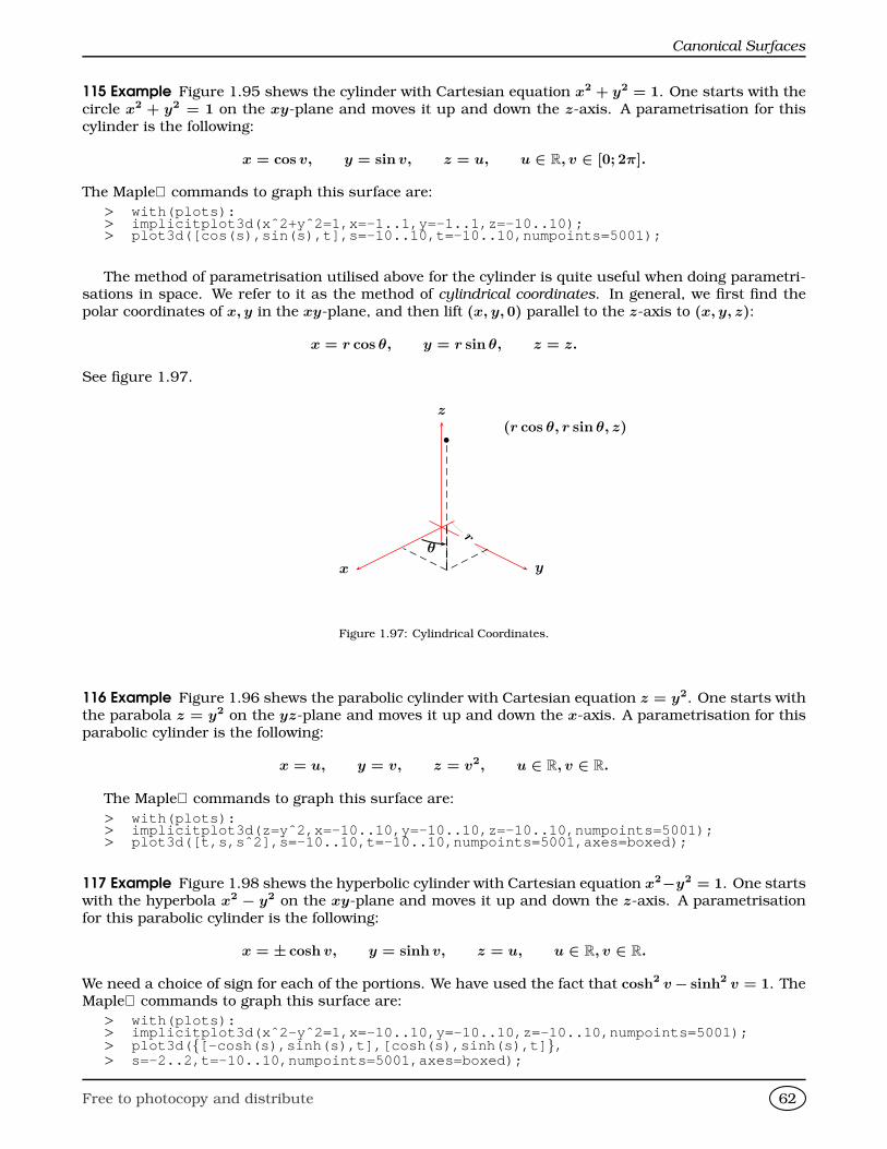
Canonical Surfaces
115 Example Figure 1.95 shews the cylinder with Cartesian equation x2 + y2 = 1. One starts with thecircle x2 + y2 = 1 on the xy-plane and moves it up and down the z-axis. A parametrisation for thiscylinder is the following:
x = cos v, y = sin v, z = u, u ∈ R, v ∈ [0; 2π].
The Maple commands to graph this surface are:
> with(plots):> implicitplot3d(xˆ2+yˆ2=1,x=-1..1,y=-1..1,z=-10..10) ;> plot3d([cos(s),sin(s),t],s=-10..10,t=-10..10,numpoi nts=5001);
The method of parametrisation utilised above for the cylinder is quite useful when doing parametri-sations in space. We refer to it as the method of cylindrical coordinates. In general, we first find thepolar coordinates of x, y in the xy-plane, and then lift (x, y, 0) parallel to the z-axis to (x, y, z):
x = r cos θ, y = r sin θ, z = z.
See figure 1.97.
x y
z
b(r cos θ, r sin θ, z)
θr
Figure 1.97: Cylindrical Coordinates.
116 Example Figure 1.96 shews the parabolic cylinder with Cartesian equation z = y2. One starts withthe parabola z = y2 on the yz-plane and moves it up and down the x-axis. A parametrisation for thisparabolic cylinder is the following:
x = u, y = v, z = v2, u ∈ R, v ∈ R.
The Maple commands to graph this surface are:
> with(plots):> implicitplot3d(z=yˆ2,x=-10..10,y=-10..10,z=-10..10, numpoints=5001);> plot3d([t,s,sˆ2],s=-10..10,t=-10..10,numpoints=5001 ,axes=boxed);
117 Example Figure 1.98 shews the hyperbolic cylinder with Cartesian equation x2−y2 = 1. One startswith the hyperbola x2 − y2 on the xy-plane and moves it up and down the z-axis. A parametrisationfor this parabolic cylinder is the following:
x = ± cosh v, y = sinh v, z = u, u ∈ R, v ∈ R.
We need a choice of sign for each of the portions. We have used the fact that cosh2 v− sinh2 v = 1. TheMaple commands to graph this surface are:
> with(plots):> implicitplot3d(xˆ2-yˆ2=1,x=-10..10,y=-10..10,z=-10. .10,numpoints=5001);> plot3d( [-cosh(s),sinh(s),t],[cosh(s),sinh(s),t] ,> s=-2..2,t=-10..10,numpoints=5001,axes=boxed);
Free to photocopy and distribute 62
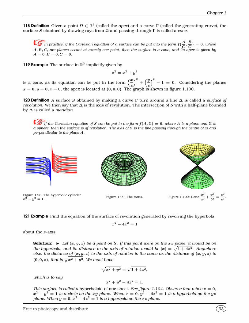
Chapter 1
118 Definition Given a point Ω ∈ R3 (called the apex) and a curve Γ (called the generating curve), the
surface S obtained by drawing rays from Ω and passing through Γ is called a cone.
In practice, if the Cartesian equation of a surface can be put into the form f(A
C,B
C) = 0, where
A, B, C, are planes secant at exactly one point, then the surface is a cone, and its apex is given by
A = 0, B = 0, C = 0.
119 Example The surface in R3 implicitly given by
z2 = x2 + y2
is a cone, as its equation can be put in the formx
z
2
+y
z
2
− 1 = 0. Considering the planes
x = 0, y = 0, z = 0, the apex is located at (0, 0, 0). The graph is shewn in figure 1.100.
120 Definition A surface S obtained by making a curve Γ turn around a line ∆ is called a surface of
revolution. We then say that ∆ is the axis of revolution. The intersection of S with a half-plane boundedby ∆ is called a meridian.
If the Cartesian equation of S can be put in the form f(A, Σ) = 0, where A is a plane and Σ is
a sphere, then the surface is of revolution. The axis of S is the line passing through the centre of Σ and
perpendicular to the plane A.
Figure 1.98: The hyperbolic cylinderx2 − y2 = 1.
Figure 1.99: The torus. Figure 1.100: Conex2
a2+
y2
b2=
z2
c2.
121 Example Find the equation of the surface of revolution generated by revolving the hyperbola
x2 − 4z2 = 1
about the z-axis.
Solution: I Let (x, y, z) be a point on S. If this point were on the xz plane, it would be on
the hyperbola, and its distance to the axis of rotation would be |x| =p
1 + 4z2. Anywhere
else, the distance of (x, y, z) to the axis of rotation is the same as the distance of (x, y, z) to
(0, 0, z), that isÈ
x2 + y2. We must haveÈx2 + y2 =
p1 + 4z2,
which is to say
x2 + y2 − 4z2 = 1.
This surface is called a hyperboloid of one sheet. See figure 1.104. Observe that when z = 0,
x2 + y2 = 1 is a circle on the xy plane. When x = 0, y2 − 4z2 = 1 is a hyperbola on the yzplane. When y = 0, x2 − 4z2 = 1 is a hyperbola on the xz plane.
Free to photocopy and distribute 63
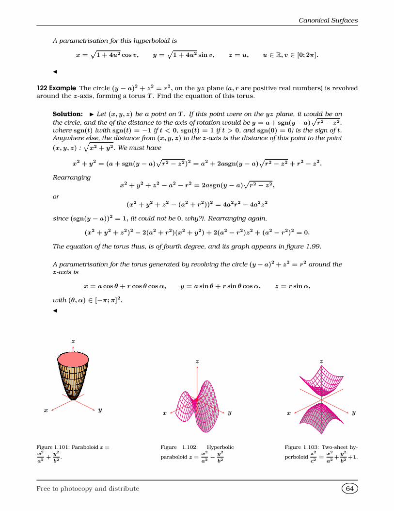
Canonical Surfaces
A parametrisation for this hyperboloid is
x =p
1 + 4u2 cos v, y =p
1 + 4u2 sin v, z = u, u ∈ R, v ∈ [0; 2π].
J
122 Example The circle (y − a)2 + z2 = r2, on the yz plane (a, r are positive real numbers) is revolvedaround the z-axis, forming a torus T . Find the equation of this torus.
Solution: I Let (x, y, z) be a point on T . If this point were on the yz plane, it would be on
the circle, and the of the distance to the axis of rotation would be y = a +sgn(y− a)p
r2 − z2,
where sgn(t) (with sgn(t) = −1 if t < 0, sgn(t) = 1 if t > 0, and sgn(0) = 0) is the sign of t.Anywhere else, the distance from (x, y, z) to the z-axis is the distance of this point to the point
(x, y, z) :È
x2 + y2. We must have
x2 + y2 = (a + sgn(y − a)p
r2 − z2)2 = a2 + 2asgn(y − a)p
r2 − z2 + r2 − z2.
Rearranging
x2 + y2 + z2 − a2 − r2 = 2asgn(y − a)p
r2 − z2,
or
(x2 + y2 + z2 − (a2 + r2))2 = 4a2r2 − 4a2z2
since (sgn(y − a))2 = 1, (it could not be 0, why?). Rearranging again,
(x2 + y2 + z2)2 − 2(a2 + r2)(x2 + y2) + 2(a2 − r2)z2 + (a2 − r2)2 = 0.
The equation of the torus thus, is of fourth degree, and its graph appears in figure 1.99.
A parametrisation for the torus generated by revolving the circle (y− a)2 + z2 = r2 around the
z-axis is
x = a cos θ + r cos θ cos α, y = a sin θ + r sin θ cos α, z = r sin α,
with (θ, α) ∈ [−π; π]2.
J
x y
z
Figure 1.101: Paraboloid z =x2
a2+
y2
b2.
x y
z
Figure 1.102: Hyperbolic
paraboloid z =x2
a2− y2
b2
x y
z
Figure 1.103: Two-sheet hy-
perboloidz2
c2=
x2
a2+
y2
b2+1.
Free to photocopy and distribute 64
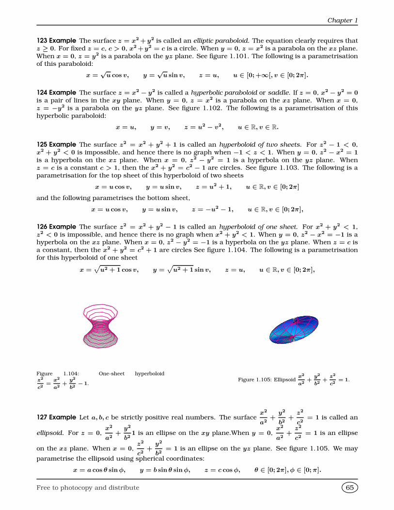
Chapter 1
123 Example The surface z = x2 +y2 is called an elliptic paraboloid. The equation clearly requires thatz ≥ 0. For fixed z = c, c > 0, x2 +y2 = c is a circle. When y = 0, z = x2 is a parabola on the xz plane.When x = 0, z = y2 is a parabola on the yz plane. See figure 1.101. The following is a parametrisationof this paraboloid:
x =√
u cos v, y =√
u sin v, z = u, u ∈ [0;+∞[, v ∈ [0; 2π].
124 Example The surface z = x2 − y2 is called a hyperbolic paraboloid or saddle. If z = 0, x2 − y2 = 0is a pair of lines in the xy plane. When y = 0, z = x2 is a parabola on the xz plane. When x = 0,z = −y2 is a parabola on the yz plane. See figure 1.102. The following is a parametrisation of thishyperbolic paraboloid:
x = u, y = v, z = u2 − v2, u ∈ R, v ∈ R.
125 Example The surface z2 = x2 + y2 + 1 is called an hyperboloid of two sheets. For z2 − 1 < 0,x2 + y2 < 0 is impossible, and hence there is no graph when −1 < z < 1. When y = 0, z2 − x2 = 1is a hyperbola on the xz plane. When x = 0, z2 − y2 = 1 is a hyperbola on the yz plane. Whenz = c is a constant c > 1, then the x2 + y2 = c2 − 1 are circles. See figure 1.103. The following is aparametrisation for the top sheet of this hyperboloid of two sheets
x = u cos v, y = u sin v, z = u2 + 1, u ∈ R, v ∈ [0; 2π]
and the following parametrises the bottom sheet,
x = u cos v, y = u sin v, z = −u2 − 1, u ∈ R, v ∈ [0; 2π],
126 Example The surface z2 = x2 + y2 − 1 is called an hyperboloid of one sheet. For x2 + y2 < 1,z2 < 0 is impossible, and hence there is no graph when x2 + y2 < 1. When y = 0, z2 − x2 = −1 is ahyperbola on the xz plane. When x = 0, z2 − y2 = −1 is a hyperbola on the yz plane. When z = c isa constant, then the x2 + y2 = c2 + 1 are circles See figure 1.104. The following is a parametrisationfor this hyperboloid of one sheet
x =p
u2 + 1 cos v, y =p
u2 + 1 sin v, z = u, u ∈ R, v ∈ [0; 2π],
Figure 1.104: One-sheet hyperboloidz2
c2=
x2
a2+
y2
b2− 1.
Figure 1.105: Ellipsoidx2
a2+
y2
b2+
z2
c2= 1.
127 Example Let a, b, c be strictly positive real numbers. The surfacex2
a2+
y2
b2+
z2
c2= 1 is called an
ellipsoid. For z = 0,x2
a2+
y2
b21 is an ellipse on the xy plane.When y = 0,
x2
a2+
z2
c2= 1 is an ellipse
on the xz plane. When x = 0,z2
c2+
y2
b2= 1 is an ellipse on the yz plane. See figure 1.105. We may
parametrise the ellipsoid using spherical coordinates:
x = a cos θ sin φ, y = b sin θ sin φ, z = c cos φ, θ ∈ [0; 2π], φ ∈ [0; π].
Free to photocopy and distribute 65
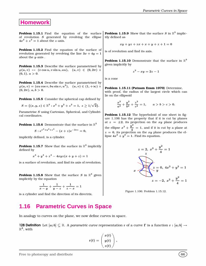
Parametric Curves in Space
Homework
Problem 1.15.1 Find the equation of the surfaceof revolution S generated by revolving the ellipse
4x2 + z2 = 1 about the z-axis.
Problem 1.15.2 Find the equation of the surface ofrevolution generated by revolving the line 3x + 4y = 1about the y-axis .
Problem 1.15.3 Describe the surface parametrised byϕ(u, v) 7→ (v cos u, v sin u, au), (u, v) ∈ (0, 2π) ×(0, 1), a > 0.
Problem 1.15.4 Describe the surface parametrised byϕ(u, v) = (au cos v, bu sin v, u2), (u, v) ∈ (1, +∞) ×(0, 2π), a, b > 0.
Problem 1.15.5 Consider the spherical cap defined by
S = (x, y, z) ∈ R3 : x2 + y2 + z2 = 1, z ≥ 1/
√2.
Parametrise S using Cartesian, Spherical, and Cylindri-cal coordinates.
Problem 1.15.6 Demonstrate that the surface in R3
S : ex2+y2+z2 − (x + z)e−2xz = 0,
implicitly defined, is a cylinder.
Problem 1.15.7 Shew that the surface in R3 implicitly
defined by
x4 + y4 + z4 − 4xyz(x + y + z) = 1
is a surface of revolution, and find its axis of revolution.
Problem 1.15.8 Shew that the surface S in R3 given
implicitly by the equation
1
x − y+
1
y − z+
1
z − x= 1
is a cylinder and find the direction of its directrix.
Problem 1.15.9 Shew that the surface S in R3 implic-
itly defined as
xy + yz + zx + x + y + z + 1 = 0
is of revolution and find its axis.
Problem 1.15.10 Demonstrate that the surface in R3
given implicitly by
z2 − xy = 2z − 1
is a cone
Problem 1.15.11 (Putnam Exam 1970) Determine,with proof, the radius of the largest circle which can
lie on the ellipsoid
x2
a2+
y2
b2+
z2
c2= 1, a > b > c > 0.
Problem 1.15.12 The hyperboloid of one sheet in fig-ure 1.106 has the property that if it is cut by planes
at z = ±2, its projection on the xy plane produces
the ellipse x2 +y2
4= 1, and if it is cut by a plane at
z = 0, its projection on the xy plane produces the el-lipse 4x2 + y2 = 1. Find its equation.
x y
z
z = −2, x2 +y2
4= 1
z = 2, x2 +y2
4= 1
z = 0, 4x2 + y2 = 1
Figure 1.106: Problem 1.15.12.
1.16 Parametric Curves in Space
In analogy to curves on the plane, we now define curves in space.
128 Definition Let [a; b] ⊆ R. A parametric curve representation r of a curve Γ is a function r : [a; b] →R
3, with
r(t) =
x(t)
y(t)
z(t)
,
Free to photocopy and distribute 66
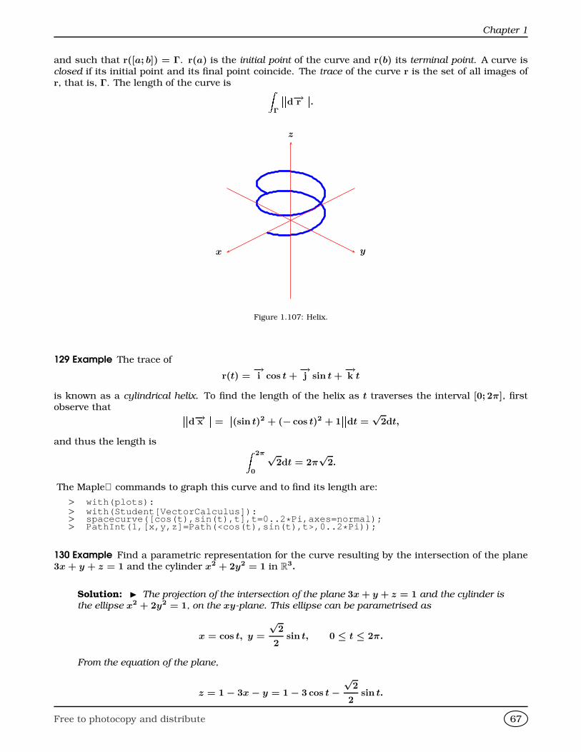
Chapter 1
and such that r([a; b]) = Γ. r(a) is the initial point of the curve and r(b) its terminal point. A curve isclosed if its initial point and its final point coincide. The trace of the curve r is the set of all images ofr, that is, Γ. The length of the curve is Z
Γ
d−→r .
x y
z
Figure 1.107: Helix.
129 Example The trace of
r(t) =−→i cos t +
−→j sin t +
−→k t
is known as a cylindrical helix. To find the length of the helix as t traverses the interval [0; 2π], firstobserve that d−→x = (sin t)2 + (− cos t)2 + 1
dt =√
2dt,
and thus the length is Z 2π
0
√2dt = 2π
√2.
The Maple commands to graph this curve and to find its length are:
> with(plots):> with(Student[VectorCalculus]):> spacecurve([cos(t),sin(t),t],t=0..2 * Pi,axes=normal);> PathInt(1,[x,y,z]=Path(<cos(t),sin(t),t>,0..2 * Pi));
130 Example Find a parametric representation for the curve resulting by the intersection of the plane3x + y + z = 1 and the cylinder x2 + 2y2 = 1 in R
3.
Solution: I The projection of the intersection of the plane 3x + y + z = 1 and the cylinder is
the ellipse x2 + 2y2 = 1, on the xy-plane. This ellipse can be parametrised as
x = cos t, y =
√2
2sin t, 0 ≤ t ≤ 2π.
From the equation of the plane,
z = 1− 3x− y = 1− 3 cos t−√
2
2sin t.
Free to photocopy and distribute 67
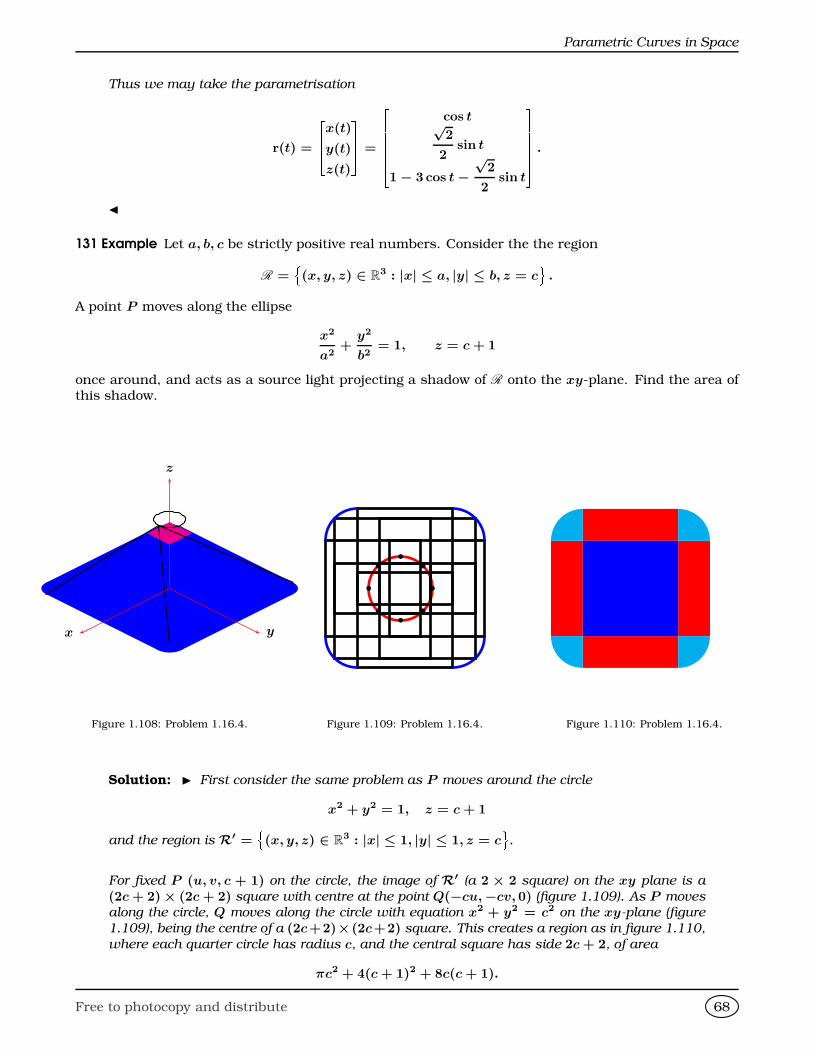
Parametric Curves in Space
Thus we may take the parametrisation
r(t) =
264x(t)
y(t)
z(t)
375 =
266664 cos t√2
2sin t
1− 3 cos t−√
2
2sin t
377775 .
J
131 Example Let a, b, c be strictly positive real numbers. Consider the the region
R =¦(x, y, z) ∈ R
3 : |x| ≤ a, |y| ≤ b, z = c©
.
A point P moves along the ellipse
x2
a2+
y2
b2= 1, z = c + 1
once around, and acts as a source light projecting a shadow of R onto the xy-plane. Find the area ofthis shadow.
x y
z
Figure 1.108: Problem 1.16.4.
b
b
b
b
b
b
b
b
Figure 1.109: Problem 1.16.4. Figure 1.110: Problem 1.16.4.
Solution: I First consider the same problem as P moves around the circle
x2 + y2 = 1, z = c + 1
and the region is R′ =¦(x, y, z) ∈ R
3 : |x| ≤ 1, |y| ≤ 1, z = c©
.
For fixed P (u, v, c + 1) on the circle, the image of R′ (a 2 × 2 square) on the xy plane is a
(2c + 2)× (2c + 2) square with centre at the point Q(−cu,−cv, 0) (figure 1.109). As P moves
along the circle, Q moves along the circle with equation x2 + y2 = c2 on the xy-plane (figure
1.109), being the centre of a (2c+2)×(2c+2) square. This creates a region as in figure 1.110,
where each quarter circle has radius c, and the central square has side 2c + 2, of area
πc2 + 4(c + 1)2 + 8c(c + 1).
Free to photocopy and distribute 68
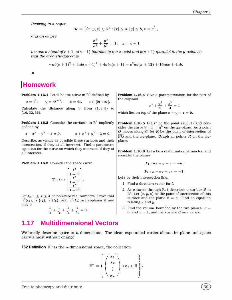
Chapter 1
Resizing to a region
R =¦(x, y, z) ∈ R
3 : |x| ≤ a, |y| ≤ b, z = c©
,
and an ellipsex2
a2+
y2
b2= 1, z = c + 1
we use instead of c + 1, a(c + 1) (parallel to the x-axis) and b(c + 1) (parallel to the y-axis), so
that the area shadowed is
πab(c + 1)2 + 4ab(c + 1)2 + 4abc(c + 1) = c2ab(π + 12) + 16abc + 4ab.
J
HomeworkProblem 1.16.1 Let C be the curve in R
3 defined by
x = t2, y = 4t3/2, z = 9t, t ∈ [0; +∞[.
Calculate the distance along C from (1, 4, 9) to(16, 32, 36).
Problem 1.16.2 Consider the surfaces in R3 implicitly
defined by
z − x2 − y2 − 1 = 0, z + x2 + y2 − 3 = 0.
Describe, as vividly as possible these surfaces and theirintersection, if they at all intersect. Find a parametric
equation for the curve on which they intersect, if they atall intersect.
Problem 1.16.3 Consider the space curve
−→r : t 7→
266664 t4
1 + t2
t3
1 + t2
t2
1 + t2
377775 .
Let tk, 1 ≤ k ≤ 4 be non-zero real numbers. Prove that−→r (t1),
−→r (t2),−→r (t3), and −→r (t4) are coplanar if and
only if1
t1+
1
t2+
1
t3+
1
t4= 0.
Problem 1.16.4 Give a parametrisation for the part ofthe ellipsoid
x2 +y2
9+
z2
4= 1
which lies on top of the plane x + y + z = 0.
Problem 1.16.5 Let P be the point (2, 0, 1) and con-
sider the curve C : z = y2 on the yz-plane. As a pointQ moves along C , let R be the point of intersection of←→PQ and the xy-plane. Graph all points R on the xy-plane.
Problem 1.16.6 Let a be a real number parameter, andconsider the planes
P1 : ax + y + z = −a,
P2 : x − ay + az = −1.
Let l be their intersection line.
1. Find a direction vector for l.
2. As a varies through R, l describes a surface S in
R3. Let (x, y, z) be the point of intersection of this
surface and the plane z = c. Find an equationrelating x and y.
3. Find the volume bounded by the two planes, x =0, and x = 1, and the surface S as c varies.
1.17 Multidimensional VectorsWe briefly describe space in n-dimensions. The ideas expounded earlier about the plane and spacecarry almost without change.
132 Definition Rn is the n-dimensional space, the collection
Rn =
8>>><>>>:x1
x2
...
xn
: xk ∈ R
9>>>=>>>; .
Free to photocopy and distribute 69
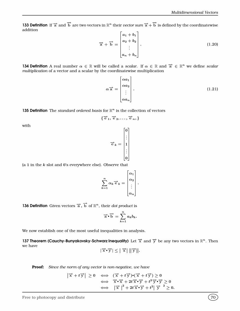
Multidimensional Vectors
133 Definition If−→a and−→b are two vectors in R
n their vector sum−→a +−→b is defined by the coordinatewise
addition
−→a +−→b =
2666664a1 + b1
a2 + b2
...
an + bn
3777775 . (1.20)
134 Definition A real number α ∈ R will be called a scalar. If α ∈ R and −→a ∈ Rn we define scalar
multiplication of a vector and a scalar by the coordinatewise multiplication
α−→a =
2666664αa1
αa2
...
αan
3777775 . (1.21)
135 Definition The standard ordered basis for Rn is the collection of vectors
−→e 1,−→e 2, . . . ,−→e n, with
−→e k =
26666666640...1...0
3777777775(a 1 in the k slot and 0’s everywhere else). Observe that
nXk=1
αk−→e k =
2666664α1
α2
...
αn
3777775 .
136 Definition Given vectors −→a ,−→b of R
n, their dot product is
−→a •−→b =
nXk=1
akbk.
We now establish one of the most useful inequalities in analysis.
137 Theorem (Cauchy-Bunyakovsky-Schwarz Inequality) Let −→x and −→y be any two vectors in Rn. Then
we have|−→x •−→y | ≤
−→x −→y .Proof: Since the norm of any vector is non-negative, we have−→x + t−→y
≥ 0 ⇐⇒ (−→x + t−→y )•(−→x + t−→y ) ≥ 0
⇐⇒ −→x •−→x + 2t−→x •−→y + t2−→y •−→y ≥ 0
⇐⇒−→x 2 + 2t−→x •−→y + t2
−→y 2 ≥ 0.
Free to photocopy and distribute 70
Chapter 1
This last expression is a quadratic polynomial in t which is always non-negative. As such its
discriminant must be non-positive, that is,
(2−→x •−→y )2 − 4(−→x 2)(−→y 2) ≤ 0 ⇐⇒ |−→x •−→y | ≤
−→x −→y ,giving the theorem.
The above proof works not just for Rn
but for any vector space (cf. below) that has an inner product.
The form of the Cauchy-Bunyakovsky-Schwarz most useful to us will be nXk=1
xkyk
≤ nXk=1
x2k
!1/2 nXk=1
y2k
!1/2
, (1.22)
for real numbers xk, yk.
138 Corollary (Triangle Inequality) Let −→a and−→b be any two vectors in R
n. Then we have−→a +−→b ≤ −→a + −→b .
Proof:||−→a +
−→b ||2 = (−→a +
−→b )•(−→a +
−→b )
= −→a •−→a + 2−→a •−→b +
−→b •−→b
≤ ||−→a ||2 + 2||−→a ||||−→b ||+ ||−→b ||2
= (||−→a ||+ ||−→b ||)2,
from where the desired result follows.
Again, the preceding proof is valid in any vector space that has a norm.
139 Definition Let −→x and −→y be two non-zero vectors in a vector space over the real numbers. Then the
angle (−→x ,−→y ) between them is given by the relation
cos (−→x ,−→y ) =−→x •−→y−→x −→y .
This expression agrees with the geometry in the case of the dot product for R2 and R
3.
140 Example Assume that ak, bk, ck, k = 1, . . . , n, are positive real numbers. Shew that nX
k=1
akbkck
!4
≤
nXk=1
a4k
! nX
k=1
b4k
! nX
k=1
c2k
!2
.
Solution: I Using CBS on
nXk=1
(akbk)ck once we obtain
nXk=1
akbkck ≤
nXk=1
a2kb2
k
!1/2 nXk=1
c2k
!1/2
.
Using CBS again on
nX
k=1
a2kb2
k
!1/2
we obtain
nXk=1
akbkck ≤
nXk=1
a2kb2
k
!1/2 nXk=1
c2k
!1/2
≤
nXk=1
a4k
!1/4 nXk=1
b4k
!1/4 nXk=1
c2k
!1/2
,
Free to photocopy and distribute 71
Multidimensional Vectors
which gives the required inequality. J
We now use the CBS inequality to establish another important inequality. We need some preparatorywork.
141 Lemma Let ak > 0, qk > 0, with
nXk=1
qk = 1. Then
limx→0
log
nX
k=1
qkaxk
!1/x
=nX
k=1
qk log ak.
Proof: Recall that log(1 + x) ∼ x as x→ 0. Thus
limx→0
log
nX
k=1
qkaxk
!1/x
= limx→0
logPn
k=1 qkaxk
x
= limx→0
Pnk=1 qk(ax
k − 1)
x
= limx→0
nXk=1
qk
(axk − 1)
x
=nX
k=1
qk log ak.
142 Theorem (Arithmetic Mean-Geometric Mean Inequality) Let ak ≥ 0. Then
n√
a1a2 · · ·an ≤a1 + a2 + ·+ an
n.
Proof: If bk ≥ 0, then by CBS
1
n
nXk=1
bk ≥
1
n
nXk=1
pbk
!2
. (1.23)
Successive applications of (1.23) yield the monotone decreasing sequence
1
n
nXk=1
ak ≥
1
n
nXk=1
√ak
!2
≥
1
n
nXk=1
4√
ak
!4
≥ . . . ,
which by Lemma 141 has limit
exp
1
n
nXk=1
log ak
!= n√
a1a2 · · ·an,
giving
n√
a1a2 · · ·an ≤a1 + a2 + ·+ an
n,
as wanted.
143 Example For any positive integer n > 1 we have
1 · 3 · 5 · · · · (2n− 1) < nn.
For, by AMGM,
1 · 3 · 5 · · · · (2n− 1) <
1 + 3 + 5 + · · ·+ (2n− 1)
n
n
=
n2
n
n
= nn.
Notice that since the factors are unequal we have strict inequality.
Free to photocopy and distribute 72
Chapter 1
144 Definition Let a1 > 0, a2 > 0, . . . , an > 0. Their harmonic mean is given by
n
1
a1
+1
a2
+ · · ·+ 1
an
.
As a corollary to AMGM we obtain
145 Corollary (Harmonic Mean-Geometric Mean Inequality) Let b1 > 0, b2 > 0, . . . , bn > 0. Then
n
1
b1
+1
b2
+ · · ·+ 1
bn
≤ (b1b2 · · · bn)1/n.
Proof: This follows by putting ak =1
bk
in Theorem 142 . For then1
b1
1
b2
· · · 1
bn
1/n
≤
1
b1
+1
b2
+ · · ·+ 1
bn
n.
Combining Theorem 142 and Corollary 145, we deduce
146 Corollary (Harmonic Mean-Arithmetic Mean Inequality) Let b1 > 0, b2 > 0, . . . , bn > 0. Then
n
1
b1
+1
b2
+ · · ·+ 1
bn
≤ b1 + b2 + · · ·+ bn
n.
147 Example Let ak > 0, and s = a1 + a2 + · · ·+ an. Prove that
nXk=1
s
s− ak
≥ n2
n− 1
andnX
k=1
ak
s− ak
≥ n
n− 1.
Solution: I Put bk =s
s− ak
. Then
nXk=1
1
bk
=nX
k=1
s− ak
s= n− 1
and from Corollary 146,
n
n− 1≤
Pnk=1
s
s− ak
n,
from where the first inequality is proved.
Free to photocopy and distribute 73
Multidimensional Vectors
Sinces
s− ak
− 1 =ak
s− ak
, we have
nXk=1
ak
s− ak
=nX
k=1
s
s− ak
− 1
=
nXk=1
s
s− ak
− n
≥ n2
n− 1− n
=n
n− 1.
J
HomeworkProblem 1.17.1 The Arithmetic Mean Geometric Mean
Inequality says that if ak ≥ 0 then
(a1a2 · · · an)1/n ≤ a1 + a2 + · · ·+ an
n.
Equality occurs if and only if a1 = a2 = . . . = an .In this exercise you will follow the steps of a proof by
George Polya.
1. Prove that ∀x ∈ R, x ≤ ex−1.
2. PutAk =
nak
a1 + a2 + · · ·+ an,
and Gn = a1a2 · · · an . Prove that
A1A2 · · ·An =nnGn
(a1 + a2 + · · ·+ an)n,
and that
A1 + A2 + · · ·+ An = n.
3. Deduce that
Gn ≤
a1 + a2 + · · ·+ an
n
n
.
4. Prove the AMGM inequality by assembling the re-sults above.
Problem 1.17.2 Demonstrate that if x1, x2, . . . , xn , are
strictly positive real numbers then
(x1 + x2 + . . . + xn)
1
x1+
1
x2+ . . . +
1
xn
≥ n2.
Problem 1.17.3 (USAMO 1978) Let a, b, c, d, e be real
numbers such that
a + b + c + d + e = 8, a2 + b2 + c2 + d2 + e2 = 16.
Maximise the value of e.
Problem 1.17.4 Find all positive real numbers
a1 ≤ a2 ≤ . . . ≤ an
such that
nXk=1
ak = 96,
nXk=1
a2k = 144,
nXk=1
a3k = 216.
Problem 1.17.5 Demonstrate that for integer n > 1 wehave,
n! <
n + 1
2
n
.
Problem 1.17.6 Let f(x) = (a + x)5(a − x)3, x ∈[−a;a]. Find the maximum value of de f using the AM-
GM inequality.
Problem 1.17.7 Prove that the sequence xn =1 +
1
n
n
,
n = 1, 2, . . . is strictly increasing.
Free to photocopy and distribute 74
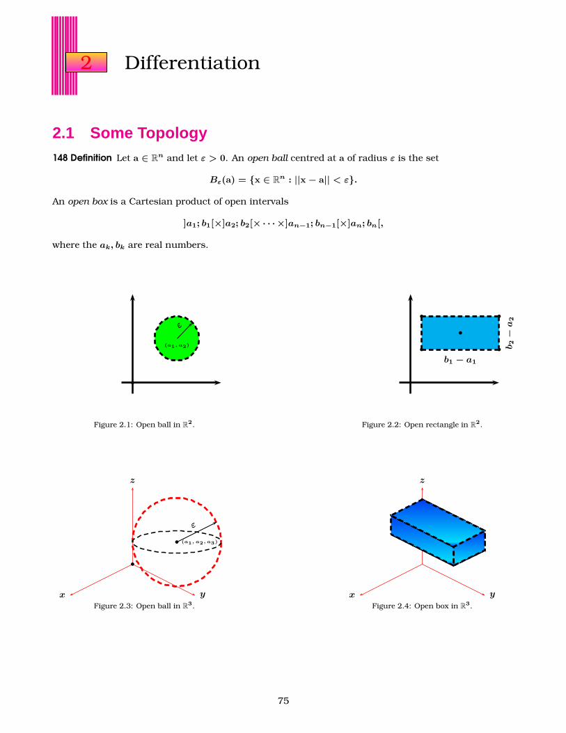
2 Differentiation
2.1 Some Topology148 Definition Let a ∈ R
n and let ε > 0. An open ball centred at a of radius ε is the set
Bε(a) = x ∈ Rn : ||x− a|| < ε.
An open box is a Cartesian product of open intervals
]a1; b1[×]a2; b2[×· · · ×]an−1; bn−1[×]an; bn[,
where the ak, bk are real numbers.
b
b
(a1, a2)
ε
Figure 2.1: Open ball in R2.
b b
bb
b1 − a1
b2−
a2
b
Figure 2.2: Open rectangle in R2.
x y
z
b
b
ε
(a1, a2, a3)
Figure 2.3: Open ball in R3.
x y
z
Figure 2.4: Open box in R3.
75
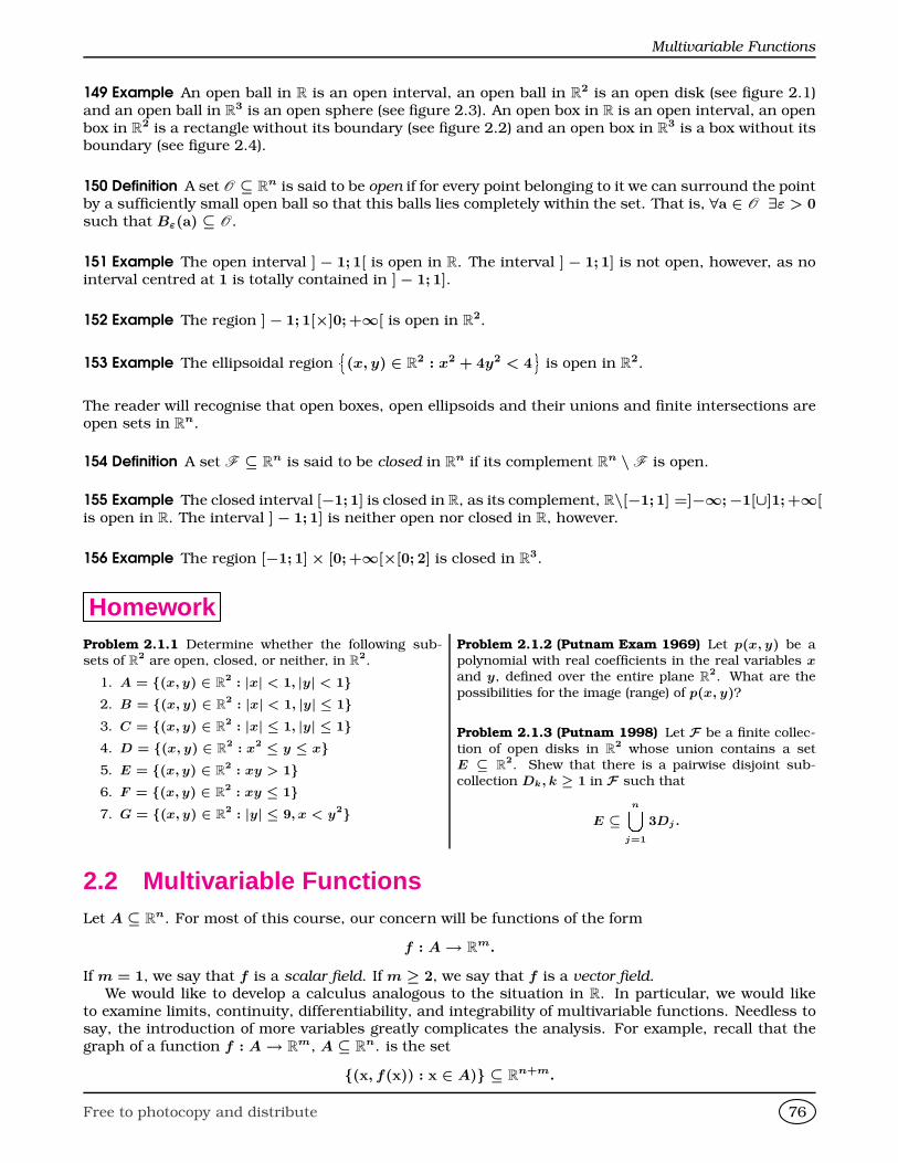
Multivariable Functions
149 Example An open ball in R is an open interval, an open ball in R2 is an open disk (see figure 2.1)
and an open ball in R3 is an open sphere (see figure 2.3). An open box in R is an open interval, an open
box in R2 is a rectangle without its boundary (see figure 2.2) and an open box in R
3 is a box without itsboundary (see figure 2.4).
150 Definition A set O ⊆ Rn is said to be open if for every point belonging to it we can surround the point
by a sufficiently small open ball so that this balls lies completely within the set. That is, ∀a ∈ O ∃ε > 0such that Bε(a) ⊆ O.
151 Example The open interval ] − 1; 1[ is open in R. The interval ] − 1; 1] is not open, however, as nointerval centred at 1 is totally contained in ]− 1; 1].
152 Example The region ]− 1; 1[×]0;+∞[ is open in R2.
153 Example The ellipsoidal region¦(x, y) ∈ R
2 : x2 + 4y2 < 4©
is open in R2.
The reader will recognise that open boxes, open ellipsoids and their unions and finite intersections areopen sets in R
n.
154 Definition A set F ⊆ Rn is said to be closed in R
n if its complement Rn \F is open.
155 Example The closed interval [−1; 1] is closed in R, as its complement, R\[−1; 1] =]−∞;−1[∪]1;+∞[is open in R. The interval ]− 1; 1] is neither open nor closed in R, however.
156 Example The region [−1; 1]× [0;+∞[×[0; 2] is closed in R3.
HomeworkProblem 2.1.1 Determine whether the following sub-sets of R
2 are open, closed, or neither, in R2.
1. A = (x, y) ∈ R2 : |x| < 1, |y| < 1
2. B = (x, y) ∈ R2 : |x| < 1, |y| ≤ 1
3. C = (x, y) ∈ R2 : |x| ≤ 1, |y| ≤ 1
4. D = (x, y) ∈ R2 : x2 ≤ y ≤ x
5. E = (x, y) ∈ R2 : xy > 1
6. F = (x, y) ∈ R2 : xy ≤ 1
7. G = (x, y) ∈ R2 : |y| ≤ 9, x < y2
Problem 2.1.2 (Putnam Exam 1969) Let p(x, y) be apolynomial with real coefficients in the real variables xand y, defined over the entire plane R
2. What are the
possibilities for the image (range) of p(x, y)?
Problem 2.1.3 (Putnam 1998) Let F be a finite collec-
tion of open disks in R2 whose union contains a set
E ⊆ R2. Shew that there is a pairwise disjoint sub-
collection Dk, k ≥ 1 in F such that
E ⊆n[
j=1
3Dj .
2.2 Multivariable FunctionsLet A ⊆ R
n. For most of this course, our concern will be functions of the form
f : A→ Rm.
If m = 1, we say that f is a scalar field. If m ≥ 2, we say that f is a vector field.We would like to develop a calculus analogous to the situation in R. In particular, we would like
to examine limits, continuity, differentiability, and integrability of multivariable functions. Needless tosay, the introduction of more variables greatly complicates the analysis. For example, recall that thegraph of a function f : A→ R
m, A ⊆ Rn. is the set
(x, f(x)) : x ∈ A) ⊆ Rn+m.
Free to photocopy and distribute 76
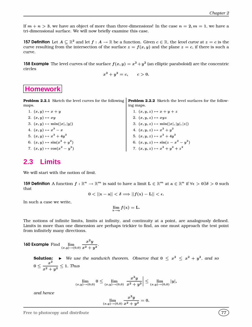
Chapter 2
If m + n > 3, we have an object of more than three-dimensions! In the case n = 2, m = 1, we have atri-dimensional surface. We will now briefly examine this case.
157 Definition Let A ⊆ R2 and let f : A → R be a function. Given c ∈ R, the level curve at z = c is the
curve resulting from the intersection of the surface z = f(x, y) and the plane z = c, if there is such acurve.
158 Example The level curves of the surface f(x, y) = x2 +y2 (an elliptic paraboloid) are the concentriccircles
x2 + y2 = c, c > 0.
Homework
Problem 2.2.1 Sketch the level curves for the following
maps.
1. (x, y) 7→ x + y
2. (x, y) 7→ xy
3. (x, y) 7→ min(|x|, |y|)4. (x, y) 7→ x3 − x
5. (x, y) 7→ x2 + 4y2
6. (x, y) 7→ sin(x2 + y2)
7. (x, y) 7→ cos(x2 − y2)
Problem 2.2.2 Sketch the level surfaces for the follow-
ing maps.
1. (x, y, z) 7→ x + y + z
2. (x, y, z) 7→ xyz
3. (x, y, z) 7→ min(|x|, |y|, |z|)4. (x, y, z) 7→ x2 + y2
5. (x, y, z) 7→ x2 + 4y2
6. (x, y, z) 7→ sin(z − x2 − y2)
7. (x, y, z) 7→ x2 + y2 + z2
2.3 LimitsWe will start with the notion of limit.
159 Definition A function f : Rn → R
m is said to have a limit L ∈ Rm at a ∈ R
n if ∀ε > 0∃δ > 0 suchthat
0 < ||x− a|| < δ =⇒ ||f(x)− L|| < ε.
In such a case we write,
limx→a
f(x) = L.
The notions of infinite limits, limits at infinity, and continuity at a point, are analogously defined.Limits in more than one dimension are perhaps trickier to find, as one must approach the test pointfrom infinitely many directions.
160 Example Find lim(x,y)→(0,0)
x2y
x2 + y2.
Solution: I We use the sandwich theorem. Observe that 0 ≤ x2 ≤ x2 + y2, and so
0 ≤ x2
x2 + y2≤ 1. Thus
lim(x,y)→(0,0)
0 ≤ lim(x,y)→(0,0)
x2y
x2 + y2
≤ lim(x,y)→(0,0)
|y|,
and hence
lim(x,y)→(0,0)
x2y
x2 + y2= 0.
Free to photocopy and distribute 77
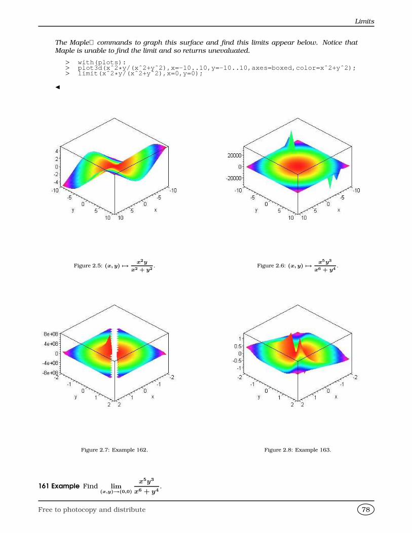
Limits
The Maple commands to graph this surface and find this limits appear below. Notice that
Maple is unable to find the limit and so returns unevaluated.
> with(plots):> plot3d(xˆ2 * y/(xˆ2+yˆ2),x=-10..10,y=-10..10,axes=boxed,color=xˆ 2+yˆ2);> limit(xˆ2 * y/(xˆ2+yˆ2),x=0,y=0);
J
Figure 2.5: (x, y) 7→ x2y
x2 + y2. Figure 2.6: (x, y) 7→ x5y3
x6 + y4.
Figure 2.7: Example 162. Figure 2.8: Example 163.
161 Example Find lim(x,y)→(0,0)
x5y3
x6 + y4.
Free to photocopy and distribute 78
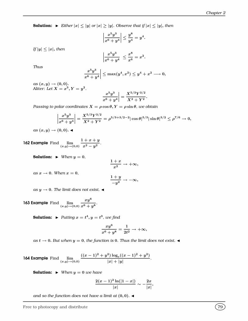
Chapter 2
Solution: I Either |x| ≤ |y| or |x| ≥ |y|. Observe that if |x| ≤ |y|, then x5y3
x6 + y4
≤ y8
y4= y4.
If |y| ≤ |x|, then x5y3
x6 + y4
≤ x8
x6= x2.
Thus x5y3
x6 + y4
≤ max(y4, x2) ≤ y4 + x2 −→ 0,
as (x, y)→ (0, 0).Aliter: Let X = x3, Y = y2. x5y3
x6 + y4
= X5/3Y 3/2
X2 + Y 2.
Passing to polar coordinates X = ρ cos θ, Y = ρ sin θ, we obtain x5y3
x6 + y4
= X5/3Y 3/2
X2 + Y 2= ρ5/3+3/2−2| cos θ|5/3| sin θ|3/2 ≤ ρ7/6 → 0,
as (x, y)→ (0, 0). J
162 Example Find lim(x,y)→(0,0)
1 + x + y
x2 − y2.
Solution: I When y = 0,1 + x
x2→ +∞,
as x→ 0. When x = 0,1 + y
−y2→ −∞,
as y → 0. The limit does not exist. J
163 Example Find lim(x,y)→(0,0)
xy6
x6 + y8.
Solution: I Putting x = t4, y = t3, we find
xy6
x6 + y8=
1
2t2→ +∞,
as t→ 0. But when y = 0, the function is 0. Thus the limit does not exist. J
164 Example Find lim(x,y)→(0,0)
((x− 1)2 + y2) loge((x− 1)2 + y2)
|x|+ |y| .
Solution: I When y = 0 we have
2(x− 1)2 ln(|1− x|)|x| ∼ −2x
|x| ,
and so the function does not have a limit at (0, 0). J
Free to photocopy and distribute 79
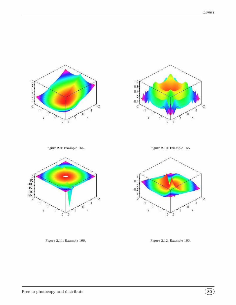
Limits
Figure 2.9: Example 164. Figure 2.10: Example 165.
Figure 2.11: Example 166. Figure 2.12: Example 163.
Free to photocopy and distribute 80
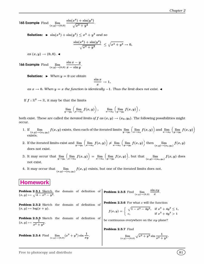
Chapter 2
165 Example Find lim(x,y)→(0,0)
sin(x4) + sin(y4)px4 + y4
.
Solution: I sin(x4) + sin(y4) ≤ x4 + y4 and sosin(x4) + sin(y4)px4 + y4
≤ Èx4 + y4 → 0,
as (x, y)→ (0, 0). J
166 Example Find lim(x,y)→(0,0)
sin x− y
x− sin y.
Solution: I When y = 0 we obtainsin x
x→ 1,
as x→ 0. When y = x the function is identically −1. Thus the limit does not exist. J
If f : R2 → R, it may be that the limits
limy→y0
lim
x→x0
f(x, y)
, lim
x→x0
lim
y→y0
f(x, y)
,
both exist. These are called the iterated limits of f as (x, y)→ (x0, y0). The following possibilities mightoccur.
1. If lim(x,y)→(x0,y0)
f(x, y) exists, then each of the iterated limits limy→y0
lim
x→x0
f(x, y)
and lim
x→x0
lim
y→y0
f(x, y)
exists.
2. If the iterated limits exist and limy→y0
lim
x→x0
f(x, y)
6= lim
x→x0
lim
y→y0
f(x, y)
then lim
(x,y)→(x0,y0)f(x, y)
does not exist.
3. It may occur that limy→y0
lim
x→x0
f(x, y)
= lim
x→x0
lim
y→y0
f(x, y)
, but that lim
(x,y)→(x0,y0)f(x, y) does
not exist.
4. It may occur that lim(x,y)→(x0,y0)
f(x, y) exists, but one of the iterated limits does not.
HomeworkProblem 2.3.1 Sketch the domain of definition of(x, y) 7→
p4− x2 − y2.
Problem 2.3.2 Sketch the domain of definition of(x, y) 7→ log(x + y).
Problem 2.3.3 Sketch the domain of definition of
(x, y) 7→ 1
x2 + y2.
Problem 2.3.4 Find lim(x,y)→(0,0)
(x2 + y2) sin1
xy.
Problem 2.3.5 Find lim(x,y)→(0,2)
sin xy
x.
Problem 2.3.6 For what c will the function
f(x, y) =
¨ p1− x2 − 4y2, if x2 + 4y2 ≤ 1,
c, if x2 + 4y2 > 1
be continuous everywhere on the xy-plane?
Problem 2.3.7 Find
lim(x,y)→(0,0)
px2 + y2 sin
1
x2 + y2.
Free to photocopy and distribute 81
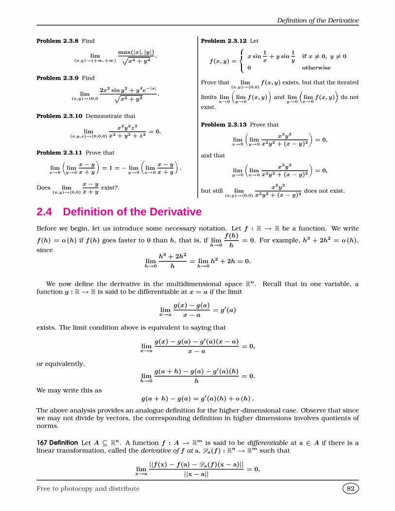
Definition of the Derivative
Problem 2.3.8 Find
lim(x,y)→(+∞,+∞)
max(|x|, |y|)px4 + y4
.
Problem 2.3.9 Find
lim(x,y)→(0,0
2x2 sin y2 + y4e−|x|px2 + y2
.
Problem 2.3.10 Demonstrate that
lim(x,y,z)→(0,0,0)
x2y2z2
x2 + y2 + z2= 0.
Problem 2.3.11 Prove that
limx→0
limy→0
x − y
x + y
= 1 = − lim
y→0
limx→0
x − y
x + y
.
Does lim(x,y)→(0,0)
x − y
x + yexist?.
Problem 2.3.12 Let
f(x, y) =
8<: x sin1
x+ y sin
1
yif x 6= 0, y 6= 0
0 otherwise
Prove that lim(x,y)→(0,0)
f(x, y) exists, but that the iterated
limits limx→0
limy→0
f(x, y)
and lim
y→0
limx→0
f(x, y)
do not
exist.
Problem 2.3.13 Prove that
limx→0
limy→0
x2y2
x2y2 + (x − y)2
= 0,
and that
limy→0
limx→0
x2y2
x2y2 + (x − y)2
= 0,
but still lim(x,y)→(0,0)
x2y2
x2y2 + (x − y)2does not exist.
2.4 Definition of the DerivativeBefore we begin, let us introduce some necessary notation. Let f : R → R be a function. We write
f(h) = o (h) if f(h) goes faster to 0 than h, that is, if limh→0
f(h)
h= 0. For example, h3 + 2h2 = o (h),
since
limh→0
h3 + 2h2
h= lim
h→0h2 + 2h = 0.
We now define the derivative in the multidimensional space Rn. Recall that in one variable, a
function g : R→ R is said to be differentiable at x = a if the limit
limx→a
g(x)− g(a)
x− a= g′(a)
exists. The limit condition above is equivalent to saying that
limx→a
g(x)− g(a)− g′(a)(x− a)
x− a= 0,
or equivalently,
limh→0
g(a + h)− g(a)− g′(a)(h)
h= 0.
We may write this as
g(a + h)− g(a) = g′(a)(h) + o (h) .
The above analysis provides an analogue definition for the higher-dimensional case. Observe that sincewe may not divide by vectors, the corresponding definition in higher dimensions involves quotients ofnorms.
167 Definition Let A ⊆ Rn. A function f : A → R
m is said to be differentiable at a ∈ A if there is alinear transformation, called the derivative of f at a, Da(f) : R
n → Rm such that
limx→a
||f(x)− f(a)− Da(f)(x− a)||||x− a|| = 0.
Free to photocopy and distribute 82
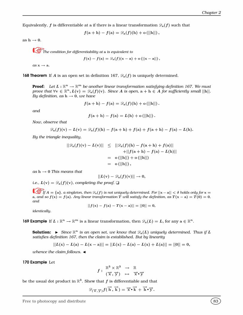
Chapter 2
Equivalently, f is differentiable at a if there is a linear transformation Da(f) such that
f(a + h)− f(a) = Da(f)(h) + o (||h||) ,
as h→ 0.
The condition for differentiability at a is equivalent to
f(x)− f(a) = Da(f)(x − a) + o (||x− a||) ,
as x→ a.
168 Theorem If A is an open set in definition 167, Da(f) is uniquely determined.
Proof: Let L : Rn → R
m be another linear transformation satisfying definition 167. We must
prove that ∀v ∈ Rn, L(v) = Da(f)(v). Since A is open, a + h ∈ A for sufficiently small ||h||.
By definition, as h→ 0, we have
f(a + h)− f(a) = Da(f)(h) + o (||h||) .
and
f(a + h)− f(a) = L(h) + o (||h||) .
Now, observe that
Da(f)(v)− L(v) = Da(f)(h)− f(a + h) + f(a) + f(a + h)− f(a)− L(h).
By the triangle inequality,
||Da(f)(v)− L(v)|| ≤ ||Da(f)(h)− f(a + h) + f(a)||+||f(a + h)− f(a)− L(h)||
= o (||h||) + o (||h||)= o (||h||) ,
as h→ 0 This means that
||L(v)− Da(f)(v)|| → 0,
i.e., L(v) = Da(f)(v), completing the proof.
If A = a, a singleton, then Da(f) is not uniquely determined. For ||x− a|| < δ holds only for x =a, and so f(x) = f(a). Any linear transformation T will satisfy the definition, as T (x − a) = T (0) = 0,
and
||f(x)− f(a)− T (x− a)|| = ||0|| = 0,
identically.
169 Example If L : Rn → R
m is a linear transformation, then Da(L) = L, for any a ∈ Rn.
Solution: I Since Rn is an open set, we know that Da(L) uniquely determined. Thus if L
satisfies definition 167, then the claim is established. But by linearity
||L(x)− L(a)− L(x− a)|| = ||L(x)− L(a)− L(x) + L(a)|| = ||0|| = 0,
whence the claim follows. J
170 Example Let
f :R
3 × R3 → R
(−→x ,−→y ) 7→ −→x •−→ybe the usual dot product in R
3. Shew that f is differentiable and that
D(−→x ,−→y )f(−→h ,−→k ) = −→x •
−→k +−→h •−→y .
Free to photocopy and distribute 83
The Jacobi Matrix
Solution: I We have
f(−→x +−→h ,−→y +
−→k )− f(−→x ,−→y ) = (−→x +
−→h )•(−→y +
−→k )−−→x •−→y
= −→x •−→y +−→x •−→k +−→h •−→y +
−→h •−→k −−→x •−→y
= −→x •−→k +−→h •−→y +
−→h •−→k .
As (−→h ,−→k ) → (
−→0 ,−→0 ), we have by the Cauchy-Buniakovskii-Schwarz inequality, |−→h •
−→k | ≤−→h −→k = o
−→h , which proves the assertion. J
Just like in the one variable case, differentiability at a point, implies continuity at that point.
171 Theorem Suppose A ⊆ Rn is open and f : A→ R
n is differentiable on A. Then f is continuous onA.
Proof: Given a ∈ A, we must shew that
limx→a
f(x) = f(a).
Since f is differentiable at a we have
f(x)− f(a) = Da(f)(x− a) + o (||x− a||) ,
and so
f(x)− f(a)→ 0,
as x→ a, proving the theorem.
HomeworkProblem 2.4.1 Let L : R
3 → R3 be a linear transforma-
tion and
F :R
3 → R3
−→x 7→ −→x × L(−→x ).
Shew that F is differentiable and that
Dx(F )(−→h ) = −→x × L(
−→h ) +
−→h × L(−→x ).
Problem 2.4.2 Let f : Rn → R, n ≥ 1, f(−→x ) =
−→x be the usual norm in R
n , with−→x 2 = −→x •−→x . Prove
that
Dx(f)(−→v ) =−→x •−→v−→x ,
for −→x 6= −→0 , but that f is not differentiable at−→0 .
2.5 The Jacobi MatrixWe now establish a way which simplifies the process of finding the derivative of a function at a givenpoint.
172 Definition Let A ⊆ Rn, f : A→ R
m, and put
f(x) =
2666664 f1(x1, x2, . . . , xn)
f2(x1, x2, . . . , xn)...
fm(x1, x2, . . . , xn)
3777775 .
Here fi : Rn → R. The partial derivative
∂fi
∂xj
(x) is defined as
∂fi
∂xj
(x) = limh→0
fi(x1, x2, . . . , xj + h, . . . , xn)− fi(x1, x2, . . . , xj, . . . , xn)
h,
whenever this limit exists.
Free to photocopy and distribute 84
Chapter 2
To find partial derivatives with respect to the j-th variable, we simply keep the other variables fixedand differentiate with respect to the j-th variable.
173 Example If f : R3 → R, and f(x, y, z) = x + y2 + z3 + 3xy2z3 then
∂f
∂x(x, y, z) = 1 + 3y2z3,
∂f
∂y(x, y, z) = 2y + 6xyz3,
and∂f
∂z(x, y, z) = 3z2 + 9xy2z2.
The Maple commands to find these follow.> f:=(x,y,z)->x+yˆ2+zˆ3+3 * x* yˆ2 * zˆ3;> diff(f(x,y,z),x);> diff(f(x,y,z),y);> diff(f(x,y,z),z);
Since the derivative of a function f : Rn → R
m is a linear transformation, it can be represented byaid of matrices. The following theorem will allow us to determine the matrix representation for Da(f)under the standard bases of R
n and Rm.
174 Theorem Let
f(x) =
2666664 f1(x1, x2, . . . , xn)
f2(x1, x2, . . . , xn)...
fm(x1, x2, . . . , xn)
3777775 .
Suppose A ⊆ Rn is an open set and f : A→ R
m is differentiable. Then each partial derivative∂fi
∂xj
(x)
exists, and the matrix representation of Dx(f) with respect to the standard bases of Rn and R
m is theJacobi matrix
f ′(x) =
26666666664∂f1
∂x1
(x)∂f1
∂x2
(x) · · · ∂f1
∂xn
(x)
∂f2
∂x1
(x)∂f2
∂x2
(x) · · · ∂f2
∂xn
(x)
......
......
∂fn
∂x1
(x)∂fn
∂x2
(x) · · · ∂fn
∂xn
(x)
37777777775 .
Proof: Let−→e j, 1 ≤ j ≤ n, be the standard basis for Rn. To obtain the Jacobi matrix, we must
compute Dx(f)(−→e j), which will give us the j-th column of the Jacobi matrix. Let f ′(x) = (Jij),and observe that
Dx(f)(−→e j) =
2666664J1j
J2j
...
Jnj
3777775 .
and put y = x + ε−→e j, ε ∈ R. Notice that
||f(y)− f(x)− Dx(f)(y − x)||||y− x||
=||f(x1, x2, . . . , xj + h, . . . , xn)− f(x1, x2, . . . , xj, . . . , xn)− εDx(f)(−→e j)||
|ε| .
Free to photocopy and distribute 85
The Jacobi Matrix
Since the sinistral side→ 0 as ε→ 0, the so does the i-th component of the numerator, and so,
|fi(x1, x2, . . . , xj + h, . . . , xn)− fi(x1, x2, . . . , xj, . . . , xn)− εJij||ε| → 0.
This entails that
Jij = limε→0
fi(x1, x2, . . . , xj + ε, . . . , xn)− fi(x1, x2, . . . , xj, . . . , xn)
ε=
∂fi
∂xj
(x) .
This finishes the proof.
Strictly speaking, the Jacobi matrix is not the derivative of a function at a point. It is a matrix
representation of the derivative in the standard basis of Rn
. We will abuse language, however, and refer
to f ′when we mean the Jacobi matrix of f .
175 Example Let f : R3 → R
2 be given by
f(x, y) = (xy + yz, loge xy).
Compute the Jacobi matrix of f .
Solution: I The Jacobi matrix is the 2× 3 matrix
f ′(x, y) =
2664∂f1
∂x(x, y)
∂f1
∂y(x, y)
∂f1
∂z(x, y)
∂f2
∂x(x, y)
∂f2
∂y(x, y)
∂f2
∂z(x, y)
3775 =
24y x + z y1
x
1
y0
35 .
J
176 Example Let f(ρ, θ, z) = (ρ cos θ, ρ sin θ, z) be the function which changes from cylindrical coordi-nates to Cartesian coordinates. We have
f ′(ρ, θ, z) =
264cos θ −ρ sin θ 0
sin θ ρ cos θ 0
0 0 1
375 .
177 Example Let f(ρ, φ, θ) = (ρ cos θ sin φ, ρ sin θ sin φ, ρ cos φ) be the function which changes fromspherical coordinates to Cartesian coordinates. We have
f ′(ρ, φ, θ) =
264cos θ sin φ ρ cos θ cos φ −ρ sin φ sin θ
sin θ sin φ ρ sin θ cos φ ρ cos θ sin φ
cos φ −ρ sin φ 0
375 .
The Jacobi matrix provides a convenient computational tool to compute the derivative of a functionat a point. Thus differentiability at a point implies that the partial derivatives of the function exist atthe point. The converse, however, is not true.
178 Example Let f : R2 → R be given by
f(x, y) =
8><>: y if x = 0,
x if y = 0,
1 if xy 6= 0.
Free to photocopy and distribute 86
Chapter 2
Observe that f is not continuous at (0, 0) (f(0, 0) = 0 but f(x, y) = 1 for values arbitrarily close to
(0, 0)), and hence, it is not differentiable there. We have however,∂f
∂x(0, 0) =
∂f
∂y(0, 0) = 1. Thus even
if both partial derivatives exist at (0, 0) is no guarantee that the function will be differentiable at (0, 0).You should also notice that both partial derivatives are not continuous at (0, 0).
We have, however, the following.
179 Theorem Let A ⊆ Rn be an open set, and let f : R
n → Rm. Put f =
266664 f1
f2
. . .
fm
377775. If each of the partial
derivatives Djfi exists and is continuous on A, then f is differentiable on A.
The concept of repeated partial derivatives is akin to the concept of repeated differentiation. Similarlywith the concept of implicit partial differentiation. The following examples should be self-explanatory.
180 Example Let f(u, v, w) = euv cos w. Determine∂2
∂u∂vf(u, v, w) at (1,−1,
π
4).
Solution: I We have
∂2
∂u∂v(euv cos w) =
∂
∂u(eu cos w) = eu cos w,
which ise√
2
2at the desired point. J
181 Example The equation zxy + (xy)z + xy2z3 = 3 defines z as an implicit function of x and y. Find∂z
∂xand
∂z
∂yat (1, 1, 1).
Solution: I We have∂
∂xzxy =
∂
∂xexy log z
=
y log z +
xy
z
∂z
∂x
zxy,
∂
∂x(xy)z =
∂
∂xez log xy
=
∂z
∂xlog xy +
z
x
(xy)z,
∂
∂xxy2z3 = y2z3 + 3xy2z2 ∂z
∂x,
Hence, at (1, 1, 1) we have
∂z
∂x+ 1 + 1 + 3
∂z
∂x= 0 =⇒ ∂z
∂x= −1
2.
Similarly,∂
∂yzxy =
∂
∂yexy log z
=
x log z +
xy
z
∂z
∂y
zxy,
Free to photocopy and distribute 87
The Jacobi Matrix
∂
∂y(xy)z =
∂
∂yez log xy
=
∂z
∂ylog xy +
z
y
(xy)z,
∂
∂yxy2z3 = 2xyz3 + 3xy2z2 ∂z
∂y,
Hence, at (1, 1, 1) we have
∂z
∂y+ 1 + 2 + 3
∂z
∂y= 0 =⇒ ∂z
∂y= −3
4.
J
Just like in the one-variable case, we have the following rules of differentiation. Let A ⊆ Rn, B ⊆ R
m
be open sets f, g : A → Rm, α ∈ R, be differentiable on A, h : B → R
l be differentiable on B, andf(A) ⊆ B. Then we have
• Addition Rule: Dx((f + αg)) = Dx(f) + αDx(g).
• Chain Rule: Dx((h f)) =Df (x)(h)
(Dx(f)).
Since composition of linear mappings expressed as matrices is matrix multiplication, the Chain Ruletakes the alternative form when applied to the Jacobi matrix.
(h f)′ = (h′ f)(f ′). (2.1)
182 Example Let
f(u, v) =
264 uev
u + v
uv
375 ,
h(x, y) =
"x2 + y
y + z
#.
Find (f h)′(x, y).
Solution: I We have
f ′(u, v) =
264ev uev
1 1
v u
375 ,
and
h′(x, y) =
"2x 1 0
0 1 1
#.
Observe also that
f ′(h(x, y)) =
264 ey+z (x2 + y)ey+z
1 1
y + z x2 + y
375 .
Free to photocopy and distribute 88
Chapter 2
Hence
(f h)′(x, y) = f ′(h(x, y))h′(x, y)
=
266664 ey+z (x2 + y)ey+z
1 1
y + z x2 + y
3777752642x 1 0
0 1 1
375=
266664 2xey+z (1 + x2 + y)ey+z (x2 + y)ey+z
2x 2 1
2xy + 2xz x2 + 2y + z x2 + y
377775 .
J
183 Example Let
f : R2 → R, f(u, v) = u2 + ev,
u, v : R3 → R u(x, y) = xz, v(x, y) = y + z.
Put h(x, y) = f
"u(x, y, z)
v(x, y, z)
#. Find the partial derivatives of h.
Solution: I Put g : R3 → R
2, g(x, y) =
"u(x, y)
v(x, y
#=
"xz
y + z
#. Observe that h = f g. Now,
g′(x, y) =
"z 0 x
0 1 1
#,
f ′(u, v) =2u ev
,
f ′(h(x, y)) =2xz ey+z
.
Thus ∂h
∂x(x, y)
∂h
∂y(x, y)
∂h
∂z(x, y)
= h′(x, y)
= (f ′(g(x, y)))(g′(x, y))
=
2xz ey+z
264z 0 x
0 1 1
375=
2xz2 ey+z 2x2z + ey+z
.
Equating components, we obtain∂h
∂x(x, y) = 2xz2,
∂h
∂y(x, y) = ey+z,
∂h
∂z(x, y) = 2x2z + ey+z.
J
Under certain conditions we may differentiate under the integral sign.
Free to photocopy and distribute 89
The Jacobi Matrix
184 Theorem (Differentiation under the integral sign) Let f : [a, b] × Y → R be a function, with [a, b]being a closed interval, and Y being a closed and bounded subset of R. Suppose that both f(x, y) and∂
∂xf(x, y) are continuous in the variables x and y jointly. Then
ZY
f(x.y) dy exists as a continuously
differentiable function of x on [a, b], with derivative
d
dx
ZY
f(x, y) dy =
ZY
∂
∂xf(x, y) dy.
185 Example Prove that
F (x) =
Z π/2
0log(sin2 θ + x2 cos2 θ)dθ = π log
x + 1
2.
Solution: I Differentiating under the integral,
F ′(x) =
Z π/2
0
∂
∂xlog(sin2 θ + x2 cos2 θ)dθ
= 2x
Z π/2
0
cos2 θ
sin2 θ + x2 cos2 θdθ
. The above implies that
(x2 − 1)
2x· F ′(x) =
Z π/2
0
(x2 − 1) cos2 θ
sin2 θ + x2 cos2 θdθ
=
Z π/2
0
x2 cos2 θ + sin2 θ − 1
sin2 θ + x2 cos2 θdθ
=π
2−Z π/2
0
dθ
sin2 θ + x2 cos2 θ
=π
2−Z π/2
0
sec2 θdθ
tan2 θ + x2
=π
2− 1
xarctan
tan θ
x
π/2
0
=π
2− π
2x,
which in turn implies that for x > 0, x 6= 1,
F ′(x) =2x
x2 − 1
π
2− π
2x
=
π
x + 1.
For x = 1 one sees immediately that F ′(1) = 2
Z π/2
0
cos2 θdθ =π
2, agreeing with the formula.
Now,
F ′(x) =π
x + 1=⇒ F (x) = π log(x + 1) + C.
Since F (1) =
Z π/2
0log 1dθ = 0, we gather that C = −π log 2. Finally thus
F (x) = π log(x + 1)− π log 2 = π logx + 1
2.
J
Under certain conditions, the interval of integration in the above theorem need not be compact.
186 Example Given that
Z +∞
0
sin x
xdx =
π
2, compute
Z +∞
0
sin2 x
x2dx.
Free to photocopy and distribute 90
Chapter 2
Solution: I Put I(a) =
Z +∞
0
sin2 ax
x2dx, with a ≥ 0. Differentiating both sides with respect
to a, and making the substitution u = 2ax,
I′(a) =
Z +∞
0
2x sin ax cos ax
x2dx
=
Z +∞
0
sin 2ax
xdx
=
Z +∞
0
sin u
udu
=π
2.
Integrating each side gives
I(a) =π
2a + C.
Since I(0) = 0, we gather that C = 0. The desired integral is I(1) =π
2. J
HomeworkProblem 2.5.1 Let f : [0;+∞[×]0;+∞[→ R, f(r, t) =
tne−r2/4t, where n is a constant. Determine n suchthat
∂f
∂t=
1
r2
∂
∂r
r2 ∂f
∂r
.
Problem 2.5.2 Let
f : R2 → R, f(x, y) = min(x, y2).
Find∂f(x, y)
∂xand
∂f(x, y)
∂y.
Problem 2.5.3 Let f : R2 → R
2 and g : R3 → R
2 begiven by
f(x, y) =
xy2
x2y
, g(x, y, z) =
x − y + 2z
xy
.
Compute (f g)′(1, 0, 1), if at all defined. If undefined,explain. Compute (g f)′(1, 0), if at all defined. If un-defined, explain.
Problem 2.5.4 Let f(x, y) =
xy
x + y
and g(x, y) =264x − y
x2y2
x + y
375 Find (g f)′(0, 1).
Problem 2.5.5 Suppose g : R → R is continuous anda ∈ R is a constant. Find the partial derivatives withrespect to x and y of
f : R2 → R, f(x, y) =
Z x2y
a
g(t) dt.
Problem 2.5.6 Given that
Z b
0
dx
x2 + a2=
1
aarctan
b
a,
evaluate
Z b
0
dx
(x2 + a2)2.
Problem 2.5.7 Prove thatZ +∞
0
arctan ax − arctan x
xdx =
π
2log π.
Problem 2.5.8 Assuming that the equation xy2 +3z =cos z2 defines z implicitly as a function of x and y, find∂z
∂x.
Problem 2.5.9 If w = euv and u = r + s, v = rs,
determine∂w
∂r.
Problem 2.5.10 Let z be an implicitly-defined function
of x and y through the equation (x+z)2 +(y +z)2 = 8.
Find∂z
∂xat (1, 1, 1).
2.6 Gradients and Directional DerivativesA function
f :R
n → Rm
x 7→ f(x)
Free to photocopy and distribute 91
Gradients and Directional Derivatives
is called a vector field. If m = 1, it is called a scalar field.
187 Definition Let
f :R
n → R
x 7→ f(x)
be a scalar field. The gradient of f is the vector defined and denoted by
∇f(x) =
26666666664∂f
∂x1
(x)
∂f
∂x2
(x)
...∂f
∂xn
(x)
37777777775 .
The gradient operator is the operator
∇ =
26666666664∂
∂x1∂
∂x2...∂
∂xn
37777777775 .
188 Theorem Let A ⊆ Rn be open and let f : A→ R be a scalar field, and assume that f is differentiable
in A. Let K ∈ R be a constant. Then∇f(x) is orthogonal to the surface implicitly defined by f(x) = K.
Proof: Let
c :R → R
n
t 7→ c(t)
be a curve lying on this surface. Choose t0 so that c(t0) = x. Then
(f c)(t0) = f(c(t)) = K,
and using the chain rule
f ′(c(t0))c′(t0) = 0,
which translates to
(∇f(x))•(c′(t0)) = 0.
Since c′(t0) is tangent to the surface and its dot product with ∇f(x) is 0, we conclude that
∇f(x) is normal to the surface.
Let θ be the angle between ∇f(x) and c′(t0). Since
|(∇f(x))•(c′(t0))| = ||∇f(x)||||c′(t0)|| cos θ,
∇f(x) is the direction in which f is changing the fastest.
189 Example Find a unit vector normal to the surface x3 + y3 + z = 4 at the point (1, 1, 2).
Solution: I Here f(x, y, z) = x3 + y3 + z − 4 has gradient
∇f(x, y, z) =
2643x2
3y2
1
375Free to photocopy and distribute 92
Chapter 2
which at (1, 1, 2) is
264331
375. Normalising this vector we obtain2666664 3√193√191√19
3777775 .
J
190 Example Find the direction of the greatest rate of increase of f(x, y, z) = xyez at the point (2, 1, 2).
Solution: I The direction is that of the gradient vector. Here
∇f(x, y, z) =
264 yez
xez
xyez
375which at (2, 1, 2) becomes
264 e2
2e2
2e2
375 . Normalising this vector we obtain
1√5
264122
375 .
J
191 Example Let f : R3 → R be given by
f(x, y, z) = x + y2 − z2.
Find the equation of the tangent plane to f at (1, 2, 3).
Solution: I A vector normal to the plane is ∇f(1, 2, 3). Now
∇f(x, y, z) =
264 1
2y
−2z
375which is 264 1
4
−6
375at (1, 2, 3). The equation of the tangent plane is thus
1(x− 1) + 4(y − 2)− 6(z − 3) = 0,
or
x + 4y − 6z = −9.
J
Free to photocopy and distribute 93

Gradients and Directional Derivatives
192 Definition Let
f :R
n → Rn
x 7→ f(x)
be a vector field with
f(x) =
2666664f1(x)
f2(x)...
fn(x)
3777775 .
The divergence of f is defined and denoted by
divf(x) = ∇•f(x) =∂f1
∂x1
(x) +∂f2
∂x2
(x) + · · ·+ ∂fn
∂xn
(x) .
193 Example If f(x, y, z) = (x2, y2, yez2
) then
divf(x) = 2x + 2y + 2yzez2
.
194 Definition Let gk : Rn → R
n, 1 ≤ k ≤ n − 2 be vector fields with gi = (gi1, gi2, . . . , gin). Then thecurl of (g1, g2, . . . , gn−2)
curl(g1, g2, . . . , gn−2)(x) = det
2666666666664e1 e2 · · · en
∂
∂x1
∂
∂x2
· · · ∂
∂xn
g11(x) g12(x) · · · g1n(x)
g21(x) g22(x) . . . g2n(x)...
......
...
g(n−2)1(x) g(n−2)2(x) . . . g(n−2)n(x)
3777777777775 .
195 Example If f(x, y, z) = (x2, y2, yez2
) then
curlf((x, y, z)) = ∇× f(x, y, z) = (ez2
)i.
196 Example If f(x, y, z, w) = (exyz, 0, 0, w2), g(x, y, z, w) = (0, 0, z, 0) then
curl(f, g)(x, y, z, w) = det
2666664 e1 e2 e3 e4
∂
∂x1
∂
∂x2
∂
∂x3
∂
∂x4
exyz 0 0 w2
0 0 z 0
3777775 = (xz2exyz)e4.
197 Definition Let A ⊆ Rn be open and let f : A → R be a scalar field, and assume that f is differen-
tiable in A. Let −→v ∈ Rn \ 0 be such that x+ t−→v ∈ A for sufficiently small t ∈ R. Then the directional
derivative of f in the direction of −→v at the point x is defined and denoted by
D−→v f(x) = limt→0
f(x + t−→v )− f(x)
t.
Some authors require that the vector −→v in definition 197 be a unit vector.
Free to photocopy and distribute 94
Chapter 2
198 Theorem Let A ⊆ Rn be open and let f : A→ R be a scalar field, and assume that f is differentiable
in A. Let −→v ∈ Rn \ −→0 be such that −→x + t−→v ∈ A for sufficiently small t ∈ R. Then the directional
derivative of f in the direction of −→v at the point −→x is given by
∇f(x)•−→v .
199 Example Find the directional derivative of f(x, y, z) = x3 + y3 − z2 in the direction of
264123
375.
Solution: I We have
∇f(x, y, z) =
2643x2
3y2
−2z
375and so
∇f(x, y, z)•−→v = 3x2 + 6y2 − 6z.
J
HomeworkProblem 2.6.1 Let f(x, y, z) = xeyz . Find
(∇f)(2, 1, 1).
Problem 2.6.2 Let f(x, y, z) =
264xz
exy
z
375. Find
(∇ × f)(2, 1, 1).
Problem 2.6.3 Find the tangent plane to the surfacex2
2− y2 − z2 = 0 at the point (2,−1, 1).
Problem 2.6.4 Find the point on the surface
x2 + y2 − 5xy + xz − yz = −3
for which the tangent plane is x − 7y = −6.
Problem 2.6.5 Find a vector pointing in the directionin which f(x, y, z) = 3xy − 9xz2 + y increases most
rapidly at the point (1, 1, 0).
Problem 2.6.6 Let D−→u f(x, y) denote the directionalderivative of f at (x, y) in the direction of the unit vector−→u . If ∇f(1, 2) = 2
−→i − −→j , find D( 3
5, 45)f(1, 2).
Problem 2.6.7 Use a linear approximation of the func-
tion f(x, y) = ex cos 2y at (0, 0) to estimate f(0.1, 0.2).
Problem 2.6.8 Prove that
∇ • (u× v) = v • (∇ × u)− u • (∇ × v).
Problem 2.6.9 Find the point on the surface
2x2 + xy + y2 + 4x + 8y − z + 14 = 0
for which the tangent plane is 4x + y − z = 0.
Problem 2.6.10 Let φ : R3 → R be a scalar field, and
let U, V : R3 → R
3 be vector fields. Prove that
1. ∇•φV = φ∇•V + V•∇φ
2. ∇ × φV = φ∇ × V + (∇φ)× V
3. ∇ × (∇φ) =−→0
4. ∇•(∇ × V) = 0
5. ∇(U•V) = (U•∇)V + (V•∇)U + U× (∇×V) ++V × (∇ × U)
Problem 2.6.11 Find the angles made by the gradient
of f(x, y) = x√
3 + y at the point (1, 1) with the coordi-
nate axes.
2.7 Levi-Civitta and Einstein
In this section, unless otherwise noted, we are dealing in the space R3
and so, subscripts are in the
set 1, 2, 3.
Free to photocopy and distribute 95
Levi-Civitta and Einstein
200 Definition (Einstein’s Summation Convention) In any expression containing subscripted variables ap-pearing twice (and only twice) in any term, the subscripted variables are assumed to be summed over.
In order to emphasise that we are using Einstein’s convention, we will enclose any terms under
consideration with < · =.
201 Example Using Einstein’s Summation convention, the dot product of two vectors −→x ∈ Rn and−→y ∈ R
n can be written as
−→x •−→y =nX
i=1
xiyi = <xtyt = .
202 Example Given that ai, bj, ck, dl are the components of vectors in R3, −→a ,
−→b ,−→c ,
−→d respectively,
what is the meaning of<aibickdk=?
Solution: I We have
<aibickdk= =3X
i=1
aibi < ckdk= = −→a •−→b < ckdk= = −→a •
−→b
3Xk=1
ckdk = (−→a •−→b )(−→c •
−→d ).
J
203 Example Using Einstein’s Summation convention, the ij-th entry (AB)ij of the product of twomatrices A ∈ Mm×n(R) and B ∈Mn×r(R) can be written as
(AB)ij =nX
k=1
AikBkj = <AitBtj = .
204 Example Using Einstein’s Summation convention, the trace tr (A) of a square matrix A ∈Mn×n(R)
is tr (A) =nX
t=1
Att = <Att=.
205 Example Demonstrate, via Einstein’s Summation convention, that if A, B are two n× n matrices,then
tr (AB) = tr (BA) .
Solution: I We have
tr (AB) = tr ((AB)ij) = tr (<AikBkj=) = < < AtkBkt = =,
and
tr (BA) = tr ((BA)ij) = tr (<BikAkj=) = < < BtkAkt = =,
from where the assertion follows, since the indices are dummy variables and can be ex-
changed. J
206 Definition (Kroenecker’s Delta) The symbol δij is defined as follows:
δij =
(0 if i 6= j
1 if i = j.
207 Example It is easy to see that <δikδkj= =3X
k=1
δikδkj = δij .
Free to photocopy and distribute 96
Chapter 2
208 Example We see that
<δijaibj= =3X
i=1
3Xj=1
δijaibj =Xk=1
akbk = −→a •−→b .
Recall that a permutation of distinct objects is a reordering of them. The 3! = 6 permutations of theindex set 1, 2, 3 can be classified into even or odd. We start with the identity permutation 123 andsay it is even. Now, for any other permutation, we will say that it is even if it takes an even number oftranspositions (switching only two elements in one move) to regain the identity permutation, and oddif it takes an odd number of transpositions to regain the identity permutation. Since
231→ 132→ 123, 312→ 132→ 123,
the permutations 123 (identity), 231, and 312 are even. Since
132→ 123, 321→ 123, 213→ 123,
the permutations 132, 321, and 213 are odd.
209 Definition (Levi-Civitta’s Alternating Tensor) The symbol εjkl is defined as follows:
εjkl =
8>>>>><>>>>>: 0 if j, k, l 6= 1, 2, 3
−1 if
1 2 3
j k l
!is an odd permutation
+1 if
1 2 3
j k l
!is an even permutation
In particular, if one subindex is repeated we have εrrs = εrsr = εsrr = 0. Also,
ε123 = ε231 = ε312 = 1, ε132 = ε321 = ε213 = −1.
210 Example Using the Levi-Civitta alternating tensor and Einstein’s summation convention, the cross
product can also be expressed, if−→i = −→e1 ,
−→j = −→e2 ,
−→k = −→e3 , then
−→x ×−→y = <εjkl(akbl)−→ej = .
211 Example If A = [aij] is a 3× 3 matrix, then, using the Levi-Civitta alternating tensor,
det A = <εijka1ia2ja3k = .
212 Example Let −→x ,−→y ,−→z be vectors in R3. Then
−→x • (−→y ×−→z ) = <xi(−→y ×−→z )i= = <xiεikl(ykzl) = .
Homework
Problem 2.7.1 Let −→x ,−→y ,−→z be vectors in R3. Demon- strate that
<xiyizj= = (−→x •−→y )−→z .
Free to photocopy and distribute 97
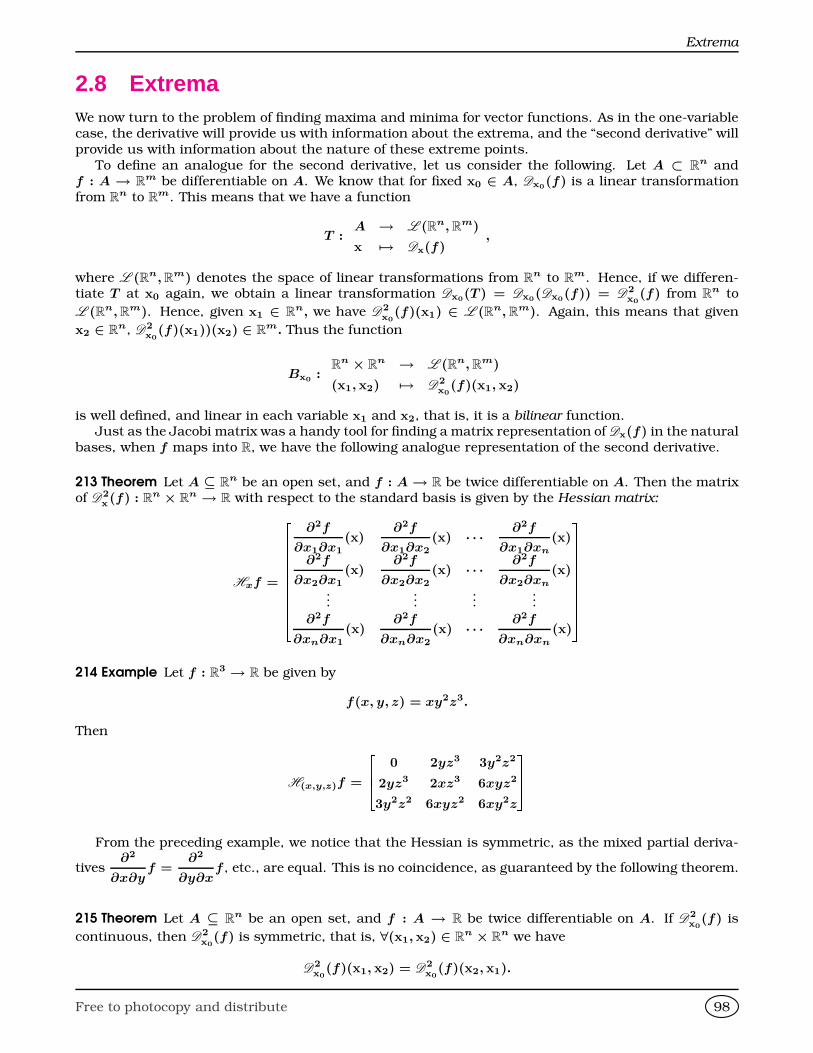
Extrema
2.8 ExtremaWe now turn to the problem of finding maxima and minima for vector functions. As in the one-variablecase, the derivative will provide us with information about the extrema, and the “second derivative” willprovide us with information about the nature of these extreme points.
To define an analogue for the second derivative, let us consider the following. Let A ⊂ Rn and
f : A → Rm be differentiable on A. We know that for fixed x0 ∈ A, Dx0(f) is a linear transformation
from Rn to R
m. This means that we have a function
T :A → L (Rn, R
m)
x 7→ Dx(f),
where L (Rn, Rm) denotes the space of linear transformations from R
n to Rm. Hence, if we differen-
tiate T at x0 again, we obtain a linear transformation Dx0(T ) = Dx0(Dx0(f)) = D2x0
(f) from Rn to
L (Rn, Rm). Hence, given x1 ∈ R
n, we have D2x0
(f)(x1) ∈ L (Rn, Rm). Again, this means that given
x2 ∈ Rn, D
2x0
(f)(x1))(x2) ∈ Rm. Thus the function
Bx0 :R
n × Rn → L (Rn, R
m)
(x1, x2) 7→ D2x0
(f)(x1, x2)
is well defined, and linear in each variable x1 and x2, that is, it is a bilinear function.Just as the Jacobi matrix was a handy tool for finding a matrix representation of Dx(f) in the natural
bases, when f maps into R, we have the following analogue representation of the second derivative.
213 Theorem Let A ⊆ Rn be an open set, and f : A→ R be twice differentiable on A. Then the matrix
of D2x(f) : R
n × Rn → R with respect to the standard basis is given by the Hessian matrix:
Hxf =
26666666664∂2f
∂x1∂x1
(x)∂2f
∂x1∂x2
(x) · · · ∂2f
∂x1∂xn
(x)
∂2f
∂x2∂x1
(x)∂2f
∂x2∂x2
(x) · · · ∂2f
∂x2∂xn
(x)
......
......
∂2f
∂xn∂x1
(x)∂2f
∂xn∂x2
(x) · · · ∂2f
∂xn∂xn
(x)
37777777775214 Example Let f : R
3 → R be given by
f(x, y, z) = xy2z3.
Then
H(x,y,z)f =
264 0 2yz3 3y2z2
2yz3 2xz3 6xyz2
3y2z2 6xyz2 6xy2z
375From the preceding example, we notice that the Hessian is symmetric, as the mixed partial deriva-
tives∂2
∂x∂yf =
∂2
∂y∂xf , etc., are equal. This is no coincidence, as guaranteed by the following theorem.
215 Theorem Let A ⊆ Rn be an open set, and f : A → R be twice differentiable on A. If D
2x0
(f) is
continuous, then D2x0
(f) is symmetric, that is, ∀(x1, x2) ∈ Rn × R
n we have
D2x0
(f)(x1, x2) = D2x0
(f)(x2, x1).
Free to photocopy and distribute 98
Chapter 2
We are now ready to study extrema in several variables. The basic theorems resemble those ofone-variable calculus. First, we make some analogous definitions.
216 Definition Let A ⊆ Rn be an open set, and f : A → R. If there is some open ball Bx0(r) on which
∀x ∈ Bx0(r), f(x0) ≥ f(x), we say that f(x0) is a local maximum of f . Similarly, if there is some openball Bx1(r) on which ∀x ∈ Bx0(r
′), f(x1) ≤ f(x), we say that f(x1) is a local maximum of f . A pointis called an extreme point if it is either a local minimum or local maximum. A point t is called a critical
point if f is differentiable at t and Dt(f) = 0. A critical point which is neither a maxima nor a minimais called a saddle point.
217 Theorem Let A ⊆ Rn be an open set, and f : A → R be differentiable on A. If x0 is an extreme
point, then Dx0(f) = 0, that is, x0 is a critical point. Moreover, if f is twice-differentiable with contin-uous second derivative and x0 is a critical point such that Hx0f is negative definite, then f has a localmaximum at x0. If Hx0f is positive definite, then f has a local minimum at x0. If Hx0f is indefinite,then f has a saddle point. If Hx0f is semi-definite (positive or negative), the test is inconclusive.
218 Example Find the critical points of
f :R
2 → R
(x, y) 7→ x2 + xy + y2 + 2x + 3y
and investigate their nature.
Solution: I We have
(∇f)(x, y) =
"2x + y + 2
x + 2y + 3
#,
and so to find the critical points we solve
2x + y + 2 = 0,
x + 2y + 3 = 0,
which yields x = −1
3, y = −4
3. Now,
H(x,y)f =
"2 1
1 2
#,
which is positive definite, since ∆1 = 2 > 0 and ∆2 = det
"2 1
1 2
#= 3 > 0. Thus x0 =
−1
3,−4
3
is a relative minimum and we have
−7
3= f
−1
3,−4
3
≤ f(x, y) = x2 + xy + y2 + 2x + 3y.
J
219 Example Find the extrema of
f :R
3 → R
(x, y, z) 7→ x2 + y2 + 3z2 − xy + 2xz + yz.
Free to photocopy and distribute 99
Extrema
Solution: I We have
(∇f)(x, y, z) =
2642x− y + 2z
2y − x + z
6z + 2x + y
375 ,
which vanishes when x = y = z = 0. Now,
Hrf =
264 2 −1 2
−1 2 1
2 1 6
375 ,
which is positive definite, since ∆1 = 2 > 0, ∆2 = det
"2 −1
−1 2
#= 3 > 0, and ∆3 =
det
264 2 −1 2
−1 2 1
2 1 6
375 = 4 > 0. Thus f has a relative minimum at (0, 0, 0) and
0 = f(0, 0, 0) ≤ f(x, y, z) = x2 + y2 + 3z2 − xy + 2xz + yz.
J
220 Example Let f(x, y) = x3− y3 + axy, with a ∈ R a parameter. Determine the nature of the criticalpoints of f .
Solution: I We have
(∇f)(x, y) =
"3x2 + ay
−3y2 + ax
#=
"0
0
#=⇒ 3x2 = −ay, 3y2 = ax.
If a = 0, then x = y = 0 and so (0, 0) is a critical point. If a 6= 0 then
3
3
y2
a
2
= −ay =⇒ 27y4 = −a3y
=⇒ y(27y3 + a3) = 0
=⇒ y(3y + a)(9y2 − 3ay + a2) = 0
=⇒ y = 0 or y = −a
3.
If y = 0 then x = 0, so again (0, 0) is a critical point. If y = −a
3then x =
3
a·−a
3
2
=a
3soa
3,−a
3
is a critical point.
Now,
Hf(x,y) =
"6x a
a −6y
#=⇒ ∆1 = 6x, ∆2 = −36xy − a2.
At (0, 0), ∆1 = 0, ∆2 = −a2. If a 6= 0 then there is a saddle point. Ata
3,−a
3
, ∆1 = 2a,
∆2 = 3a2, whencea
3,−a
3
will be a local minimum if a > 0 and a local maximum if a < 0. J
Homework
Free to photocopy and distribute 100
Chapter 2
Problem 2.8.1 Determine the nature of the critical
points of f(x, y) = y2 − 2x2y + 4x3 + 20x2.
Problem 2.8.2 Determine the nature of the criticalpoints of f(x, y) = (x − 2)2 + 2y2.
Problem 2.8.3 Determine the nature of the criticalpoints of f(x, y) = (x − 2)2 − 2y2.
Problem 2.8.4 Determine the nature of the critical
points of f(x, y) = x4 + 4xy − 2y2.
Problem 2.8.5 Determine the nature of the criticalpoints of f(x, y) = x4 + y4 − 2x2 + 4xy − 2y2.
Problem 2.8.6 Determine the nature of the criticalpoints of f(x, y, z) = x2 + y2 + z2 − xy + x − 2z.
Problem 2.8.7 Determine the nature of the critical
points of f(x, y) = x4 + y4 − 2(x − y)2.
Problem 2.8.8 Determine the nature of the criticalpoints of
f(x, y, z) = 4x2z − 2xy − 4x2 − z2 + y.
Problem 2.8.9 Find the extrema of
f(x, y, z) = x2 + y2 + z2 + xyz.
Problem 2.8.10 Find the extrema of f(x, y, z) = x2y+y2z + 2x − z.
Problem 2.8.11 Determine the nature of the criticalpoints of
f(x, y, z) = 4xyz − x4 − y4 − z4.
Problem 2.8.12 Determine the nature of the criticalpoints of f(x, y, z) = xyz(4− x − y − z).
Problem 2.8.13 Determine the nature of the critical
points of
g(x, y, z) = xyze−x2−y2−z2
.
Problem 2.8.14 Let f(x, y) =
Z x2+y
y2−x
g(t)dt, where g
is a continuously differentiable function defined over all
real numbers and g(0) = 0, g′(0) 6= 0. Prove that (0, 0)is a saddle point for f .
Problem 2.8.15 Find the minimum of
F (x, y) = (x − y)2 +
√144− 16x2
3−p
4− y2
2
,
for −3 ≤ x ≤ 3, −2 ≤ y ≤ 2.
2.9 Lagrange MultipliersIn some situations we wish to optimise a function given a set of constraints. For such cases, we havethe following.
221 Theorem Let A ⊆ Rn and let f : A → R, g : A → R be functions whose respective derivatives
are continuous. Let g(x0) = c0 and let S = g−1(c0) be the level set for g with value c0, and assume∇g(x0) 6= 0. If the restriction of f to S has an extreme point at x0, then ∃λ ∈ R such that
∇f(x0) = λ∇g(x0).
The above theorem only locates extrema, it does not say anything concerning the nature of the
critical points found.
222 Example Optimise f : R2 → R, f(x, y) = x2 − y2 given that x2 + y2 = 1.
Solution: I Let g(x, y) = x2 + y2 − 1. We solve
∇f
"x
y
#= λ∇g
"x
y
#for x, y, λ. This requires "
2x
−2y
#=
"2xλ
2yλ
#.
Free to photocopy and distribute 101
Lagrange Multipliers
From 2x = 2xλ we get either x = 0 or λ = 1. If x = 0 then y = ±1 and λ = −1. If λ = 1, then
y = 0, x = ±1. Thus the potential critical points are (±1, 0) and (0,±1). If x2 + y2 = 1 then
f(x, y) = x2 − (1− x2) = 2x2 − 1 ≥ −1,
and
f(x, y) = 1− y2 − y2 = 1− 2y2 ≤ 1.
Thus (±1, 0) are maximum points and (0,±1) are minimum points. J
223 Example Find the maximum and the minimum points of f(x, y) = 4x+3y, subject to the constraintx2 + 4y2 = 4, using Lagrange multipliers.
Solution: I Putting g(x, y) = x2 + 4y2 − 4 we have
∇f(x, y) = λ∇g(x, y) =⇒"4
3
#= λ
"2x
8y
#.
Thus 4 = 2λx, 3 = 8λy. Clearly then λ 6= 0. Upon division we findx
y=
16
3. Hence
x2 + 4y2 = 4 =⇒ 256
9y2 + 4y2 = 4 =⇒ y = ± 3√
73, x = ± 16√
73.
The maximum is clearly then
4
16√73
+ 3
3√73
=√
73,
and the minimum is −√
73. J
224 Example Let a > 0, b > 0, c > 0. Determine the maximum and minimum values of f(x, y, z) =x
a+
y
b+
z
con the ellipsoid
x2
a2+
y2
b2+
z2
c2= 1.
Solution: I We use Lagrange multipliers. Put g(x, y, z) =x2
a2+
y2
b2+
z2
c2− 1. Then
∇f(x, y, z) = λ∇g(x, y, z) ⇐⇒
2641/a
1/b
1/c
375 = λ
2642x/a2
2y/b2
2z/c2
375 .
It follows that λ 6= 0. Hence x =a
2λ, y =
b
2λ, z =
c
2λ. Since
x2
a2+
y2
b2+
z2
c2= 1, we deduce
3
4λ2= 1 or λ = ±
√3
2. Since a, b, c are positive, f will have a maximum when all x, y, z are
positive and a minimum when all x, y, z are negative. Thus the maximum is when
x =a√3
, y =b√3
, z =c√3
,
and
f(x, y, z) ≤ 3√3
=√
3
and the minimum is when
x = − a√3
, y = − b√3
, z = − c√3
,
Free to photocopy and distribute 102
Chapter 2
and
f(x, y, z) ≥ − 3√3
= −√
3.
Aliter: Using the CBS Inequality,xa · 1 +y
b· 1 +
z
c· 1 ≤ x2
a2+
y2
b2+
z2
c2
1/2 12 + 12 + 12
1/2= (1)
√3 =⇒ −
√3 ≤ x
a+
y
b+
z
c≤√
3.
J
225 Example Let a > 0, b > 0, c > 0. Determine the maximum volume of the parallelepiped with sides
parallel to the axes that can be enclosed inside the ellipsoidx2
a2+
y2
b2+
z2
c2= 1.
Solution: I Let 2x, 2y, 2z, be the dimensions of the box. We must maximise f(x, y, z) =
8xyz subject to the constraint g(x, y, z) =x2
a2+
y2
b2+
z2
c2− 1. Using Lagrange multipliers,
∇f(x, y, z) = λ∇g(x, y, z) ⇐⇒
2648yz
8xz
8xy
375 = λ
2642x/a2
2y/b2
2z/c2
375 =⇒ 4yz = λx
a2, 4xz = λ
y
b2, 4xy = λ
z
c2.
Multiplying the first inequality by x, the second by y, the third by z, and adding,
4xyz = λx2
a2, 4xyz = λ
y2
b2, 4xyz = λ
z2
c2, =⇒ 12xyz = λ
x2
a2+
y2
b2+
z2
c2
= λ.
Henceλ
3= λ
x2
a2= λ
y2
b2= λ
z2
c2.
If λ = 0, then 8xyz = 0, which minimises the volume. If λ 6= 0, then
x =a√3
, y =b√3
, z =c√3
,
and the maximum value is
8xyz ≤ 8abc
3√
3.
Aliter: Using the AM-GM Inequality,
(x2y2z2)1/3 = (abc)2/3
x2
a2· y
2
b2· z2
a2
1/3
≤ (abc)2/3·x2
a2+
y2
b2+
z2
c2
3=
1
3=⇒ 8xyz ≤ 8
3√
3(abc).
J
HomeworkProblem 2.9.1 A closed box (with six outer faces), hasfixed surface area of S square units. Find its maximum
volume using Lagrange multipliers. That is, subject tothe constraint 2ab+2bc+2ca = S, you must maximise
abc.
Problem 2.9.2 Consider the problem of finding the
closest point P ′ on the plane Π : ax + by + cz = d,
Free to photocopy and distribute 103
Lagrange Multipliers
a, b, c non-zero constants with a+b+c 6= d to the point
P (1, 1, 1). In this problem, you will do this in three es-sentially different ways.
1. Do this by a geometric argument, arguing the the
point P ′ closest to P on Π is on the perpendicularpassing through P and P ′.
2. Do this by means of Lagrange multipliers, by min-imising a suitable function f(x, y, z) subject to
the constraint g(x, y, z) = ax + by + cz − d.
3. Do this considering the unconstrained extrema of
a suitable function h
x, y,d − ax − by
c
.
Problem 2.9.3 Given that x, y are positive real num-
bers such that x4 + 81y4 = 36 find the maximum ofx + 3y.
Problem 2.9.4 If x, y, z are positive real numbers such
that x2y3z =1
62, what is the minimum value of
f(x, y, z) = 2x + 3y + z?
Problem 2.9.5 Find the maximum and the minimumvalues of f(x, y) = x2 + y2 subject to the constraint5x2 + 6xy + 5y2 = 8.
Problem 2.9.6 Let a > 0, b > 0, p > 1. Maximise
f(x, y) = ax+by subject to the constraint xp +yp = 1.
Problem 2.9.7 Find the extrema of
f(x, y, z) = x2 + y2 + z2
subject to the constraint
(x − 1)2 + (y − 2)2 + (z − 3)2 = 4.
Problem 2.9.8 Find the axes of the ellipse
5x2 + 8xy + 5y2 = 9.
Problem 2.9.9 Optimise f(x, y, z) = x + y + z subject
to x2 + y2 = 2, and x + z = 1.
Problem 2.9.10 Let x, y be strictly positive real num-bers with x + y = 1. What is the maximum value of
x +√
xy?
Problem 2.9.11 Let a, b be positive real constants.Maximise f(x, y) = xae−xybe−y on the triangle in R
2
bounded by the lines x ≥ 0, y ≥ 0, x + y ≤ 1.
Problem 2.9.12 Determine the extrema of f(x, y) =
cos2 x + cos2 y subject to the constraint x − y =π
4.
Problem 2.9.13 Determine the extrema of f(x, y, z) =x− 2y + 2z subject to the constraint x2 + y2 + z2 = 1.
Problem 2.9.14 Find the points on the curve deter-mined by the equations
x2 + xy + y2 − z2 = 1, x2 + y2 = 1
which are closest to the origin.
Problem 2.9.15 Does there exist a polynomial intwo variables with real coefficients p(x, y) such that
p(x, y) > 0 for all x and y and that for all real numbersc > 0 there exists (x0, y0) ∈ R
2 such that p(x0, y0) =c?
Problem 2.9.16 Maximise
f(x, y, z) = log x + log y + 3 log z
on the portion of sphere x2 + y2 + z2 = 5r2 which lieson the first octant. Demonstrate using this that for any
positive real numbers a, b and c, there follows the in-equality
abc3 ≤ 27
a + b + c
5
5
.
Free to photocopy and distribute 104
3 Integration
3.1 Differential FormsWe will now consider integration in several variables. In order to smooth our discussion, we need toconsider the concept of differential forms.
226 Definition Consider n variablesx1, x2, . . . , xn
in n-dimensional space (used as the names of the axes), and let
aj =
2666664a1j
a2j
...
anj
3777775 ∈ Rn, 1 ≤ j ≤ k,
be k ≤ n vectors in Rn. Moreover, let j1, j2, . . . , jk ⊆ 1, 2, . . . , n be a collection of k sub-indices.
An elementary k-differential form (k > 1) acting on the vectors aj , 1 ≤ j ≤ k is defined and denoted by
dxj1 ∧ dxj2 ∧ · · · ∧ dxjk(a1, a2, . . . , ak) = det
2666664aj11 aj12 · · · aj1k
aj21 aj22 · · · aj2k
...... · · ·
...
ajk1 ajk2 · · · ajkk
3777775 .
In other words, dxj1 ∧ dxj2 ∧ · · · ∧ dxjk(a1, a2, . . . , ak) is the xj1xj2 . . . xjk component of the signedk-volume of a k-parallelotope in R
n spanned by a1, a2, . . . , ak.
By virtue of being a determinant, the wedge product ∧ of differential forms has the following
properties
➊ anti-commutativity: da ∧ db = −db ∧ da.
➋ linearity: d(a + b) = da + db.
➌ scalar homogeneity: if λ ∈ R, then dλa = λda.
➍ associativity: (da ∧ db) ∧ dc = da ∧ (db ∧ dc).1
Anti-commutativity yields
da ∧ da = 0.
227 Example Consider
a =
264 1
0
−1
375 ∈ R3.
Thendx(a) = det(1) = 1,
dy(a) = det(0) = 0,
1Notice that associativity does not hold for the wedge product of vectors.
105
Differential Forms
dz(a) = det(−1) = −1,
are the (signed) 1-volumes (that is, the length) of the projections of a onto the coordinate axes.
228 Example In R3 we have dx ∧ dy ∧ dx = 0, since we have a repeated variable.
229 Example In R3 we have
dx ∧ dz + 5dz ∧ dx + 4dx ∧ dy − dy ∧ dx + 12dx ∧ dx = −4dx ∧ dz + 5dx ∧ dy.
In order to avoid redundancy we will make the convention that if a sum of two or more terms have
the same differential form up to permutation of the variables, we will simplify the summands and express
the other differential forms in terms of the one differential form whose indices appear in increasing order.
230 Definition A 0-differential form in Rn is simply a differentiable function in R
n.
231 Definition A k-differential form field in Rn is an expression of the form
ω =X
1≤j1≤j2≤···≤jk≤n
aj1j2...jkdxj1 ∧ dxj2 ∧ · · ·dxjk ,
where the aj1j2...jk are differentiable functions in Rn.
232 Exampleg(x, y, z, w) = x + y2 + z3 + w4
is a 0-form in R4.
233 Example An example of a 1-form field in R3 is
ω = xdx + y2dy + xyz3dz.
234 Example An example of a 2-form field in R3 is
ω = x2dx ∧ dy + y2dy ∧ dz + dz ∧ dx.
235 Example An example of a 3-form field in R3 is
ω = (x + y + z)dx ∧ dy ∧ dz.
We shew now how to multiply differential forms.
236 Example The product of the 1-form fields in R3
ω1 = ydx + xdy,
ω2 = −2xdx + 2ydy,
is
ω1 ∧ ω2 = (2x2 + 2y2)dx ∧ dy.
237 Definition Let f(x1, x2, . . . , xn) be a 0-form in Rn. The exterior derivative df of f is
df =nX
i=1
∂f
∂xi
dxi.
Free to photocopy and distribute 106
Chapter 3
Furthermore, ifω = f(x1, x2, . . . , xn)dxj1 ∧ dxj2 ∧ · · · ∧ dxjk
is a k-form in Rn, the exterior derivative dω of ω is the (k + 1)-form
dω = df(x1, x2, . . . , xn) ∧ dxj1 ∧ dxj2 ∧ · · · ∧ dxjk .
238 Example If in R2, ω = x3y4, then
d(x3y4) = 3x2y4dx + 4x3y3dy.
239 Example If in R2, ω = x2ydx + x3y4dy then
dω = d(x2ydx + x3y4dy)
= (2xydx + x2dy) ∧ dx + (3x2y4dx + 4x3y3dy) ∧ dy
= x2dy ∧ dx + 3x2y4dx ∧ dy
= (3x2y4 − x2)dx ∧ dy
240 Example Consider the change of variables x = u + v, y = uv. Then
dx = du + dv,
dy = vdu + udv,
whencedx ∧ dy = (u− v)du ∧ dv.
241 Example Consider the transformation of coordinates xyz into uvw coordinates given by
u = x + y + z, v =z
y + z, w =
y + z
x + y + z.
Thendu = dx + dy + dz,
dv = − z
(y + z)2dy +
y
(y + z)2dz,
dw = − y + z
(x + y + z)2dx +
x
(x + y + z)2dy +
x
(x + y + z)2dz.
Multiplication gives
du ∧ dv ∧ dw =
− zx
(y + z)2(x + y + z)2− y(y + z)
(y + z)2(x + y + z)2
+z(y + z)
(y + z)2(x + y + z)2− xy
(y + z)2(x + y + z)2
dx ∧ dy ∧ dz
=z2 − y2 − zx − xy
(y + z)2(x + y + z)2dx ∧ dy ∧ dz.
3.2 Zero-Manifolds242 Definition A 0-dimensional oriented manifold of R
n is simply a point x ∈ Rn, with a choice of the +
or − sign. A general oriented 0-manifold is a union of oriented points.
243 Definition Let M = +b ∪ −a be an oriented 0-manifold, and let ω be a 0-form. ThenZM
ω = ω(b)− ω(a).
Free to photocopy and distribute 107
One-Manifolds
−x has opposite orientation to +x andZ−x
ω = −Z+x
ω.
244 Example Let M = −(1, 0, 0) ∪ +(1, 2, 3) ∪ −(0,−2, 0)2 be an oriented 0-manifold, and letω = x + 2y + z2. ThenZ
Mω = −ω((1, 0, 0)) + ω(1, 2, 3)− ω(0, 0, 3) = −(1) + (14)− (−4) = 17.
3.3 One-Manifolds245 Definition A 1-dimensional oriented manifold of R
n is simply an oriented smooth curve Γ ∈ Rn, with
a choice of a + orientation if the curve traverses in the direction of increasing t, or with a choice of a −sign if the curve traverses in the direction of decreasing t. A general oriented 1-manifold is a union oforiented curves.
The curve −Γ has opposite orientation to Γ andZ−Γ
ω = −Z
Γ
ω.
If−→f : R
2 → R2
and if d−→r =
dx
dy
, the classical way of writing this isZ
Γ
−→f • d−→r .
We now turn to the problem of integrating 1-forms.
246 Example Calculate ZΓ
xydx + (x + y)dy
where Γ is the parabola y = x2, x ∈ [−1; 2] oriented in the positive direction.
Solution: I We parametrise the curve as x = t, y = t2. Then
xydx + (x + y)dy = t3dt + (t + t2)dt2 = (3t3 + 2t2)dt,
whence ZΓ
ω =
Z 2
−1(3t3 + 2t2)dt
=
2
3t3 +
3
4t42
−1
=69
4.
What would happen if we had given the curve above a different parametrisation? First observe
that the curve travels from (−1, 1) to (2, 4) on the parabola y = x2. These conditions are met
with the parametrisation x =√
t− 1, y = (√
t− 1)2, t ∈ [0; 9]. Then
xydx + (x + y)dy = (√
t− 1)3d(√
t− 1) + ((√
t− 1) + (√
t− 1)2)d(√
t− 1)2
= (3(√
t− 1)3 + 2(√
t− 1)2)d(√
t− 1)
=1
2√
t(3(√
t− 1)3 + 2(√
t− 1)2)dt,
2Do not confuse, say, −(1,0,0) with −(1,0,0) = (−1,0,0). The first one means that the point (1,0,0) is given negativeorientation, the second means that (−1,0,0) is the additive inverse of (1,0,0).
Free to photocopy and distribute 108
Chapter 3
whence ZΓ
ω =
Z 9
0
1
2√
t(3(√
t− 1)3 + 2(√
t− 1)2)dt
=
3t2
4− 7t3/2
3+
5t
2−√
t
90
=69
4,
as before.
To solve this problem using Maple you may use the code below.> with(Student[VectorCalculus]):> LineInt( VectorField( <x * y,x+y> ), Path( <t,tˆ2>, t=-1..2));
J
It turns out that if two different parametrisations of the same curve have the same orientation, then
their integrals are equal. Hence, we only need to worry about finding a suitable parametrisation.
247 Example Calculate the line integralZΓ
y sin xdx + x cos ydy,
where Γ is the line segment from (0, 0) to (1, 1) in the positive direction.
Solution: I This line has equation y = x, so we choose the parametrisation x = y = t. The
integral is thusZΓ
y sin xdx + x cos ydy =
Z 1
0(t sin t + t cos t)dt
= [t(sin x− cos t)]10 −Z 1
0(sin t− cos t)dt
= 2 sin 1− 1,
upon integrating by parts.
To solve this problem using Maple you may use the code below.> with(Student[VectorCalculus]):> LineInt( VectorField( <y * sin(x),x * cos(y)> ), Line(<0,0>,<1,1>));
J
248 Example Calculate the path integralZΓ
x + y
x2 + y2dy +
x− y
x2 + y2dx
around the closed square Γ = ABCD with A = (1, 1), B = (−1, 1), C = (−1,−1), and D = (1,−1)in the direction ABCDA.
Solution: I On AB, y = 1, dy = 0, on BC, x = −1, dx = 0, on CD, y = −1, dy = 0, and
on DA, x = 1, dx = 0. The integral is thusZΓ
ω =
ZAB
ω +
ZBC
ω +
ZCD
ω +
ZDA
ω
=
Z −1
1
x− 1
x2 + 1dx +
Z −1
1
y − 1
y2 + 1dy +
Z 1
−1
x + 1
x2 + 1dx +
Z 1
−1
y + 1
y2 + 1dy
= 4
Z 1
−1
1
x2 + 1dx
= 4 arctan x|1−1
= 2π.
Free to photocopy and distribute 109
One-Manifolds
To solve this problem using Maple you may use the code below.
> with(Student[VectorCalculus]):> LineInt( VectorField( <(x+y)/(xˆ2+yˆ2),(x-y)/(xˆ2+yˆ2 )> ),> LineSegments(<1,1>,<-1,1>,<-1,-1>,<1,-1>,<1,1>));
J
When the integral is along a closed path, like in the preceding example, it is customary to use the
symbol
IΓ
rather than
ZΓ
. The positive direction of integration is that sense that when traversing the
path, the area enclosed by the curve is to the left of the curve.
249 Example Calculate the path integral IΓ
x2dy + y2dx,
where Γ is the ellipse 9x2 + 4y2 = 36 traversed once in the positive sense.
Solution: I Parametrise the ellipse as x = 2cos t, y = 3 sin t, t ∈ [0; 2π]. Observe that when
traversing this closed curve, the area of the ellipse is on the left hand side of the path, so this
parametrisation traverses the curve in the positive sense. We haveIΓ
ω =
Z 2π
0((4 cos2 t)(3 cos t) + (9 sin t)(−2 sin t))dt
=
Z 2π
0(12 cos3 t− 18 sin3 t)dt
= 0.
To solve this problem using Maple you may use the code below.
> with(Student[VectorCalculus]):> LineInt( VectorField( <yˆ2,xˆ2> ),Ellipse(9 * xˆ2 + 4 * yˆ2 -36));
J
250 Definition Let Γ be a smooth curve. The integralZΓ
f(x)||dx||
is called the path integral of f along Γ.
251 Example Find
ZΓ
x||dx|| where Γ is the triangle starting at A : (−1,−1) to B : (2,−2), and ending
in C : (1, 2).
Solution: I The lines passing through the given points have equations LAB : y =−x− 4
3,
and LBC : y = −4x + 6. On LAB
x||dx|| = xÈ
(dx)2 + (dy)2 = x
Ê1 +
−1
3
2
dx =x√
10dx
3,
and on LBC
x||dx|| = xÈ
(dx)2 + (dy)2 = x(È
1 + (−4)2)dx = x
√17dx.
Free to photocopy and distribute 110
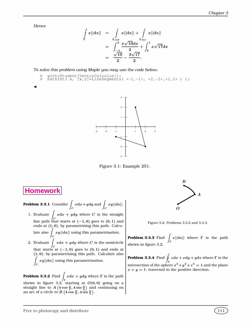
Chapter 3
Hence ZΓ
x||dx|| =
ZLAB
x||dx||+Z
LBC
x||dx||
=
Z 2
−1
x√
10dx
3+
Z 1
2x√
17dx
=
√10
2− 3√
17
2.
To solve this problem using Maple you may use the code below.
> with(Student[VectorCalculus]):> PathInt( x, [x,y]=LineSegments( <-1,-1>, <2,-2>,<1,2> ) ) ;
J
1
2
3
-1
-2
-3
1 2 3-1-2-3
b
b
b
Figure 3.1: Example 251.
Homework
Problem 3.3.1 Consider
ZC
xdx+ydy and
ZC
xy||dx||.
1. Evaluate
ZC
xdx + ydy where C is the straight
line path that starts at (−1, 0) goes to (0, 1) andends at (1, 0), by parametrising this path. Calcu-
late also
ZC
xy||dx|| using this parametrisation.
2. Evaluate
ZC
xdx + ydy where C is the semicircle
that starts at (−1, 0) goes to (0, 1) and ends at(1, 0), by parametrising this path. Calculate alsoZ
C
xy||dx|| using this parametrisation.
Problem 3.3.2 Find
ZΓ
xdx + ydy where Γ is the path
shewn in figure 3.2, starting at O(0, 0) going on a
straight line to A4 cos π
6, 4 sin π
6
and continuing on
an arc of a circle to B4 cos π
5, 4 sin π
5
.
b
O
b A
bB
Figure 3.2: Problems 3.3.2 and 3.3.3.
Problem 3.3.3 Find
ZΓ
x||dx|| where Γ is the path
shewn in figure 3.2.
Problem 3.3.4 Find
IΓ
zdx +xdy +ydz where Γ is the
intersection of the sphere x2+y2+z2 = 1 and the planex + y = 1, traversed in the positive direction.
Free to photocopy and distribute 111
Closed and Exact Forms
3.4 Closed and Exact Forms252 Lemma (Poincare Lemma) If ω is a p-differential form of continuously differentiable functions inR
n then
d(dω) = 0.
Proof: We will prove this by induction on p. For p = 0 if
ω = f(x1, x2, . . . , xn)
then
dω =nX
k=1
∂f
∂xk
dxk
and
d(dω) =nX
k=1
d
∂f
∂xk
∧ dxk
=nX
k=1
nX
j=1
∂2f
∂xj∂xk
∧ dxj
∧ dxk
=nX
1≤j≤k≤n
∂2f
∂xj∂xk
− ∂2f
∂xk∂xj
dxj ∧ dxk
= 0,
since ω is continuously differentiable and so the mixed partial derivatives are equal. Consider
now an arbitrary p-form, p > 0. Since such a form can be written as
ω =X
1≤j1≤j2≤···≤jp≤n
aj1j2...jpdxj1 ∧ dxj2 ∧ · · ·dxjp ,
where the aj1j2...jp are continuous differentiable functions in Rn, we have
dω =X
1≤j1≤j2≤···≤jp≤n
daj1j2...jp ∧ dxj1 ∧ dxj2 ∧ · · · dxjp
=X
1≤j1≤j2≤···≤jp≤n
nX
i=1
∂aj1j2...jp
∂xi
dxi
!∧ dxj1 ∧ dxj2 ∧ · · · dxjp,
it is enough to prove that for each summand
dda ∧ dxj1 ∧ dxj2 ∧ · · · dxjp
= 0.
But
dda ∧ dxj1 ∧ dxj2 ∧ · · ·dxjp
= dda ∧
dxj1 ∧ dxj2 ∧ · · · dxjp
+da ∧ d
dxj1 ∧ dxj2 ∧ · · · dxjp
= da ∧ d
dxj1 ∧ dxj2 ∧ · · · dxjp
,
since dda = 0 from the case p = 0. But an independent induction argument proves that
ddxj1 ∧ dxj2 ∧ · · · dxjp
= 0,
completing the proof.
253 Definition A differential form ω is said to be exact if there is a continuously differentiable functionF such that
dF = ω.
Free to photocopy and distribute 112
Chapter 3
254 Example The differential form
xdx + ydy
is exact, since
xdx + ydy = d
1
2(x2 + y2)
.
255 Example The differential form
ydx + xdy
is exact, since
ydx + xdy = d (xy) .
256 Example The differential formx
x2 + y2dx +
y
x2 + y2dy
is exact, sincex
x2 + y2dx +
y
x2 + y2dy = d
1
2loge(x
2 + y2)
.
Let ω = dF be an exact form. By the Poincare Lemma Theorem 252, dω = ddF = 0. A result of
Poincare says that for certain domains (called star-shaped domains) the converse is also true, that is, if
dω = 0 on a star-shaped domain then ω is exact.
257 Example Determine whether the differential form
ω =2x(1− ey)
(1 + x2)2dx +
ey
1 + x2dy
is exact.
Solution: I Assume there is a function F such that
dF = ω.
By the Chain Rule
dF =∂F
∂xdx +
∂F
∂ydy.
This demands that∂F
∂x=
2x(1− ey)
(1 + x2)2,
∂F
∂y=
ey
1 + x2.
We have a choice here of integrating either the first, or the second expression. Since integrating
the second expression (with respect to y) is easier, we find
F (x, y) =ey
1 + x2+ φ(x),
where φ(x) is a function depending only on x. To find it, we differentiate the obtained expres-
sion for F with respect to x and find
∂F
∂x= − 2xey
(1 + x2)2+ φ′(x).
Free to photocopy and distribute 113
Closed and Exact Forms
Comparing this with our first expression for∂F
∂x, we find
φ′(x) =2x
(1 + x2)2,
that is
φ(x) = − 1
1 + x2+ c,
where c is a constant. We then take
F (x, y) =ey − 1
1 + x2+ c.
J
258 Example Is there a continuously differentiable function such that
dF = ω = y2z3dx + 2xyz3dy + 3xy2z2dz ?
Solution: I We have
dω = (2yz3dy + 3y2z2dz) ∧ dx
+(2yz3dx + 2xz3dy + 6xyz2dz) ∧ dy
+(3y2z2dx + 6xyz2dy + 6xy2zdz) ∧ dz
= 0,
so this form is exact in a star-shaped domain. So put
dF =∂F
∂xdx +
∂F
∂ydy +
∂F
∂zdz = y2z3dx + 2xyz3dy + 3xy2z2dz.
Then∂F
∂x= y2z3 =⇒ F = xy2z3 + a(y, z),
∂F
∂y= 2xyz3 =⇒ F = xy2z3 + b(x, z),
∂F
∂z= 3xy2z2 =⇒ F = xy2z3 + c(x, y),
Comparing these three expressions for F , we obtain F (x, y, z) = xy2z3. J
We have the following equivalent of the Fundamental Theorem of Calculus.
259 Theorem Let U ⊆ Rn be an open set. Assume ω = dF is an exact form, and Γ a path in U with
starting point A and endpoint B. ThenZΓ
ω =
Z B
AdF = F (B)− F (A).
In particular, if Γ is a simple closed path, thenIΓ
ω = 0.
260 Example Evaluate the integral IΓ
2x
x2 + y2dx +
2y
x2 + y2dy
where Γ is the closed polygon with vertices at A = (0, 0), B = (5, 0), C = (7, 2), D = (3, 2), E = (1, 1),traversed in the order ABCDEA.
Free to photocopy and distribute 114
Chapter 3
Solution: I Observe that
d
2x
x2 + y2dx +
2y
x2 + y2dy
= − 4xy
(x2 + y2)2dy ∧ dx− 4xy
(x2 + y2)2dx ∧ dy = 0,
and so the form is exact in a start-shaped domain. By virtue of Theorem 259, the integral is 0.
J
261 Example Calculate the path integralIΓ(x2 − y)dx + (y2 − x)dy,
where Γ is a loop of x3 + y3 − 2xy = 0 traversed once in the positive sense.
Solution: I Since∂
∂y(x2 − y) = −1 =
∂
∂x(y2 − x),
the form is exact, and since this is a closed simple path, the integral is 0. J
3.5 Two-Manifolds262 Definition A 2-dimensional oriented manifold of R
2 is simply an open set (region) D ∈ R2, where the
+ orientation is counter-clockwise and the − orientation is clockwise. A general oriented 2-manifold isa union of open sets.
The region −D has opposite orientation to D andZ−D
ω = −Z
D
ω.
We will often write ZD
f(x, y)dA
where dA denotes the area element.
In this section, unless otherwise noticed, we will choose the positive orientation for the regions
considered. This corresponds to using the area form dxdy.
Let D ⊆ R2. Given a function f : D → R, the integralZ
D
fdA
is the sum of all the values of f restricted to D. In particular,ZD
dA
is the area of D.
In order to evaluate double integrals, we need the following.
263 Theorem (Fubini’s Theorem) Let D = [a; b]× [c;d], and let f : A→ R be continuous. ThenZD
fdA =
Z b
a
Z d
c
f(x, y)dy
dx =
Z d
c
Z b
a
f(x, y)dx
dy
Free to photocopy and distribute 115

Two-Manifolds
Fubini’s Theorem allows us to convert the double integral into iterated (single) integrals.
264 Example Z[0;1]×[2;3]
xydA =
Z 1
0
Z 3
2
xydy
dx
=
Z 1
0
xy2
2
32
!dx
=
Z 1
0
9x
2− 2x
dx
=
5x2
4
10
=5
4.
Notice that if we had integrated first with respect to x we would have obtained the same result:Z 3
2
Z 1
0xydx
dy =
Z 3
2
x2y
2
10
!dy
=
Z 3
2
y
2
dx
=
y2
4
32
=5
4.
Also, this integral is “factorable into x and y pieces” meaning thatZ[0;1]×[2;3]
xydA =
Z 1
0xdx
Z 3
2ydy
=
1
2
5
2
=
5
4
To solve this problem using Maple you may use the code below.> with(Student[VectorCalculus]):> int(x * y, [x,y]=Region(0..1,2..3));
265 Example We haveZ 4
3
Z 1
0(x + 2y)(2x + y) dxdy =
Z 4
3
Z 1
0(2x2 + 5xy + 2y2) dxdy
=
Z 4
3
2
3+
5
2y + 2y2
dy
=409
12.
To solve this problem using Maple you may use the code below.> with(Student[VectorCalculus]):> int((x + 2 * y) * (2 * x + y), [x,y]=Region(3..4,0..1));
In the cases when the domain of integration is not a rectangle, we decompose so that, one variableis kept constant.
266 Example Find
ZD
xy dxdy in the triangle with vertices A : (−1,−1), B : (2,−2), C : (1, 2).
Free to photocopy and distribute 116
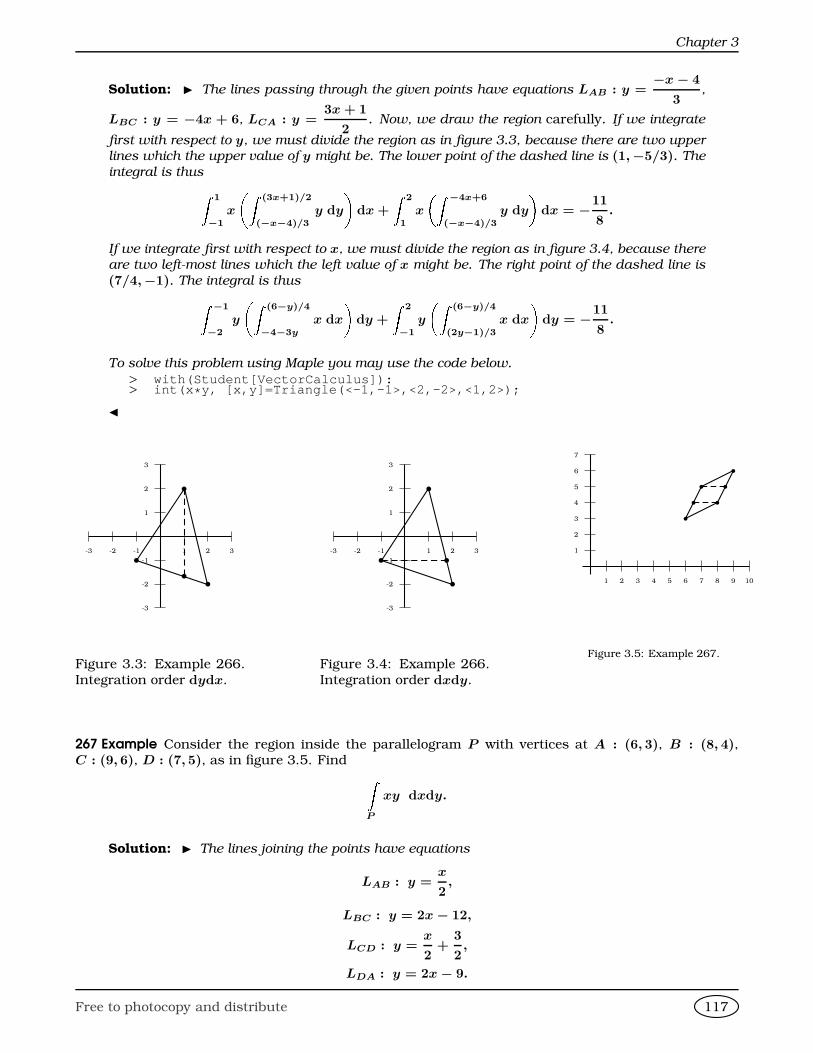
Chapter 3
Solution: I The lines passing through the given points have equations LAB : y =−x− 4
3,
LBC : y = −4x + 6, LCA : y =3x + 1
2. Now, we draw the region carefully. If we integrate
first with respect to y, we must divide the region as in figure 3.3, because there are two upper
lines which the upper value of y might be. The lower point of the dashed line is (1,−5/3). The
integral is thusZ 1
−1
x
Z (3x+1)/2
(−x−4)/3
y dy
dx +
Z 2
1
x
Z −4x+6
(−x−4)/3
y dy
dx = −11
8.
If we integrate first with respect to x, we must divide the region as in figure 3.4, because there
are two left-most lines which the left value of x might be. The right point of the dashed line is
(7/4,−1). The integral is thusZ −1
−2
y
Z (6−y)/4
−4−3y
x dx
dy +
Z 2
−1
y
Z (6−y)/4
(2y−1)/3
x dx
dy = −11
8.
To solve this problem using Maple you may use the code below.> with(Student[VectorCalculus]):> int(x * y, [x,y]=Triangle(<-1,-1>,<2,-2>,<1,2>);
J
1
2
3
-1
-2
-3
1 2 3-1-2-3b
b
b
b
Figure 3.3: Example 266.Integration order dydx.
1
2
3
-1
-2
-3
1 2 3-1-2-3b
b
b
b
Figure 3.4: Example 266.Integration order dxdy.
1
2
3
4
5
6
7
1 2 3 4 5 6 7 8 9 10
b
b
b
b
b
b
Figure 3.5: Example 267.
267 Example Consider the region inside the parallelogram P with vertices at A : (6, 3), B : (8, 4),C : (9, 6), D : (7, 5), as in figure 3.5. Find Z
P
xy dxdy.
Solution: I The lines joining the points have equations
LAB : y =x
2,
LBC : y = 2x− 12,
LCD : y =x
2+
3
2,
LDA : y = 2x− 9.
Free to photocopy and distribute 117
Two-Manifolds
The integral is thusZ 4
3
Z 2y
(y+9)/2
xy dxdy +
Z 5
4
Z (y+12)/2
(y+9)/2
xy dxdy +
Z 6
5
Z (y+12)/2
2y−3
xy dxdy =409
4.
To solve this problem using Maple you may use the code below. Notice that we have split the
parallelogram into two triangles.> with(Student[VectorCalculus]):> int(x * y, [x,y]=Triangle(<6,3>,<8,4>,<7,5>))
> + int(x * y, [x,y]=Triangle(<8,4>,<9,6>,<7,5>));
J
268 Example Find ZD
y
x2 + 1dxdy
whereD = (x, y) ∈ R
2|x ≥ 0, x2 + y2 ≤ 1.
Solution: I The integral is 0. Observe that if (x, y) ∈ D then (x,−y) ∈ D. Also, f(x,−y) =−f(x, y). J
012345
0 1 2 3 4 5
Figure 3.6: Example 269.
0
1
0 1
Figure 3.7: Example 270.
0
1
2
0 1 2
Figure 3.8: Example 271.
269 Example Find Z 4
0
Z √y
y/2ey/x dx
dy.
Solution: I We have
0 ≤ y ≤ 4,y
2≤ x ≤ √y =⇒ 0 ≤ x ≤ 2, x2 ≤ y ≤ 2x.
We then have Z 4
0
Z √y
y/2ey/xdx
dy =
Z 2
0
Z 2x
x2
ey/xdy
dx
=
Z 2
0
xey/x
2xx2
dx
=
Z 2
0(xe2 − xex) dx
= 2e2 − (2e2 − e2 + 1)
= e2 − 1
J
Free to photocopy and distribute 118
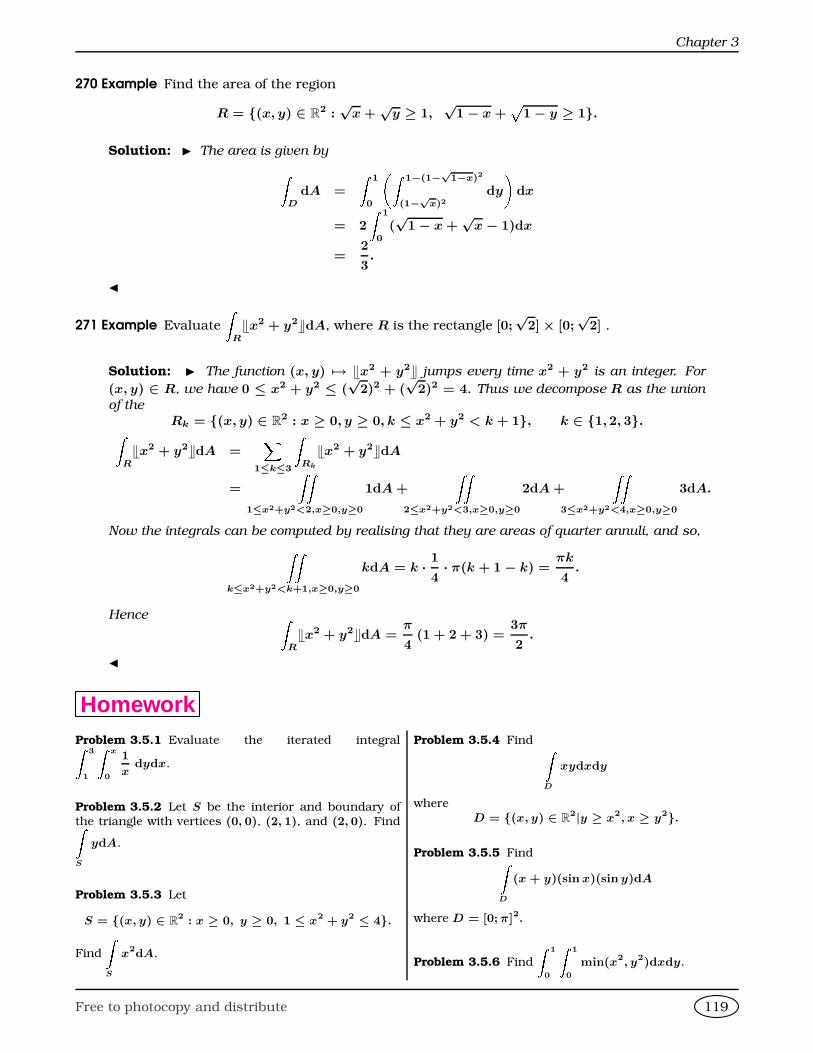
Chapter 3
270 Example Find the area of the region
R = (x, y) ∈ R2 :√
x +√
y ≥ 1,√
1− x +p
1− y ≥ 1.
Solution: I The area is given byZD
dA =
Z 1
0
Z 1−(1−√
1−x)2
(1−√x)2
dy
dx
= 2
Z 1
0(√
1− x +√
x− 1)dx
=2
3.
J
271 Example Evaluate
ZR
Tx2 + y2UdA, where R is the rectangle [0;√
2]× [0;√
2] .
Solution: I The function (x, y) 7→ Tx2 + y2U jumps every time x2 + y2 is an integer. For
(x, y) ∈ R, we have 0 ≤ x2 + y2 ≤ (√
2)2 + (√
2)2 = 4. Thus we decompose R as the union
of the
Rk = (x, y) ∈ R2 : x ≥ 0, y ≥ 0, k ≤ x2 + y2 < k + 1, k ∈ 1, 2, 3.Z
RTx2 + y2UdA =
X1≤k≤3
ZRk
Tx2 + y2UdA
=
ZZ1≤x2+y2<2,x≥0,y≥0
1dA +
ZZ2≤x2+y2<3,x≥0,y≥0
2dA +
ZZ3≤x2+y2<4,x≥0,y≥0
3dA.
Now the integrals can be computed by realising that they are areas of quarter annuli, and so,ZZk≤x2+y2<k+1,x≥0,y≥0
kdA = k · 14· π(k + 1− k) =
πk
4.
Hence ZR
Tx2 + y2UdA =π
4(1 + 2 + 3) =
3π
2.
J
HomeworkProblem 3.5.1 Evaluate the iterated integralZ 3
1
Z x
0
1
xdydx.
Problem 3.5.2 Let S be the interior and boundary ofthe triangle with vertices (0, 0), (2, 1), and (2, 0). FindZS
ydA.
Problem 3.5.3 Let
S = (x, y) ∈ R2 : x ≥ 0, y ≥ 0, 1 ≤ x2 + y2 ≤ 4.
Find
ZS
x2dA.
Problem 3.5.4 Find ZD
xydxdy
whereD = (x, y) ∈ R
2|y ≥ x2, x ≥ y2.
Problem 3.5.5 FindZD
(x + y)(sin x)(sin y)dA
where D = [0; π]2.
Problem 3.5.6 Find
Z 1
0
Z 1
0
min(x2, y2)dxdy.
Free to photocopy and distribute 119
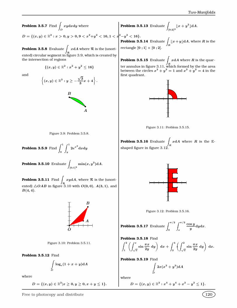
Two-Manifolds
Problem 3.5.7 Find
ZD
xydxdy where
D = (x, y) ∈ R2 : x > 0, y > 0, 9 < x2+y2 < 16, 1 < x2−y2 < 16.
Problem 3.5.8 Evaluate
ZR
xdA whereR is the (unori-
ented) circular segment in figure 3.9, which is created bythe intersection of regions
(x, y) ∈ R2 : x2 + y2 ≤ 16
and §(x, y) ∈ R
2 : y ≥ −√
3
3x + 4
ª.
b
A
bB
Figure 3.9: Problem 3.5.8.
Problem 3.5.9 Find
Z 1
0
Z 1
y
2ex2
dxdy
Problem 3.5.10 Evaluate
Z[0;1]2
min(x, y2)dA.
Problem 3.5.11 Find
ZR
xydA, where R is the (unori-
ented) 4OAB in figure 3.10 with O(0, 0), A(3, 1), and
B(4, 4).
b
O
b A
bB
Figure 3.10: Problem 3.5.11.
Problem 3.5.12 FindZD
loge(1 + x + y)dA
where
D = (x, y) ∈ R2|x ≥ 0, y ≥ 0, x + y ≤ 1.
Problem 3.5.13 Evaluate
Z[0;2]2
Tx + y2UdA.
Problem 3.5.14 Evaluate
ZR
Tx+yUdA, where R is the
rectangle [0 ; 1] × [0 ; 2].
Problem 3.5.15 Evaluate
ZR
xdA where R is the quar-
ter annulus in figure 3.11, which formed by the the areabetween the circles x2 + y2 = 1 and x2 + y2 = 4 in the
first quadrant.
Figure 3.11: Problem 3.5.15.
Problem 3.5.16 Evaluate
ZR
xdA where R is the E-
shaped figure in figure 3.12.
b b
bb
b b
bb
b b
bb
Figure 3.12: Problem 3.5.16.
Problem 3.5.17 Evaluate
Z π/2
0
Z π/2
x
cos y
ydydx.
Problem 3.5.18 FindZ 2
1
Z x
√x
sinπx
2ydy
dx +
Z 4
2
Z 2
√x
sinπx
2ydy
dx.
Problem 3.5.19 FindZD
2x(x2 + y2)dA
where
D = (x, y) ∈ R2 : x4 + y4 + x2 − y2 ≤ 1.
Free to photocopy and distribute 120
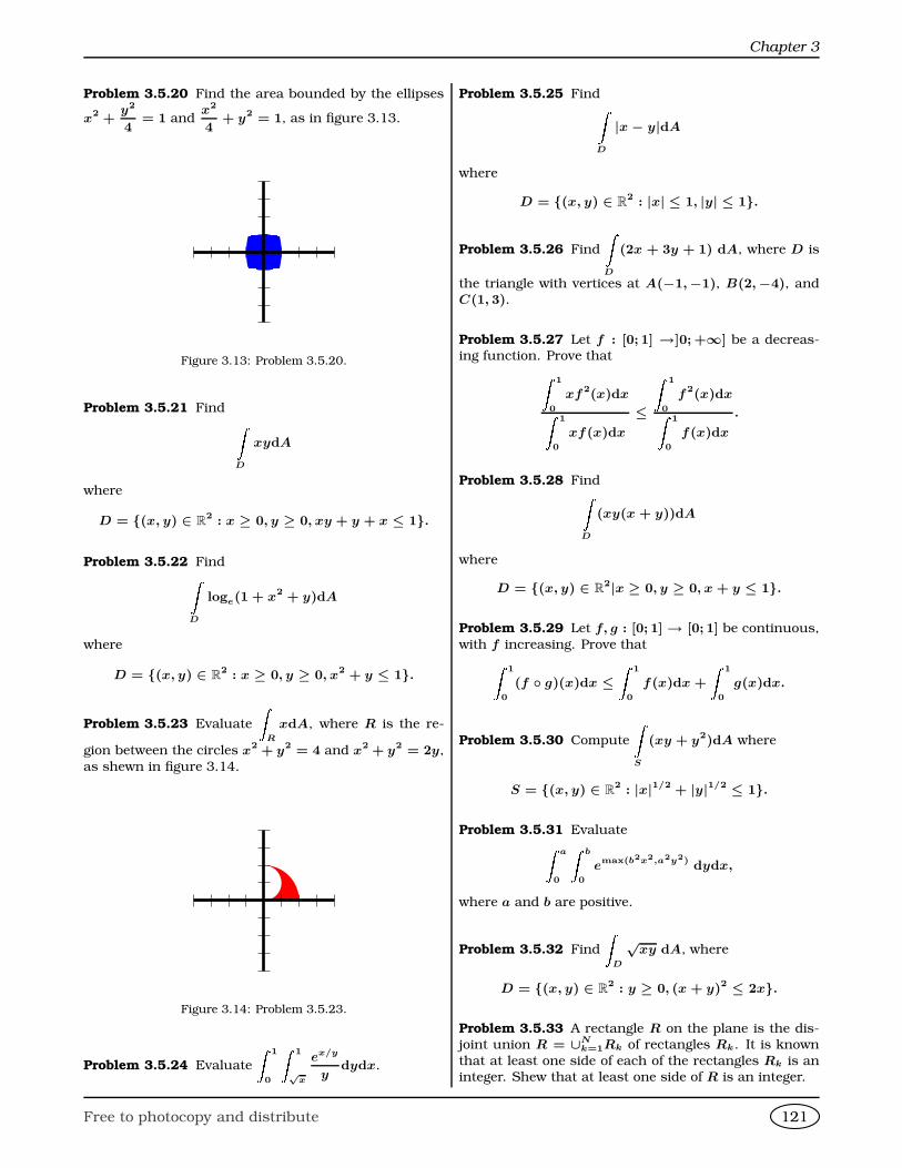
Chapter 3
Problem 3.5.20 Find the area bounded by the ellipses
x2 +y2
4= 1 and
x2
4+ y2 = 1, as in figure 3.13.
Figure 3.13: Problem 3.5.20.
Problem 3.5.21 Find ZD
xydA
where
D = (x, y) ∈ R2 : x ≥ 0, y ≥ 0, xy + y + x ≤ 1.
Problem 3.5.22 FindZD
loge(1 + x2 + y)dA
where
D = (x, y) ∈ R2 : x ≥ 0, y ≥ 0, x2 + y ≤ 1.
Problem 3.5.23 Evaluate
ZR
xdA, where R is the re-
gion between the circles x2 + y2 = 4 and x2 + y2 = 2y,
as shewn in figure 3.14.
Figure 3.14: Problem 3.5.23.
Problem 3.5.24 Evaluate
Z 1
0
Z 1
√x
ex/y
ydydx.
Problem 3.5.25 FindZD
|x − y|dA
where
D = (x, y) ∈ R2 : |x| ≤ 1, |y| ≤ 1.
Problem 3.5.26 Find
ZD
(2x + 3y + 1) dA, where D is
the triangle with vertices at A(−1,−1), B(2,−4), andC(1, 3).
Problem 3.5.27 Let f : [0; 1] →]0; +∞] be a decreas-ing function. Prove thatZ 1
0
xf2(x)dxZ 1
0
xf(x)dx
≤
Z 1
0
f2(x)dxZ 1
0
f(x)dx
.
Problem 3.5.28 FindZD
(xy(x + y))dA
where
D = (x, y) ∈ R2|x ≥ 0, y ≥ 0, x + y ≤ 1.
Problem 3.5.29 Let f, g : [0; 1]→ [0; 1] be continuous,
with f increasing. Prove thatZ 1
0
(f g)(x)dx ≤Z 1
0
f(x)dx +
Z 1
0
g(x)dx.
Problem 3.5.30 Compute
ZS
(xy + y2)dA where
S = (x, y) ∈ R2 : |x|1/2 + |y|1/2 ≤ 1.
Problem 3.5.31 EvaluateZ a
0
Z b
0
emax(b2x2,a2y2) dydx,
where a and b are positive.
Problem 3.5.32 Find
ZD
√xy dA, where
D = (x, y) ∈ R2 : y ≥ 0, (x + y)2 ≤ 2x.
Problem 3.5.33 A rectangle R on the plane is the dis-joint union R = ∪N
k=1Rk of rectangles Rk. It is known
that at least one side of each of the rectangles Rk is aninteger. Shew that at least one side of R is an integer.
Free to photocopy and distribute 121
Change of Variables
Problem 3.5.34 EvaluateZ 1
0
Z 1
0
· · ·Z 1
0
(x1x2 · · · xn)dx1dx2 . . . dxn.
Problem 3.5.35 EvaluateZ 1
0
Z 1
0
· · ·Z 1
0
(x1 + x2 + · · ·+ xn) dx1dx2 . . . dxn.
Problem 3.5.36 Let I be the rectangle [1; 2]× [1; 2] andlet f, g be continuous functions f, g : [1; 2] → [1; 2]such that f(x) ≤ g(x). Demonstrate thatZ
I
(g(y)− f(x)) dxdy ≥ 0.
Problem 3.5.37 Find
Z 1
0
Z 1
0
xydxdy. Then demon-
strate that
Z 1
0
x − 1
log xdx = log 2.
Problem 3.5.38 EvaluateZ 4
0
Z √4−y
0
p12x − x3dxdy.
Problem 3.5.39 Evaluate
Z 2
0
Z 2
y
yp
1 + x3dxdy.
Problem 3.5.40 Evaluate
Z 1
0
Z 1
y
xy√1 + x4
dxdy.
Problem 3.5.41 FindZD
1
(x + y)4dA
where
D = (x, y) ∈ R2|x ≥ 1, y ≥ 1, x + y ≤ 4.
Problem 3.5.42 Prove thatZ +∞
0
Z +∞
2x
xe−y sin y
y2dydx =
1
16.
Problem 3.5.43 Prove thatZ 1
0
Z y
y2
y
xp
x2 + y2dxdy = log(1 +
√2).
Problem 3.5.44 Prove thatZ 1
0
Z 1
0
x − y
(x + y)3dydx =
1
2= −
Z 1
0
Z 1
0
x − y
(x + y)3dxdy.
Is this a contradiction to Fubini’s Theorem?
Problem 3.5.45 Find ZD
xdA
where
D = (x, y) ∈ R2|y ≥ 0, x−y+1 ≥ 0, x+2y−4 ≤ 0.
Problem 3.5.46 Evaluate
limn→+∞
Z 1
0
Z 1
0
· · ·Z 1
0
cos2 π
2n(x1 + x2 + · · · + xn)
dx1 dx2 . . . dxn
Problem 3.5.47 Let f, g be continuous functions in the
interval [a; b]. Prove that
1
2
Z b
a
Z b
a
det
f(x) g(x)
f(y) g(y)
2
dx
!dy
equalsZ b
a
(f(x))2dx
Z b
a
(g(x))2dx
−Z b
a
(f(x)g(x))dx
2
.
This is an integral analogue of Lagrange’s Identity. De-
duce Cauchy’s Inequality for integrals,Z b
a
(f(x)g(x))dx
2
≤Z b
a
(f(x))2dx
Z b
a
(g(x))2dx
.
Problem 3.5.48 Let a ∈ R, n ∈ N, a > 0, n > 0. Letf : [0; a]→ R be continuous. Prove thatZ a
0
Z x1
0
· · ·Z xn−2
0
Z xn−1
0
(f(x1)f(x2) · · · f(xn))dxndxn−1 . . . dx2dx
equals
1
n!
Z a
0
f(x)dx
n
.
3.6 Change of VariablesWe now perform a multidimensional analogue of the change of variables theorem in one variable.
272 Theorem Let (D, ∆) ∈ (Rn)2 be open, bounded sets in Rn with volume and let g : ∆ → D be a
continuously differentiable bijective mapping such that det g′(u) 6= 0, and both |det g′(u)|, 1
|det g′(u)|
Free to photocopy and distribute 122
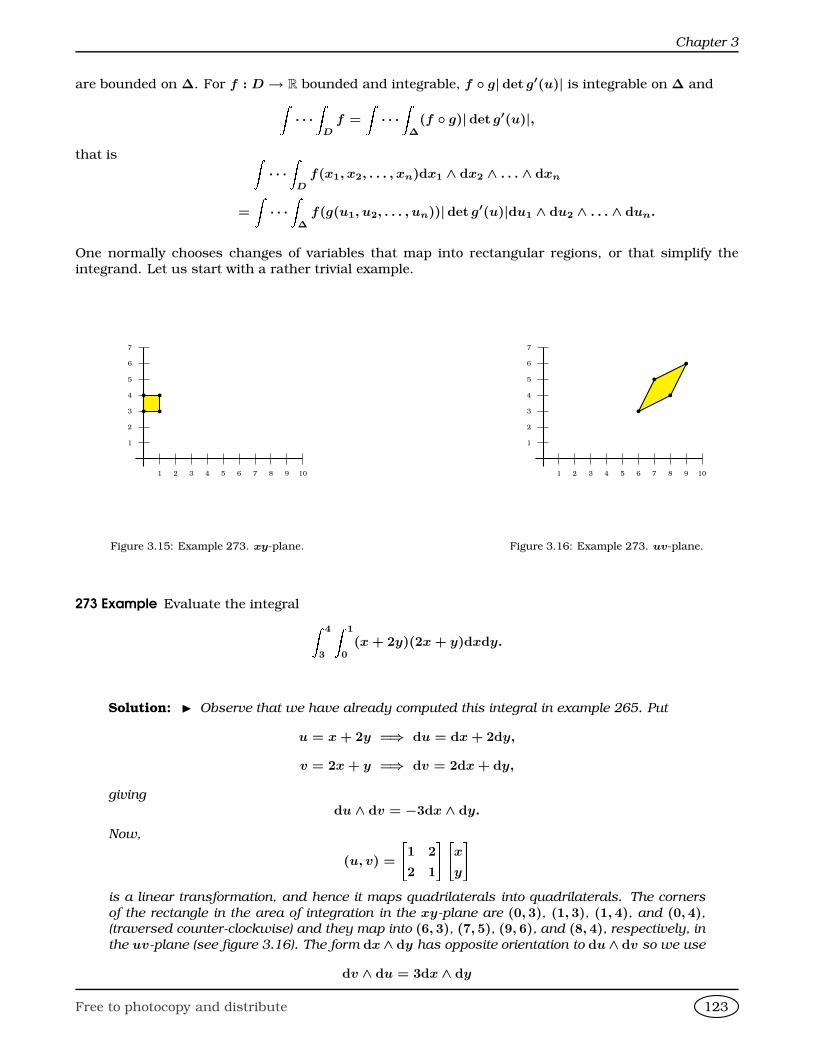
Chapter 3
are bounded on ∆. For f : D → R bounded and integrable, f g| det g′(u)| is integrable on ∆ andZ· · ·Z
Df =
Z· · ·Z∆
(f g)| det g′(u)|,
that is Z· · ·Z
Df(x1, x2, . . . , xn)dx1 ∧ dx2 ∧ . . . ∧ dxn
=
Z· · ·Z∆
f(g(u1, u2, . . . , un))|det g′(u)|du1 ∧ du2 ∧ . . . ∧ dun.
One normally chooses changes of variables that map into rectangular regions, or that simplify theintegrand. Let us start with a rather trivial example.
1
2
3
4
5
6
7
1 2 3 4 5 6 7 8 9 10
b
b b
b
Figure 3.15: Example 273. xy-plane.
1
2
3
4
5
6
7
1 2 3 4 5 6 7 8 9 10
b
b
b
b
Figure 3.16: Example 273. uv-plane.
273 Example Evaluate the integral Z 4
3
Z 1
0
(x + 2y)(2x + y)dxdy.
Solution: I Observe that we have already computed this integral in example 265. Put
u = x + 2y =⇒ du = dx + 2dy,
v = 2x + y =⇒ dv = 2dx + dy,
giving
du ∧ dv = −3dx ∧ dy.
Now,
(u, v) =
"1 2
2 1
# "x
y
#is a linear transformation, and hence it maps quadrilaterals into quadrilaterals. The corners
of the rectangle in the area of integration in the xy-plane are (0, 3), (1, 3), (1, 4), and (0, 4),(traversed counter-clockwise) and they map into (6, 3), (7, 5), (9, 6), and (8, 4), respectively, in
the uv-plane (see figure 3.16). The form dx∧ dy has opposite orientation to du∧ dv so we use
dv ∧ du = 3dx ∧ dy
Free to photocopy and distribute 123
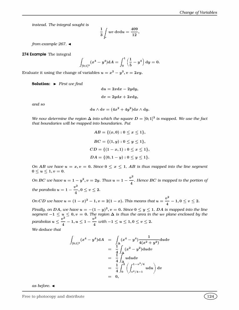
Change of Variables
instead. The integral sought is1
3
ZP
uv dvdu =409
12,
from example 267. J
274 Example The integral Z[0;1]2
(x4 − y4)dA =
Z 1
0
1
5− y4
dy = 0.
Evaluate it using the change of variables u = x2 − y2, v = 2xy.
Solution: I First we find
du = 2xdx− 2ydy,
dv = 2ydx + 2xdy,
and so
du ∧ dv = (4x2 + 4y2)dx ∧ dy.
We now determine the region ∆ into which the square D = [0; 1]2 is mapped. We use the fact
that boundaries will be mapped into boundaries. Put
AB = (x, 0) : 0 ≤ x ≤ 1,
BC = (1, y) : 0 ≤ y ≤ 1,
CD = (1− x, 1) : 0 ≤ x ≤ 1,
DA = (0, 1− y) : 0 ≤ y ≤ 1.
On AB we have u = x, v = 0. Since 0 ≤ x ≤ 1, AB is thus mapped into the line segment
0 ≤ u ≤ 1, v = 0.
On BC we have u = 1− y2, v = 2y. Thus u = 1− v2
4. Hence BC is mapped to the portion of
the parabola u = 1− v2
4, 0 ≤ v ≤ 2.
On CD we have u = (1− x)2 − 1, v = 2(1− x). This means that u =v2
4− 1, 0 ≤ v ≤ 2.
Finally, on DA, we have u = −(1 − y)2, v = 0. Since 0 ≤ y ≤ 1, DA is mapped into the line
segment −1 ≤ u ≤ 0, v = 0. The region ∆ is thus the area in the uv plane enclosed by the
parabolas u ≤ v2
4− 1, u ≤ 1− v2
4with −1 ≤ u ≤ 1, 0 ≤ v ≤ 2.
We deduce that Z[0;1]2
(x4 − y4)dA =
Z∆
(x4 − y4)1
4(x2 + y2)dudv
=1
4
Z∆
(x2 − y2)dudv
=1
4
Z∆
ududv
=1
4
Z 2
0
Z 1−v2/4
v2/4−1
udu
dv
= 0,
as before. J
Free to photocopy and distribute 124
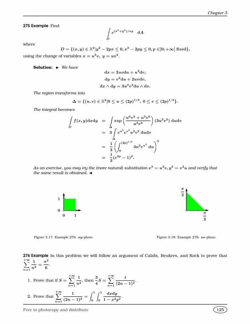
Chapter 3
275 Example Find ZD
e(x3+y3)/xy dA
whereD = (x, y) ∈ R
2|y2 − 2px ≤ 0, x2 − 2py ≤ 0, p ∈]0;+∞[ fixed,using the change of variables x = u2v, y = uv2.
Solution: I We have
dx = 2uvdu + u2dv,
dy = v2du + 2uvdv,
dx ∧ dy = 3u2v2du ∧ dv.
The region transforms into
∆ = (u, v) ∈ R2|0 ≤ u ≤ (2p)1/3, 0 ≤ v ≤ (2p)1/3.
The integral becomesZD
f(x, y)dxdy =
Z∆
exp
u6v3 + u3v6
u3v3
(3u2v2) dudv
= 3
Z∆
eu3
ev3
u2v2 dudv
=1
3
Z (2p)1/3
0
3u2eu3
du
!2
=1
3(e2p − 1)2.
As an exercise, you may try the (more natural) substitution x3 = u2v, y3 = v2u and verify that
the same result is obtained. J
0
1
0 1
b b
bb
Figure 3.17: Example 276. xy-plane.
b b
b
π
2
π
2
Figure 3.18: Example 276. uv-plane.
276 Example In this problem we will follow an argument of Calabi, Beukers, and Kock to prove that+∞Xn=1
1
n2=
π2
6.
1. Prove that if S =
+∞Xn=1
1
n2, then
3
4S =
+∞Xn=1
1
(2n− 1)2.
2. Prove that
+∞Xn=1
1
(2n− 1)2=
Z 1
0
Z 1
0
dxdy
1− x2y2.
Free to photocopy and distribute 125
Change of Variables
3. Use the change of variables x =sin u
cos v, y =
sin v
cos uin order to evaluate
Z 1
0
Z 1
0
dxdy
1− x2y2.
Solution: I
1. Observe that the sum of the even terms is
+∞Xn=1
1
(2n)2=
1
4
+∞Xn=1
1
n2=
1
4S,
a quarter of the sum, hence the sum of the odd terms must be three quarters of the sum,3
4S.
2. Observe that
1
2n− 1=
Z 1
0x2n−2dx =⇒
1
2n− 1
2
=
Z 1
0x2n−2dx
Z 1
0y2n−2dy
=
Z 1
0
Z 1
0(xy)2n−2dxdy.
Thus
+∞Xn=1
1
(2n− 1)2=
+∞Xn=1
Z 1
0
Z 1
0(xy)2n−2dxdy =
Z 1
0
Z 1
0
+∞Xn=1
(xy)2n−2dxdy =
Z 1
0
Z 1
0
dxdy
1− x2y2,
as claimed.3
3. If x =sin u
cos v, y =
sin v
cos u, then
dx = (cos u)(sec v)du+(sin u)(sec v)(tan v)dv, dy = (sec u)(tan u)(sin v)du+(sec u)(cos v)dv,
from where
dx ∧ dy = du ∧ dv − (tan2 u)(tan2 v)du ∧ dv =1− (tan2 u)(tan2 v)
du ∧ dv.
Also,
1− x2y2 = 1− sin2 v
cos2 v· sin2 v
cos2 u= 1− (tan2 u)(tan2 v).
This givesdxdy
1− x2y2= dudv.
We now have to determine the region that the transformation x =sin u
cos v, y =
sin v
cos uforms
in the uv-plane. Observe that
u = arctan x
Ê1− y2
1− x2, v = arctan y
s1− x2
1− y2.
This means that the square in the xy-plane in figure 3.17 is transformed into the triangle
in the uv-plane in figure 3.18.
We deduce,Z 1
0
Z 1
0
dxdy
1− x2y2=
Z π/2
0
Z π/2−v
0dudv =
Z π/2
0(π/2− v) dv =
π
2v − v2
2
π/2
0=
π2
4−π2
8=
π2
8.
Finally,3
4S =
π2
8=⇒ S =
π2
6.
J
3This exchange of integral and sum needs justification. We will accept it for our purposes.
Free to photocopy and distribute 126
Chapter 3
Homework
Problem 3.6.1 Let D′ = (u, v) ∈ R2 : u ≤ 1,−u ≤ v ≤ u. Consider
Φ :R
2 → R2
(u, v) 7→
u + v
2,u − v
2
.
➊ Find the image of Φ on D′, that is, find D = Φ(D′).
➋ Find ZD
(x + y)2ex2−y2
dA.
Problem 3.6.2 Using the change of variables x = u2 − v2, y = 2uv, u ≥ 0, v ≥ 0, evaluate
ZR
px2 + y2dA,
where
R = (x, y) ∈ R2 : −1 ≤ x ≤ 1, 0 ≤ y ≤ 2
È1− |x|
Problem 3.6.3 Using the change of variables u = x − y and v = x + y, evaluate
ZR
x − y
x + ydA, where R is the
square with vertices at (0, 2), (1, 1), (2, 2), (1, 3).
Problem 3.6.4 Find
ZD
f(x, y)dA where
D = (x, y) ∈ R2|a ≤ xy ≤ b, y ≥ x ≥ 0, y2 − x2 ≤ 1, (a, b) ∈ R
2, 0 < a < b
and f(x, y) = y4 − x4 by using the change of variables u = xy, v = y2 − x2.
Problem 3.6.5 Use the following steps (due to Tom Apostol) in order to prove that
∞Xn=1
1
n2=
π2
6.
➊ Use the series expansion
1
1− t= 1 + t + t2 + t3 + · · · |t| < 1,
in order to prove (formally) that Z 1
0
Z 1
0
dxdy
1− xy=
∞Xn=1
1
n2.
➋ Use the change of variables u = x + y, v = x − y to shew thatZ 1
0
Z 1
0
dxdy
1− xy= 2
Z 1
0
Z u
−u
dv
4− u2 + v2
du + 2
Z 2
1
Z 2−u
u−2
dv
4− u2 + v2
du.
➌ Shew that the above integral reduces to
2
Z 1
0
2√4− u2
arctanu√
4− u2du + 2
Z 2
1
2√4− u2
arctan2− u√4− u2
du.
➍ Finally, prove that the above integral isπ2
6by using the substitution θ = arcsin
u
2.
Free to photocopy and distribute 127
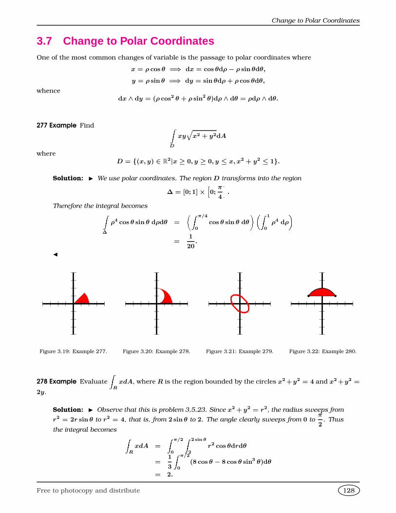
Change to Polar Coordinates
3.7 Change to Polar CoordinatesOne of the most common changes of variable is the passage to polar coordinates where
x = ρ cos θ =⇒ dx = cos θdρ− ρ sin θdθ,
y = ρ sin θ =⇒ dy = sin θdρ + ρ cos θdθ,
whencedx ∧ dy = (ρ cos2 θ + ρ sin2 θ)dρ ∧ dθ = ρdρ ∧ dθ.
277 Example Find ZD
xyÈ
x2 + y2dA
whereD = (x, y) ∈ R
2|x ≥ 0, y ≥ 0, y ≤ x, x2 + y2 ≤ 1.
Solution: I We use polar coordinates. The region D transforms into the region
∆ = [0; 1]×h0;
π
4
i.
Therefore the integral becomesZ∆
ρ4 cos θ sin θ dρdθ =
Z π/4
0cos θ sin θ dθ
Z 1
0ρ4 dρ
=
1
20.
J
Figure 3.19: Example 277. Figure 3.20: Example 278. Figure 3.21: Example 279.
b b
Figure 3.22: Example 280.
278 Example Evaluate
ZR
xdA, where R is the region bounded by the circles x2 +y2 = 4 and x2 +y2 =
2y.
Solution: I Observe that this is problem 3.5.23. Since x2 + y2 = r2, the radius sweeps from
r2 = 2r sin θ to r2 = 4, that is, from 2 sin θ to 2. The angle clearly sweeps from 0 toπ
2. Thus
the integral becomes ZR
xdA =
Z π/2
0
Z 2 sin θ
2
r2 cos θdrdθ
=1
3
Z π/2
0
(8 cos θ − 8 cos θ sin3 θ)dθ
= 2.
Free to photocopy and distribute 128
Chapter 3
J
279 Example Find
ZD
e−x2−xy−y2
dA, where
D = (x, y) ∈ R2 : x2 + xy + y2 ≤ 1.
Solution: I Completing squares
x2 + xy + y2 =x +
y
2
2
+
√3y
2
2
.
Put U = x +y
2, V =
√3y
2. The integral becomesZ
x2+xy+y2≤1e−x2−xy−y2
dxdy =2√3
ZU2+V 2≤1
e−(U2+V 2)dUdV.
Passing to polar coordinates, the above equals
2√3
Z 2π
0
Z 1
0
ρe−ρ2
dρdθ =2π√
3(1− e−1).
J
280 Example Evaluate
ZR
1
(x2 + y2)3/2dA over the region
¦(x, y) ∈ R
2 : x2 + y2 ≤ 4, y ≥ 1©
(figure 3.22).
Solution: I The radius sweeps from r =1
sin θto r = 2. The desired integral isZ
R
1
(x2 + y2)3/2dA =
Z 5π/6
π/6
Z 2
csc θ
1
r2drdθ
=
Z 5π/6
π/6
sin θ − 1
2
dθ
=√
3− π
3.
J
281 Example Evaluate
ZR(x3 + y3)dA where R is the region bounded by the ellipse
x2
a2+
y2
b2= 1 and
the first quadrant, a > 0 and b > 0.
Solution: I Put x = ar cos θ, y = br sin θ. Then
x = ar cos θ =⇒ dx = a cos θdr − ar sin θdθ,
y = br sin θ =⇒ dy = b sin θdr + br cos θdθ,
whence
dx ∧ dy = (abr cos2 θ + abr sin2 θ)dr ∧ dθ = abrdr ∧ dθ.
Observe that on the ellipse
x2
a2+
y2
b2= 1 =⇒ a2r2 cos2 θ
a2+
b2r2 sin2 θ
b2= 1 =⇒ r = 1.
Free to photocopy and distribute 129
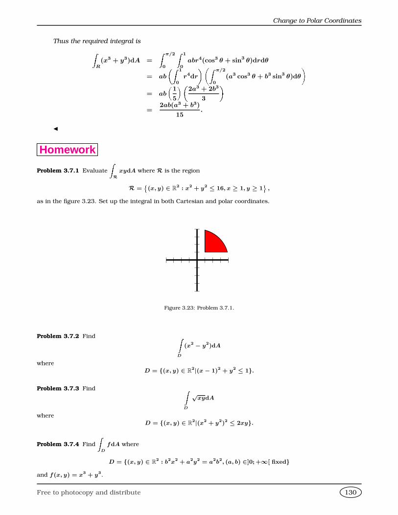
Change to Polar Coordinates
Thus the required integral isZR(x3 + y3)dA =
Z π/2
0
Z 1
0abr4(cos3 θ + sin3 θ)drdθ
= ab
Z 1
0r4dr
Z π/2
0(a3 cos3 θ + b3 sin3 θ)dθ
= ab
1
5
2a3 + 2b3
3
=
2ab(a3 + b3)
15.
J
Homework
Problem 3.7.1 Evaluate
ZR
xydA where R is the region
R =(x, y) ∈ R
2 : x2 + y2 ≤ 16, x ≥ 1, y ≥ 1
,
as in the figure 3.23. Set up the integral in both Cartesian and polar coordinates.
Figure 3.23: Problem 3.7.1.
Problem 3.7.2 Find ZD
(x2 − y2)dA
where
D = (x, y) ∈ R2|(x − 1)2 + y2 ≤ 1.
Problem 3.7.3 Find ZD
√xydA
where
D = (x, y) ∈ R2|(x2 + y2)2 ≤ 2xy.
Problem 3.7.4 Find
ZD
fdA where
D = (x, y) ∈ R2 : b2x2 + a2y2 = a2b2, (a, b) ∈]0;+∞[ fixed
and f(x, y) = x3 + y3.
Free to photocopy and distribute 130
Chapter 3
Problem 3.7.5 Let a > 0 and b > 0. Prove thatZR
ra2b2 − a2y2 − b2x2
a2b2 + a2y2 + b2x2dA =
πab(π − 2)
8,
where R is the region bounded by the ellipsex2
a2+
y2
b2= 1 and the first quadrant.
Problem 3.7.6 Prove that ZR
ypx2 + y2
dxdy =√
2− 1,
where
R = (x, y) ∈ R2 : 0 < x < 1, o < y < x2.
Problem 3.7.7 Prove that the ellipse
(x − 2y + 3)2 + (3x + 4y − 1)2 = 4
bounds an area of2π
5.
Problem 3.7.8 Find ZD
px2 + y2dA
whereD = (x, y) ∈ R
2|x ≥ 0, y ≥ 0, x2 + y2 ≤ 1, x2 + y2 − 2y ≥ 0.
Problem 3.7.9 Find
ZD
fdA where
D = (x, y) ∈ R2|y ≥ 0, x2 + y2 − 2x ≤ 0
and f(x, y) = x2y.
Problem 3.7.10 Let D = (x, y) ∈ R2 : x ≥ 1, x2 + y2 ≤ 4. Find
ZD
xdA.
Problem 3.7.11 Find
ZD
fdA where
D = (x, y) ∈ R2|x ≥ 1, x2 + y2 − 2x ≤ 0
and f(x, y) =1
(x2 + y2)2.
Problem 3.7.12 LetD = (x, y) ∈ R
2 : x2 + y2 − y ≤ 0, x2 + y2 − x ≤ 0.Find the integral Z
D
(x + y)2dA.
Problem 3.7.13 Let D = (x, y) ∈ R2|y ≤ x2 + y2 ≤ 1. ComputeZ
D
dA
(1 + x2 + y2)2.
Problem 3.7.14 Evaluate Z(x,y)∈R2:x≥0,y≥0,x4+y4≤1
x3y3p
1− x4 − y4 dA
using x2 = ρ cos θ, y2 = ρ sin θ.
Free to photocopy and distribute 131
Three-Manifolds
Problem 3.7.15 William Thompson (Lord Kelvin) is credited to have said: “A mathematician is someone to whomZ +∞
0
e−x2
dx =
√π
2
is as obvious as twice two is four to you. Liouville was a mathematician.” Prove thatZ +∞
0
e−x2
dx =
√π
2
by following these steps.
➊ Let a > 0 be a real number and put Da = (x, y) ∈ R2|x2 + y2 ≤ a2. Find
Ia =
ZDa
e−(x2+y2) dxdy.
➋ Let a > 0 be a real number and put ∆a = (x, y) ∈ R2||x| ≤ a, |y| ≤ a. Let
Ja =
Z∆a
e−(x2+y2) dxdy.
Prove that
Ia ≤ Ja ≤ Ia√
2.
➌ Deduce that Z +∞
0
e−x2
dx =
√π
2.
Problem 3.7.16 Let D = (x, y) ∈ R2 : 4 ≤ x2 + y2 ≤ 16 and f(x, y) =
1
x2 + xy + y2. Find
ZD
f(x, y)dA.
Problem 3.7.17 Prove that every closed convex region in the plane of area ≥ π has two points which are two units
apart.
Problem 3.7.18 In the xy-plane, if R is the set of points inside and on a convex polygon, let D(x, y) be thedistance from (x, y) to the nearest point R. Show thatZ +∞
−∞
Z +∞
−∞e−D(x,y) dxdy = 2π + L + A,
where L is the perimeter of R and A is the area of R.
3.8 Three-Manifolds282 Definition A 3-dimensional oriented manifold of R
3 is simply an open set (body) V ∈ R3, where the
+ orientation is in the direction of the outward pointing normal to the body, and the − orientation isin the direction of the inward pointing normal to the body. A general oriented 3-manifold is a union ofopen sets.
The region −M has opposite orientation to M andZ−M
ω = −Z
M
ω.
We will often write ZM
fdV
where dV denotes the volume element.
Free to photocopy and distribute 132
Chapter 3
In this section, unless otherwise noticed, we will choose the positive orientation for the regions
considered. This corresponds to using the volume form dx ∧ dy ∧ dz.
Let V ⊆ R3. Given a function f : V → R, the integralZ
V
fdV
is the sum of all the values of f restricted to V . In particular,ZV
dV
is the oriented volume of V .
283 Example Find Z[0;1]3
x2yexyz dV.
Solution: I The integral isZ 1
0
Z 1
0
Z 1
0x2yexyz dz
dy
dx =
Z 1
0
Z 1
0x(exy − 1) dy
dx
=
Z 1
0(ex − x− 1)dx
= e− 5
2.
J
284 Example Find
ZR
z dV if
R = (x, y, z) ∈ R3|x ≥ 0, y ≥ 0, z ≥ 0,
√x +√
y +√
z ≤ 1.
Solution: I The integral isZR
zdxdydz =
Z 1
0
z
Z (1−√z)2
0
Z (1−√z−√
x)2
0
dy
dx
dz
=
Z 1
0z
Z (1−√z)2
0(1−
√z −√
x)2dx
dz
=1
6
Z 1
0z(1 −
√z)4 dz
=1
840.
J
285 Example Prove that ZV
xdV =a2bc
24,
where V is the tetrahedron
V =n(x, y, z) ∈ R
3 : x ≥ 0, y ≥ 0, z ≥ 0,x
a+
y
b+
z
c≤ 1
o.
Free to photocopy and distribute 133
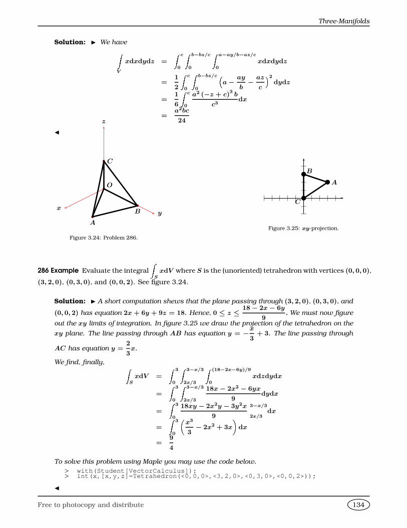
Three-Manifolds
Solution: I We haveZV
xdxdydz =
Z c
0
Z b−bz/c
0
Z a−ay/b−az/c
0xdxdydz
=1
2
Z c
0
Z b−bz/c
0
a− ay
b− az
c
2
dydz
=1
6
Z c
0
a2 (−z + c)3
b
c3dx
=a2bc
24
J
xy
z
b O
b
A
b
B
b C
Figure 3.24: Problem 286.
b A
b B
bC
Figure 3.25: xy-projection.
286 Example Evaluate the integral
ZS
xdV where S is the (unoriented) tetrahedron with vertices (0, 0, 0),
(3, 2, 0), (0, 3, 0), and (0, 0, 2). See figure 3.24.
Solution: I A short computation shews that the plane passing through (3, 2, 0), (0, 3, 0), and
(0, 0, 2) has equation 2x + 6y + 9z = 18. Hence, 0 ≤ z ≤ 18− 2x− 6y
9. We must now figure
out the xy limits of integration. In figure 3.25 we draw the projection of the tetrahedron on the
xy plane. The line passing through AB has equation y = −x
3+ 3. The line passing through
AC has equation y =2
3x.
We find, finally, ZS
xdV =
Z 3
0
Z 3−x/3
2x/3
Z (18−2x−6y)/9
0xdzdydx
=
Z 3
0
Z 3−x/3
2x/3
18x− 2x2 − 6yx
9dydx
=
Z 3
0
18xy − 2x2y − 3y2x
9
3−x/3
2x/3dx
=
Z 3
0
x3
3− 2x2 + 3x
dx
=9
4
To solve this problem using Maple you may use the code below.
> with(Student[VectorCalculus]):> int(x,[x,y,z]=Tetrahedron(<0,0,0>,<3,2,0>,<0,3,0>,< 0,0,2>));
J
Free to photocopy and distribute 134
Chapter 3
287 Example Evaluate
ZR
xyzdV , where R is the solid formed by the intersection of the parabolic
cylinder z = 4− x2, the planes z = 0, y = x, and y = 0. Use the following orders of integration:
1. dzdxdy
2. dxdydz
Solution: I We must find the projections of the solid on the the coordinate planes.
1. With the order dzdxdy, the limits of integration of z can only depend, if at all, on x and y.
Given an arbitrary point in the solid, its lowest z coordinate is 0 and its highest one is on
the cylinder, so the limits for z are from z = 0 to z = 4− x2. The projection of the solid on
the xy-plane is the area bounded by the lines y = x, x = 2, and the x and y axes.Z 2
0
Z y
0
Z 4−x2
0xyzdzdxdy =
1
2
Z 2
0
Z y
0xy(4− x2)2dxdy
=1
2
Z 2
0
Z y
0y(16x− 8x3 + x5)dxdy
=
Z 2
0
4y3 − y5 +
y7
12
dy
= 8.
2. With the order dxdydz, the limits of integration of x can only depend, if at all, on y and z.
Given an arbitrary point in the solid, x sweeps from the plane to x = 2, so the limits for
x are from x = y to x =√
4− z. The projection of the solid on the yz-plane is the area
bounded by z = 4− y2, and the z and y axes.Z 4
0
Z √4−z
0
Z 2
y
xyzdxdydz =1
2
Z 4
0
Z √4−z
0
(4y − y3)zdydz
=
Z 4
0
2z − z3
8
dz
= 8.
J
Homework
Problem 3.8.1 Compute
ZE
zdV where E is the region in the first octant bounded by the planes y + z = 1 and
x + z = 1.
Problem 3.8.2 Consider the solid S in the first octant, bounded by the parabolic cylinder z = 2 − x2
2and the
planes z = 0, y = x, and y = 0. Prove that
ZS
xyz =2
3first by integrating in the order dzdydx, and then by
integrating in the order dydxdz.
Problem 3.8.3 Evaluate the integrals
ZR
1dV and
ZR
xdV , where R is the tetrahedron with vertices at (0, 0, 0),
(1, 1, 1), (1, 0, 0), and (0, 0, 1).
Problem 3.8.4 Compute
ZE
xdV where E is the region in the first octant bounded by the plane y = 3z and the
cylinder x2 + y2 = 9.
Free to photocopy and distribute 135
Change of Variables
Problem 3.8.5 Find
ZD
dV
(1 + x2z2)(1 + y2z2)where
D = (x, y, z) ∈ R3 : 0 ≤ x ≤ 1, 0 ≤ y ≤ 1, z ≥ 0.
3.9 Change of Variables288 Example Find Z
R
(x + y + z)(x + y − z)(x − y − z)dV,
where R is the tetrahedron bounded by the planes x + y + z = 0, x + y − z = 0, x − y − z = 0, and2x− z = 1.
Solution: I We make the change of variables
u = x + y + z =⇒ du = dx + dy + dz,
v = x + y − z =⇒ dv = dx + dy − dz,
w = x− y − z =⇒ dw = dx− dy − dz.
This gives
du ∧ dv ∧ dw = −4dx ∧ dy ∧ dz.
These forms have opposite orientations, so we choose, say,
du ∧ dw ∧ dv = 4dx ∧ dy ∧ dz
which have the same orientation. Also,
2x− z = 1 =⇒ u + v + 2w = 2.
The tetrahedron in the xyz-coordinate frame is mapped into a tetrahedron bounded by u = 0,
v = 0, u + v + 2w = 1 in the uvw-coordinate frame. The integral becomes
1
4
Z 2
0
Z 1−v/2
0
Z 2−v−2w
0uvw dudwdv =
1
180.
Consider a transformation to cylindrical coordinates
(x, y, z) = (ρ cos θ, ρ sin θ, z).
From what we know about polar coordinates
dx ∧ dy = ρdρ ∧ dθ.
Since the wedge product of forms is associative,
dx ∧ dy ∧ dz = ρdρ ∧ dθ ∧ dz.
J
289 Example Find
ZR
z2dxdydz if
R = (x, y, z) ∈ R3|x2 + y2 ≤ 1, 0 ≤ z ≤ 1.
Free to photocopy and distribute 136
Chapter 3
Solution: I The region of integration is mapped into
∆ = [0; 2π]× [0; 1]× [0; 1]
through a cylindrical coordinate change. The integral is thereforeZR
f(x, y, z)dxdydz =
Z 2π
0dθ
Z 1
0ρ dρ
Z 1
0z2 dz
=
π
3.
J
290 Example Evaluate
ZD
(x2 + y2)dxdydz over the first octant region bounded by the cylinders x2 +
y2 = 1 and x2 + y2 = 4 and the planes z = 0, z = 1, x = 0, x = y.
Solution: I The integral is Z 1
0
Z π/2
π/4
Z 2
1ρ3dρdθdz =
15π
16.
J
291 Example Three long cylinders of radius R intersect at right angles. Find the volume of their inter-section.
Solution: I Let V be the desired volume. By symmetry, V = 24V ′, where
V ′ =
ZD′
dxdydz,
D′ = (x, y, z) ∈ R3 : 0 ≤ y ≤ x, 0 ≤ z, x2 + y2 ≤ R2, y2 + z2 ≤ R2, z2 + x2 ≤ R2.
In this case it is easier to integrate with respect to z first. Using cylindrical coordinates
∆′ =n(θ, ρ, z) ∈
h0;
π
4
i× [0; R]× [0;+∞[, 0 ≤ z ≤
ÈR2 − ρ2 cos2 θ
o.
Now,
V ′ =
Z π/4
0
Z R
0
Z √R2−ρ2 cos2 θ
0dz
!ρdρ
!dθ
=
Z π/4
0
Z R
0ρÈ
R2 − ρ2 cos2 θdρ
dθ
=
Z π/4
0− 1
3 cos2 θ
(R2 − ρ2 cos2 θ)3/2
R0
dθ
=R3
3
Z π/4
0
1− sin3 θ
cos2 θdθ
=
u = cos θR3
3
[tan θ]
π/40 +
Z √2
2
1
1− u2
u2du
!=
R3
3
1−
u−1 + u
√2
2
1
=
√2− 1√
2R3.
Finally
V = 16V ′ = 8(2−√
2)R3.
J
Free to photocopy and distribute 137
Change of Variables
Consider now a change to spherical coordinates
x = ρ cos θ sin φ, y = ρ sin θ sin φ, z = ρ cos φ.
We have
dx = cos θ sin φdρ− ρ sin θ sin φdθ + ρ cos θ cos φdφ,
dy = sin θ sin φdρ + ρ cos θ sin φdθ + ρ sin θ cos φdφ,
dz = cos φdρ− ρ sin φdφ.
This givesdx ∧ dy ∧ dz = −ρ2 sin φdρ ∧ dθ ∧ dφ.
From this derivation, the form dρ ∧ dθ ∧ dφ is negatively oriented, and so we choose
dx ∧ dy ∧ dz = ρ2 sin φdρ ∧ dφ ∧ dθ
instead.
292 Example Let (a, b, c) ∈]0;+∞[3 be fixed. Find
ZR
xyz dV if
R =
(x, y, z) ∈ R
3 :x2
a2+
y2
b2+
z2
c2≤ 1, x ≥ 0, y ≥ 0, z ≥ 0
.
Solution: I We use spherical coordinates, where
(x, y, z) = (aρ cos θ sin φ, bρ sin θ sin φ, cρ cos φ).
We have
dx ∧ dy ∧ dz = abcρ2 sin φdρ ∧ dφ ∧ dρ.
The integration region is mapped into
∆ = [0; 1]× [0;π
2]× [0;
π
2].
The integral becomes
(abc)2Z π/2
0cos θ sin θ dθ
Z 1
0ρ5 dρ
Z π/2
0cos3 φ sin φ dφ
=
(abc)2
48.
J
293 Example Let V = (x, y, z) ∈ R3 : x2 + y2 + z2 ≤ 9, 1 ≤ z ≤ 2. ThenZ
V
dxdydz =
Z 2π
0
Z π/2−arcsin 1/3
π/2−arcsin 2/3
Z 2/ cos φ
1/ cos φρ2 sin φ dρdφdθ
=63π
4.
HomeworkProblem 3.9.1 Consider the region R below the cone z =
px2 + y2 and above the paraboloid z = x2 + y2 for
0 ≤ z ≤ 1. Set up integrals for the volume of this region in Cartesian, cylindrical and spherical coordinates. Also,find this volume.
Problem 3.9.2 Consider the integral
ZR
xdV , whereR is the region above the paraboloid z = x2 + y2 and under
the sphere x2 + y2 + z2 = 4. Set up integrals for the volume of this region in Cartesian, cylindrical and spherical
coordinates. Also, find this volume.
Free to photocopy and distribute 138

Chapter 3
Problem 3.9.3 Consider the region R bounded by the sphere x2 + y2 + z2 = 4 and the plane z = 1. Set up
integrals for the volume of this region in Cartesian, cylindrical and spherical coordinates. Also, find this volume.
Problem 3.9.4 Prove that the volume enclosed by the ellipsoid
x2
a2+
y2
b2+
z2
c2= 1
is4πabc
3. Here a > 0, b > 0, c > 0.
Problem 3.9.5 Compute
ZE
ydV where E is the region between the cylinders x2 +y2 = 1 and x2 + y2 = 4, below
the plane x − z = −2 and above the xy-plane.
Problem 3.9.6 Prove that Zx≥0,y≥0
x2+y2+z2≤R2
e−√
x2+y2+z2dV = π
2− 2e−R − 2Re−R − R2e−R
.
Problem 3.9.7 Compute
ZE
y2z2dV where E is bounded by the paraboloid x = 1− y2 − z2 and the plane x = 0.
Problem 3.9.8 Compute
ZE
zp
x2 + y2 + z2dV where E is is the upper solid hemisphere bounded by the xy-
plane and the sphere of radius 1 about the origin.
Problem 3.9.9 Compute the 4-dimensional integralZZZZx2+y2+u2+v2≤1
ex2+y2+u2+v2
dxdydudv.
Problem 3.9.10 (Putnam Exam 1984) FindZR
x1y9z8(1− x − y − z)4 dxdydz,
whereR = (x, y, z) ∈ R
3 : x ≥ 0, y ≥ 0, z ≥ 0, x + y + z ≤ 1.
3.10 Surface Integrals294 Definition A 2-dimensional oriented manifold of R
3 is simply a smooth surface D ∈ R3, where the +
orientation is in the direction of the outward normal pointing away from the origin and the− orientationis in the direction of the inward normal pointing towards the origin. A general oriented 2-manifold inR
3 is a union of surfaces.
The surface −Σ has opposite orientation to Σ andZ−Σ
ω = −Z
Σ
ω.
In this section, unless otherwise noticed, we will choose the positive orientation for the regions
considered. This corresponds to using the ordered basis
dy ∧ dz, dz ∧ dx, dx ∧ dy.
Free to photocopy and distribute 139
Surface Integrals
295 Definition Let f : R3 → R. The integral of f over the smooth surface Σ (oriented in the positive
sense) is given by the expression ZΣ
fd2x
.Here d2x
= È(dx ∧ dy)2 + (dz ∧ dx)2 + (dy ∧ dz)2
is the surface area element.
296 Example Evaluate
ZΣ
zd2x
where Σ is the outer surface of the section of the paraboloid z =
x2 + y2, 0 ≤ z ≤ 1.
Solution: I We parametrise the paraboloid as follows. Let x = u, y = v, z = u2 + v2.Observe that the domain D of Σ is the unit disk u2 + v2 ≤ 1. We see that
dx ∧ dy = du ∧ dv,
dy ∧ dz = −2udu ∧ dv,
dz ∧ dx = −2vdu ∧ dv,
and so d2x = p
1 + 4u2 + 4v2du ∧ dv.
Now, ZΣ
zd2x
= ZD
(u2 + v2)p
1 + 4u2 + 4v2dudv.
To evaluate this last integral we use polar coordinates, and soZD
(u2 + v2)p
1 + 4u2 + 4v2dudv =
Z 2π
0
Z 1
0ρ3È
1 + 4ρ2dρdθ
=π
12(5√
5 +1
5).
J
297 Example Find the area of that part of the cylinder x2+y2 = 2y lying inside the sphere x2+y2+z2 =4.
Solution: I We have
x2 + y2 = 2y ⇐⇒ x2 + (y − 1)2 = 1.
We parametrise the cylinder by putting x = cos u, y − 1 = sin u, and z = v. Hence
dx = − sin udu, dy = cos udu, dz = dv,
whence
dx ∧ dy = 0, dy ∧ dz = cos udu ∧ dv, dz ∧ dx = sin udu ∧ dv,
and so d2x =
È(dx ∧ dy)2 + (dz ∧ dx)2 + (dy ∧ dz)2
=È
cos2 u + sin2 u du ∧ dv
= du ∧ dv.
Free to photocopy and distribute 140
Chapter 3
The cylinder and the sphere intersect when x2 + y2 = 2y and x2 + y2 + z2 = 4, that is, when
z2 = 4− 2y, i.e. v2 = 4− 2(1 + sin u) = 2− 2 sin u. Also 0 ≤ u ≤ π. The integral is thusZΣ
d2x =
Z π
0
Z √2−2 sin u
−√
2−2 sin u
dvdu =
Z π
0
2p
2− 2 sin udu
= 2√
2
Z π
0
p1− sin u du
= 2√
24√
2− 4
.
J
298 Example Evaluate ZΣ
xdydz + (z2 − zx)dzdx − xydxdy,
where Σ is the top side of the triangle with vertices at (2, 0, 0), (0, 2, 0), (0, 0, 4).
Solution: I Observe that the plane passing through the three given points has equation
2x + 2y + z = 4. We project this plane onto the coordinate axes obtainingZΣ
xdydz =
Z 4
0
Z 2−z/2
0(2− y − z/2)dydz =
8
3,Z
Σ
(z2 − zx)dzdx =
Z 2
0
Z 4−2x
0
(z2 − zx)dzdx = 8,
−ZΣ
xydxdy = −Z 2
0
Z 2−y
0
xydxdy = −2
3,
and hence ZΣ
xdydz + (z2 − zx)dzdx − xydxdy = 10.
J
Homework
Problem 3.10.1 Evaluate
ZΣ
yd2x
where Σ is the surface z = x + y2, 0 ≤ x ≤ 1, 0 ≤ y ≤ 2.
Problem 3.10.2 Consider the cone z =p
x2 + y2. Find the surface area of the part of the cone which lies betweenthe planes z = 1 and z = 2.
Problem 3.10.3 Evaluate
ZΣ
x2d2x
where Σ is the surface of the unit sphere x2 + y2 + z2 = 1.
Problem 3.10.4 Evaluate
ZS
zd2x
over the conical surface z =p
x2 + y2 between z = 0 and z = 1.
Problem 3.10.5 You put a perfectly spherical egg through an egg slicer, resulting in n slices of identical height,
but you forgot to peel it first! Shew that the amount of egg shell in any of the slices is the same. Your argumentmust use surface integrals.
Free to photocopy and distribute 141
Green’s, Stokes’, and Gauss’ Theorems
Problem 3.10.6 Evaluate ZΣ
xydydz − x2dzdx + (x + z)dxdy,
where Σ is the top of the triangular region of the plane 2x + 2y + z = 6 bounded by the first octant.
3.11 Green’s, Stokes’, and Gauss’ TheoremsWe are now in position to state the general Stoke’s Theorem.
299 Theorem (General Stoke’s Theorem) Let M be a smooth oriented manifold, having boundary ∂M .If ω is a differential form, then Z
∂Mω =
ZM
dω.
In R2, if ω is a 1-form, this takes the name of Green’s Theorem.
300 Example Evaluate
IC(x− y3)dx + x3dy where C is the circle x2 + y2 = 1.
Solution: I We will first use Green’s Theorem and then evaluate the integral directly. We
have
dω = d(x− y3) ∧ dx + d(x3) ∧ dy
= (dx− 3y2dy) ∧ dx + (3x2dx) ∧ dy
= (3y2 + 3x2)dx ∧ dy.
The region M is the area enclosed by the circle x2 + y2 = 1. Thus by Green’s Theorem, and
using polar coordinates,IC(x− y3)dx + x3dy =
ZM
(3y2 + 3x2)dxdy
=
Z 2π
0
Z 1
03ρ2ρdρdθ
=3π
2.
Aliter: We can evaluate this integral directly, again resorting to polar coordinates.IC
(x− y3)dx + x3dy =
Z 2π
0
(cos θ − sin3 θ)(− sin θ)dθ + (cos3 θ)(cos θ)dθ
=
Z 2π
0(sin4 θ + cos4 θ − sin θ cos θ)dθ.
To evaluate the last integral, observe that 1 = (sin2 θ + cos2 θ)2 = sin4 θ + 2 sin2 θ cos2 θ +cos4 θ, whence the integral equalsZ 2π
0(sin4 θ + cos4 θ − sin θ cos θ)dθ =
Z 2π
0(1− 2 sin2 θ cos2 θ − sin θ cos θ)dθ
=3π
2.
J
In general, let
ω = f(x, y)dx + g(x, y)dy
Free to photocopy and distribute 142
Chapter 3
be a 1-form in R2. Then
dω = df(x, y) ∧ dx + dg(x, y) ∧ dy
=
∂
∂xf(x, y)dx +
∂
∂yf(x, y)dy
∧ dx +
∂
∂xg(x, y)dx +
∂
∂yg(x, y)dy
∧ dy
=
∂
∂xg(x, y)− ∂
∂yf(x, y)
dx ∧ dy
which gives the classical Green’s TheoremZ∂M
f(x, y)dx + g(x, y)dy =
ZM
∂
∂xg(x, y)− ∂
∂yf(x, y)
dxdy.
In R3, if ω is a 2-form, the above theorem takes the name of Gauß’ or the Divergence Theorem.
301 Example Evaluate
ZS
(x− y)dydz + zdzdx − ydxdy where S is the surface of the sphere
x2 + y2 + z2 = 9
and the positive direction is the outward normal.
Solution: I The region M is the interior of the sphere x2 + y2 + z2 = 9. Now,
dω = (dx− dy) ∧ dy ∧ dz + dz ∧ dz ∧ dx− dy ∧ dx ∧ dy
= dx ∧ dy ∧ dz.
The integral becomes ZM
dxdydz =4π
3(27)
= 36π.
Aliter: We could evaluate this integral directly. We haveZΣ(x− y)dydz =
ZΣ
xdydz,
since (x, y, z) 7→ −y is an odd function of y and the domain of integration is symmetric with
respect to y. Now, ZΣ
xdydz =
Z 3
−3
Z 2π
0|ρ|È
9− ρ2dρdθ
= 36π.
Also ZΣ
zdzdx = 0,
since (x, y, z) 7→ z is an odd function of z and the domain of integration is symmetric with
respect to z. Similarly ZΣ−ydxdy = 0,
since (x, y, z) 7→ −y is an odd function of y and the domain of integration is symmetric with
respect to y. J
In general, let
ω = f(x, y, z)dy ∧ dz + g(x, y, z)dz ∧ dx + h(x, y, z)dx ∧ dy
Free to photocopy and distribute 143
Green’s, Stokes’, and Gauss’ Theorems
be a 2-form in R3. Then
dω = df(x, y, z)dy ∧ dz + dg(x, y, z)dz ∧ dx + dh(x, y, z)dx ∧ dy
=
∂
∂xf(x, y, z)dx +
∂
∂yf(x, y, z)dy +
∂
∂zf(x, y, z)dz
∧ dy ∧ dz
+
∂
∂xg(x, y, z)dx +
∂
∂yg(x, y, z)dy +
∂
∂zg(x, y, z)dz
∧ dz ∧ dx
+
∂
∂xh(x, y, z)dx +
∂
∂yh(x, y, z)dy +
∂
∂zh(x, y, z)dz
∧ dx ∧ dy
=
∂
∂xf(x, y, z) +
∂
∂yg(x, y, z) +
∂
∂zh(x, y, z)
dx ∧ dy ∧ dz,
which gives the classical Gauss’s TheoremZ∂M
f(x, y, z)dydz+g(x, y, z)dzdx+h(x, y, z)dxdy =
ZM
∂
∂xf(x, y, z) +
∂
∂yg(x, y, z) +
∂
∂zh(x, y, z)
dxdydz.
Using classical notation, if
−→a =
264f(x, y, z)
g(x, y, z)
h(x, y, z)
375 , d−→S =
264dydz
dzdx
dxdy
375 ,
then ZM
(∇ • −→a )dV =
Z∂M
−→a • d−→S .
The classical Stokes’ Theorem occurs when ω is a 1-form in R3.
302 Example Evaluate
IC
ydx + (2x − z)dy + (z − x)dz where C is the intersection of the sphere
x2 + y2 + z2 = 4 and the plane z = 1.
Solution: I We have
dω = (dy) ∧ dx + (2dx− dz) ∧ dy + (dz − dx) ∧ dz
= −dx ∧ dy + 2dx ∧ dy + dy ∧ dz + dz ∧ dx
= dx ∧ dy + dy ∧ dz + dz ∧ dx.
Since on C, z = 1, the surface Σ on which we are integrating is the inside of the circle x2 +y2 + 1 = 4, i.e., x2 + y2 = 3. Also, z = 1 implies dz = 0 and soZ
Σ
dω =
ZΣ
dxdy.
Since this is just the area of the circular region x2 + y2 ≤ 3, the integral evaluates toZΣ
dxdy = 3π.
J
In general, let
ω = f(x, y, z)dx + g(x, y, z)dy + +h(x, y, z)dz
Free to photocopy and distribute 144
Chapter 3
be a 1-form in R3. Then
dω = df(x, y, z) ∧ dx + dg(x, y, z) ∧ dy + dh(x, y, z) ∧ dz
=
∂
∂xf(x, y, z)dx +
∂
∂yf(x, y, z)dy +
∂
∂zf(x, y, z)dz
∧ dx
+
∂
∂xg(x, y, z)dx +
∂
∂yg(x, y, z)dy +
∂
∂zg(x, y, z)dz
∧ dy
+
∂
∂xh(x, y, z)dx +
∂
∂yh(x, y, z)dy +
∂
∂zh(x, y, z)dz
∧ dz
=
∂
∂yh(x, y, z)− ∂
∂zg(x, y, z)
dy ∧ dz
+
∂
∂zf(x, y, z)− ∂
∂xh(x, y, z)
dz ∧ dx
∂
∂xg(x, y, z)− ∂
∂yf(x, y, z)
dx ∧ dy
which gives the classical Stokes’ TheoremZ∂M
f(x, y, z)dx + g(x, y, z)dy + h(x, y, z)dz
=
ZM
∂
∂yh(x, y, z)− ∂
∂zg(x, y, z)
dydz
+
∂
∂zg(x, y, z)− ∂
∂xf(x, y, z)
dxdy
+
∂
∂xh(x, y, z)− ∂
∂yf(x, y, z)
dxdy.
Using classical notation, if
−→a =
264f(x, y, z)
g(x, y, z)
h(x, y, z)
375 , d−→r =
264dx
dy
dz
375 , d−→S =
264dydz
dzdx
dxdy
375 ,
then ZM
(∇×−→a ) • d−→S =
Z∂M
−→a • d−→r .
Homework
Problem 3.11.1 Evaluate
IC
x3ydx + xydy where C is the square with vertices at (0, 0), (2, 0), (2, 2) and (0, 2).
Problem 3.11.2 Consider the triangle 4 with vertices A : (0, 0), B : (1, 1), C : (−2, 2).
➊ If LP Q denotes the equation of the line joining P and Q find LAB , LAC , and LBC .
➋ Evaluate I4
y2dx + xdy.
➌ Find ZD
(1− 2y)dx ∧ dy
where D is the interior of 4.
Free to photocopy and distribute 145
Green’s, Stokes’, and Gauss’ Theorems
Problem 3.11.3 Problems 1 through 4 refer to the differential form
ω = xdy ∧ dz + ydz ∧ dx + 2zdx ∧ dy,
and the solid M whose boundaries are the paraboloid z = 1 − x2 − y2, 0 ≤ z ≤ 1 and the disc x2 + y2 ≤ 1,z = 0. The surface ∂M of the solid is positively oriented upon considering outward normals.
1. Prove that dω = 4dx ∧ dy ∧ dz.
2. Prove that in Cartesian coordinates,
Z∂M
ω =
Z 1
−1
Z √1−x2
−√
1−x2
Z 1−x2−y2
0
4dzdydx.
3. Prove that in cylindrical coordinates,
ZM
dω =
Z 2π
0
Z 1
0
Z 1−r2
0
4rdzdrdθ.
4. Prove that
Z∂M
xdydz + ydzdx + 2zdxdy = 2π.
Problem 3.11.4 Problems 1 through 4 refer to the box
M = (x, y, z) ∈ R3 : 0 ≤ x ≤ 1, 0 ≤ y ≤ 1, 0 ≤ z ≤ 2,
the upper face of the boxU = (x, y, z) ∈ R
3 : 0 ≤ x ≤ 1, 0 ≤ y ≤ 1, z = 2,the boundary of the box without the upper top S = ∂M \ U , and the differential form
ω = (arctan y − x2)dy ∧ dz + (cos x sin z − y3)dz ∧ dx + (2zx + 6zy2)dx ∧ dy.
1. Prove that dω = 3y2dx ∧ dy ∧ dz.
2. Prove that
Z∂M
(arctan y−x2)dydz+(cos x sin z−y3)dzdx+(2zx+6zy2)dxdy =
Z 2
0
Z 1
0
Z 1
0
3y2dxdydz =
2. Here the boundary of the box is positively oriented considering outward normals.
3. Prove that the integral on the upper face of the box is
ZU
(arctan y − x2)dydz + (cos x sin z − y3)dzdx +
(2zx + 6zy2)dxdy =
Z 1
0
Z 1
0
4x + 12y2dxdy = 6.
4. Prove that the integral on the open box is
Z∂M \U
(arctan y − x2)dydz + (cos x sin z − y3)dzdx + (2zx +
6zy2)dxdy = −4.
Problem 3.11.5 Problems 1 through 3 refer to a triangular surface T in R3 and a differential form ω. The vertices
of T are at A(6, 0, 0), B(0, 12, 0), and C(0, 0, 3). The boundary of of the triangle ∂T is oriented positively bystarting at A, continuing to B, following to C, and ending again at A. The surface T is oriented positively by
considering the top of the triangle, as viewed from a point far above the triangle. The differential form is
ω = (2xz + arctan ex) dx + (xz + (y + 1)y) dy +
xy +
y2
2+ log(1 + z2)
dz.
1. Prove that the equation of the plane that contains the triangle T is 2x + y + 4z = 12.
2. Prove that dω = ydy ∧ dz + (2x − y) dz ∧ dx + zdx ∧ dy.
3. Prove that
Z∂T
(2xz + arctan ex) dx+(xz + (y + 1)y) dy+
xy +
y2
2+ log(1 + z2)
dz =
Z 3
0
Z 12−4z
0
ydydz+Z 6
0
Z 3−x/2
0
2xdzdx=108.
Problem 3.11.6 Use Green’s Theorem to prove thatZΓ
(x2 + 2y3)dy = 16π,
where Γ is the circle (x − 2)2 + y2 = 4. Also, prove this directly by using a path integral.
Free to photocopy and distribute 146
Chapter 3
Problem 3.11.7 Let Γ denote the curve of intersection of the plane x+y = 2 and the sphere x2−2x+y2−2y+z2 =0, oriented clockwise when viewed from the origin. Use Stoke’s Theorem to prove thatZ
Γ
ydx + zdy + xdz = −2π√
2.
Prove this directly by parametrising the boundary of the surface and evaluating the path integral.
Problem 3.11.8 Use Green’s Theorem to evaluateIC
(x3 − y3)dx + (x3 + y3)dy,
where C is the positively oriented boundary of the region between the circles x2 + y2 = 2 and x2 + y2 = 4.
Free to photocopy and distribute 147
A Answers and Hints
1.1.1 No. The zero vector−→0 , has magnitude but no direction.
1.1.2 We have 2−→BC =
−→BE +
−→EC. By Chasles’ Rule
−→AC =
−→AE +
−→EC, and
−→BD =
−→BE +
−→ED. We deduce that
−→AC +
−→BD =
−→AE +
−→EC +
−→BE +
−→ED =
−→AD +
−→BC.
But since ABCD is a parallelogram,−→AD =
−→BC. Hence
−→AC +
−→BD =
−→AD +
−→BC = 2
−→BC.
1.1.4 We have−→IA = −3
−→IB ⇐⇒ −→
IA = −3(−→IA +
−→AB) = −3
−→IA− 3
−→AB. Thus we deduce
−→IA + 3
−→IA = −3
−→AB ⇐⇒ 4
−→IA = −3
−→AB
⇐⇒ 4−→AI = 3
−→AB
⇐⇒ −→AI =
3
4
−→AB.
Similarly−→JA = −1
3
−→JB ⇐⇒ 3
−→JA = −−→JB
⇐⇒ 3−→JA = −−→JA− −→AB
⇐⇒ 4−→JA = −−→AB
⇐⇒ −→AJ =
1
4
−→AB
.
Thus we take I such that−→AI =
3
4
−→AB and J such that
−→AJ =
1
4
−→AB.
Now −−→MA + 3
−−→MB =
−→MI +
−→IA + 3
−→IB
= 4−→MI +
−→IA + 3
−→IB
= 4−→MI,
and
3−−→MA +
−−→MB = 3
−→MJ + 3
−→JA +
−→MJ +
−→JB
= 4−→MJ + 3
−→JA +
−→JB
= 4−→MJ.
1.1.5
x + 1 = t = 2− y =⇒ y = −x + 1.
1.1.6 α =4
7, β =
3
7, l =
4
9, m =
2
9, n =
1
3.
1.1.8 [A].−→0 , [B].
−→0 , [C].
−→0 , [D].
−→0 , [E]. 2−→c (= 2
−→d )
1.3.2 Plainly, a
b
=
b − a
2
−1
1
+
a + b
2
1
1
.
1.4.1 a = −3, b = −1
2.
148
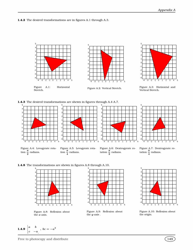
Appendix A
1.4.2 The desired transformations are in figures A.1 through A.3.
-4 -3 -2 -1 0 1 2 3 4 5-4
-3
-2
-1
0
1
2
3
4
5
Figure A.1: HorizontalStretch.
-4 -3 -2 -1 0 1 2 3 4 5-4
-3
-2
-1
0
1
2
3
4
5
Figure A.2: Vertical Stretch.
-4 -3 -2 -1 0 1 2 3 4 5-4
-3
-2
-1
0
1
2
3
4
5
Figure A.3: Horizontal andVertical Stretch.
1.4.3 The desired transformations are shewn in figures through A.4 A.7.
-4 -3 -2 -1 0 1 2 3 4 5-4
-3
-2
-1
0
1
2
3
4
5
Figure A.4: Levogyrate rota-
tionπ
2radians.
-4 -3 -2 -1 0 1 2 3 4 5-4
-3
-2
-1
0
1
2
3
4
5
Figure A.5: Levogyrate rota-
tionπ
4radians.
-4 -3 -2 -1 0 1 2 3 4 5-4
-3
-2
-1
0
1
2
3
4
5
Figure A.6: Dextrogyrate ro-
tationπ
2radians.
-4 -3 -2 -1 0 1 2 3 4 5-4
-3
-2
-1
0
1
2
3
4
5
Figure A.7: Dextrogyrate ro-
tationπ
4radians.
1.4.8 The transformations are shewn in figures A.8 through A.10.
-4 -3 -2 -1 0 1 2 3 4 5-4
-3
-2
-1
0
1
2
3
4
5
Figure A.8: Reflexion aboutthe x-axis.
-4 -3 -2 -1 0 1 2 3 4 5-4
-3
-2
-1
0
1
2
3
4
5
Figure A.9: Reflexion aboutthe y-axis .
-4 -3 -2 -1 0 1 2 3 4 5-4
-3
-2
-1
0
1
2
3
4
5
Figure A.10: Reflexion aboutthe origin.
1.4.9
a b
c −a
, bc = −a2
Free to photocopy and distribute 149

Answers and Hints
1.5.1 Upon solving the equations
−3a1 + 2a2 = 0, a21 + a2
2 = 13
we find (a1, a2) = (2, 3) or (a1, a2) = (−2,−3).
1.5.2 Since −→a •−→b = 0, we have
||−→a +−→b ||2 = (−→a +
−→b )•(−→a +
−→b )
= −→a •−→a + 2−→a •−→b +
−→b •−→b
= −→a •−→a + 0 +−→b •−→b
= ||−→a ||2 + ||−→b ||2,
from where the desired result follows.
1.5.3 By the CBS Inequality,(a2 · 1 + b2 · 1) ≤ (a4 + b4)1/2(12 + 12)1/2,
whence the assertion follows.
1.5.4 We have ∀−→v ∈ R2,−→v • (−→a − −→b ) = 0. In particular, choosing −→v = −→a − −→b , we gather
(−→a − −→b )•(−→a − −→b ) = ||−→a − −→b ||2 = 0.
But the norm of a vector is 0 if and only if the vector is the−→0 vector. Therefore −→a − −→b =
−→0 , i.e., −→a =
−→b .
1.5.5 We have
||−→u +−→v ||2 − ||−→u − −→v ||2 = (−→u +−→v )•(−→u + −→v )− (−→u − −→v )•(−→u − −→v )
= −→u •−→u + 2−→u •−→v +−→v •−→v − (−→u •−→u − 2−→u •−→v +−→v •−→v )
= 4−→u •−→v ,
giving the result.
1.5.6 A parametric equation for L1 is x
y
=
0
b1
+ t
1
m1
.
A parametric equation for L2 is x
y
=
0
b2
+ t
1
m2
.
The lines are perpendicular if and only if, according to Corollary 22,1
m1
•
1
m2
= 0 ⇐⇒ 1 + m1m2 = 0 ⇐⇒ m1m2 = −1.
1.5.7 The line L has a parametric equation x
y
=
0
1
+ t
1
−1
.
Let L′ have parametric equation x
y
=
0
b
+ t
1
m
.
We need the angle between
1
m
and
1
−1
to be
π
6and so by Theorem 21,
1−m =p
1 + m2√
2 cosπ
6=⇒ m = −2±
√3.
This gives two possible values for the slope of L′. Now, since L′ must pass through
−1
2
y = (−2±
√3)x + b =⇒ 2 = (−2±
√3)(−1) + b =⇒ b = ±
√3
and the lines are y = (−2 +√
3)x +√
3 and y = (−2−√
3)x −√
3, respectively.
Free to photocopy and distribute 150

Appendix A
1.5.8 We must prove that −→a •−→w = 0. Using the distributive law for the dot product,−→v −
−→v •−→w−→w 2−→w • −→w = −→v •−→w −−→v •−→w−→w 2−→w •−→w
= −→v •−→w −−→v •−→w−→w 2 −→w 2
= −→v •−→w − −→v •−→w= 0.
1.6.1 We have y − x = 4t =⇒ t =y − x
4and so
x =
y − x
4
3
− 2
y − x
4
is the Cartesian equation sought.
1.6.2 Observe that for t 6= 0,−1,
y
x= t =⇒ x =
y
x
21 +
y
x
5 =⇒ x =y2x3
x5 + y5=⇒ x5 + y5 = x2y2.
If t = 0, then x = 0, y = 0 and our Cartesian equation agrees. What happens as t → −1?
1.6.3
1. ay − cx = ad − bc, this is a straight line with positive slope.
2. −1 ≤ x ≤ 1, y = 0, this is the line segment on the plane joining (−1, 0) to (1, 0).
3.x2
a2− y2
b2= 1, x > 0. This is one branch of a hyperbola.
4.x2
a2− y2
b2= 1. This is a hyperbola.
1.6.4 We may simply give the trivial parametrisation: x = t, y = log cos t, 0 ≤ t ≤ π
3. Then
(dx)2 + (dy)2 = (1 + tan2 t)(dt)2 = sec2 t(dt)2.
Hence the arc length is Z π/3
0
sec tdt = log(2 +√
3).
1.6.5 Observe that y = 2x + 1, so the trace is part of this line. Since in the interval [0; 4π], −1 ≤ sin t ≤ 1, we
want the portion of the line y = 2x + 1 with −1 ≤ x ≤ 1 (and, thus −1 ≤ y ≤ 3). The curve starts at the middle
point (0, 1) (at t = 0), reaches the high point (1, 3) at t =π
2, reaches its low point (−1, 1) at t =
3π
2, reaches its
high point (1, 3) again at t =5π
2, it goes to its low point (−1, 1) at t =
7π
2, and finishes in the middle point (0, 1)
when t = 4π.
1.6.6 First observe that√
x +√
y = 1 demands x ∈ [0; 1] and [0; 1]. Again, one can give many parametrisations.One is x = t2, y = (1− t)2, t ∈ [0; 1]. This givesÈ
(dx)2 + (dy)2 =È
4t2 + (2 − 2t)2 dt = 2p
2t2 − 2t + 1 dt =2√2
É4t − 1
2
2
+ 1 dt.
To integrate
2√2
Z 1
0
É4t − 1
2
2
+ 1 dt,
we now use the trigonometric substitution
2t − 1
2
= tan θ =⇒ dt =
1
2sec2 θdθ.
Free to photocopy and distribute 151
Answers and Hints
The integral thus becomes√
2
Z π/4
0
sec3 θdθ,
the famous secant cube integral, which is a standard example of integration by parts where you “solve” for the
integral. (You write
Zsec θd tan θ = tan θ sec θ −
Ztan θd sec θ, etc.) I will simply quote it, as I assume most of
you have seen it, and it appears in most Calculus texts:
√2
Z π/4
0
sec3 θdθ =√
2
1
2sec θ tan θ − 1
2log | sec θ + tan θ|
π/4
0
=√
2
1
2·√
2 +1
2log(√
2 + 1)
=1√2
log(√
2 + 1) + 1.
1.6.7 First notice that x = 1 =⇒ t3 + 1 = 1 =⇒ t = 0 and x = 2 =⇒ t3 + 1 = 2 =⇒ t = 1. The area
under the graph is Z t=1
t=0
ydx =
Z t=1
t=0
(1− t2)d(t3 + 1) =
Z t=1
t=0
3t2(1− t2)dt =2
5.
1.6.8 Observe that
dx = 6tdt; dy = 6t2dt =⇒È
(dx)2 + (dy)2 = 6tp
1 + t2 dt,
and so the arc length is Z t=1
t=0
È(dx)2 + (dy)2 =
Z t=1
t=0
6tp
1 + t2 dt = 4√
2− 2.
1.6.9 Observe that
dx = tdt, dy =√
2t + 1dt =⇒È
(dx)2 + (dy)2 =È
t2 + (√
2t + 1)2dt =p
t2 + 2t + 1dt = (t + 1)dt.
Hence, the arc length is Z 1/2
−1/2
(1 + t)dt =
t +
t2
2
1/2
−1/2
= 1.
1.6.10 Observe that the parametrisation traverses the curve once clockwise if t ∈ [0; 2π]. The area is given by
1
2
IΓ
det
x dx
y dy
=
1
2
Ixdy − ydx
=4
2
Z 0
π/2
(sin3 t(− sin t(1 + sin2 t) + 2 sin t cos2 t)
− cos t(1 + sin2 t)(3 sin2 t cos t))dt
= 2
Z 0
π/2
(−3 sin2 t + sin4 t)dt
= 2
Z 0
π/2
−9
8+ cos 2t +
1
8cos 4t
dt
=9π
8.
1.6.11 Using the quotient rule,
dx =3(1 + t3)− 3t2(3t)
(1 + t3)2· dt =
3− 6t3
(1 + t3)2· dt =⇒ ydx =
9t2 − 18t5
(1 + t3)3· dt
and
dy =6t(1 + t3)− 3t2(3t2)
(1 + t3)2· dt =
6t − 3t4
(1 + t3)2· dt =⇒ xdy =
18t2 − 9t5
(1 + t3)3· dt
Hence
xdy − ydx =18t2 − 9t5
(1 + t3)3· dt − 9t2 − 18t5
(1 + t3)3· dt =
9t2 + 9t5
(1 + t3)3· dt =
9t2(1 + t3)
(1 + t3)3· dt =
9t2
(1 + t3)2· dt.
Observe that when t = 0 then x = y = 0. As t → +∞, then x → 0 and y → 0. Hence to obtain the loop Using
integration by substitution (u = 1 + t3 and du = 3t2dt) , the area is given by
1
2
Z +∞
0
9t2
(1 + t3)2· dt =
3
2
Z +∞
0
3t2
(1 + t3)2dt =
3
2
Z +∞
1
du
u2=
3
2.
Free to photocopy and distribute 152
Appendix A
A shorter way of obtaining xdy − ydx would have been to argue that xdy − ydx = x2dy
x
=
9t2
(1 + t3)2dt.
1.6.12 See figure 1.58. Let θ be the angle (in radians) of rotation of the circle, and let C be the centre of thecircle. At θ = 0 the centre of the circle is at (0, ρ), and P = (0, ρ − d). Suppose the circle is displaced towardsthe right, making the point P to rotate an angle of θ radians. Then the centre of the circle has displaced rθunits horizontally, and so is now located at (ρθ, ρ). The polar coordinates of the point P are (d sin θ; d cos θ), inrelation to the centre of the circle (notice that the circle moves clockwise). The point P has moved x = ρθ− d sin θhorizontal units and y = ρ − d cos θ units. This is the desired parametrisation.
1.6.14 We have
dx = et(cos t−sin t)dt, dy = et(sin t+cos t)dt =⇒È
(dx)2 + (dy)2 = etÈ
(cos t − sin t)2 + (sin t + cos t)2dt =√
2etdt.
The arc length is thus Z π
0
È(dx)2 + (dy)2 =
√2
Z π
0
etdt =√
2(eπ − 1).
1.6.15 Choose coordinates so that the origin is at the position of the gun, the y-axis is vertical, and the airplaneis on a point with coordinates (u, h) with u ≥ 0.
If the gun were fired at t = 0, then
x = V t cos a; y = V t sin a − gt2
2,
where a is the angle of elevation, t is the time and g is the acceleration due to gravity. Since we know that the
shell strikes the plane, we must have
u = V t cos a; h = V t sin a − gt2
2,
whence
u2 +h +
1
2gt22
= V 2t2,
and thusg2t4
4+ (gh − V 2)2t2 + h2 + u2 = 0.
The quadratic equation in t2 has a real root if
(gh − V 2)2 ≥ g2(h2 + u2) =⇒ g2u2 ≤ V 2(V 2 − 2gh),
from where the assertion follows.
1.6.16 Suppose the parabolas have a point of contact P = (4px20, 4px0). By symmetry, the vertex V of the rolling
parabola is the reflexion of the origin about the line tangent to their point of contact. The slope of the tangent at P
is1
2x0, from where the equation of the tangent is
y =x
2x0+ 2px0.
The line normal to this line and passing through the origin is hence
y = −2xx0,
and so the lines intersect at − 4px2
0
1 + 4x20
,8px3
0
1 + 4x20
,
from where
V =
− 8px2
0
1 + 4x20
,16px3
0
1 + 4x20
:= (x(t), y(t)).
As −2x0x(t) = y(t), eliminating t yields
x = − 2p
yx
21 +
yx
2or
(x2 + y2)x + 2py2 = 0,
giving the equation of the locus.
Free to photocopy and distribute 153
Answers and Hints
1.7.1 Observe that, in general,−→a − −→b 2 +−→a +
−→b2 =
−→a 2 − 2−→a •−→b +
−→b 2 +−→a 2 + 2−→a •
−→b +
−→b 2= 2
−→a 2 + 2−→b 2,
whence −→a − −→b = É2−→a 2 + 2
−→b 2 − −→a +−→b = È
2(13)2 + 2(19)2 − (24)2 = 22.
1.7.2
x
y
z
DZ=
1
2
3
DZ+ t
264−2
−1
0
375 .
1.7.3 The vectorial form of the equation of the line is
−→r =
2641
0
1
375+ t
264 1
−2
−1
375 .
Since the line follows the direction of
264 1
−2
−1
375, this means that
264 1
−2
−1
375 is normal to the plane, and thus the equation
of the desired plane is(x − 1)− 2(y − 1) − (z − 1) = 0.
1.7.4 Observe that
0
0
0
DZ(as 0 = 2(0) = 3(0)) is on the line, and hence on the plane. Thus the vector264 1− 0
−1− 0
−1− 0
375 =
264 1
−1
−1
375lies on the plane. Now, if x = 2y = 3z = t, then x = t, y = t/2, z = t/3. Hence, the vectorial form of the equationof the line is
−→r =
2640
0
0
375+ t
264 1
1/2
1/3
375 = t
264 1
1/2
1/3
375 .
This means that
264 1
1/2
1/3
375 also lies on the plane, and thus264 1
−1
−1
375× 264 1
1/2
1/3
375 =
264 1/6
−4/3
3/2
375is normal to the plane. The desired equation is thus
1
6x − 4
3y +
3
2z = 0.
1.7.5 The set B can be decomposed into the following subsets:
➊ The set A itself, of volume abc.
➋ Two a × b × 1 bricks, two b × c × 1 bricks, and two c × a × 1 bricks,
➌ Four quarter-cylinders of length a and radius 1, four quarter-cylinders of length b and radius 1, and four
quarter-cylinders of length c and radius 1,
Free to photocopy and distribute 154
Appendix A
➍ Eight eighth-of-spheres of radius 1.
Thus the required formula for the volume is
abc + 2(ab + bc + ca) + π(a + b + c) +4π
3.
1.7.6 We have,−→a +−→b +−→c
2 = (−→a +−→b + −→c ) • (−→a +
−→b +−→c ) =
−→a 2 +−→b 2 +
−→c 2 + 2(−→a •−→b +
−→b •−→c + −→c •−→a ),
from where we deduce that−→a •−→b +
−→b •−→c +−→c •−→a =
−32 − 42 − 52
2= −25.
1.7.7 A vector normal to the plane is
264 a
a2
a2
375. The line sought has the same direction as this vector, thus the
equation of the line is 264x
y
z
375 =
2640
0
1
375+ t
264 a
a2
a2
375 , t ∈ R.
1.7.8 Put ax = by = cz = t, so x = t/a; y = t/b; z = t/c. The parametric equation of the line is264x
y
z
375 = t
2641/a
1/b
1/c
375 , t ∈ R.
Thus the vector
2641/a
1/b
1/c
375 is perpendicular to the plane. Therefore, the equation of the plane is2641/a
1/b
1/c
375 •
264x − 1
y − 1
z − 1
375 =
2640
0
0
375 ,
orx
a+
y
b+
z
c=
1
a+
1
b+
1
c.
We may also write this asbcx + cay + abz = ab + bc + ca.
1.7.9 The vector
264 1
−1
1
375 is perpendicular to the plane. Hence, the shortest distance from (1, 2, 3) is obtained by
the perpendicular line to the plane that pierces the plane, this perpendicular line to the plane has equationx
y
z
DZ=
1
2
3
DZ+ t
264 1
−1
1
375 =⇒ x = 1 + t, y = 2− t, z = 3 + t.
The intersection of the line and the plane occurs when
1 + t − (2− t) + (3 + t) = 1 =⇒ t = −1
3.
The closest point on the plane to (1, 2, 3) is therefore
2
3,7
3,8
3
, and the distance sought isÉ
(1− 2
3)2 + (2 − 7
3)2 + (3 − 8
3)2 =
√3
3.
Free to photocopy and distribute 155
Answers and Hints
1.7.10 If the lines intersected, there would be a value t′ for which1
1
1
DZ+ t′
2642
1
1
375 =
0
0
1
DZ+ t′
264 2
−1
1
375 =⇒
2641− 0
1− 0
1− 1
375 = t′
264 2− 2
−1− 1
1− 1
375 =⇒
2641
1
0
375 = t′
264 0
−2
0
375 ,
which is clearly impossible, and so the lines are skew. Let θ be the angle between them. Then
cos θ =2 · 2 + 1 · (−1) + 1 · 1p
(2)2 + (1)2 + (1)2p
(2)2 + (−1)2 + (1)2=
4√6√
6=⇒ θ = arccos
2
3
.
1.7.11 Observe the CBS Inequality in R3 given the vectors −→x = (x1, x2, x3),
−→y = (y1, y2, y3) let θ be the angle
between them. Then
−→x •−→y =−→x −→y cos θ =⇒ |x1y1 + x2y2 + x3y3| ≤
Èx2
1 + x22 + x2
3
Èy21 + y2
2 + y23 .
Now take x1 = a2, x2 = b2, x3 = c2 and y1 = y2 = y3 = 1. This gives (since squares are positive, we don’t needthe absolute values)
|x1y1 + x2y2 + x3y3| ≤È
x21 + x2
2 + x23
Èy21 + y2
2 + y23 =⇒ (a2 + b2 + c2)2 ≤ (a4 + b4 + c4)(3),
which proves the claim at once.
1.7.12 First observe that
S(a, b, c) =È
s(s − a)(s − b)(s − c)
=1
4
È(a + b + c)(b + c − a)(c + a − b)(a + b − c)
=1
4
È(a2 + b2 + c2)2 − 2(a4 + b4 + c4)
Hence
S(a, b, c)
a2 + b2 + c2=
1
4
r1− 2
a4 + b4 + c4
(a2 + b2 + c2)2,
and thus maximising f is equivalent to minimising 2a4 + b4 + c4
(a2 + b2 + c2)2. From problem 1.7.11,
a4 + b4 + c4
(a2 + b2 + c2)2≥ 1
3,
which in turn gives
S(a, b, c)
a2 + b2 + c2≤ 1
4
É1− 2
3=
1
4√
3=
√3
12,
the desired maximum.
1.7.15 x + y + z = 1.1
6.
1.7.16 Assume contrariwise that −→a ,−→b , −→c are three unit vectors in R
3 such that the angle between any two of
them is >2π
3. Then −→a •
−→b < −1
2,−→b •−→c < −1
2, and −→c •−→a < −1
2. Thus−→a +
−→b +−→c
2 =−→a 2 +
−→b 2 +−→c 2
+2−→a •−→b + 2
−→b •−→c + 2−→c •−→a
< 1 + 1 + 1− 1− 1− 1
= 0,
which is impossible, since a norm of vectors is always ≥ 0.
Free to photocopy and distribute 156

Appendix A
1.7.17 Let projts =
−→t •−→s
(||s||)2−→s be the projection of
−→t over −→s 6= −→0 . Let x0 be the point on the plane that is nearest
to b. Then−→bx0 = −→x0 −
−→b is orthogonal to the plane, and the distance we seek is
||proj−→r0−−→
bn || =
(−→r0 − −→b )•−→n−→n 2 −→n = |(−→r0 − −→b )•−→n |−→n .
Since R0 is on the plane, −→r0 •−→n = −→a •−→n , and so
||proj−→r0−−→
bn || = |
−→r0 •−→n − −→b •−→n |−→n | =|−→a •−→n − −→b •−→n |−→n =
|(−→a − −→b )•−→n |−→n ,
as we wanted to shew.
1.7.18 There are 7 vertices (V0 = (0, 0, 0), V1 = (11, 0, 0), V2 = (0, 9, 0), V3 = (0, 0, 8), V4 = (0, 3, 8), V5 =(9, 0, 2), V6 = (4, 7, 0)) and 11 edges (V0V1, V0V2, V0V3, V1V5, V1V6, V2V4, V2V6, V3V4, V3V5, V4V5, and V4V6).
x y
z
Figure A.11: Problem 1.7.18.
1.8.2 We have −→x × −→x = −−→x × −→x by letting −→y = −→x in ??. Thus 2−→x × −→x =−→0 and hence −→x × −→x =
−→0 .
1.8.3 One has
(−→b − −→a )× (−→c − −→a ) =
−→0 =⇒ −→a × −→b +
−→b × −→c + −→c × −→a =
−→0
This gives−→b × −→c = −(−→a × −→b +−→c × −→a ) = −(
−→j +−→k +
−→i − −→j ) = −−→i − −→k .
1.8.4 The vector
2641
1
1
375× 2641
1
0
375 =
264−1
1
0
375 is normal to the plane. The plane has thus equation264 x
y + 1
z − 2
375 •
264−1
1
0
375 = 0 =⇒ −x + y + 1 = 0 =⇒ x − y = 1,
as obtained before.
1.8.5 The vectors 264a − (−a)
0− 1
a − 0
375 =
2642a
−1
a
375and 2640− (−a)
1− 1
2a − 0
375 =
264 a
0
2a
375Free to photocopy and distribute 157
Answers and Hints
lie on the plane. A vector normal to the plane is2642a
−1
a
375× 264 a
0
2a
375 =
264−2a
−3a2
a
375 .
The equation of the plane is thus given by 264−2a
−3a2
a
375 •
264x − a
y − 0
z − a
375 = 0,
that is,
2ax + 3a2y − az = a2.
1.8.6 Either of−→v × −→w||−→v × −→w || or −
−→v × −→w||−→v × −→w || will do. Now
−→v × −→w = (−a−→j + a
−→k )× (
−→i + a
−→j )
= −a(−→j × −→i )− a2(
−→j × −→j ) + a(
−→k × −→i ) + a2(
−→k × −→j )
= a−→k + a
−→j − a2−→i
=
−a2
a
a
DZ,
and ||−→v × −→w || =p
a4 + a2 + a2 =p
2a2 + a4. Hence we may take either
1√2a2 + a4
−a2
a
a
DZor
− 1√2a2 + a4
−a2
a
a
DZ.
1.8.7 From Theorem ?? we have
−→a × (−→b × −→c ) = (−→a •−→c )
−→b − (−→a •
−→b )−→c ,
−→b × (−→c × −→a ) = (
−→b •−→a )−→c − (
−→b •−→c )−→a ,
−→c × (−→a × −→b ) = (−→c •−→b )−→a − (−→c •−→a )
−→b ,
and adding yields the result.
1.8.8 By Lagrange’s Identity,
||−→x × −→i ||2 =−→x 2−→i 2 − (−→x •
−→i )2 = 1− (−→x •
−→i )2,
||−→x × −→k ||2 =−→x 2−→j 2 − (−→x •
−→j )2 = 1− (−→x •
−→j )2,
||−→x × −→j ||2 =−→x 2−→k 2 − (−→x •
−→k )2 = 1− (−→x •
−→k )2,
and since (−→x •−→i )2 + (−→x •
−→j )2 + (−→x •
−→k )2 =
−→x 2 = 1, the desired sum equals 3− 1 = 2.
1.8.9
−→a × (−→x ×−→b ) =−→b × (−→x ×−→a ) ⇐⇒ (−→a •
−→b )−→x − (−→a •−→x )
−→b = (
−→b •−→a )−→x − (
−→b •−→x )−→a ⇐⇒ −→a •−→x =
−→b •−→x = 0.
The answer is thus −→x : −→x ∈ R−→a × −→b .
Free to photocopy and distribute 158
Appendix A
1.8.12
−→x =(−→a •−→b )−→a + 6
−→b + 2−→a × −→c
12 + 2−→a 2
−→y =(−→a •−→c )−→a + 6−→c + 3−→a × −→b
18 + 3−→a 2
1.8.13 First observe that−→x • (−→y × −→z ) = (−→x × −→y ) • −→z .
This is so because both sides give the volume of the parallelogram spanned by −→x , −→y , −→z . Now, putting −→x =−→a × −→b , −→y = −→c and −→z =
−→d we gather that
(−→a × −→b ) • (−→c × −→d ) = ((−→a × −→b )× −→c ) • −→d .
Now, again,
(−→a × −→b )× −→c = −−→c × (−→a × −→b ) = −((−→c •−→b )−→a − (−→c •−→a )
−→b ) = (−→c •−→a )
−→b − (−→c •
−→b )−→a .
This gives
((−→a × −→b )× −→c ) • −→d = ((−→c •−→a )−→b − (−→c •
−→b )−→a ) • −→d = (−→c •−→a )(
−→b •−→d )− (−→c •
−→b )(−→a •
−→d ),
proving the identity.
1.8.14 By problem 1.8.13,
(−→x × −→y ) • (−→u × −→v ) = (−→x •−→u ) • (−→y •−→v )− (−→x •−→v ) • (−→y •−→u ).
Using this three times:
(−→b × −→c ) • (−→a × −→d ) = (
−→b •−→a ) • (−→c •
−→d )− (
−→b •−→d ) • (−→c •
−→d )
(−→c × −→a ) • (−→b × −→d ) = (−→c •
−→b ) • (−→a •
−→d )− (−→c •
−→d ) • (−→a •
−→b )
(−→a × −→b ) • (−→c × −→d ) = (−→a •−→c ) • (−→b •−→d )− (−→a •
−→d ) • (
−→b •−→c )
Adding these three equalities, and using the fact that the dot product is commutative, we see that all the terms onthe dextral side cancel out and we obtain 0, as required.
1.8.15
1. We have
−→CA =
264 6
0
−3
375 ,−→CB =
264 0
4
−3
375 =⇒ −→CA×−→CB = (6
−→i − 3
−→k )× (4
−→j − 3
−→k ) = 24
−→k +18
−→j + 12
−→i =
26412
18
24
375 .
2. We have −→CA × −→CB
= p122 + 182 + 242 =
√1044 = 6
√29.
3. The desired line has equationx
y
z
DZ=
0
0
3
DZ+ t
264 6
0
−3
375 =⇒ x = 6t, y = 0, z = 3− 3t.
4. The desired line has equationx
y
z
DZ=
3
0
0
DZ+ s
264 0
0
−3
375 =⇒ x = 3, y = 0, z = −3s.
Free to photocopy and distribute 159
Answers and Hints
5. From the preceding items, the line LCA is x = 6t, y = 0, z = 3 − 3t and the line LDE is x = 3, y =
0, z = −3s. If the line intersect then 6t = 3, 0 = 0, 3 − 3t = −3s gives t =1
2and s = −1
2. The point of
intersection is thus3, 0,
3
2
. item The area is
1
2
−→CA× −→CB = 1
2· 6√
29 = 3√
29.
6. Observe that
P =
3
0
z
DZ, Q =
3
y
0
DZ, R =
x
3
0
DZ, S =
0
3
z
DZ.
Since all this points lie on the plane 2x + 3y + 4z = 12, we find
2(3) + 3(0) + 4z = 12 =⇒ P =
3
03
2
DZ,
2(3) + 3y + 4(0) = 12 =⇒ Q =
3
2
0
DZ,
2x + 3(3) + 4(0) = 12 =⇒ R =
3
23
0
DZ,
2(0) + 3(3) + 4z = 12 =⇒ S =
0
33
4
DZ.
7. A possible way is to decompose the pentagon into three triangles, say 4CP Q, 4CQR and 4CRS and findtheir areas. Another way would be to subtract from the area of 4ABC the areas of 4AP Q and 4RSB. I
will follow the second approach. Let [4AP Q], [4RSB] denote the areas of4AP Q and4RSB respectively.Then
[4AP Q] =1
2
−→PA× −→PQ
= 1
2
2643
03
2
375× 264 0
2
−3
2
375 = 1
2
264−39
26
375 = 1
2
É9 +
81
4+ 36 =
3
4
√29,
[4RSB] =1
2
−→SR× −→SB = 1
2
2664 3
20
−3
4
3775× 264 0
1
−3
4
375 = 1
2
26643
49
83
2
3775 = 1
2
É9
16+
81
64+
9
4=
3
16
√29.
Hence the area of the pentagon is
3√
29− 3
4
√29− 3
16
√29 =
33
16
√29.
1.9.2 The assertion is trivial for n = 1. Assume its truth for n − 1, that is, assume An−1 = 3n−2A. Observe that
A2 =
2641 1 1
1 1 1
1 1 1
3752641 1 1
1 1 1
1 1 1
375 =
2643 3 3
3 3 3
3 3 3
375 = 3A.
NowAn = AAn−1 = A(3n−2A) = 3n−2A2 = 3n−23A = 3n−1A,
and so the assertion is proved by induction.
Free to photocopy and distribute 160
Appendix A
1.9.3 First, we will prove that
A2 =
26666664 1 2 3 4 . . . n − 1 n
0 1 2 3 . . . n − 2 n − 1
0 0 1 2 . . . n − 3 n − 2
. . . . . ....
...... . . . . . .
0 0 0 0 . . . 0 1
37777775 .
Observe that A = [aij ], where aij = 1 for i ≤ j and aij = 0 for i > j.
Put A2 = [bij ]. Assume first that i ≤ j. Then
bij =
nXk=1
aikakj =
jXk=i
1 = j − i + 1.
Assume now that i > j. Then
bij =
nXk=1
aikakj =
nXk=1
0 = 0,
proving the first statement. Now, we will prove that
A3 =
26666666664 1 3 6 10 . . .(n − 1)n
2
n(n + 1)
2
0 1 3 6 . . .(n − 2)(n − 1)
2
(n − 1)n
2
0 0 1 3 . . .(n − 3)(n − 2)
2
(n − 2)(n − 1)
2
. . . . . ....
...... . . . . . .
0 0 0 0 . . . 0 1
37777777775 .
For the second part, you need to know how to sum arithmetic progressions. In our case, we need to know how tosum (assume i ≤ j),
S1 =
jXk=i
a, S2 =
jXk=i
k.
The first sum is trivial: there are j − i + 1 integers in the interval [i; j], and hence
S1 =
jXk=i
a = S1 = a
jXk=i
1 = a(j − i + 1).
For the second sum, we use Gauß trick: summing the sum forwards is the same as summing the sum backwards,and so, adding the first two rows below,
S2 = i + i + 1 + i + 2 + · · · + j − 1 + j
S2 = j + j − 1 + j − 2 + · · · + i− 1 + i
2S2 = (i + j) + (i + j) + (i + j) + · · · + (i + j) + (i + j)
2S2 = (i + j)(j − i + 1) · · ·
,
which gives S2 =(i + j)(j − i + 1)
2.
Put now A3 = [cij ]. Assume first that i ≤ j. Since A3 = A2A,
cij =
nXk=1
bikakj
=
jXk=i
(k − i + 1)
=
jXk=i
k −jX
k=i
i +
jXk=i
1
=(j + i)(j − i + 1)
2− i(j − i + 1) + (j − i + 1)
=(j − i + 1)(j − i + 2)
2.
Free to photocopy and distribute 161
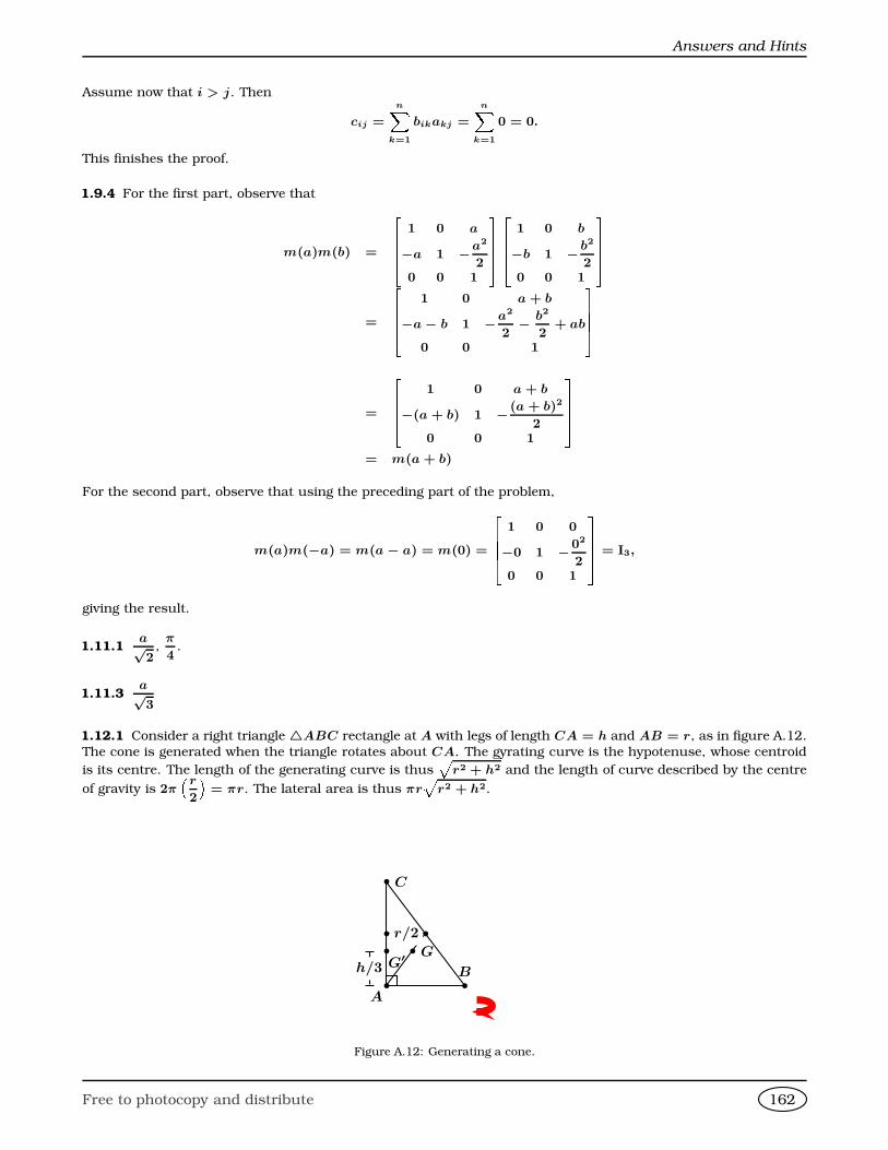
Answers and Hints
Assume now that i > j. Then
cij =
nXk=1
bikakj =
nXk=1
0 = 0.
This finishes the proof.
1.9.4 For the first part, observe that
m(a)m(b) =
2664 1 0 a
−a 1 −a2
20 0 1
37752664 1 0 b
−b 1 − b2
20 0 1
3775=
2664 1 0 a + b
−a − b 1 −a2
2− b2
2+ ab
0 0 1
3775=
2664 1 0 a + b
−(a + b) 1 − (a + b)2
20 0 1
3775= m(a + b)
For the second part, observe that using the preceding part of the problem,
m(a)m(−a) = m(a − a) = m(0) =
2664 1 0 0
−0 1 −02
20 0 1
3775 = I3,
giving the result.
1.11.1a√2
,π
4.
1.11.3a√3
1.12.1 Consider a right triangle 4ABC rectangle at A with legs of length CA = h and AB = r, as in figure A.12.
The cone is generated when the triangle rotates about CA. The gyrating curve is the hypotenuse, whose centroid
is its centre. The length of the generating curve is thusp
r2 + h2 and the length of curve described by the centre
of gravity is 2πr
2
= πr. The lateral area is thus πr
pr2 + h2.
b
Ab
B
b C
b b
b Gb
G′h/3
r/2
Figure A.12: Generating a cone.
Free to photocopy and distribute 162
Appendix A
To find the volume, we gyrate the whole right triangle, whose area isrh
2. We need to find the centroid of the
triangle. But from example 17, we know that the centroid G of the triangle is is two thirds of the way from A to
the midpoint of BC. If G′ is the perpendicular projection of G onto [CA], then this means that G′ is at a vertical
height ofh
2· 23
=h
3. By similar triangles
GG′
r=
h/3
h=⇒ GG′ =
r
3. Hence, the length of the curve described
by the centre of gravity of the triangle is2
3πr. The volume of the cone is thus
2
3πr · rh
2=
π
3r2h.
1.14.1 Find a vector −→a mutually perpendicular to−−−→V1V2 and
−−−→V1V3 and another vector and a vector
−→b mutually
perpendicular to−−−→V1V3 and
−−−→V1V4. Then shew that cos θ =
1
3, where θ is the angle between −→a and
−→b .
1.15.1 Let
x
y
z
DZbe a point on S. If this point were on the xz plane, it would be on the ellipse, and its distance
to the axis of rotation would be |x| =1
2
p1− z2. Anywhere else, the distance from
x
y
z
DZto the z-axis is the
distance of this point to the point
0
0
z
DZ:p
x2 + y2. This distance is the same as the length of the segment on
the xz-plane going from the z-axis. We thus havepx2 + y2 =
1
2
p1− z2,
or
4x2 + 4y2 + z2 = 1.
1.15.2 Let
x
y
z
DZbe a point on S. If this point were on the xy plane, it would be on the line, and its distance to
the axis of rotation would be |x| = 1
3|1 − 4y|. Anywhere else, the distance of
x
y
z
DZto the axis of rotation is the
same as the distance of
x
y
z
DZto
0
y
0
DZ, that is
px2 + z2. We must havep
x2 + z2 =1
3|1− 4y|,
which is to say
9x2 + 9z2 − 16y2 + 8y − 1 = 0.
1.15.3 A spiral staircase.
1.15.4 A spiral staircase.
1.15.6 The planes A : x + z = 0 and B : y = 0 are secant. The surface has equation of the form f(A, B) =
eA2+B2 − A = 0, and it is thus a cylinder. The directrix has direction−→i − −→k .
1.15.7 Rearranging,
(x2 + y2 + z2)2 − 1
2((x + y + z)2 − (x2 + y2 + z2)) − 1 = 0,
and so we may take A : x + y + z = 0, Σ : x2 + y2 + z2 = 0, shewing that the surface is of revolution. Its axis is
the line in the direction−→i +−→j +−→k .
Free to photocopy and distribute 163
Answers and Hints
1.15.8 Considering the planes A : x − y = 0, B : y − z = 0, the equation takes the form
f(A, B) =1
A+
1
B− 1
A + B− 1 = 0,
thus the equation represents a cylinder. To find its directrix, we find the intersection of the planes x = y and
y = z. This gives
264x
y
z
375 = t
2641
1
1
375. The direction vector is thus−→i +−→j +−→k .
1.15.9 Rearranging,
(x + y + z)2 − (x2 + y2 + z2) + 2(x + y + z) + 2 = 0,
so we may take A : x + y + z = 0, Σ : x2 + y2 + z2 = 0 as our plane and sphere. The axis of revolution is then in
the direction of−→i +−→j +−→k .
1.15.10 After rearranging, we obtain
(z − 1)2 − xy = 0,
or
− x
z − 1
y
z − 1+ 1 = 0.
Considering the planes
A : x = 0, B : y = 0, C : z = 1,
we see that our surface is a cone, with apex at (0, 0, 1).
1.15.11 The largest circle has radius b. Parallel cross sections of the ellipsoid are similar ellipses, hence we mayincrease the size of these by moving towards the centre of the ellipse. Every plane through the origin which makes a
circular cross section must intersect the yz-plane, and the diameter of any such cross section must be a diameter
of the ellipse x = 0,y2
b2+
z2
c2= 1. Therefore, the radius of the circle is at most b. Arguing similarly on the xy-plane
shews that the radius of the circle is at least b. To shew that circular cross section of radius b actually exist, onemay verify that the two planes given by a2(b2 − c2)z2 = c2(a2 − b2)x2 give circular cross sections of radius b.
1.15.12 Any hyperboloid oriented like the one on the figure has an equation of the form
z2
c2=
x2
a2+
y2
b2− 1.
When z = 0 we must have
4x2 + y2 = 1 =⇒ a =1
2, b = 1.
Thusz2
c2= 4x2 + y2 − 1.
Hence, letting z = ±2,
4
c2= 4x2 + y2 − 1 =⇒ 1
c2= x2 +
y2
4− 1
4= 1− 1
4=
3
4,
since at z = ±2, x2 +y2
4= 1. The equation is thus
3z2
4= 4x2 + y2 − 1.
1.16.1 The arc length element isÈ(dx)2 + (dy)2 + (dz)2 =
p4t2 + 36t + 81 dt = (2t + 9) dt.
We need t = 1 to t = 4. The desired length isZ 4
1
(2t + 9) dt = (t2 + 9t)41
= (16 + 36)− (1 + 9) = 42.
Free to photocopy and distribute 164
Appendix A
1.16.2 Observe that z = 1+x2+y2 is a paraboloid opening up, with vertex (lowest point) at (0, 0, 1). On the other
hand, z = 3 − x2 − y2 is another paraboloid opening down, with highest point at (0, 0, 3). Adding the equationswe obtain
2z = z + z = (1 + x2 + y2) + (3− x2 − y2) = 4 =⇒ 2z = 4 =⇒ z = 2,
so they intersect at the plane z = 2. Subtracting the equations,
(1 + x2 + y2)− (3 − x2 − y2) = z − z = 0 =⇒ 2x2 + 2y2 − 2 = 0 =⇒ x2 + y2 = 1,
so they intersect at the circle x2 + y2 = 1, z = 2. Since they meet at the circle x2 + y2 = 1, we may parametrisethis circle as x = cos t, y = sin t, t ∈ [0; 2π], z = 2.
1.16.3 Let −→r (t) lie on the plane ax + by + cz = d. Then we must have
at4
1 + t2+ b
t3
1 + t2+ c
t2
1 + t2= d =⇒ (at4 + bt3 + ct2) = d(1 + t2) =⇒ at4 + bt3 + (c − d)t2 − d = 0,
which means that if −→r (t) is on the plane ax + by + cz = d, then t must satisfy the quartic polynomial p(t) =at4 + bt3 + (c− d)t2 − d = 0. Hence, the tk are coplanar if and only if they are roots of p(t). Since the coefficient
of t in this polynomial is 0, then the sum of the roots of p(t) taken three at a time is 0, that is,
t1t2t3 + t1t2t4 + t1t3t4 + t2t3t4 = 0 =⇒ t1t2t3 + t1t2t4 + t1t3t4 + t2t3t4t1t2t3t4
= 0 =⇒ 1
t1+
1
t2+
1
t3+
1
t4= 0,
as required.
1.16.4 Observe that in this problem you are only parametrising the ellipsoid! The tricky part is to figure out
the bounds in your parameters so that only the part above the plane x + y + z = 0 is described. A commonparametrisation found was:
x = cos θ sin φ, y = 3 sin θ sin φ, z = cos φ.
The projection of the plane x + y + z = 0 onto the xy-plane is the line y = −x. To be “above” this line, the angle
θ, measured from the positive x-axis needs to be in the interval −π
4≤ θ ≤ 3π
4. Since
2641
1
1
375 is normal to the plane
x + y + z = 0, the plane makes an angle ofπ
4with the z-axis. Recall that φ is measured from φ = 0 (positive
z-axis) to φ = π (negative z-axis). Hence to be above the plane we need 0 ≤ φ ≤ 3π
4.
1.16.6
1.
264 −2a
a2 − 1
a2 + 1
3752. x2 + y2 = c2 + 1
3. π
Z 1
0
(c2 + 1)dc =4π
3
1.17.1
1. Put f : R→ R, f(x) = ex−1 − x. Clearly f(1) = e0 − 1 = 0. Now,
f ′(x) = ex−1 − 1,
f ′′(x) = ex−1.
If f ′(x) = 0 then ex−1 = 1 implying that x = 1. Thus f has a single minimum point at x = 1. Thus for allreal numbers x
0 = f(1) ≤ f(x) = ex−1 − x,
which gives the desired result.
2. Easy Algebra!
3. Easy Algebra!
Free to photocopy and distribute 165
Answers and Hints
4. By the preceding results, we have
A1 ≤ exp(A1 − 1),
A2 ≤ exp(A2 − 1),
...
An ≤ exp(An − 1).
Since all the quantities involved are non-negative, we may multiply all these inequalities together, to obtain,
A1A2 · · ·An ≤ exp(A1 + A2 + · · ·+ An − n).
In view of the observations above, the preceding inequality is equivalent to
nnGn
(a1 + a2 + · · ·+ an)n≤ exp(n − n) = e0 = 1.
We deduce that
Gn ≤
a1 + a2 + · · ·+ an
n
n
,
which is equivalent to
(a1a2 · · · an)1/n ≤ a1 + a2 + · · ·+ an
n.
Now, for equality to occur, we need each of the inequalities Ak ≤ exp(Ak−1) to hold. This occurs, in view of
the preceding lemma, if and only if Ak = 1, ∀k, which translates into a1 = a2 = . . . = an . This completesthe proof.
1.17.2 By CBS,
(x1 + x2 + . . . + xn)
1
x1+
1
x2+ . . . +
1
xn
≥
nX
i=1
√xi
1√xi
2
= n2.
1.17.3 By CBS,
(a + b + c + d)2 ≤ (1 + 1 + 1 + 1)a2 + b2 + c2 + d2 = 4
a2 + b2 + c2 + d2 .
Hence,
(8− e)2 ≤ 416− e2 ⇐⇒ e (5e − 16) ≤ 0 ⇐⇒ 0 ≤ e ≤ 16
5.
The maximum value e =16
5is reached when a = b = c = d =
6
5.
1.17.4 Observe that 96 · 216 = 1442 and by CBS,
nXk=1
a2k ≤
nX
k=1
a3k
nX
k=1
ak
.
As there is equality,(a1, a2, . . . , an) = t(a3
1, a32, . . . , a3
n)
for some real number t. Hence a1 = a2 = . . . = an = a, from where na = 96, na2 = 144 gives a =3
2y n = 32.
1.17.5 Applying the AM-GM inequality, for 1, 2, . . . , n:
n!1/n = (1 · 2 · · · n)1/n <1 + 2 + · · ·+ n
n=
n + 1
2,
with strict inequality for n > 1.
1.17.6 If x ∈ [−a; a], then a + x ≥ 0 and a − x ≥ 0, and thus we may use AM-GM with n = 8, a1 = a2 = · · · =a5 =
a + x
5and a6 = a7 = a8 =
a − x
3. We deduce that
a + x
5
5 a − x
3
3
≤
5
a + x
5
+ 3
a − x
3
8
8
=a
4
8,
from where
f(x) ≤ 5533a8
48,
with equality if and only ifa + x
5=
a − x
3.
Free to photocopy and distribute 166
Appendix A
1.17.7 Applying AM-GM to the set of n + 1 numbers
1, 1 +1
n, 1 +
1
n, . . . , 1 +
1
n,
has arithmetic mean
1 +1
n + 1
and geometric mean 1 +
1
n
n/(n+1)
.
Therefore,
1 +1
n + 1>1 +
1
n
n/(n+1)
,
that is 1 +
1
n + 1
n+1
>1 +
1
n
n
,
which means
xn+1 > xn,
giving the assertion.
2.1.2 Since polynomials are continuous functions and the image of a connected set is connected for a continuousfunction, the image must be an interval of some sort. If the image were a finite interval, then f(x, kx) would be
bounded for every constant k, and so the image would just be the point f(0, 0). The possibilities are thus
1. a single point (take for example, p(x, y) = 0),
2. a semi-infinite interval with an endpoint (take for example p(x, y) = x2 whose image is [0;+∞[),
3. a semi-infinite interval with no endpoint (take for example p(x, y) = (xy− 1)2 +x2 whose image is ]0;+∞[),
4. all real numbers (take for example p(x, y) = x).
2.3.4 0
2.3.5 2
2.3.6 c = 0.
2.3.7 0
2.3.10 By AM-GM,
x2y2z2
x2 + y2 + z2≤ (x2 + y2 + z2)3
27(x2 + y2 + z2)=
(x2 + y2 + z2)2
27→ 0
as (x, y, z)→ (0, 0, 0).
2.4.1 We have
F (−→x +−→h )− F (−→x ) = (−→x +
−→h )× L(−→x +
−→h )− −→x × L(−→x )
= (−→x +−→h )× (L(−→x ) + L(
−→h ))− −→x × L(−→x )
= −→x × L(−→h ) +
−→h × L(−→x ) +
−→h × L(
−→h )
Now, we will prove that ||−→h × L(−→h )|| = o
−→h as−→h → −→0 . For let
−→h =
nXk=1
hk−→e k,
where the −→e k are the standard basis for Rn. Then
L(−→h ) =
nXk=1
hkL(−→e k),
Free to photocopy and distribute 167
Answers and Hints
and hence by the triangle inequality, and by the Cauchy-Bunyakovsky-Schwarz inequality,
||L(−→h )|| ≤
nXk=1
|hk|||L(−→e k)||
≤
nXk=1
|hk|21/2 nX
k=1
||L(−→e k)||21/2
=−→h ( nX
k=1
||L(−→e k)||2)1/2,
whence, again by the Cauchy-Bunyakovsky-Schwarz Inequality,
||−→h × L(−→h )|| ≤ ||−→h ||||L(
−→h )| ≤ ||−→h ||2|||L(−→e k)||2)1/2 = o
||−→h ||
,
as it was to be shewn.
2.4.2 Assume that −→x 6= −→0 . We use the fact that (1 + t)1/2 = 1 +t
2+ o (t) as t → 0. We have
f(−→x +−→h )− f(−→x ) = ||−→x +
−→h || −
−→x =
È(−→x +
−→h )•(−→x +
−→h )−
−→x =
É−→x 2 + 2−→x •−→h +
−→h 2 − −→x =
2−→x •−→h +
−→h 2É−→x 2 + 2−→x •−→h +
−→h 2 +−→x .
As−→h → −→0 , É−→x 2 + 2−→x •
−→h +
−→h 2 +−→x → 2
−→x .Since
−→h 2 = o−→h as
−→h → −→0 , we have
2−→x •−→h +
−→h 2É−→x 2 + 2−→x •−→h +
−→h 2 +−→x → −→x •
−→h−→h + o
−→h ,
proving the first assertion.
To prove the second assertion, assume that there is a linear transformation D0(f) = L, L : Rn → R such that
||f(−→0 +
−→h )− f(
−→0 )− L(
−→h )|| = o
−→h ,
as
−→h → 0. Recall that by theorem ??, L(−→0 ) =
−→0 , and so by example 169, D0(L)(
−→0 ) = L(
−→0 ) =
−→0 . This
implies thatL(−→h )−→h → D0(L)(
−→0 ) =
−→0 , as
−→h → 0. Since f(−→0 ) = ||0|| = 0, f(
−→h ) =
−→h this would imply
that −→h − L(−→h )
= o−→h ,
or 1− L(−→h )−→h = o (1) .
But the sinistral side→ 1 as−→h → −→0 , and the dextral side→ 0 as
−→h → −→0 . This is a contradiction, and so, such
linear transformation L does not exist at the point−→0 .
Free to photocopy and distribute 168
Appendix A
2.5.2 Observe that
f(x, y) =
¨x if x ≤ y2
y2 if x > y2
Hence
∂
∂xf(x, y) =
¨1 if x > y2
0 if x > y2
and
∂
∂yf(x, y) =
¨0 if x > y2
2y if x > y2
2.5.3 Observe that
g(1, 0, 1) =
3
0
, f ′(x, y) =
y2 2xy
2xy x2
, g′(x, y) =
1 −1 2
y x 0
,
and hence
g′(1, 0, 1) =
1 −1 2
0 1 0
, f ′(g(1, 0, 1)) = f ′(3, 0) =
0 0
0 9
.
This gives, via the Chain-Rule,
(f g)′(1, 0, 1) = f ′(g(1, 0, 1))g′(1, 0, 1) =
0 0
0 9
1 −1 2
0 1 0
=
0 0 0
0 9 0
.
The composition g f is undefined. For, the output of f is R2, but the input of g is in R
3.
2.5.4 Since f(0, 1) =
0
1
, the Chain Rule gives
(g f)′(0, 1) = (g′(f(0, 1)))(f ′(0, 1)) = (g′(0, 1))(f ′(0, 1)) =
2641 −1
0 0
1 1
3751 0
1 1
=
2640 −1
0 0
2 1
3752.5.5 We have
∂f
∂x(x, y, z) = 2xyg(x2y),
and∂f
∂y(x, y, z) = x2g(x2y).
2.5.6 Differentiating both sides with respect to the parameter a, the integral is1
2a3arctan
b
a+
b
2a2(a2 + b2)
2.5.10 We have
∂
∂x(x + z)2 +
∂
∂x(y + z)2 =
∂
∂x8 =⇒ 2(1 +
∂z
∂x)(x + z) + 2
∂z
∂x(y + z) = 0.
At (1, 1, 1) the last equation becomes
4(1 +∂z
∂x) + 4
∂z
∂x= 0 =⇒ ∂z
∂x= −1
2.
2.6.1 ∇f(x, y, z) =
264 eyz
xzeyz
xyeyz
375 =⇒ (∇f)(2, 1, 1) =
264 e
2e
2e
375.
2.6.2 (∇ × f)(x, y, z) =
264 0
x
yexy
375 =⇒ (∇ × f)(2, 1, 1) =
264 0
2
e2
375.
Free to photocopy and distribute 169
Answers and Hints
2.6.4 The vector
264 1
−7
0
375 is perpendicular to the plane. Put f(x, y, z) = x2 + y2 − 5xy + xz − yz + 3. Then
(∇f)(x, y, z) =
2642x − 5y + z
2y − 5x − z
x − y
375. Observe that ∇f(x, y, z) is parallel to the vector
264 1
−7
0
375, and hence there exists a
constant a such that 2642x − 5y + z
2y − 5x − z
x − y
375 = a
264 1
−7
0
375 =⇒ x = a, y = a, z = 4a.
Since the point is on the plane
x − 7y = −6 =⇒ a − 7a = −6 =⇒ a = 1.
Thus x = y = 1 and z = 4.
2.6.7 Observe thatf(0, 0) = 1, fx(x, y) = (cos 2y)ex cos 2y =⇒ fx(0, 0) = 1,
fy(x, y) = −2x sin 2yex cos 2y =⇒ fy(0, 0) = 0.
Hencef(x, y) ≈ f(0, 0) + fx(0, 0)(x − 0) + fy(0, 0)(y − 0) =⇒ f(x, y) ≈ 1 + x.
This gives f(0.1,−0.2) ≈ 1 + 0.1 = 1.1.
2.6.8 This is essentially the product rule: duv = udv + vdu, where ∇ acts the differential operator and × is the
product. Recall that when we defined the volume of a parallelepiped spanned by the vectors −→a ,−→b , −→c , we saw
that−→a • (
−→b × −→c ) = (−→a × −→b ) • −→c .
Treating ∇ = ∇−→u +∇−→v as a vector, first keeping −→v constant and then keeping −→u constant we then see that
∇−→u • (−→u × −→v ) = (−→∇ × −→u ) • −→v , ∇−→v • (−→u × −→v ) = −∇ • (−→v × −→u ) = −(
−→∇ × −→v ) • −→u .
Thus
∇ • (u× v) = (∇−→u +∇−→v ) • (u× v) = ∇−→u • (−→u × −→v ) +∇−→v • (−→u × −→v ) = (−→∇ × −→u ) • −→v − (
−→∇ × −→v ) • −→u .
2.6.11 An angle ofπ
6with the x-axis and
π
3with the y-axis.
2.8.7 We have
(∇f)(x, y) =
4x3 − 4(x − y)
4y3 + 4(x − y)
=
0
0
=⇒ 4x3 = 4(x − y) = −4y3 =⇒ x = −y.
Hence
4x3 − 4(x − y) = 0 =⇒ 4x3 − 8x = 0 =⇒ 4x(x2 − 2) = 0 =⇒ x ∈ −√
2, 0,√
2.Since x = −y, the critical points are thus (−
√2,√
2), (0, 0), (√
2,−√
2). The Hessian is now,
Hf(x, y) =
12x2 − 4 4
4 12y2 − 4
,
and its principal minors are ∆1 = 12x2 − 4 and ∆2 = (12x2 − 4)(12y2 − 4)− 16.
If (x, y) = (−√
2,√
2) or (x, y) = (√
2,−√
2), then ∆1 = 20 > 0 and ∆2 = 384 > 0, so the matrix is positivedefinite and we have a local minimum at each of these points.
If (x, y) = (0, 0) then ∆1 = −4 < 0 and ∆2 = 0, so the matrix is negative semidefinite and further testing is
needed. What happens in a neighbourhood of (0, 0)? We have
f(x, x) = 2x4 > 0, f(x,−x) = 2x4 − 4x2 = 2x2(x2 − 1).
If x is close enough to 0, = 2x2(x2 − 1) < 0, which means that the function both increases and decreases to 0 in
a neighbourhood of (0, 0), meaning that there is a saddle point there.
Free to photocopy and distribute 170
Appendix A
2.8.8 We have
∇f(x, y, z) =
2648xz − 2y − 8x
−2x + 1
4x2 − 2z
375 =
2640
0
0
375 =⇒ x = 1/2; y = −1; z = 1/2.
The hessian is
H =
2648z − 8 −2 8x
−2 0 0
8x 0 −2
375 .
The principal minors are 8z − 8; −4, and 8. At z = 1/2, the matrix is negative definite and the critical point isthus a saddle point.
2.8.9 We have
(∇f)(x, y, z) =
2642x + yz
2y + xz
2z + xy
375 ,
and
Hrf =
2642 z y
z 2 x
y x 2
375 .
We see that ∆1(x, y, z) = 2, ∆2(x, y, z) = det
2 z
z 2
= 4 − z2 and ∆3(x, y, z) = det Hrf = 8 − 2x2 − 2y2 −
2z2 + 2xyz.
If (∇f)(x, y, z) =
2640
0
0
375 then we must have
2x = −yz,
2y = −xz,
2z = −xy,
and upon multiplication of the three equations,
8xyz = −x2y2z2,
that is,
xyz(xyz + 8) = 0.
Clearly, if xyz = 0, then we must have at least one of the variables equalling 0, in which case, by virtue of theoriginal three equations, all equal 0. Thus (0, 0, 0) is a critical point. If xyz = −8, then none of the variables is
0, and solving for x, say, we must have x = − 8
yz, and substituting this into 2x + yz = 0 we gather (yz)2 = 16,
meaning that either yz = 4, in which case x = −2, or zy = −4, in which case x = 2. It is easy to see thenthat either exactly one of the variables is negative, or all three are negative. The other critical points are therefore
(−2, 2, 2), (2,−2, 2), (2, 2,−2), and (−2,−2,−2).At (0, 0, 0), ∆1(0, 0, 0) = 2 > 0, ∆2(0, 0, 0) = 4 > 0, ∆1(0, 0, 0) = 8 > 0, and thus (0, 0, 0) is a minimum
point. If x2 = y2 = z2 = 4, xyz = −8, then ∆2(x, y, z) = 0, ∆3 = −32, so these points are saddle points.
2.8.10 We have
(∇f)(x, y, z) =
264 2xy + 2
x2 + 2yz
y2 − 1
375 ,
and
Hrf =
2642y 2x 0
2x 2z 2y
0 2y 0
375 .
Free to photocopy and distribute 171
Answers and Hints
We see that ∆1(x, y, z) = 2y, ∆2(x, y, z) = det
2y 2x
2x 2z
= 4yz − 4x2 and ∆3(x, y, z) = det Hrf = −8y3.
If (∇f)(x, y, z) =
2640
0
0
375 then we must have
xy = −1,
x2 = −2yz,
y = ±1,
and hence (1,−1,1
2), and (−1, 1,−1
2) are the critical points. Now, ∆1(1,−1,
1
2) = −2, ∆2(1,−1,
1
2) = −6, and
∆3(1,−1,1
2) = 8. Thus (1,−1,
1
2) is a saddle point. Similarly, ∆1(−1, 1,−1
2) = 2, ∆2(−1, 1,−1
2) = −6, and
∆3(−1, 1,−1
2) = −8, shewing that (1,−1,
1
2) is also a saddle point.
2.8.11 We find
∇f(x, y, z) =
2644yz − 4x3
4xz − 4y3
4xy − 4z3
375 .
Assume ∇f(x, y, z) = 0. Then
4yz = 4x3, 4xz = 4y3, 4xy = 4z3 =⇒ xyz = x4 = y4 = z4.
Thus xyz ≥ 0, and if one of the variables is 0 so are the other two. Thus (0, 0, 0) is the only critical point with atleast one of the variables 0. Assume now that xyz 6= 0. Then
(xyz)3 = x4y4z4 = (xyz)4 =⇒ xyz = 1 =⇒ yz =1
x=⇒ x4 = 1 =⇒ x = ±1.
Similarly, y = ±1, z = ±1. Since xyz = 1, exactly two of the variables can be negative. Thus we find the followingcritical points:
(0, 0, 0), (1, 1, 1), (−1,−1, 1), (−1, 1,−1), (1,−1,−1).
The Hessian is
Hxf =
264−12x2 4z 4y
4z −12y2 4x
4y 4x −12z2
375 .
If 1 = xyz = x2 = y2 = z2, we have ∆1 = −12x2 = −12 < 0, ∆2 = 144x2y2− 16z2 = 144− 16 = 128 > 0, and
∆3 = −1728x2y2z2 + 192x4 + 192z4 + 128zyx + 192y4
= −1728 + 192 + 192 + 128 + 192
= −1024
< 0.
This means that for xyz 6= 0 the Hessian is negative definite and the function has a local maximum at each ofthe four points (1, 1, 1), (−1,−1, 1), (−1, 1,−1), (1,−1,−1). Observe that at these critical points f = 1. Nowf(0, 0, 0) = 0 and f(−1, 1, 1) = −7.
2.8.12 Rewrite: f(x, y, z) = xyz(4− x − y − z) = 4xyz − x2yz − xy2z − xyz2. Then,
(∇f)(x, y, z) =
2644yz − 2xyz − y2z − yz2
4xz − x2z − 2xyz − xz2
4xy − x2y − xy2 − 2xyz
375 ,
Hf(x, y, z) =
264 −2yz z(4− 2x − 2y − z) y(4− 2x − y − 2z)
z(4− 2x − 2y − z) −2xz x(4− x − 2y − 2z)
y(4− 2x − y − 2z) x(4− x − 2y − 2z) −2xy
375Equating the gradient to zero, we obtain,
yz(4− 2x − y − z) = 0, xz(4− x − 2y − z) = 0, xy(4− x − y − 2z) = 0.
Free to photocopy and distribute 172
Appendix A
If xyz 6= 0 then we must have
4− 2x − y − z = 0, 4− x − 2y − z = 0, 4− x − y − 2z = 0 =⇒ x = y = z = 1.
In this case
Hf(1, 1, 1) =
264−2 −1 −1
−1 −2 −1
−1 −1 −2
375and the principal minors are ∆1 = −2 < 0, ∆2 = 3 > 0, and ∆3 = −4 < 0, so the matrix is negative definite andwe have a local maximum at (1, 1, 1).
If either of x, y, or z is 0, we will get ∆3 = 0, so further testing is needed. Now,
f(x, x, x) = x3(4− 3x), f(x,−x, x) = x3(−4 + x).
Thus as x → 0+ then f(x, x, x) > 0 and f(x,−x, x) < 0, which means that in some neighbourhood of (0, 0, 0)the function is both decreasing towards 0 and increasing towards 0, which means that (0, 0, 0) is a saddle point.
2.8.13 To facilitate differentiation observe that g(x, y, z) = (xe−x2
)(ye−y2
)(ze−z2
). Now
∇g(x, y, z) =
264(1− 2x2)(yz)(e−x2
)(e−y2
)(e−z2
)
(1− 2y2)(xz)(e−x2
)(e−y2
)(e−z2
)
(1− 2z2)(xy)(e−x2
)(e−y2
)(e−z2
)
375 .
The function is 0 if any of the variables is 0. Since the function clearly assumes positive and negative values, we
can discard any point with a 0. If ∇(x, y, z) = 0, then x = ± 1√2; y = ± 1√
2z = ± 1√
2. We find
Hxg = t(x, y, z)
264 (4x3 − 6x)(yz) (1− 2x2)(1− 2y2)z (1− 2x2)(1 − 2z2)y
(1− 2y2)(1− 2x2)z (4y3 − 6y)(xz) (1− 2y2)(1 − 2z2)x
(1− 2z2)(1 − 2x2)y (1− 2z2)(1 − 2y2)x (4z3 − 6z)(xy)
375 ,
with t(x, y, z) = (e−x2
)(e−y2
)(e−z2
). Since at the critical points we have 1 − 2x2 = 1 − 2y2 = 1− 2z2 = 0, the
Hessian reduces to
Hxg = (e−3/2)
264(4x3 − 6x)(yz) 0 0
0 (4y3 − 6y)(xz) 0
0 0 (4z3 − 6z)(xy)
375 .
We have
∆1 = (4x3 − 6x)(yz)
∆2 = (4x3 − 6x)(4y3 − 6y)(xyz2)
∆3 = (4x3 − 6x)(4y3 − 6y)(4z3 − 6z)(x2y2z2).
Also,
4
1√2
3
− 6
1√2
= −2
√2 < 0, 4
− 1√
2
3
− 6
− 1√
2
= 2√
2 > 0.
This means that if an even number of the variables is negative (0 or 2), then we the Hessian is negative definite,and if an odd numbers of the variables is positive (1 or 3), the Hessian is positive definite. We conclude that we
have local maxima at
(1√2
,1√2
,1√2), (− 1√
2,− 1√
2,
1√2), (− 1√
2,
1√2
,− 1√2), (
1√2
,− 1√2
,− 1√2)
and local minima at
(− 1√2
,− 1√2
,− 1√2), (− 1√
2,
1√2
,1√2), (
1√2
,− 1√2
,1√2), (
1√2
,1√2
,− 1√2).
Free to photocopy and distribute 173
Answers and Hints
2.8.14 By the Fundamental Theorem of Calculus, there exists a continuously differentiable function G such that
f(x, y) =
Z x2+y
y2−x
g(t)dt = G(x2 + y)− G(y2 − x).
Hence∂f
∂x(x, y) = 2xG′(x2 + y) + G′(y2 − x) = 2xg(x2 + y) + g(y2 − x);
∂f
∂y(x, y) = G′(x2 + y)− 2yG′(y2 − x) = g(x2 + y)− 2yg(y2 − x).
This gives∂f
∂x(0, 0) = g(0) =
∂f
∂y(0, 0) = 0,
so (0, 0) is a critical point. Now, the Hessian of f is
Hf (x, y) =
2g(x2 + y) + 4x2g′(x2 + y)− g′(y2 − x) 2xg′(x2 + y) + 2yg′(y2 − x)
2xg′(x2 − y) + 2yg′(y2 − x) g′(x2 + y)− 2g(y2 − x)− 4y2g′(y2 − x)
,
and so
Hf (0, 0) =
−g′(0) 0
0 g′(0)
.
Regardless of the sign of g′(0), the determinant of of this last matrix is −(g′(0))2 < 0, and so (0, 0) is a saddle
point.
2.8.15 Since the coordinates (x,
√144− 16x2
3), −3 ≤ x ≤ 3 describe an ellipse centred at the origin and semi-
axes 3 and 4, and the coordinates (y,p
4− y2), −2 ≤ y ≤ 2 describe a circle centred at the origin with radius 2,
the problem reduces to finding the minimum between the boundaries of the circle and the ellipse. Geometricallythis is easily seen to be 1.
2.9.1 We have
∇(abc) = λ∇(2ab + 2bc + 2ca − S) =⇒
264bc
ca
ab
375 = λ
2642b + 2c
2a + 2c
2b + 2a
375=⇒
bc = 2λ(b + c)
ca = 2λ(a + c)
ab = 2λ(b + a)
By physical considerations, abc 6= 0 and so λ 6= 0. Hence, by successively dividing the equations,
b
a=
b + c
c + a=⇒ a = b,
c
b=
a + c
b + a=⇒ b = c,
a
c=
b + a
b + c=⇒ a = c.
Therefore
2a2 + 2a2 + 2a2 = S =⇒ a =
√S√6
,
and the maximum volume is
abc =(√
S)3
(√
6)3.
The above result can be simply obtained by using the AM-GM inequality:
S
3=
2ab + 2bc + 2ca
3≥ ((2ab)(2bc)(2ca))1/3 = 2(abc)2/3 =⇒ abc ≤ S3/2
63/2.
Equality happens if
2ab = 2bc = 2ca =⇒ a = b = c =
√S√6
.
2.9.2
Free to photocopy and distribute 174
Appendix A
1. The vector
264a
b
c
375 is perpendicular to Π. Hence, the equation of the perpendicular passing through P isx
y
z
DZ=
1
1
1
DZ+ t
264a
b
c
375 =⇒ x = 1 + ta, y = 1 + tb, z = 1 + tc.
The intersection of the line and the plane happens when
a(1 + at) + b(1 + tb) + c(1 + tc) = d =⇒ t =d − a − b − c
a2 + b2 + c2.
Hence
P ′ =
1 + a · d − a − b − c
a2 + b2 + c2
1 + b · d − a − b − c
a2 + b2 + c2
1 + c · d − a − b − c
a2 + b2 + c2
The distance is thenr
a · d − a − b − c
a2 + b2 + c2
2
+b · d − a − b − c
a2 + b2 + c2
2
+
c · d − a − b − c
a2 + b2 + c2
2
2. Let f(x, y, z) = (x − 1)2 + (y − 1)2 + (z − 1)2 be the square of the distance from P to a point on the planeand let g(x, y, z) = ax + by + cz − d. Using Lagrange multipliers,
∇f(x, y, z) = λ∇g(x, y, z) =⇒
2642(x − 1)
2(y − 1)
2(z − 1)
375 = λ
264a
b
c
375 =⇒ 2(x−1) = λa, 2(y−1) = λb, 2(z−1) = λc.
Since (1, 1, 1) is not on the plane and abc 6= 0, we gather that λ 6= 0. Now,
x = 1 +λa
2, y = 1 +
λb
2, z = 1 +
λc
2.
Putting these into the equation of the plane,
a1 +
λa
2
+ b
1 +
λb
2
+ c
1 +
λc
2
= d =⇒ λ = 2 · d − a − b − c
a2 + b2 + c2.
Then the coordinates of P ′ are
x = 1+λa
2= 1+a·d − a − b − c
a2 + b2 + c2, y = 1+
λb
2= 1+b·d − a − b − c
a2 + b2 + c2, z = 1+
λc
2= 1+c·d − a − b − c
a2 + b2 + c2,
as before.
3. Consider the function
t(x, y) = (x − 1)2 + (y − 1)2 +
d − ax − by
c− 1
2
,
which is the square of the distance from a point (x, y, z) on the plane to the point (1, 1, 1).
Now,
∇t(x, y) =
242(x − 1) − 2a
c
d − ax − by
c− 1
2(y − 1)− 2
b
c
d − ax − by
c− 135 =
0
0
which implies
x =−b2 − c2 + ab − ad + ac
a2 + b2 + c2= 1+a·d− a − b − c
a2 + b2 + c2, y =
c2 + a2 − ab + bd − bc
a2 + b2 + c2= 1+b·d − a − b − c
a2 + b2 + c2,
as before. Substituting this in the equation of the plane gives the same coordinate of z, as before.
Free to photocopy and distribute 175
Answers and Hints
2.9.3 Using CBS,
x + 3y
2≤ (
x4 + 81y4
2)1/4 =
361/4
21/4=⇒ x + 3y ≤ 23/4
√6 = 25/4
√3.
2.9.4 Using AM-GM,1
61/3= 6p
x2y3z ≤ 2x + 3y + z
6=⇒ 2x + 3y + z ≥ 62/3.
2.9.5 We put g(x, y) = 5x2 + 6xy + 5y2 − 8 and argue using Lagrange multipliers. We have
∇f(x, y) = λ∇g(x, y) =⇒2x
2y
= λ
10x + 6y
6x + 10y
.
This gives the three equations
0 = 5(λ − 1)x + 3y; 0 = 3x + 5(λ − 1)y; 5x2 + 6xy + 5y2 = 8.
The linear system (the first two equations) will have the unique solution (0, 0) as long as 25(λ − 1)2 − 9 6= 0, butthis solution does not lie on the third equation. If 25(λ − 1)2 − 9 = 0, then we deduce that x = ±y. Substituting
this into the third equation we gather that 10x2 ± 6x2 = 8, resulting in x = ±√
2 or x = ± 1√2
. Taking into
account the third equation, the feasible values are (√
2,−√
2), (−√
2,√
2), (1/√
2, 1/√
2), (−1/√
2,−1/√
2) The
desired maximum is thusf(−√
2,√
2) = f(√
2,−√
2) = 4
and the minimum isf(1/
√2, 1/√
2) = f(−1/√
2,−1/√
2) = 1.
Aliter: Observe that, using AM-GM,
5x2 + 6xy + 5y2 = 8 =⇒ x2 + y2 =8
5− 6
5xy ≥ 8
5− 6
5· x2 + y2
2=⇒ x2 + y2 ≥ 5
8· 85
= 1.
2.9.6 Put g(x, y) = xp + yp − 1. We need a = pλxp−1 and b = pλyp−1. Clearly then , λ 6= 0. We then have
x =
a
λp
1/(p−1)
, y =
b
λp
1/(p−1)
.
Thus
1 = xp + yp =
a
λp
p/(p−1)
+
b
λp
p/(p−1)
,
which gives
λ =
a
p
p/(p−1)
+
b
p
p/(p−1)(p−1)/p
.
This gives
x =a1/(p−1)
(a1/(p−1) + b1/(p−1))1/p, y =
b1/(p−1)
(a1/(p−1) + b1/(p−1))1/p.
Since f is non-negative, these points define a maximum for f and so
ax + by ≤ ap/(p−1)
(a1/(p−1) + b1/(p−1))1/p+
bp/(p−1)
(a1/(p−1) + b1/(p−1))1/p.
2.9.7 Let g(x, y, z) = (x − 1)2 + (y − 2)2 + (z − 3)2 − 4. We solve
∇f
264x
y
z
375 = λ∇g
264x
y
z
375for x, y, λ. This requires 2642x
2y
2z
375 =
2642(x − 1)λ
2(y − 2)λ
2(z − 3)λ
375 .
Free to photocopy and distribute 176
Appendix A
Clearly, λ 6= 1. This gives x =−λ
1− λ, y =
−2λ
1− λ, and z =
−3λ
1− λ. Substituting into (x−1)2+(y−2)2+(z−3)2 =
4, we gather that −λ
1− λ− 12
+ −2λ
1− λ− 2
2
+ −3λ
1− λ− 3
2
= 4,
from where
λ = 1±√
14
2.
This gives the two points
(x, y, z) =
1 +
2√14
, 2 +4√14
, 3 +6√14
and
(x, y, z) =
1− 2√
14, 2− 4√
14, 3− 6√
14
.
The first point gives an absolute maximum of 18 +12√
14
7and the second an absolute minimum of 18− 12
√14
7.
2.9.8 Observe that the ellipse is symmetric about the origin. Now maximise and minimise the distance between apoint on the ellipse and the origin. If a and b are the semi-axes, you will find that 2a = 2 and 2b = 6
2.9.9 Put g(x, y, z) = x2 + y2 − 2, h(x, y, z) = x + z − 1. We must find λ, δ such that
∇f(x, y, z) = λ∇g(x, y, z) + δ∇h(x, y, z),
which translates into1 = 2λx + δ,
1 = 2λy,
1 = δ,
andx2 + y2 = 1,
x + z = 1.
We deduce that x = 0, y = ±√
2, z = 1. We may shew that (0,√
2, 1) yields a maximum and that (0,−√
2, 1)yields a minimum.
2.9.10 One can use Lagrange multipliers here. But perhaps the easiest approach is to put y = 1−x and maximise
f(x) = x +È
x(1− x).
For this we have
f ′(x) = 0 =⇒ 1 +1− 2x
2p
x(1− x)= 0 =⇒ x =
1
2+
√2
4.
Since
f ′′(x) = − (1− 2x)2
4(x(1 − x))3/2− 1p
x(1− x)< 0,
the value sought is a maximum. This maximum is thus
f
1
2+
√2
4
=
1
2+
√2
2.
2.9.11 Claim: the function achieves its maximum on the boundary of the triangle. To prove this claim we have toprove that there are no critical points strictly inside the triangle. For this we compute the gradient and set it equal
to the zero vector:
(∇f)(x, y) =
−axa−1ybe−(x+y)
−bxayb−1e−(x+y)
=
0
0
=⇒ x = 0 or y = 0,
which means that the critical points occur on the boundary. Since the function is identically 0 for x = 0 or y = 0,we only need to look on the line x + y = 1 for the maxima. Hence we maximise f subject to the constraint
x + y = 1. Since x + y = 1, we can see that f(x, y) = xaybe−(x+y) = xaybe−1 on the line, so the problem
reduces to maximising h(x, y) = xayb subject to the constraint x + y = 1. Using Lagrange multipliers,
(∇h)(x, y) = λ(∇g)(x, y) =⇒axa−1yb
bxayb−1
= λ
1
1
,
Free to photocopy and distribute 177
Answers and Hints
which in turn
=⇒ axa−1yb = λ = bxayb−1 =⇒ ay = bx =⇒ ay = b(1− y) =⇒ y =b
a + b, x =
a
a + b.
Finally,
f(x, y) = xaybe−(x+y) ≤ xaybe−1 ≤
a
a + b
a b
a + b
b
e−1.
2.9.15 Try p(x, y) = (y2 + 1)x2 + 2xy + 1.
3.3.1
1. Let L1 : y = x + 1, L2 : −x + 1. ThenZC
xdx + ydy =
ZL1
xdx + ydy +
ZL2
xdx + ydy
=
Z 1
−1
xdx(x + 1)dx +
Z 1
0
xdx − (−x + 1)dx
= 0.
Also, both on L1 and on L2 we have ||dx|| =√
2dx, thusZC
xy||dx|| =
ZL1
xy||dx||+Z
L2
xy||dx||
=√
2
Z 1
−1
x(x + 1)dx −√
2
Z 1
0
x(−x + 1)dx
= 0.
2. We put x = sin t, y = cos t, t ∈−π
2;
π
2
. ThenZ
C
xdx + ydy =
Z π/2
−π/2
(sin t)(cos t)dt − (cos t)(sin t)dt
= 0.
Also, ||dx|| =È
(cos t)2 + (− sin t)2dt = dt, and thusZC
xy||dx|| =
Z π/2
−π/2
(sin t)(cos t)dt
=(sin t)2
2
π/2
−π/2
= 0.
3.3.2 Let Γ1 denote the straight line segment path from O to A = (2√
3, 2) and Γ2 denote the arc of the circle
centred at (0, 0) and radius 4 going counterclockwise from θ =π
6to θ =
π
5.
Observe that the Cartesian equation of the line←→OA is y =
x√3
. Then on Γ1
xdx + ydy = xdx +x√3d
x√3
=4
3xdx.
Hence ZΓ1
xdx + ydy =
Z 2√
3
0
4
3xdx = 8.
On the arc of the circle we may put x = 4 cos θ, y = 4 sin θ and integrate from θ =π
6to θ =
π
5. Observe that
there
xdx + ydy = (cos θ)d cos θ + (sin θ)d sin θ = − sin θ cos θdθ + sin θ cos θdθ = 0,
and since the integrand is 0, the integral will be zero.
Free to photocopy and distribute 178
Appendix A
Assembling these two pieces,ZΓ
xdx + ydy =
ZΓ1
xdx + ydy +
ZΓ2
xdx + ydy = 8 + 0 = 8.
To solve this problem using Maple you may use the code below.
> with(Student[VectorCalculus]):> LineInt( VectorField( <x,y> ), Line( <0,0>, <2 * sqrt(3),2> ))> +LineInt( VectorField( <x,y> ), Arc(Circle( <0,0>, 4), Pi/ 6, Pi/5) );
3.3.3 Using the parametrisations from the solution of problem 3.3.3, we find on Γ1 that
x||dx|| = xÈ
(dx)2 + (dy)2 = x
É1 +
1
3dx =
2√3
xdx,
whence ZΓ1
x||dx|| =Z 2
√3
0
2√3
xdx = 4√
3.
On Γ2 that
x||dx|| = xÈ
(dx)2 + (dy)2 = 16 cos θ
Èsin2 θ + cos2 θdθ = 16 cos θdθ,
whence ZΓ2
x||dx|| =Z π/5
π/6
16 cos θdθ = 16 sinπ
5− 16 sin
π
6= 4 sin
π
5− 8.
Assembling these we gather thatZΓ
x||dx|| =ZΓ1
x||dx|| +ZΓ2
x||dx|| = 4√
3− 8 + 16 sinπ
5.
To solve this problem using Maple you may use the code below.
> with(Student[VectorCalculus]):> PathInt(x, [x,y]= Line( <0,0>, <2 * sqrt(3),2> ))> +PathInt(x, [x,y]=Arc(Circle( <0,0>, 4), Pi/6, Pi/5) );
Maple gives 16 cos3π
10rather than our 16 sin
π
5. To check that these two are indeed the same, use the code
> is(16 * cos(3 * Pi/10)=16 * sin(Pi/5));
which returns true .
3.3.4 The curve lies on the sphere, and to parametrise this curve, we dispose of one of the variables, y say, from
where y = 1− x and x2 + y2 + z2 = 1 give
x2 + (1− x)2 + z2 = 1 =⇒ 2x2 − 2x + z2 = 0
=⇒ 2
x − 1
2
2
+ z2 =1
2
=⇒ 4
x − 1
2
2
+ 2z2 = 1.
So we now put
x =1
2+
cos t
2, z =
sin t√2
, y = 1− x =1
2− cos t
2.
We must integrate on the side of the plane that can be viewed from the point (1, 1, 0) (observe that the vector
2641
1
0
375is normal to the plane). On the zx-plane, 4
x − 1
2
2
+ 2z2 = 1 is an ellipse. To obtain a positive parametrisation
we must integrate from t = 2π to t = 0 (this is because when you look at the ellipse from the point (1, 1, 0) the
Free to photocopy and distribute 179
Answers and Hints
positive x-axis is to your left, and not your right). ThusIΓ
zdx + xdy + ydz =
Z 0
2π
sin t√2
d
1
2+
cos t
2
+
Z 0
2π
1
2+
cos t
2
d
1
2− cos t
2
+
Z 0
2π
1
2− cos t
2
d
sin t√
2
=
Z 0
2π
sin t
4+
cos t
2√
2+
cos t sin t
4− 1
2√
2
dt
=π√2
.
3.5.1 2
3.5.21
3
3.5.315π
16
3.5.4 The integral equals ZD
xydxdy =
Z 1
0
x
Z √x
x2
y dy
dx
=
Z 1
0
1
2x(x − x4) dx
=1
12.
3.5.5 The integral equalsZD
x sin x sin ydxdy +
ZD
y sin x sin ydxdy = 2
Z π
0
y sin y dy
Z π
0
sin x dx
= 4π.
3.5.6 The integral is Zx≤y
x2dxdy +
Zy≤x
y2dxdy =
Z 1
0
Z y
0
x2dxdy +
Z 1
0
Z 1
y
y2dxdy
=
Z 1
0
y3
3dy +
Z 1
0
y2 − y3 dy
=y4
12
10
+
y3
3− y4
4
10
=1
12+
1
3− 1
4
=1
6.
3.5.721
8
3.5.8 Observe that
x2 + y2 = 16, y = −√
3
3x + 4 =⇒ 16− x2 =
−√
3
3x + 4
2
=⇒ x = 0, 2√
3.
The integral is Z 2√
3
0
Z √16−x2
−√
33
x+4
xdydx =
Z 2√
3
0
x
p16− x2 +
√3
3x − 4
dx
= −1
3(16− x2)3/2 +
√3
9x3 − 2x2
2√3
0
=8
3.
Free to photocopy and distribute 180
Appendix A
3.5.9 e − 1
3.5.10 We have Z[0;1]2
min(x, y2)dA =
Z[0;1]2
x≤y2
xdA +
Z[0;1]2
y2<x
y2dA
=
Z 1
0
Z y2
0
xdxdy +
Z 1
0
Z 1
y2
y2dxdy
=1
2
Z 1
0
x2y2
0dy +
Z 1
0
y2x1y2
dy
=1
2
Z 1
0
y4dy +
Z 1
0
(y2 − y4)dy
=1
10+
2
15
=7
30.
3.5.11 Begin by finding the Cartesian equations of the various lines: for←→OA is y =
x
3(0 ≤ x ≤ 1), for
←→AB is
y = 3x − 8 (3 ≤ x ≤ 4), and for←→BO is y = x (0 ≤ x ≤ 4).
We have a choice of whether integrating with respect to x or y first. Upon examining the region, one noticesthat it does not make much of a difference. I will integrate with respect to y first. In such a case notice that for
0 ≤ x ≤ 3, y goes from the line←→OA to the line
←→OB, and for 3 ≤ x ≤ 4, y goes from the line
←→AB to the line
←→OBZ
RxydA =
Z 3
0
Z x
x/3
xydydx +
Z 4
3
Z x
3x−8
xydydx
=1
2
Z 3
0
xy2xx/3
dx +1
2
Z 4
3
xy2x3x−8
dx
=1
2
Z 3
0
x
x2 − x2
9
dx +
1
2
Z 4
3
xx2 − (3x − 8)2
dx
=4
9
Z 3
0
x3dx +1
2
Z 4
3
−8x3 + 48x2 − 64x
dx
= 9 + 9
= 18.
To solve this problem using Maple you may use the code below.
> with(Student[VectorCalculus]):> int(x * y, [x,y]=Triangle(<0,0>,<3,1>,<4,4>));
Maple can also provide the limits of integration, but this command is limited, since Maple is quite whimsical
about which order of integration to choose. It also evaluates expressions that it deems below its dignity to returnunevaluated.
> int(x * y, [x,y]=Triangle(<0,0>,<3,1>,<4,4>), ’inert’);
3.5.12 Integrating by parts,ZD
loge(1 + x + y)dxdy =
Z 1
0
Z 1−x
0
loge(1 + x + y) dy
dx
=
Z 1
0
[(1 + x + y) loge(1 + x + y) − (1 + x + y)]1−x0 dx
=
Z 1
0
(2 loge(2)− 1− loge(1 + x)− x loge(1 + x) + x) dx
=1
4.
Free to photocopy and distribute 181
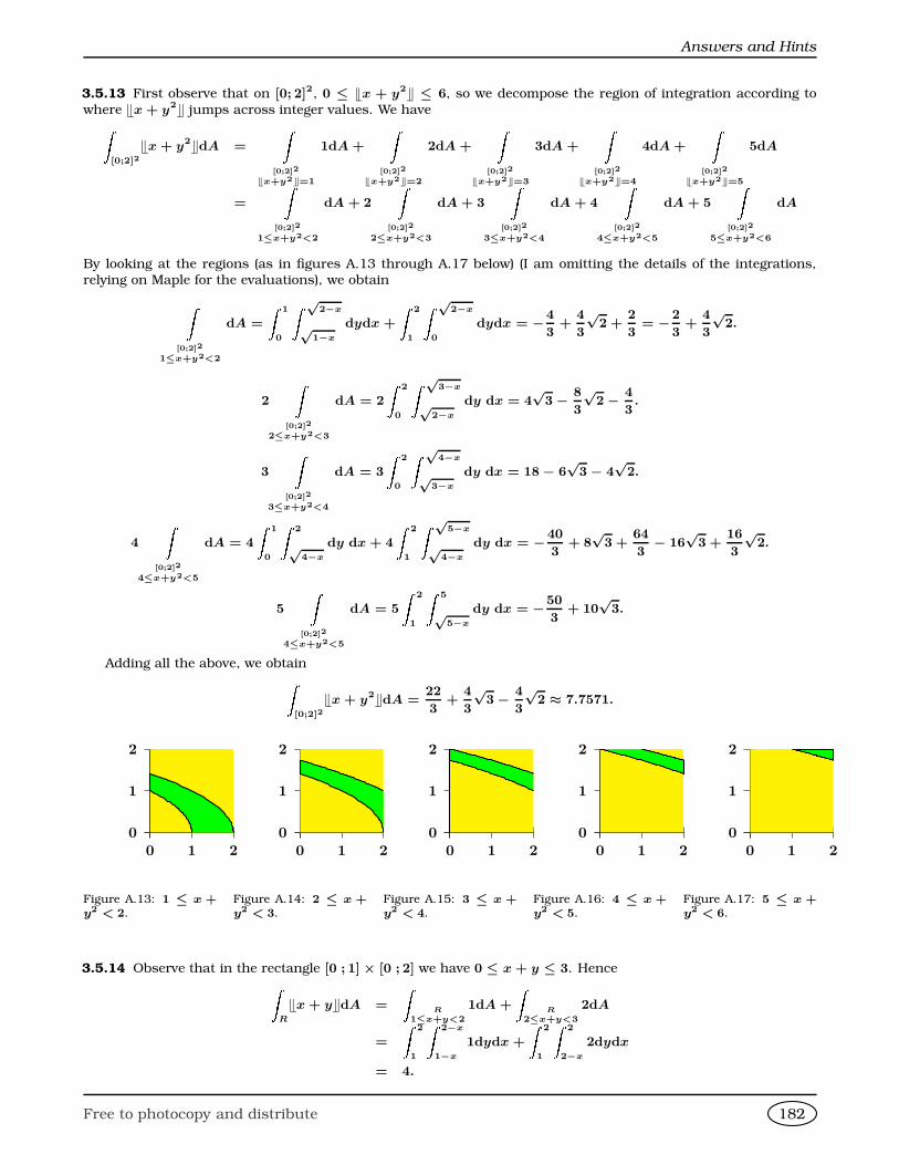
Answers and Hints
3.5.13 First observe that on [0; 2]2, 0 ≤ Tx + y2U ≤ 6, so we decompose the region of integration according to
where Tx + y2U jumps across integer values. We haveZ[0;2]2
Tx + y2UdA =
Z[0;2]2
Tx+y2U=1
1dA +
Z[0;2]2
Tx+y2U=2
2dA +
Z[0;2]2
Tx+y2U=3
3dA +
Z[0;2]2
Tx+y2U=4
4dA +
Z[0;2]2
Tx+y2U=5
5dA
=
Z[0;2]2
1≤x+y2<2
dA + 2
Z[0;2]2
2≤x+y2<3
dA + 3
Z[0;2]2
3≤x+y2<4
dA + 4
Z[0;2]2
4≤x+y2<5
dA + 5
Z[0;2]2
5≤x+y2<6
dA
By looking at the regions (as in figures A.13 through A.17 below) (I am omitting the details of the integrations,relying on Maple for the evaluations), we obtainZ
[0;2]2
1≤x+y2<2
dA =
Z 1
0
Z √2−x
√1−x
dydx +
Z 2
1
Z √2−x
0
dydx = −4
3+
4
3
√2 +
2
3= −2
3+
4
3
√2.
2
Z[0;2]2
2≤x+y2<3
dA = 2
Z 2
0
Z √3−x
√2−x
dy dx = 4√
3− 8
3
√2− 4
3.
3
Z[0;2]2
3≤x+y2<4
dA = 3
Z 2
0
Z √4−x
√3−x
dy dx = 18− 6√
3− 4√
2.
4
Z[0;2]2
4≤x+y2<5
dA = 4
Z 1
0
Z 2
√4−x
dy dx + 4
Z 2
1
Z √5−x
√4−x
dy dx = −40
3+ 8√
3 +64
3− 16
√3 +
16
3
√2.
5
Z[0;2]2
4≤x+y2<5
dA = 5
Z 2
1
Z 5
√5−x
dy dx = −50
3+ 10
√3.
Adding all the above, we obtainZ[0;2]2
Tx + y2UdA =22
3+
4
3
√3− 4
3
√2 ≈ 7.7571.
0
1
2
0 1 2
Figure A.13: 1 ≤ x +y2 < 2.
0
1
2
0 1 2
Figure A.14: 2 ≤ x +y2 < 3.
0
1
2
0 1 2
Figure A.15: 3 ≤ x +y2 < 4.
0
1
2
0 1 2
Figure A.16: 4 ≤ x +y2 < 5.
0
1
2
0 1 2
Figure A.17: 5 ≤ x +y2 < 6.
3.5.14 Observe that in the rectangle [0 ; 1] × [0 ; 2] we have 0 ≤ x + y ≤ 3. HenceZR
Tx + yUdA =
ZR
1≤x+y<2
1dA +
ZR
2≤x+y<3
2dA
=
Z 2
1
Z 2−x
1−x
1dydx +
Z 2
1
Z 2
2−x
2dydx
= 4.
Free to photocopy and distribute 182
Appendix A
3.5.15
Z 1
0
Z √4−x2
√1−x2
xdydx +
Z 2
1
Z √4−x2
0
xdydx =7
3.
3.5.16
Z 1
0
Z 3
−2
xdxdy +
Z 2
1
Z −1
−2
xdxdy +
Z 2
1
Z 1
0
xdxdy +
Z 2
1
Z 3
2
xdxdy = 7.
3.5.17 Exchanging the order of integration,Z π/2
0
Z y
0
cos y
ydxdy =
Z π/2
0
cos ydy = 1.
3.5.18 Upon splitting the domain of integration, we find that the integral equalsZ 2
1
Z y2
y
sinπx
2ydx
dy =
Z 2
1
−2y
πcos
πx
2y
y2
y
dy
= −Z 2
1
−2y
πcos
πy
2dy
=4(π + 2)
π3,
upon integrating by parts.
3.5.19 The integral is 0. Observe that if (x, y) ∈ D then (−x, y) ∈ D. Also, f(−x, y) = −f(x, y).
3.5.20
Z 2/√
5
−2/√
5
Z 12
√4−y2
− 12
√4−y2
dxdy =8
5+ 4 arcsin
√5
5
.
3.5.21 The integral equals ZD
xydA =
Z 1
0
Z 1− x
1 + x
0
xy dy
dx
=
Z 1
0
1
2x
1− x
1 + x
2
dx
=
Z 2
1
(t − 1)(t − 2)2
t2dt
= 4 loge 2− 11
4.
3.5.22 Using integration by parts,ZD
loge(1 + x2 + y)dA =
Z 1
0
Z 1−x2
0
loge(1 + x2 + y) dy
dx
=
Z 1
0
(2 loge(2)− 1− loge(1 + x2))dx
+
Z 1
0
(−x2 loge(1 + x2) + x2) dx
=2
3loge 2 +
8
9− π
3.
3.5.23
Z 2
0
Z √4−y2
√2y−y2
xdxdy = 2.
3.5.25 Let
D1 = (x, y) ∈ R2| − 1 ≤ x ≤ 1, x ≤ y,
D2 = (x, y) ∈ R2| − 1 ≤ x ≤ 1, x > y.
Then D = D1 ∪ D2, D1 ∩ D2 = ∅ and soZD
f(x, y)dxdy =
ZD1
f(x, y)dxdy +
ZD2
f(x, y)dxdy.
Free to photocopy and distribute 183
Answers and Hints
By symmetry, ZD1
f(x, y)dxdy =
ZD2
f(x, y)dxdy,
and so ZD
f(x, y)dxdy = 2
ZD1
f(x, y)dxdy
= 2
Z 1
−1
Z 1
x
(y − x) dy
dx
=
Z 1
−1
(1 − 2x + x2) dx
=8
3.
3.5.26 The line joining A, and B has equation y = −x−2, line joining B, and C has equation y = −7x+10, and
line joining A, and C has equation y = 2x + 1. We split the triangle along the vertical line x = 1, and integratefirst with respect to y. The desired integral is thenZ
D
(2x + 3y + 1) dxdy =
Z 1
−1
Z 2x+1
−x−2
(2x + 3y + 1)dy
dx
+
Z 2
1
Z −7x+10
−x−2
(2x + 3y + 1)dy
dx
=
Z 1
−1
21
2x2 + 9x − 3
2
dx
+
Z 2
1
60x2 − 198x + 156
dx
= 4− 1
= 3.
3.5.27 Since f is positive and decreasing,Z 1
0
Z 1
0
f(x)f(y)(y − x)(f(x) − f(y))dxdy ≥ 0,
from where the desired inequality follows.
3.5.28 The domain of integration is a triangle. The integral equalsZD
xy(x + y)dxdy =
Z 1
0
Z 1−x
0
xy(x + y) dy
dx
=
Z 1
0
x
x
y2
2+
y3
3
1−x
0
dx
=
Z 1
0
x
x(1− x)2
2+
(1 − x)3
3
dx
=1
30.
3.5.29 For t ∈ [0; 1], first argue that
Z 1
0
f(x)dx ≥ (1− t)f(t) ≥ f(t) − t. HenceZ 1
0
Z 1
0
(f(x)dx) dy ≥Z 1
0
(f g)(y)dy −Z 1
0
g(y)dy.
Since
Z 1
0
Z 1
0
f(x)dxdy =
Z 1
0
f(x)dx, the desired inequality is established.
3.5.30 Put f(x, y) = xy + y2. If I, II, III, IV stand for the intersection of the region with each quadrant, thenZII
f(x, y)dxdy =
ZII
f(−x, y)d(−x)dy = −ZI
f(x, y)dxdy,
Free to photocopy and distribute 184
Appendix AZIV
f(x, y)dxdy =
ZIV
f(x,−y)dxd(−y) = −ZI
f(x, y)dxdy,
and ZIII
f(x, y)dxdy =
ZIII
f(−x,−y)d(−x)d(−y) = +
ZI
f(x, y)dxdy.
Thus ZS
(xy + y2)dxdy =
ZI
f(x, y)dxdy +
ZII
f(x, y)dxdy +
ZIII
f(x, y)dxdy +
ZIV
f(x, y)dxdy
=
ZI
f(x, y)dxdy −ZI
f(x, y)dxdy +
ZI
f(x, y)dxdy −ZI
f(x, y)dxdy
= 0.
3.5.31 We split the rectangle [0; a]× [0; b] into two triangles, depending on whether bx < ay or bx ≥ ay. HenceZ a
0
Z b
0
emax(b2x2,a2y2) dydx =
Zbx<ay
emax(b2x2,a2y2) dydx +
Zbx≥ay
emax(b2x2,a2y2) dydx
=
Zbx<ay
ea2y2
dydx +
Zbx≥ay
eb2x2
dydx
=
Z b
0
Z ay/b
0
ea2y2
dxdy +
Z a
0
Z bx/a
0
ea2y2
dydx
=
Z b
0
ayea2y2
bdy +
Z a
0
bxea2y2
adx
=ea2b2 − 1
2ab+
ea2b2 − 1
2ab
=ea2b2 − 1
ab.
3.5.32 Observe that x ≥ 1
2(x + y)2 ≥ 0. Hence we may take the positive square root giving y ≤
√2x − x. Since
y ≥ 0, we must have√
2x − x ≥ 0 which means that x ≤ 2. The integral equalsZ 2
0
Z √2x−x
0
√xydy
dx =
2
3
Z 2
0
√x(√
2x − x)3/2dx
=4
3
Z √2
0
u2(u√
2− u2)3/2du
=1
6
Z 1
−1
(1 − v2)3/2(1 + v)2dv
=1
6
Z π/2
−π/2
cos4 θ(1 + sin2 θ)dθ
=7π
96.
3.5.33 Observe that Z a
0
sin 2πx dx =
(0 if a is an integer1
2π(1− cos 2πa) if a is not an integer
Thus Z a
0
sin 2πx dx = 0 ⇐⇒ a is an integer.
NowNX
k=1
ZRk
sin 2πx sin 2πy dxdy = 0
since at least one of the sides of each Rk is an integer. SinceZR
sin 2πx sin 2πy dxdy =
NXk=1
ZRk
sin 2πx sin 2πy dxdy,
we deduce that at least one of the sides of R is an integer, finishing the proof.
Free to photocopy and distribute 185
Answers and Hints
3.5.34 We have Z 1
0
Z 1
0
· · ·Z 1
0
(x1x2 · · · xn)dx1dx2 . . . dxn =
nYk=1
Z 1
0
xkdxk
=
nYk=1
1
2=
1
2n.
3.5.35 This is Z 1
0
Z 1
0
· · ·Z 1
0
nX
k=1
xk
dx1dx2 . . . dxn =
nXk=1
Z 1
0
Z 1
0
· · ·Z 1
0
xkdx1dx2 . . . dxn
=
nXk=1
1
2
=n
2.
3.5.41 The integral equals ZD
1
(x + y)4dxdy =
Z 3
1
Z 4−x
1
dy
(x + y)4dy
dx
=
Z 3
1
h−1
3(x + y)−3
i4−x
1dx
=1
3
Z 3
1
1
(1 + x)3− 1
64
dx
=1
48.
3.5.45 The integral equalsZD
xdxdy =
Z 2/3
−1
Z x+1
0
dy
x dx +
Z 4
2/3
Z 2− x2
0
dy
x dx
=
Z 2/3
−1
x(x + 1) dx +
Z 4
2/3
x2− x
2
dx
=275
54.
3.5.46 Make the change of variables xk = 1− yk . Then
I =
Z 1
0
Z 1
0
· · ·Z 1
0
cos2 π
2n(x1 + x2 + · · ·+ xn)
dx1 dx2 . . . dxn
equals Z 1
0
Z 1
0
· · ·Z 1
0
sin2 π
2n(y1 + y2 + · · · + yn)
dy1 dy2 . . . dyn .
Since sin2 t + cos2 t = 1, we have 2I = 1, and so I =1
2.
3.6.1 ➊ Put x =u + v
2and y =
u − v
2. Then x + y = u and x − y. Observe that D′ is the triangle in the uv
plane bounded by the lines u = 0, u = 1, v = u, v = −u. Its image under Φ is the triangle bounded by theequations x = 0, y = 0, x + y = 1. Clearly also
dx ∧ dy =1
2du ∧ dv.
➋ From the above ZD
(x + y)2ex2−y2
dA =1
2
ZD′
u2euvdudv
=1
2
Z 1
0
Z u
−u
u2euvdudv
=1
2
Z 1
0
u(eu2 − e−u2
)du
=1
4(e + e−1 − 2).
Free to photocopy and distribute 186
Appendix A
3.6.4 Here we argue that
du = ydx + xdy,
dv = −2xdx + 2ydy.
Taking the wedge product of differential forms,
du ∧ dv = 2(y2 + x2)dx ∧ dy.
Hence
f(x, y)dx ∧ dy = (y4 − x4)1
2(y2 + x2)du ∧ dv
=1
2(y2 − x2)du ∧ dv
=v
2du ∧ dv
The region transforms into
∆ = [a; b]× [0; 1].
The integral becomes ZD
f(x, y)dx ∧ dy =
Z∆
v du ∧ dv
=1
2
Z b
a
du
Z 1
0
v dv
=
b − a
4.
3.6.5 ➊ Formally, Z 1
0
Z 1
0
dxdy
1− xy=
Z 1
0
Z 1
0
(1 + xy + x2y2 + x3y3 + · · · )dxdy
=
Z 1
0
y +
xy2
2+
x2y3
3+
x3y4
4+ · · ·
1
0
dx
=
Z 1
0
(1 +x
2+
x2
3+
x3
4+ · · · )dx
= 1 +1
22+
1
32+
1
42+ · · ·
➋ This change of variables transforms the square [0; 1] × [0; 1] in the xy plane into the square with verticesat (0, 0), (1, 1), (2, 0), and (1,−1) in the uv plane. We will split this region of integration into two disjointtriangles: T1 with vertices at (0, 0), (1, 1), (1,−1), and T2 with vertices at (1,−1), (1, 1), (2, 0). Observe
that
dx ∧ dy =1
2du ∧ dv,
and that u + v = 2x, u − v = 2y and so 4xy = u2 − v2. The integral becomesZ 1
0
Z 1
0
dxdy
1− xy=
1
2
ZT1∪T2
du ∧ dv
1− u2−v2
4
= 2
Z 1
0
Z u
−u
dv
4− u2 + v2
du + 2
Z 2
1
Z 2−u
u−2
dv
4− u2 + v2
du,
as desired.
➌ This follows by using the identity Z t
0
dω
1 + Ω2= arctan t.
➍ This is straightforward but tedious!
3.7.1 The integral in Cartesian coordinates isZ √15
1
Z √16−y2
1
xydxdy =1
2
Z Z √15
1
15y − y3dy
=49
2.
Free to photocopy and distribute 187
Answers and Hints
The integral in polar coordinates isZ π4
arcsin 14
Z 4
1/ sin θ
r3 sin θ cos θdrdθ +
Z arccos 14
π4
Z 4
1/ cos θ
r3 sin θ cos θdrdθ =1
4
Z π4
arcsin 14
44 − 1
sin4 θ
sin θ cos θdθ
+1
4
Z arccos 14
π4
44 − 1
cos4 θ
sin θ cos θdθ
=44
4
Z arccos 14
arcsin π4
sin θ cos θdθ
−1
4
Z π4
arcsin 14
(cot θ)(csc2 θ)dθ
−1
4
Z arccos 14
π4
(tan θ)(sec2 θ)dθ
= 28− 7
4− 7
4
=49
2
3.7.2 Using polar coordinates,ZD
x2 − y2dxdy =
Z π/2
−π/2
Z 2 cos θ
0
ρ3 dρ
(cos2 θ − sin2 θ)dθ
= 8
Z π/2
0
cos4 θ(cos2 θ − sin2 θ) dθ
= π.
3.7.3 Using polar coordinates,ZD
√xydxdy = 4
Z π/4
0
Z √sin 2θ
0
ρp
ρ2 cos θ sin θ dρ
dθ
=4
3
Z π/4
0
(√
sin 2θ)3√
cos θ sin θ dθ
=4
3√
2
Z π/4
0
sin2 2θ dθ
=π√
2
12.
3.7.4 Using x = aρ cos θ, y = bρ sin θ, the integral becomes
(ab)
Z 2π
0
a3 cos3 θ + b3 sin3 θdθ
Z 1
0
ρ4dρ
=
2
15(ab)(a3 + b3).
3.7.8 Using polar coordinates, ZD
f(x, y)dA =
Z π/6
0
Z 1
2 sin θ
ρ2 dρ
dθ
=1
3
Z π/6
0
(1− 8 sin3 θ) dθ
=π
18− 16
9+√
3.
3.7.9 Using polar coordinates the integral becomesZ π/2
0
Z 2 cos θ
0
ρ4dρ
cos2 θ sin θdθ =
4
5.
3.7.11 Using polar coordinates the integral becomesZ π/4
−π/4
Z 2 cos θ
1/ cos θ
1
ρ3dρ
dθ =
Z π/4
0
cos2 θ − sec2 θ
4
dθ =
π
8.
Free to photocopy and distribute 188
Appendix A
3.7.12 Put
D′ = (x, y) ∈ R2 : y ≥ x, x2 + y2 − y ≤ 0, x2 + y2 − x ≤ 0.
Then the integral equals
2
ZD′
(x + y)2dxdy.
Using polar coordinates the integral equals
2
Z π/2
π/4
(cos θ + sin θ)2Z cos θ
0
ρ3dρ
dθ =
1
2
Z π/2
π/4
cos4 θ(1 + 2 sin θ cos θ)dθ
=3π
64− 5
48.
3.7.13 Observe that D = D2 \ D1 where D2 is the disk limited by the equation x2 + y2 = 1 and D1 is the disklimited by the equation x2 + y2 = y. HenceZ
D
dxdy
(1 + x2 + y2)2=
ZD2
dxdy
(1 + x2 + y2)2−Z
D1
dxdy
(1 + x2 + y2)2.
Using polar coordinates we haveZD2
dxdy
(1 + x2 + y2)2=
Z 2π
0
Z 1
0
ρ
(1 + ρ2)2dρdθ =
π
2
and ZD1
dxdy
(1 + x2 + y2)2= 2
Z π/2
0
Z sin θ
0
ρ
(1 + ρ2)2dρdθ =
Z π/2
0
sin2 θdθ
1 + sin2 θ
=
Z +∞
0
dt
t2 + 1− dt
2t2 + 1=
π
2− π√
2
4.
(We evaluated this last integral using t = tan θ) Finally, the integral equals
π
2−
π
2− π√
2
4
=
π√
2
4.
3.7.14 We have
2xdx = cos θdρ − ρ sin θdθ, 2ydy = sin θdρ + ρ cos θdθ,
whence4xydx ∧ dy = ρdρ ∧ dθ.
It follows that
x3y3p
1− x4 − y4 dx ∧ dy =1
4(x2y2)(
p1− x4 − y4)(4xy dx ∧ dy)
=1
4(ρ3 cos θ sin θ
p1− ρ2)dρ ∧ dθ
Observe thatx4 + y4 ≤ 1 =⇒ ρ2 cos2 θ + ρ2 sin2 θ ≤ 1 =⇒ ρ ≤ 1.
Since the integration takes place on the first quadrant, we have 0 ≤ θ ≤ π/2. Hence the integral becomesZ π/2
0
Z 1
0
1
4(ρ3 cos θ sin θ
p1− ρ2)dρdθ =
1
4
Z π/2
0
cos θ sin θdθ
Z 1
0
ρ3p
1− ρ2dρ
=
1
4· 12· 2
15
=1
60.
3.7.15 ➊ Using polar coordinates
Ia =
Z 2π
0
Z a
0
ρe−ρ2
dρ
dθ = π(1− e−a2
).
➋ The domain of integration of Ja is a square of side 2a centred at the origin. The respective domains ofintegration of Ia and Ia
√2 are the inscribed and the exscribed circles to the square.
➌ First observe that
Ja =
Z a
−a
e−x2
dx
2
.
Since both Ia and Ia√
2 tend to π as a→ +∞, we deduce that Ja → π. This gives the result.
Free to photocopy and distribute 189
Answers and Hints
3.7.16 Z4≤x2+y2≤16
1
x2 + xy + y2dA =
Z 2π
0
Z 4
2
r
r2 + r2 sin θ cos θdrdθ
=
Z 2π
0
Z 4
2
1
r(1 + sin θ cos θ)drdθ
=
Z 2π
0
dθ
1 + sin θ cos θ
Z 4
2
dr
r
=
Z 2π
0
dθ
1 + sin θ cos θ
log 2
= 2
Z 2π
0
dθ
2 + sin 2θ
log 2
= 4
Z π
0
dθ
2 + sin 2θ
log 2
= 4I log 2,
so the problem reduces to evaluate I =
Z π
0
dθ
2 + sin 2θ. To find this integral, we now use what has been dubbed
as “the world’s sneakiest substitution”1: we put tan θ = t. In so doing we have to pay attention to the fact that
θ 7→ tan θ is not continuous on [0; π], so we split the interval of integration into two pieces, [0; π] = [0;π
2]∪]
π
2; π].
Then sin 2θ =2t
1 + t2, cos 2θ =
1− t2
1 + t2, dθ =
dt
1 + t2. HenceZ π
0
dθ
2 + sin 2θ=
Z π/2
0
dθ
2 + sin 2θ+
Z π
π/2
dθ
2 + sin 2θ
=
Z +∞
0
dt1+t2
2 + 2t1+t2
+
Z 0
−∞
dt1+t2
2 + 2t1+t2
=
Z +∞
0
dt
2(t2 + t + 1)+
Z 0
−∞
dt
2(t2 + t + 1)
=2
3
Z +∞
0
dt
( 2t√3
+ 1√3)2 + 1
+2
3
Z 0
−∞
dt
( 2t√3
+ 1√3)2 + 1
=
√3
3
+∞
0arctan
2t√
3
3+
√3
3
+
√3
3
0−∞
arctan
2t√
3
3+
√3
3
=
√3
3
π
2− π
6
+
√3
3
π
6−−π
2
=
π√
3
3.
We conclude that Z4≤x2+y2≤16
1
x2 + xy + y2dA =
4π√
3 log 2
3.
3.7.17 Recall from formula 1.14 that the area enclosed by a simple closed curve Γ is given by
1
2
ZΓ
xdy − ydx.
Using polar coordinates
xdy − ydx = (ρ cos θ)(sin θdρ + ρ cos θdθ) − (ρ sin θ)(cos θdρ − ρ sin θdθ)
= ρ2dθ.
Parametrise the curve enclosing the region by polar coordinates so that the region is tangent to the polar axis atthe origin. Let the equation of the curve be ρ = f(θ). The area of the region is then given by
1
2
Z π
0
ρ2dθ =1
2
Z π
0
(f(θ))2dθ =1
2
Z π/2
0
((f(θ))2 + (f(θ + π/2))2)dθ.
By the Pythagorean Theorem, the integral above is the integral of the square of the chord in question. If no twopoints are farther than 2 units, their squares are no farther than 4 units, and so the area
<1
2
Z π/2
0
4dθ = π,
1by Michael Spivak, whose Calculus book I recommend greatly.
Free to photocopy and distribute 190
Appendix A
a contradiction.
3.7.18 Let I(S) denote the integral sought over a region S. Since D(x, y) = 0 inside R, I(R) = A. Let L be aside of R with length l and let S(L ) be the half strip consisting of the points of the plane having a point on L as
nearest point of R. Set up coordinates uv so that u is measured parallel to L and v is measured perpendicular toL. Then
I(S(L )) =
Z l
0
Z +∞
0
e−v dudv = l.
The sum of these integrals over all the sides of R is L.If V is a vertex of R, the points that have V as nearest from R lie inside an angle S(V ) bounded by the rays
from V perpendicular to the edges meeting at V . If α is the measure of that angle, then using polar coordinates
I(S(V )) =
Z α
0
Z +∞
0
ρe−ρ dρdθ = α.
The sum of these integrals over all the vertices of R is 2π. Assembling all these integrals we deduce the result.
3.8.1 We have ZE
zdV =
Z 1
0
Z 1−y
0
Z 1−z
0
zdxdzdy
=
Z 1
0
Z 1−y
0
z − z2dzdy
=
Z 1
0
(1− y)2
2− (1− y)3
3dy
=(1− y)4
12− (1− y)3
6
10
= =1
6.
3.8.3 Let A = (1, 1, 1), B = (1, 0, 0), C = (0, 0, 1), and O = (0, 0, 0). We have four planes passing through each
triplet of points:
P1 : A, B, C, x − y + z = 1
P2 : A, B, O z = y
P3 : A, C, O x = y
P4 : B, C, O y = 0.
Using the order of integration dzdxdy, z sweeps from P2 to P1, so the limits are z = y to z = 1 − x + y. Theprojection of the solid on the xy plane produces the region bounded by the lines x = 0, x = 1 and x = y on thefirst quadrant of the xy-plane. ThusZ 1
0
Z x
0
Z 1−x+y
y
dzdydx =
Z 1
0
Z x
0
(1− x)dydx
=
Z 1
0
x − x2 dx
=
x2
2− x3
3
10
=1
6.
We use the same limits of integration as in the previous integral. We haveZ 1
0
Z x
0
Z 1−x+y
y
xdzdydx =
Z 1
0
Z x
0
(x − x2)dydx
=
Z 1
0
x2 − x3 dx
=
x3
3− x4
4
10
=1
12.
3.8.4 We have ZE
xdV =
Z 3
0
Z √9−x2
0
Z y/3
0
xdzdydx =27
8.
Free to photocopy and distribute 191
Answers and Hints
3.8.5 The desired integral isZ 1
0
Z 1
0
Z ∞
0
dxdydz
(1 + x2z2)(1 + y2z2)=
Z 1
0
Z 1
0
Z ∞
0
1
x2 − y2
x2
1 + x2z2− y2
1 + y2z2
dxdydz
=
Z 1
0
Z 1
0
1
x2 − y2(x arctan(xz)− y arctan(yz))
z=∞
z=0
dxdy
=
Z 1
0
Z 1
0
π(x − y)
2(x2 − y2)dxdy
=
Z 1
0
Z 1
0
π
2(x + y)dxdy
=π
2
Z 1
0
log(y + 1)− log ydy
=π
2· ((y + 1) log(y + 1)− (y + 1)− y log y + y)
10
= π log 2.
3.9.1 Cartesian: Z 1
−1
Z √1−y2
−√
1−y2
Z √x2+y2
x2+y2
dzdxdy.
Cylindrical: Z 1
0
Z 2π
0
Z r
r2
rdzdθdr.
Spherical: Z π/2
π/4
Z 2π
0
Z (cos φ)/(sin φ)2
0
r2 sin φdrdθdφ.
The volume isπ
3.
3.9.2
1. Since x2 + y2 ≤ z ≤p
4− x2 − y2, we start our integration with the z-variable. Observe that if (x, y, z) ison the intersection of the surfaces then
z2 + z = 4 =⇒ z =−1±
√17
2.
Since x2 + y2 + z2 = 4 =⇒ −2 ≤ z ≤ 2, we must have z =
√17− 1
2only. The projection of the circle of
intersection of the paraboloid and the sphere onto the xy-plane satisfies the equation
z2 + z = 4 =⇒ x2 + y2 + (x2 + y2)2 = 4 =⇒ x2 + y2 =
√17− 1
2,
a circle of radius
r√17− 1
2. The desired integral is thusZ È√
17−12
−È√
17−12
Z È√17−12
−x2
−È√
17−12
−x2
Z √4−x2−y2
x2+y2
xdzdydx.
2. The z-limits remain the same as in the Cartesian coordinates, but translated into cylindrical coordinates,
and so r2 ≤ z ≤p
4− r2. The projection of the intersection circle onto the xy-plane is again a circle with
centre at the origin and radius
r√17− 1
2. The desired integralZ 2π
0
Z È√17−12
0
Z √4−r2
r2
r2 cos θdzdrdθ.
Free to photocopy and distribute 192
Appendix A
3. Observe that
z = x2 + y2 =⇒ r cos φ = r2(cos θ)2(sin φ)2 + r2(sin θ)2(sin φ)2 =⇒ r ∈ 0, (csc φ)(cot φ).
It is clear that the limits of the angle θ are from θ = 0 to θ = 2π. The angle φ starts at φ = 0. Now,
z = r cos φ =⇒ cos φ =
√17− 1
22
=⇒ φ = arccos
√17− 1
4
The desired integral Z 2π
0
Z arccos
√17− 1
4
0
Z 2
(csc φ)(cot φ)
r3 cos θ sin2 φdrdφdθ.
Perhaps it is easiest to evaluate the integral using cylindrical coordinates. We obtainZ 2π
0
Z É√17− 1
2
0
Z √4−r2
r2
r2 cos θdzdrdθ = 0,
a conclusion that is easily reached, since the integrand is an odd function of x and the domain of integration is
symmetric about the origin in x.
3.9.3 Cartesian: Z √3
−√
3
Z √3−y2
−√
3−y2
Z √4−x2−y2
1
dzdxdy.
Cylindrical: Z √3
0
Z 2π
0
Z √4−r2
1
rdzdθdr.
Spherical: Z π/3
0
Z 2π
0
Z 2
1/ cos φ
r2 sin φdrdθdφ.
The volume is5π
3.
3.9.5 We have ZE
ydV =
Z 2π
0
Z 2
1
Z 2+r cos θ
0
r2 sin θdzdrdθ = 0.
3.9.7π
96
3.9.8π
14
3.9.9 We put
x = ρ cos θ sin φ sin t; y = ρ sin θ sin φ sin t; u = ρ cos φ sin t; v = ρ cos t.
Upon using sin2 a + cos2 a = 1 three times,
x2 + y2 + u2 + v2 = r2 cos2 θ sin2 φ sin2 t + r2 sin2 θ sin2 φ sin2 t + r2 cos2 φ sin2 t + r2 cos2 t
= r2 cos2 θ sin2 φ + r2 sin2 θ sin2 φ + r2 cos2 φ
= r2 cos2 θ + r2 sin2 θ
= r2.
Now,
dx = cos θ sin φ sin tdr − ρ sin θ sin φ sin tdθ + ρ cos θ cos φ sin tdφ + ρ cos θ sin φ cos tdt
dy = sin θ sin φ sin tdr + ρ cos θ sin φ sin tdθ + ρ sin θ cos φ sin tdφ + ρ sin θ sin φ cos tdt
du = cos φ sin tdr − ρ sin φ sin tdφ + ρ cos φ cos tdt
dv = cos tdr − ρ sin tdt
.
Free to photocopy and distribute 193
Answers and Hints
After some calculation,
dx ∧ dy ∧ du ∧ dv = r3 sin φ sin2 tdr ∧ dφ ∧ dθ ∧ dt.
Therefore ZZZZx2+y2+u2+v2≤1
ex2+y2+u2+v2
dxdydudv =
Z π
0
Z 2π
0
Z π
0
Z 1
0
r3er2
sin φ sin2 tdrdφdθdt
=
Z 1
0
r3er2
dr
Z 2π
0
dθ
Z π
0
sin φdφ
Z π
0
sin2 tdt
=
1
2
(2π)(2)
π
2
= π2.
3.9.10 We make the change of variables
u = x + y + z =⇒ du = dx + dy + dz,
uv = y + z =⇒ udv + vdu = dy + dz,
uvw = z =⇒ uvdw + uwdv + vwdu = dz.
This gives
x = u(1− v),
y = uv(1− w),
z = uvw,
u2v du ∧ dv ∧ dw = dx ∧ dy ∧ dz.
To find the limits of integration we observe that the limits of integration using dx ∧ dy ∧ dz are
0 ≤ z ≤ 1, 0 ≤ y ≤ 1− z, 0 ≤ x ≤ 1− y − z.
This translates into
0 ≤ uvw ≤ 1, 0 ≤ uv − uvw ≤ 1− uvw, 0 ≤ u − uv ≤ 1− uv + uvw − uvw.
Thus
0 ≤ uvw ≤ 1, 0 ≤ uv ≤ 1, 0 ≤ u ≤ 1,
which finally give
0 ≤ u ≤ 1, 0 ≤ v ≤ 1, 0 ≤ w ≤ 1.
The integral sought is then, using the fact that for positive integers m, n one hasZ 1
0
xm(1− x)n dx =m!n!
(m + n + 1)!,
we deduce, Z 1
0
Z 1
0
Z 1
0
u20v18w8(1− u)4(1− v)(1− w)9 dudvdw,
which in turn isZ 1
0
u20(1− u)4du
Z 1
0
v18(1 − v)dv
Z 1
0
w8(1− w)9dw
=
1
265650· 1
380· 1
437580
which is
=1
44172388260000.
3.10.1 We parametrise the surface by letting x = u, y = v, z = u + v2. Observe that the domain D of Σ is thesquare [0; 1]× [0; 2]. Observe that
dx ∧ dy = du ∧ dv,
dy ∧ dz = −du ∧ dv,
dz ∧ dx = −2vdu ∧ dv,
and so d2x = p
2 + 4v2du ∧ dv.
Free to photocopy and distribute 194
Appendix A
The integral becomes ZΣ
yd2x
=
Z 2
0
Z 1
0
vp
2 + 4v2dudv
=
Z 1
0
du
Z 2
0
yp
2 + 4v2dv
=
13√
2
3.
3.10.2 Using x = r cos θ, y = r sin θ, 1 ≤ r ≤ 2, 0 ≤ θ ≤ 2π, the surface area is
√2
Z 2π
0
Z 2
1
rdrdθ = 3π√
2.
3.10.3 We use spherical coordinates, (x, y, z) = (cos θ sin φ, sin θ sin φ, cos φ). Here θ ∈ [0; 2π] is the latitude
and φ ∈ [0; π] is the longitude. Observe that
dx ∧ dy = sin φ cos φdφ ∧ dθ,
dy ∧ dz = cos θ sin2 φdφ ∧ dθ,
dz ∧ dx = − sin θ sin2 φdφ ∧ dθ,
and so d2x = sin φdφ ∧ dθ.
The integral becomes ZΣ
x2d2x
=
Z 2π
0
Z π
0
cos2 θ sin3 φdφdθ
=4π
3.
3.10.4 Put x = u, y = v, z2 = u2 + v2. Then
dx = du, dy = dv, zdz = udu + vdv,
whence
dx ∧ dy = du ∧ dv, dy ∧ dz = −u
zdu ∧ dv, dz ∧ dx = −v
zdu ∧ dv,
and so d2x =
È(dx ∧ dy)2 + (dz ∧ dx)2 + (dy ∧ dz)2
=
É1 +
u2 + v2
z2du ∧ dv
=√
2 du ∧ dv.
Hence ZΣ
zd2x
= Zu2+v2≤1
pu2 + v2
√2 dudv =
√2
Z 2π
0
Z 1
0
ρ2 dρdθ =2π√
2
3.
3.10.5 If the egg has radius R, each slice will have height 2R/n. A slice can be parametrised by 0 ≤ θ ≤ 2π,
φ1 ≤ φ ≤ φ2, with
R cos φ1 − R cos φ2 = 2R/n.
The area of the part of the surface of the sphere in slice isZ 2π
0
Z φ2
φ1
R2 sin φdφdθ = 2πR2(cos φ1 − cos φ2) = 4πR2/n.
This means that each of the n slices has identical area 4πR2/n.
3.10.6 We project this plane onto the coordinate axes obtainingZΣ
xydydz =
Z 6
0
Z 3−z/2
0
(3− y − z/2)ydydz =27
4,
Free to photocopy and distribute 195
Answers and Hints
−ZΣ
x2dzdx = −Z 3
0
Z 6−2x
0
x2dzdx = −27
2,Z
Σ
(x + z)dxdy =
Z 3
0
Z 3−y
0
(6− x − 2y)dxdy =27
2,
and hence ZΣ
xydydz − x2dzdx + (x + z)dxdy =27
4.
3.11.1 Evaluating this directly would result in evaluating four path integrals, one for each side of the square. Wewill use Green’s Theorem. We have
dω = d(x3y) ∧ dx + d(xy) ∧ dy
= (3x2ydx + x3dy) ∧ dx + (ydx + xdy) ∧ dy
= (y − x3)dx ∧ dy.
The region M is the area enclosed by the square. The integral equalsIC
x3ydx + xydy =
Z 2
0
Z 2
0
(y − x3)dxdy
= −4.
3.11.2 We have
➊ LAB is y = x; LAC is y = −x, and LBC is clearly y = −1
3x +
4
3.
➋ We have ZAB
y2dx + xdy =
Z 1
0
(x2 + x)dx =5
6ZBC
y2dx + xdy =
Z −2
1
−1
3x +
4
3
2
− 1
3x
dx = −15
2ZCA
y2dx + xdy =
Z 0
−2
(x2 − x)dx =14
3
Adding these integrals we find I4
y2dx + xdy = −2.
➌ We have ZD
(1− 2y)dx ∧ dy =
Z 0
−2
Z −x/3+4/3
−x
(1− 2y)dy
dx
+
Z 1
0
Z −x/3+4/3
x
(1− 2y)dy
dx
= −44
27− 10
27
= −2.
3.11.6 Observe thatd(x2 + 2y3) ∧ dy = 2xdx ∧ dy.
Hence by the generalised Stokes’ Theorem the integral equalsZ(x−2)2+y2≤4
2xdx ∧ dy =
Z π/2
−π/2
Z 4 cos θ
0
2ρ2 cos θdρ ∧ dθ = 16π.
To do it directly, put x − 2 = 2 cos t, y = 2 sin t, 0 ≤ t ≤ 2π. Then the integral becomesZ 2π
0
((2 + 2 cos t)2 + 16 sin3 t)d2 sin t =
Z 2π
0
(8 cos t + 16 cos2 t
+8 cos3 t + 32 cos t sin3 t)dt
= 16π.
Free to photocopy and distribute 196
Appendix A
3.11.7 At the intersection path
0 = x2 + y2 + z2 − 2(x + y) = (2− y)2 + y2 + z2 − 4 = 2y2 − 4y + z2 = 2(y − 1)2 + z2 − 2,
which describes an ellipse on the yz-plane. Similarly we get 2(x − 1)2 + z2 = 2 on the xz-plane. We have
d (ydx + zdy + xdz) = dy ∧ dx + dz ∧ dy + dx ∧ dz = −dx ∧ dy − dy ∧ dz − dz ∧ dx.
Since dx ∧ dy = 0, by Stokes’ Theorem the integral sought is
−Z
2(y−1)2+z2≤2
dydz −Z
2(x−1)2+z2≤2
dzdx = −2π(√
2).
(To evaluate the integrals you may resort to the fact that the area of the elliptical region(x − x0)
2
a2+
(y − y0)2
b2≤ 1
is πab).
If we were to evaluate this integral directly, we would set
y = 1 + cos θ, z =√
2 sin θ, x = 2− y = 1− cos θ.
The integral becomesZ 2π
0
(1 + cos θ)d(1 − cos θ) +√
2 sin θd(1 + cos θ) + (1− cos θ)d(√
2 sin θ)
which in turn
=
Z 2π
0
sin θ + sin θ cos θ −√
2 +√
2 cos θdθ = −2π√
2.
Free to photocopy and distribute 197

GNU Free Documentation License
Version 1.2, November 2002Copyright c© 2000,2001,2002 Free Software Foundation, Inc.
51 Franklin St, Fifth Floor, Boston, MA 02110-1301 USA
Everyone is permitted to copy and distribute verbatim copies of this license document, but changing it is not allowed.
Preamble
The purpose of this License is to make a manual, textbook, or other functional and useful document “free” in the sense of freedom: to assure everyone the effective freedom to copy and redistributeit, with or without modifying it, either commercially or noncommercially. Secondarily, this License preserves for the author and publisher a way to get credit for their work, while not being consideredresponsible for modifications made by others.
This License is a kind of “copyleft”, which means that derivative works of the document must themselves be free in the same sense. It complements the GNU General Public License, which is a copyleftlicense designed for free software.
We have designed this License in order to use it for manuals for free software, because free software needs free documentation: a free program should come with manuals providing the same freedomsthat the software does. But this License is not limited to software manuals; it can be used for any textual work, regardless of subject matter or whether it is published as a printed book. We recommend thisLicense principally for works whose purpose is instruction or reference.
1. APPLICABILITY AND DEFINITIONSThis License applies to any manual or other work, in any medium, that contains a notice placed by the copyright holder saying it can be distributed under the terms of this License. Such a notice
grants a world-wide, royalty-free license, unlimited in duration, to use that work under the conditions stated herein. The “Document”, below, refers to any such manual or work. Any member of the publicis a licensee, and is addressed as “you”. You accept the license if you copy, modify or distribute the work in a way requiring permission under copyright law.
A “Modified Version” of the Document means any work containing the Document or a portion of it, either copied verbatim, or with modifications and/or translated into another language.A “Secondary Section” is a named appendix or a front-matter section of the Document that deals exclusively with the relationship of the publishers or authors of the Document to the Document’s
overall subject (or to related matters) and contains nothing that could fall directly within that overall subject. (Thus, if the Document is in part a textbook of mathematics, a Secondary Section may notexplain any mathematics.) The relationship could be a matter of historical connection with the subject or with related matters, or of legal, commercial, philosophical, ethical or political position regardingthem.
The “Invariant Sections” are certain Secondary Sections whose titles are designated, as being those of Invariant Sections, in the notice that says that the Document is released under this License. If asection does not fit the above definition of Secondary then it is not allowed to be designated as Invariant. The Document may contain zero Invariant Sections. If the Document does not identify any InvariantSections then there are none.
The “Cover Texts” are certain short passages of text that are listed, as Front-Cover Texts or Back-Cover Texts, in the notice that says that the Document is released under this License. A Front-CoverText may be at most 5 words, and a Back-Cover Text may be at most 25 words.
A “Transparent” copy of the Document means a machine-readable copy, represented in a format whose specification is available to the general public, that is suitable for revising the documentstraightforwardly with generic text editors or (for images composed of pixels) generic paint programs or (for drawings) some widely available drawing editor, and that is suitable for input to text formatters orfor automatic translation to a variety of formats suitable for input to text formatters. A copy made in an otherwise Transparent file format whose markup, or absence of markup, has been arranged to thwartor discourage subsequent modification by readers is not Transparent. An image format is not Transparent if used for any substantial amount of text. A copy that is not “Transparent” is called “Opaque”.
Examples of suitable formats for Transparent copies include plain ASCII without markup, Texinfo input format, LaTeX input format, SGML or XML using a publicly available DTD, and standard-conforming simple HTML, PostScript or PDF designed for human modification. Examples of transparent image formats include PNG, XCF and JPG. Opaque formats include proprietary formats that can beread and edited only by proprietary word processors, SGML or XML for which the DTD and/or processing tools are not generally available, and the machine-generated HTML, PostScript or PDF produced bysome word processors for output purposes only.
The “Title Page” means, for a printed book, the title page itself, plus such following pages as are needed to hold, legibly, the material this License requires to appear in the title page. For works informats which do not have any title page as such, “Title Page” means the text near the most prominent appearance of the work’s title, preceding the beginning of the body of the text.
A section “Entitled XYZ” means a named subunit of the Document whose title either is precisely XYZ or contains XYZ in parentheses following text that translates XYZ in another language. (HereXYZ stands for a specific section name mentioned below, such as “Acknowledgements”, “Dedications”, “Endorsements”, or “History”.) To “Preserve the Title” of such a section when you modify theDocument means that it remains a section “Entitled XYZ” according to this definition.
The Document may include Warranty Disclaimers next to the notice which states that this License applies to the Document. These Warranty Disclaimers are considered to be included by reference inthis License, but only as regards disclaiming warranties: any other implication that these Warranty Disclaimers may have is void and has no effect on the meaning of this License.
2. VERBATIM COPYINGYou may copy and distribute the Document in any medium, either commercially or noncommercially, provided that this License, the copyright notices, and the license notice saying this License
applies to the Document are reproduced in all copies, and that you add no other conditions whatsoever to those of this License. You may not use technical measures to obstruct or control the reading orfurther copying of the copies you make or distribute. However, you may accept compensation in exchange for copies. If you distribute a large enough number of copies you must also follow the conditionsin section 3.
You may also lend copies, under the same conditions stated above, and you may publicly display copies.
3. COPYING IN QUANTITYIf you publish printed copies (or copies in media that commonly have printed covers) of the Document, numbering more than 100, and the Document’s license notice requires Cover Texts, you must
enclose the copies in covers that carry, clearly and legibly, all these Cover Texts: Front-Cover Texts on the front cover, and Back-Cover Texts on the back cover. Both covers must also clearly and legiblyidentify you as the publisher of these copies. The front cover must present the full title with all words of the title equally prominent and visible. You may add other material on the covers in addition. Copyingwith changes limited to the covers, as long as they preserve the title of the Document and satisfy these conditions, can be treated as verbatim copying in other respects.
If the required texts for either cover are too voluminous to fit legibly, you should put the first ones listed (as many as fit reasonably) on the actual cover, and continue the rest onto adjacent pages.If you publish or distribute Opaque copies of the Document numbering more than 100, you must either include a machine-readable Transparent copy along with each Opaque copy, or state in or
with each Opaque copy a computer-network location from which the general network-using public has access to download using public-standard network protocols a complete Transparent copy of theDocument, free of added material. If you use the latter option, you must take reasonably prudent steps, when you begin distribution of Opaque copies in quantity, to ensure that this Transparent copy willremain thus accessible at the stated location until at least one year after the last time you distribute an Opaque copy (directly or through your agents or retailers) of that edition to the public.
It is requested, but not required, that you contact the authors of the Document well before redistributing any large number of copies, to give them a chance to provide you with an updated version ofthe Document.
4. MODIFICATIONSYou may copy and distribute a Modified Version of the Document under the conditions of sections 2 and 3 above, provided that you release the Modified Version under precisely this License, with the
Modified Version filling the role of the Document, thus licensing distribution and modification of the Modified Version to whoever possesses a copy of it. In addition, you must do these things in the ModifiedVersion:
A. Use in the Title Page (and on the covers, if any) a title distinct from that of the Document, and from those of previous versions (which should, if there were any, be listed in the History section ofthe Document). You may use the same title as a previous version if the original publisher of that version gives permission.
B. List on the Title Page, as authors, one or more persons or entities responsible for authorship of the modifications in the Modified Version, together with at least five of the principal authors of theDocument (all of its principal authors, if it has fewer than five), unless they release you from this requirement.
C. State on the Title page the name of the publisher of the Modified Version, as the publisher.
198
Appendix A
D. Preserve all the copyright notices of the Document.
E. Add an appropriate copyright notice for your modifications adjacent to the other copyright notices.
F. Include, immediately after the copyright notices, a license notice giving the public permission to use the Modified Version under the terms of this License, in the form shown in the Addendumbelow.
G. Preserve in that license notice the full lists of Invariant Sections and required Cover Texts given in the Document’s license notice.
H. Include an unaltered copy of this License.
I. Preserve the section Entitled “History”, Preserve its Title, and add to it an item stating at least the title, year, new authors, and publisher of the Modified Version as given on the Title Page. If thereis no section Entitled “History” in the Document, create one stating the title, year, authors, and publisher of the Document as given on its Title Page, then add an item describing the ModifiedVersion as stated in the previous sentence.
J. Preserve the network location, if any, given in the Document for public access to a Transparent copy of the Document, and likewise the network locations given in the Document for previousversions it was based on. These may be placed in the “History” section. You may omit a network location for a work that was published at least four years before the Document itself, or if theoriginal publisher of the version it refers to gives permission.
K. For any section Entitled “Acknowledgements” or “Dedications”, Preserve the Title of the section, and preserve in the section all the substance and tone of each of the contributor acknowledgementsand/or dedications given therein.
L. Preserve all the Invariant Sections of the Document, unaltered in their text and in their titles. Section numbers or the equivalent are not considered part of the section titles.
M. Delete any section Entitled “Endorsements”. Such a section may not be included in the Modified Version.
N. Do not retitle any existing section to be Entitled “Endorsements” or to conflict in title with any Invariant Section.
O. Preserve any Warranty Disclaimers.
If the Modified Version includes new front-matter sections or appendices that qualify as Secondary Sections and contain no material copied from the Document, you may at your option designate someor all of these sections as invariant. To do this, add their titles to the list of Invariant Sections in the Modified Version’s license notice. These titles must be distinct from any other section titles.
You may add a section Entitled “Endorsements”, provided it contains nothing but endorsements of your Modified Version by various parties–for example, statements of peer review or that the text hasbeen approved by an organization as the authoritative definition of a standard.
You may add a passage of up to five words as a Front-Cover Text, and a passage of up to 25 words as a Back-Cover Text, to the end of the list of Cover Texts in the Modified Version. Only one passageof Front-Cover Text and one of Back-Cover Text may be added by (or through arrangements made by) any one entity. If the Document already includes a cover text for the same cover, previously added byyou or by arrangement made by the same entity you are acting on behalf of, you may not add another; but you may replace the old one, on explicit permission from the previous publisher that added theold one.
The author(s) and publisher(s) of the Document do not by this License give permission to use their names for publicity for or to assert or imply endorsement of any Modified Version.
5. COMBINING DOCUMENTSYou may combine the Document with other documents released under this License, under the terms defined in section 4 above for modified versions, provided that you include in the combination all
of the Invariant Sections of all of the original documents, unmodified, and list them all as Invariant Sections of your combined work in its license notice, and that you preserve all their Warranty Disclaimers.The combined work need only contain one copy of this License, and multiple identical Invariant Sections may be replaced with a single copy. If there are multiple Invariant Sections with the same
name but different contents, make the title of each such section unique by adding at the end of it, in parentheses, the name of the original author or publisher of that section if known, or else a uniquenumber. Make the same adjustment to the section titles in the list of Invariant Sections in the license notice of the combined work.
In the combination, you must combine any sections Entitled “History” in the various original documents, forming one section Entitled “History”; likewise combine any sections Entitled “Acknowledge-ments”, and any sections Entitled “Dedications”. You must delete all sections Entitled “Endorsements”.
6. COLLECTIONS OF DOCUMENTSYou may make a collection consisting of the Document and other documents released under this License, and replace the individual copies of this License in the various documents with a single copy
that is included in the collection, provided that you follow the rules of this License for verbatim copying of each of the documents in all other respects.You may extract a single document from such a collection, and distribute it individually under this License, provided you insert a copy of this License into the extracted document, and follow this
License in all other respects regarding verbatim copying of that document.
7. AGGREGATION WITH INDEPENDENT WORKSA compilation of the Document or its derivatives with other separate and independent documents or works, in or on a volume of a storage or distribution medium, is called an “aggregate” if the
copyright resulting from the compilation is not used to limit the legal rights of the compilation’s users beyond what the individual works permit. When the Document is included in an aggregate, this Licensedoes not apply to the other works in the aggregate which are not themselves derivative works of the Document.
If the Cover Text requirement of section 3 is applicable to these copies of the Document, then if the Document is less than one half of the entire aggregate, the Document’s Cover Texts may be placedon covers that bracket the Document within the aggregate, or the electronic equivalent of covers if the Document is in electronic form. Otherwise they must appear on printed covers that bracket the wholeaggregate.
8. TRANSLATIONTranslation is considered a kind of modification, so you may distribute translations of the Document under the terms of section 4. Replacing Invariant Sections with translations requires special
permission from their copyright holders, but you may include translations of some or all Invariant Sections in addition to the original versions of these Invariant Sections. You may include a translation ofthis License, and all the license notices in the Document, and any Warranty Disclaimers, provided that you also include the original English version of this License and the original versions of those noticesand disclaimers. In case of a disagreement between the translation and the original version of this License or a notice or disclaimer, the original version will prevail.
If a section in the Document is Entitled “Acknowledgements”, “Dedications”, or “History”, the requirement (section 4) to Preserve its Title (section 1) will typically require changing the actual title.
9. TERMINATIONYou may not copy, modify, sublicense, or distribute the Document except as expressly provided for under this License. Any other attempt to copy, modify, sublicense or distribute the Document is
void, and will automatically terminate your rights under this License. However, parties who have received copies, or rights, from you under this License will not have their licenses terminated so long assuch parties remain in full compliance.
10. FUTURE REVISIONS OF THIS LICENSEThe Free Software Foundation may publish new, revised versions of the GNU Free Documentation License from time to time. Such new versions will be similar in spirit to the present version, but may
differ in detail to address new problems or concerns. See http://www.gnu.org/copyleft/.
Each version of the License is given a distinguishing version number. If the Document specifies that a particular numbered version of this License “or any later version” applies to it, you have the
option of following the terms and conditions either of that specified version or of any later version that has been published (not as a draft) by the Free Software Foundation. If the Document does not specify
a version number of this License, you may choose any version ever published (not as a draft) by the Free Software Foundation.
Free to photocopy and distribute 199
Answers and Hints
Que a quien robe este libro, o lo tome prestado y no lo devuelva, se le convierta enuna serpiente en las manos y lo venza. Que sea golpeado por la paralisis y todos susmiembros arruinados. Que languidezca de dolor gritando por piedad, y que no hayacoto a su agonıa hasta la ultima disolucion. Que las polillas roan sus entranas y,cuando llegue al final de su castigo, que arda en las llamas del Infierno para siempre.
-Maldicion anonima contra los ladrones de libros en el monasterio de San Pedro, Barcelona.
Free to photocopy and distribute 200
Bibliography
[BlRo] Thomas BLYTH, Edmund ROBERTSON, Basic Linear Algebra.
[Mun] James R. MUNKRES, Analysis on Manifolds.
[Buck] R.C. BUCK, Advanced Calculus.
[Din] Sean DINEEN Multivariate Calculus and Geometry
[MarTro] Jerrold E. MARSDEN and Anthony TROMBA, Vector Calculus
[HubHub] John H. HUBBARD and Barbara Burke HUBBARD, Vector Calculus, Linear Algebra, and
Differential Forms, A Unified Approach.
[Lan] Serge LANG, Introduction to Linear Algebra.
[Spik] Michael SPIVAK, Calculus on Manifolds: A Modern Approach to Classical Theorems of Ad-
vanced Calculus.
[Edw] Harold M. EDWARDS, Advanced Calculus: A Differential Forms Approach.
[Mun] James R. MUNKRES, Analysis on Manifolds.
[Tod] Isaac TODHUNTER, Spherical Trigonometry.
201