vector pursuit path tracking for autonomous ground vehicles · vector pursuit path tracking for...
TRANSCRIPT

VECTOR PURSUIT PATH TRACKING FOR AUTONOMOUS GROUND VEHICLES
By
JEFFREY S. WIT
A DISSERTATION PRESENTED TO THE GRADUATE SCHOOL OF THE UNIVERSITY OF FLORIDA IN PARTIAL FULFILLMENT
OF THE REQUIREMENTS FOR THE DEGREE OF DOCTOR OF PHILOSOPHY
UNIVERSITY OF FLORIDA
2000

Copyright 2000
by
Jeffrey S. Wit
iii
ACKNOWLEDGMENTS
The author would like to convey his appreciation to his supervisory committee
(Dr. Carl Crane, Dr. Joseph Duffy, Dr. Paul Mason, Dr. John Schueller, and Dr. Antonio
Arroyo) for their support and guidance. Special thanks go to Dr. Crane who gave the
author the opportunity to work on the autonomous vehicle project and continually
provided important insight and advice.
This work would not have been possible without the support of the Air Force
Research Laboratory at Tyndall Air Force Base, Florida. Thanks go to Al Neese and the
rest of his staff.
The author’s work presented in this dissertation focuses on only part of the tasks
required for autonomous navigation. Other project members have addressed the
remaining tasks. Therefore, thanks go to those who have worked on the autonomous
navigation project, both past and present, at the Center for Intelligent Machines and
Robotics. Individual thanks go to the project manager, David Armstrong, for his
invaluable input, and to office mate David Novick, for his unending programming advice.
Finally, special thanks go to the author’s wife, Jennifer Lisa Wit, who provided
continuous encouragement and inspiration needed to finish this dissertation.

iv
TABLE OF CONTENTS
page
ACKNOWLEDGMENTS .............................................................................................. iii
ABSTRACT................................................................................................................... vi
INTRODUCTION...........................................................................................................1
Problem Statement ......................................................................................................1 Project Background .....................................................................................................2
History of Vehicles Automated at CIMAR...............................................................2 Evolution of the NTV’s Architecture .......................................................................5
Research Motivation....................................................................................................7 Research Objective......................................................................................................9
REVIEW OF THE LITERATURE................................................................................ 11
Autonomous Ground Vehicle Applications................................................................11 Planetary Rovers....................................................................................................11 Agricultural Vehicles.............................................................................................12 Cleaning Vehicles..................................................................................................13 Passenger Vehicles ................................................................................................14 Military Vehicles ...................................................................................................16 Security Vehicles...................................................................................................18 Inspection Vehicles................................................................................................19
Autonomous Ground Vehicle Navigation Architecture ..............................................20 Behavioral Architecture.........................................................................................21 Hierarchical Architecture.......................................................................................22 Hybrid Architecture ...............................................................................................40
VECTOR PURSUIT PATH TRACKING ..................................................................... 41
Screw Theory Basics .................................................................................................41 Vector Pursuit............................................................................................................44
Defined Coordinate Systems..................................................................................45 Method 1 ...............................................................................................................47 Method 2 ...............................................................................................................56 Desired Vehicle Velocity State ..............................................................................63

v
EXECUTION CONTROL............................................................................................. 65
Fuzzy Controller........................................................................................................66 Fuzzification..........................................................................................................67 Inference Mechanism.............................................................................................68 Defuzzification ......................................................................................................70
Fuzzy Reference Model Learning Control [86] ..........................................................71 Vehicle Linear Velocity FRMLC...............................................................................75 Vehicle Angular Velocity FRMLC ............................................................................79
RESULTS..................................................................................................................... 83
Method for Evaluating Path Tracking ........................................................................86 Navigation Test Vehicle (NTV).................................................................................86
Simulation Model ..................................................................................................87 Throttle Model.......................................................................................................89 Steering Model ......................................................................................................89 Simulation Results.................................................................................................91 Implementation Results .........................................................................................94 Navigating the NTV in Reverse ...........................................................................102
Cybermotion K2A Implementation Results..............................................................103 All-purpose Remote Transport System (ARTS) Implementation Results .................105
CONCLUSIONS AND FUTURE WORK................................................................... 107
Conclusions.............................................................................................................107 Future Work ............................................................................................................108
APPENDIX A MAX INTERFACE SPECIFICATION............................................... 110
APPENDIX B NTV SIMULATION RESULTS......................................................... 196
APPENDIX C NTV EXPERIMENTAL RESULTS ................................................... 239
LIST OF REFERENCES............................................................................................. 299
BIOGRAPHICAL SKETCH ....................................................................................... 307

vi
Abstract of Dissertation Presented to the Graduate School
of the University of Florida in Partial Fulfillment of the Requirements for the Degree of Doctor of Philosophy
VECTOR PURSUIT PATH TRACKING FOR AUTONOMOUS GROUND VEHICLES
By
Jeffrey S. Wit
August 2000
Chairman: Dr. Carl D. Crane III Major Department: Mechanical Engineering
The Air Force Research Laboratory at Tyndall Air Force Base, Florida, has
contracted the University of Florida to develop autonomous navigation for various
ground vehicles. Autonomous vehicle navigation can be broken down into four tasks.
These tasks include perceiving and modeling the environment, localizing the vehicle
within the environment, planning and deciding the vehicle’s desired motion, and finally,
executing the vehicle’s desired motion. The work presented here focuses on tasks of
deciding the vehicle’s desired motion and executing the vehicle’s desired motion.
The third task above involves planning the vehicle’s desired motion as well as
deciding the vehicle’s desired motion. In this work it is assumed that a planned path
already exists and therefore only a technique to decide the vehicle’s desired motion is
required. Screw theory can be used to describe the instantaneous motion of a rigid body,
i.e., the vehicle, relative to a given coordinate system. The concept of vector pursuit is to
calculate an instantaneous screw that describes the motion of the vehicle from its current

vii
position and orientation to a position and orientation on the planned path. Once the
desired motion is determined, a controller is required to track this desired motion.
The fourth task for autonomous navigation is to execute the desired motion. In
order to accomplish this task, two fuzzy reference model learning controllers (FRMLCs)
are implemented to execute the vehicle’s desired turning rate and speed. The controllers
are designed to be dependent on certain vehicle characteristics such as the maximum
vehicle speed maximum turning rate. This is done to facilitate the transfer of these
controllers to different vehicles.
The vector pursuit path-tracking method and the FRMLCs were first tested in
simulation by modeling the Navigation Test Vehicle (NTV) developed by the Center for
Intelligent Machines and Robotics (CIMAR) at the University of Florida. In addition to
testing in simulation, vector pursuit path tracking and the FRMLCs were implemented on
the NTV. Results show that vector pursuit is more robust with respect to disturbances
and to different vehicle speeds compared with other geometric path-tracking techniques.
1
CHAPTER 1 INTRODUCTION
An autonomous vehicle is one that is capable of automatic navigation. It is self-
acting and self-regulating, therefore it is able to operate in and react to its environment
without outside control. The process of automating vehicle navigation can be broken
down into four steps: 1) perceiving and modeling the environment, 2) localizing the
vehicle within the environment, 3) planning and deciding the vehicle’s desired motion
and 4) executing the vehicle’s desired motion [1]. There has been much interest and
research done in each of these areas in the past decade. The research proposed here
focuses on deciding the vehicle’s desired motion and then executing that desired motion.
Problem Statement
Given:
A path made up of two or more waypoints that an Autonomous Ground Vehicle (AGV) must track. It is assumed that the AGV has a path planner, position system, and a vehicle control unit that conform to the interface specification in the MAX Architecture currently being developed at the University of Florida. (See Appendix A)
Develop:
A path-tracking algorithm for an AGV to navigate a given path accurately at speeds up to 4.5 meters per second (~10 mph). This is the principle task of the mobility control unit in the MAX architecture. This task can be broken down into two subtasks. First, develop an algorithm that determines the current desired motion of the AGV that causes it to track the given path. Second, develop a control algorithm that executes this desired motion.
2
Project Background
The Center for Intelligent Machines and Robotics (CIMAR) began working with
autonomous vehicles in 1990 and has continued working with them to the present day.
The Air Force Research Laboratory located at Tyndall Air Force Base, Florida, sponsors
this work.
History of Vehicles Automated at CIMAR
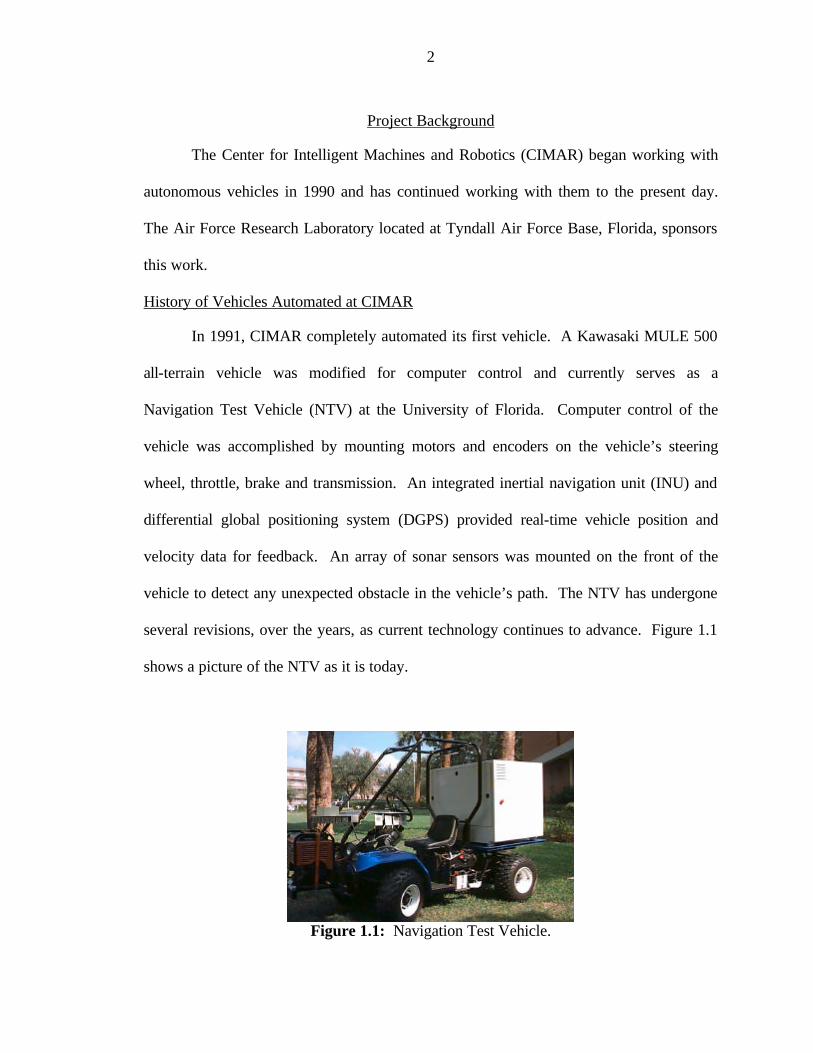
In 1991, CIMAR completely automated its first vehicle. A Kawasaki MULE 500
all-terrain vehicle was modified for computer control and currently serves as a
Navigation Test Vehicle (NTV) at the University of Florida. Computer control of the
vehicle was accomplished by mounting motors and encoders on the vehicle’s steering
wheel, throttle, brake and transmission. An integrated inertial navigation unit (INU) and
differential global positioning system (DGPS) provided real-time vehicle position and
velocity data for feedback. An array of sonar sensors was mounted on the front of the
vehicle to detect any unexpected obstacle in the vehicle’s path. The NTV has undergone
several revisions, over the years, as current technology continues to advance. Figure 1.1
shows a picture of the NTV as it is today.
Figure 1.1: Navigation Test Vehicle.
3
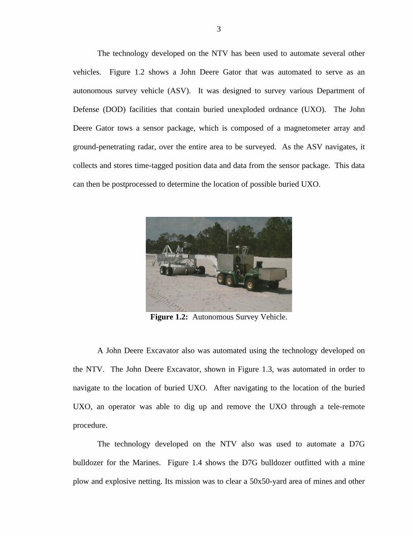
The technology developed on the NTV has been used to automate several other
vehicles. Figure 1.2 shows a John Deere Gator that was automated to serve as an
autonomous survey vehicle (ASV). It was designed to survey various Department of
Defense (DOD) facilities that contain buried unexploded ordnance (UXO). The John
Deere Gator tows a sensor package, which is composed of a magnetometer array and
ground-penetrating radar, over the entire area to be surveyed. As the ASV navigates, it
collects and stores time-tagged position data and data from the sensor package. This data
can then be postprocessed to determine the location of possible buried UXO.
Figure 1.2: Autonomous Survey Vehicle.
A John Deere Excavator also was automated using the technology developed on
the NTV. The John Deere Excavator, shown in Figure 1.3, was automated in order to
navigate to the location of buried UXO. After navigating to the location of the buried
UXO, an operator was able to dig up and remove the UXO through a tele-remote
procedure.
The technology developed on the NTV also was used to automate a D7G
bulldozer for the Marines. Figure 1.4 shows the D7G bulldozer outfitted with a mine
plow and explosive netting. Its mission was to clear a 50x50-yard area of mines and other

4
obstructions in order to create a landing area for the deployment of the Marines and their
supplies.
Figure 1.3: Autonomous John Deere Excavator.
Figure 1.4: Autonomous D7G Bulldozer.
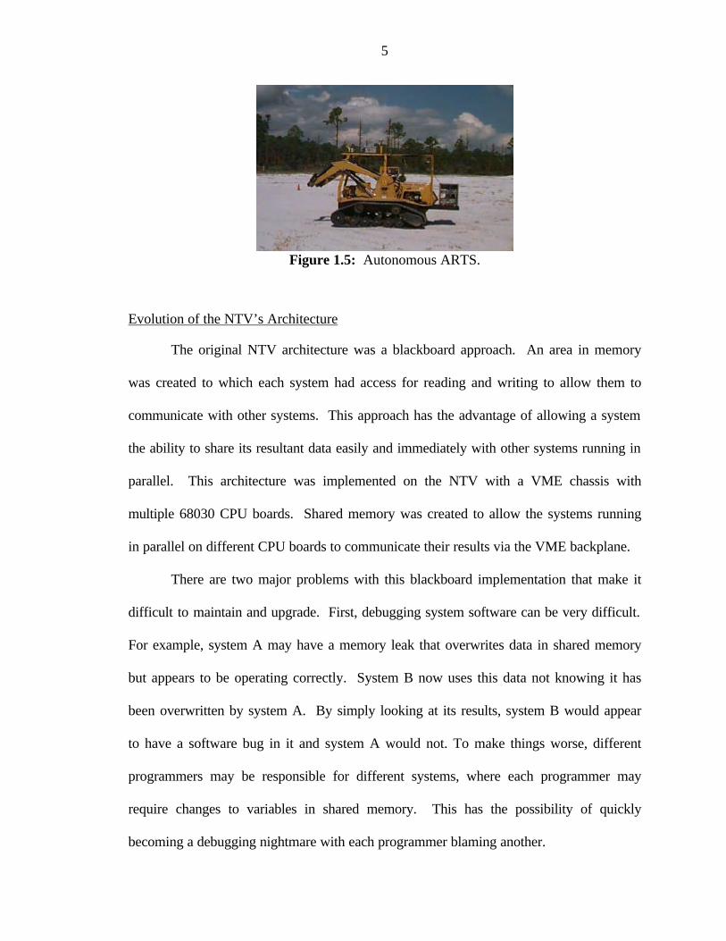
The latest vehicle to use the technology developed on the NTV is the All-Purpose
Remote Transport System (ARTS) shown in Figure 1.5. ARTS is a commercially
available vehicle outfitted with a tele-remote package developed by Applied Research
Associates, Inc. of Tyndall Air Force Base, FL. This vehicle was automated for a
demonstration during the October 1999 Joint Architecture for Unmanned Ground
Vehicles (JAUGS) working group meeting held at the University of Florida.
5
Figure 1.5: Autonomous ARTS.
Evolution of the NTV’s Architecture
The original NTV architecture was a blackboard approach. An area in memory
was created to which each system had access for reading and writing to allow them to
communicate with other systems. This approach has the advantage of allowing a system
the ability to share its resultant data easily and immediately with other systems running in
parallel. This architecture was implemented on the NTV with a VME chassis with
multiple 68030 CPU boards. Shared memory was created to allow the systems running
in parallel on different CPU boards to communicate their results via the VME backplane.
There are two major problems with this blackboard implementation that make it
difficult to maintain and upgrade. First, debugging system software can be very difficult.
For example, system A may have a memory leak that overwrites data in shared memory
but appears to be operating correctly. System B now uses this data not knowing it has
been overwritten by system A. By simply looking at its results, system B would appear
to have a software bug in it and system A would not. To make things worse, different
programmers may be responsible for different systems, where each programmer may
require changes to variables in shared memory. This has the possibility of quickly
becoming a debugging nightmare with each programmer blaming another.
6
A second problem with this blackboard implementation is the difficulty in
transferring only one system to another application or replacing an existing system with a
different one. Take for example a system that provides position feedback for the AGV.
Suppose the positioning system on AGV 1 was tested fully and known to operate
correctly. Now, it is desired to use this positioning system on a newly developed AGV 2.
In order for this transfer to work, both the hardware and software on AGV 2 must be
identical to AGV 1. That is, AGV 2 also must have a VME chassis and must have the
exact shared memory structure. Obviously this is not always the case, and substantial
hardware and software changes must be made in order to use the positioning system on
AGV 2.
Because of these problems a new architecture was designed. Based on experience
from previous work, one main requirement was specified for this new architecture. The
architecture must allow systems to be self-contained submodules, where only the
interface of each submodule is defined rigorously. The effect of this requirement benefits
both the developer and the user. The developer now has a great amount of freedom in
choosing specific hardware and software for his or her system. And, the user now has the
ability to scale his or her AGV’s functionality by combining different submodules.
Developing an architecture that meets this requirement is a two-step process
accomplished by first determining a list of submodules required to automate a vehicle
and then determining their interface. The Modular Architecture eXperimental (MAX),
currently being developed at the University of Florida, attempts to meet this requirement.
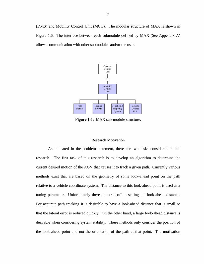
MAX currently consists of the following submodules: Position System (POS),
Vehicle Control Unit (VCU), Path Planner (PLN), Detection and Mapping System
7
(DMS) and Mobility Control Unit (MCU). The modular structure of MAX is shown in
Figure 1.6. The interface between each submodule defined by MAX (See Appendix A)
allows communication with other submodules and/or the user.
MobilityControl
Unit
OperatorControl
Unit
PathPlanner
PositionSystem
Detection &MappingSystem
VehicleControl
Unit
Figure 1.6: MAX sub-module structure.
Research Motivation
As indicated in the problem statement, there are two tasks considered in this
research. The first task of this research is to develop an algorithm to determine the
current desired motion of the AGV that causes it to track a given path. Currently various
methods exist that are based on the geometry of some look-ahead point on the path
relative to a vehicle coordinate system. The distance to this look-ahead point is used as a
tuning parameter. Unfortunately there is a tradeoff in setting the look-ahead distance.
For accurate path tracking it is desirable to have a look-ahead distance that is small so
that the lateral error is reduced quickly. On the other hand, a large look-ahead distance is
desirable when considering system stability. These methods only consider the position of
the look-ahead point and not the orientation of the path at that point. The motivation

8
behind this part of the research is to allow for smaller look-ahead distances without
giving up system stability.
The second task of this research is to develop a control algorithm that executes the
AGV’s desired motion. There are two main motivations for this work. The first
motivation is to have the ability to operate the NTV under various conditions and speeds.
Operating conditions most likely change as new applications are established for the
technology developed on the NTV. Some possible changes in operating conditions
include the weight of the payload, towing a trailer, the desired vehicle speed, and the type
of ground on which it is operating (i.e., asphalt, grass, sand, etc…). All of these
conditions affect the ability of the NTV to navigate a path accurately. Currently, if the
operating conditions are too different, the NTV must be re-tuned to achieve an acceptable
performance.
Using the MAX architecture, it is desired to develop an MCU that has the ability
to operate under these various conditions without the need to re-tune it. This suggests
that the MCU must have the ability to adapt to its current operating conditions.
The second motivation for this part of the research is to reduce the amount of time
required to transfer the technology to different vehicles. One of the main reasons for
developing a modular architecture is to have the ability of transferring a module from one
vehicle to another or to be able to use modules that are made up differently on the same
vehicle. This makes sense for a POS module since it is, for the most part, independent of
the vehicle it is on. For example, one positioning system could be made up of GPS and
INS units while another positioning system could be made up of just a GPS unit. Since

9
by using MAX the interfaces between the two positioning systems are the same, they can
easily be switched on the same vehicle or transferred to a new vehicle.
The ability to switch or transfer modules becomes much more difficult when
dealing with the MCU module. Without using MAX architecture, control of a ground
vehicle was accomplished typically by commanding a throttle position and steering wheel
angle for a car-like vehicle or commanding left track and right track velocities for a
tracked vehicle. Obviously the commands depended highly on the type of vehicle. By
using MAX, the commands to control the vehicle are now the same, a propulsive wrench
and a resistive wrench. Additionally, ground vehicles typically will use the same
components of the propulsive wrench and resistive wrench. The component Fx is used to
control the vehicle’s linear speed, and the component Mz is used to control the vehicle’s
angular speed.
Having the commands to control an AGV be the same for most ground vehicles
makes the idea of being able to switch out or transfer the MCU more feasible. Therefore,
the second motivation for this part of the research is to develop an MCU that can be
transferred to different vehicles with few or no changes to the MCU. This suggests that
the MCU must have the ability to adapt not only to different operating conditions but also
to different vehicles.
Research Objective
The objective of this research is to develop an adaptive control algorithm for the
NTV to track a given path accurately at speeds up to 4.5 meters per second. This task is
broken down into two subtasks. First, develop an algorithm to determine the current
10
desired motion of the AGV that causes it to track the given path. Second, develop an
adaptive control algorithm that executes the AGV’s desired motion.
The remainder of this dissertation is outlined as follows: Chapter 2 is a broad
overview of different AGVs and their navigation architectures. Chapter 3 introduces a
new path-tracking algorithm that gives the vehicle’s desired motion based on the current
vehicle position and orientation relative to a path. Chapter 4 presents a fuzzy model
reference learning controller (FMRLC) to track the AGV’s desired motion. Chapter 5
presents the development of a simulation of the NTV and presents the results of using the
simulation to test the new path-tracking algorithm and the adaptive control algorithm. It
also presents the test results from implementing the algorithms on the NTV. Chapter 5
concludes by presenting the test results from implementing the path-tracking algorithm
and adaptive control algorithm on a synchronous drive vehicle and a tracked vehicle.
And finally, Chapter 6 presents some conclusions and future work.
11
CHAPTER 2 REVIEW OF THE LITERATURE
Recently, within the past couple of decades, there has been much research in the
area of autonomous mobile robots. The reason for the sudden interest in autonomous
mobile robots is the advancement of supporting technology. Both sensor and computing
technology have increased greatly. Sensors are more accurate and give more information
about the current state of the robot and its environment. And computers are faster and
have larger memory to run larger, more complicated programs. The advancement of
these two areas has made possible the idea of autonomous mobile robots. Today,
autonomous mobile robots consist of air, land, and sea vehicles. This chapter focuses on
the research done on autonomous mobile land vehicles, or autonomous ground vehicles
(AGVs). First we consider some of the current applications of AGVs. Then we review
the current research on various navigation architectures.
Autonomous Ground Vehicle Applications
There are many applications for autonomous ground vehicles. The motivations
for automating different vehicles are typically to reduce risk of human life or injury in
hazardous areas, to relieve human operators from overly monotonous tasks, or to increase
the precision of navigation. Some of these applications are discussed below.
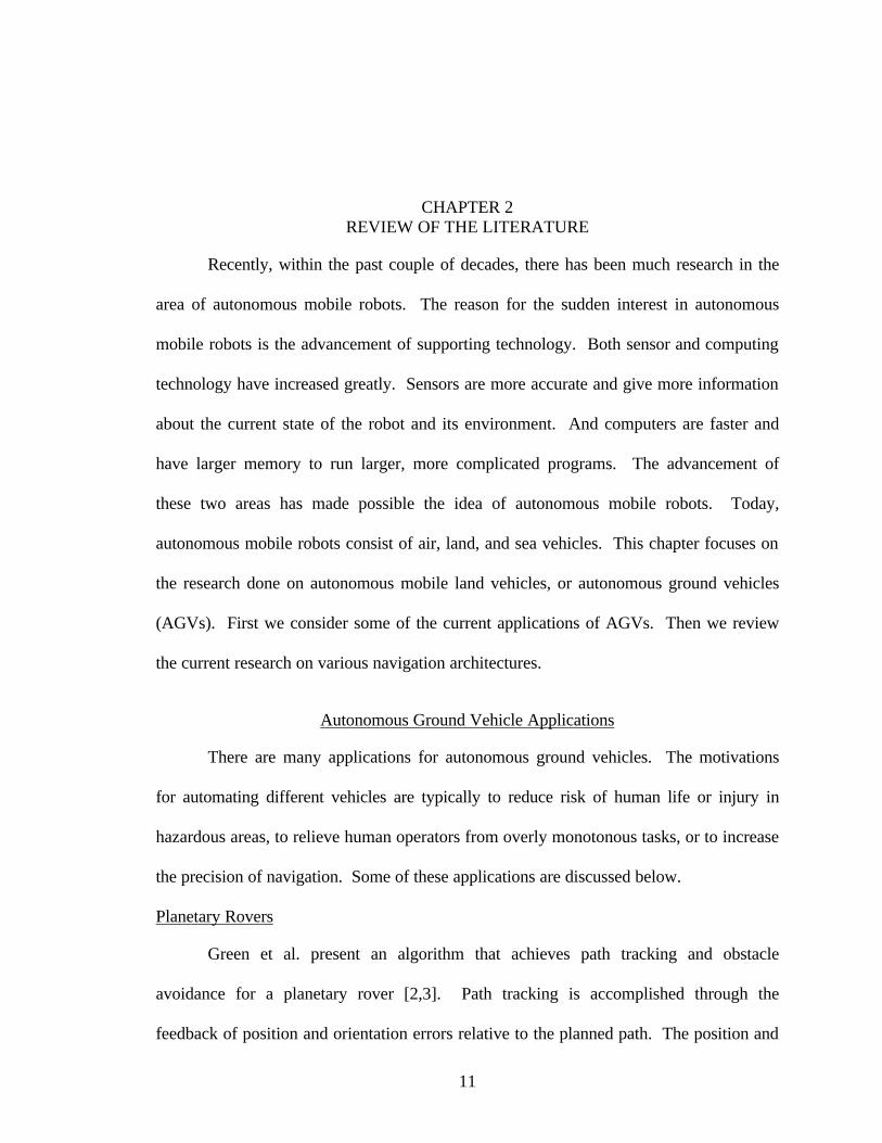
Planetary Rovers
Green et al. present an algorithm that achieves path tracking and obstacle
avoidance for a planetary rover [2,3]. Path tracking is accomplished through the
feedback of position and orientation errors relative to the planned path. The position and

12
orientation of the rover is estimated using an inertial navigation unit integrated with an
odometer. The rover avoids obstacles by creating an artificial potential field from the
data received from a range sensor. An obstacle avoidance error is calculated from this
artificial potential field. Both the tracking and the obstacle avoidance errors are used as
inputs to a linear-feedback steering controller. Simulated results of the controller are
presented.
Boissier presents the work done by the French Space Agency on planetary rovers
for the IARES Eureka project [4]. The IARES mobile robot has six independent
steerable wheels, three rotating axles, wheel and walking modes, passive adaptation to
obstacles along the transversal axis and mixed passive/active longitudinal deformation,
active wheel loading equalization on slopes and maximum speeds of 0.10 m/s or 0.35
m/s. It has a SAGEM inertial unit for localization that uses zero velocity updates to
minimize the amount of drift in position. The IARES mobile robot also has stereovision
in order to create a digital terrain model that is used to navigate the vehicle. It was
evaluated successfully in different terrain conditions for both predictive tele-remote
operation and autonomous navigation.
Agricultural Vehicles
O’Connor et al. at Stanford University rely solely on Carrier Phase Differential
GPS (CPGPS) to provide position and attitude feedback to control the position of
agricultural equipment relative to a preplanned path [5]. The position and attitude are
calculated using four single-phase GPS antennas on the vehicle. The test platform used
by O’Connor et al. to test autonomous navigation is a John Deere 7800 tractor. A hybrid
controller is used to control the vehicle’s heading. For large heading errors, a “bang-
bang” control technique is used. Otherwise, for small heading errors, a Linear Quadratic

13
Regulator is used. Tests showed the lateral position standard deviation to be less than 2.5
cm and the heading standard deviation to be less than 1 degree.
Another group interested in autonomous agriculture vehicles is from the Silsoe
Research Institute in Bedford, UK [6]. Marchant et al. present a row-following
autonomous vision-guided agriculture vehicle. They use image analysis and odometer
data to localize the vehicle. A proportional controller is used to track the desired path.
Marchant tested the vehicle on four fields of cauliflower. The control error for these runs
was determined to be less than 20 mm RMS.
Cleaning Vehicles
Hofner and Schmidt present MACROBE, an autonomous floor-cleaning and
inspecting robot [7,8]. Navigation is achieved by executing one of five preprogrammed
motion macros. A planner on MACROBE uses its current knowledge of the workspace
to generate a serpentine path made up of these motion macros. If an unexpected obstacle
is encountered, MACROBE adds it to its knowledge of the workspace and then plans a
new path.
Ulrich et al., from the Swiss Institute of Technology in Lausanne, Switzerland,
present an autonomous vacuum cleaner [9]. A Koala robot is used as the platform for the
autonomous vacuum cleaner. The robot is equipped with a 2-DOF arm that is used to
facilitate the cleaning process. The arm also is used tactically to sense unknown objects
and then classify them as legs, walls, corners or unknowns. Through the use of the object
data along with compass and odometer data, the robot builds a map of its workspace. An
algorithm to clean the workspace begins by attempting to travel the perimeter of the
workspace. This allows the robot to build an initial map of its workspace. After the
perimeter is traversed, the robot attempts to clean the interior part of the workspace by
14
traveling back and forth between known walls. Ulrich tested the robot in a 2-3 square
meter area that was covered with sawdust. The robot was able to clean 95% of the area
in its internal map.
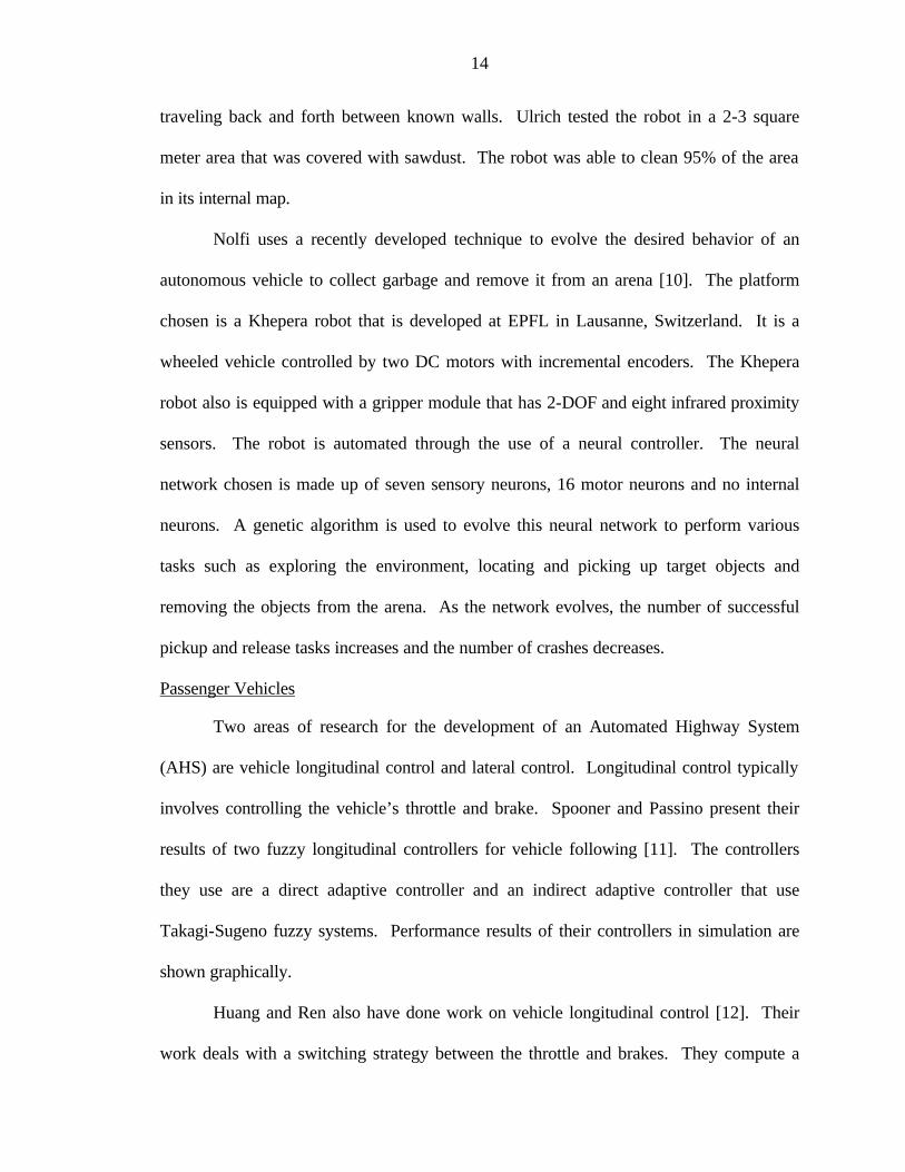
Nolfi uses a recently developed technique to evolve the desired behavior of an
autonomous vehicle to collect garbage and remove it from an arena [10]. The platform
chosen is a Khepera robot that is developed at EPFL in Lausanne, Switzerland. It is a
wheeled vehicle controlled by two DC motors with incremental encoders. The Khepera
robot also is equipped with a gripper module that has 2-DOF and eight infrared proximity
sensors. The robot is automated through the use of a neural controller. The neural
network chosen is made up of seven sensory neurons, 16 motor neurons and no internal
neurons. A genetic algorithm is used to evolve this neural network to perform various
tasks such as exploring the environment, locating and picking up target objects and
removing the objects from the arena. As the network evolves, the number of successful
pickup and release tasks increases and the number of crashes decreases.
Passenger Vehicles
Two areas of research for the development of an Automated Highway System
(AHS) are vehicle longitudinal control and lateral control. Longitudinal control typically
involves controlling the vehicle’s throttle and brake. Spooner and Passino present their
results of two fuzzy longitudinal controllers for vehicle following [11]. The controllers
they use are a direct adaptive controller and an indirect adaptive controller that use
Takagi-Sugeno fuzzy systems. Performance results of their controllers in simulation are
shown graphically.
Huang and Ren also have done work on vehicle longitudinal control [12]. Their
work deals with a switching strategy between the throttle and brakes. They compute a

15
control signal for the throttle and a control signal for the brake. Each signal is optimized
in order to meet some tracking criterion by a learning algorithm. These two signals then
are used to determine brake and throttle positions. Results from simulations are
presented graphically.
Vehicle lateral control, on the other hand, involves controlling the vehicle’s
steering. Unyelioglu et al. present their design and stability analysis of a controller for
lane following [13]. Their objective is to steer a vehicle so that it stays in the middle of
the lane. This is accomplished by defining a reference line in the middle of the lane and a
look-ahead point on the vehicle’s longitudinal axis at a given distance in front of the
vehicle. The controller uses the offset distance between the look-ahead point and the
point on the reference line closest to the look-ahead point. Using Routh-Hurwitz stability
criterion they prove that for a given range of speeds, by choosing a sufficiently large
look-ahead distance, the system is stable for that range. Simulation results are given to
demonstrate the performance of their controller.
O’Brien et al. also address the lateral motion control of automated highway
vehicles [14]. They designed an H∞ controller to track the center of the current lane on
both curved and straight highways. The result of considering performance requirements
in the controller design, is a controller that is robust to model uncertainty. The
controller’s robustness to different speeds, road conditions and wind gusts are examined.
The controller is tested in simulation for various conditions. For each condition tested,
the lateral offset is less than 20 centimeters and the yaw angle error is less than 0.01
radians.
Two other areas of research dealing with passenger vehicles are active steering
assistance and parallel parking. The concept behind active steering assistance is to
16
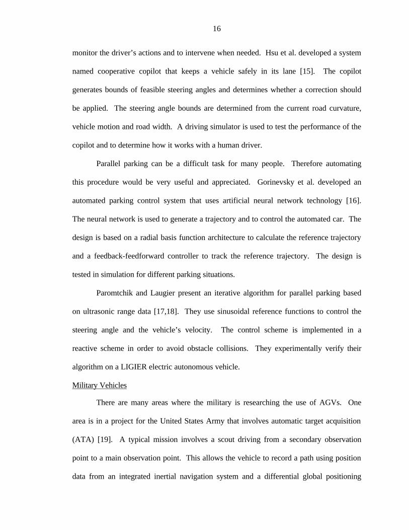
monitor the driver’s actions and to intervene when needed. Hsu et al. developed a system
named cooperative copilot that keeps a vehicle safely in its lane [15]. The copilot
generates bounds of feasible steering angles and determines whether a correction should
be applied. The steering angle bounds are determined from the current road curvature,
vehicle motion and road width. A driving simulator is used to test the performance of the
copilot and to determine how it works with a human driver.
Parallel parking can be a difficult task for many people. Therefore automating
this procedure would be very useful and appreciated. Gorinevsky et al. developed an
automated parking control system that uses artificial neural network technology [16].
The neural network is used to generate a trajectory and to control the automated car. The
design is based on a radial basis function architecture to calculate the reference trajectory
and a feedback-feedforward controller to track the reference trajectory. The design is
tested in simulation for different parking situations.
Paromtchik and Laugier present an iterative algorithm for parallel parking based
on ultrasonic range data [17,18]. They use sinusoidal reference functions to control the
steering angle and the vehicle’s velocity. The control scheme is implemented in a
reactive scheme in order to avoid obstacle collisions. They experimentally verify their
algorithm on a LIGIER electric autonomous vehicle.
Military Vehicles
There are many areas where the military is researching the use of AGVs. One
area is in a project for the United States Army that involves automatic target acquisition
(ATA) [19]. A typical mission involves a scout driving from a secondary observation
point to a main observation point. This allows the vehicle to record a path using position
data from an integrated inertial navigation system and a differential global positioning
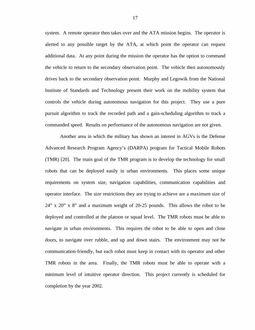
17
system. A remote operator then takes over and the ATA mission begins. The operator is
alerted to any possible target by the ATA, at which point the operator can request
additional data. At any point during the mission the operator has the option to command
the vehicle to return to the secondary observation point. The vehicle then autonomously
drives back to the secondary observation point. Murphy and Legowik from the National
Institute of Standards and Technology present their work on the mobility system that
controls the vehicle during autonomous navigation for this project. They use a pure
pursuit algorithm to track the recorded path and a gain-scheduling algorithm to track a
commanded speed. Results on performance of the autonomous navigation are not given.
Another area in which the military has shown an interest in AGVs is the Defense
Advanced Research Program Agency’s (DARPA) program for Tactical Mobile Robots
(TMR) [20]. The main goal of the TMR program is to develop the technology for small
robots that can be deployed easily in urban environments. This places some unique
requirements on system size, navigation capabilities, communication capabilities and
operator interface. The size restrictions they are trying to achieve are a maximum size of
24” x 20” x 8” and a maximum weight of 20-25 pounds. This allows the robot to be
deployed and controlled at the platoon or squad level. The TMR robots must be able to
navigate in urban environments. This requires the robot to be able to open and close
doors, to navigate over rubble, and up and down stairs. The environment may not be
communication-friendly, but each robot must keep in contact with its operator and other
TMR robots in the area. Finally, the TMR robots must be able to operate with a
minimum level of intuitive operator direction. This project currently is scheduled for
completion by the year 2002.
18
Security Vehicles
There are many applications for both indoor and outdoor security AGVs.
ROBART III is an indoors-nonlethal autonomous security response robot presented by
Ciccimaro et al. [21]. It is designed to operate in a previously unexplored area with little
support required from the operator. It is capable of detecting intruders through the use of
eight passive-infrared motion detectors. The infrared motion detectors are validated
partially by a Doppler microwave motion detector. A black-and-white video surveillance
camera mounted to the robot’s head is used for further assessment of possible intruders.
The nonlethal response capabilities include a Gatling gun and three sirens. The Gatling
gun is a six-barreled pneumatically powered gun capable of firing tranquilizer darts. A
visible laser is used to facilitate the accuracy of the gun when it is operated remotely.
The three sirens are capable of an ear-piercing 103 decibels that can alert those nearby
and disorient the intruder.
Pastore et al. present their work on the Mobile Detection Assessment and
Response System-Exterior (MDARS-E), an outdoor security AGV [22]. Robotics
Systems Technology developed the MDARS-E. Navigation is accomplished by
combined inputs from differential GPS, a fiber-optic gyro, a wheel odometer, and
landmark recognition. Obstacle avoidance is achieved with a two-tier layered approach.
Long-range sensors are used to provide first-alert obstacle detection from 0 to 100 feet.
Short-range sensors are used to provide higher resolution data for precise obstacle
avoidance. The sensors that are used for obstacle detection include radar, laser ranging,
ultrasonic ranging, and stereovision. Two sensors are used for intruder detection, vision
and radar, to achieve a high probability of detection and to minimize false detections.

19
Inspection Vehicles
AIRIS 21 is an underwater inspection robot presented by Koji [23]. The specific
task for the AIRIS 21 robot is to inspect the outside surface of a reactor pressure vessel of
nuclear power stations. It performs a nondestructive inspection of welds in the reactor
pressure vessel shell from the inside. The AIRIS 21 uses thrusters to provide a chamber
underneath it with negative pressure. This allows it to be sucked securely onto the
reactor pressure vessel’s wall. Two drive wheels and one idle wheel enable it to
maneuver on the wall. Position of the robot is accomplished with a depth gauge, an
optical beam, gravity sensor and an encoder. The depth gauge is used to determine the
elevation of the robot. The optical beam is used to locate a known structure relative to
the robot. Then, a map of the operating environment is used to locate the robot. The
gravity sensor is used to determine the direction of travel while the encoder keeps track
of the distance traveled.
A wheeled, multi-articulated robot that operates in a sewage system is presented
by Cordes et al. [24]. The objective behind this project is to be able to inspect Germany’s
360,000-km long public sewage system. Germany’s public sewage system is over 25
years old and possibly could be polluting the soil and ground water. The robot is
required to operate wirelessly, to navigate 90-degree turns and steps of 0.3 meters high,
and to operate in pipes with a diameter of 20 to 80 centimeters. The design looks like a
wheeled snake that consists of different modules. These modules include sensor, drive,
and power supply modules. This allows the driving and the sensing modules to be
developed independently.

20
Autonomous Ground Vehicle Navigation Architecture
In general, current navigation architectures are labeled as behavioral, hierarchical
or a hybrid of behavioral and hierarchical. Behavioral architectures, also known as
reactive architectures, assign the AGV to execute a particular behavior because of current
sensor readings. The behaviors are defined in such a way that they cause the AGV to
tend toward completing its task. This allows the vehicle to navigate reliably with quick
response in a dynamic environment. However, as the complexity of the AGV’s task or
its operating environment increases, the number of behaviors usually increases as well.
This makes it very difficult to predict the behavior of the AGV, and it makes it more
difficult for the designer to determine the correct behavior for all possible sensor
readings. Also, behavioral architectures do not guarantee the best solution since they
consider only the current sensor readings.
Hierarchical, or top-down, architectures break down the AGV’s task into subtasks
and create functions to achieve these subtasks. This allows for the design of a
straightforward approach to accomplishing the task. Hierarchical architectures typically
maintain a model of its operating environment. They use this model along with
sophisticated planners to determine the best course of action in order to achieve a task.
Unfortunately, using sophisticated planners also tends to be complex, and results in a
slow response to changing environments.
Hybrid architectures attempt to combine behavioral and hierarchical architectures
in order to attain the desirable qualities of both architectures while overcoming their
individual shortcomings.
21
Behavioral Architecture
Some of the recent methods used to implement behavioral architecture include
potential field [25], fuzzy logic [26-32], neural networks [33-35] and genetic algorithms
[36,37]. Some researchers have combined one or more of these methods in an attempt to
overcome the weaknesses of a particular method with the strengths of another. Some of
these combinations are fuzzy-neural networks [38-42], fuzzy-genetic algorithms [43],
fuzzy potential field [44,45] and fuzzy-neural networks-genetic algorithms [46].
Song and Sheen present a fuzzy-neural controller for obstacle avoidance of a
differentially driven vehicle [40]. The operating environment is assumed to be unknown
completely and, the vehicle is required to maneuver to a target location. Heuristic rules
are combined with a neural network to map input from sonar sensors to the left and right
motor velocities. Two behaviors implemented for vehicle navigation include avoid
obstacle and danger. The avoid obstacle behavior attempts to navigate the vehicle in the
direction of the target unless impeded by an obstacle. The danger behavior is used to
escape from any undesirable situations. When the danger behavior is activated, the
vehicle spins around to find a direction of escape. The danger behavior takes priority
over the avoid obstacle behavior. Results are shown graphically of a robot navigating to
a target while avoiding walls and a box-shaped obstacle.
A sensory-based navigation scheme is presented by Tani and Fukumura [35]. The
navigation architecture consists of two levels, a control level and a navigation level. The
control level incorporates a potential method in order to limit the desired trajectories so
that each one is smooth and avoids obstacles. This leaves the task of the navigation level
to decide the direction of travel at branches in the task space. A recurrent neural network

22
is used to accomplish this task. The network is trained through the supervision of a
trainer who knows the optimal path.
The mobile robot YAMABICO is used to test this navigation technique. The
experiment involves navigating the task space by alternating between a figure 8 route and
a figure 0 route. At a specific branch in the task space, the vehicle must switch between
the two different routes by deciding the direction of travel. Results of this test are shown
graphically where for the most part, the navigation level chose the correct direction of
travel at the various branches in the task space.
Hoffman and Pfister present a fuzzy logic controller to navigate a vehicle to a
goal point while avoiding obstacles [43]. The fuzzy logic controller is used to map the
perceived input to an appropriate control action. This fuzzy logic controller is designed
automatically through the use of a genetic algorithm. The genetic algorithm uses an
objective function to select the best individuals for reproduction of offspring. The fuzzy
logic controller’s performance is measured with respect to the two tasks of reaching the
goal and avoiding obstacles. If the vehicle collides with an obstacle the controller is
given a reward proportional to the number of steps prior to the collision. If the vehicle
does not collide but does not reach the goal in the allotted steps, an additional reward is
given depending on how close the vehicle is to the goal. If the vehicle is within a given
distance to the goal, the controller receives a third reward. The method was applied
successfully and the results are shown graphically.
Hierarchical Architecture
Hierarchical architectures typically involve either a path-tracking or trajectory-
tracking algorithm. Since the work done here involves path tracking, a more detailed
review of hierarchical architectures is warranted. Desired paths or trajectories can be
23
generated in real-time based on current sensor readings or generated once based on a map
of the operating environment. The method used, either real-time or not, to generate the
paths or trajectories generally depends on whether the operating environment is known a
priori and if it is static. Once the path or trajectory is known, there are several different
techniques used to track the path or trajectory. Some of these techniques include
Proportional-Integral-Derivative (PID) [47-53], pure pursuit [54-56], sliding-mode
[57,58], state feedback [59-66], fuzzy logic [67,68], neural networks [69-73] and fuzzy
neural networks [74,75].
PID techniques calculate errors based on the path or trajectory and the current
vehicle pose and velocity. These errors, and possibly their derivative and integral, are
multiplied by gains to determine the controlled input to the system. The first method
used to control the NTV, called follow-the-carrot, is a PID technique. The follow-the-
carrot path tracking method comes from the idea of holding a carrot in front of a farm
animal in order to coax the animal to move in a desired direction. With this in mind, the
follow-the-carrot method calculates a desired heading from the current vehicle position to
a look-ahead point called the carrot. The look-ahead point is a point on the path that is a
given distance in front of the orthogonal projection of the current vehicle position onto
the path. A PID controller is used with the error between the vehicle’s current heading
and desired heading as its input and outputs the current steering wheel angle. This
method works well for straight paths but has problems with curved paths. By having the
look-ahead point a certain distance in front of the vehicle on the path, the desired heading
causes the vehicle to cut corners. Even if the vehicle were able to track the desired
heading with no errors, the vehicle would still have errors in its position.
24
Kanayama and Fahroo propose a new steering function as a line tracking method
for nonholonomic vehicles [51]. The current state of a ground vehicle can be represented
by its current linear speed, v, and its current path curvature, κ = 1/r. Therefore, their
controller is designed to determine the optimal change in path curvature in order to track
a given line. They choose to control the vehicle’s path curvature because it is related
more directly to vehicle control, and it is independent of the global coordinate system.
The steering function they propose is:
( ) dcbads
d∆−−−−= 1θθκ
κ,
where a, b and c are positive constants, κ is the current vehicle’s path curvature, θ-θ1 is
the vehicle’s heading error and ∆d is the vehicle’s position error. Immediately, it is
apparent that there is a problem of mixed units in their proposed steering function.
Unfortunately, Kanayama and Fahroo did not address this issue. By requiring that the
magnitude of (θ-θ1) be less than π/2, they determined that the relationship between the
constants should be, a = 3k, b = k2 and c = k3, for the controller to be stable. The term k is
the gain of the steering function and controls how fast or how slow the vehicle converges
to the line. This technique was tested in simulation as well as on the autonomous vehicle
Yamabico. The results of these tests are shown graphically for different values of the
steering function gain k.
Egerstedt et al. present the autonomous navigation of a car-like robot by tracking
a reference point [49]. As long as the vehicle’s position and heading errors relative to the
reference point are small, the reference point moves along the path as the vehicle follows
it. If the errors are too large, the reference point may stop to wait for the vehicle.
Therefore, they call the reference point a virtual vehicle. The location of the virtual
(2.1)
25
vehicle depends on both the vehicle’s current speed and position. Once the location of
the virtual vehicle is determined, the steering is controlled by the proportional controller:
( )df k ϕϕδ −−= ,
where δf is the steering angle, ϕ is the vehicle heading, ϕd is the desired heading and k is
chosen based on the vehicle’s maximum steering angle. This technique was tested on a
modified radio-controlled car and a Nomad 200. Results for both vehicles are shown
graphically and considered satisfactory.
A geometric path-tracking control of a differential drive vehicle that takes into
account the kinematic and dynamic properties of the vehicle is proposed by DeSanits
[48]. The vehicle has rear differentially driven wheels and a front castor wheel. A
reference frame is placed at the center of the rear wheel’s axle. Using this reference
frame, differential equations of the vehicle’s dynamic model are derived. Then, this
model is simplified by assuming no slip in either the lateral or longitudinal directions. A
path is assumed to be defined by a set of continuous functions of position and orientation
that the guide point must track. It is assumed also that both velocity and acceleration
profiles of the path are given and described by continuous functions. A path-tracking
controller is designed then in terms of the heading, lateral, and velocity errors. Assuming
the errors are kept sufficiently small, the vehicle’s controller can be decentralized
allowing separate controllers for speed and steering. It turns out that the speed controller
is in the form of a PI controller and the steering controller is in the form of a PID
controller. Therefore, the gains of the controllers are determined through the use of
classical PID techniques. An example of applying this control technique to a wheelchair
is given, but no results are given of its accuracy.
(2.2)

26
Lee and Williams present a control method for a differentially driven autonomous
mobile robot [52]. The control structure is made up of two loops. In the vehicle
controller loop, a trajectory generator first provides the desired displacement and rate.
Then, the errors between the desired and actual are used as input to a PID controller that
converts them to a desired torque. The second loop calculates an error between a desired
posture and an actual posture. The desired posture is determined using the desired
displacement and rate along with a kinematic model of the vehicle. Similarly, the actual
posture is determined with the measured displacement and rate along with a kinematic
model of the vehicle. The error in posture is used then to calculate a torque in order to
drive the error to zero. The total commanded torque is the sum of the torque calculated
from the vehicle controller and the torque computed from the error in posture.
This navigation technique was tested both in simulation and experimentally.
Experimental results are shown graphically of the controller’s ability to handle an initial
lateral error of 1 cm, initial longitudinal errors of 0.5, 1 and 2 cm, and initial heading
errors of 1, 2 and 3 degrees. The lateral error converged almost to zero in approximately
six seconds. The longitudinal and heading errors were able to converge to zero in about
0.2 seconds.
Choi presents an adaptive controller for the lateral position of a vehicle for the
Intelligent Vehicle Highway System (IVHS) [47]. The lateral error is measured using
look-down sensing which can be realized using electrified wires, radar reflection or
buried permanent magnets. Using the lateral error as input, a PD type controller is
presented. This results in the possibility of a steady state error. In order to deal with this,
the PD controller is modified by adding an unknown lateral disturbance force. This
lateral force is used to model unmeasured disturbances such as wheel misalignment,

27
unbalanced tire pressure, side wind, and offset errors on the steering actuator or its
sensor. This unknown lateral force is updated continually based on Lyapunov criterion.
The controller was tested on a track that is 330 meters long and 5 meters wide.
Permanent magnets, 2.2 cm in diameter and 10.2 cm long, were placed every meter. At a
low speed of 10 m/s, the vehicle followed the center of the track with a maximum lateral
error of 0.1 meters. The controller was tested also at a higher speed of 22 m/s and again
the maximum lateral error was 0.1 meters.
A control technique for high-speed autonomous navigation of a full-size outdoor
vehicle is presented by Shin et al. [53]. This technique separates the control of the
vehicle speed and steering by choosing the center of the rear axle as the point on the
vehicle to control. The desired speed of the vehicle is determined by factors such as the
current path curvature and the vehicle’s distance to nearby obstacles. To control the
vehicle’s steering, a feedforward module that incorporates the vehicle’s dynamics is used
in conjunction with a feedback controller. The control input then takes the form:
iii KeRU += ,
where Ri is the feedforward compensation and Kei is the feedback error multiplied by
some gain.
The dynamic model of the feedforward compensator considers only the latency of
the steering. The latency is considered the dominant characteristic of the vehicle’s
dynamics. It is modeled using a lumped system of first-order lag. The feedforward
compensator, in effect, sends commands in advance so that the steering maneuver starts
before a turn is encountered.
The feedback controller uses the vehicle’s position, heading, and curvature errors.
Using the geometry of the errors, a quintic polynomial function is determined that
(2.3)
28
converges to zero at a specified look-ahead distance. Then, the variation of the steering
angle is determined from this polynomial. The look-ahead distance is used to adjust the
sensitivity of the system and is a function of the current vehicle speed.
Testing of this autonomous navigation technique was accomplished in simulation
and through experiments. In simulation, the technique was tested using an open-loop
controller, just the feedback controller, just the feedforward controller, and finally with
both the feedback and feedforward controller. The best results were obtained using the
feedback with the feedforward controller. The results of this technique had a position
error of 0.1 meters with a standard deviation of 0.1 meters, and a velocity error of 2.8
meters per second with a standard deviation of 4.8 meters per second.
Shin et al. used the autonomous vehicle Navlab as a test bed. The desired path
consisted of a 20-meter straight line ending with a 5-meter lateral jump and then followed
by an additional 80-meter straight line. Results are shown graphically for various
feedforward compensation times. With these results the feedforward compensation time
of Navlab is determined to be 0.5 seconds. Using this time, the navigation technique is
tested on a path that is over 500 meters in length at speeds up to 10 meters per second.
Results of this test are shown graphically and are considered acceptable.
Jagannathan et al. present the path planning and control of a nonholonomic
vehicle [50]. A path planner that considers the nonholonomic constraints generates a
desired trajectory. The control structure consists of an inner feedback linearizing loop to
eliminate the nonlinearities in their equation to model the vehicle dynamics. A second
feedback linearization loop is required after converting the path trajectories to a local
vehicle coordinate system. Finally, Lyapunov techniques are used to design an outer

29
control loop to guarantee that the vehicle follows the desired trajectory. This selection of
the control law yields a PD controller.
The path planning and control proposed by Jagannathan et al. is tested in
simulation. The width of the vehicle is assumed to be 10 cm and the radius of its wheels
is assumed to be 3 cm. The position and velocity gains for the outer loop PD controller
are set to 100 and 20, respectively, for a critically damped system. Several tests are done
where an initial position and orientation are specified, as well as a goal position and
orientation. Results of these tests are shown graphically.
Murphy presents a simple vehicle and path following model for vehicle
navigation at highway speeds [55]. A military HMMWV was modified by attaching
motors to the steering wheel, brake, and throttle. In addition, a video camera was
mounted on the vehicle in order to determine its lateral position on the road. Pure pursuit
is used to determine the instantaneous curvature of the vehicle’s path. Using the models
developed, it is proven that the system’s stability increases by reducing the controller
delay and decreases by increasing the vehicle speed. In order to compensate for the
computational delay of the vision, Murphy suggests using an inertial navigation sensor.
Ollero and Heredia present their stability analysis of a pure pursuit path tracking
technique that is applied to a computer controlled HMMWV [56]. Kinematic equations
of the vehicle’s motion are determined in terms of the vehicle’s speed and angular
velocity. The vehicle’s angular velocity is modeled by a first order differential equation.
The vehicle’s desired turning radius is calculated using pure pursuit:
x
LR
2
2
= , (2.4)
30
where L is the look-ahead distance and x is the lateral error. This is a proportional
controller where the look-ahead distance determines the gain to be applied to the lateral
error. Assuming a small lateral error and a small angle between the vehicle heading and
the heading from the vehicle position to the look-ahead position, they derive the
condition for stability to be L≥1.
Next, the stability is analyzed by assuming a time delay, τ, of the steering
command due to computing and communication delays. Conditions for stability are
derived and shown graphically by plotting the nondimensional quantities τ/T by L/(VT),
where T is the steering time constant and V is the vehicle velocity.
To determine the accuracy of their stability analysis, experimental data is taken of
the computer controlled HMMWV at speeds of 3, 6 and 9 meters per second. For each
speed, the minimum and maximum look-ahead distance that results in a stable system is
determined. The results are displayed graphically by plotting the stable look-ahead
distance determined by the analysis without delay and with delay as a function of velocity
and plotting the experimental results on the same plot. The experimental results require a
slightly larger look-ahead distance than the stability analysis with delay requires. This is
accounted for because of the fact that nonlinear terms are not considered in the vehicle
model.
Ku and Tsai present an autonomous navigation of an indoor vehicle that follows a
person [54]. The navigation technique presented is broken down into seven steps. First,
acquire an image. An image of the environment in front of the vehicle is captured using a
CCD camera that is mounted on the vehicle. In order to reduce the time to detect the
person to follow, a rectangular shape is attached to their back. The second step involves
detecting feature points of this rectangular shape. Third, transform the feature points

31
from the image coordinate system to a 3-dimensional space coordinate system and
determine the location of the person. Fourth, using a sequential pattern recognition
technique, determine if the person is walking straight or turning. Step five calculates the
speed of the person from the location of the person in consecutive cycles. Step six
calculates a desired turning radius of the vehicle using pure pursuit. Finally, step seven
controls the speed of the vehicle using a fuzzy control technique. This method is tested
using an autonomous vehicle and results are shown graphically. Successful and smooth
navigation is claimed while a person walks in different directions.
Balluchi et al. present a path-tracking controller designed according to sliding-
mode techniques for Dubin’s cars, i.e., cars that can only move forward with curvature
bounds [57]. They assume the forward velocity is given, and therefore consider only the
lateral stabilization of the vehicle to the desired path. The input of their controller
consists of the lateral and heading errors, the sign of the path curvature and the current
vehicle speed. Note that only the sign of the path’s curvature is used and not its
magnitude. This is a result of assuming that the path shape is not known a priori. Using
the sliding-mode design technique an equivalent control is derived. This result did not
satisfy the minimum turning radius constraint of their Dubin’s car. A control law similar
in form of the equivalent control is proposed instead. This control law converges to the
reference path while satisfying the constraints provided the initial position and heading
errors are small. This technique is tested in simulation and the results are shown
graphically.
State feedback techniques generally use kinematic equations to model the
vehicle’s motion. Then, these equations are converted and possibly linearized, to state
32
space equations. Using various methods, a feedback gain matrix is determined to control
the system.
Aguilar et al. present a path-following controller for differential drive mobile
robots [59]. It is assumed that a path exists whose curvature is both continuous and
bounded. A moving reference frame is defined with the origin located at the orthogonal
projection of the vehicle’s position onto the reference path and orientated with the
tangential of the path at that point in the direction to follow. Differential equations of the
position and heading errors are derived based on the location of the vehicle’s reference
frame relative to the moving reference frame. Using these differential equations and
assuming a nonzero linear velocity, a state feedback controller is presented to control the
vehicle’s angular velocity that drives the position and heading errors to zero.
Two constraints on the system are required for guaranteeing exponential stability.
The first constraint requires the distance from the vehicle to the path be less than the
current reference path curvature. This is required in order to be able to define the
reference frame uniquely. A second constraint is a result of dealing with discontinuities
with the path curvature. This constraint limits the distance the vehicle can be from the
path as a function of the current velocity.
The control laws are implemented on a robot of the Hilare family. The robot’s
position and orientation are determined by integrating the variation of each wheel. Two
different paths made up of line segments and arcs are used to test the controller. Results
of these two tests are presented graphically.
Hemami et al. present their work on the path tracking control of a mobile robot
with front steering [62]. Only the kinematic equations of the system are considered as the
vehicle is intended to operate at low speeds. The equations derived are based on a
33
coordinate system at the center of mass. With these equations, a state feedback controller
is designed to minimize the control input as well as the position and heading errors. The
performance index used to accomplish this is:
( )∫∞
++=0
222
21 tan dtrqqJ d δεε θ ,
where εd is the position error, εθ is the heading error, δ is the steering angle and q1, q2,
and r are weighting factors. The state feedback gain matrix is derived as functions of
known variables and of the weighting factors. Examples are presented that calculate the
state feedback gain matrix at different forward velocities. No results of its accuracy to
track paths are given from real experimental data or simulation.
Guldner et al. present a controller for the automatic steering of passenger cars
[63]. Some of the performance requirements of their design include being robust with
changing road adhesion due to different weather conditions, limiting the lateral
displacement to 0.15 meters with good road adhesion and 0.3 meters with poor road
adhesion, and keeping the passenger comfort similar to a manually steered vehicle. Their
control design considers a lookdown reference system where sensors to measure the
lateral offsets of the vehicle are placed on the front and rear bumpers. Dynamic
equations are derived in terms of the front and rear lateral displacements and their
derivatives. In order to deal with the performance requirements, the parameter space
approach in an invariance plane is used to determine a state feedback controller.
The controller is tested on a Pontiac 6000 STE Sedan. A 2-kilometer test track is
made up of straight sections as well as left and right turns with a turning radius of 800
meters. Magnets are placed every 1.2 meters over the entire track. The vehicle has a
gyroscope and accelerometer to record the motion of the vehicle, as well as
(2.5)
34
magnetometers on the front and rear bumpers. Results of the experiments are shown
graphically where the steady state error in the curves is approximately 0.2 meters for
good road adhesion and approximately 0.5 meters for poor road adhesion.
Behringer and MŸller present an autonomous vehicle based on vision that is able
to navigate on public roads in normal traffic [61]. One of the requirements of this vehicle
is to be able to recognize intersections and then to navigate the vehicle in the right
direction. In addition to the vision, a dead-reckoning system, made up of an odometer
and gyros, is used to measure the current state of the vehicle. Separate feedback
controllers are used to control the vehicle’s lateral and longitudinal movements. The
longitudinal controller is based on lookup tables to actuate the vehicle’s brake and
throttle. The lateral controller uses state feedback where the states are defined to be the
lateral offset, yaw angle rate, yaw angle, slip angle, and steering angle.
The autonomous navigation is tested on a track that includes curves of constant
radii of 40, 50 and 100 meters, as well as curves with approximately clothoid shape. The
results of these tests are shown graphically. The steering algorithm is claimed to be
sufficiently reliable such that the operation on arbitrary intersections is assumed to work
as well.
The tracking control of a mobile robot, using a time-varying state feedback
controller based on the backstepping technique, is presented by Jiang and Nijmeijer [64].
Local and global controllers are presented based on a kinematic model of the vehicle. In
addition, another controller is presented based on a simplified dynamic model.
Simulations in MATLAB were carried out to test the local and global controllers. The
results of their simulation showed that the local controller performs better for small initial
35
tracking errors and that the global controller was able to handle large initial tracking
errors.
Astolfi presents a controller for chained systems with two control inputs using a
discontinuous state feedback control law and applies it to a drive car-like vehicle [60].
The kinematic model of the car is given by
2
1
1
1
tan1sin
cos
v
vl
vy
vx
=
=
==
φ
φθ
θθ
&
&
&
&
,
where x and y are the location of the vehicle with heading θ, φ is the steering wheel angle,
and v1 and v2 are the vehicle velocity and steering wheel, respectively. This system is put
into a chained form using the state transformation:
yx
xl
x
xx
==
=
=
4
3
22
1
tan
tansec1
θ
φθ,
and input change:
+−=
232
12
1
2
1
coscossectansin3
cos
ulul
u
v
v
θφθθφ
θ .
Results of this controller, which was tested in simulation with different initial conditions,
are presented graphically.
Mouri and Furusho compare the results of using a PD controller versus using a
state feedback controller that was developed using linear quadratic (LQ) control for
navigating a vehicle on a highway [65]. The PD controller uses the lateral error to
(2.6)
(2.7)
(2.8)

36
determine a steering command. The proportional gain can be increased to achieve the
desired response and still converge by setting the derivative gain up to a certain point.
After that point, continuing to increase the proportional gain results in not being able to
construct a controller that provides both good response and convergence. Because of this
fact, a state feedback controller is developed using LQ control, where the lateral velocity
and the lateral deviation are chosen as states.
These two methods were tested on a vehicle with a speed of 80 km/h. The lateral
offset was determined from a magnetic sensor on the front bumper of the car that was
able to detect magnetic markers buried in the road. The PD control had large overshoots
when attempting to improve the systems time response. The system was also more
susceptible to noise. The gains for the LQ control could be increased by a factor of 10
compared to the PD controller gains that gave them the desired response and still
achieved the desired lateral convergence.
Rekow et al. present an adaptive steering controller for tractors using a
differential global positioning system [66]. The following vehicle model is used:
u
p
y
p
pvp
pvy
zx
x
z
+
Ω
−
−=
Ω
55
43
2
0
0
0
0
0000
10000
000
00100
000
ωδ
ϕ
ωδ
ϕ
&
&
&
&
&
,
where y is the lateral error, ϕ is the heading error, Ωz is the yaw rate, δ is the steering
angle, ω is the slew rate, vx is the forward velocity, and p2 through p5 are unknown
vehicle parameters. A least mean square algorithm is used to identify the unknown
parameters. A linear Kalman filter is used to estimate the unmeasured states required by
(2.9)

37
the least square algorithm. Finally, a feedback controller uses the estimated parameters
to calculate linear quadratic regulator control gains.
The control algorithm is tested using a tractor equipped with carrier phase
differential global positioning system that provides position data to within 2 cm and
attitude data to within 0.1 degrees. Results of these tests are shown graphically.
Additionally, the average lateral error is claimed to be 2.55 cm with a standard deviation
of 3.1 cm.
One of the more recent techniques of path or trajectory tracking is fuzzy logic.
One of the main attractions to using fuzzy logic is the ability to develop a controller
without the need of a precise vehicle model. Baxter and Bumby present a fuzzy logic
navigation controller for an autonomous vehicle in the presence of obstacles [67]. Five
principles are used to develop fuzzy sets and rules to navigate to a desired location with a
desired orientation. First, if the vehicle is a large distance from the goal, then steer the
vehicle to have a heading that goes to the goal. Second, if the vehicle is a medium
distance from the goal, then steer the vehicle to have a heading that goes to the goal and
has the same orientation as the goal orientation. Third, if the vehicle is a small distance
from the goal, then steer so that the current orientation goes directly to the goal position
and equals the desired goal orientation. Fourth, if the third step is unattainable, then steer
away from the goal for a new approach. And fifth, if the vehicle is almost on top of the
goal position, then steer to achieve desired goal orientation. Obstacle avoidance is
achieved by adding rules that inhibit the vehicle from steering in certain directions. By
using rules that inhibit motion, the number of possible active outputs is reduced. The
navigation control is tested in simulation and experimentally at a constant speed of 0.1
m/s. Results of these tests are shown graphically.

38
Sánchez et al. present an adaptive fuzzy control for autonomous navigation [68].
The inputs to the fuzzy controller are the vehicle’s distance from the goal point, the
vehicle’s velocity, the difference between the vehicle’s heading and the path heading, and
the vehicle’s curvature. The outputs of the controller are the vehicle’s required curvature
and velocity. The controller attempts to adapt to the current system and operating
conditions by using a learning function that estimates the values of the center and width
of membership functions of the input vector and the values of the singleton output vector.
The learning function uses measured data of the controller’s input and the measured data
of the controller’s output that an expert provides during a learning stage.
This control technique is applied to the autonomous mobile robot Romeo 3R.
Romeo 3R was developed by adapting a conventional tricycle electric vehicle. The
controller was trained first from data obtained in experiments performed with a human
driver. Results of the path-tracking algorithm with an initial position error are given
graphically.
Another more recent technique to track paths or trajectories is neural networks.
Neural networks can be used to determine the controlled inputs to the plant based on
current measurements or it can be used to estimate model parameters. Yang et al. present
a predictive control approach to path tracking [73]. The basic concept of their predictive
controller is first to estimate the future location and orientation of the vehicle based on
the current location and orientation and the current control inputs. An error is calculated
then based on this prediction by comparing it to the desired path. Finally, an
optimization technique is used to determine the output of the controller for the next time
period.
39
The predictive controller uses a kinematic model of the vehicle that is dependent
on the current vehicle velocity and steering wheel angle. The vehicle velocity is modeled
by a simple linear system. The model of the vehicle steering, on the other hand, is
determined by using a neural network. Unfortunately, using a neural network to identify
the steering model is computationally intensive. Therefore, tuning this model must be
done off-line.
Yang et al. apply their predictive controller to a four-wheel outdoor vehicle,
THMR-III. Results of the vehicle’s ability to track a given path are shown graphically
and considered quite satisfactory.
Fierro and Lewis present a controller that is designed to deal with trajectory
tracking, path tracking and stabilizing about a point [69-71]. The controller requires no
knowledge of the vehicle’s dynamics. The task of the neural network is to learn the
vehicle dynamics on-line and a kinematic controller is used to determine the controlled
input to the system. The control scheme presented is valid as long as the velocity control
inputs are small, smooth and bounded, and the disturbances are bounded also.
The neural network control scheme is tested in simulation and compared to a
controller that assumes perfect velocity tracking, and a controller that assumes complete
knowledge of the vehicle’s dynamics. The performance of each controller is shown
graphically. The performance of the controller assuming perfect velocity tracking is
considered poor. It is noted that the controller that assumes to know the vehicle’s
dynamics requires exact knowledge in order to work properly. The neural network
controller’s response is considered to be improved compared to the previous two
controllers.
40
A guidance controller for automated transit vehicles is presented by Rajagopalan
and Minano [72]. The controller is based on a feedforward neural network with the back
propagation algorithm for learning. The back propagation network is used because of its
capability to learn constantly through nonlinear mapping. The neural network takes the
current position and heading error as inputs and then generates the steering angle
command. This command is used by a kinematic model to determine the desired
velocities of the left and right wheels. The controller is tested in simulation where it is
able to reduce tracking errors quickly and minimize overshoot for vehicle speeds up to
4.0 m/s.
Hybrid Architecture
Hybrid architectures [76-85] combine the methods described in the previous two
sections, and therefore is mentioned here briefly. Hybrid architectures typically are used
to accomplish path tracking or trajectory tracking, as well as obstacle avoidance. This is
accomplished by combining a technique that uses behavioral architecture for obstacle
avoidance, and a technique that uses hierarchical architecture for path tracking.
Therefore, some arbitration is required then to decide whether to track the path or
trajectory or to avoid the obstacle.
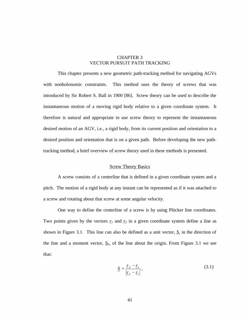
41
CHAPTER 3 VECTOR PURSUIT PATH TRACKING
This chapter presents a new geometric path-tracking method for navigating AGVs
with nonholonomic constraints. This method uses the theory of screws that was
introduced by Sir Robert S. Ball in 1900 [86]. Screw theory can be used to describe the
instantaneous motion of a moving rigid body relative to a given coordinate system. It
therefore is natural and appropriate to use screw theory to represent the instantaneous
desired motion of an AGV, i.e., a rigid body, from its current position and orientation to a
desired position and orientation that is on a given path. Before developing the new path-
tracking method, a brief overview of screw theory used in these methods is presented.
Screw Theory Basics
A screw consists of a centerline that is defined in a given coordinate system and a
pitch. The motion of a rigid body at any instant can be represented as if it was attached to
a screw and rotating about that screw at some angular velocity.
One way to define the centerline of a screw is by using Plücker line coordinates.
Two points given by the vectors r1 and r2 in a given coordinate system define a line as
shown in Figure 3.1. This line can also be defined as a unit vector, S, in the direction of
the line and a moment vector, S0, of the line about the origin. From Figure 3.1 we see
that:
12
12
rr
rrS
−−
= ,
(3.1)
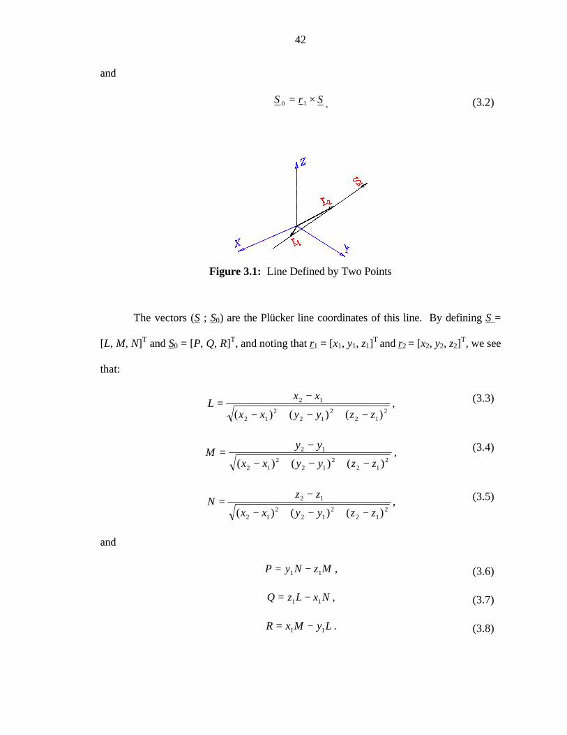
42
and
SrS ×= 10 .
Figure 3.1: Line Defined by Two Points
The vectors (S ; S0) are the Plücker line coordinates of this line. By defining S =
[L, M, N]T and S0 = [P, Q, R]T, and noting that r1 = [x1, y1, z1]T and r2 = [x2, y2, z2]
T, we see
that:
212
212
212
12
)()()( zzyyxx
xxL
−+−+−
−= ,
212
212
212
12
)()()( zzyyxx
yyM
−+−+−
−= ,
212
212
212
12
)()()( zzyyxx
zzN
−+−+−
−= ,
and
MzNyP 11 −= ,
NxLzQ 11 −= ,
LyMxR 11 −= .
(3.2)
(3.3)
(3.4)
(3.5)
(3.6)
(3.7)
(3.8)
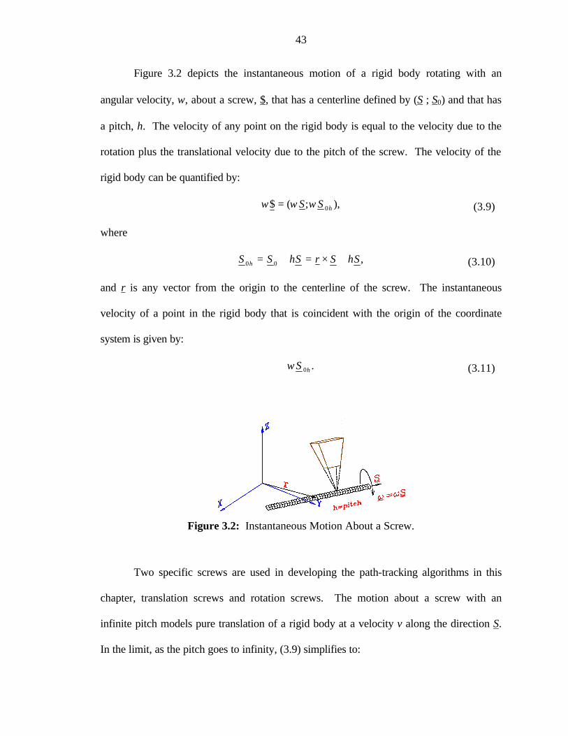
43
Figure 3.2 depicts the instantaneous motion of a rigid body rotating with an
angular velocity, ω, about a screw, $, that has a centerline defined by (S ; S0) and that has
a pitch, h. The velocity of any point on the rigid body is equal to the velocity due to the
rotation plus the translational velocity due to the pitch of the screw. The velocity of the
rigid body can be quantified by:
),;($ 0hSS ωωω =
where
,00 ShSrShSS h +×=+=
and r is any vector from the origin to the centerline of the screw. The instantaneous
velocity of a point in the rigid body that is coincident with the origin of the coordinate
system is given by:
.0hSω
Figure 3.2: Instantaneous Motion About a Screw.
Two specific screws are used in developing the path-tracking algorithms in this
chapter, translation screws and rotation screws. The motion about a screw with an
infinite pitch models pure translation of a rigid body at a velocity v along the direction S.
In the limit, as the pitch goes to infinity, (3.9) simplifies to:
(3.9)
(3.10)
(3.11)

44
);0($ Svv = ,
which is a screw that has a centerline at infinity.
On the other hand, the motion about a screw whose pitch is equal to zero models
pure rotation of a rigid body. By substituting a pitch, h, equal to zero, (3.9) simplifies to:
);($ 0SS ωωω = .
In addition to using rotation and translation screws, a property of instantaneous
screws that proves to be very useful is that they are additive. Note that the units of (3.12)
and (3.13) are the same even though (3.12) is a translation screw and (3.13) is a rotation
screw.
Vector Pursuit
Vector pursuit is a new geometric path-tracking method that uses the theory of
screws. This is a new technique that is developed here and which represents one of the
contributions of this dissertation. It is similar to other geometric methods in that a look-
ahead distance is used to define a current goal point, and then geometry is used to
determine the desired motion of the vehicle. On the other hand, it is different from
current geometric path-tracking methods, such as follow-the-carrot or pure pursuit, which
do not use the orientation at the look-ahead point. Proportional path tracking is a
geometric method that does use the orientation at the look-ahead point. This method
adds the current position error multiplied by some gain to the current orientation error
multiplied by some gain, and therefore becomes geometrically meaningless since terms
with different units are added. Vector pursuit uses both the location and orientation of
the look-ahead point while remaining geometrically meaningful.
(3.12)
(3.13)
45
The first step in vector pursuit calculates two instantaneous screws. The first
instantaneous screw, $t, accounts for the translation from the current vehicle position to
the location of the look-ahead point while the second instantaneous screw, $r, accounts
for the rotation from the current vehicle orientation to the desired orientation at the look-
ahead point. The second step uses the additive property of instantaneous screws to
calculate $d, the sum of $t and $r, which defines the desired instantaneous motion of the
vehicle. Two different methods are considered to calculate the two screws, $t and $r.
The first method initially ignores the nonholonomic constraints of the vehicle to calculate
$t and $r and then deals with the constraints after adding the two instantaneous screws.
Conversely, the second method does not ignore the nonholonomic constraints to calculate
$t and $r. It turns out, for this method, that the sum of $t and $r also does not violate the
nonholonomic constraints. Finally, the last step calculates a desired turning radius, or a
desired turning rate if the current vehicle velocity is considered, from $d.
Defined Coordinate Systems
Before developing the screw theory based path-tracking methods, a few
coordinate systems must first be defined. First, the world coordinate system is defined
where the x-axis points north, the z-axis points down and the y-axis points east to form a
right hand coordinate system. The origin of the world coordinate system defined here is
determined by the conversion from a geodetic coordinate system to a UTM coordinate
system. It is assumed that the desired path is given, or can be converted to, the world
coordinate system. The world coordinate system can be seen in Figure 3.3.
In addition to the world coordinate system, both a moving and the vehicle
coordinate systems are shown in Figure 3.3 also. A moving coordinate system is defined
where the origin is a point on the planned path, the look-ahead point, which is a given

46
distance called the look-ahead distance, L, in front of the orthogonal projection of the
vehicle's position onto the planned path. Its x-axis is oriented in the direction of the
planned path at that point, i.e., the direction from the previous waypoint wi-1 to the current
waypoint wi, the z-axis is down and the y-axis is defined to form a right hand coordinate
system. Since the moving coordinate system’s origin is located at the look-ahead point,
this coordinate system will be referred to as the look-ahead coordinate system. The
selection of the distance L will be discussed later.
wi
wi-1
L
d
WX
WY
θL
VX
θV
VY
L X
L Y
Figure 3.3: Defined Coordinate Systems.
Finally, the vehicle coordinate system is defined where the x-axis is in the
forward direction of the vehicle, the z-axis is down and the y-axis forms a right hand
coordinate system. The origin of the vehicle coordinate system depends on the type of
vehicle. For nonholonomic vehicles, it is defined in a way that decouples the control of
the linear and angular velocities. For example, on a car-like vehicle with rear wheel

47
drive, the origin is defined to be the center of the rear axle. With these three coordinate
systems defined, the development of vector pursuit path tracking is presented now.
A method is required to indicate the coordinate system a vector is referenced
since more than one coordinate system was defined here. Therefore, vectors are written
with a leading superscript indicating the coordinate system to which they are referenced.
Method 1
Recall that this first method initially ignores the nonholonomic constraints of the
vehicle. With this in mind and using (3.12), $t is defined to be:
−−= 0,,;0,0,0$
d
yy
d
xxk V
WL
WV
WL
W
tt
W ,
where d is the distance from the look-ahead point to the vehicle position, (WxL,WyL) are the
coordinates of the look-ahead point in the world coordinate system, and (WxV,WyV) are the
coordinates of the vehicle position in the world coordinate system. The term kt is a
weighting factor that will be dealt with later. Similarly, using (3.13), $r is defined to be:
( ) ,0,,;1,0,0$ VW
VW
rr
W xyk −=
where kr is a weighting factor. Note that the axis of rotation is chosen to be the origin of
the vehicle coordinate system so that no translation is associated with $r. Now the
desired instantaneous screw, $d, is calculated to be:
.0,,;,0,0
$$$
−+−
−+=
+=
d
yykxk
d
xxkykk V
WL
W
tVW
rV
WL
W
tVW
rr
r
W
t
W
d
W
The weighting factors kt and kr are used to control how much the desired
instantaneous screw is influenced by $t and $r, respectively. To determine these
weighting factors it is noted from (3.12) and (3.13) that kt is a linear velocity and kr is an
(3.14)
(3.15)
(3.16)
48
angular velocity. Assuming the vehicle travels on the screw defined by $t at some
velocity, kt = v, the time required for the vehicle to reach the look-ahead point would be:
v
dtt = .
Using the same line of reasoning, if the vehicle travels on the screw defined by $r
at some angular velocity, kr = ω, the time required for the vehicle to rotate from its
current orientation to the orientation at the look-ahead point would be:
ωθθ VL
rt−
= ,
where θL is the angle from the x-axis of the world coordinate system going clockwise to
the x-axis of the look-ahead coordinate system, θV is the angle from the x-axis of the
world coordinate system going clockwise to the x-axis of the vehicle coordinate system,
and their difference must be in the interval (-π,π]. Next, the assumption is made that the
relationship between tt and tr can be defined by:
tr ktt = ,
where k is some positive constant greater than zero. Therefore, the weighting factors can
now be determined from:
vkt = ,
and
( )kd
v
kttk vL
t
VL
r
VLr
θθθθθθω
−=
−=
−== ,
where again, the difference θL-θV must be in the interval (-π,π].
In order to determine the desired motion of the vehicle defined by this
instantaneous screw, the location of its centerline must be determined in the vehicle
(3.17)
(3.18)
(3.19)
(3.20)
(3.21)
49
coordinate system. To do this, the location of the desired instantaneous screw’s
centerline is determined first in the world coordinate system by:
−−
−=
−−=
VL
vW
LW
VWv
WL
W
r
tV
WW yykx
d
yy
k
kxx
d θθ$ ,
and
−−
+=
−+=
VL
vW
LW
VWv
WL
W
r
tV
WW xxky
d
xx
k
kyy
d θθ$ .
Note that equations (3.22) and (3.23) are valid only if kr, i.e. θL-θV, is nonzero. If
kr is nonzero, the location of the desired instantaneous screw’s centerline in the vehicle
coordinate system is determined by:
( ))sin()cos()sin()cos( $$$ VW
VW
VVW
VVWV
dddyxyxx θθθθ +−+= ,
and
( ))cos()sin()cos()sin( $$$ vW
vW
VVW
VVWV
dddyxyxy θθθθ +−−+=− .
Otherwise, if kr is zero, equation (3.16) reduces to equation (3.14), which is a
screw whose centerline in the vehicle coordinate system is located at infinity in a
direction perpendicular to the line that connects the vehicle position and the look-ahead
point.
The desired motion of the vehicle can be determined now that the location of the
desired screw’s centerline is determined in the vehicle coordinate system. An example of
a desired instantaneous screw and its associated desired motion is shown graphically in
Figure 3.4. In this figure, one instantaneous screw is executed continually over time to
exaggerate the desired vehicle motion. From Figure 3.4, it is noted that the initial desired
motion from the current vehicle location is a translation along the vehicle’s negative y-
(3.22)
(3.23)
(3.24)
(3.25)

50
axis and a rotation clockwise. This motion is not possible for a vehicle that is constrained
to translational motion only in the direction of its current orientation. In other words, in
order for the vehicle in Figure 3.4 to translate in the direction of the current vehicle’s
negative y-axis, it must first rotate counter-clockwise. This is opposite of the desired
rotation defined by the instantaneous screw. Therefore, it is noted that the possibility
exists where the vehicle may be unable to execute the motion defined by the desired
instantaneous screw defined in equation (3.16) because of the motion constraints of the
vehicle.
VX ωV$d
Vy$d
Vx$dVY
Figure 3.4: Vehicle Motion if Desired Instantaneous Screw is Continually Executed.
Nonholonomic constraints exist when the motion orthogonal to the vehicle’s
forward direction is not possible. In other words, using the vehicle’s coordinate system
defined earlier, motion is restricted at any instant only in a direction parallel vehicle’s x-
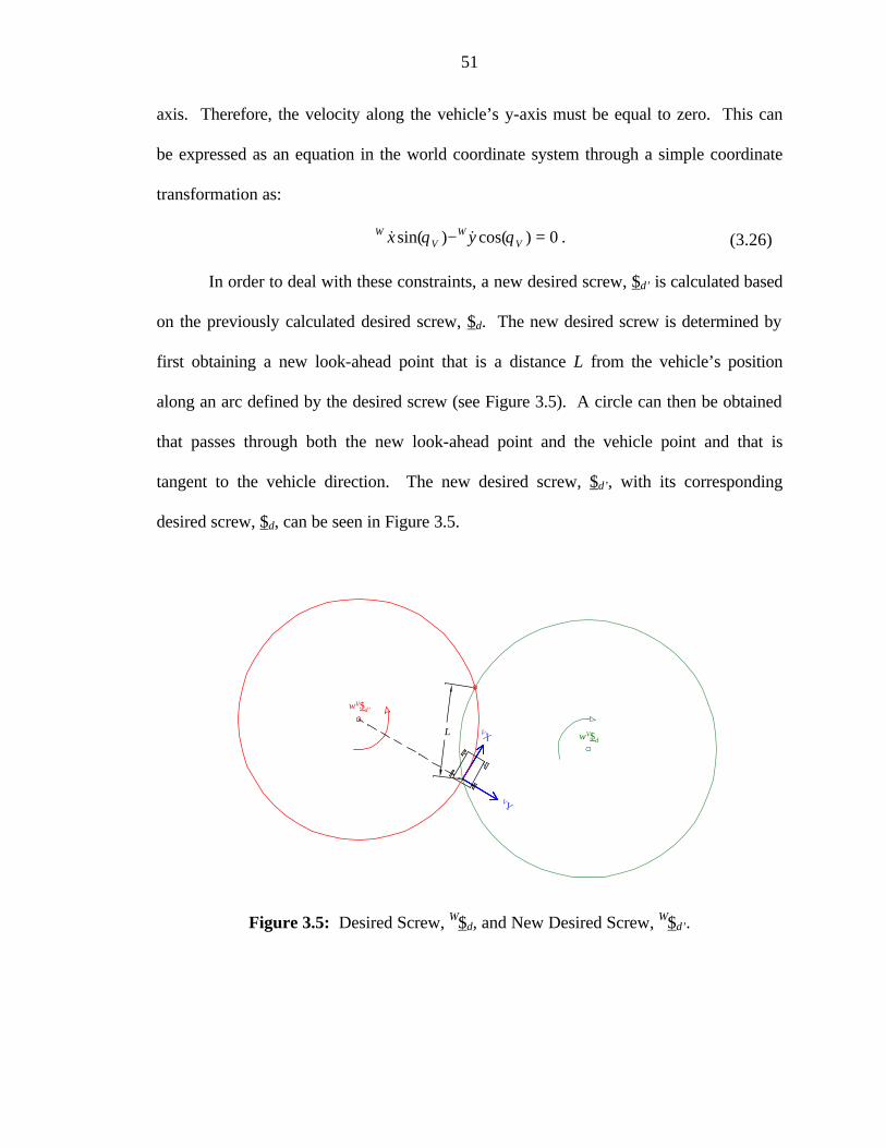
51
axis. Therefore, the velocity along the vehicle’s y-axis must be equal to zero. This can
be expressed as an equation in the world coordinate system through a simple coordinate
transformation as:
0)cos()sin( =− VW
VW yx θθ && .
In order to deal with these constraints, a new desired screw, $d’ is calculated based
on the previously calculated desired screw, $d. The new desired screw is determined by
first obtaining a new look-ahead point that is a distance L from the vehicle’s position
along an arc defined by the desired screw (see Figure 3.5). A circle can then be obtained
that passes through both the new look-ahead point and the vehicle point and that is
tangent to the vehicle direction. The new desired screw, $d’, with its corresponding
desired screw, $d, can be seen in Figure 3.5.
L VX
VY
ωV$d
ωV$d’
Figure 3.5: Desired Screw, W$d, and New Desired Screw, W$d’.
(3.26)

52
Unfortunately, this could place a restriction on the location of $d’s centerline in
order for the new look-ahead point to exist. The distance from the vehicle position to the
centerline of $d must be greater than ½L. This restriction turns out to be a case where the
vehicle needs to simply turn around, and therefore the location of the new desired screw,
$d’, in the vehicle’s reference frame can be determined by the vehicle’s minimum turning
radius rmin using:
0$ =′d
xV
and
min$ ryd
V =′
,
if the direction of the desired screw’s centerline is in the positive z-direction, or:
0$ =′d
xV
and
min$ ryd
V −=′
,
if the direction of the desired screw’s centerline is in the negative z-direction.
If the distance to the centerline of $d is greater than ½L, then two points exist on a
circle whose center is the centerline of $d and whose radius is the distance to the vehicle
position that are a distance L away from the vehicle position. This can be seen in Figure
3.6. In order to determine the location of these two points in the vehicle coordinate
system, the angle from the x-axis of the vehicle coordinate system to the centerline of $d
is determined first by:
( )dd
xy VV$$ ,atan2=α .
(3.27)
(3.28)
(3.29)
(3.30)
(3.31)

53
Next, it is noted through symmetry that the angle between the line from the
vehicle position to p1 and the line from the vehicle position to $d’s centerline is equal to
the angle between the line from the vehicle position to p2 and the line from the vehicle
position to the desired screw’s centerline. Through simple geometry, the magnitude of
this angle can be determined by:
2$
2$2
cos
ddyx
La
VV +=β ,
where β must be in the interval (0,π/2] radians. Now the angle from the x-axis of the
vehicle coordinate system to both p1 and p2 can be determined by:
βαγ ±= .
ωV$dVX
VY
p1
p2
α
β
β
L
L
Figure 3.6: Possible Look-ahead Points p1 and p2.
Only one of these two points is used as the new look-ahead point, so to determine
which point to use, the direction of $d’s centerline is considered. The new look-ahead
(3.32)
(3.33)
54
point is defined to be the point that is encountered first by traveling along the arc defined
by $d starting from the vehicle position. Therefore, if the direction of $d’s centerline is in
the positive z-axis of the vehicle coordinate system, then the angle from the vehicle
coordinate system’s x-axis to the look-ahead point is:
βαγ −= .
This is the case of the desired screw, $d, shown in Figure 3.6 where p1 is determined now
to be the new look-ahead point. Similarly, if the direction of the desired screw’s
centerline is in the negative z-axis of the vehicle reference frame, the angle from the x-
axis of the vehicle coordinate system to the new look-ahead point is:
βαγ += .
Since the angle from x-axis to the new look-ahead point is determined in the
vehicle coordinate system, the location of the new look-ahead point in the vehicle
coordinate system can be calculated by:
)cos(γLxLV = ,
and
)sin(γLyLV = .
Now that the location of the new look-ahead point is known in the vehicle’s
coordinate system, the location of the new desired screw’s centerline can be located in
the vehicle’s coordinate system. Assuming p = p1 or p = p2, from Figure 3.7 we see that
the location of the new desired screw’s centerline is on the vehicle’s y-axis at a distance
R from the x-axis. From Figure 3.7,
222 Rxa pv =+ .
Substituting:
(3.34)
(3.35)
(3.36)
(3.37)
(3.38)

55
pV yRa −= ,
2221 p
Vp
V yLx −= ,
and solving for R gives:
pV y
LR
2
2
= .
Therefore, the new desired screw’s centerline is located at:
0$ =′d
xV ,
pV
V
y
Ly
d 2
2
$ =′
.
ωV$d’
ωV$dVX
VY
R
Vxp
Vyp
a
p
L
Figure 3.7: Locating V$d’’s centerline.
The direction of the new desired screw’s centerline can be determined by the
location of the new look-ahead point in the vehicle’s coordinate system. The direction of
the commanded screw’s centerline depends on which quadrant of the vehicle’s coordinate
system the new look-ahead point is located. This is summarized in Table 3.1.
(3.39)
(3.40)
(3.41)
(3.42)
(3.43)

56
Table 3.1: Desired Screw’s Centerline Direction.
sign of Vxp sign of Vyp Screw’s Centerline Direction
Along the z-axis Positive Positive Positive Positive Negative Negative Negative Positive Negative Negative Negative Positive
Note that when the new look-ahead point’s x-value is negative, the vehicle’s
velocity would have to be negative, or in other words, the vehicle direction would have to
change from forward to reverse. In order to keep the vehicle direction from changing, the
x-value of the look-ahead point must be greater than zero, otherwise the vehicle is
commanded simply to turn around. Equations (3.27) and (3.28) or equations (3.29) and
(3.30) are used again to calculate the location of the commanded screw’s centerline in
this situation.
Finally, it is important to note that the look-ahead distance, L, and the constant k,
are free choices and as such represent parameters that must be selected in order to
optimize or tune the vehicle’s performance.
Method 2
The second method developed to calculate $t and $r takes into account the
vehicle’s nonholonomic constraints. In order to satisfy the constraints, the centerlines of
the instantaneous screws must be on the vehicle’s y-axis and a distance from the x-axis
greater than or equal to the vehicle’s minimum turning radius. The requirement that the
instantaneous screws’ centerlines be a distance greater than or equal to the vehicle’s
minimum turning radius from the x-axis is ignored initially. It is ignored at first because
of the fact that some vehicles, e.g., a differentially driven vehicle, with nonholonomic
constraints have no minimum turning radius. Therefore, the only initial constraint placed

57
on the location of the centerlines of the instantaneous screws is that they must be on the
vehicle’s y-axis. With this in mind, the screw to correct the translational error, $t, was
selected as the center of a circle that passes through the origins of the vehicle coordinate
system and the look-ahead coordinate system and which is tangent to the vehicle’s
current orientation, i.e. the x-axis of the vehicle coordinate system. (See Figure 3.8)
Hence, $t is defined to be:
( ) ( )
+−+= 0,sin
2,cos
2;1,0,0$
22
v
LVv
Wv
LVv
Wtt
W
y
dx
y
dyk θθ ,
where d is the distance from the origin of the vehicle coordinate system to the origin of
the look-ahead coordinate system (where the look-ahead coordinate system is defined as
before), (VxL,VyL) are the coordinates of the look-ahead coordinate system’s origin in the
vehicle coordinate system, (WxV,WyV) are the coordinates of the vehicle position in the
world coordinate system, and θV is the angle from the x-axis of the world coordinate
system to the x-axis of the vehicle coordinate system. The term kt is used again as a
weighting factor that will be dealt with later. Equation (3.44) is valid only if the term VyL
is nonzero. Otherwise, $t is determined by:
−−= 0,,;0,0,0$
d
yy
d
xxk V
WL
WV
WL
W
tt
W .
The instantaneous screw, $r, is defined to be:
( )0,,;1,0,0$ VW
VW
rr
W xyk −= ,
which is the same as equation (3.15), but the weighting factor kr is determined differently.
(3.44)
(3.45)
(3.46)
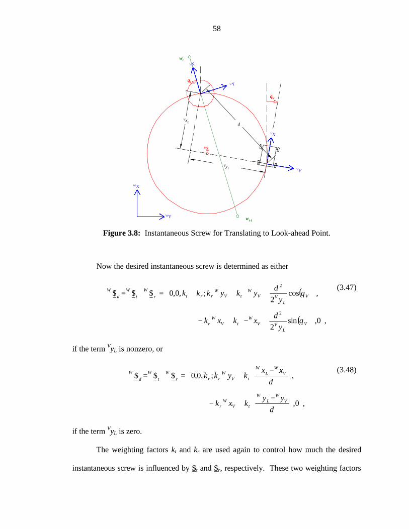
58
VX
VY
W$t
wi-1
wi
WX
WY
θθV
VyL
VxLd
θθL
LX
LY
Figure 3.8: Instantaneous Screw for Translating to Look-ahead Point.
Now the desired instantaneous screw is determined as either
( )
( ) ,0,sin2
,cos2
;,0,0$$$
2
2
+−+−
+++=+=
V
LVV
WtV
Wr
V
LVV
WtV
Wrrtr
W
t
W
d
W
y
dxkxk
y
dykykkk
θ
θ
if the term VyL is nonzero, or
,0,
,;,0,0$$$
−+−
−+=+=
d
yykxk
d
xxkykk
VW
LW
tVW
r
VW
LW
tVW
rrr
W
t
W
d
W
if the term VyL is zero.
The weighting factors kt and kr are used again to control how much the desired
instantaneous screw is influenced by $t and $r, respectively. These two weighting factors
(3.47)
(3.48)

59
are related again by the time required to translate to the look-ahead point and rotate to the
desired orientation. Assuming that the term VyL is nonzero, note that while the
instantaneous screw defined in equation (3.44) describes a motion to translate the vehicle
from its current location to the look-ahead point, it also describes a motion that rotates the
vehicle. This can easily be seen in Figure 3.9. Therefore, from equation (3.13), the
weighting factor kt is an angular velocity now instead of a linear velocity. The amount of
rotation, φ, can be determined by:
( ) ( )( )
−−= 0,
2atan22,2atan2
222
LVL
VL
VL
V
ydyxdyφ .
where φ must be in the interval (0,2π] radians. It is noted that the last part of Equation
(3.49) will always be ±π/2 radians depending only on the sign of VyL.
WX
WY
wi
wi-1
θVθV
VX
VY
VX
VY
φ
Figure 3.9: Rotation defined by $t Instantaneous Screw.
(3.49)

60
The time required to translate from the current vehicle position to the look-ahead
point, assuming that kt = ωt, some angular velocity, is determined by
ttt ω
φ= .
The time required to rotate from the current vehicle orientation to the orientation
at the look-ahead point must also account for the rotation, φ, due to $t. This will either
increase or decrease the time needed to rotate. Assuming kr = ωr, some angular velocity,
this time can be determined by:
( )r
VLrt ω
φθθ −−= .
Again, the assumption is made that the relationship between tt and tr can be
defined by:
,tr ktt =
where k is some positive constant greater than zero. Therefore, the weighting factors can
now be determined from:
ttk ω= ,
and
( ) ( ) ( )( )φ
φθθωφθθφθθω
kkttk VLt
t
VL
r
VLrr
−−=
−−=
−−== .
Using equation (3.47), the centerline of the desired screw can be determined in
the world coordinate system by:
(3.50)
(3.51)
(3.52)
(3.53)
(3.54)

61
( )
( ) ( ) ,cos2)1(
cos2
2
2
$
−+−−=
−=
+
v
LV
VLV
W
v
LV
rt
tV
WW
y
d
k
kx
y
d
kk
kxx
d
θθθφ
φ
θ
and
( )
( ) ( ) .sin2)1(
sin2
2
2
$
−+−+=
+=
+
v
LV
VLV
W
v
LV
rt
tV
WW
y
d
k
ky
y
d
kk
kyy
d
θθθφ
φ
θ
Note that the above calculations of the weighting factors assumed that VyL was
nonzero. If, on the other hand, VyL is zero, then from equation (3.12), the weighting
factor kt is a linear velocity. The amount of time to translate from the current vehicle
position to the look-ahead point at some velocity, kt = v, can be determined by:
v
dtt = .
The time required to rotate from the current vehicle orientation to the orientation
at the look-ahead point can be calculated using equation (3.51) where φ is now zero.
Therefore, assuming kr = ω, some angular velocity, this time can be determined by:
ωθθ VL
rt−
= .
Using equation (3.52) for the relationship between the two times, the weighting
factors can be determined from:
,vkt =
and
( )kd
v
kttk vL
t
VL
r
VLr
θθθθθθω
−=
−=
−== .
(3.55)
(3.56)
(3.57)
(3.58)
(3.59)
(3.60)

62
Using equation (3.48), the centerline of the desired screw can be determined in
the world coordinate system by:
,$
−−
−=
−−=
VL
vW
LW
VWv
WL
W
r
tV
WW yykx
d
yy
k
kxx
d θθ
and
.$
−−
+=
−+=
VL
vW
LW
VWv
WL
W
r
tV
WW xxky
d
xx
k
kyy
d θθ
Finally, using equations (3.24) and (3.25), the centerline of the desired
instantaneous screw can be determined in the vehicle coordinate system to determine the
desired motion of the vehicle. Recall that the vehicle’s nonholonomic constraints were
considered when calculating $t and $r but that the minimum turning radius was ignored.
This has a nice result where Vx$d will always equal zero, which does not break the
nonholonomic constraints. In order to comply with the minimum turning radius
constraint, the magnitude of Vy$d must be greater than or equal to the minimum turning
radius. If it is less than the minimum turning radius, equations (3.27) and (3.28) or
equations (3.29) and (3.30) are used again to calculate the location of the desired screw’s
centerline in the vehicle coordinate system.
As in the first method, the direction of the desired screw’s centerline is
determined by the location of the look-ahead point in the vehicle’s coordinate system and
Table 3.1. Again, when the look-ahead point’s x-value is negative, the vehicle direction
would have to change from forward to reverse. In order to keep the vehicle direction
from changing, the x-value of the look-ahead point must be greater than zero, otherwise
the vehicle is commanded to turn around. Equations (3.27) and (3.28) or equations (3.29)
(3.61)
(3.62)

63
and (3.30) are used again to calculate the location of the commanded screw’s centerline
in this situation.
Finally, it is important to note again that the look-ahead distance, L, and the
constant k, are free choices in this method too and as such represent parameters that must
be selected in order to optimize or tune the vehicle’s performance.
Desired Vehicle Velocity State
The desired velocity-state of the AGV for it to track the given path can now be
determined from the final desired screw calculated from either method 1 or method 2.
The velocity-state is made up of two vectors, a linear velocity vector, v = [vx, vy, vz]T, and
an angular velocity vector, ω = [ωx, ωy, ωz]T, that can represent the motion of any rigid
body in three-dimensional space. In the vehicle coordinate system the linear velocity of
the AGV is limited to the x-axis and the angular velocity is limited to rotation about the
z-axis because of the nonholonomic constraints. Therefore, only the terms vx and ωz need
to be determined. The desired linear velocity, vx, is determined by the desired speed to
follow the path. The user, based on the current mission of the AGV, typically decides
this. The desired angular velocity, ωz, is calculated based on the current location of the
desired screw’s centerline and the current velocity of the AGV. The desired angular
velocity is calculated by:
dy
vVcurrent
z
$
=ω ,
where Vy$d is equal to Vy$d’ for the first method.
Recall that the task of an AGV to accurately track a given path was broken down
into two steps. The first step is to determine the AGV’s desired motion, or velocity state,
(3.63)

64
which was accomplished in this chapter. The second step is to execute the desired
velocity-state. This is the topic of the next chapter.
65
CHAPTER 4 EXECUTION CONTROL
Execution control is the task of executing the AGV’s desired velocity-state as
determined in Chapter 3. After considering the motion constraints of an AGV, the only
two components of an AGV’s velocity-state that can influence the system are vx and ωz.
By carefully choosing the origin of the vehicle’s coordinate system, vx and ωz can be
decoupled allowing for the design of separate controllers. There are a number of
different control techniques that would work here and therefore a design choice must be
made.
Some of the more conventional control techniques include classical control,
proportional-integral-derivative control (PID), adaptive control, and state space methods.
These techniques require a relatively accurate model of the system in order to develop a
satisfactory controller. In addition, these techniques typically restrict the complexity of
the system model (e.g., linearity). Some of the newer control techniques that could be
used here include fuzzy logic control and neural networks. One draw back with neural
network controllers is that they typically require a long learning time where they are
“taught” how to control a system, before they can be effectively used. Fuzzy logic
controllers, on the other hand, do not require a model of the system and do not require a
long learning time. Instead, they rely on the knowledge of an expert on controlling the
particular system. Therefore, with all of this in mind, the proposed controllers of vx and
ωz are both chosen to be fuzzy controllers.
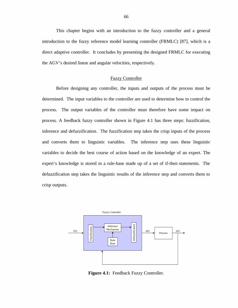
66
This chapter begins with an introduction to the fuzzy controller and a general
introduction to the fuzzy reference model learning controller (FRMLC) [87], which is a
direct adaptive controller. It concludes by presenting the designed FRMLC for executing
the AGV’s desired linear and angular velocities, respectively.
Fuzzy Controller
Before designing any controller, the inputs and outputs of the process must be
determined. The input variables to the controller are used to determine how to control the
process. The output variables of the controller must therefore have some impact on
process. A feedback fuzzy controller shown in Figure 4.1 has three steps: fuzzification,
inference and defuzzification. The fuzzification step takes the crisp inputs of the process
and converts them to linguistic variables. The inference step uses these linguistic
variables to decide the best course of action based on the knowledge of an expert. The
expert’s knowledge is stored in a rule-base made up of a set of if-then statements. The
defuzzification step takes the linguistic results of the inference step and converts them to
crisp outputs.
Fuzzy Controller
InferenceMechanism
RuleBase
Fuzz
ific
atio
n
Def
uzzi
fica
tion
Processr(t) u(t) y(t)
Figure 4.1: Feedback Fuzzy Controller.

67
Fuzzification
Fuzzification is the process of taking a crisp value and converting it to a linguistic
variable. This is accomplished by using membership functions. Membership functions
take a crisp value and map it to a linguistic variable with a value between 0 and 1. For
example, Figure 4.2 shows graphically the membership functions that convert the crisp
value of height, h, to the linguistic variables short, medium and tall. Figure 4.2 shows the
very common triangular membership function with saturated boundaries. From Figure
4.2, a height equal to 5.8 feet gives the linguistic variable “tall” a membership value of
0.8, or µtall(5.8) = 0.8. Similarly, the linguistic variables medium and short would have a
membership values of 0.2 and 0.0, respectively, or µmedium(5.8)= 0.2 and µshort(5.8)= 0.0.
h (feet)
µ
1 2 3 4 5 6 7
shor
t
med
ium
tall
0.5
1.0
Figure 4.2: Height Membership Functions.
A membership function is not limited to being triangular. This can be seen by
other examples of membership functions in Figure 4.3. The choice of the membership
function depends on the application and the designer or the expert. Fuzzification is
therefore a highly subjective process where two different designers may quantify the
same variable differently and both be considered correct.

68
µ
0.5
1.0
µ
0.5
1.0
µ
0.5
1.0
µ
0.5
1.0
Figure 4.3: Possible Fuzzy Membership Functions.
Inference Mechanism
The inference mechanism is made to imitate the expert’s decision process as if he
or she was controlling the process directly. In other words, it interprets the current state
of the process and then uses its knowledge of the plant to decide the best way to control
the plant.
The knowledge of how to control the plant is represented by creating a rule-base
of if <premise>, then <consequent> statements. Take, for example, the inverted
pendulum problem shown in Figure 4.4a. It is desired to balance the pendulum in a
vertical position by controlling the force F. Suppose that the angular error, θ, from the
vertical and its derivative are measured and used as inputs. Using the membership
functions shown in Figure 4.4b, one rule may be, if the error is “Positive Small” (PS) and
the change in error is “Negative Large” (NL), then the force is “Positive Medium” (PM).
A second rule may be if the error is “Zero” (Z) and the change in error is “Positive
Small” (PS), then the force is “Negative Small” (NS). A rule for each possible
combination of error and change in error can be determined similarly. If the number of
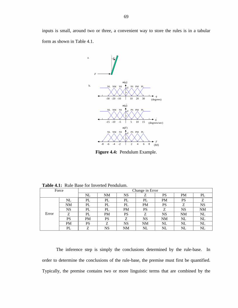
69
inputs is small, around two or three, a convenient way to store the rules is in a tabular
form as shown in Table 4.1.
F
θa.
NL NM NS PS PM PLZ
NL NM NS PS PM PLZ
NL NM NS PS PM PLZ
b.µ(θ)
µ(θ).
µ(F)
θ(degrees)
θ(degrees/sec)
.
F(lbf)
-30 -20 -10 10 20 30
-15 -10 -5 5 10 15
-8 -6 -4 -2 2 4 6 8
Figure 4.4: Pendulum Example.
Table 4.1: Rule Base for Inverted Pendulum. Change in Error Force
NL NM NS Z PS PM PL NL PL PL PL PL PM PS Z NM PL PL PL PM PS Z NS NS PL PL PM PS Z NS NM Z PL PM PS Z NS NM NL PS PM PS Z NS NM NL NL PM PS Z NS NM NL NL NL
Error
PL Z NS NM NL NL NL NL
The inference step is simply the conclusions determined by the rule-base. In
order to determine the conclusions of the rule-base, the premise must first be quantified.
Typically, the premise contains two or more linguistic terms that are combined by the
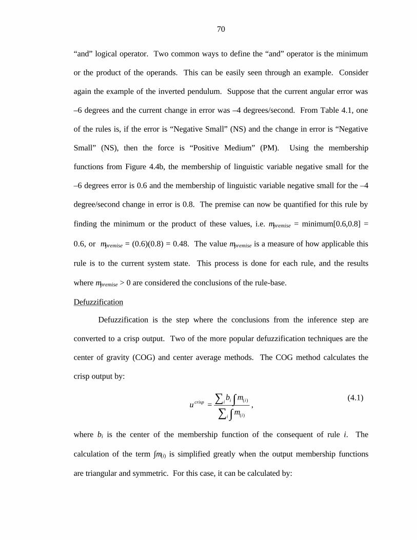
70
(4.1)
“and” logical operator. Two common ways to define the “and” operator is the minimum
or the product of the operands. This can be easily seen through an example. Consider
again the example of the inverted pendulum. Suppose that the current angular error was
–6 degrees and the current change in error was –4 degrees/second. From Table 4.1, one
of the rules is, if the error is “Negative Small” (NS) and the change in error is “Negative
Small” (NS), then the force is “Positive Medium” (PM). Using the membership
functions from Figure 4.4b, the membership of linguistic variable negative small for the
–6 degrees error is 0.6 and the membership of linguistic variable negative small for the –4
degree/second change in error is 0.8. The premise can now be quantified for this rule by
finding the minimum or the product of these values, i.e. µpremise = minimum[0.6,0.8] =
0.6, or µpremise = (0.6)(0.8) = 0.48. The value µpremise is a measure of how applicable this
rule is to the current system state. This process is done for each rule, and the results
where µpremise > 0 are considered the conclusions of the rule-base.
Defuzzification
Defuzzification is the step where the conclusions from the inference step are
converted to a crisp output. Two of the more popular defuzzification techniques are the
center of gravity (COG) and center average methods. The COG method calculates the
crisp output by:
∑ ∫∑ ∫=
i i
i iicrispb
u)(
)(
µ
µ,
where bi is the center of the membership function of the consequent of rule i. The
calculation of the term ∫µ(i) is simplified greatly when the output membership functions
are triangular and symmetric. For this case, it can be calculated by:

71
∫
−=
2
2
)()(
)(
i
i
premise
premisei wµ
µµ ,
where w is the width of the base of the triangle.
The center average method calculates the crisp output by:
∑∑
=i premise
i premiseicrisp
i
ib
u)(
)(
µ
µ.
Continuing with the inverted pendulum example where the angular error was –6
degrees and the change in error was –4 degrees/second, using equation (4.1) and using
the minimum function to quantify the premise of each rule gives a crisp output of:
44.272.028.172.068.1
)72.0)(0()28.1)(2()72.0)(2()68.1)(4(=
++++++
=crispu .
Finally, using equation (4.3) and the minimum function to quantify the premise of each
rule gives a crisp output of:
57.22.04.02.06.0
)2.0)(0()4.0)(2()2.0)(2()6.0)(4(=
++++++
=crispu .
Fuzzy Reference Model Learning Control [86]
There are two general techniques for adaptive control, direct and indirect. Direct
adaptive control, shown in Figure 4.5, monitors a system’s response and then modifies
the controller in order to achieve a specified desired performance. On the other hand,
indirect adaptive control monitors a system’s response in order to identify parameters of
the system’s model. The controller is designed as a function of these model parameters
to achieve a specified desired performance. A block diagram of an indirect adaptive
controller is shown in Figure 4.6. Fuzzy reference model learning control (FRMLC) is a
direct adaptive controller.
(4.2)
(4.3)
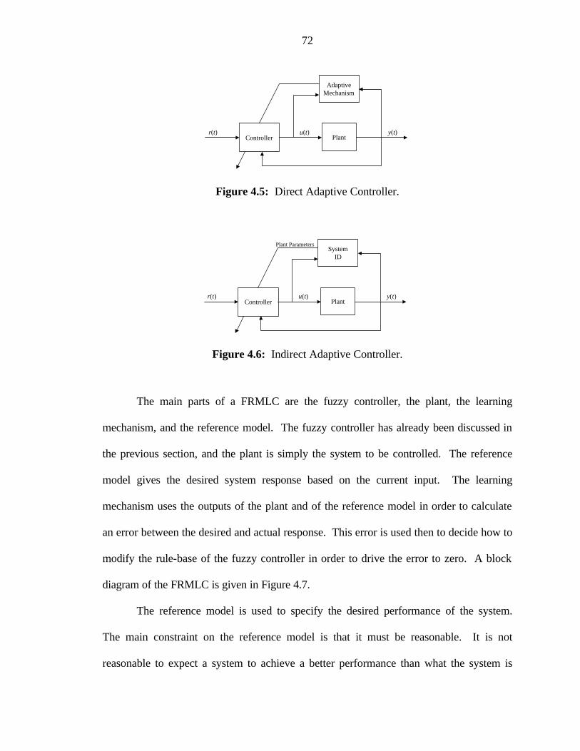
72
AdaptiveMechanism
Controller Plantr(t) u(t) y(t)
Figure 4.5: Direct Adaptive Controller.
SystemID
Controller Plantr(t) u(t) y(t)
Plant Parameters
Figure 4.6: Indirect Adaptive Controller.
The main parts of a FRMLC are the fuzzy controller, the plant, the learning
mechanism, and the reference model. The fuzzy controller has already been discussed in
the previous section, and the plant is simply the system to be controlled. The reference
model gives the desired system response based on the current input. The learning
mechanism uses the outputs of the plant and of the reference model in order to calculate
an error between the desired and actual response. This error is used then to decide how to
modify the rule-base of the fuzzy controller in order to drive the error to zero. A block
diagram of the FRMLC is given in Figure 4.7.
The reference model is used to specify the desired performance of the system.
The main constraint on the reference model is that it must be reasonable. It is not
reasonable to expect a system to achieve a better performance than what the system is

73
capable of achieving. Every system has its limitations, and these limitations must be
considered when choosing the reference model.
InferenceMechanism
RuleBase
Fuzz
ific
atio
n
Def
uzzi
fica
tion
InferenceMechanism
RuleBase
Fuzz
ific
atio
n
Def
uzzi
fica
tion
Fuzzy Controller
Fuzzy Inverse Model
ReferenceModel
Process
Rule-baseModifier
+
–
Learning Mechanism
p(kT) e(kT)
r(kT) u(kT) y(kT)
Figure 4.7: FRMLC Block Diagram.
Once the reference model is determined, a discrete error signal is calculated by:
)()()( kTykTykTe m −= ,
where e(kT) is the current error, ym(kT) is the output of the reference model, y(kT) is the
output of the system, and T is the sample time. Depending on the system characteristics,
it may also be useful to calculate the discrete change in error by:
T
TkTekTekTc
)()()(
−−= ,
where c(kT) is the change in error, e(kT) is the current error from equation (4.4), and
e(kT-T) is the error calculated on the previous time sample. Then, these results and any
(4.4)
(4.5)
74
other system data are used to determine the necessary changes to the process inputs,
p(kT), by the learning mechanism.
The learning mechanism is made up of a fuzzy inverse model and a rule-base
modifier. The purpose of the fuzzy inverse model is to take the calculations e(kT) and
c(kT) and determine how to change the process input, u(kT), in order to drive e(kT) to
zero. The output of the fuzzy inverse model is the desired change in process input and is
represented by p(kT). First, the inputs are fuzzified by membership functions specified
by the designer. The inference mechanism then uses rules such as, if the error is
“positive small” and the change in error is “zero,” then the change in process input is
“negative small.” It is referred to as the fuzzy inverse model because these rules typically
depend on the plant dynamics. Finally, the output, p(kT), is defuzzified by the COG,
center-average or some other defuzzification technique. Then the output, p(kT), is used
to modify the controllers rule-base.
The fuzzy controller’s rule-base is modified by first determining which rules are
active. In other words, determine which rule’s certainty is greater than zero:
0)(
>ipremiseµ .
Then, for all the rules that are active, the center of the mth output membership function is
adjusted by:
)()()( kTpTkTbkTb mm +−= ,
where bm(kT) is the current center of the mth output membership function, bm(kT-T) is the
center of the mth output membership function at the previous time sample, and p(kT) is
the desired change in process input that was calculated by the inverse model.
(4.6)
(4.7)
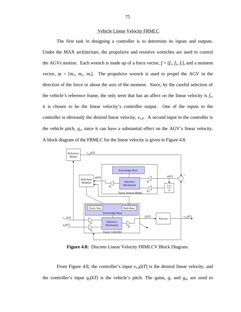
75
Vehicle Linear Velocity FRMLC
The first task in designing a controller is to determine its inputs and outputs.
Under the MAX architecture, the propulsive and resistive wrenches are used to control
the AGVs motion. Each wrench is made up of a force vector, f = [fx, fy, fz], and a moment
vector, m = [mx, my, mz]. The propulsive wrench is used to propel the AGV in the
direction of the force or about the axis of the moment. Since, by the careful selection of
the vehicle’s reference frame, the only term that has an affect on the linear velocity is fx,
it is chosen to be the linear velocity’s controller output. One of the inputs to the
controller is obviously the desired linear velocity, vx,d. A second input to the controller is
the vehicle pitch, θy, since it can have a substantial effect on the AGV’s linear velocity.
A block diagram of the FRMLC for the linear velocity is given in Figure 4.8.
InferenceMechanism
Fuzzy Controller
Fuzzy Inverse Model
ReferenceModel
Process
Rule-baseModifier
+
–
p(kT) e(kT)
vx,d(kT) fx(kT) vx,a(kT)
InferenceMechanism
gv
gθ
θy(kT) gf
Knowledge-Base
Fuzzy Sets Rule-Base
vx,m(kT)
Knowledge-Base
ge
gce
gp 1-z-1
T
Figure 4.8: Discrete Linear Velocity FRMLCV Block Diagram.
From Figure 4.8, the controller’s input vx,d(kT) is the desired linear velocity, and
the controller’s input θy(kT) is the vehicle’s pitch. The gains, gv and gθ, are used to

76
normalize the inputs. By doing this, both inputs are fuzzified using the membership
functions given in Figure 4.9. Therefore, the gain gv is chosen to be 1/vmax, where vmax is
the maximum velocity of the AGV, and the gain gθ is chosen to be 1/θy,max, where θy,max is
the maximum allowable pitch. Both of these terms, the maximum AGV velocity and the
maximum allowable pitch, are available from the VCU configuration message under the
MAX architecture.
µ
0.2 0.4 0.6 0.8 1.0-1.0 -0.8 -0.6 -0.4 -0.2
P1 P2 P3 P4 P5N5 N4 N3 N2 N1 Z
Figure 4.9: Normalized Input Membership Functions.
The controller’s output in Figure 4.8 fx(kT) is the first term in the propulsive
wrench. Using the output membership functions shown in Figure 4.10, the output of the
inference mechanism is normalized also. The gain gf is used to scale this output to allow
the controller to command the entire range of the term fx. In the MAX architecture, the
term fx has the range from –100 to 100 percent, and therefore the gain gf is chosen to be
100.
µ
0.2 0.4 0.6 0.8 1.0-1.0 -0.8 -0.6 -0.4 -0.2
P1 P2 P3 P4 P5N5 N4 N3 N2 N1 Z
Figure 4.10: Normalized Output Membership Functions.
Now that the inputs and the output of the fuzzy controller are defined, the rule-
base for the inference mechanism must be defined. Typically, if little or nothing is

77
known about the plant’s characteristics, each rule’s consequent is initialized to the
linguistic variable “zero.” This requires the controller to completely learn the system it is
trying to control. By using the MAX architecture, an important conclusion about the
plant’s characteristics can be made. This conclusion is that increasing the term fx should
have the general characteristic of increasing vx, and decreasing the term fx should have the
general characteristic of decreasing vx. With this in mind, and using the membership
function defined in Figures 4.9 and 4.10, the rule base for the fuzzy controller is
initialized with the rules given in Table 4.2.
Table 4.2: Linear Velocity Initial Rule-Base Desired Linear Velocity Force
N5 N4 N3 N2 N1 Z P1 P2 P3 P4 P5 N5 N5 N4 N3 N2 N1 Z P1 P2 P3 P4 P5 N4 N5 N4 N3 N2 N1 Z P1 P2 P3 P4 P5 N3 N5 N4 N3 N2 N1 Z P1 P2 P3 P4 P5 N2 N5 N4 N3 N2 N1 Z P1 P2 P3 P4 P5 N1 N5 N4 N3 N2 N1 Z P1 P2 P3 P4 P5 Z N5 N4 N3 N2 N1 Z P1 P2 P3 P4 P5 P1 N5 N4 N3 N2 N1 Z P1 P2 P3 P4 P5 P2 N5 N4 N3 N2 N1 Z P1 P2 P3 P4 P5 P3 N5 N4 N3 N2 N1 Z P1 P2 P3 P4 P5 P4 N5 N4 N3 N2 N1 Z P1 P2 P3 P4 P5
Pitch
P5 N5 N4 N3 N2 N1 Z P1 P2 P3 P4 P5
It is assumed in Table 4.2 that the pitch has no affect on the control of the AGV’s
linear velocity. This assumption is made initially because there is not enough
information about the plant’s characteristics to make a conclusion on how the pitch will
affect the control of the AGV’s linear velocity. Therefore, the controller must learn how
to control the plant for different vehicle pitches.
The reference model takes the desired linear velocity as input and outputs an
estimate of what the vehicle linear velocity should be. The model implemented here is a
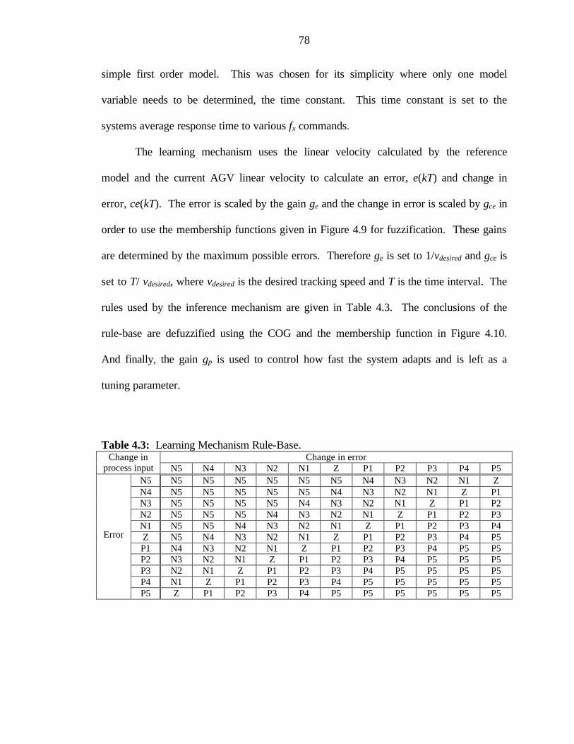
78
simple first order model. This was chosen for its simplicity where only one model
variable needs to be determined, the time constant. This time constant is set to the
systems average response time to various fx commands.
The learning mechanism uses the linear velocity calculated by the reference
model and the current AGV linear velocity to calculate an error, e(kT) and change in
error, ce(kT). The error is scaled by the gain ge and the change in error is scaled by gce in
order to use the membership functions given in Figure 4.9 for fuzzification. These gains
are determined by the maximum possible errors. Therefore ge is set to 1/vdesired and gce is
set to T/ vdesired, where vdesired is the desired tracking speed and T is the time interval. The
rules used by the inference mechanism are given in Table 4.3. The conclusions of the
rule-base are defuzzified using the COG and the membership function in Figure 4.10.
And finally, the gain gp is used to control how fast the system adapts and is left as a
tuning parameter.
Table 4.3: Learning Mechanism Rule-Base. Change in error Change in
process input N5 N4 N3 N2 N1 Z P1 P2 P3 P4 P5 N5 N5 N5 N5 N5 N5 N5 N4 N3 N2 N1 Z N4 N5 N5 N5 N5 N5 N4 N3 N2 N1 Z P1 N3 N5 N5 N5 N5 N4 N3 N2 N1 Z P1 P2 N2 N5 N5 N5 N4 N3 N2 N1 Z P1 P2 P3 N1 N5 N5 N4 N3 N2 N1 Z P1 P2 P3 P4 Z N5 N4 N3 N2 N1 Z P1 P2 P3 P4 P5 P1 N4 N3 N2 N1 Z P1 P2 P3 P4 P5 P5 P2 N3 N2 N1 Z P1 P2 P3 P4 P5 P5 P5 P3 N2 N1 Z P1 P2 P3 P4 P5 P5 P5 P5 P4 N1 Z P1 P2 P3 P4 P5 P5 P5 P5 P5
Error
P5 Z P1 P2 P3 P4 P5 P5 P5 P5 P5 P5

79
Vehicle Angular Velocity FRMLC
The angular velocity FRMLC uses the block diagram given in Figure 4.11, which
is very similar to the linear velocity FRMLC block diagram. Here the controller
reference input, ωz,d(kT), is the current desired angular velocity, and the input v(kT) is the
vehicle’s current linear velocity. The linear velocity is chosen as an input since it is
expected that more slip will occur between the vehicle tires and the ground at higher
speeds, and therefore affect the vehicle’s angular velocity. The gains, gω and gv, are used
again to normalize the inputs. The gain gω is chosen to be 1/ωz,max, where ωz,max is the
vehicle’s maximum angular velocity. Similarly, the gain gv is chosen to be 1/vmax where
vmax is the vehicle’s maximum linear velocity. Again, the information required in order
to calculate these gains are given either by the Vehicle Control Unit (VCU) configuration
report or measured by the Position system (POS).
InferenceMechanism
Fuzzy Controller
Fuzzy Inverse Model
ReferenceModel
Process
Rule-baseModifier
+
–
p(kT) e(kT)
ωz,d(kT) mz(kT) ωz,a(kT)
InferenceMechanism
gω
gv
vx(kT) gm
Knowledge-Base
Fuzzy Sets Rule-Base
ωz,m(kT)
Knowledge-Base
ge
gce
gp 1-z-1
T
Figure 4.11: Angular Velocity FRMLC Block Diagram.

80
For vehicles with a nonzero minimum turning radius, ωz,max turns out to be a
function of the AGV’s current linear velocity and its minimum turning radius:
minmax, r
vcurrentz =ω .
Note that when the current linear velocity is equal to zero, the gain gω for vehicles with a
nonzero minimum turning radius is infinite. This is because the vehicle is not capable of
turning unless the linear velocity is nonzero. Since it is impossible for the vehicle to turn
unless the linear velocity is nonzero, the gain gω is set to zero if the linear velocity is
zero. This is done so that the controller does not attempt to adapt for this case.
The controller’s output in Figure 4.11 mz(kT) is the last term of the propulsive
wrench. Using the output membership functions shown in Figure 4.10, the output of the
inference mechanism is normalized. The gain gm is used to scale this output to allow the
controller to command the entire range of the term mz. In the MAX architecture, the term
mz also has the range from –100 to 100 percent, and therefore the gain gm is chosen to be
100.
Just as the MAX architecture provided information for the linear velocity
controller, it also provides some information about the angular velocity in order to
initialize the rule-base of its controller. It is expected that by increasing the term mz in
the propulsive wrench, the AGVs angular velocity will increase. And, by decreasing the
term mz in the propulsive wrench, the AGVs angular velocity will decrease. This is, of
course, with the exception when the linear velocity is equal to zero as mentioned earlier.
With this information, and using the membership functions defined in Figures 4.9 and
4.10, the rule-base for the angular velocity controller is initialized with the rules given in
Table 4.4.
(4.8)
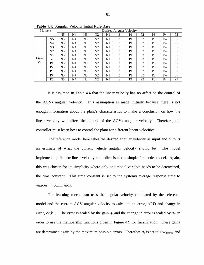
81
Table 4.4: Angular Velocity Initial Rule-Base Desired Angular Velocity Moment
N5 N4 N3 N2 N1 Z P1 P2 P3 P4 P5 N5 N5 N4 N3 N2 N1 Z P1 P2 P3 P4 P5 N4 N5 N4 N3 N2 N1 Z P1 P2 P3 P4 P5 N3 N5 N4 N3 N2 N1 Z P1 P2 P3 P4 P5 N2 N5 N4 N3 N2 N1 Z P1 P2 P3 P4 P5 N1 N5 N4 N3 N2 N1 Z P1 P2 P3 P4 P5 Z N5 N4 N3 N2 N1 Z P1 P2 P3 P4 P5 P1 N5 N4 N3 N2 N1 Z P1 P2 P3 P4 P5 P2 N5 N4 N3 N2 N1 Z P1 P2 P3 P4 P5 P3 N5 N4 N3 N2 N1 Z P1 P2 P3 P4 P5 P4 N5 N4 N3 N2 N1 Z P1 P2 P3 P4 P5
Linear Vel.
P5 N5 N4 N3 N2 N1 Z P1 P2 P3 P4 P5
It is assumed in Table 4.4 that the linear velocity has no affect on the control of
the AGVs angular velocity. This assumption is made initially because there is not
enough information about the plant’s characteristics to make a conclusion on how the
linear velocity will affect the control of the AGVs angular velocity. Therefore, the
controller must learn how to control the plant for different linear velocities.
The reference model here takes the desired angular velocity as input and outputs
an estimate of what the current vehicle angular velocity should be. The model
implemented, like the linear velocity controller, is also a simple first order model. Again,
this was chosen for its simplicity where only one model variable needs to be determined,
the time constant. This time constant is set to the systems average response time to
various mz commands.
The learning mechanism uses the angular velocity calculated by the reference
model and the current AGV angular velocity to calculate an error, e(kT) and change in
error, ce(kT). The error is scaled by the gain ge and the change in error is scaled by gce in
order to use the membership functions given in Figure 4.9 for fuzzification. These gains
are determined again by the maximum possible errors. Therefore ge is set to 1/ωdesired and

82
gce is set to T/ωdesired, where ωdesired is the desired angular velocity and T is the time
interval. The rules used by the inference mechanism are given in Table 4.3. The
conclusions of the rule-base are defuzzified using the COG and the membership function
in Figure 4.10. And finally, the gain gp is used to control how fast the system adapts and
is again left as a tuning parameter.
83
CHAPTER 5 RESULTS
The new path-tracking algorithm developed in this dissertation, vector pursuit, is
a geometric technique. Geometric techniques use a look-ahead point, which is on the
path at a distance L ahead of the orthogonal projection of the vehicle’s position onto the
path, to determine the desired motion of the vehicle. Unfortunately, there is a tradeoff in
determining the distance L. Increasing L tends to dampen the system leading to a stable
system with less oscillation. On the other hand, increasing L also tends to cause the
vehicle to cut corners of a path. Therefore, it is desirable to have a small look-ahead
distance in order to accurately navigate the path, but out of necessity, a large value
typically is used to achieve a stable system with little oscillation.
A factor that must be considered when choosing the look-ahead distance is the
vehicle speed. As the vehicle speed increases, the look-ahead distance typically needs to
be increased, too. Having a look-ahead distance greater than zero allows the vehicle to
start turning before it actually reaches a curve in the path. Starting the turn early is
desirable because of the fact that a certain amount of time is required for the vehicle to
execute a commanded turning rate. The faster the vehicle is going, the sooner the vehicle
needs to start its turn.
Ideally then, a geometric path-tracking technique would allow small look-ahead
distances to accurately track the given path, and not be sensitive to small changes in
vehicle speed. This chapter presents the results of tests done to determine vector
pursuit’s ability to track paths accurately with different look-ahead distances and at
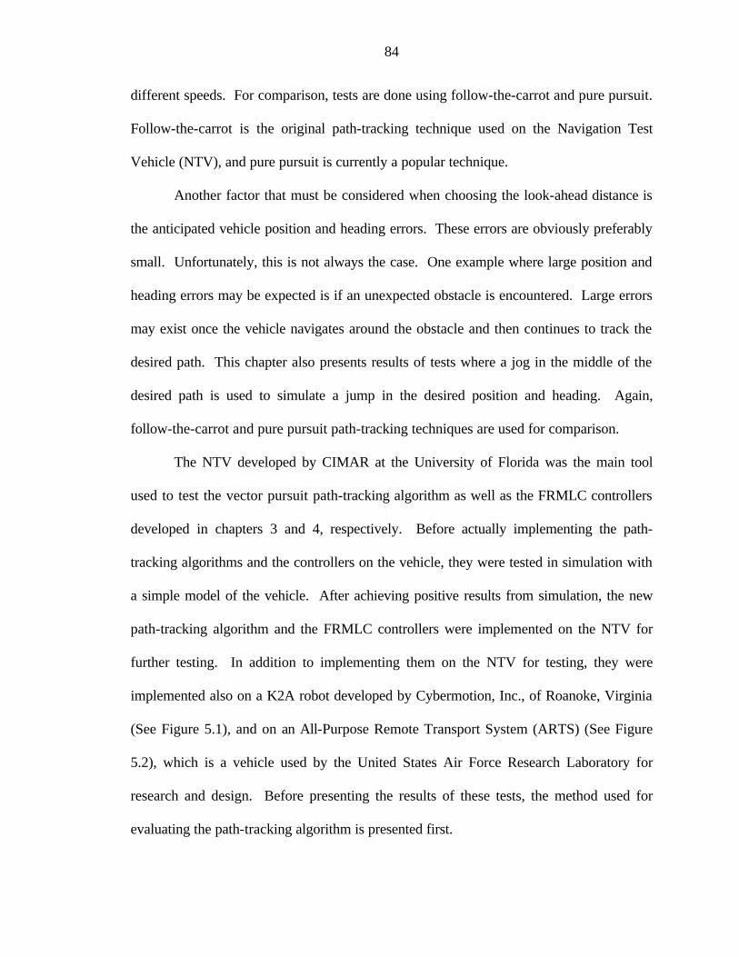
84
different speeds. For comparison, tests are done using follow-the-carrot and pure pursuit.
Follow-the-carrot is the original path-tracking technique used on the Navigation Test
Vehicle (NTV), and pure pursuit is currently a popular technique.
Another factor that must be considered when choosing the look-ahead distance is
the anticipated vehicle position and heading errors. These errors are obviously preferably
small. Unfortunately, this is not always the case. One example where large position and
heading errors may be expected is if an unexpected obstacle is encountered. Large errors
may exist once the vehicle navigates around the obstacle and then continues to track the
desired path. This chapter also presents results of tests where a jog in the middle of the
desired path is used to simulate a jump in the desired position and heading. Again,
follow-the-carrot and pure pursuit path-tracking techniques are used for comparison.
The NTV developed by CIMAR at the University of Florida was the main tool
used to test the vector pursuit path-tracking algorithm as well as the FRMLC controllers
developed in chapters 3 and 4, respectively. Before actually implementing the path-
tracking algorithms and the controllers on the vehicle, they were tested in simulation with
a simple model of the vehicle. After achieving positive results from simulation, the new
path-tracking algorithm and the FRMLC controllers were implemented on the NTV for
further testing. In addition to implementing them on the NTV for testing, they were
implemented also on a K2A robot developed by Cybermotion, Inc., of Roanoke, Virginia
(See Figure 5.1), and on an All-Purpose Remote Transport System (ARTS) (See Figure
5.2), which is a vehicle used by the United States Air Force Research Laboratory for
research and design. Before presenting the results of these tests, the method used for
evaluating the path-tracking algorithm is presented first.
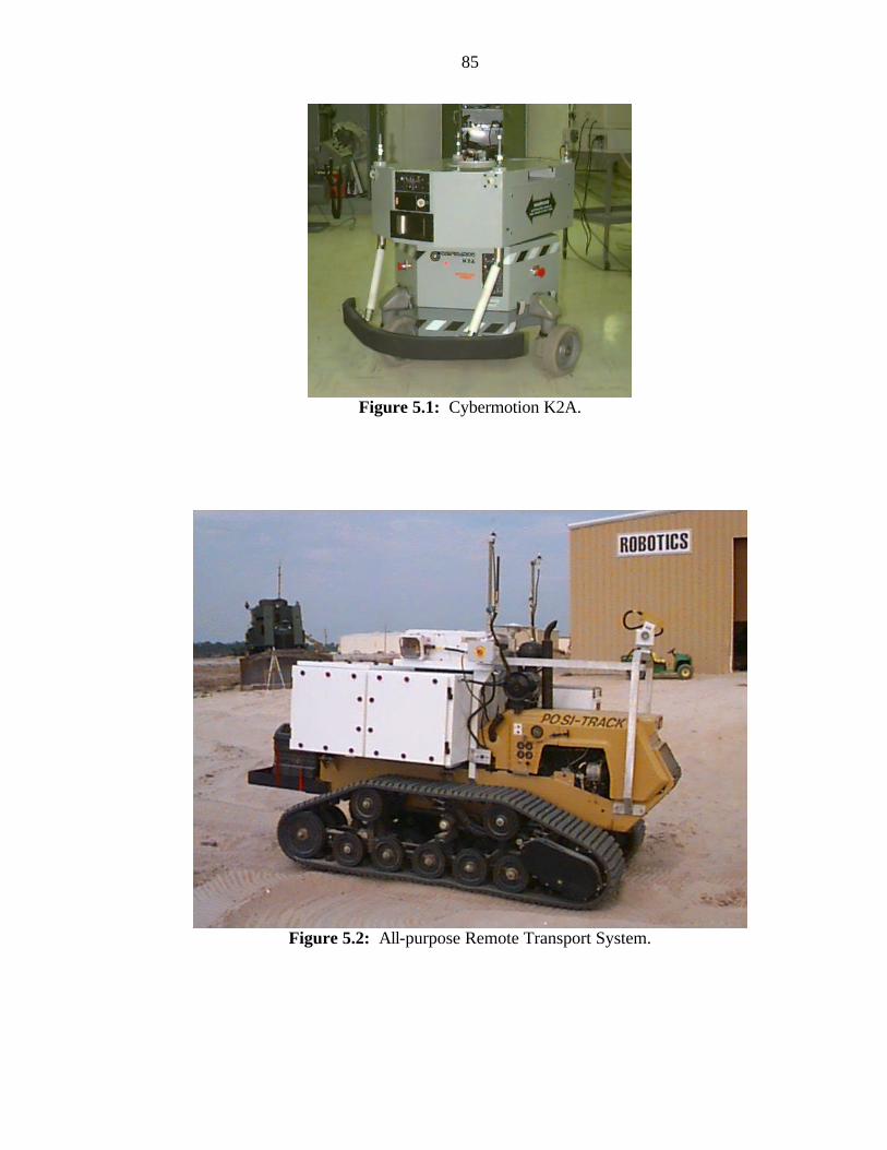
85
Figure 5.1: Cybermotion K2A.
Figure 5.2: All-purpose Remote Transport System.
86
(5.1)
Method for Evaluating Path Tracking
In order to evaluate the path-tracking algorithm, two errors are measured. A
position error and a heading error are measured for every new position data from the POS
module. These errors are calculated relative to a coordinate system that is defined to
have its origin located at the perpendicular projection of the current vehicle location onto
the planned path. Its x-axis is orientated with the path direction at that point, its z-axis is
down, and its y-axis forms a right hand coordinate system. This coordinate system,
referred to as the perpendicular coordinate system, as well as the position and heading
errors, are shown graphically in Figure 5.3. Then the position error, e, is defined to be:
vP ye= ,
where (PxV,PyV) are the coordinates of the vehicle position in the perpendicular coordinate
system defined above. Note that by the definition of this coordinate system, PxV always
equals zero. Next, the heading error, θe, is defined to be:
VPe θθθ −= ,
where θP is the angle from the x-axis of the world coordinate system to the x-axis of the
perpendicular coordinate system, θV is the angle from the x-axis of the world coordinate
system to the x-axis of the vehicle coordinate system, and θe is in the interval (-π,π].
Navigation Test Vehicle (NTV)
This section first presents the results of testing the vector pursuit path-tracking
algorithm and the fuzzy reference model learning controllers in simulation and then
presents the implementation results. It concludes with the results of tests done where the
NTV is driving backwards.
(5.2)

87
VX
VY
θθV
θθP
PX
P Y
wi-1
wi
WX
WY
e
Figure 5.3: Defining Position and Heading Errors.
Simulation Model
Using the world and vehicle coordinate systems defined in Chapter 3, a kinematic
model of the NTV is given by the following equations:
)cos( VVW vx θ=& ,
)sin( VVW vy θ=& ,
and
W
vV
)tan(φθ =& ,
where WxV and WyV give the vehicle position, θV is the vehicle heading, v is the vehicle
speed, φ is the steering wheel angle and W is the vehicle’s wheelbase.
Recall that the outputs of the controllers designed in Chapter 4 are the percent
force along the vehicle’s x-axis and the percent moment about the vehicle’s z-axis. On
the NTV, the magnitude of percent force maps directly to the percent of the maximum
(5.3)
(5.4)
(5.5)
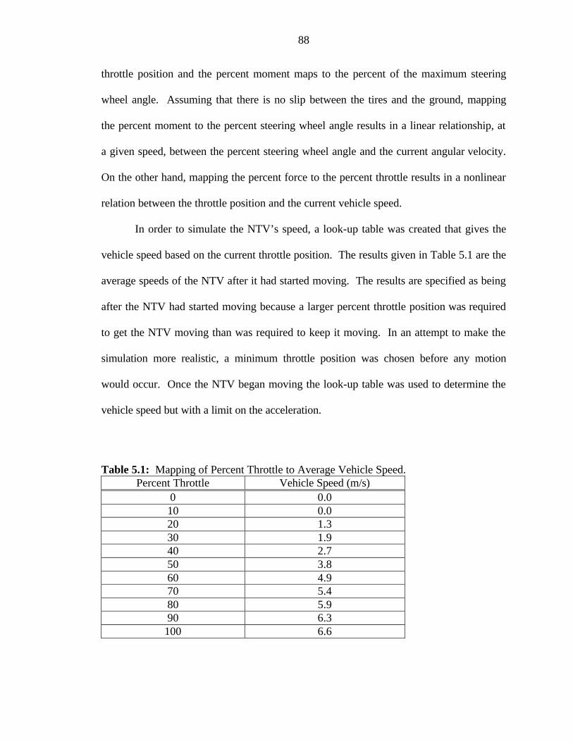
88
throttle position and the percent moment maps to the percent of the maximum steering
wheel angle. Assuming that there is no slip between the tires and the ground, mapping
the percent moment to the percent steering wheel angle results in a linear relationship, at
a given speed, between the percent steering wheel angle and the current angular velocity.
On the other hand, mapping the percent force to the percent throttle results in a nonlinear
relation between the throttle position and the current vehicle speed.
In order to simulate the NTV’s speed, a look-up table was created that gives the
vehicle speed based on the current throttle position. The results given in Table 5.1 are the
average speeds of the NTV after it had started moving. The results are specified as being
after the NTV had started moving because a larger percent throttle position was required
to get the NTV moving than was required to keep it moving. In an attempt to make the
simulation more realistic, a minimum throttle position was chosen before any motion
would occur. Once the NTV began moving the look-up table was used to determine the
vehicle speed but with a limit on the acceleration.
Table 5.1: Mapping of Percent Throttle to Average Vehicle Speed. Percent Throttle Vehicle Speed (m/s)
0 0.0 10 0.0 20 1.3 30 1.9 40 2.7 50 3.8 60 4.9 70 5.4 80 5.9 90 6.3
100 6.6
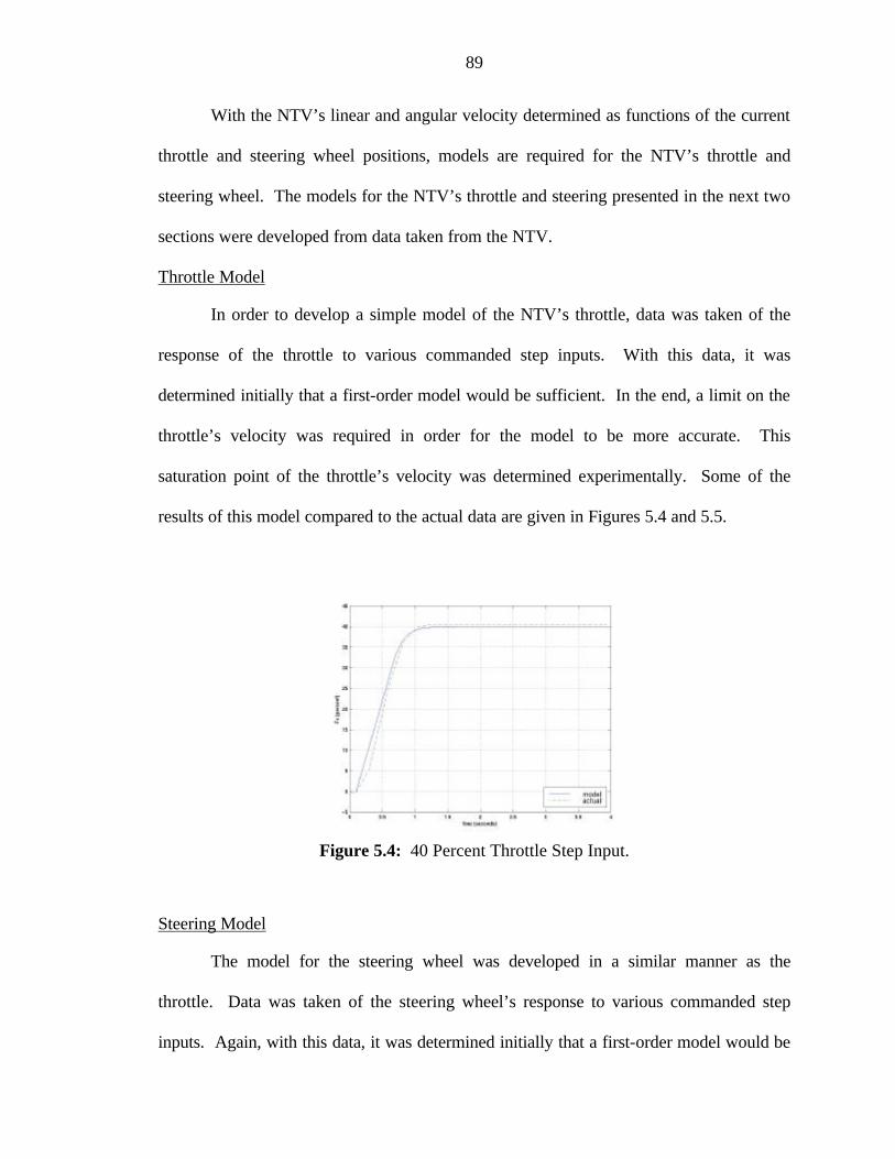
89
With the NTV’s linear and angular velocity determined as functions of the current
throttle and steering wheel positions, models are required for the NTV’s throttle and
steering wheel. The models for the NTV’s throttle and steering presented in the next two
sections were developed from data taken from the NTV.
Throttle Model
In order to develop a simple model of the NTV’s throttle, data was taken of the
response of the throttle to various commanded step inputs. With this data, it was
determined initially that a first-order model would be sufficient. In the end, a limit on the
throttle’s velocity was required in order for the model to be more accurate. This
saturation point of the throttle’s velocity was determined experimentally. Some of the
results of this model compared to the actual data are given in Figures 5.4 and 5.5.
Figure 5.4: 40 Percent Throttle Step Input.
Steering Model
The model for the steering wheel was developed in a similar manner as the
throttle. Data was taken of the steering wheel’s response to various commanded step
inputs. Again, with this data, it was determined initially that a first-order model would be

90
sufficient with a limit on the steering wheel’s velocity. But, a limit on the steering
wheel’s acceleration was required also in order for the model to be more accurate. Both
of these saturation points of the steering wheel’s velocity and acceleration were
determined experimentally. Some of the results of this model compared to the actual data
are given in Figures 5.6 and 5.7.
Figure 5.5: 100 Percent Throttle Step Input.
Figure 5.6: 40 Percent Steering Step Input.

91
Figure 5.7: 100 Percent Steering Step Input.
Simulation Results
Three different paths are used to test the new geometric path-tracking algorithm.
A “U” shape path is used to test going from a straight section into a curve, and from a
curve back into a straight section. A figure eight path is used to test going from a right
curve into a left curve, and from a left curve into a right curve. And finally, a straight
path with a jog in the middle is used to test jumping from a small error in position and
orientation to large errors. For comparison, follow-the-carrot and pure pursuit path-
tracking methods are implemented and tested using the same paths in simulation. In
order to focus on each path-tracking technique’s sensitivity to the look-ahead distance at
various speeds, the constant k for vector pursuit methods 1 and 2 was chosen first through
some initial experiments. The constant was chosen to be 4.0 and 1.5 for methods 1 and 2,
respectively. On account of the large number of tests, the results are shown graphically
in Appendix B.
The first tests, shown in Figures B.1 through B.4, are a “U” shape path with a
tracking speed of 1.5 mps and a look-ahead distance of 3 meters. Each method was

92
capable of navigating this path with relatively small position and heading errors. Next,
using the same path, the look-ahead distance was increased to 5 meters, and the tracking
speed was increased to 3.0 mps for the tests shown in Figure B.5 through B.8. Again,
each method navigated the path with small position and heading errors. The last group of
tests using the “U” shape path is shown in Figures B.9 through B.12. The tracking speed
for these tests was increased to 4.5 mps and the look-ahead distance was increased to 7
meters. Follow-the-carrot path-tracking method was unable to execute this path without
large oscillations coming out of the curved section. The other path-tracking techniques,
pure pursuit and vector pursuit methods 1 and 2, were able to execute the path with small
position and heading errors.
The next path used to test the different path-tracking techniques is a figure eight
path. Just as before, the tracking speed and the look-ahead distance were varied. Figures
B.13 through B.16 show the results of the path-tracking techniques with a tracking speed
of 1.5 mps and a look-ahead distance of 3 meters. Each technique was able to navigate
the path with small position and heading errors. Next, in Figures B.17 through B.20, the
tracking speed was increased to 3.0 mps and the look-ahead distance was increased to 5
meters. Again, all path-tracking techniques tested were able to navigate the path with
relatively small position and heading errors. Figures B.21 through B.24 show the results
of increasing the tracking speed to 4.5 mps and the look-ahead distance to 7 meters. Just
as for the “U” shape path at 4.5 mps, the follow-the-carrot method is no longer able track
the path without large oscillations, while the remaining techniques were able to navigate
the figure eight path with small position and heading errors.
93
Finally, a path with a sudden jog in the middle is used to test the path-tracking
techniques. Initially, the tracking speed is set to 1.5 mps and the look-ahead distance is
set to 3 meters. Each path-tracking technique is tested with the distance of the jog
varying from 2 to 6 meters. These results are shown in Figures B.25 through B.44. Both
the follow-the-carrot and the vector pursuit method 1 resulted in oscillations after the jog.
Both pure pursuit and vector pursuit method 2 are able to navigate the path without
resultant oscillations. It is noticed that the pure pursuit method converges slightly faster
than the vector pursuit method 2. This is characteristic is the result of vector pursuit
method 2 considering the orientation of the look-ahead point as well as the position.
In Figures B.45 through B.64, the tracking speed is set to 3.0 mps now and the
look-ahead distance is set to 5 meters. Similar results are obtained from the follow-the-
carrot method and the vector pursuit method 2 after the jog as was obtained for the slower
tracking speed. Pure pursuit path-tracking technique results in large position errors, but
still no oscillations. Vector pursuit method 2 results in a much smaller position error than
pure pursuit, and also does not exhibit the oscillations, whereas follow-the-carrot and
vector pursuit method 1 do exhibit oscillations.
Finally, the tracking speed is set to 4.5 mps and the look-ahead distance is set to 7
meters. The results of these tests of the paths with a jog in the middle are given in
Figures B.65 through B.84. Again, follow-the-carrot and vector pursuit method 1 result
in large oscillations about the path. Pure pursuit results in some oscillation for the
smaller jogs and large position errors for the larger jogs. Vector pursuit method 2, on the
other hand, results in a very smooth transition from the path before the jog to the path
after the jog.
94
Simulation tests show that vector pursuit method 1 had difficulty handling the test
path with a jog in the middle. It is speculated that the reason for this difficulty is due to
the fact that the vehicle constraints were ignored initially when determining the desired
motion. Because of these results, vector pursuit method 1 is not tested further in
implementation. On the other hand, simulation tests show promising results for the
vector pursuit method 2 path-tracking technique. Therefore, in order to continue testing
this technique, it is implemented on the MCU of the NTV.
Implementation Results
Testing vector pursuit path-tracking method in simulation was done simply to
validate the possibility of this method working on the NTV. Since the models used to
test the path-tracking algorithm in simulation were simple and obviously not exact, the
real test is the actual implementation on the NTV. The simulation tests proved to be
useful since poor results were obtained from vector pursuit method 1 from the tests of a
straight path with a jog in the middle. Again, for this reason, vector pursuit method 1 is
not tested on the NTV.
The same paths used to test vector pursuit in simulation are used to test it on the
NTV. Once more, the constant k of the vector pursuit method 2 is kept at 1.5 in order to
focus on the technique’s sensitivity to the look-ahead distance. The results of vector
pursuit path tracking on the NTV are compared again to follow-the-carrot and pure
pursuit path-tracking techniques, which were implemented on the NTV. Because of the
large number, plots of the planned path and of the actual path measured from the position
system for these tests are shown in Appendix C.
The path used first for testing the path-tracking techniques is a “U” shape path
with 60-meter straight sections and a 15-meter turning radius on the curved section. Each
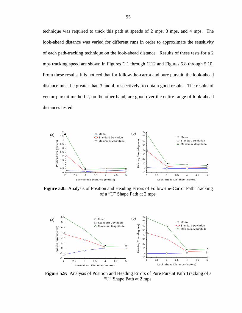
95
technique was required to track this path at speeds of 2 mps, 3 mps, and 4 mps. The
look-ahead distance was varied for different runs in order to approximate the sensitivity
of each path-tracking technique on the look-ahead distance. Results of these tests for a 2
mps tracking speed are shown in Figures C.1 through C.12 and Figures 5.8 through 5.10.
From these results, it is noticed that for follow-the-carrot and pure pursuit, the look-ahead
distance must be greater than 3 and 4, respectively, to obtain good results. The results of
vector pursuit method 2, on the other hand, are good over the entire range of look-ahead
distances tested.
2 2.5 3 3.5 4 4.5 50
0.5
1
1.5
2
2.5
3
3.5
4
4.5
5
Look-ahead Distance (meters)
Pos
ition
Err
or (
met
ers)
MeanStandard DeviationMaximum Magnitude
2 2.5 3 3.5 4 4.5 5-10
0
10
20
30
40
50
60
70
80
Look-ahead Distance (meters)
Hea
ding
Err
or (
degr
ees)
MeanStandard DeviationMaximum Magnitude
(a) (b)
Figure 5.8: Analysis of Position and Heading Errors of Follow-the-Carrot Path Tracking
of a “U” Shape Path at 2 mps.
(a) (b)
2 2.5 3 3.5 4 4.5 5-2
-1
0
1
2
3
4
5
6
Look-ahead Distance (meters)
Pos
ition
Err
or (
met
ers)
MeanStandard DeviationMaximum Magnitude
2 2.5 3 3.5 4 4.5 5-10
0
10
20
30
40
50
60
70
80
Look-ahead Distance (meters)
Hea
ding
Err
or (
degr
ees)
MeanStandard DeviationMaximum Magnitude
Figure 5.9: Analysis of Position and Heading Errors of Pure Pursuit Path Tracking of a
“U” Shape Path at 2 mps.
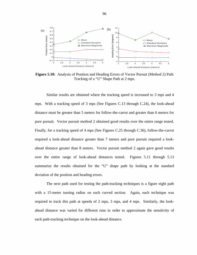
96
(a) (b)
2 2.5 3 3.5 4 4.5 5-0.1
0
0.1
0.2
0.3
0.4
0.5
0.6
0.7
0.8
Look-ahead Distance (meters)
Pos
ition
Err
or (
met
er)
MeanS tandard DeviationMaximum Magnitude
2 2.5 3 3.5 4 4.5 5-2
0
2
4
6
8
10
12
Look-ahead Distance (meters)
Hea
ding
Err
or (
degr
ees)
MeanStandard DeviationMaximum Magnitude
Figure 5.10: Analysis of Position and Heading Errors of Vector Pursuit (Method 2) Path
Tracking of a “U” Shape Path at 2 mps.
Similar results are obtained where the tracking speed is increased to 3 mps and 4
mps. With a tracking speed of 3 mps (See Figures C.13 through C.24), the look-ahead
distance must be greater than 5 meters for follow-the-carrot and greater than 6 meters for
pure pursuit. Vector pursuit method 2 obtained good results over the entire range tested.
Finally, for a tracking speed of 4 mps (See Figures C.25 through C.36), follow-the-carrot
required a look-ahead distance greater than 7 meters and pure pursuit required a look-
ahead distance greater than 8 meters. Vector pursuit method 2 again gave good results
over the entire range of look-ahead distances tested. Figures 5.11 through 5.13
summarize the results obtained for the “U” shape path by looking at the standard
deviation of the position and heading errors.
The next path used for testing the path-tracking techniques is a figure eight path
with a 15-meter turning radius on each curved section. Again, each technique was
required to track this path at speeds of 2 mps, 3 mps, and 4 mps. Similarly, the look-
ahead distance was varied for different runs in order to approximate the sensitivity of
each path-tracking technique on the look-ahead distance.

97
(a) (b)
2 2.5 3 3.5 4 4.5 50
0.5
1
1.5
2
2.5
3
Look-ahead Distance (meters)Pos
ition
Err
or S
tand
ard
Dev
iatio
n (m
eter
s)
Follow The CarrotPure PursuitVector Pursuit
2 2.5 3 3.5 4 4.5 50
5
10
15
20
25
30
35
40
45
Look-ahead Distance (meters)Hea
ding
Err
or S
tand
ard
Dev
iatio
n (d
egre
es)
Follow The CarrotPure PursuitVector Pursuit
Figure 5.11: Standard Deviation of Position and Heading Errors of a “U” shape path at 2
mps.
(a) (b)
4 4.5 5 5.5 6 6.5 70
0.5
1
1.5
2
2.5
3
Look-ahead Distance (meters)Pos
ition
Err
or S
tand
ard
Dev
iatio
n (m
eter
s)
Follow The CarrotPure PursuitVector Pursuit
4 4.5 5 5.5 6 6.5 70
5
10
15
20
25
30
35
40
Look-ahead Distance (meters)Hea
ding
Err
or S
tand
ard
Dev
iatio
n (d
egre
es)
Follow The CarrotPure PursuitVector Pursuit
Figure 5.12: Standard Deviation of Position and Heading Errors of a “U” shape path at 3
mps.
(a) (b)
5 5.5 6 6.5 7 7.5 8 8.5 90
0.5
1
1.5
2
2.5
3
3.5
4
4.5
Look-ahead Distance (meters)Pos
ition
Err
or S
tand
ard
Dev
iatio
n (m
eter
s)
Follow The CarrotPure PursuitVector Pursuit
5 5.5 6 6.5 7 7.5 8 8.5 90
5
10
15
20
25
30
35
40
45
50
Look-ahead Distance (meters)Hea
ding
Err
or S
tand
ard
Dev
iatio
n (d
egre
es)
Follow The CarrotPure PursuitVector Pursuit
Figure 5.13: Standard Deviation of Position and Heading Errors of a “U” shape path at 4
mps.
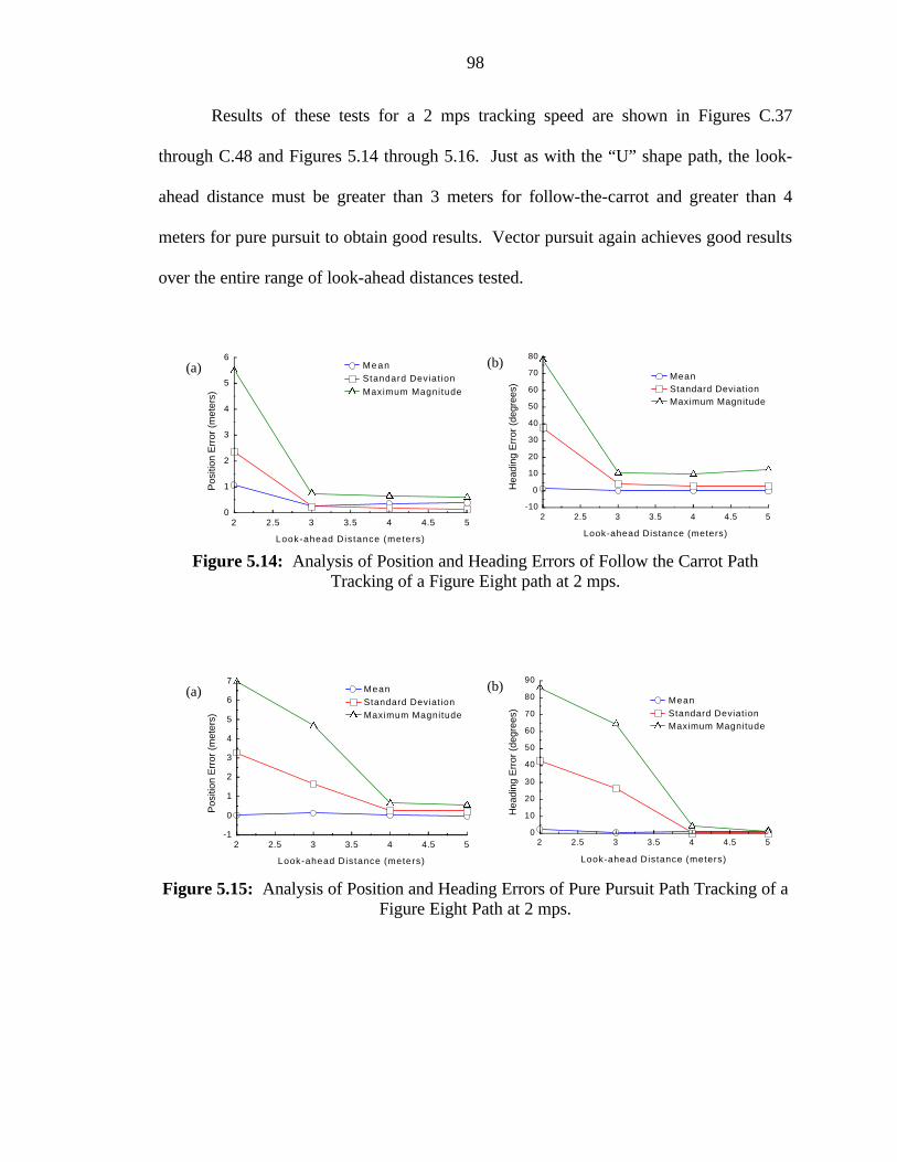
98
Results of these tests for a 2 mps tracking speed are shown in Figures C.37
through C.48 and Figures 5.14 through 5.16. Just as with the “U” shape path, the look-
ahead distance must be greater than 3 meters for follow-the-carrot and greater than 4
meters for pure pursuit to obtain good results. Vector pursuit again achieves good results
over the entire range of look-ahead distances tested.
(a) (b)
2 2.5 3 3.5 4 4.5 50
1
2
3
4
5
6
Look-ahead Distance (meters)
Pos
ition
Err
or (
met
ers)
MeanStandard Deviat ion
Maximum Magnitude
2 2.5 3 3.5 4 4.5 5-10
0
10
20
30
40
50
60
70
80
Look-ahead Distance (meters)
Hea
ding
Err
or (
degr
ees)
MeanStandard DeviationMaximum Magnitude
Figure 5.14: Analysis of Position and Heading Errors of Follow the Carrot Path
Tracking of a Figure Eight path at 2 mps.
(a) (b)
2 2.5 3 3.5 4 4.5 5-1
0
1
2
3
4
5
6
7
Look-ahead Distance (meters)
Pos
ition
Err
or (
met
ers)
MeanStandard DeviationMaximum Magnitude
2 2.5 3 3.5 4 4.5 50
10
20
30
40
50
60
70
80
90
Look-ahead Distance (meters)
Hea
ding
Err
or (
degr
ees)
MeanStandard DeviationMaximum Magnitude
Figure 5.15: Analysis of Position and Heading Errors of Pure Pursuit Path Tracking of a
Figure Eight Path at 2 mps.

99
(a) (b)
2 2.5 3 3.5 4 4.5 5
0
0.5
1
1.5
2
Look-ahead Distance (meters)
Pos
ition
Err
or (
met
ers)
MeanStandard DeviationMaximum Magnitude
2 2.5 3 3.5 4 4.5 50
5
10
15
20
25
30
Look-ahead Distance (meters)
Hea
ding
Err
or (
degr
ees)
MeanStandard DeviationMaximum Magnitude
Figure 5.16: Analysis of Position and Heading Errors of Vector Pursuit (Method 2) Path
Tracking of a “U” Shape Path at 2 mps.
As expected, similar results are obtained for the figure eight path as for the “U”
shape path where the tracking speed is increased to 3 mps and 4 mps. With a tracking
speed of 3 mps (See Figures C.49 through C.60), the look-ahead distance must be greater
than 5 meters for follow-the-carrot and greater than 6 meters for pure pursuit. Vector
pursuit method 2 obtained good results over the entire range tested. Finally, for a
tracking speed of 4 mps (See Figures C.61 through C.72), follow-the-carrot required a
look-ahead distance greater than 7 meters and pure pursuit required a look-ahead distance
greater than 8 meters. Vector pursuit method 2 again gave good results over the entire
range of look-ahead distances tested. Figures 5.17 through 5.19 summarize the results
obtained for the figure eight path by looking at the standard deviation of the position and
heading errors for a tracking speed of 2 meters per second. From these figures, it is
obvious that vector pursuit is able to maintain small position and heading errors with
smaller look-ahead distances than both follow-the-carrot and pure pursuit. Decreasing
the look-ahead distance below a certain point results in large errors for both follow-the-
carrot and pure pursuit path-tracking techniques.

100
(a) (b)
2 2.5 3 3.5 4 4.5 50
0.5
1
1.5
2
2.5
3
3.5
Look-ahead Distance (meters)Pos
ition
Err
or S
tand
ard
Dev
iatio
n (m
eter
s)
Follow The CarrotPure PursuitVector Pursuit
2 2.5 3 3.5 4 4.5 50
5
10
15
20
25
30
35
40
45
Look-ahead Distance (meters)Hea
ding
Err
or S
tand
ard
Dev
iatio
n (d
egre
es)
Follow The CarrotPure PursuitVector Pursuit
Figure 5.17: Standard Deviation of Position and Heading Errors of a Figure Eight Path
at 2 mps.
(a) (b)
4 4.5 5 5.5 6 6.5 70
0.5
1
1.5
2
2.5
3
3.5
Look-ahead Distance (meters)Pos
ition
Err
or S
tand
ard
Dev
iatio
n (m
eter
s)
Follow The CarrotPure PursuitVector Pursuit
4 4.5 5 5.5 6 6.5 70
5
10
15
20
25
30
35
40
45
Look-ahead Distance (meters)Hea
ding
Err
or S
tand
ard
Dev
iatio
n (d
egre
es)
Follow The CarrotPure PursuitVector Pursuit
Figure 5.18: Standard Deviation of Position and Heading Errors of a Figure Eight Path
at 3 mps.
(a) (b)
5 5.5 6 6.5 7 7.5 8 8.5 90
0.5
1
1.5
2
2.5
3
3.5
4
4.5
5
Look-ahead Distance (meters)Pos
ition
Err
or S
tand
ard
Dev
iatio
n (m
eter
s)
Follow The CarrotPure PursuitVector Pursuit
5 5.5 6 6.5 7 7.5 8 8.5 90
10
20
30
40
50
60
Look-ahead Distance (meters)Hea
ding
Err
or S
tand
ard
Dev
iatio
n (d
egre
es)
Follow The CarrotPure PursuitVector Pursuit
Figure 5.19: Standard Deviation of Position and Heading Errors of a Figure Eight Path
at 4 mps.
101
By looking at the standard deviation of position and heading errors in Figures
5.11 through 5.13 and Figures 5.17 through 5.19 for each path-tracking method, vector
pursuit shows to be less sensitive to the look-ahead distance, especially for smaller values
of look-ahead distances. This definitely is desirable for the reasons mentioned earlier.
For example, suppose follow-the-carrot path tracking is utilized with a look-ahead
distance of 3 meters and a tracking speed of 2 mps. Good results are obtained under
normal circumstances. But, if the speed were to increase just slightly, e.g., going down a
hill, stability would definitely be a concern. A similar example could be made of pure
pursuit path tracking.
In addition to being concerned about the path-tracking technique’s sensitivity of
the look-ahead distance to various speeds, the sensitivity of the path-tracking technique to
large position and heading errors is also a concern. In order to test this, a straight path is
used with a jog in the middle, where this jog is varied from 2 meters to 6 meters. This is
tested again for follow-the-carrot and pure pursuit path-tracking techniques in addition to
vector pursuit, at tracking speeds of 2, 3, and 4 meters per second. For each speed, a
look-ahead distance is chosen so that all three path-tracking techniques would perform
well with small position and heading errors.
Initially, the desired tracking speed was set to 2 mps with a look-ahead distance of
5 meters. The results of these tests are given in Figures C.73 through C.87. First, it is
noted that all three methods were able to recover after the jog in the path and converge
back to the desired path. Beyond that, it is also noticed that both follow-the-carrot and
pure pursuit result in a larger overshoot of the desired path than vector pursuit. In fact,
for small jogs in the path, vector pursuit has almost no overshoot.
102
Next, the desired tracking speed was set to 3 mps with a look-ahead distance of 7
meters. The results of these tests are given in Figures C.88 through C.102. At this speed
and with this look-ahead distance, follow-the-carrot is no longer able to recover after the
jog in the path but results in oscillations about the path. Both pure pursuit and vector
pursuit are able to converge to the path after the jog. Although, as before, pure pursuit
has a larger overshoot than vector pursuit before converging to the path. Again, vector
pursuit has almost no overshoot for each test.
Finally, the desired tracking speed was set to 4 mps with a look-ahead-distance of
9 meters. This time, however, follow-the-carrot method was not tested for safety reasons.
Large oscillations at that speed could result in the NTV rolling over. So, the results of
pure pursuit and vector pursuit are given in Figures C.103 through C.112. Both pure
pursuit and vector pursuit are able to recover after the jog in the path by converging back
into the desired path.
Navigating the NTV in Reverse
In addition to implementing the vector pursuit path-tracking method for the NTV
going forward, it was implemented also for going backwards. As in the previous tests, a
“U” shape and a figure eight path are used for testing. Figures C.113 through C.115 give
the results of the “U” shape path at 2 mps, 3 mps, and 4 mps, respectively. And, figures
C.116 through C.118 give the results of the figure eight path at 2 mps, 3 mps, and 4 mps,
respectively. Similar results were obtained going backwards as were obtained going
forward.

103
Cybermotion K2A Implementation Results
Cybermotion K2A is a three-wheel synchronous drive robot. Shawver first
automated this robot under an earlier version of the MAX architecture in 1998 [88]. The
variables that are available to control the K2A vehicle are a drive value and a steer value.
The VCU consists of a Little Giant that is used to convert the wrench command to a drive
value and a steer value. Navigation of planned paths was accomplished by using follow-
the-carrot path tracking in conjunction with PID controllers. Oscillation was noted as a
problem when the vehicle attempted to navigate from a curved section to a straight
section of the path. One of the test paths used by Shawver was a “U” shaped path where
the curved section has a turning radius of approximately 1.3 meters. Test results for this
path had an average error of 4 cm and a maximum error of 20 cm.
The total time required to implement vector pursuit and the two FRMLC
controllers on the K2A was less than a day. The MCU was the only module that was
updated, since the Cybermotion K2A was operating already under the MAX architecture.
This was accomplished by simply copying the source code on the NTV’s MCU to the
K2A’s MCU. A short amount of time was used to adjust the look-ahead distance and
constant k tuning parameters. A “U” shape path and a figure eight path were used to test
the navigation with a look-ahead distance of 0.1 meters and the constant k was set to 4.0.
The planned path and the actual path measured by the position system of these two tests
are shown in Figures 5.20 and 5.21. For the “U” shape test path, the average error was 2
cm with a standard deviation of 2 cm and a maximum magnitude of error of 6cm. For the
figure eight path, the average error was –1 cm with a 3 cm standard deviation and a
maximum magnitude of error of 8 cm.
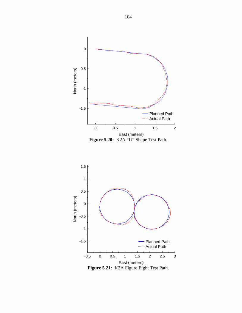
104
0 0.5 1 1.5 2
-1.5
-1
-0.5
0
East (meters)
Nor
th (
met
ers)
Planned PathActual Path
Figure 5.20: K2A “U” Shape Test Path.
-0.5 0 0.5 1 1.5 2 2.5 3
-1.5
-1
-0.5
0
0.5
1
1.5
East (meters)
Nor
th (
met
ers)
Planned PathActual Path
Figure 5.21: K2A Figure Eight Test Path.
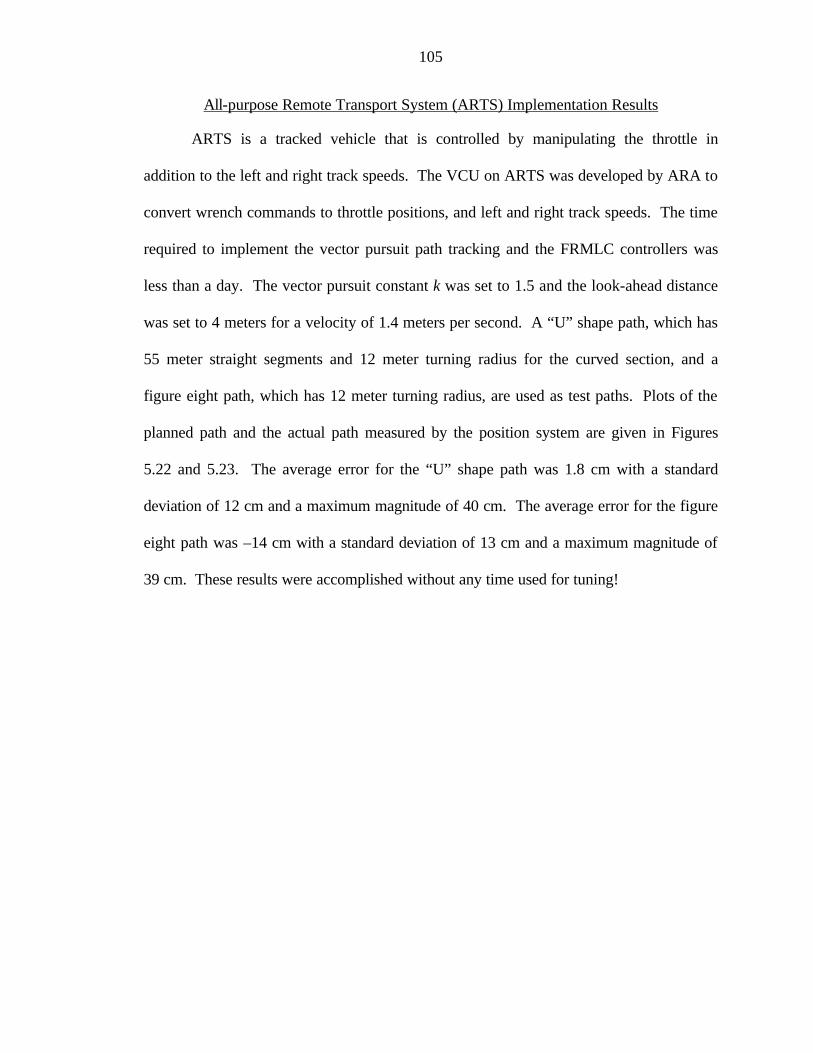
105
All-purpose Remote Transport System (ARTS) Implementation Results
ARTS is a tracked vehicle that is controlled by manipulating the throttle in
addition to the left and right track speeds. The VCU on ARTS was developed by ARA to
convert wrench commands to throttle positions, and left and right track speeds. The time
required to implement the vector pursuit path tracking and the FRMLC controllers was
less than a day. The vector pursuit constant k was set to 1.5 and the look-ahead distance
was set to 4 meters for a velocity of 1.4 meters per second. A “U” shape path, which has
55 meter straight segments and 12 meter turning radius for the curved section, and a
figure eight path, which has 12 meter turning radius, are used as test paths. Plots of the
planned path and the actual path measured by the position system are given in Figures
5.22 and 5.23. The average error for the “U” shape path was 1.8 cm with a standard
deviation of 12 cm and a maximum magnitude of 40 cm. The average error for the figure
eight path was –14 cm with a standard deviation of 13 cm and a maximum magnitude of
39 cm. These results were accomplished without any time used for tuning!
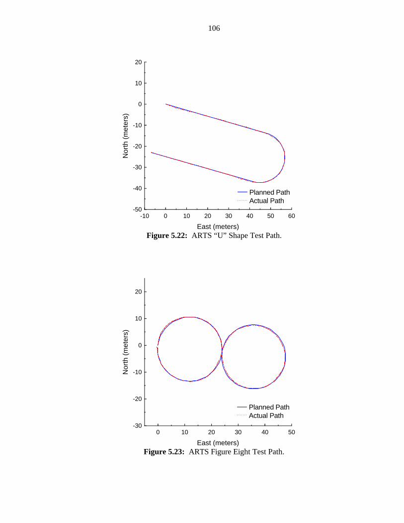
106
-10 0 10 20 30 40 50 60-50
-40
-30
-20
-10
0
10
20
East (meters)
Nor
th (
met
ers)
Planned PathActual Path
Figure 5.22: ARTS “U” Shape Test Path.
0 10 20 30 40 50-30
-20
-10
0
10
20
East (meters)
Nor
th (
met
ers)
Planned PathActual Path
Figure 5.23: ARTS Figure Eight Test Path.

107
CHAPTER 6 CONCLUSIONS AND FUTURE WORK
Conclusions
Current geometric path-tracking methods such as pure pursuit or follow-the-carrot
only use a desired position in order to determine a desired vehicle motion. Proportional
path-tracking method, uses both a desired position and heading, but is geometrically
meaningless by adding terms with different units. Vector pursuit is a new geometric
path-tracking algorithm that takes advantage of a desired orientation as well as a desired
position while remaining geometrically meaningful.
Two methods based on the theory of screws were developed for vector pursuit. In
both methods, a desired instantaneous screw is calculated to represent the motion of the
vehicle from its current position and orientation to a position and orientation on the path.
The first method initially ignores the vehicle constraints when determining this desired
instantaneous screw, and then deals with them afterward. The second method considers
the constraints in determining the desired instantaneous screw. Both methods are used to
determine a desired vehicle turning rate.
A fuzzy reference model learning controller (FRMLC) was implemented to track
the desired vehicle turning rate. This controller was designed from parameters of known
vehicle characteristics such as the maximum turning rate and the maximum speed.
Assuming that the user would set the desired tracking speed, a second FRMLC was
implemented to track this desired speed. Again, this controller was designed from

108
parameters of known vehicle characteristics such as the maximum speed and the
maximum allowable pitch.
Both vector pursuit path-tracking methods were tested in simulation and
compared to both follow-the-carrot and pure pursuit path-tracking methods. In these
tests, it was determined that the first method, for determining the desired instantaneous
screw, had difficulty handling large position and heading errors. The second method for
determining the instantaneous screw, on the other hand, showed to be promising in
simulation.
Then, this method was implemented on the Navigation Test Vehicle (NTV),
which was designed and built by the Center for Intelligent Machines and Robotics
(CIMAR) at the University of Florida. It was tested on various paths and again compared
to follow-the-carrot and pure pursuit path-tracking techniques. Through these tests,
vector pursuit proved to be more robust. Vector pursuit was less sensitive to the chosen
look-ahead distance at various speeds, and it was able to handle situations where large
position and orientation errors could occur, e.g., after an unexpected obstacle was
encountered.
In addition to implementing the vector pursuit path tracking and the FRMLCs on
the NTV, they were implemented also on a Cybermotion K2A and on an All-purpose
Remote Transport System. In each case, the time required to implement the path tracking
and controllers required less than a day.
Future Work
The first method used in vector pursuit to calculate the desired instantaneous
screw did not work out for the NTV becaues of large oscillations when tested with a path
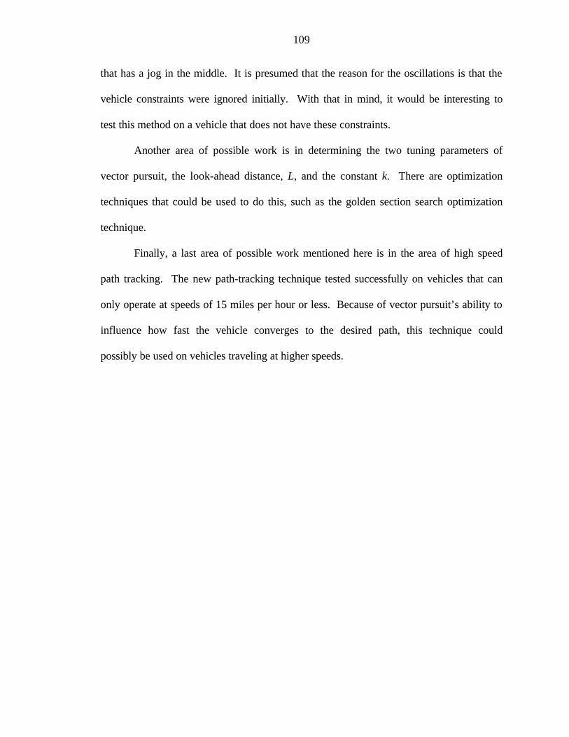
109
that has a jog in the middle. It is presumed that the reason for the oscillations is that the
vehicle constraints were ignored initially. With that in mind, it would be interesting to
test this method on a vehicle that does not have these constraints.
Another area of possible work is in determining the two tuning parameters of
vector pursuit, the look-ahead distance, L, and the constant k. There are optimization
techniques that could be used to do this, such as the golden section search optimization
technique.
Finally, a last area of possible work mentioned here is in the area of high speed
path tracking. The new path-tracking technique tested successfully on vehicles that can
only operate at speeds of 15 miles per hour or less. Because of vector pursuit’s ability to
influence how fast the vehicle converges to the desired path, this technique could
possibly be used on vehicles traveling at higher speeds.
110
APPENDIX A MAX INTERFACE SPECIFICATION FOR UNMANNED VEHICLES
Developed by the Center for Intelligent Machines and Robotics at the University of Florida under the sponsorship of the
Air Force Research Laboratory, Tyndall Air Force Base, Florida

111
1.0 Introduction...........................................................................................................113
2.0 Standardized Message Format (ASCII)..................................................................115
2.1 Vehicle Control Unit (VCU) (ASCII) ....................................................................119
VCU Start Report ....................................................................................................120 VCU Stop Report ....................................................................................................121 VCU Shutdown .......................................................................................................122 VCU Reinitialize .....................................................................................................123 VCU Standby ..........................................................................................................124 VCU Request Configuration....................................................................................125 VCU Request Status ................................................................................................126 VCU Propulsive Wrench .........................................................................................127 VCU Resistive Wrench............................................................................................128 VCU Report ............................................................................................................129 VCU Configuration Report......................................................................................131 VCU Status Report ..................................................................................................132
2.2 Position Systems (POS) (ASCII) ...........................................................................133
POS Start Report .....................................................................................................134 POS Stop Report .....................................................................................................135 POS Shutdown ........................................................................................................136 POS Reinitialize ......................................................................................................137 POS Standby ...........................................................................................................138 POS Set Configuration ............................................................................................139 POS Request Configuration.....................................................................................141 POS Request Status .................................................................................................142 POS Report .............................................................................................................143 POS Configuration Report.......................................................................................146 POS Status Report ...................................................................................................148
2.3 Mobility Control Unit (MCU) (ASCII) ..................................................................149
MCU Start Report ...................................................................................................151 MCU Stop Report....................................................................................................152 MCU Shutdown.......................................................................................................153 MCU Reinitialize ....................................................................................................154 MCU Standby..........................................................................................................155 MCU Set Configuration...........................................................................................156

112
MCU Request Configuration ...................................................................................157 MCU Request Status ...............................................................................................158 MCU Execute Path..................................................................................................159 MCU Pause .............................................................................................................160 MCU Continue ........................................................................................................161 MCU Set Mode .......................................................................................................162 MCU Report............................................................................................................163 MCU Configuration Report .....................................................................................165 MCU Status Report .................................................................................................166
2.4 Detection Mapping Systems (DMS) (ASCII) .........................................................167
DMS Start Report....................................................................................................168 DMS Stop Report ....................................................................................................169 DMS Shutdown.......................................................................................................170 DMS Reinitialize.....................................................................................................171 DMS Standby..........................................................................................................172 DMS Set Configuration ...........................................................................................173 DMS Request Configuration....................................................................................175 DMS Request Status................................................................................................176 DMS Report ............................................................................................................177 DMS Configuration Report......................................................................................180 DMS Status Report..................................................................................................182
2.5 Path Planner (PLN) (ASCII) ..................................................................................183
PLN Shutdown........................................................................................................184 PLN Reinitialize......................................................................................................185 PLN Standby ...........................................................................................................186 PLN Set Configuration ............................................................................................187 PLN Request Configuration.....................................................................................188 PLN Request Status.................................................................................................189 PLN Request Path ...................................................................................................190 PLN Path Report .....................................................................................................192 PLN Configuration Report.......................................................................................194 PLN Status Report...................................................................................................195

113
1.0 Introduction
The Center for Intelligent Machines and Robotics (CIMAR), at the University of Florida, has worked under the guidance of the Air Force Research Laboratory, Tyndall Air Force Base, Florida to develop a series of autonomously navigating vehicles. A Kawasaki Mule 500 all-terrain vehicle named the Mule was first modified for computer control in 1991 for the purpose of providing a test and development platform. The technology developed on this platform has since been applied to a John Deere excavator, an Autonomous Survey Vehicle, and the Joint Amphibious Mine Countermeasures dozer. The original vehicle control architecture was primarily based on a shared memory (blackboard) approach, implemented through the use of multiple 68030 CPU boards running on a VME backplane. The use of shared memory provided the advantage of running critical real-time procedures in parallel and having their resultant data available to all other programs immediately via the VME backplane. This is the key advantage of using shared memory. The problem with shared memory is that it tightly couples all of the sub-systems in an indirect way, making programming errors in the system difficult to trace. The shared or common memory area becomes unmanageable in that a piece of data can be over written in error with impact somewhere else in the system. The result is a system that becomes difficult to maintain or upgrade as new features and hardware are added. In addition, the integration of all the systems into one backplane makes it difficult to use any one sub-system on a different project. For example, to apply the position system to another autonomous vehicle would most certainty require significant changes to both hardware and software. From the experience gathered over the past years of work, a list of four architecture design requirements has emerged. The architecture should:
1. be comprised of a set of well-defined, self-contained, hardware independent modules where only the modules interface is rigorously defined.
2. have the ability to scale up a system’s functionality with different combinations of modules
3. provide a stepping stone toward the development of a standard architecture
The focus of this document is to present a modular architecture that addresses the above design considerations. Detailed information will be provided to document the hardware and software interfaces for a series of independent modules. These modules can then be combined together in order to attain an autonomous navigation capability. Figures A.1 and A.2 provide an overview of the remote system.

114
OperatorControl
Unit
MobilityData
CollectionRSTA
MissionSpecific
Sub-system
Task Level Control
Figure A.1: Architecture Overview.
Autonomous Control Unit
Position System
Detection &MappingSystem
VehicleControlUnit
OperatorControl Unit
PathPlanner
Mobility Control Unit
Operator Control Unit
Position System
Detection & Mapping System
Path PlannerVehicle
Control Unit
Figure A.2: Detail of Mobility.
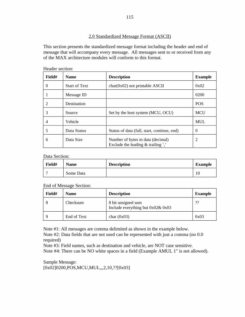
115
2.0 Standardized Message Format (ASCII)
This section presents the standardized message format including the header and end of message that will accompany every message. All messages sent to or received from any of the MAX architecture modules will conform to this format. Header section:
Field#
Name
Description
Example
0
Start of Text
char(0x02) not printable ASCII
0x02
1
Message ID
0200
2
Destination
POS
3
Source
Set by the host system (MCU, OCU)
MCU
4
Vehicle
MUL
5
Data Status
Status of data (full, start, continue, end)
0
6
Data Size
Number of bytes in data (decimal) Exclude the leading & trailing ‘,’
2
Data Section:
Field#
Name
Description
Example
7
Some Data
10
End of Message Section:
Field#
Name
Description
Example
8
Checksum
8 bit unsigned sum Include everything but 0x02& 0x03
??
9
End of Text
char (0x03)
0x03
Note #1: All messages are comma delimited as shown in the example below. Note #2: Data fields that are not used can be represented with just a comma (no 0.0 required) Note #3: Field names, such as destination and vehicle, are NOT case sensitive. Note #4: There can be NO white spaces in a field (Example AMUL 1" is not allowed). Sample Message: [0x02]0200,POS,MCU,MUL,,,2,10,??[0x03]

116
1. Start of text The start of text will be marked by the byte 0x02 2. Message Identification (ID) The message ID identifies a unique message. MAX Modules are assigned a range of message IDs to implement their messaging. The range of message IDs for the Max Modules are defined as follows: Vehicle Control Unit VCU 0x0100 - 0x01ff Position System POS 0x0200 - 0x02ff. Mobility Control Unit MCU 0x0300 - 0x03ff Detection Mapping System DMS 0x0400 - 0x04ff Path Planner PLN 0x0500 - 0x05ff 3. Destination Destination identifies the intended recipient of the message. If the message is a response to a request, then destination identifies the requesting module. 4. Source Source identifies the module that sent the message. 5. Vehicle Vehicle identifies the system that the module is contained in. 6. Data Status Data Status indicates the state of the data. Large data is broken into smaller packets and then transmitted in separate messages. The state of the data can take the form of: FULL_DATA (0) The message sent contains a full data set. START_DATA (1) The message is longer than the maximum, and is therefore broken
into smaller packets. This signifies the start of the packets. CONTINUE_DATA (2) This signifies the continuation of the data. END_DATA (3) This signifies the last data packet of the message. 7. Data Size Data Size gives the size, in bytes, of the data. 8. Data The data content and format is specified in each MAX modules interface document. 9. Checksum Checksum is the 8-bit unsigned sum of all bytes comprising the message packet not including the start of text and the end of text. Includes the comma prior to the checksum. The checksum is also represented in ASCII (2 bytes). 10. End of Text The end of text will be the byte 0x03 Notes: 1. In the data field, sending only the comma where data is not available is allowed. Ex. 1.2,,2, ... 2. All fields in the header must be filled.
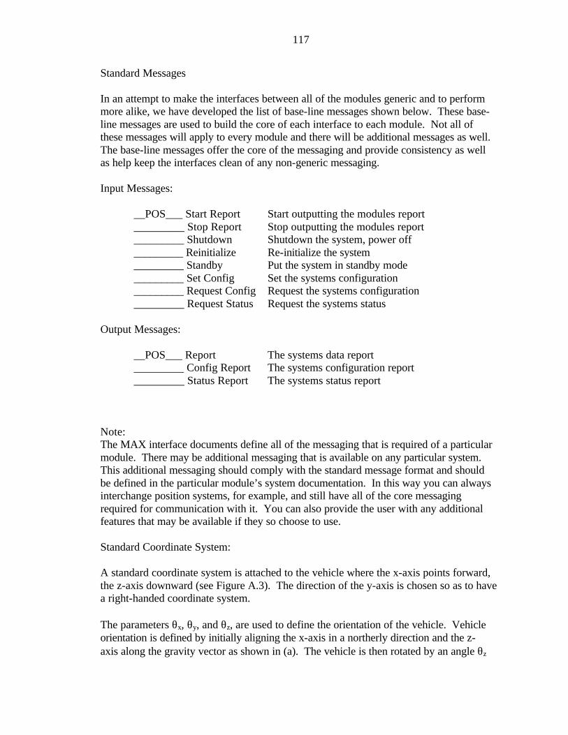
117
Standard Messages In an attempt to make the interfaces between all of the modules generic and to perform more alike, we have developed the list of base-line messages shown below. These base-line messages are used to build the core of each interface to each module. Not all of these messages will apply to every module and there will be additional messages as well. The base-line messages offer the core of the messaging and provide consistency as well as help keep the interfaces clean of any non-generic messaging. Input Messages:
__POS___ Start Report Start outputting the modules report _________ Stop Report Stop outputting the modules report _________ Shutdown Shutdown the system, power off _________ Reinitialize Re-initialize the system _________ Standby Put the system in standby mode _________ Set Config Set the systems configuration _________ Request Config Request the systems configuration _________ Request Status Request the systems status
Output Messages:
__POS___ Report The systems data report _________ Config Report The systems configuration report _________ Status Report The systems status report
Note: The MAX interface documents define all of the messaging that is required of a particular module. There may be additional messaging that is available on any particular system. This additional messaging should comply with the standard message format and should be defined in the particular module’s system documentation. In this way you can always interchange position systems, for example, and still have all of the core messaging required for communication with it. You can also provide the user with any additional features that may be available if they so choose to use. Standard Coordinate System: A standard coordinate system is attached to the vehicle where the x-axis points forward, the z-axis downward (see Figure A.3). The direction of the y-axis is chosen so as to have a right-handed coordinate system. The parameters θx, θy, and θz, are used to define the orientation of the vehicle. Vehicle orientation is defined by initially aligning the x-axis in a northerly direction and the z-axis along the gravity vector as shown in (a). The vehicle is then rotated by an angle θz
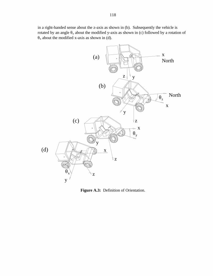
118
in a right-handed sense about the z-axis as shown in (b). Subsequently the vehicle is rotated by an angle θy about the modified y-axis as shown in (c) followed by a rotation of θx about the modified x-axis as shown in (d).
xNorth
yz
North
xy
z
θz
y
z
xθy
x
yzθx
(a)
(b)
(c)
(d)
Figure A.3: Definition of Orientation.
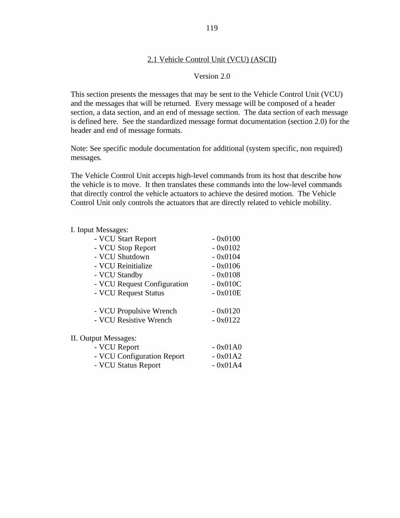
119
2.1 Vehicle Control Unit (VCU) (ASCII)
Version 2.0 This section presents the messages that may be sent to the Vehicle Control Unit (VCU) and the messages that will be returned. Every message will be composed of a header section, a data section, and an end of message section. The data section of each message is defined here. See the standardized message format documentation (section 2.0) for the header and end of message formats. Note: See specific module documentation for additional (system specific, non required) messages. The Vehicle Control Unit accepts high-level commands from its host that describe how the vehicle is to move. It then translates these commands into the low-level commands that directly control the vehicle actuators to achieve the desired motion. The Vehicle Control Unit only controls the actuators that are directly related to vehicle mobility. I. Input Messages:
- VCU Start Report - 0x0100 - VCU Stop Report - 0x0102 - VCU Shutdown - 0x0104 - VCU Reinitialize - 0x0106 - VCU Standby - 0x0108 - VCU Request Configuration - 0x010C - VCU Request Status - 0x010E
- VCU Propulsive Wrench - 0x0120 - VCU Resistive Wrench - 0x0122
II. Output Messages:
- VCU Report - 0x01A0 - VCU Configuration Report - 0x01A2 - VCU Status Report - 0x01A4
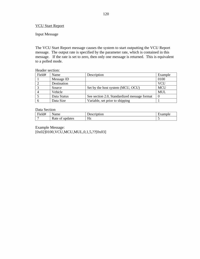
120
VCU Start Report
Input Message The VCU Start Report message causes the system to start outputting the VCU Report message. The output rate is specified by the parameter rate, which is contained in this message. If the rate is set to zero, then only one message is returned. This is equivalent to a polled mode. Header section: Field# Name Description Example 1 Message ID 0100 2 Destination VCU 3 Source Set by the host system (MCU, OCU) MCU 4 Vehicle MUL 5 Data Status See section 2.0, Standardized message format 0 6 Data Size Variable, set prior to shipping 1
Data Section
Field# Name Description Example 7 Rate of updates Hz 5
Example Message: [0x02]0100,VCU,MCU,MUL,0,1,5,??[0x03]
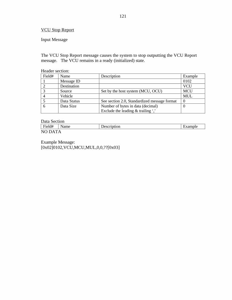
121
VCU Stop Report
Input Message The VCU Stop Report message causes the system to stop outputting the VCU Report message. The VCU remains in a ready (initialized) state. Header section: Field# Name Description Example 1 Message ID 0102 2 Destination VCU 3 Source Set by the host system (MCU, OCU) MCU 4 Vehicle MUL 5 Data Status See section 2.0, Standardized message format 0 6 Data Size Number of bytes in data (decimal)
Exclude the leading & trailing ‘,’ 0
Data Section
Field# Name Description Example NO DATA Example Message: [0x02]0102,VCU,MCU,MUL,0,0,??[0x03]
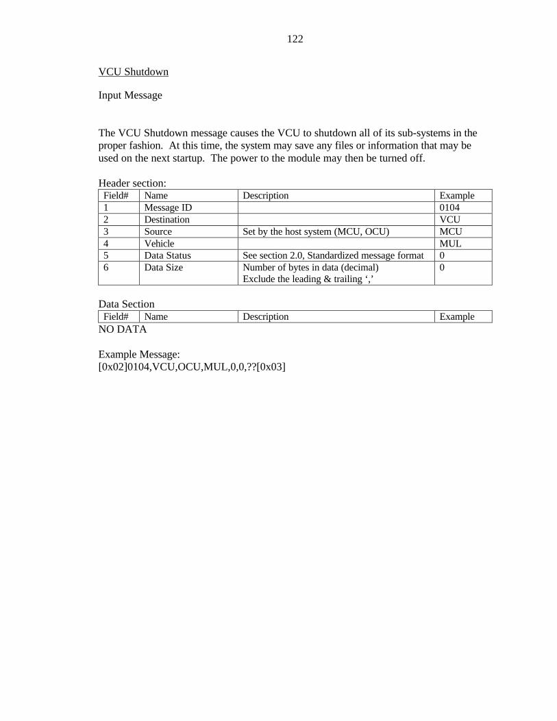
122
VCU Shutdown
Input Message The VCU Shutdown message causes the VCU to shutdown all of its sub-systems in the proper fashion. At this time, the system may save any files or information that may be used on the next startup. The power to the module may then be turned off. Header section: Field# Name Description Example 1 Message ID 0104 2 Destination VCU 3 Source Set by the host system (MCU, OCU) MCU 4 Vehicle MUL 5 Data Status See section 2.0, Standardized message format 0 6 Data Size Number of bytes in data (decimal)
Exclude the leading & trailing ‘,’ 0
Data Section
Field# Name Description Example NO DATA Example Message: [0x02]0104,VCU,OCU,MUL,0,0,??[0x03]

123
VCU Reinitialize
Input Message Commands the VCU to reinitialize each sub-system in the proper sequence to bring the system up to a state of readiness. Once initialized, the VCU will execute commands that cause or resist vehicle motion. The VCU must be initialized for vehicle motion to occur. Header section: Field# Name Description Example 1 Message ID 0106 2 Destination VCU 3 Source Set by the host system (MCU, OCU) MCU 4 Vehicle MUL 5 Data Status See section 2.0, Standardized message format 0 6 Data Size Number of bytes in data (decimal)
Exclude the leading & trailing ‘,’ 0
Data Section
Field# Name Description Example NO DATA Example Message: [0x02]0106,VCU,MCU,MUL,0,0,??[0x03]

124
VCU Standby
Input Message The VCU Standby message causes the system to go into a standby mode. In standby mode the system is alive and ready to be re-initialized. Note: A VCU Shutdown should be given prior to turning system power off. Header section: Field# Name Description Example 1 Message ID 0108 2 Destination VCU 3 Source Set by the host system (MCU, OCU) MCU 4 Vehicle MUL 5 Data Status See section 2.0, Standardized message format 0 6 Data Size Number of bytes in data (decimal)
Exclude the leading & trailing ‘,’ 0
Data Section
Field# Name Description Example NO DATA Example Message: [0x02]0108,VCU,MCU,MUL,0,0,??[0x03]

125
VCU Request Configuration
Input Message This message is used to request the current configuration of the VCU. See VCU Configuration Report for the response definition. Header section: Field# Name Description Example 1 Message ID 010C 2 Destination VCU 3 Source Set by the host system (MCU, OCU) MCU 4 Vehicle MUL 5 Data Status See section 2.0, Standardized message format 0 6 Data Size Number of bytes in data (decimal)
Exclude the leading & trailing ‘,’ 0
Data Section
Field# Name Description Example NO DATA Example Message: [0x02]010C,VCU,MCU,MUL,0,0,?? [0x03]

126
VCU Request Status
Input Message This message is used to request the current status of the VCU. See VCU Status Report for the response definition. Header section: Field# Name Description Example 1 Message ID 010E 2 Destination VCU 3 Source Set by the host system (MCU, OCU) MCU 4 Vehicle MUL 5 Data Status See section 2.0, Standardized message format 0 6 Data Size Number of bytes in data (decimal)
Exclude the leading & trailing ‘,’ 0
Data Section
Field# Name Description Example NO DATA Example Message: [0x02]010E,VCU,MCU,MUL,0,0,??[0x03]
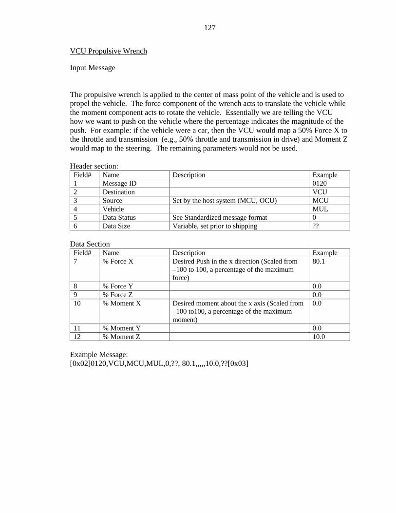
127
VCU Propulsive Wrench
Input Message The propulsive wrench is applied to the center of mass point of the vehicle and is used to propel the vehicle. The force component of the wrench acts to translate the vehicle while the moment component acts to rotate the vehicle. Essentially we are telling the VCU how we want to push on the vehicle where the percentage indicates the magnitude of the push. For example: if the vehicle were a car, then the VCU would map a 50% Force X to the throttle and transmission (e.g., 50% throttle and transmission in drive) and Moment Z would map to the steering. The remaining parameters would not be used. Header section: Field# Name Description Example 1 Message ID 0120 2 Destination VCU 3 Source Set by the host system (MCU, OCU) MCU 4 Vehicle MUL 5 Data Status See Standardized message format 0 6 Data Size Variable, set prior to shipping ??
Data Section
Field# Name Description Example 7 % Force X Desired Push in the x direction (Scaled from
–100 to 100, a percentage of the maximum force)
80.1
8 % Force Y 0.0 9 % Force Z 0.0 10 % Moment X Desired moment about the x axis (Scaled from
–100 to100, a percentage of the maximum moment)
0.0
11 % Moment Y 0.0 12 % Moment Z 10.0
Example Message: [0x02]0120,VCU,MCU,MUL,0,??, 80.1,,,,,10.0,??[0x03]

128
VCU Resistive Wrench
Input Message The resistive wrench is applied to the center of mass point of the vehicle and is used to impede vehicle motion. The resistive wrench uses the same six parameters as the propulsive wrench. For example, if the vehicle were a car, then a 20% Force X command would map to the brake (e.g., brake depressed 20%). Header section: Field# Name Description Example 1 Message ID 0120 2 Destination VCU 3 Source Set by the host system (MCU, OCU) MCU 4 Vehicle MUL 5 Data Status See Standardized message format 0 6 Data Size Variable, set prior to shipping ??
Data Section
Field# Name Description Example 7 % Force X Desired resistive force in the x direction
(Scaled from 0 to100, a percentage of the maximum force)
20.3
8 % Force Y 0.0 9 % Force Z 0.0 10 % Moment X Desired resistive moment about the x axis
(Scaled from 0 to100, a percentage of the maximum moment)
0.0
11 % Moment Y 0.0 12 % Moment Z 0.0
Example Message: [0x02]0120,VCU,MCU,MUL,0,??, 20.3,,,,,,??[0x03]
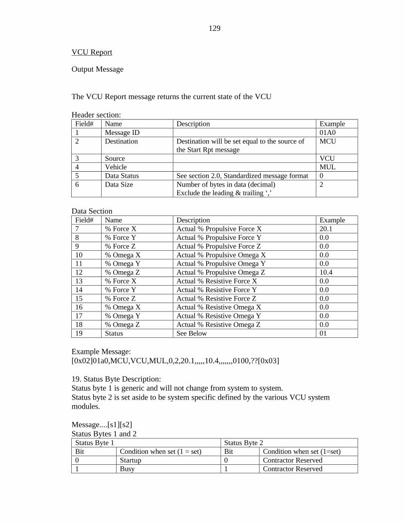
129
VCU Report
Output Message The VCU Report message returns the current state of the VCU Header section: Field# Name Description Example 1 Message ID 01A0 2 Destination Destination will be set equal to the source of
the Start Rpt message MCU
3 Source VCU 4 Vehicle MUL 5 Data Status See section 2.0, Standardized message format 0 6 Data Size Number of bytes in data (decimal)
Exclude the leading & trailing ‘,’ 2
Data Section
Field# Name Description Example 7 % Force X Actual % Propulsive Force X 20.1 8 % Force Y Actual % Propulsive Force Y 0.0 9 % Force Z Actual % Propulsive Force Z 0.0 10 % Omega X Actual % Propulsive Omega X 0.0 11 % Omega Y Actual % Propulsive Omega Y 0.0 12 % Omega Z Actual % Propulsive Omega Z 10.4 13 % Force X Actual % Resistive Force X 0.0 14 % Force Y Actual % Resistive Force Y 0.0 15 % Force Z Actual % Resistive Force Z 0.0 16 % Omega X Actual % Resistive Omega X 0.0 17 % Omega Y Actual % Resistive Omega Y 0.0 18 % Omega Z Actual % Resistive Omega Z 0.0 19 Status See Below 01
Example Message: [0x02]01a0,MCU,VCU,MUL,0,2,20.1,,,,,10.4,,,,,,,0100,??[0x03] 19. Status Byte Description: Status byte 1 is generic and will not change from system to system. Status byte 2 is set aside to be system specific defined by the various VCU system modules. Message....[s1][s2] Status Bytes 1 and 2 Status Byte 1 Status Byte 2 Bit Condition when set (1 = set) Bit Condition when set (1=set) 0 Startup 0 Contractor Reserved 1 Busy 1 Contractor Reserved
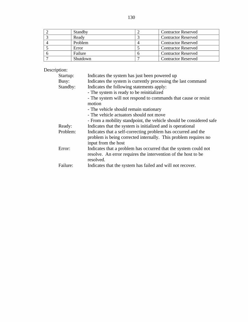
130
2 Standby 2 Contractor Reserved 3 Ready 3 Contractor Reserved 4 Problem 4 Contractor Reserved 5 Error 5 Contractor Reserved 6 Failure 6 Contractor Reserved 7 Shutdown 7 Contractor Reserved
Description:
Startup: Indicates the system has just been powered up Busy: Indicates the system is currently processing the last command Standby: Indicates the following statements apply:
- The system is ready to be reinitialized - The system will not respond to commands that cause or resist motion - The vehicle should remain stationary - The vehicle actuators should not move - From a mobility standpoint, the vehicle should be considered safe
Ready: Indicates that the system is initialized and is operational Problem: Indicates that a self-correcting problem has occurred and the
problem is being corrected internally. This problem requires no input from the host
Error: Indicates that a problem has occurred that the system could not resolve. An error requires the intervention of the host to be resolved.
Failure: Indicates that the system has failed and will not recover.

131
VCU Configuration Report
Output Message This message is used to report the current configuration of the VCU. The following is a description of the parameters: Header section: Field# Name Description Example 1 Message ID 01A2 2 Destination Destination will be set equal to the source of
the Start Rpt message MCU
3 Source VCU 4 Vehicle MUL 5 Data Status See section 2.0, Standardized message format 0 6 Data Size Variable, set prior to shipping ??
Data Section
Field# Name Description Example 7 Text Description Free form text description. May list the main
components used by the system and or other pertinent information.
VCU System: PC/104:
8 System Identification Gives a hex number assigned to the particular VCU so that it may be more uniquely described.
??
9 Vehicle Length Length of the vehicle (Meters) 2.0 10 Vehicle Width Width of the vehicle (Meters) 1.5 11 Vehicle Height Height of the vehicle (Meters) 2.0 12 Turning radius Vehicles minimum turning radius (Meters)
Note: If the vehicle is omnidirectional then this variable should be set to zero.
3.0
13 Max speed X Meters/sec 10.0 14 Max Speed Y Meters/sec 0.0 15 Max Speed Z Meters/sec 0.0 16 Max speed -X Meters/sec 10.0 17 Max Speed -Y Meters/sec 0.0 18 Max Speed -Z Meters/sec 0.0 17 Max Omega X rad/sec 0.0 19 Max Omega Y rad/sec 0.0 20 Max Omega Z rad/sec 0.08 21 Max Theta X Point of static roll over 40.0 22 Max Theta Y Point of static pitch over 50.0
Example Message: [0x02]01A2,MCU,VCU,MUL,0,??,VCU System PC/104, ??,2.1,1.5,2.0,3.0,10.0,,,10.0,,,,,0.08,40.0,50.0??[0x03]
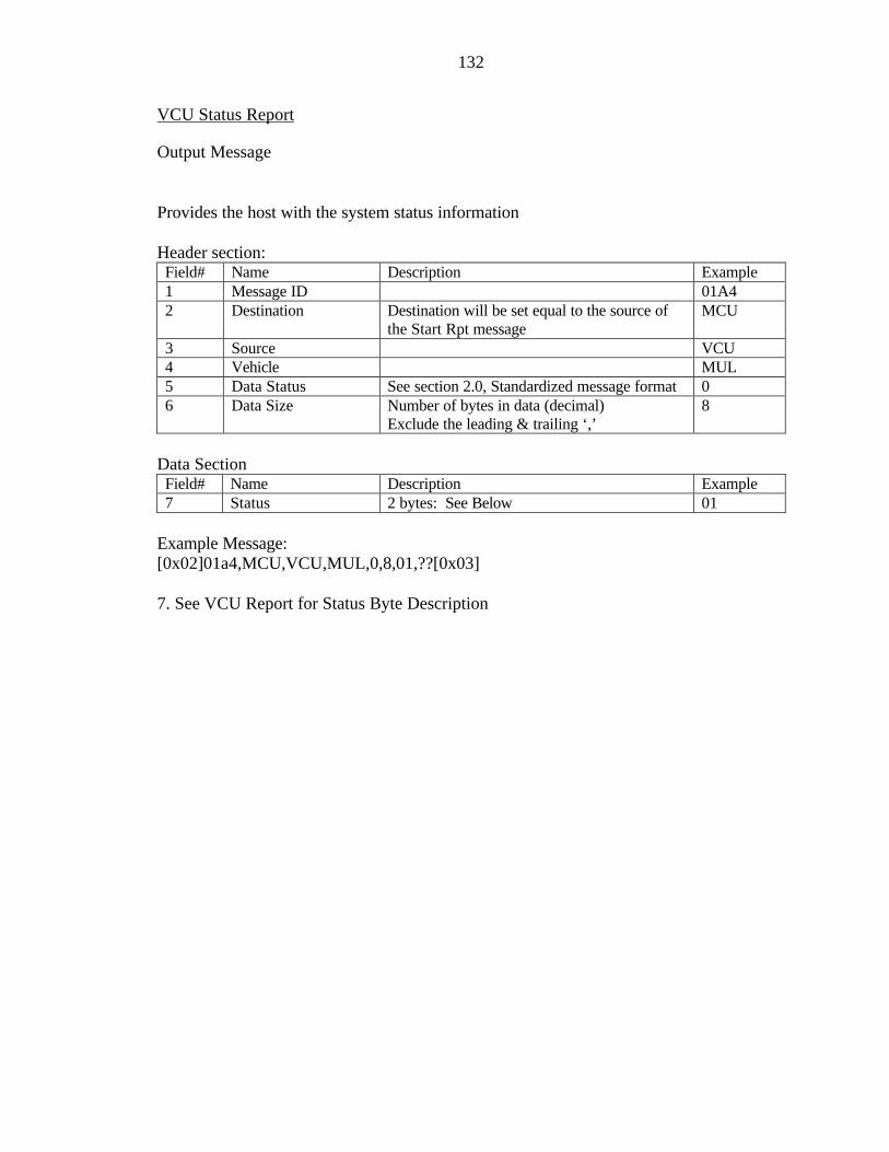
132
VCU Status Report
Output Message Provides the host with the system status information Header section: Field# Name Description Example 1 Message ID 01A4 2 Destination Destination will be set equal to the source of
the Start Rpt message MCU
3 Source VCU 4 Vehicle MUL 5 Data Status See section 2.0, Standardized message format 0 6 Data Size Number of bytes in data (decimal)
Exclude the leading & trailing ‘,’ 8
Data Section
Field# Name Description Example 7 Status 2 bytes: See Below 01
Example Message: [0x02]01a4,MCU,VCU,MUL,0,8,01,??[0x03] 7. See VCU Report for Status Byte Description
133
2.2 Position Systems (POS) (ASCII)
Version 2.0 This section presents the messages that may be sent to the position system and the messages that will be returned. Every message will be composed of a header section, a data section, and an end of message section. The data section of each message is defined here. See the standardized message format documentation (section 2.0) for the header and end of message formats. Note: See specific module documentation for additional (system specific, non required) messages. I. Input Messages:
- POS Start Report - 0x0200 - POS Stop Report - 0x0202 - POS Shutdown - 0x0204 - POS Reinitialize - 0x0206 - POS Standby - 0x0208 - POS Set Configuration - 0x020A - POS Request Configuration - 0x020C - POS Request Status - 0x020E
II. Output Messages:
- POS Report - 0x02A0 - POS Configuration Report - 0x02A2 - POS Status Report - 0x02A4

134
POS Start Report
Input Message The POS Start Report message causes the system to start outputting the POS Report message. The output rate is specified by the parameter rate contained in this message. If the rate is set to zero, then only one message is returned, this is equivalent to polled mode. Header section: Field# Name Description Example 1 Message ID 0200 2 Destination POS 3 Source Set by the host system (MCU, OCU) MCU 4 Vehicle Set using the Set Config msg. MUL 5 Data Status See section 2.0, Standardized message format 0 6 Data Size Variable, set prior to shipping 2
Data Section
Field# Name Description Example 7 Rate of updates Hz 10
Example Message: [0x02]0200,POS,MCU,MUL,0,2,10,??[0x03]
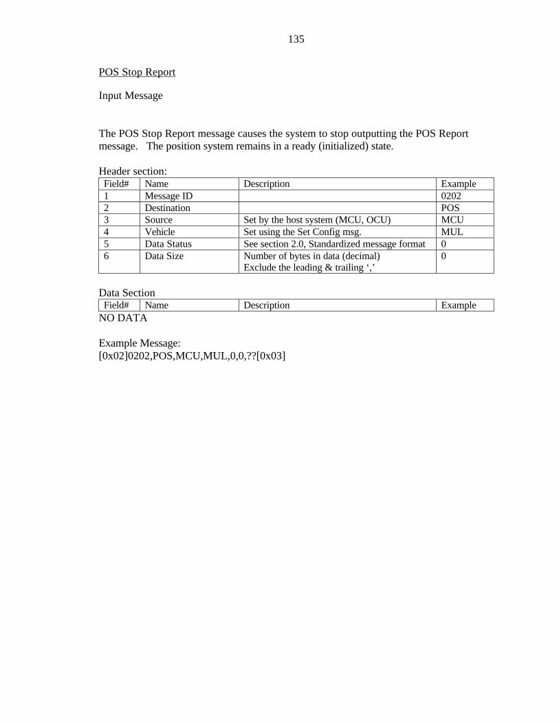
135
POS Stop Report
Input Message The POS Stop Report message causes the system to stop outputting the POS Report message. The position system remains in a ready (initialized) state. Header section: Field# Name Description Example 1 Message ID 0202 2 Destination POS 3 Source Set by the host system (MCU, OCU) MCU 4 Vehicle Set using the Set Config msg. MUL 5 Data Status See section 2.0, Standardized message format 0 6 Data Size Number of bytes in data (decimal)
Exclude the leading & trailing ‘,’ 0
Data Section
Field# Name Description Example NO DATA Example Message: [0x02]0202,POS,MCU,MUL,0,0,??[0x03]
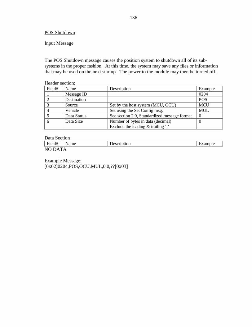
136
POS Shutdown
Input Message The POS Shutdown message causes the position system to shutdown all of its sub-systems in the proper fashion. At this time, the system may save any files or information that may be used on the next startup. The power to the module may then be turned off. Header section: Field# Name Description Example 1 Message ID 0204 2 Destination POS 3 Source Set by the host system (MCU, OCU) MCU 4 Vehicle Set using the Set Config msg. MUL 5 Data Status See section 2.0, Standardized message format 0 6 Data Size Number of bytes in data (decimal)
Exclude the leading & trailing ‘,’ 0
Data Section
Field# Name Description Example NO DATA Example Message: [0x02]0204,POS,OCU,MUL,0,0,??[0x03]
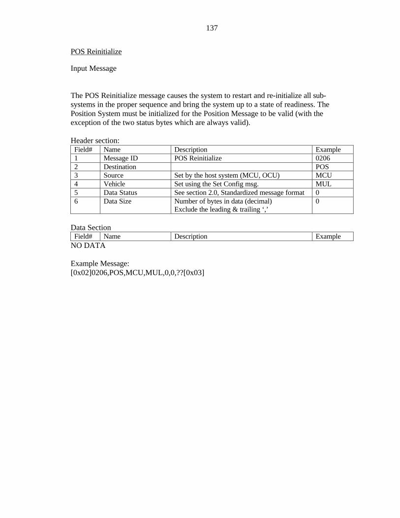
137
POS Reinitialize
Input Message The POS Reinitialize message causes the system to restart and re-initialize all sub-systems in the proper sequence and bring the system up to a state of readiness. The Position System must be initialized for the Position Message to be valid (with the exception of the two status bytes which are always valid). Header section: Field# Name Description Example 1 Message ID POS Reinitialize 0206 2 Destination POS 3 Source Set by the host system (MCU, OCU) MCU 4 Vehicle Set using the Set Config msg. MUL 5 Data Status See section 2.0, Standardized message format 0 6 Data Size Number of bytes in data (decimal)
Exclude the leading & trailing ‘,’ 0
Data Section
Field# Name Description Example NO DATA Example Message: [0x02]0206,POS,MCU,MUL,0,0,??[0x03]

138
POS Standby
Input Message The POS Standby message causes the system to go into a standby mode. In standby mode the system is alive and ready to be re-initialized. Note: A POS Shutdown should be given prior to turning system power off. Header section: Field# Name Description Example 1 Message ID 0208 2 Destination POS 3 Source Set by the host system (MCU, OCU) MCU 4 Vehicle Set using the Set Config msg. MUL 5 Data Status See section 2.0, Standardized message format 0 6 Data Size Number of bytes in data (decimal)
Exclude the leading & trailing ‘,’ 0
Data Section
Field# Name Description Example NO DATA Example Message: [0x02]0208,POS,MCU,MUL,0,0,??[0x03]

139
POS Set Configuration
Input Message The POS Set Configuration message is used to set up the configuration of the system. The following gives an explanation of the parameters: Header section: Field# Name Description Example 1 Message ID 020A 2 Destination POS 3 Source Set by the host system (MCU, OCU) MCU 4 Vehicle Set using the Set Config msg. MUL 5 Data Status See section 2.0, Standardized message format 0 6 Data Size Variable, set prior to shipping (use sizeof()) ??
Data Section
Field# Name Description Example 7 Vehicle The system that the module is physically
contained in. MUL
8 Reference Latitude degrees This may be given to specify the location of a base station (if a DGPS is used) or perhaps the reference offset if a non-absolute position system is used. The definition would be given by the particular position system documentation.
29.123456
9 Reference Longitude degrees -82.123456 10 ReferenceElevation meters 27.123 11 # Sensors # of sensors requiring an offset 1 12 Position Offset X1 meters
The position offsets give the location of a sensor relative to a coordinate system on the vehicle that the user chooses. All of the sensors must be referenced to the same coordinate system. In other words, the user chooses a coordinate system anywhere on the vehicle, then measures the offsets to each of the position system sensors used.
-2.123
13 Position Offset Y1 meters Note: The location of the coordinate system chosen will be the output of the module.
1.123
14 Position Offset Z1 meters Note: A sensor placed at the origin and oriented with the axis, has a zero offsets
0.123
15 Angular OffsetX1-Axis
radians The angular offsets give the rotation of a sensor relative to the same coordinate system
0.0

140
on the vehicle that the user chooses. All of the sensors must be referenced to the same coordinate system.
16 Angular OffsetY1-Axis
radians 0.0
17 Angular OffsetZ1-Axis
radians 0.0
18 Pos. Offset Xn 1.123 19 Pos. Offset Yn -1.123 20 Pos. Offset Zn 0.123 21 Angular OffsetXn-
Axis 0.0
22 Angular OffsetYn-Axis
0.0
23 Angular OffsetZn-Axis
0.0
Example Message: [0x02]020A,POS,MCU,MUL,0,??,,MUL,29.1234567, -82.1234567 27.123,2,-2.123,1.123,0.123,0.0,0.0,0.0,??[0x03]

141
POS Request Configuration
Input Message This message is used to request the current configuration of the position system. See POS Configuration Report for the response definition. Header section: Field# Name Description Example 1 Message ID 020C 2 Destination POS 3 Source Set by the host system (MCU, OCU) MCU 4 Vehicle Set using the Set Config msg. MUL 5 Data Status See section 2.0, Standardized message format 0 6 Data Size Number of bytes in data (decimal)
Exclude the leading & trailing ‘,’ 0
Data Section
Field# Name Description Example NO DATA Example Message: [0x02]020C,POS,MCU,MUL,0,0,??[0x03]

142
POS Request Status
Input Message This message is used to request the current status of the position system. See the POS Status Report for the response definition. Header section: Field# Name Description Example 1 Message ID 020E 2 Destination POS 3 Source Set by the host system (MCU, OCU) MCU 4 Vehicle Set using the Set Config msg. MUL 5 Data Status See section 2.0, Standardized message format 0 6 Data Size Number of bytes in data (decimal)
Exclude the leading & trailing ‘,’ 0
Data Section
Field# Name Description Example NO DATA Example Message: [0x02]020E,POS,MCU,MUL,0,0,??[0x03]

143
POS Report
Output Message This is the main message from the position system. The following is a description of the parameters: Header section:
Field# Name Description Example 1 Message ID 02A0 2 Destination Destination will be set equal to the source of
the start Report message MCU
3 Source POS 4 Vehicle Set using the Set Config msg. MUL 5 Data Status See section 2.0, Standardized message format 0 6 Data Size Variable, set prior to shipping ??
Data Section
Field# Name Description Example 7 Latitude degrees.
The current latitude in WGS-84 geodetic coordinates
29.123456
8 Longitude degrees The current latitude in WGS-84 geodetic coordinates.
-85.123456
9 Elevation meters ellipsoid height
23.12
10 Position RMS meters 0.03 11 theta_x (roll) radians
-π/2 to π/2 Uses the right hand rule, x is forward, z is down (axis attached to vehicle)
1.12
12 theta_y (pitch) radians -π /2 to π/2
1.12
13 theta_z (yaw) radians 0 to 2π 0 = Geodetic North
3.12
14 theta RMS radians 0.01 15 vel_x (meters/sec)
The instantaneous velocity of the vehicle in the direction of the vehicle’s x-axis. The three linear velocity parameters define the first half of the velocity state. The second half is defined by omega_x, omega_y, and omega_z, the rotational rates about the axes.
2.12
16 vel_y meters/sec 2.12 17 vel_z meters/sec 0.12 18 velocity RMS meters/sec 0.02

144
19 omega_x rad/sec The rotational rate about the x-axis of the vehicle.
0.23
20 omega_y rad/sec The rotational rate about the y-axis of the vehicle.
0.5
21 omega_z rad/sec The rotational rate about the z-axis of the vehicle.
0.6
22 Omega RMS radians/sec 23 Time Stamp Julion Time (hhmmssss)
The time when the position data was valid. 12201022
24 Status See Below 01 Example Message: [0x02]02a0,MCU,POS,MUL,0,??,29.1234567,-85.1234567,23.12,0.03 1.12,1.12,3.12,0.01,2.12,2.12,0.12,0.02,0.23,0.5,0.6,12201022,01,??[0x03] 24. Status Byte Description: Status byte 1 is generic and will not change from system to system. Status byte 2 is set aside to be system specific defined by the various POS system modules. Message....[s1][s2] Status Bytes 1 and 2 Status Byte 1 Status Byte 2 Bit Condition when set (1 = set) Bit Condition when set (1=set) 0 Startup 0 Contractor Reserved 1 Busy 1 Contractor Reserved 2 Standby 2 Contractor Reserved 3 Ready 3 Contractor Reserved 4 Problem 4 Contractor Reserved 5 Error 5 Contractor Reserved 6 Failure 6 Contractor Reserved 7 Shutdown 7 Contractor Reserved
Description:
Startup: Indicates the system has just been powered up Busy: Indicates the system is currently processing the last command Standby: Indicates the following statements apply:
- The system is ready to be reinitialized - The Position Report message is not valid (with the exception of the two status bytes that are always valid)
Ready: Indicates that the system is initialized and is operational Problem: Indicates that a self-correcting problem has occurred and the
problem is being corrected internally. This problem requires no input from the host

145
Error: Indicates that a problem has occurred that the system could not resolve. An error requires the intervention of the host to be resolved.
Failure: Indicates that the system has failed and will not recover.
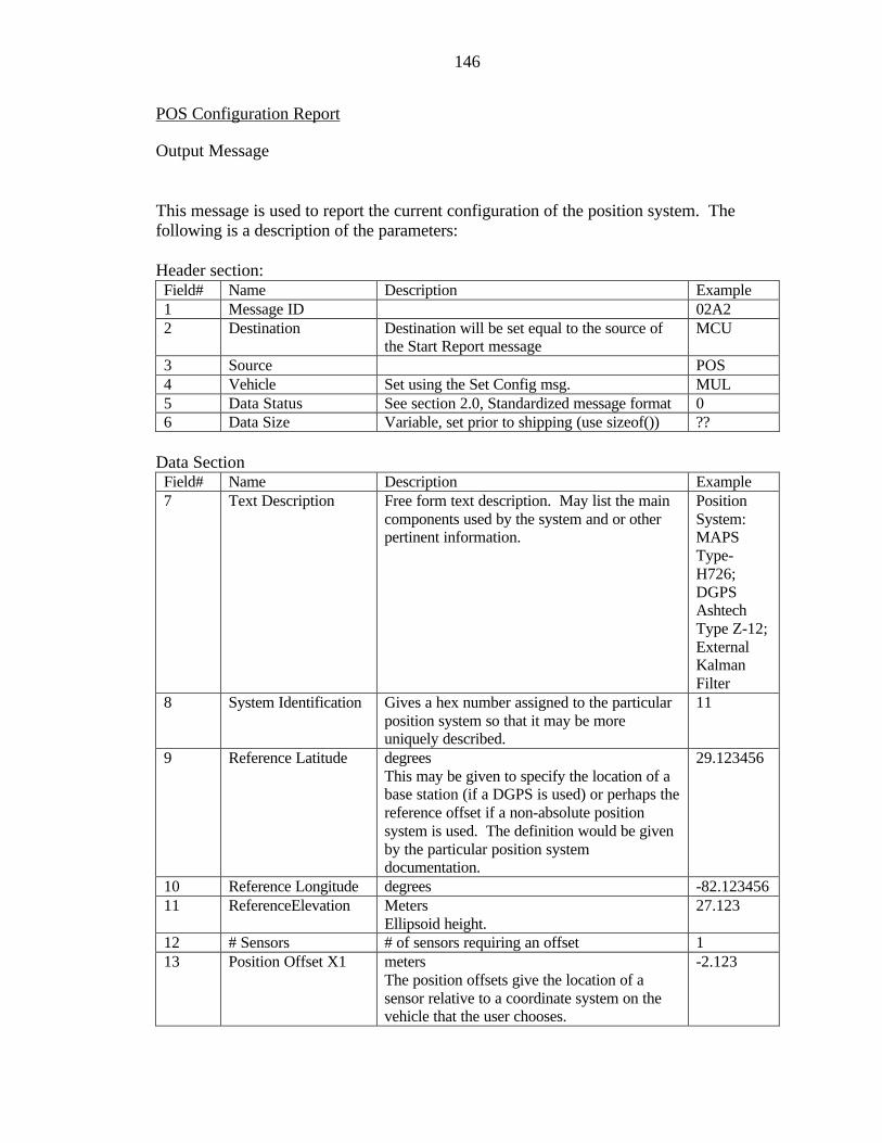
146
POS Configuration Report
Output Message This message is used to report the current configuration of the position system. The following is a description of the parameters: Header section: Field# Name Description Example 1 Message ID 02A2 2 Destination Destination will be set equal to the source of
the Start Report message MCU
3 Source POS 4 Vehicle Set using the Set Config msg. MUL 5 Data Status See section 2.0, Standardized message format 0 6 Data Size Variable, set prior to shipping (use sizeof()) ??
Data Section
Field# Name Description Example 7 Text Description Free form text description. May list the main
components used by the system and or other pertinent information.
Position System: MAPS Type-H726; DGPS Ashtech Type Z-12; External Kalman Filter
8 System Identification Gives a hex number assigned to the particular position system so that it may be more uniquely described.
11
9 Reference Latitude degrees This may be given to specify the location of a base station (if a DGPS is used) or perhaps the reference offset if a non-absolute position system is used. The definition would be given by the particular position system documentation.
29.123456
10 Reference Longitude degrees -82.123456 11 ReferenceElevation Meters
Ellipsoid height. 27.123
12 # Sensors # of sensors requiring an offset 1 13 Position Offset X1 meters
The position offsets give the location of a sensor relative to a coordinate system on the vehicle that the user chooses.
-2.123

147
14 Position Offset Y1 meters Note: The location of the coordinate system chosen will be the output of the module.
1.123
15 Position Offset Z1 meters Note: A sensor placed at the origin and oriented with the axis, requires no offsets.
0.123
16 Angular OffsetX1-Axis
radians The angular offsets give the rotation of a sensor relative to the coordinate system on the vehicle that the user chooses.
0.0
17 Angular OffsetY1-Axis
radians 0.0
18 Angular OffsetZ1-Axis
radians 0.0
19 Pos. Offset Xn 1.123 20 Pos. Offset Yn -1.123 21 Pos. Offset Zn 0.123 22 Angular OffsetXn-
Axis 0.0
23 Angular OffsetYn-Axis
0.0
24 Angular OffsetZn-Axis
0.0
Example Message: [0x02]02A2,MCU,POS,MUL,0,??,Position System: MAPS Type-H726; DGPS Ashtech Type Z-12; External Kalman Filter,11,29.1234567,-85.1234567,27.123,1, -2.123,1.123,0.123,0.0,0.0,0.0,??[0x03]
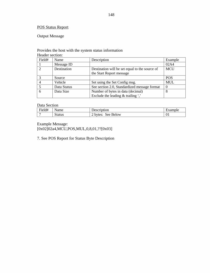
148
POS Status Report
Output Message Provides the host with the system status information Header section: Field# Name Description Example 1 Message ID 02A4 2 Destination Destination will be set equal to the source of
the Start Report message MCU
3 Source POS 4 Vehicle Set using the Set Config msg. MUL 5 Data Status See section 2.0, Standardized message format 0 6 Data Size Number of bytes in data (decimal)
Exclude the leading & trailing ‘,’ 8
Data Section
Field# Name Description Example 7 Status 2 bytes: See Below 01
Example Message: [0x02]02a4,MCU,POS,MUL,0,8,01,??[0x03] 7. See POS Report for Status Byte Description

149
2.3 Mobility Control Unit (MCU) (ASCII)
Version 2.0 The Mobility Control Unit (MCU) is essentially the supervisor for the mobility task. A user may interact with the system by sending messages from the Operator Control Unit (OCU) or other supervisory component. The MCU then issues directives to the other sub-modules of the system. This section of the report serves to document the many messages that can be sent to and from the MCU. The messages that are input to the MCU and that are sent from the MCU are organized below according to the component that the message communicates with. I. Input Messages:
A. Inputs from the OCU component - MCU Start Report - 0x0300 - MCU Stop Report - 0x0302 - MCU Shutdown - 0x0304 - MCU Reinitialize - 0x0306 - MCU Standby - 0x0308 - MCU Set Config. - 0x030a - MCU Request Config. - 0x030c - MCU Request Status - 0x030e - MCU Execute Path - 0x0320 - MCU Pause - 0x0322 - MCU Continue - 0x0324 - MCU Set Mode - 0x0326
- All VCU input messages - See VCU interface document
- All POS input messages - See POS interface document.
- ALL DMS input messages - See DMS interface document.
- All PLN input messages - See PLN interface document
B. Inputs from the VCU component
- All VCU output Messages - See VCU interface document
C. Inputs from the POS component - All POS output messages - See POS interface document
D. Inputs from the DMS component - All DMS output messages - See DMS interface document. - POSStart - See POS interface document.
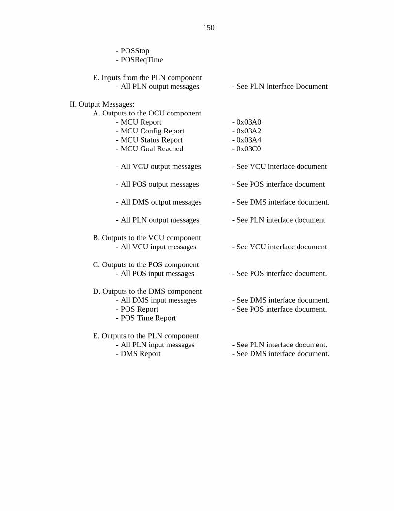
150
- POSStop - POSReqTime
E. Inputs from the PLN component
- All PLN output messages - See PLN Interface Document II. Output Messages:
A. Outputs to the OCU component - MCU Report - 0x03A0 - MCU Config Report - 0x03A2 - MCU Status Report - 0x03A4 - MCU Goal Reached - 0x03C0
- All VCU output messages - See VCU interface document
- All POS output messages - See POS interface document
- All DMS output messages - See DMS interface document.
- All PLN output messages - See PLN interface document
B. Outputs to the VCU component
- All VCU input messages - See VCU interface document
C. Outputs to the POS component - All POS input messages - See POS interface document.
D. Outputs to the DMS component
- All DMS input messages - See DMS interface document. - POS Report - See POS interface document. - POS Time Report
E. Outputs to the PLN component
- All PLN input messages - See PLN interface document. - DMS Report - See DMS interface document.
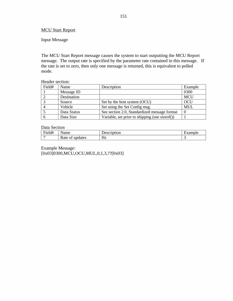
151
MCU Start Report
Input Message The MCU Start Report message causes the system to start outputting the MCU Report message. The output rate is specified by the parameter rate contained in this message. If the rate is set to zero, then only one message is returned, this is equivalent to polled mode. Header section: Field# Name Description Example 1 Message ID 0300 2 Destination MCU 3 Source Set by the host system (OCU) OCU 4 Vehicle Set using the Set Config msg. MUL 5 Data Status See section 2.0, Standardized message format 0 6 Data Size Variable, set prior to shipping (use sizeof()) 1
Data Section
Field# Name Description Example 7 Rate of updates Hz 3
Example Message: [0x03]0300,MCU,OCU,MUL,0,1,3,??[0x03]
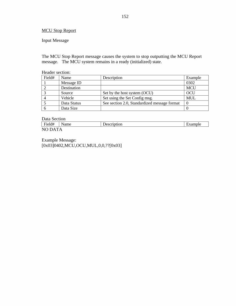
152
MCU Stop Report
Input Message The MCU Stop Report message causes the system to stop outputting the MCU Report message. The MCU system remains in a ready (initialized) state. Header section: Field# Name Description Example 1 Message ID 0302 2 Destination MCU 3 Source Set by the host system (OCU) OCU 4 Vehicle Set using the Set Config msg. MUL 5 Data Status See section 2.0, Standardized message format 0 6 Data Size 0
Data Section
Field# Name Description Example NO DATA Example Message: [0x03]0402,MCU,OCU,MUL,0,0,??[0x03]

153
MCU Shutdown
Input Message The MCU Shutdown message causes the MCU system to shutdown all of its sub-systems in the proper fashion. At this time, the system may save any files or information that may be used on the next startup. The power to the module may then be turned off. Header section:
Field# Name Description Example 1 Message ID 0304 2 Destination MCU 3 Source Set by the host system (OCU) OCU 4 Vehicle Set using the Set Config msg. MUL 5 Data Status See section 2.0, Standardized message format 0 6 Data Size 0
Data Section
Field# Name Description Example NO DATA Example Message: [0x03]0304,MCU,OCU,MUL,0,0,??[0x03]

154
MCU Reinitialize
Input Message The MCU Reinitialize message causes the system to restart and re-initialize all sub-systems in the proper sequence and bring the system up to a state of readiness. Note: The MCU may elect to check sub-system status and decide weather or not a re-initialize is necessary for each sub-system. Header section: Field# Name Description Example 1 Message ID 0306 2 Destination MCU 3 Source Set by the host system (OCU) OCU 4 Vehicle Set using the Set Config msg. MUL 5 Data Status See section 2.0, Standardized message format 0 6 Data Size 0
Data Section
Field# Name Description Example NO DATA Example Message: [0x03]0306,MCU,OCU,MUL,0,0,??[0x03]
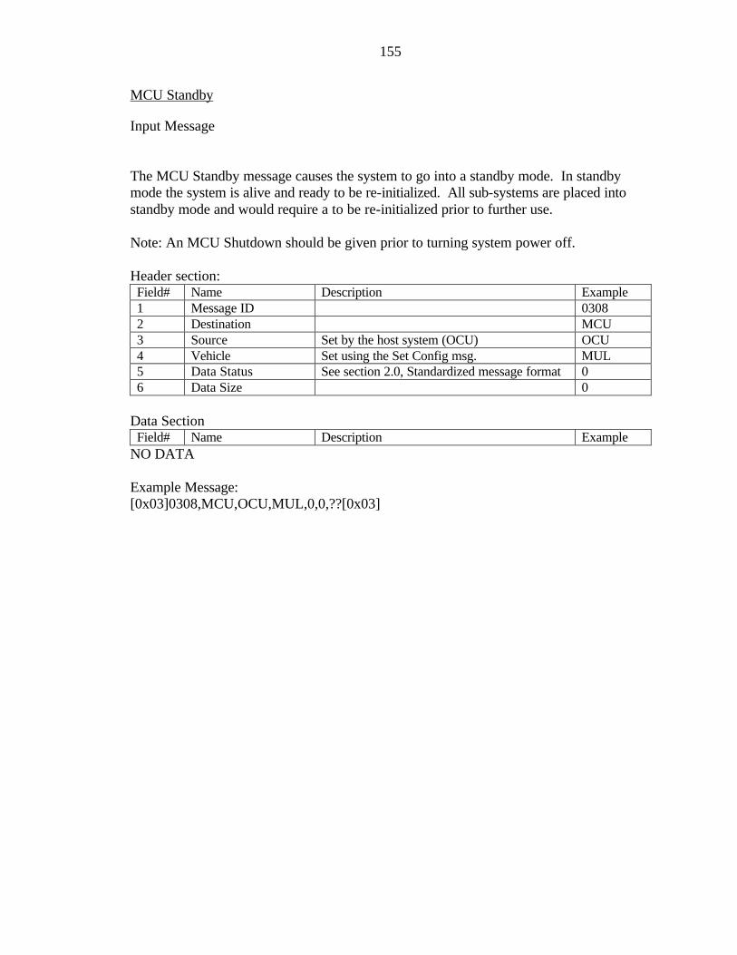
155
MCU Standby
Input Message The MCU Standby message causes the system to go into a standby mode. In standby mode the system is alive and ready to be re-initialized. All sub-systems are placed into standby mode and would require a to be re-initialized prior to further use. Note: An MCU Shutdown should be given prior to turning system power off. Header section: Field# Name Description Example 1 Message ID 0308 2 Destination MCU 3 Source Set by the host system (OCU) OCU 4 Vehicle Set using the Set Config msg. MUL 5 Data Status See section 2.0, Standardized message format 0 6 Data Size 0
Data Section
Field# Name Description Example NO DATA Example Message: [0x03]0308,MCU,OCU,MUL,0,0,??[0x03]

156
MCU Set Configuration
Input Message The MCU Set Configuration message is used to set up the configuration of the system. The following gives an explanation of the parameters: Header section: Field# Name Description Example 1 Message ID 030A 2 Destination MCU 3 Source Set by the host system (OCU) OCU 4 Vehicle Set using the Set Config msg. MUL 5 Data Status See section 2.0, Standardized message format 0 6 Data Size Variable, set prior to shipping (use sizeof()) 3
Data Section
Field# Name Description Example 7 Vehicle The system that the module is physically
contained in. MUL
Example Message: [0x03]030A,MCU,OCU,MUL,0,3,MUL,??[0x03]

157
MCU Request Configuration
Input Message This message is used to request the current configuration of the MCU system. See MCU Configuration Report for the response definition. Header section: Field# Name Description Example 1 Message ID 030C 2 Destination MCU 3 Source Set by the host system (MCU, OCU) OCU 4 Vehicle Set using the Set Config msg. MUL 5 Data Status See section 2.0, Standardized message format 0 6 Data Size 0
Data Section
Field# Name Description Example NO DATA Example Message: [0x03]030C,MCU,OCU,MUL,0,0,?? [0x03]

158
MCU Request Status
Input Message This message is used to request the current status of the MCU system. See MCU Status Report for the response definition. Header section: Field# Name Description Example 1 Message ID 030E 2 Destination MCU 3 Source Set by the host system (MCU, OCU) OCU 4 Vehicle Set using the Set Config msg. MUL 5 Data Status See section 2.0, Standardized message format 0 6 Data Size 0
Data Section
Field# Name Description Example NO DATA Example Message: [0x03]030E,MCU,OCU,MUL,0,0,??[0x03]

159
MCU Execute Path
Input Message MCU Execute Path causes the vehicle to begin execution of the path. The path executed is the one currently loaded on the MCU unless a path is given in this message. Header section: Field# Name Description Example 1 Message ID 0320 2 Destination MCU 3 Source Set by the host system (MCU, OCU) OCU 4 Vehicle Set using the Set Config msg. MUL 5 Data Status See section 2.0, Standardized message format 0 6 Data Size Variable ??
Data Section
Field# Name Description Example 7 Desired Vehicle Sped meters/sec 3.0 8 # sub-goals The number of points that make up the path
Note: If zero, then execute existing path on Destination is used.
250
9 Latitude #1 degrees Latitude of the first sub-goal. (WGS-84)
29.123456
10 Longitude #1 degrees Longitude of the first sub-goal. (WGS-84)
-85.123456
11 Altitude #1 meters Altitude of the first sub-goal.
23.12
12 theta_x (roll) radians Orientation about the x-axis, -π/2 to π/2. Use the right hand rule, x is forward, z is down (axis attached to vehicle)
1.12
13 theta_y (pitch) radians Orientation about the y-axis, -π/2 to π/2.
1.12
14 theta_z (yaw) radians Orientation about the z-axis, 0 to 2.0π. 0 = Geodetic North
3.12
?? Latitude #n 29.123456 ?? Longitude #n -85.123456 ?? Altitude #n 23.12 ?? theta_x (roll) 1.12 ?? theta_y (pitch) 1.12 ?? theta_z (yaw) 3.12
Example Message: [0x03]0320,MCU,OCU,MUL,0,??,3.0,250,29.1234567,85.1234567,23.12,1.12,1.12,3.12..??[0x03]

160
MCU Pause
Input Message This message causes the vehicle to stop path execution. It is meant to be used as a temporary stop (pause). The MCU’s sub-systems will remain in the active (ready) state so that path execution can continue immediately upon receipt of the MCU Continue message. If a more secure state is desired than a MCU Standby message should be used as this will place all of the MCU’s sub-systems in a safe (Standby) mode. Header section: Field# Name Description Example 1 Message ID 0322 2 Destination MCU 3 Source Set by the host system (MCU, OCU) OCU 4 Vehicle Set using the Set Config msg. MUL 5 Data Status See section 2.0, Standardized message format 0 6 Data Size 0
Data Section
Field# Name Description Example NO DATA Example Message: [0x03]0322,MCU,OCU,MUL,0,0,??[0x03]

161
MCU Continue
Input Message This message is used to resume vehicle motion after receipt of a MCU Pause. Header section: Field# Name Description Example 1 Message ID 0324 2 Destination MCU 3 Source Set by the host system (MCU, OCU) OCU 4 Vehicle Set using the Set Config msg. MUL 5 Data Status See section 2.0, Standardized message format 0 6 Data Size variable ??
Data Section
Field# Name Description Example 7 Vehicle Speed The desired vehicle speed 3.0
Example Message: [0x03]0324,MCU,OCU,MUL,0,??,3.0,??[0x03]
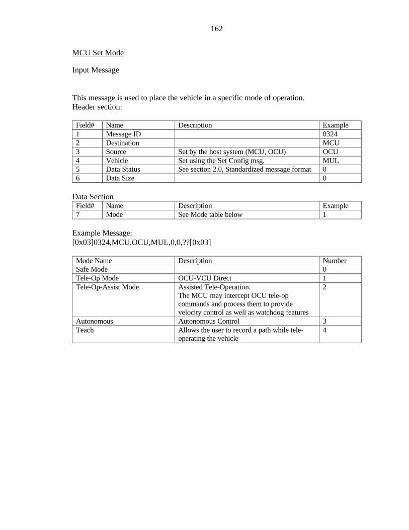
162
MCU Set Mode
Input Message This message is used to place the vehicle in a specific mode of operation. Header section: Field# Name Description Example 1 Message ID 0324 2 Destination MCU 3 Source Set by the host system (MCU, OCU) OCU 4 Vehicle Set using the Set Config msg. MUL 5 Data Status See section 2.0, Standardized message format 0 6 Data Size 0
Data Section
Field# Name Description Example 7 Mode See Mode table below 1
Example Message: [0x03]0324,MCU,OCU,MUL,0,0,??[0x03] Mode Name Description Number Safe Mode 0 Tele-Op Mode OCU-VCU Direct 1 Tele-Op-Assist Mode Assisted Tele-Operation.
The MCU may intercept OCU tele-op commands and process them to provide velocity control as well as watchdog features
2
Autonomous Autonomous Control 3 Teach Allows the user to record a path while tele-
operating the vehicle 4

163
MCU Report
Output Message This message is the MCU report. The following is a description of the parameters: Header section: Field# Name Description Example 1 Message ID 03A0 2 Destination Destination will be set equal to the source of
the Start Report message MCU
3 Source OCU 4 Vehicle Set using the Set Config msg. MUL 5 Data Status See section 2.0, Standardized message format 0 6 Data Size Variable, set prior to shipping (use sizeof()) 11
Data Section
Field# Name Description Example 7 Mode Mode of operation: See table from MCU Set
Mode 1
8 VCU Status See VCU interface Document 10 9 POS Status See POS interface Document 10 10 DMS Status See DMS interface Document 10 11 PLN Status See PLN interface Document 10 12 MCU Status See Below 10
Example Message: [0x03]03a0,MCU,OCU,MUL,0,11,1,10,10,10,10,10,??[0x03] 12. Status Byte Description: Status byte 1 is generic and will not change from system to system. Status byte 2 is set aside to be system specific defined by the various MCU system modules. Message....[s1][s2] Status Bytes 1 and 2 Status Byte 1 Status Byte 2 Bit Condition when set (1 = set) Bit Condition when set (1=set) 0 Startup 0 Contractor Reserved 1 Busy 1 Contractor Reserved 2 Standby 2 Contractor Reserved 3 Ready 3 Contractor Reserved 4 Problem 4 Contractor Reserved 5 Error 5 Contractor Reserved 6 Failure 6 Contractor Reserved 7 Shutdown 7 Contractor Reserved

164
Description:
Startup: Indicates the system has just been powered up Busy: Indicates the system is currently processing the last command Standby: Indicates the following statements apply:
- The system is ready to be reinitialize - The system will not respond to commands that cause or resist motion
- The vehicle should remain stationary - The vehicle actuators should not move - From a mobility standpoint, the vehicle should be considered safe
Ready: Indicates that the system is initialized and is operational Problem: Indicates that a self-correcting problem has occurred and the
problem is being corrected internally. This problem requires no input from the host
Error: Indicates that a problem has occurred that the system could not resolve. An error requires the intervention of the host to be resolved.
Failure: Indicates that the system has failed and will not recover.

165
MCU Configuration Report
Output Message This message is used to report the current configuration of the MCU system. The following is a description of the parameters: Header section: Field# Name Description Example 1 Message ID 03A2 2 Destination Destination will be set equal to the source of
the Start Report message MCU
3 Source OCU 4 Vehicle Set using the Set Config msg. MUL 5 Data Status See section 2.0, Standardized message format 0 6 Data Size Variable, set prior to shipping (use sizeof()) ??
Data Section Field# Name Description Example 7 Text Description Free form text description. May list the main
components used by the system and or other pertinent information.
MCU: requires PLN, POS, and VCU modules.
8 System Identification Gives a hex number assigned to the particular MCU system so that it may be more uniquely described.
11
Example Message: [0x03]03A2,MCU,OCU,MUL,0,??,MCU: requires PLN, POS, and VCU modules,11,??[0x03]

166
MCU Status Report
Output Message Provides the host with the system status information Header section: Field# Name Description Example 1 Message ID 03A4 2 Destination Destination will be set equal to the source of
the Start Report message MCU
3 Source OCU 4 Vehicle Set using the Set Config msg. MUL 5 Data Status See section 2.0, Standardized message format 0 6 Data Size 8
Data Section
Field# Name Description Example 7 MCU Status See Below 01
Example Message: [0x03]03a4,MCU,OCU,MUL,0,20,,01,??[0x03] 7. See MCU Report for Status Byte Description

167
2.4 Detection Mapping Systems (DMS) (ASCII)
Version 2.0 This section presents the messages that may be sent to the DMS and the messages that will be returned. Every message will be composed of a header section, a data section, and an end of message section. The data section of the messages are defined here. See the standardized message format documentation (section 2.0) for the header and end of message formats. Note: See specific module documentation for additional (system specific, non required) messages. I. Input Messages:
- DMS Start Report - 0x0400 - DMS Stop Report - 0x0402 - DMS Shutdown - 0x0404 - DMS Reinitialize - 0x0406 - DMS Standby - 0x0408 - DMS Set Config - 0x040A - DMS Request Config - 0x040C - DMS Request Status - 0x040E
- POS Report - See POS interface document
II. Output Messages:
- DMS Report - 0x04A0 - DMS Config Report - 0x04A2 - DMS Status Report - 0x04A4
- POS Start Report - See POS interface document - POS Stop Report

168
DMS Start Report
Input Message The DMS Start Report message causes the system to start outputting the DMS Report message. The output rate is specified by the parameter rate contained in this message. If the rate is set to zero, then only one message is returned, this is equivalent to polled mode. Header section: Field# Name Description Example 1 Message ID 0400 2 Destination DMS 3 Source Set by the host system (MCU, OCU) MCU 4 Vehicle Set using the Set Config msg. MUL 5 Data Status See section 2.0, Standardized message format 0 6 Data Size Number of bytes in data (decimal)
Exclude the leading & trailing ‘,’ ??
Data Section
Field# Name Description Example 7 Rate of updates Hz
The first report will include all of the changes to the Map since the given time and then each report that follows will include only new information.
0.5
8 Time Julion time, hhmmssss Request all changes to the Global Map since this time.
12012019
9 Classifications The DMS will report only changes to the Global Map with this classification. Used to narrow the Global Map report. For example: Request a Global Map report of just the obstacles that classified as a tree. Note: 0=all classifications See Classification table.
0
Example Message: [0x02]0400,DMS,MCU,MUL,0,10,5,12012019,0,??[0x03]

169
DMS Stop Report
Input Message The DMS Stop Report message causes the system to stop outputting the DMS Report message. The DMS remains in a ready (initialized) state. Header section: Field# Name Description Example 1 Message ID 0402 2 Destination DMS 3 Source Set by the host system (MCU, OCU) MCU 4 Vehicle Set using the Set Config msg. MUL 5 Data Status See section 2.0, Standardized message format 0 6 Data Size Number of bytes in data (decimal)
Exclude the leading & trailing ‘,’ 0
Data Section
Field# Name Description Example NO DATA Example Message: [0x02]0402,DMS,MCU,MUL,0,0,??[0x03]

170
DMS Shutdown
Input Message The DMS Shutdown message causes the DMS to shutdown all of its sub-systems in the proper fashion. At this time, the system may save any files or information that may be used on the next startup. The power to the module may then be turned off. Header section: Field# Name Description Example 1 Message ID 0404 2 Destination DMS 3 Source Set by the host system (MCU, OCU) MCU 4 Vehicle Set using the Set Config msg. MUL 5 Data Status See section 2.0, Standardized message format 0 6 Data Size Number of bytes in data (decimal)
Exclude the leading & trailing ‘,’ 0
Data Section
Field# Name Description Example NO DATA Example Message: [0x02]0404,DMS,OCU,MUL,0,0,??[0x03]

171
DMS Reinitialize
Input Message The DMS Reinitialize message causes the system to restart and re-initialize all sub-systems in the proper sequence and bring the system up to a state of readiness. Header section: Field# Name Description Example 1 Message ID 0406 2 Destination DMS 3 Source Set by the host system (MCU, OCU) MCU 4 Vehicle Set using the Set Config msg. MUL 5 Data Status See section 2.0, Standardized message format 0 6 Data Size Number of bytes in data (decimal)
Exclude the leading & trailing ‘,’ 0
Data Section
Field# Name Description Example NO DATA Example Message: [0x02]0406,DMS,MCU,MUL,0,0,??[0x03]

172
DMS Standby
Input Message The DMS Standby message causes the system to go into a standby mode. In standby mode the system is alive and ready to be re-initialized. Note: A DMS Shutdown should be given prior to turning system power off. Header section: Field# Name Description Example 1 Message ID 0408 2 Destination DMS 3 Source Set by the host system (MCU, OCU) MCU 4 Vehicle Set using the Set Config msg. MUL 5 Data Status See section 2.0, Standardized message format 0 6 Data Size Number of bytes in data (decimal)
Exclude the leading & trailing ‘,’ 0
Data Section
Field# Name Description Example NO DATA Example Message: [0x02]0408,DMS,MCU,MUL,0,0,??[0x03]
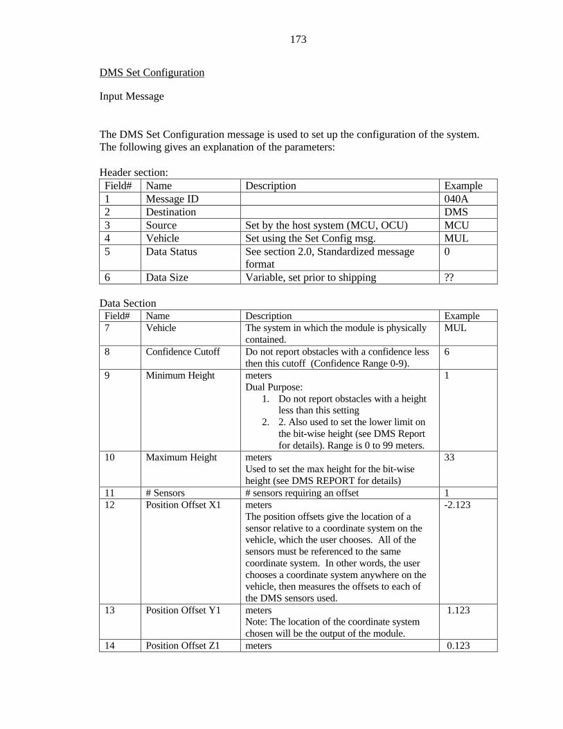
173
DMS Set Configuration
Input Message The DMS Set Configuration message is used to set up the configuration of the system. The following gives an explanation of the parameters: Header section: Field# Name Description Example 1 Message ID 040A 2 Destination DMS 3 Source Set by the host system (MCU, OCU) MCU 4 Vehicle Set using the Set Config msg. MUL 5 Data Status See section 2.0, Standardized message
format 0
6 Data Size Variable, set prior to shipping ?? Data Section
Field# Name Description Example 7 Vehicle The system in which the module is physically
contained. MUL
8 Confidence Cutoff Do not report obstacles with a confidence less then this cutoff (Confidence Range 0-9).
6
9 Minimum Height meters Dual Purpose:
1. Do not report obstacles with a height less than this setting
2. 2. Also used to set the lower limit on the bit-wise height (see DMS Report for details). Range is 0 to 99 meters.
1
10 Maximum Height meters Used to set the max height for the bit-wise height (see DMS REPORT for details)
33
11 # Sensors # sensors requiring an offset 1 12 Position Offset X1 meters
The position offsets give the location of a sensor relative to a coordinate system on the vehicle, which the user chooses. All of the sensors must be referenced to the same coordinate system. In other words, the user chooses a coordinate system anywhere on the vehicle, then measures the offsets to each of the DMS sensors used.
-2.123
13 Position Offset Y1 meters Note: The location of the coordinate system chosen will be the output of the module.
1.123
14 Position Offset Z1 meters 0.123

174
Note: A sensor placed at the origin and oriented with the axis, has all zero offsets
15 Angular OffsetX1-Axis
radians The angular offsets give the rotation of a sensor relative to the same coordinate system on the vehicle, which the user chooses. All of the sensors must be referenced to the same coordinate system.
0.0
16 Angular OffsetY1-Axis
radians 0.0
17 Angular OffsetZ1-Axis
radians 0.0
18 Position Offset Xn 1.123 19 Position Offset Yn -1.123 20 Position Offset Zn 0.123 21 Angular OffsetXn-
Axis 0.0
22 Angular OffsetYn-Axis
0.0
23 Angular OffsetZn-Axis
0.0
Example Message: [0x02]040A,DMS,MCU,MUL,0,??,MUL,6,1,33,1,-2.123,1.123,0.123,0.0,0.0,0.0,.. ...1.123,-1.123,0.123,0.0,0.0,0.0,??[0x03]

175
DMS Request Configuration
Input Message This message is used to request the current configuration of the DMS. See DMS Configuration Report for the response definition. Header section: Field# Name Description Example 1 Message ID 040C 2 Destination DMS 3 Source Set by the host system (MCU, OCU) MCU 4 Vehicle Set using the Set Config msg. MUL 5 Data Status See section 2.0, Standardized message format 0 6 Data Size Number of bytes in data (decimal)
Exclude the leading & trailing ‘,’ 0
Data Section
Field# Name Description Example NO DATA Example Message: [0x02]040C,DMS,MCU,MUL,0,0,?? [0x03]

176
DMS Request Status
Input Message This message is used to request the current status of the DMS. See DMS Status Report for the response definition. Header section: Field# Name Description Example 1 Message ID 040E 2 Destination DMS 3 Source Set by the host system (MCU, OCU) MCU 4 Vehicle Set using the Set Config msg. MUL 5 Data Status See section 2.0, Standardized message format 0 6 Data Size Number of bytes in data (decimal)
Exclude the leading & trailing ‘,’ 0
Data Section Field# Name Description Example NO DATA Example Message: [0x02]040E,DMS,MCU,MUL,0,0,??[0x03]
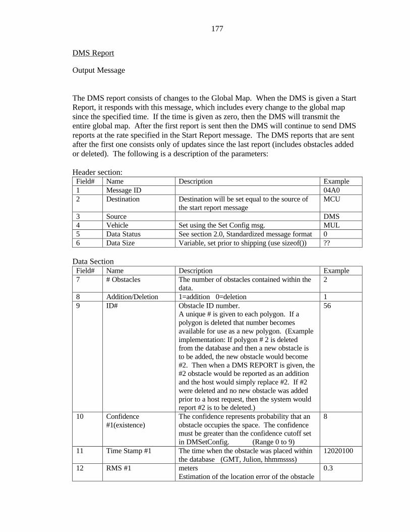
177
DMS Report
Output Message The DMS report consists of changes to the Global Map. When the DMS is given a Start Report, it responds with this message, which includes every change to the global map since the specified time. If the time is given as zero, then the DMS will transmit the entire global map. After the first report is sent then the DMS will continue to send DMS reports at the rate specified in the Start Report message. The DMS reports that are sent after the first one consists only of updates since the last report (includes obstacles added or deleted). The following is a description of the parameters: Header section: Field# Name Description Example 1 Message ID 04A0 2 Destination Destination will be set equal to the source of
the start report message MCU
3 Source DMS 4 Vehicle Set using the Set Config msg. MUL 5 Data Status See section 2.0, Standardized message format 0 6 Data Size Variable, set prior to shipping (use sizeof()) ??
Data Section
Field# Name Description Example 7 # Obstacles The number of obstacles contained within the
data. 2
8 Addition/Deletion 1=addition 0=deletion 1 9 ID# Obstacle ID number.
A unique # is given to each polygon. If a polygon is deleted that number becomes available for use as a new polygon. (Example implementation: If polygon # 2 is deleted from the database and then a new obstacle is to be added, the new obstacle would become #2. Then when a DMS REPORT is given, the #2 obstacle would be reported as an addition and the host would simply replace #2. If #2 were deleted and no new obstacle was added prior to a host request, then the system would report #2 is to be deleted.)
56
10 Confidence #1(existence)
The confidence represents probability that an obstacle occupies the space. The confidence must be greater than the confidence cutoff set in DMSetConfig. (Range 0 to 9)
8
11 Time Stamp #1 The time when the obstacle was placed within the database (GMT, Julion, hhmmssss)
12020100
12 RMS #1 meters Estimation of the location error of the obstacle
0.3
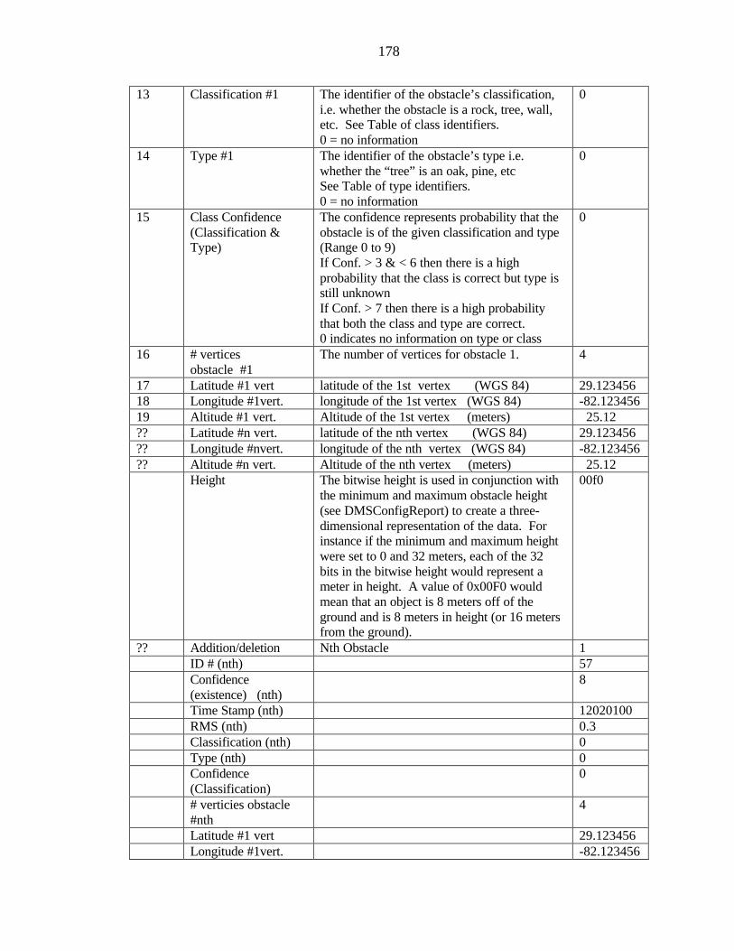
178
13 Classification #1 The identifier of the obstacle’s classification, i.e. whether the obstacle is a rock, tree, wall, etc. See Table of class identifiers. 0 = no information
0
14 Type #1 The identifier of the obstacle’s type i.e. whether the “tree” is an oak, pine, etc See Table of type identifiers. 0 = no information
0
15 Class Confidence (Classification & Type)
The confidence represents probability that the obstacle is of the given classification and type (Range 0 to 9) If Conf. > 3 & < 6 then there is a high probability that the class is correct but type is still unknown If Conf. > 7 then there is a high probability that both the class and type are correct. 0 indicates no information on type or class
0
16 # vertices obstacle #1
The number of vertices for obstacle 1. 4
17 Latitude #1 vert latitude of the 1st vertex (WGS 84) 29.123456 18 Longitude #1vert. longitude of the 1st vertex (WGS 84) -82.123456 19 Altitude #1 vert. Altitude of the 1st vertex (meters) 25.12 ?? Latitude #n vert. latitude of the nth vertex (WGS 84) 29.123456 ?? Longitude #nvert. longitude of the nth vertex (WGS 84) -82.123456 ?? Altitude #n vert. Altitude of the nth vertex (meters) 25.12 Height The bitwise height is used in conjunction with
the minimum and maximum obstacle height (see DMSConfigReport) to create a three-dimensional representation of the data. For instance if the minimum and maximum height were set to 0 and 32 meters, each of the 32 bits in the bitwise height would represent a meter in height. A value of 0x00F0 would mean that an object is 8 meters off of the ground and is 8 meters in height (or 16 meters from the ground).
00f0
?? Addition/deletion Nth Obstacle 1 ID # (nth) 57 Confidence
(existence) (nth) 8
Time Stamp (nth) 12020100 RMS (nth) 0.3 Classification (nth) 0 Type (nth) 0 Confidence
(Classification) 0
# verticies obstacle #nth
4
Latitude #1 vert 29.123456 Longitude #1vert. -82.123456
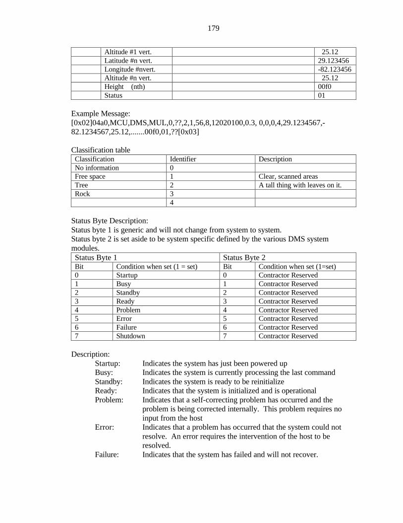
179
Altitude #1 vert. 25.12 Latitude #n vert. 29.123456 Longitude #nvert. -82.123456 Altitude #n vert. 25.12 Height (nth) 00f0 Status 01
Example Message: [0x02]04a0,MCU,DMS,MUL,0,??,2,1,56,8,12020100,0.3, 0,0,0,4,29.1234567,-82.1234567,25.12,.......00f0,01,??[0x03] Classification table Classification Identifier Description No information 0 Free space 1 Clear, scanned areas Tree 2 A tall thing with leaves on it. Rock 3 4
Status Byte Description: Status byte 1 is generic and will not change from system to system. Status byte 2 is set aside to be system specific defined by the various DMS system modules. Status Byte 1 Status Byte 2 Bit Condition when set (1 = set) Bit Condition when set (1=set) 0 Startup 0 Contractor Reserved 1 Busy 1 Contractor Reserved 2 Standby 2 Contractor Reserved 3 Ready 3 Contractor Reserved 4 Problem 4 Contractor Reserved 5 Error 5 Contractor Reserved 6 Failure 6 Contractor Reserved 7 Shutdown 7 Contractor Reserved
Description:
Startup: Indicates the system has just been powered up Busy: Indicates the system is currently processing the last command Standby: Indicates the system is ready to be reinitialize Ready: Indicates that the system is initialized and is operational Problem: Indicates that a self-correcting problem has occurred and the
problem is being corrected internally. This problem requires no input from the host
Error: Indicates that a problem has occurred that the system could not resolve. An error requires the intervention of the host to be resolved.
Failure: Indicates that the system has failed and will not recover.

180
DMS Configuration Report
Output Message This message is used to report the current configuration of the DMS. The following is a description of the parameters: Header section: Field# Name Description Example 1 Message ID 04A2 2 Destination Destination will be set equal to the source of
the start report message MCU
3 Source DMS 4 Vehicle Set using the Set Config msg. MUL 5 Data Status See section 2.0, Standardized message format 0 6 Data Size Variable, set prior to shipping (use sizeof()) ??
Data Section
Field# Name Description Example 7 Text Description Free form text description. May list the main
components used by the system and or other pertinent information.
DMS: JPL Vision, TRC Sonar SICK Laser Takao Fused
8 System Identification Gives a hex number assigned to the particular DMS so that it may be more uniquely described.
2
9 Vehicle See DMSSetConfig MUL 10 Confidence Cutoff See DMSSetConfig 6 11 Minimum Height See DMSSetConfig 1 12 Maximum Height See DMSSetConfig 33 13 # Sensors See DMSSetConfig 3 14 Position Offset X1 See DMSSetConfig -2.123 15 Position Offset Y1 See DMSSetConfig 1.123 16 Position Offset Z1 See DMSSetConfig 0.123 17 Angular OffsetX1-
Axis See DMSSetConfig 0.0
18 Angular OffsetY1-Axis
See DMSSetConfig 0.0
19 Angular OffsetZ1-Axis
See DMSSetConfig 0.0
20 Position Offset Xn See DMSSetConfig 1.123 21 Position Offset Yn See DMSSetConfig -1.123 22 Position Offset Zn See DMSSetConfig 0.123 23 Angular OffsetXn-
Axis See DMSSetConfig 0.0

181
24 Angular OffsetYn-Axis
See DMSSetConfig 0.0
25 Angular OffsetZn-Axis
See DMSSetConfig 0.0
Example Message: [0x02]04A2,MCU,DMS,MUL,0,??,DMS JPL vision TRC sonar SICK laser Takao fused,2,MUL,6,1,33,3,-1.123,1.123,0.123,0.0,0.0,0.0,,..... ......-.123,1.123,0.123,0.0,0.0,0.0,??[0x03]

182
DMS Status Report
Output Message Provides the host with the system status information Header section: Field# Name Description Example 1 Message ID 04A4 2 Destination Destination will be set equal to the source of
the start report message MCU
3 Source DMS 4 Vehicle Set using the Set Config msg. MUL 5 Data Status See section 2.0, Standardized message format 0 6 Data Size Number of bytes in data (decimal)
Exclude the leading & trailing ‘,’ 8
Data Section
Field# Name Description Example 7 Status 2 bytes: See Below 01
Example Message: [0x02]04a4,MCU,DMS,MUL,0,8,01,??[0x03] 7. See DMS Report for Status Byte Description

183
2.5 Path Planner (PLN) (ASCII)
Version 2.0 This section presents the messages that may be sent to the planner system and the messages that will be returned. Every message will be composed of a header section, a data section, and an end of message section. The data section of the messages are defined here. See the standardized message format documentation (section 2.0) for the header and end of message formats. Note: See specific module documentation for additional (system specific, non required) messages. I. Input Messages:
- PLN Shutdown - 0x0504 - PLN Reinitialize - 0x0506 - PLN Set Config. - 0x050A - PLN Request Config. - 0x050C - PLN Request Status - 0x050E
- PLN Request Path - 0x0520
- DMS Report - See Detection Mapping System ID
II. Output Messages:
- PLN Config. Report - 0x05A2 - PLN Status Report - 0x05A4
- PLN Path Report - 0x05C0
- DMS Start Report - See Detection Mapping System ID - DMS Stop Report

184
PLN Shutdown
Input Message The PLN Shutdown message causes the planner system to shutdown all of its sub-systems in the proper fashion. At this time, the system may save any files or information that may be used on the next startup. The power to the module may then be turned off. Header section: Field# Name Description Example 1 Message ID 0504 2 Destination PLN 3 Source Set by the host system (MCU, OCU) MCU 4 Vehicle Set using the Set Config msg. MUL 5 Data Status See section 2.0, Standardized message format 0 6 Data Size Number of bytes in data (decimal)
Exclude the leading & trailing ‘,’ 0
Data Section
Field# Name Description Example NO DATA Example Message: [0x05]0504,PLN,OCU,MUL,0,0,??[0x03]

185
PLN Reinitialize
Input Message The PLN Reinitialize message causes the system to restart and re-initialize all sub-systems in the proper sequence and bring the system up to a state of readiness. Header section: Field# Name Description Example 1 Message ID 0506 2 Destination PLN 3 Source Set by the host system (MCU, OCU) MCU 4 Vehicle Set using the Set Config msg. MUL 5 Data Status See section 2.0, Standardized message format 0 6 Data Size Number of bytes in data (decimal)
Exclude the leading & trailing ‘,’ 0
Data Section
Field# Name Description Example Example Message: [0x05]0506,PLN,MCU,MUL,0,0,??[0x03]
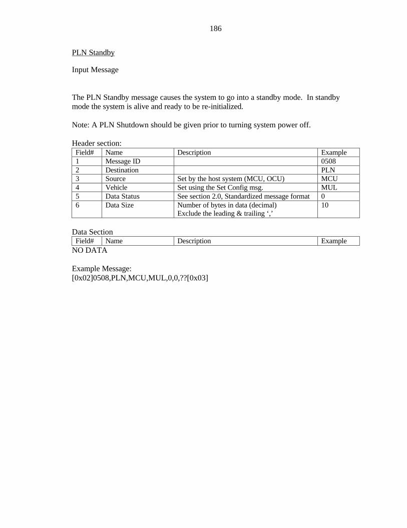
186
PLN Standby
Input Message The PLN Standby message causes the system to go into a standby mode. In standby mode the system is alive and ready to be re-initialized. Note: A PLN Shutdown should be given prior to turning system power off. Header section: Field# Name Description Example 1 Message ID 0508 2 Destination PLN 3 Source Set by the host system (MCU, OCU) MCU 4 Vehicle Set using the Set Config msg. MUL 5 Data Status See section 2.0, Standardized message format 0 6 Data Size Number of bytes in data (decimal)
Exclude the leading & trailing ‘,’ 10
Data Section
Field# Name Description Example NO DATA Example Message: [0x02]0508,PLN,MCU,MUL,0,0,??[0x03]
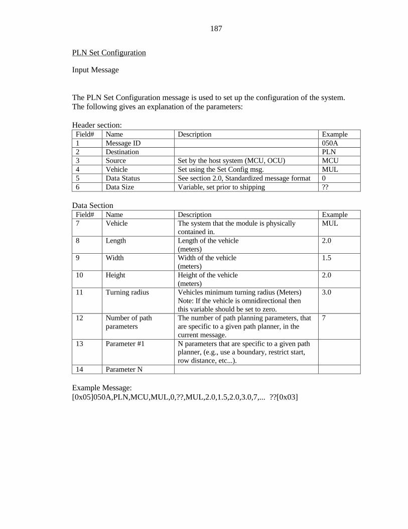
187
PLN Set Configuration
Input Message The PLN Set Configuration message is used to set up the configuration of the system. The following gives an explanation of the parameters: Header section: Field# Name Description Example 1 Message ID 050A 2 Destination PLN 3 Source Set by the host system (MCU, OCU) MCU 4 Vehicle Set using the Set Config msg. MUL 5 Data Status See section 2.0, Standardized message format 0 6 Data Size Variable, set prior to shipping ??
Data Section
Field# Name Description Example 7 Vehicle The system that the module is physically
contained in. MUL
8 Length Length of the vehicle (meters)
2.0
9 Width Width of the vehicle (meters)
1.5
10 Height Height of the vehicle (meters)
2.0
11 Turning radius Vehicles minimum turning radius (Meters) Note: If the vehicle is omnidirectional then this variable should be set to zero.
3.0
12 Number of path parameters
The number of path planning parameters, that are specific to a given path planner, in the current message.
7
13 Parameter #1 N parameters that are specific to a given path planner, (e.g., use a boundary, restrict start, row distance, etc...).
14 Parameter N Example Message: [0x05]050A,PLN,MCU,MUL,0,??,MUL,2.0,1.5,2.0,3.0,7,... ??[0x03]

188
PLN Request Configuration
Input Message This message is used to request the current configuration of the planner system. See PLN Configuration Report for the response definition. Header section: Field# Name Description Example 1 Message ID 050C 2 Destination PLN 3 Source Set by the host system (MCU, OCU) MCU 4 Vehicle Set using the Set Config msg. MUL 5 Data Status See section 2.0, Standardized message format 0 6 Data Size Number of bytes in data (decimal)
Exclude the leading & trailing ‘,’ 0
Data Section
Field# Name Description Example NO DATA Example Message: [0x05]050C,PLN,MCU,MUL,0,0,?? [0x03]

189
PLN Request Status
Input Message This message is used to request the current status of the planner system. See PLN Status Report for the response definition. Header section: Field# Name Description Example 1 Message ID 050E 2 Destination PLN 3 Source Set by the host system (MCU, OCU) MCU 4 Vehicle Set using the Set Config msg. MUL 5 Data Status See section 2.0, Standardized message format 0 6 Data Size Number of bytes in data (decimal)
Exclude the leading & trailing ‘,’ 0
Data Section
Field# Name Description Example NO DATA Example Message: [0x05]050E,PLN,MCU,MUL,0,0,??[0x03]
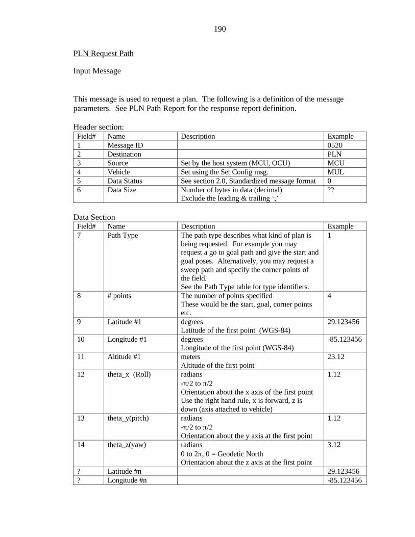
190
PLN Request Path
Input Message This message is used to request a plan. The following is a definition of the message parameters. See PLN Path Report for the response report definition. Header section: Field# Name Description Example 1 Message ID 0520 2 Destination PLN 3 Source Set by the host system (MCU, OCU) MCU 4 Vehicle Set using the Set Config msg. MUL 5 Data Status See section 2.0, Standardized message format 0 6 Data Size Number of bytes in data (decimal)
Exclude the leading & trailing ‘,’ ??
Data Section
Field# Name Description Example 7 Path Type The path type describes what kind of plan is
being requested. For example you may request a go to goal path and give the start and goal poses. Alternatively, you may request a sweep path and specify the corner points of the field. See the Path Type table for type identifiers.
1
8 # points The number of points specified These would be the start, goal, corner points etc.
4
9 Latitude #1 degrees Latitude of the first point (WGS-84)
29.123456
10 Longitude #1 degrees Longitude of the first point (WGS-84)
-85.123456
11 Altitude #1 meters Altitude of the first point
23.12
12 theta_x (Roll) radians -π/2 to π/2 Orientation about the x axis of the first point Use the right hand rule, x is forward, z is down (axis attached to vehicle)
1.12
13 theta_y(pitch) radians -π/2 to π/2 Orientation about the y axis at the first point
1.12
14 theta_z(yaw) radians 0 to 2π, 0 = Geodetic North Orientation about the z axis at the first point
3.12
? Latitude #n 29.123456 ? Longitude #n -85.123456

191
? Altitude #n 23.12 ? theta_x (Roll) 1.12 ? theta_y(pitch) 1.12 ? theta_z(yaw) 3.12
Example Message: [0x05]0520,PLN,MCU,MUL,0,??,,1,4,29.1234567,82.1234567,23.12,1.12,1.12,3.12....29.1234567... ,?[x03] Path Type Table
Path Type # Description Required Information 0 1 Go to Goal Start Position, Goal Position 2 3 4 5 Field Sweep Corner points of field

192
PLN Path Report
Output Message This is the main message from the planner system. The following is a description of the parameters: Header section: Field# Name Description Example 1 Message ID 05C0 2 Destination Destination will be set equal to the source of
the Start Report message MCU
3 Source PLN 4 Vehicle Set using the Set Config msg. MUL 5 Data Status See section 2.0, Standardized message format 0 6 Data Size Variable, set prior to shipping (use sizeof()) ??
Data Section
Field# Name Description Example 7 Path Type See table of path types under PLN Request
Plan 1
8 Path Status 0=Path OK 1=Path is not valid 0 9 Path Length Meters 2500 10 # sub-goals number of sub-goals 950 11 Latitude #1 degrees
Latitude of the first point (WGS-84) 29.123456
12 Longitude #1 degrees Longitude of the first point (WGS-84)
-85.123456
13 Altitude #1 meters Altitude of the first point
23.12
14 theta_x (Roll) radians -π/2 to π/2 Orientation about the x axis of the first point Use the right hand rule, x is forward, z is down (axis attached to vehicle)
1.12
15 theta_y(pitch) radians -π/2 to π/2 Orientation about the y axis at the first point
1.12
16 theta_z(yaw) radians 0 to 2π, 0 = Geodetic North Orientation about the z axis at the first point
3.12
?? Latitude #n 29.1234567 ?? Longitude #n -85.123456 ?? Altitude #n 23.12 ?? theta_x (Roll) 1.12 ?? theta_y (pitch) 1.12 ?? theta_z (yaw) 3.12 ?? PLN Status See Below 03
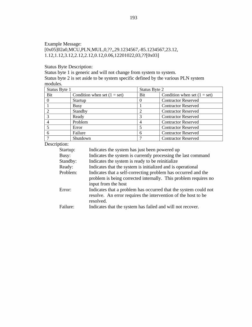
193
Example Message: [0x05]02a0,MCU,PLN,MUL,0,??,,29.1234567,-85.1234567,23.12, 1.12,1.12,3.12,2.12,2.12,0.12,0.06,12201022,03,??[0x03] Status Byte Description: Status byte 1 is generic and will not change from system to system. Status byte 2 is set aside to be system specific defined by the various PLN system modules. Status Byte 1 Status Byte 2 Bit Condition when set (1 = set) Bit Condition when set (1 = set) 0 Startup 0 Contractor Reserved 1 Busy 1 Contractor Reserved 2 Standby 2 Contractor Reserved 3 Ready 3 Contractor Reserved 4 Problem 4 Contractor Reserved 5 Error 5 Contractor Reserved 6 Failure 6 Contractor Reserved 7 Shutdown 7 Contractor Reserved
Description: Startup: Indicates the system has just been powered up Busy: Indicates the system is currently processing the last command Standby: Indicates the system is ready to be reinitialize Ready: Indicates that the system is initialized and is operational Problem: Indicates that a self-correcting problem has occurred and the
problem is being corrected internally. This problem requires no input from the host
Error: Indicates that a problem has occurred that the system could not resolve. An error requires the intervention of the host to be resolved.
Failure: Indicates that the system has failed and will not recover.

194
PLN Configuration Report
Output Message This message is used to report the current configuration of the planner system. The following is a description of the parameters: Header section: Field# Name Description Example 1 Message ID 05A2 2 Destination Destination will be set equal to the source of
the Start Report message MCU
3 Source PLN 4 Vehicle Set using the Set Config msg. MUL 5 Data Status See section 2.0, Standardized message format 0 6 Data Size Variable, set prior to shipping (use sizeof()) ??
Data Section
Field# Name Description Example 7 Text Description Free form text description. May list the main
components used by the system and or other pertinent information.
Planner System: Plans go to goal and field sweep paths
8 System Identification Gives a hex number assigned to the particular planner system so that it may be more uniquely described.
11
Example Message: [0x05]05A2,MCU,PLN,MUL,0,??,Planner System: Plans go to goal and field sweep paths,11,??[0x03]

195
PLN Status Report
Output Message Provides the host with the system status information Header section: Field# Name Description Example 1 Message ID 05A4 2 Destination Destination will be set equal to the source of
the start Report message MCU
3 Source PLN 4 Vehicle Set using the Set Config msg. MUL 5 Data Status See section 2.0, Standardized message format 0 6 Data Size Number of bytes in data (decimal)
Exclude the leading & trailing ‘,’ 8
Data Section
Field# Name Description Example 7 Status 4 bytes: See Below 01
Example Message: [0x05]02a4,MCU,PLN,MUL,0,8,01,??[0x03] 7. See PLN Report for Status Byte Description

196
APPENDIX B NTV SIMULATION RESULTS
Simulations were done by using a Silicon Graphics computer and Motif and
Inventor software libraries. The model used to determine the vehicle motion is given in
Chapter 5.
-60 -50 -40 -30 -20 -10 0 10 20-80
-70
-60
-50
-40
-30
-20
-10
0
10
East (meters)
Nor
th (
met
ers)
Planned PathActual Path
Figure B.1: Follow the Carrot at 1.5 meters per second with a 3-meter look-ahead
distance.
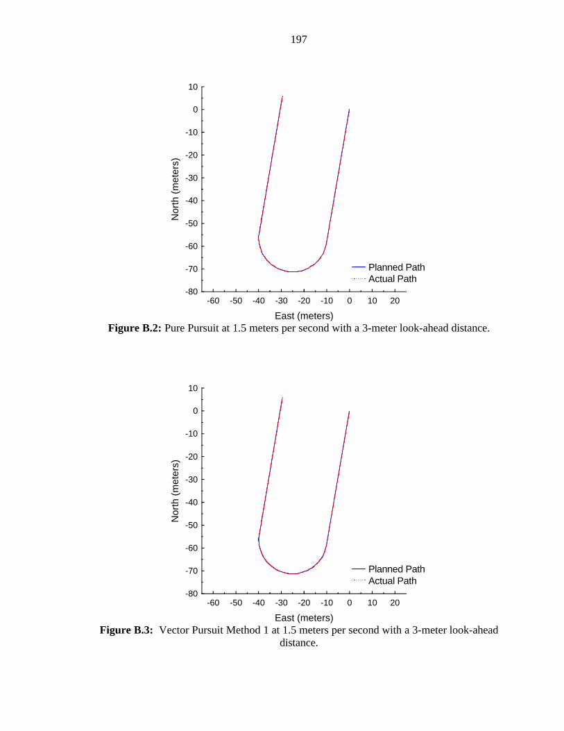
197
-60 -50 -40 -30 -20 -10 0 10 20-80
-70
-60
-50
-40
-30
-20
-10
0
10
East (meters)
Nor
th (
met
ers)
Planned PathActual Path
Figure B.2: Pure Pursuit at 1.5 meters per second with a 3-meter look-ahead distance.
-60 -50 -40 -30 -20 -10 0 10 20-80
-70
-60
-50
-40
-30
-20
-10
0
10
East (meters)
Nor
th (
met
ers)
Planned PathActual Path
Figure B.3: Vector Pursuit Method 1 at 1.5 meters per second with a 3-meter look-ahead
distance.

198
-60 -50 -40 -30 -20 -10 0 10 20-80
-70
-60
-50
-40
-30
-20
-10
0
10
East (meters)
Nor
th (
met
ers)
Planned PathActual Path
Figure B.4: Vector Pursuit Method 2 at 1.5 meters per second with a 3-meter look-ahead
distance.
-60 -50 -40 -30 -20 -10 0 10 20-80
-70
-60
-50
-40
-30
-20
-10
0
10
East (meters)
Nor
th (
met
ers)
Planned PathActual Path
Figure B.5: Follow the Carrot at 3.0 meters per second with a 5-meter look-ahead
distance.
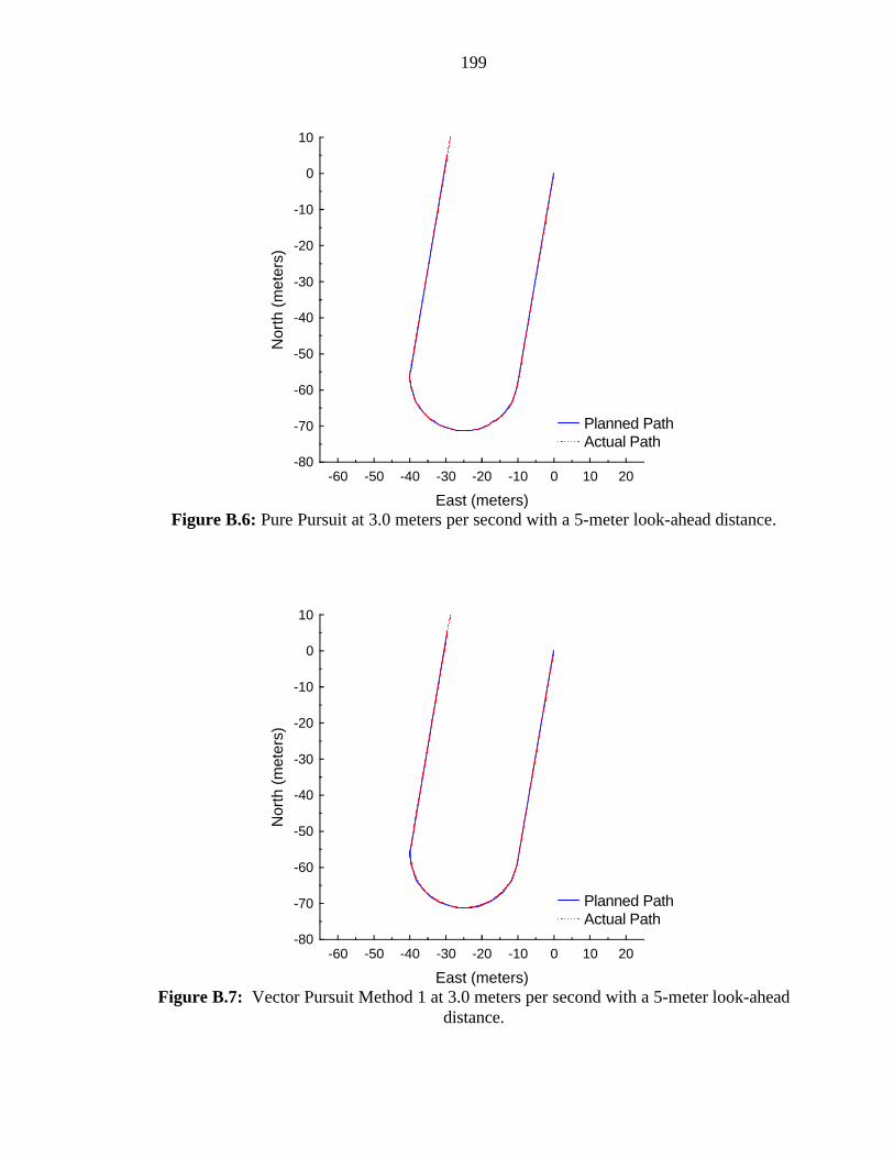
199
-60 -50 -40 -30 -20 -10 0 10 20-80
-70
-60
-50
-40
-30
-20
-10
0
10
East (meters)
Nor
th (
met
ers)
Planned PathActual Path
Figure B.6: Pure Pursuit at 3.0 meters per second with a 5-meter look-ahead distance.
-60 -50 -40 -30 -20 -10 0 10 20-80
-70
-60
-50
-40
-30
-20
-10
0
10
East (meters)
Nor
th (
met
ers)
Planned PathActual Path
Figure B.7: Vector Pursuit Method 1 at 3.0 meters per second with a 5-meter look-ahead
distance.
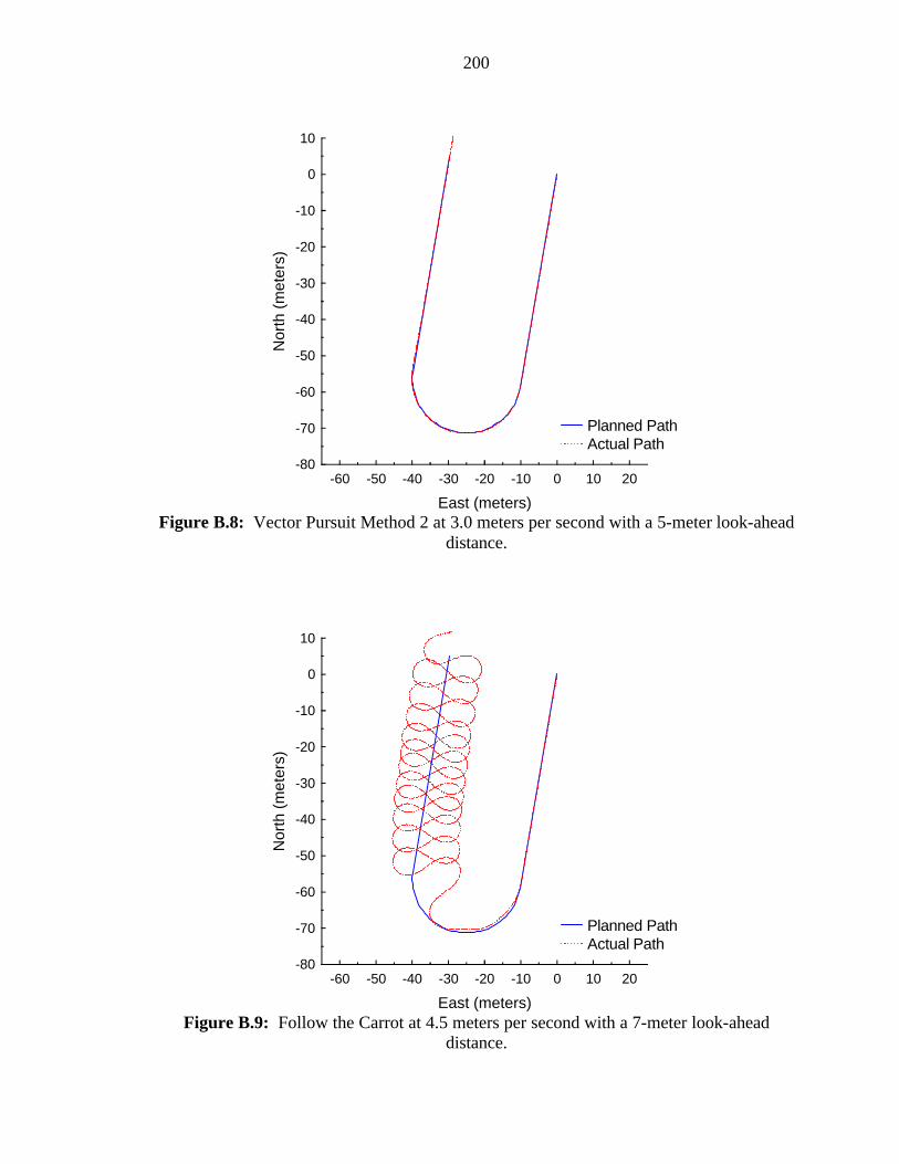
200
-60 -50 -40 -30 -20 -10 0 10 20-80
-70
-60
-50
-40
-30
-20
-10
0
10
East (meters)
Nor
th (
met
ers)
Planned PathActual Path
Figure B.8: Vector Pursuit Method 2 at 3.0 meters per second with a 5-meter look-ahead
distance.
-60 -50 -40 -30 -20 -10 0 10 20-80
-70
-60
-50
-40
-30
-20
-10
0
10
East (meters)
Nor
th (
met
ers)
Planned PathActual Path
Figure B.9: Follow the Carrot at 4.5 meters per second with a 7-meter look-ahead
distance.

201
-60 -50 -40 -30 -20 -10 0 10 20-80
-70
-60
-50
-40
-30
-20
-10
0
10
East (meters)
Nor
th (
met
ers)
Planned PathActual Path
Figure B.10: Pure Pursuit at 4.5 meters per second with a 7-meter look-ahead distance.
-60 -50 -40 -30 -20 -10 0 10 20-80
-70
-60
-50
-40
-30
-20
-10
0
10
East (meters)
Nor
th (
met
ers)
Planned PathActual Path
Figure B.11: Vector Pursuit Method 1 at 4.5 meters per second with a 7-meter look-
ahead distance.

202
-60 -50 -40 -30 -20 -10 0 10 20-80
-70
-60
-50
-40
-30
-20
-10
0
10
East (meters)
Nor
th (
met
ers)
Planned PathActual Path
Figure B.12: Vector Pursuit Method 2 at 4.5 meters per second with a 7-meter look-
ahead distance.
-40 -30 -20 -10 0 10 20 30-60
-50
-40
-30
-20
-10
0
10
East (meters)
Nor
th (
met
ers)
Planned PathActual Path
Figure B.13: Follow the Carrot at 1.5 meters per second with a 3-meter look-ahead
distance.
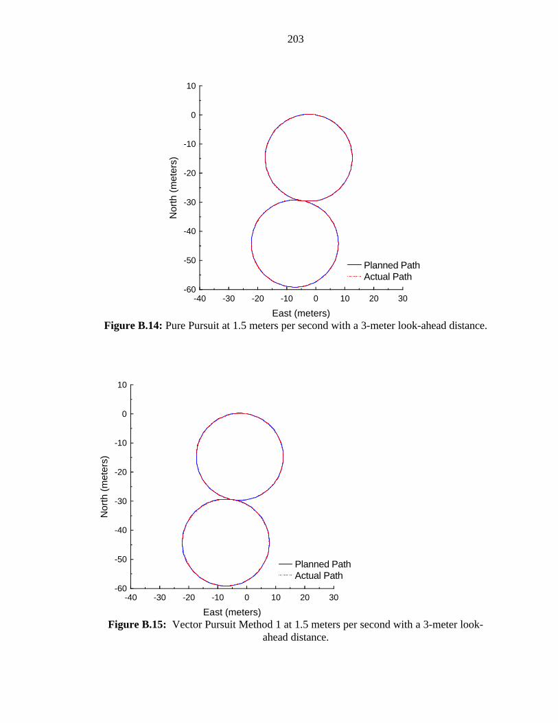
203
-40 -30 -20 -10 0 10 20 30-60
-50
-40
-30
-20
-10
0
10
East (meters)
Nor
th (
met
ers)
Planned PathActual Path
Figure B.14: Pure Pursuit at 1.5 meters per second with a 3-meter look-ahead distance.
-40 -30 -20 -10 0 10 20 30-60
-50
-40
-30
-20
-10
0
10
East (meters)
Nor
th (
met
ers)
Planned PathActual Path
Figure B.15: Vector Pursuit Method 1 at 1.5 meters per second with a 3-meter look-
ahead distance.

204
-40 -30 -20 -10 0 10 20 30-60
-50
-40
-30
-20
-10
0
10
East (meters)
Nor
th (
met
ers)
Planned PathActual Path
Figure B.16: Vector Pursuit Method 2 at 1.5 meters per second with a 3-meter look-
ahead distance.
-40 -30 -20 -10 0 10 20 30-60
-50
-40
-30
-20
-10
0
10
East (meters)
Nor
th (
met
ers)
Planned PathActual Path
Figure B.17: Follow the Carrot at 3.0 meters per second with a 5-meter look-ahead
distance.

205
-40 -30 -20 -10 0 10 20 30-60
-50
-40
-30
-20
-10
0
10
East (meters)
Nor
th (
met
ers)
Planned PathActual Path
Figure B.18: Pure Pursuit at 3.0 meters per second with a 5-meter look-ahead distance.
-40 -30 -20 -10 0 10 20 30-60
-50
-40
-30
-20
-10
0
10
East (meters)
Nor
th (
met
ers)
Planned PathActual Path
Figure B.19: Vector Pursuit Method 1 at 3.0 meters per second with a 5-meter look-
ahead distance.
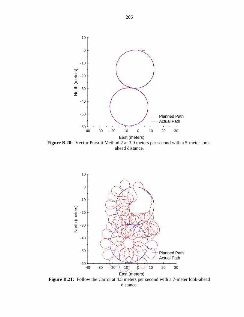
206
-40 -30 -20 -10 0 10 20 30-60
-50
-40
-30
-20
-10
0
10
East (meters)
Nor
th (
met
ers)
Planned PathActual Path
Figure B.20: Vector Pursuit Method 2 at 3.0 meters per second with a 5-meter look-
ahead distance.
-40 -30 -20 -10 0 10 20 30-60
-50
-40
-30
-20
-10
0
10
East (meters)
Nor
th (
met
ers)
Planned PathActual Path
Figure B.21: Follow the Carrot at 4.5 meters per second with a 7-meter look-ahead
distance.

207
-40 -30 -20 -10 0 10 20 30-60
-50
-40
-30
-20
-10
0
10
East (meters)
Nor
th (
met
ers)
Planned PathActual Path
Figure B.22: Pure Pursuit at 4.5 meters per second with a 7-meter look-ahead distance.
-40 -30 -20 -10 0 10 20 30-60
-50
-40
-30
-20
-10
0
10
East (meters)
Nor
th (
met
ers)
Planned PathActual Path
Figure B.23: Vector Pursuit Method 1 at 4.5 meters per second with a 7-meter look-
ahead distance.
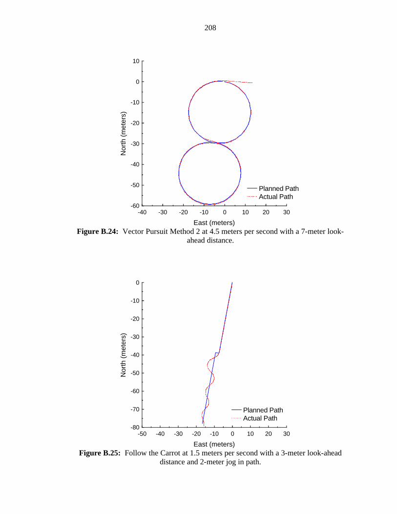
208
-40 -30 -20 -10 0 10 20 30-60
-50
-40
-30
-20
-10
0
10
East (meters)
Nor
th (
met
ers)
Planned PathActual Path
Figure B.24: Vector Pursuit Method 2 at 4.5 meters per second with a 7-meter look-
ahead distance.
-50 -40 -30 -20 -10 0 10 20 30-80
-70
-60
-50
-40
-30
-20
-10
0
East (meters)
Nor
th (
met
ers)
Planned PathActual Path
Figure B.25: Follow the Carrot at 1.5 meters per second with a 3-meter look-ahead
distance and 2-meter jog in path.
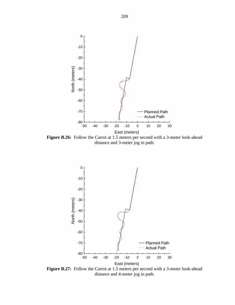
209
-50 -40 -30 -20 -10 0 10 20 30-80
-70
-60
-50
-40
-30
-20
-10
0
East (meters)
Nor
th (
met
ers)
Planned PathActual Path
Figure B.26: Follow the Carrot at 1.5 meters per second with a 3-meter look-ahead
distance and 3-meter jog in path.
-50 -40 -30 -20 -10 0 10 20 30-80
-70
-60
-50
-40
-30
-20
-10
0
East (meters)
Nor
th (
met
ers)
Planned PathActual Path
Figure B.27: Follow the Carrot at 1.5 meters per second with a 3-meter look-ahead
distance and 4-meter jog in path.
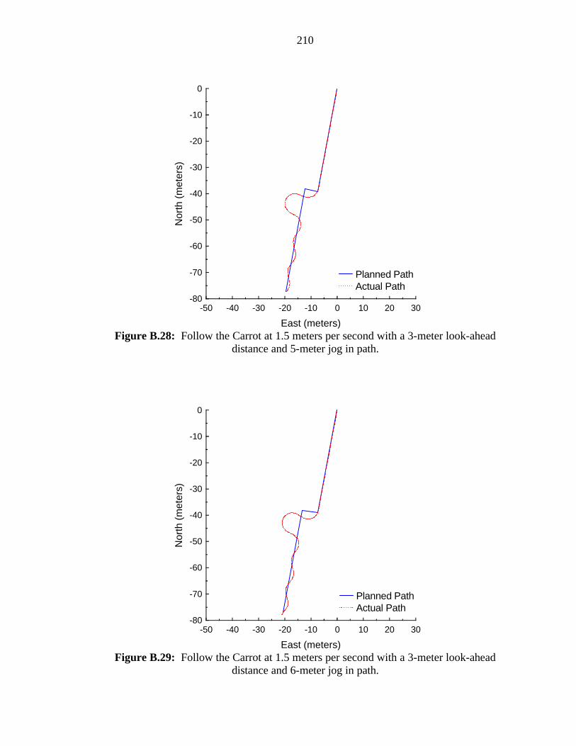
210
-50 -40 -30 -20 -10 0 10 20 30-80
-70
-60
-50
-40
-30
-20
-10
0
East (meters)
Nor
th (
met
ers)
Planned PathActual Path
Figure B.28: Follow the Carrot at 1.5 meters per second with a 3-meter look-ahead
distance and 5-meter jog in path.
-50 -40 -30 -20 -10 0 10 20 30-80
-70
-60
-50
-40
-30
-20
-10
0
East (meters)
Nor
th (
met
ers)
Planned PathActual Path
Figure B.29: Follow the Carrot at 1.5 meters per second with a 3-meter look-ahead
distance and 6-meter jog in path.
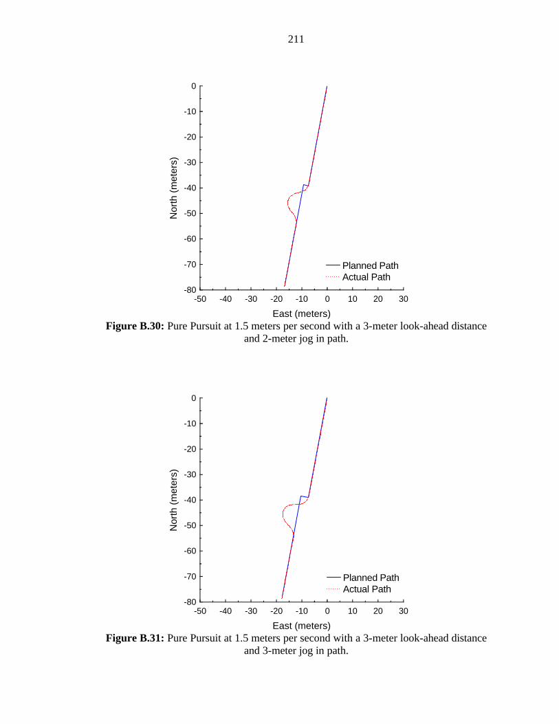
211
-50 -40 -30 -20 -10 0 10 20 30-80
-70
-60
-50
-40
-30
-20
-10
0
East (meters)
Nor
th (
met
ers)
Planned PathActual Path
Figure B.30: Pure Pursuit at 1.5 meters per second with a 3-meter look-ahead distance
and 2-meter jog in path.
-50 -40 -30 -20 -10 0 10 20 30-80
-70
-60
-50
-40
-30
-20
-10
0
East (meters)
Nor
th (
met
ers)
Planned PathActual Path
Figure B.31: Pure Pursuit at 1.5 meters per second with a 3-meter look-ahead distance
and 3-meter jog in path.
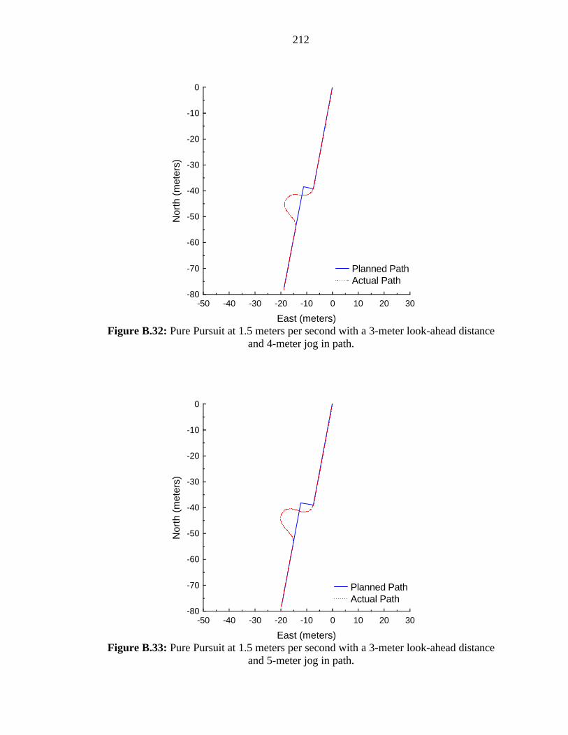
212
-50 -40 -30 -20 -10 0 10 20 30-80
-70
-60
-50
-40
-30
-20
-10
0
East (meters)
Nor
th (
met
ers)
Planned PathActual Path
Figure B.32: Pure Pursuit at 1.5 meters per second with a 3-meter look-ahead distance
and 4-meter jog in path.
-50 -40 -30 -20 -10 0 10 20 30-80
-70
-60
-50
-40
-30
-20
-10
0
East (meters)
Nor
th (
met
ers)
Planned PathActual Path
Figure B.33: Pure Pursuit at 1.5 meters per second with a 3-meter look-ahead distance
and 5-meter jog in path.
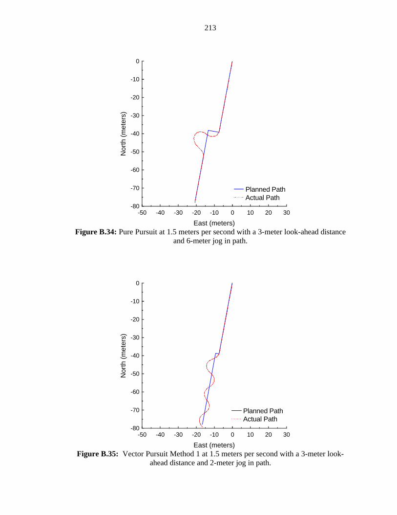
213
-50 -40 -30 -20 -10 0 10 20 30-80
-70
-60
-50
-40
-30
-20
-10
0
East (meters)
Nor
th (
met
ers)
Planned PathActual Path
Figure B.34: Pure Pursuit at 1.5 meters per second with a 3-meter look-ahead distance
and 6-meter jog in path.
-50 -40 -30 -20 -10 0 10 20 30-80
-70
-60
-50
-40
-30
-20
-10
0
East (meters)
Nor
th (
met
ers)
Planned PathActual Path
Figure B.35: Vector Pursuit Method 1 at 1.5 meters per second with a 3-meter look-
ahead distance and 2-meter jog in path.
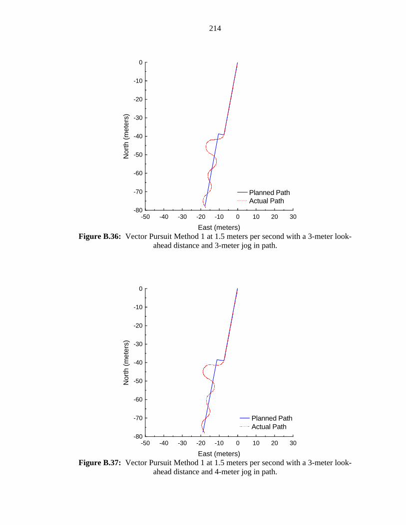
214
-50 -40 -30 -20 -10 0 10 20 30-80
-70
-60
-50
-40
-30
-20
-10
0
East (meters)
Nor
th (
met
ers)
Planned PathActual Path
Figure B.36: Vector Pursuit Method 1 at 1.5 meters per second with a 3-meter look-
ahead distance and 3-meter jog in path.
-50 -40 -30 -20 -10 0 10 20 30-80
-70
-60
-50
-40
-30
-20
-10
0
East (meters)
Nor
th (
met
ers)
Planned PathActual Path
Figure B.37: Vector Pursuit Method 1 at 1.5 meters per second with a 3-meter look-
ahead distance and 4-meter jog in path.
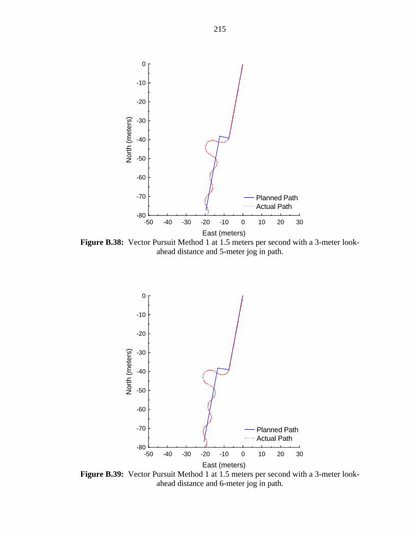
215
-50 -40 -30 -20 -10 0 10 20 30-80
-70
-60
-50
-40
-30
-20
-10
0
East (meters)
Nor
th (
met
ers)
Planned PathActual Path
Figure B.38: Vector Pursuit Method 1 at 1.5 meters per second with a 3-meter look-
ahead distance and 5-meter jog in path.
-50 -40 -30 -20 -10 0 10 20 30-80
-70
-60
-50
-40
-30
-20
-10
0
East (meters)
Nor
th (
met
ers)
Planned PathActual Path
Figure B.39: Vector Pursuit Method 1 at 1.5 meters per second with a 3-meter look-
ahead distance and 6-meter jog in path.
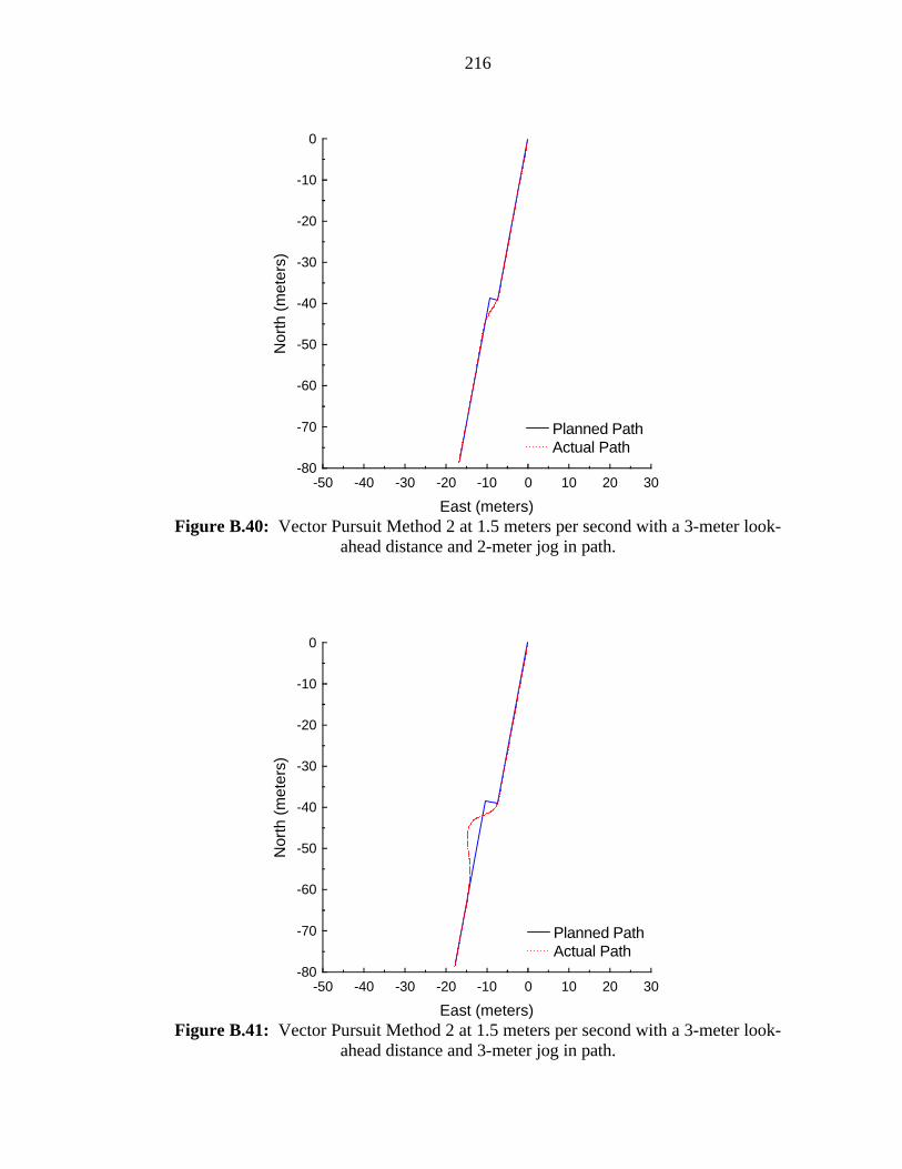
216
-50 -40 -30 -20 -10 0 10 20 30-80
-70
-60
-50
-40
-30
-20
-10
0
East (meters)
Nor
th (
met
ers)
Planned PathActual Path
Figure B.40: Vector Pursuit Method 2 at 1.5 meters per second with a 3-meter look-
ahead distance and 2-meter jog in path.
-50 -40 -30 -20 -10 0 10 20 30-80
-70
-60
-50
-40
-30
-20
-10
0
East (meters)
Nor
th (
met
ers)
Planned PathActual Path
Figure B.41: Vector Pursuit Method 2 at 1.5 meters per second with a 3-meter look-
ahead distance and 3-meter jog in path.

217
-50 -40 -30 -20 -10 0 10 20 30-80
-70
-60
-50
-40
-30
-20
-10
0
East (meters)
Nor
th (
met
ers)
Planned PathActual Path
Figure B.42: Vector Pursuit Method 2 at 1.5 meters per second with a 3-meter look-
ahead distance and 4-meter jog in path.
-50 -40 -30 -20 -10 0 10 20 30-80
-70
-60
-50
-40
-30
-20
-10
0
East (meters)
Nor
th (
met
ers)
Planned PathActual Path
Figure B.43: Vector Pursuit Method 2 at 1.5 meters per second with a 3-meter look-
ahead distance and 5-meter jog in path.

218
-50 -40 -30 -20 -10 0 10 20 30-80
-70
-60
-50
-40
-30
-20
-10
0
East (meters)
Nor
th (
met
ers)
Planned PathActual Path
Figure B.44: Vector Pursuit Method 2 at 1.5 meters per second with a 3-meter look-
ahead distance and 6-meter jog in path.
-50 -40 -30 -20 -10 0 10 20 30-80
-70
-60
-50
-40
-30
-20
-10
0
East (meters)
Nor
th (
met
ers)
Planned PathActual Path
Figure B.45: Follow the Carrot at 3.0 meters per second with a 5-meter look-ahead
distance and 2-meter jog in path.
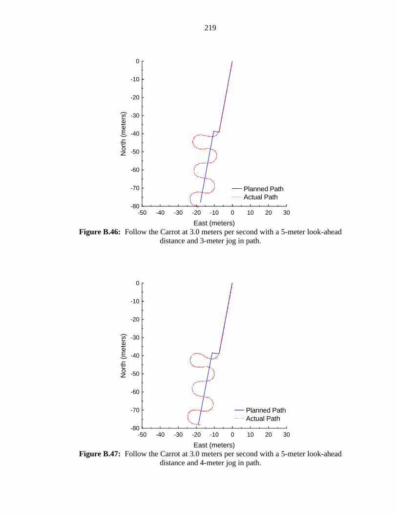
219
-50 -40 -30 -20 -10 0 10 20 30-80
-70
-60
-50
-40
-30
-20
-10
0
East (meters)
Nor
th (
met
ers)
Planned PathActual Path
Figure B.46: Follow the Carrot at 3.0 meters per second with a 5-meter look-ahead
distance and 3-meter jog in path.
-50 -40 -30 -20 -10 0 10 20 30-80
-70
-60
-50
-40
-30
-20
-10
0
East (meters)
Nor
th (
met
ers)
Planned PathActual Path
Figure B.47: Follow the Carrot at 3.0 meters per second with a 5-meter look-ahead
distance and 4-meter jog in path.

220
-50 -40 -30 -20 -10 0 10 20 30-80
-70
-60
-50
-40
-30
-20
-10
0
East (meters)
Nor
th (
met
ers)
Planned PathActual Path
Figure B.48: Follow the Carrot at 3.0 meters per second with a 5-meter look-ahead
distance and 5-meter jog in path.
-50 -40 -30 -20 -10 0 10 20 30-80
-70
-60
-50
-40
-30
-20
-10
0
East (meters)
Nor
th (
met
ers)
Planned PathActual Path
Figure B.49: Follow the Carrot at 3.0 meters per second with a 5-meter look-ahead
distance and 6-meter jog in path.
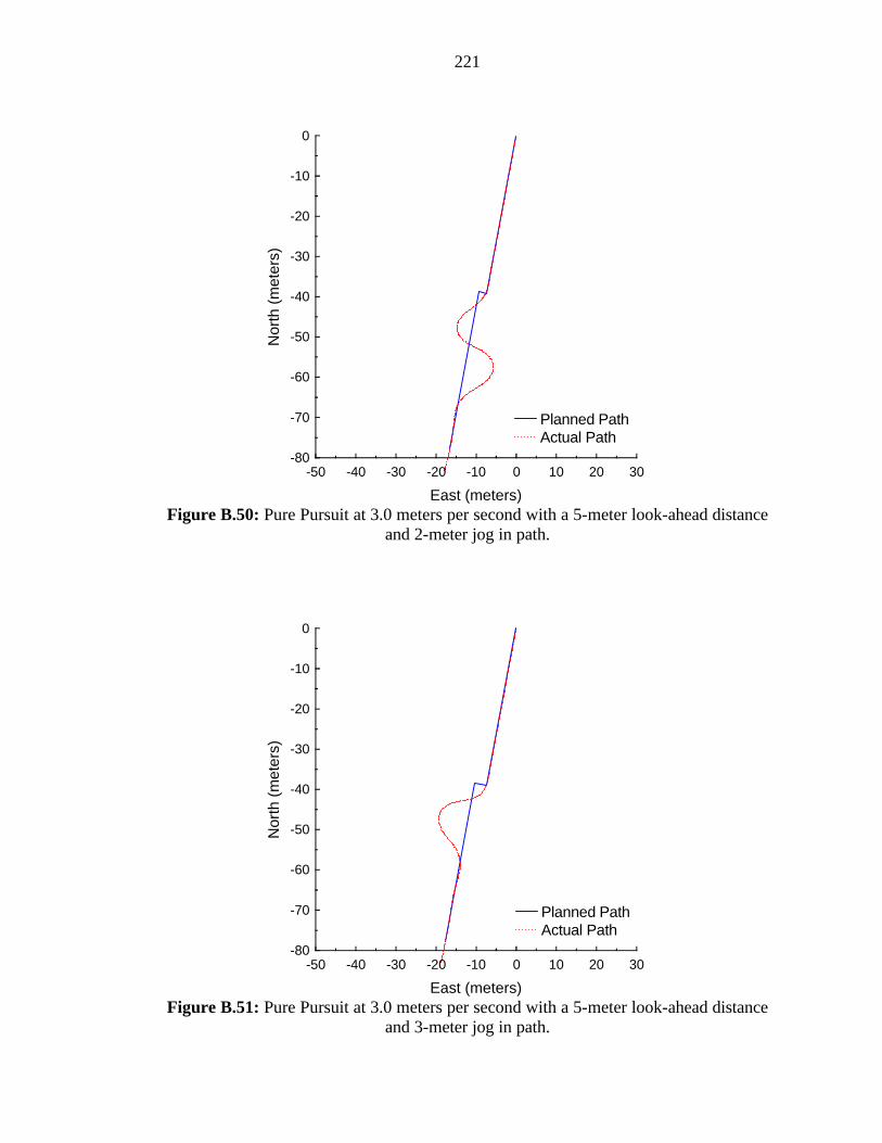
221
-50 -40 -30 -20 -10 0 10 20 30-80
-70
-60
-50
-40
-30
-20
-10
0
East (meters)
Nor
th (
met
ers)
Planned PathActual Path
Figure B.50: Pure Pursuit at 3.0 meters per second with a 5-meter look-ahead distance
and 2-meter jog in path.
-50 -40 -30 -20 -10 0 10 20 30-80
-70
-60
-50
-40
-30
-20
-10
0
East (meters)
Nor
th (
met
ers)
Planned PathActual Path
Figure B.51: Pure Pursuit at 3.0 meters per second with a 5-meter look-ahead distance
and 3-meter jog in path.
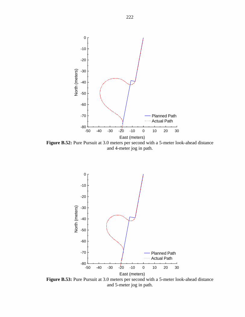
222
-50 -40 -30 -20 -10 0 10 20 30-80
-70
-60
-50
-40
-30
-20
-10
0
East (meters)
Nor
th (
met
ers)
Planned PathActual Path
Figure B.52: Pure Pursuit at 3.0 meters per second with a 5-meter look-ahead distance
and 4-meter jog in path.
-50 -40 -30 -20 -10 0 10 20 30-80
-70
-60
-50
-40
-30
-20
-10
0
East (meters)
Nor
th (
met
ers)
Planned PathActual Path
Figure B.53: Pure Pursuit at 3.0 meters per second with a 5-meter look-ahead distance
and 5-meter jog in path.
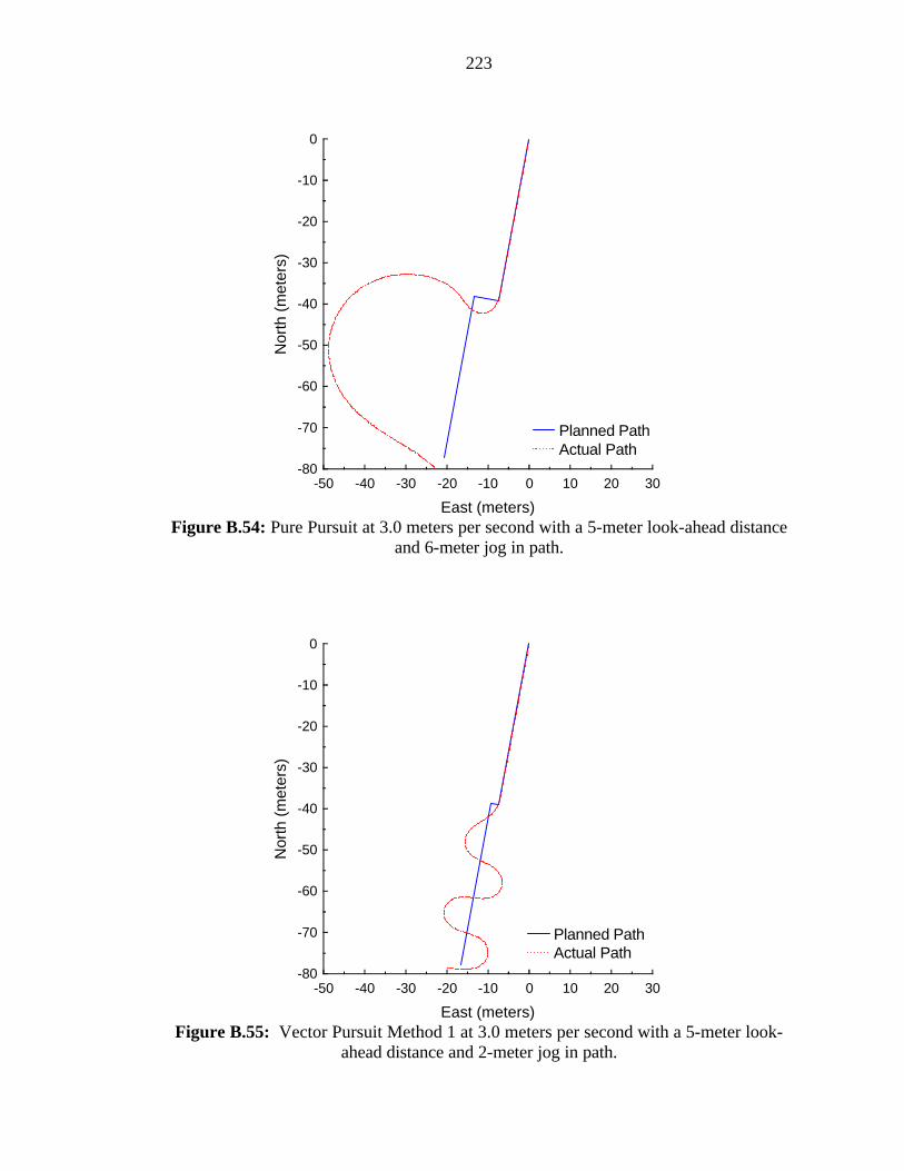
223
-50 -40 -30 -20 -10 0 10 20 30-80
-70
-60
-50
-40
-30
-20
-10
0
East (meters)
Nor
th (
met
ers)
Planned PathActual Path
Figure B.54: Pure Pursuit at 3.0 meters per second with a 5-meter look-ahead distance
and 6-meter jog in path.
-50 -40 -30 -20 -10 0 10 20 30-80
-70
-60
-50
-40
-30
-20
-10
0
East (meters)
Nor
th (
met
ers)
Planned PathActual Path
Figure B.55: Vector Pursuit Method 1 at 3.0 meters per second with a 5-meter look-
ahead distance and 2-meter jog in path.
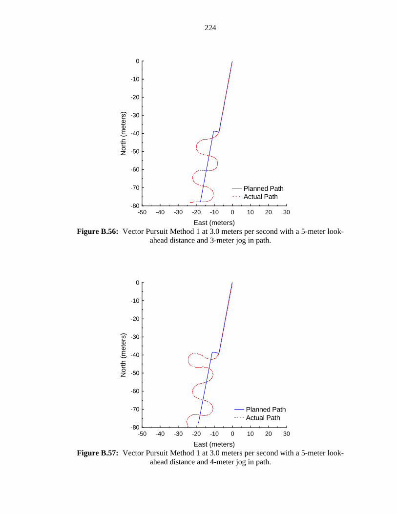
224
-50 -40 -30 -20 -10 0 10 20 30-80
-70
-60
-50
-40
-30
-20
-10
0
East (meters)
Nor
th (
met
ers)
Planned PathActual Path
Figure B.56: Vector Pursuit Method 1 at 3.0 meters per second with a 5-meter look-
ahead distance and 3-meter jog in path.
-50 -40 -30 -20 -10 0 10 20 30-80
-70
-60
-50
-40
-30
-20
-10
0
East (meters)
Nor
th (
met
ers)
Planned PathActual Path
Figure B.57: Vector Pursuit Method 1 at 3.0 meters per second with a 5-meter look-
ahead distance and 4-meter jog in path.
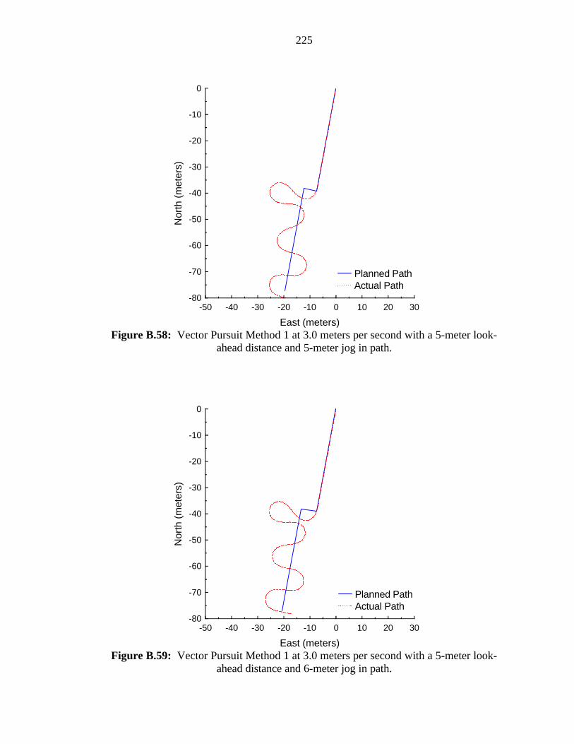
225
-50 -40 -30 -20 -10 0 10 20 30-80
-70
-60
-50
-40
-30
-20
-10
0
East (meters)
Nor
th (
met
ers)
Planned PathActual Path
Figure B.58: Vector Pursuit Method 1 at 3.0 meters per second with a 5-meter look-
ahead distance and 5-meter jog in path.
-50 -40 -30 -20 -10 0 10 20 30-80
-70
-60
-50
-40
-30
-20
-10
0
East (meters)
Nor
th (
met
ers)
Planned PathActual Path
Figure B.59: Vector Pursuit Method 1 at 3.0 meters per second with a 5-meter look-
ahead distance and 6-meter jog in path.

226
-50 -40 -30 -20 -10 0 10 20 30-80
-70
-60
-50
-40
-30
-20
-10
0
East (meters)
Nor
th (
met
ers)
Planned PathActual Path
Figure B.60: Vector Pursuit Method 2 at 3.0 meters per second with a 5-meter look-
ahead distance and 2-meter jog in path.
-50 -40 -30 -20 -10 0 10 20 30-80
-70
-60
-50
-40
-30
-20
-10
0
East (meters)
Nor
th (
met
ers)
Planned PathActual Path
Figure B.61: Vector Pursuit Method 2 at 3.0 meters per second with a 5-meter look-
ahead distance and 3-meter jog in path.
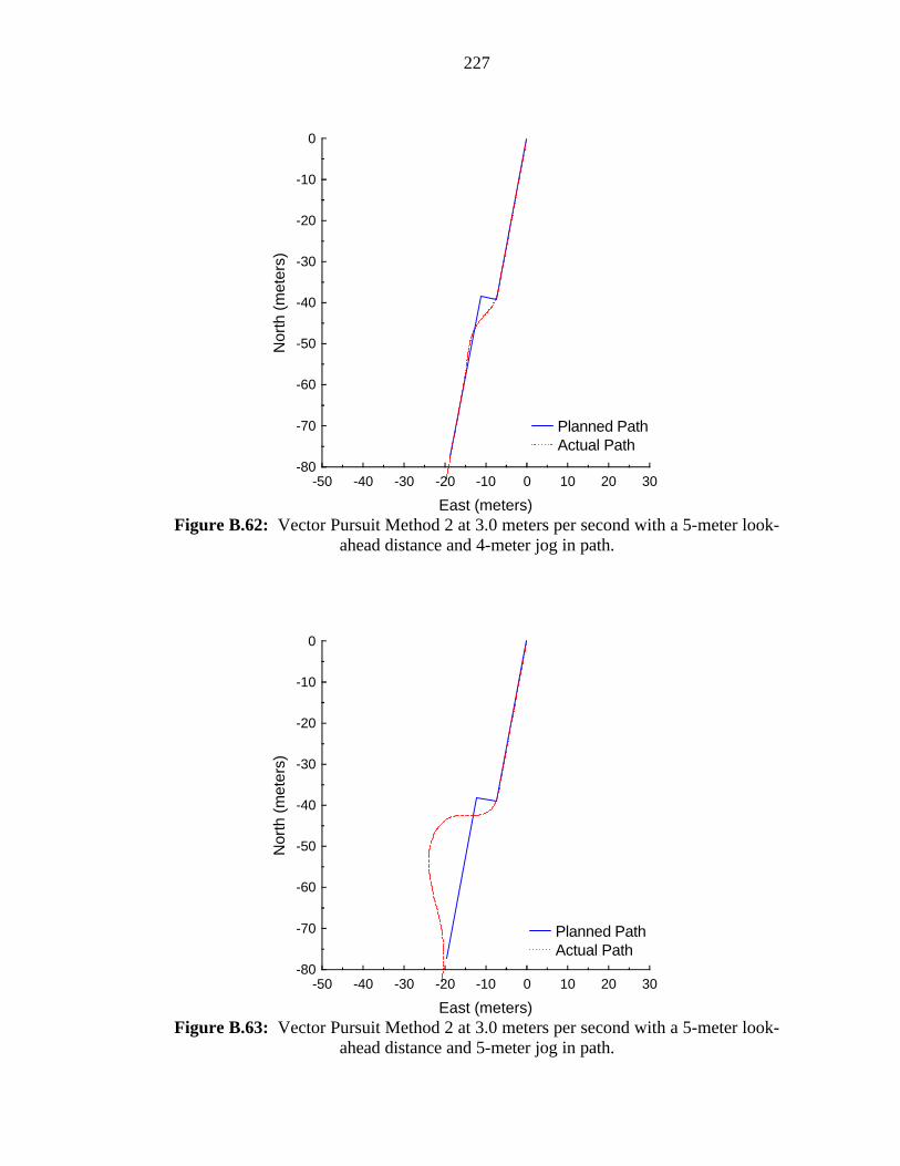
227
-50 -40 -30 -20 -10 0 10 20 30-80
-70
-60
-50
-40
-30
-20
-10
0
East (meters)
Nor
th (
met
ers)
Planned PathActual Path
Figure B.62: Vector Pursuit Method 2 at 3.0 meters per second with a 5-meter look-
ahead distance and 4-meter jog in path.
-50 -40 -30 -20 -10 0 10 20 30-80
-70
-60
-50
-40
-30
-20
-10
0
East (meters)
Nor
th (
met
ers)
Planned PathActual Path
Figure B.63: Vector Pursuit Method 2 at 3.0 meters per second with a 5-meter look-
ahead distance and 5-meter jog in path.

228
-50 -40 -30 -20 -10 0 10 20 30-80
-70
-60
-50
-40
-30
-20
-10
0
East (meters)
Nor
th (
met
ers)
Planned PathActual Path
Figure B.64: Vector Pursuit Method 2 at 3.0 meters per second with a 5-meter look-
ahead distance and 6-meter jog in path.
-50 -40 -30 -20 -10 0 10 20 30-80
-70
-60
-50
-40
-30
-20
-10
0
East (meters)
Nor
th (
met
ers)
Planned PathActual Path
Figure B.65: Follow the Carrot at 4.5 meters per second with a 7-meter look-ahead
distance and 2-meter jog in path.
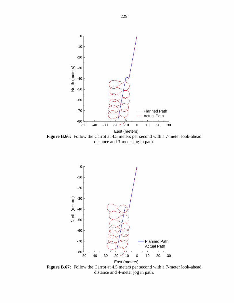
229
-50 -40 -30 -20 -10 0 10 20 30-80
-70
-60
-50
-40
-30
-20
-10
0
East (meters)
Nor
th (
met
ers)
Planned PathActual Path
Figure B.66: Follow the Carrot at 4.5 meters per second with a 7-meter look-ahead
distance and 3-meter jog in path.
-50 -40 -30 -20 -10 0 10 20 30-80
-70
-60
-50
-40
-30
-20
-10
0
East (meters)
Nor
th (
met
ers)
Planned PathActual Path
Figure B.67: Follow the Carrot at 4.5 meters per second with a 7-meter look-ahead
distance and 4-meter jog in path.
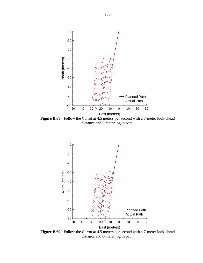
230
-50 -40 -30 -20 -10 0 10 20 30-80
-70
-60
-50
-40
-30
-20
-10
0
East (meters)
Nor
th (
met
ers)
Planned PathActual Path
Figure B.68: Follow the Carrot at 4.5 meters per second with a 7-meter look-ahead
distance and 5-meter jog in path.
-50 -40 -30 -20 -10 0 10 20 30-80
-70
-60
-50
-40
-30
-20
-10
0
East (meters)
Nor
th (
met
ers)
Planned PathActual Path
Figure B.69: Follow the Carrot at 4.5 meters per second with a 7-meter look-ahead
distance and 6-meter jog in path.

231
-50 -40 -30 -20 -10 0 10 20 30-80
-70
-60
-50
-40
-30
-20
-10
0
East (meters)
Nor
th (
met
ers)
Planned PathActual Path
Figure B.70: Pure Pursuit at 4.5 meters per second with a 7-meter look-ahead distance
and 2-meter jog in path.
-50 -40 -30 -20 -10 0 10 20 30-80
-70
-60
-50
-40
-30
-20
-10
0
East (meters)
Nor
th (
met
ers)
Planned PathActual Path
Figure B.71: Pure Pursuit at 4.5 meters per second with a 7-meter look-ahead distance
and 3-meter jog in path.

232
-50 -40 -30 -20 -10 0 10 20 30-80
-70
-60
-50
-40
-30
-20
-10
0
East (meters)
Nor
th (
met
ers)
Planned PathActual Path
Figure B.72: Pure Pursuit at 4.5 meters per second with a 7-meter look-ahead distance
and 4-meter jog in path.
-50 -40 -30 -20 -10 0 10 20 30-80
-70
-60
-50
-40
-30
-20
-10
0
East (meters)
Nor
th (
met
ers)
Planned PathActual Path
Figure B.73: Pure Pursuit at 4.5 meters per second with a 7-meter look-ahead distance
and 5-meter jog in path.

233
-50 -40 -30 -20 -10 0 10 20 30-80
-70
-60
-50
-40
-30
-20
-10
0
East (meters)
Nor
th (
met
ers)
Planned PathActual Path
Figure B.74: Pure Pursuit at 4.5 meters per second with a 7-meter look-ahead distance
and 6-meter jog in path.
-50 -40 -30 -20 -10 0 10 20 30-80
-70
-60
-50
-40
-30
-20
-10
0
East (meters)
Nor
th (
met
ers)
Planned PathActual Path
Figure B.75: Vector Pursuit Method 1 at 4.5 meters per second with a 7-meter look-
ahead distance and 2-meter jog in path.
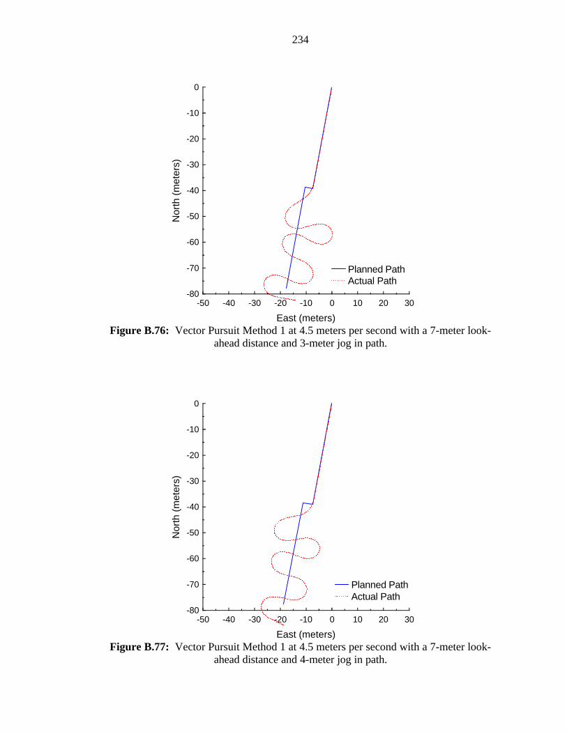
234
-50 -40 -30 -20 -10 0 10 20 30-80
-70
-60
-50
-40
-30
-20
-10
0
East (meters)
Nor
th (
met
ers)
Planned PathActual Path
Figure B.76: Vector Pursuit Method 1 at 4.5 meters per second with a 7-meter look-
ahead distance and 3-meter jog in path.
-50 -40 -30 -20 -10 0 10 20 30-80
-70
-60
-50
-40
-30
-20
-10
0
East (meters)
Nor
th (
met
ers)
Planned PathActual Path
Figure B.77: Vector Pursuit Method 1 at 4.5 meters per second with a 7-meter look-
ahead distance and 4-meter jog in path.
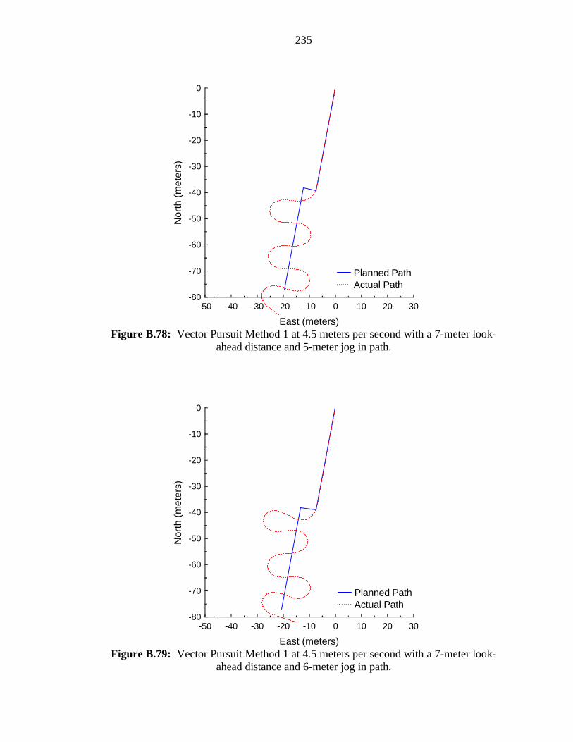
235
-50 -40 -30 -20 -10 0 10 20 30-80
-70
-60
-50
-40
-30
-20
-10
0
East (meters)
Nor
th (
met
ers)
Planned PathActual Path
Figure B.78: Vector Pursuit Method 1 at 4.5 meters per second with a 7-meter look-
ahead distance and 5-meter jog in path.
-50 -40 -30 -20 -10 0 10 20 30-80
-70
-60
-50
-40
-30
-20
-10
0
East (meters)
Nor
th (
met
ers)
Planned PathActual Path
Figure B.79: Vector Pursuit Method 1 at 4.5 meters per second with a 7-meter look-
ahead distance and 6-meter jog in path.
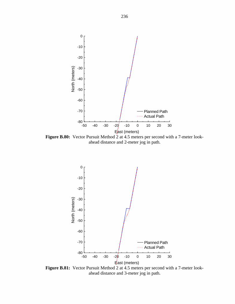
236
-50 -40 -30 -20 -10 0 10 20 30-80
-70
-60
-50
-40
-30
-20
-10
0
East (meters)
Nor
th (
met
ers)
Planned PathActual Path
Figure B.80: Vector Pursuit Method 2 at 4.5 meters per second with a 7-meter look-
ahead distance and 2-meter jog in path.
-50 -40 -30 -20 -10 0 10 20 30-80
-70
-60
-50
-40
-30
-20
-10
0
East (meters)
Nor
th (
met
ers)
Planned PathActual Path
Figure B.81: Vector Pursuit Method 2 at 4.5 meters per second with a 7-meter look-
ahead distance and 3-meter jog in path.

237
-50 -40 -30 -20 -10 0 10 20 30-80
-70
-60
-50
-40
-30
-20
-10
0
East (meters)
Nor
th (
met
ers)
Planned PathActual Path
Figure B.82: Vector Pursuit Method 2 at 4.5 meters per second with a 7-meter look-
ahead distance and 4-meter jog in path.
-50 -40 -30 -20 -10 0 10 20 30-80
-70
-60
-50
-40
-30
-20
-10
0
East (meters)
Nor
th (
met
ers)
Planned PathActual Path
Figure B.83: Vector Pursuit Method 2 at 4.5 meters per second with a 7-meter look-
ahead distance and 5-meter jog in path.

238
-50 -40 -30 -20 -10 0 10 20 30-80
-70
-60
-50
-40
-30
-20
-10
0
East (meters)
Nor
th (
met
ers)
Planned PathActual Path
Figure B.84: Vector Pursuit Method 2 at 4.5 meters per second with a 7-meter look-
ahead distance and 6-meter jog in path.
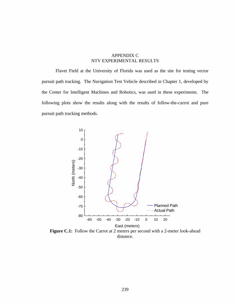
239
APPENDIX C NTV EXPERIMENTAL RESULTS
Flavet Field at the University of Florida was used as the site for testing vector
pursuit path tracking. The Navigation Test Vehicle described in Chapter 1, developed by
the Center for Intelligent Machines and Robotics, was used in these experiments. The
following plots show the results along with the results of follow-the-carrot and pure
pursuit path tracking methods.
-60 -50 -40 -30 -20 -10 0 10 20-80
-70
-60
-50
-40
-30
-20
-10
0
10
East (meters)
Nor
th (
met
ers)
Planned PathActual Path
Figure C.1: Follow the Carrot at 2 meters per second with a 2-meter look-ahead
distance.

240
-60 -50 -40 -30 -20 -10 0 10 20-80
-70
-60
-50
-40
-30
-20
-10
0
10
East (meters)
Nor
th (
met
ers)
Planned PathActual Path
Figure C.2: Follow the Carrot at 2 meters per second with a 3-meter look-ahead
distance.
-60 -50 -40 -30 -20 -10 0 10 20-80
-70
-60
-50
-40
-30
-20
-10
0
10
East (meters)
Nor
th (
met
ers)
Planned PathActual Path
Figure C.3: Follow the Carrot at 2 meters per second with a 4-meter look-ahead
distance.
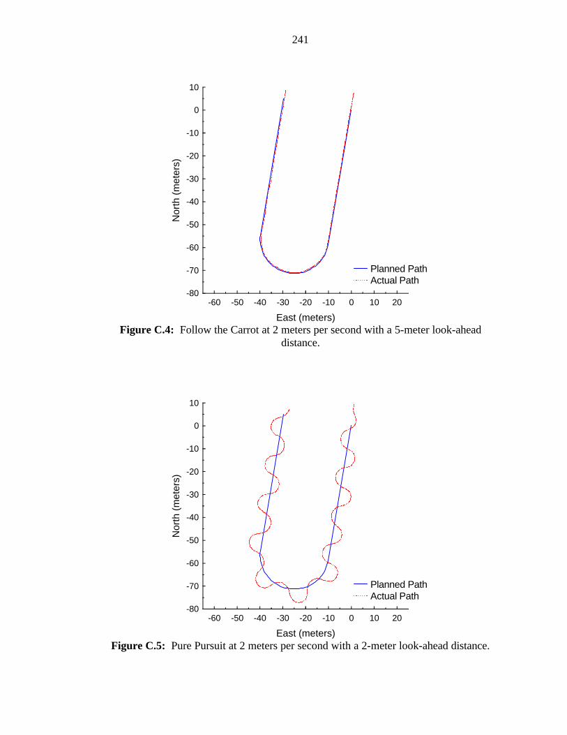
241
-60 -50 -40 -30 -20 -10 0 10 20-80
-70
-60
-50
-40
-30
-20
-10
0
10
East (meters)
Nor
th (
met
ers)
Planned PathActual Path
Figure C.4: Follow the Carrot at 2 meters per second with a 5-meter look-ahead
distance.
-60 -50 -40 -30 -20 -10 0 10 20-80
-70
-60
-50
-40
-30
-20
-10
0
10
East (meters)
Nor
th (
met
ers)
Planned PathActual Path
Figure C.5: Pure Pursuit at 2 meters per second with a 2-meter look-ahead distance.

242
-60 -50 -40 -30 -20 -10 0 10 20-80
-70
-60
-50
-40
-30
-20
-10
0
10
East (meters)
Nor
th (
met
ers)
Planned PathActual Path
Figure C.6: Pure Pursuit at 2 meters per second with a 3-meter look-ahead distance.
-60 -50 -40 -30 -20 -10 0 10 20-80
-70
-60
-50
-40
-30
-20
-10
0
10
East (meters)
Nor
th (
met
ers)
Planned PathActual Path
Figure C.7: Pure Pursuit at 2 meters per second with a 4-meter look-ahead distance.
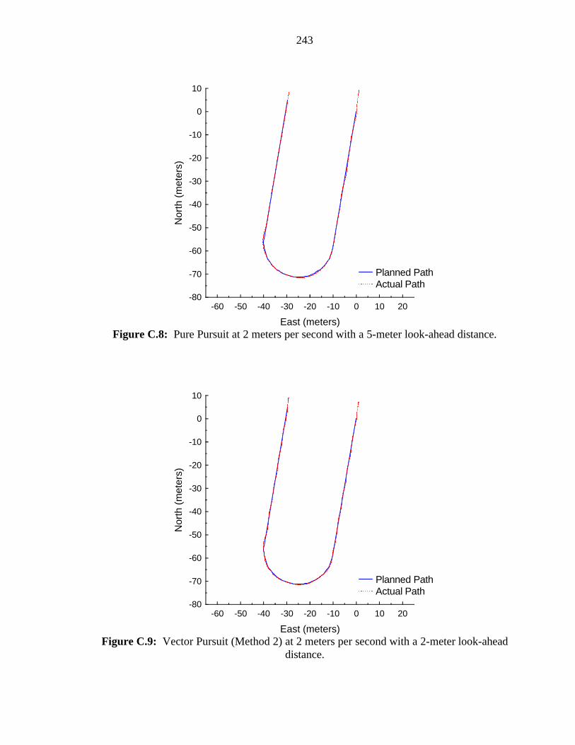
243
-60 -50 -40 -30 -20 -10 0 10 20-80
-70
-60
-50
-40
-30
-20
-10
0
10
East (meters)
Nor
th (
met
ers)
Planned PathActual Path
Figure C.8: Pure Pursuit at 2 meters per second with a 5-meter look-ahead distance.
-60 -50 -40 -30 -20 -10 0 10 20-80
-70
-60
-50
-40
-30
-20
-10
0
10
East (meters)
Nor
th (
met
ers)
Planned PathActual Path
Figure C.9: Vector Pursuit (Method 2) at 2 meters per second with a 2-meter look-ahead
distance.

244
-60 -50 -40 -30 -20 -10 0 10 20-80
-70
-60
-50
-40
-30
-20
-10
0
10
East (meters)
Nor
th (
met
ers)
Planned PathActual Path
Figure C.10: Vector Pursuit (Method 2) at 2 meters per second with a 3-meter look-
ahead distance.
-60 -50 -40 -30 -20 -10 0 10 20-80
-70
-60
-50
-40
-30
-20
-10
0
10
East (meters)
Nor
th (
met
ers)
Planned PathActual Path
Figure C.11: Vector Pursuit (Method 2) at 2 meters per second with a 4-meter look-
ahead distance.

245
-60 -50 -40 -30 -20 -10 0 10 20-80
-70
-60
-50
-40
-30
-20
-10
0
10
East (meters)
Nor
th (
met
ers)
Planned PathActual Path
Figure C.12: Vector Pursuit (Method 2) at 2 meters per second with a 5-meter look-
ahead distance.
-60 -50 -40 -30 -20 -10 0 10 20-80
-70
-60
-50
-40
-30
-20
-10
0
10
East (meters)
Nor
th (
met
ers)
Planned PathActual Path
Figure C.13: Follow the Carrot at 3 meters per second with a 4-meter look-ahead
distance.
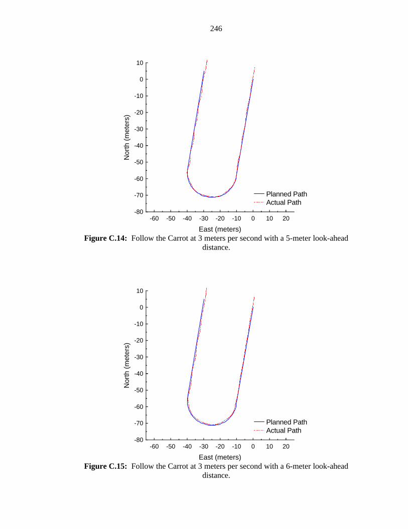
246
-60 -50 -40 -30 -20 -10 0 10 20-80
-70
-60
-50
-40
-30
-20
-10
0
10
East (meters)
Nor
th (
met
ers)
Planned PathActual Path
Figure C.14: Follow the Carrot at 3 meters per second with a 5-meter look-ahead
distance.
-60 -50 -40 -30 -20 -10 0 10 20-80
-70
-60
-50
-40
-30
-20
-10
0
10
East (meters)
Nor
th (
met
ers)
Planned PathActual Path
Figure C.15: Follow the Carrot at 3 meters per second with a 6-meter look-ahead
distance.
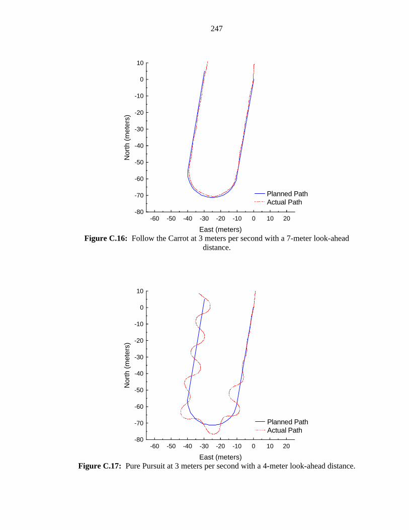
247
-60 -50 -40 -30 -20 -10 0 10 20-80
-70
-60
-50
-40
-30
-20
-10
0
10
East (meters)
Nor
th (
met
ers)
Planned PathActual Path
Figure C.16: Follow the Carrot at 3 meters per second with a 7-meter look-ahead
distance.
-60 -50 -40 -30 -20 -10 0 10 20-80
-70
-60
-50
-40
-30
-20
-10
0
10
East (meters)
Nor
th (
met
ers)
Planned PathActual Path
Figure C.17: Pure Pursuit at 3 meters per second with a 4-meter look-ahead distance.
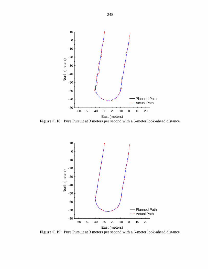
248
-60 -50 -40 -30 -20 -10 0 10 20-80
-70
-60
-50
-40
-30
-20
-10
0
10
East (meters)
Nor
th (
met
ers)
Planned PathActual Path
Figure C.18: Pure Pursuit at 3 meters per second with a 5-meter look-ahead distance.
-60 -50 -40 -30 -20 -10 0 10 20-80
-70
-60
-50
-40
-30
-20
-10
0
10
East (meters)
Nor
th (
met
ers)
Planned PathActual Path
Figure C.19: Pure Pursuit at 3 meters per second with a 6-meter look-ahead distance.
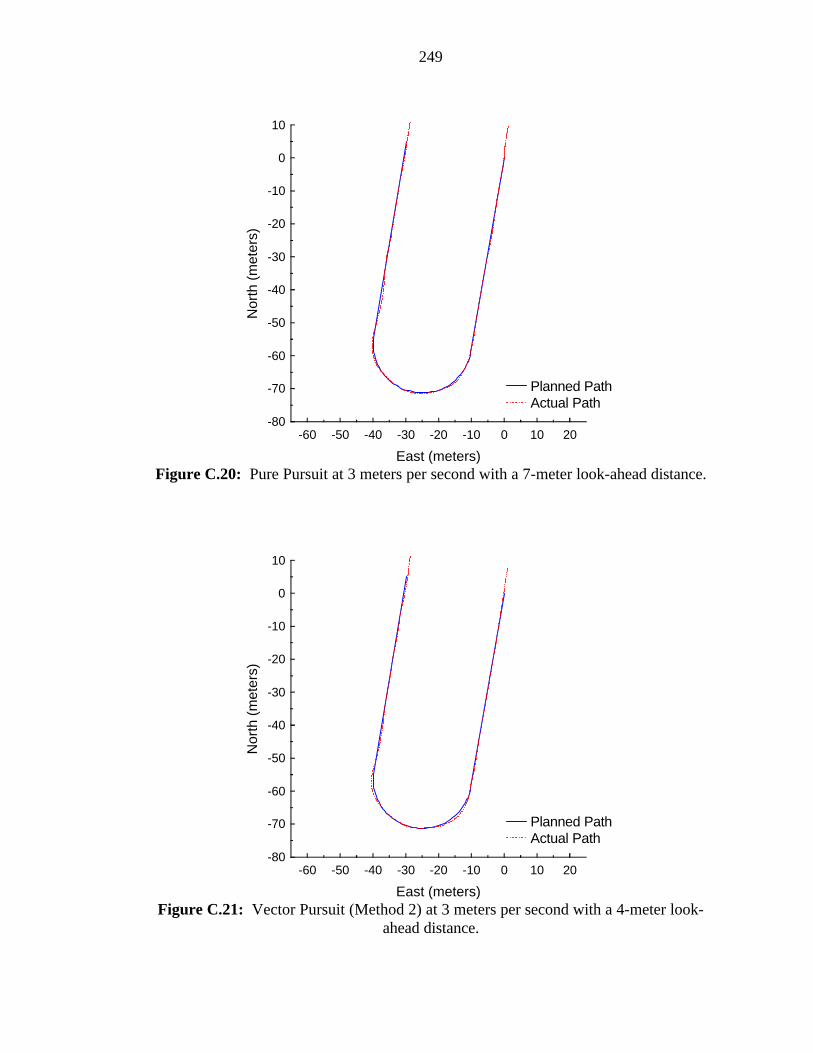
249
-60 -50 -40 -30 -20 -10 0 10 20-80
-70
-60
-50
-40
-30
-20
-10
0
10
East (meters)
Nor
th (
met
ers)
Planned PathActual Path
Figure C.20: Pure Pursuit at 3 meters per second with a 7-meter look-ahead distance.
-60 -50 -40 -30 -20 -10 0 10 20-80
-70
-60
-50
-40
-30
-20
-10
0
10
East (meters)
Nor
th (
met
ers)
Planned PathActual Path
Figure C.21: Vector Pursuit (Method 2) at 3 meters per second with a 4-meter look-
ahead distance.
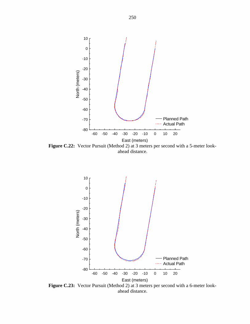
250
-60 -50 -40 -30 -20 -10 0 10 20-80
-70
-60
-50
-40
-30
-20
-10
0
10
East (meters)
Nor
th (
met
ers)
Planned PathActual Path
Figure C.22: Vector Pursuit (Method 2) at 3 meters per second with a 5-meter look-
ahead distance.
-60 -50 -40 -30 -20 -10 0 10 20-80
-70
-60
-50
-40
-30
-20
-10
0
10
East (meters)
Nor
th (
met
ers)
Planned PathActual Path
Figure C.23: Vector Pursuit (Method 2) at 3 meters per second with a 6-meter look-
ahead distance.

251
-60 -50 -40 -30 -20 -10 0 10 20-80
-70
-60
-50
-40
-30
-20
-10
0
10
East (meters)
Nor
th (
met
ers)
Planned PathActual Path
Figure C.24: Vector Pursuit (Method 2) at 3 meters per second with a 7-meter look-
ahead distance.
-60 -50 -40 -30 -20 -10 0 10 20-80
-70
-60
-50
-40
-30
-20
-10
0
10
East (meters)
Nor
th (
met
ers)
Planned PathActual Path
Figure C.25: Follow the Carrot at 4 meters per second with a 6-meter look-ahead
distance.
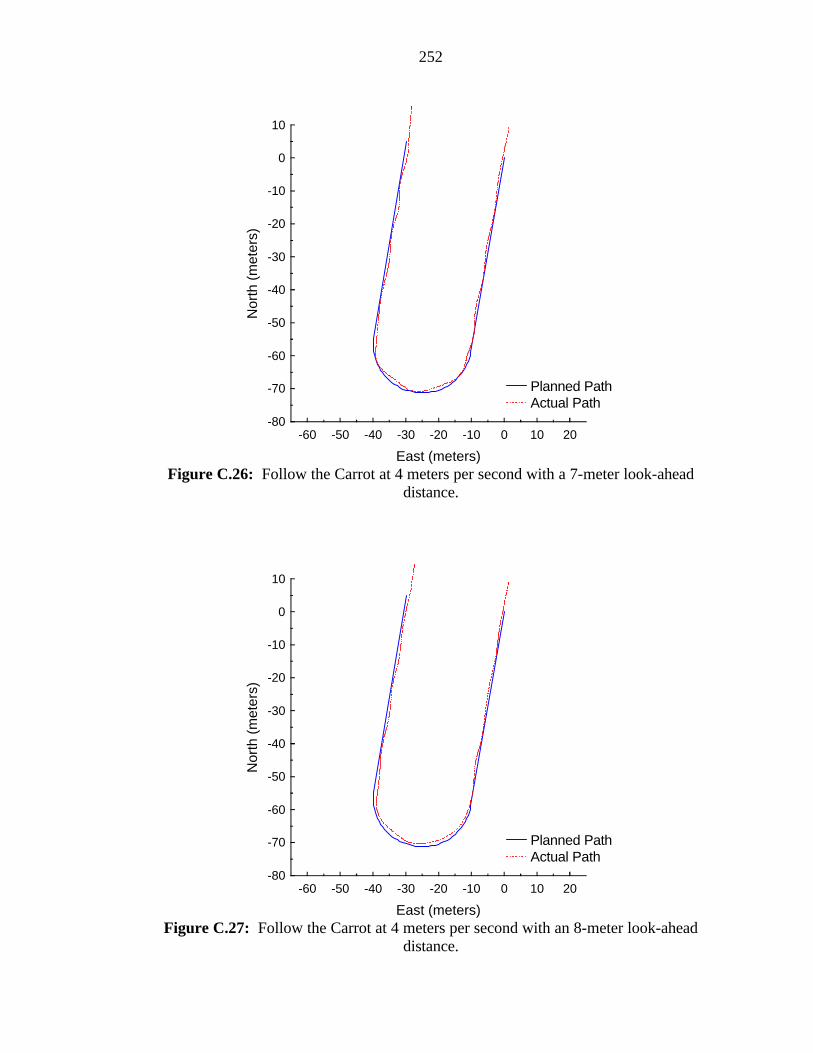
252
-60 -50 -40 -30 -20 -10 0 10 20-80
-70
-60
-50
-40
-30
-20
-10
0
10
East (meters)
Nor
th (
met
ers)
Planned PathActual Path
Figure C.26: Follow the Carrot at 4 meters per second with a 7-meter look-ahead
distance.
-60 -50 -40 -30 -20 -10 0 10 20-80
-70
-60
-50
-40
-30
-20
-10
0
10
East (meters)
Nor
th (
met
ers)
Planned PathActual Path
Figure C.27: Follow the Carrot at 4 meters per second with an 8-meter look-ahead
distance.

253
-60 -50 -40 -30 -20 -10 0 10 20-80
-70
-60
-50
-40
-30
-20
-10
0
10
East (meters)
Nor
th (
met
ers)
Planned PathActual Path
Figure C.28: Follow the Carrot at 4 meters per second with a 9-meter look-ahead
distance.
-60 -50 -40 -30 -20 -10 0 10 20-80
-70
-60
-50
-40
-30
-20
-10
0
10
East (meters)
Nor
th (
met
ers)
Planned PathActual Path
Figure C.29: Pure Pursuit at 4 meters per second with a 6-meter look-ahead distance.
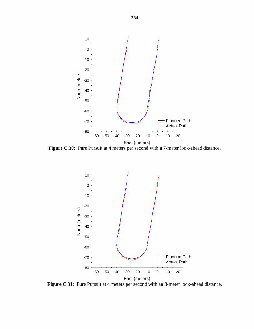
254
-60 -50 -40 -30 -20 -10 0 10 20-80
-70
-60
-50
-40
-30
-20
-10
0
10
East (meters)
Nor
th (
met
ers)
Planned PathActual Path
Figure C.30: Pure Pursuit at 4 meters per second with a 7-meter look-ahead distance.
-60 -50 -40 -30 -20 -10 0 10 20-80
-70
-60
-50
-40
-30
-20
-10
0
10
East (meters)
Nor
th (
met
ers)
Planned PathActual Path
Figure C.31: Pure Pursuit at 4 meters per second with an 8-meter look-ahead distance.
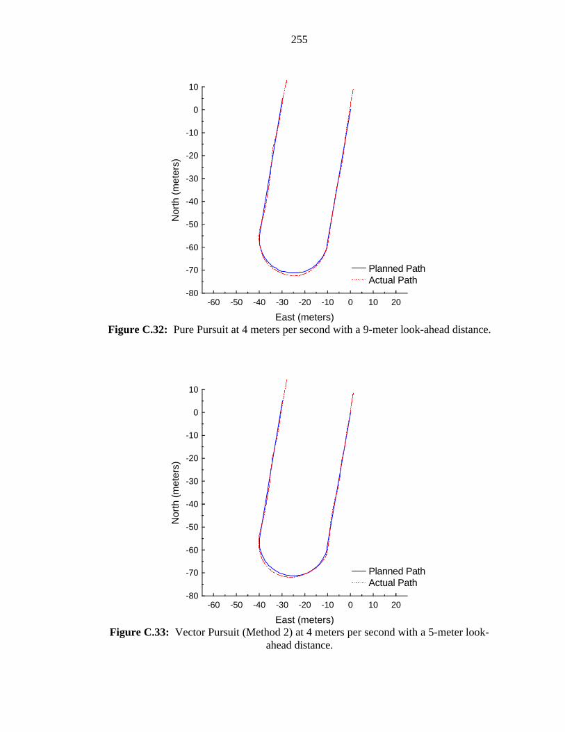
255
-60 -50 -40 -30 -20 -10 0 10 20-80
-70
-60
-50
-40
-30
-20
-10
0
10
East (meters)
Nor
th (
met
ers)
Planned PathActual Path
Figure C.32: Pure Pursuit at 4 meters per second with a 9-meter look-ahead distance.
-60 -50 -40 -30 -20 -10 0 10 20-80
-70
-60
-50
-40
-30
-20
-10
0
10
East (meters)
Nor
th (
met
ers)
Planned PathActual Path
Figure C.33: Vector Pursuit (Method 2) at 4 meters per second with a 5-meter look-
ahead distance.

256
-60 -50 -40 -30 -20 -10 0 10 20-80
-70
-60
-50
-40
-30
-20
-10
0
10
East (meters)
Nor
th (
met
ers)
Planned PathActual Path
Figure C.34: Vector Pursuit (Method 2) at 4 meters per second with a 6-meter look-
ahead distance.
-60 -50 -40 -30 -20 -10 0 10 20-80
-70
-60
-50
-40
-30
-20
-10
0
10
East (meters)
Nor
th (
met
ers)
Planned PathActual Path
Figure C.35: Vector Pursuit (Method 2) at 4 meters per second with a 7-meter look-
ahead distance.
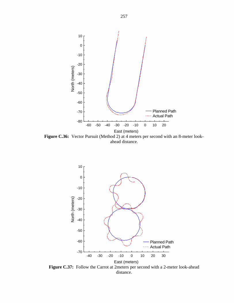
257
-60 -50 -40 -30 -20 -10 0 10 20-80
-70
-60
-50
-40
-30
-20
-10
0
10
East (meters)
Nor
th (
met
ers)
Planned PathActual Path
Figure C.36: Vector Pursuit (Method 2) at 4 meters per second with an 8-meter look-
ahead distance.
-40 -30 -20 -10 0 10 20 30-70
-60
-50
-40
-30
-20
-10
0
10
East (meters)
Nor
th (
met
ers)
Planned PathActual Path
Figure C.37: Follow the Carrot at 2meters per second with a 2-meter look-ahead
distance.

258
-40 -30 -20 -10 0 10 20 30-70
-60
-50
-40
-30
-20
-10
0
10
East (meters)
Nor
th (
met
ers)
Planned PathActual Path
Figure C.38: Follow the Carrot at 2 meters per second with a 3-meter look-ahead
distance.
-40 -30 -20 -10 0 10 20 30-70
-60
-50
-40
-30
-20
-10
0
10
East (meters)
Nor
th (
met
ers)
Planned PathActual Path
Figure C.39: Follow the Carrot at 2 meters per second with a 4-meter look-ahead
distance.

259
-40 -30 -20 -10 0 10 20 30-70
-60
-50
-40
-30
-20
-10
0
10
East (meters)
Nor
th (
met
ers)
Planned PathActual Path
Figure C.40: Follow the Carrot at 2 meters per second with a 5-meter look-ahead
distance.
-40 -30 -20 -10 0 10 20 30-70
-60
-50
-40
-30
-20
-10
0
10
East (meters)
Nor
th (
met
ers)
Planned PathActual Path
Figure C.41: Pure Pursuit at 2 meters per second with a 2-meter look-ahead distance.
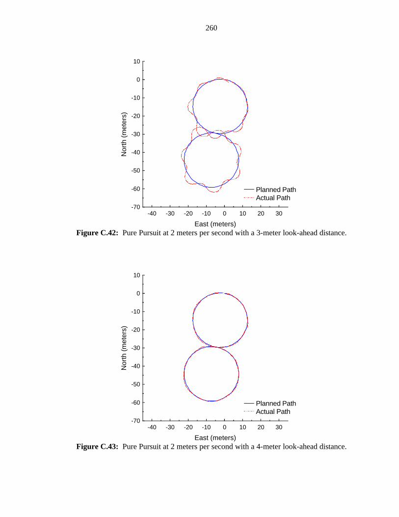
260
-40 -30 -20 -10 0 10 20 30-70
-60
-50
-40
-30
-20
-10
0
10
East (meters)
Nor
th (
met
ers)
Planned PathActual Path
Figure C.42: Pure Pursuit at 2 meters per second with a 3-meter look-ahead distance.
-40 -30 -20 -10 0 10 20 30-70
-60
-50
-40
-30
-20
-10
0
10
East (meters)
Nor
th (
met
ers)
Planned PathActual Path
Figure C.43: Pure Pursuit at 2 meters per second with a 4-meter look-ahead distance.

261
-40 -30 -20 -10 0 10 20 30-70
-60
-50
-40
-30
-20
-10
0
10
East (meters)
Nor
th (
met
ers)
Planned PathActual Path
Figure C.44: Pure Pursuit at 2 meters per second with a 5-meter look-ahead distance.
-40 -30 -20 -10 0 10 20 30-70
-60
-50
-40
-30
-20
-10
0
10
East (meters)
Nor
th (
met
ers)
Planned PathActual Path
Figure C.45: Vector Pursuit (Method 2) at 2 meters per second with a 2-meter look-
ahead distance.
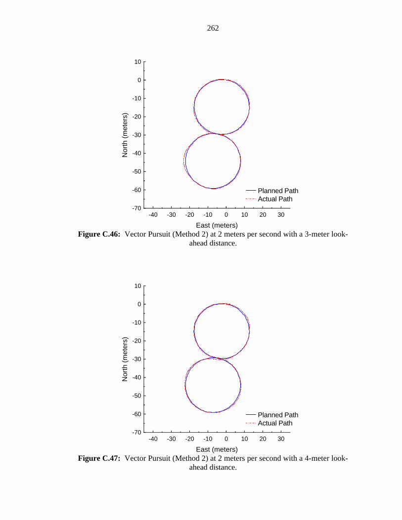
262
-40 -30 -20 -10 0 10 20 30-70
-60
-50
-40
-30
-20
-10
0
10
East (meters)
Nor
th (
met
ers)
Planned PathActual Path
Figure C.46: Vector Pursuit (Method 2) at 2 meters per second with a 3-meter look-
ahead distance.
-40 -30 -20 -10 0 10 20 30-70
-60
-50
-40
-30
-20
-10
0
10
East (meters)
Nor
th (
met
ers)
Planned PathActual Path
Figure C.47: Vector Pursuit (Method 2) at 2 meters per second with a 4-meter look-
ahead distance.
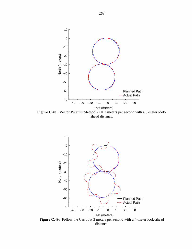
263
-40 -30 -20 -10 0 10 20 30-70
-60
-50
-40
-30
-20
-10
0
10
East (meters)
Nor
th (
met
ers)
Planned PathActual Path
Figure C.48: Vector Pursuit (Method 2) at 2 meters per second with a 5-meter look-
ahead distance.
-40 -30 -20 -10 0 10 20 30-70
-60
-50
-40
-30
-20
-10
0
10
East (meters)
Nor
th (
met
ers)
Planned PathActual Path
Figure C.49: Follow the Carrot at 3 meters per second with a 4-meter look-ahead
distance.
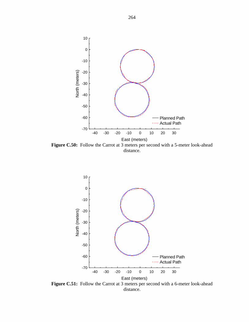
264
-40 -30 -20 -10 0 10 20 30-70
-60
-50
-40
-30
-20
-10
0
10
East (meters)
Nor
th (
met
ers)
Planned PathActual Path
Figure C.50: Follow the Carrot at 3 meters per second with a 5-meter look-ahead
distance.
-40 -30 -20 -10 0 10 20 30-70
-60
-50
-40
-30
-20
-10
0
10
East (meters)
Nor
th (
met
ers)
Planned PathActual Path
Figure C.51: Follow the Carrot at 3 meters per second with a 6-meter look-ahead
distance.
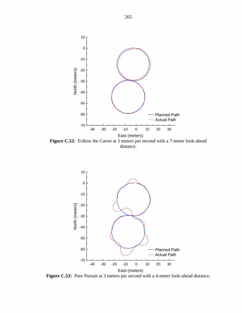
265
-40 -30 -20 -10 0 10 20 30-70
-60
-50
-40
-30
-20
-10
0
10
East (meters)
Nor
th (
met
ers)
Planned PathActual Path
Figure C.52: Follow the Carrot at 3 meters per second with a 7-meter look-ahead
distance.
-40 -30 -20 -10 0 10 20 30-70
-60
-50
-40
-30
-20
-10
0
10
East (meters)
Nor
th (
met
ers)
Planned PathActual Path
Figure C.53: Pure Pursuit at 3 meters per second with a 4-meter look-ahead distance.
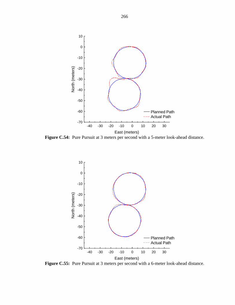
266
-40 -30 -20 -10 0 10 20 30-70
-60
-50
-40
-30
-20
-10
0
10
East (meters)
Nor
th (
met
ers)
Planned PathActual Path
Figure C.54: Pure Pursuit at 3 meters per second with a 5-meter look-ahead distance.
-40 -30 -20 -10 0 10 20 30-70
-60
-50
-40
-30
-20
-10
0
10
East (meters)
Nor
th (
met
ers)
Planned PathActual Path
Figure C.55: Pure Pursuit at 3 meters per second with a 6-meter look-ahead distance.

267
-40 -30 -20 -10 0 10 20 30-70
-60
-50
-40
-30
-20
-10
0
10
East (meters)
Nor
th (
met
ers)
Planned PathActual Path
Figure C.56: Pure Pursuit at 3 meters per second with a 7-meter look-ahead distance.
-40 -30 -20 -10 0 10 20 30-70
-60
-50
-40
-30
-20
-10
0
10
East (meters)
Nor
th (
met
ers)
Planned PathActual Path
Figure C.57: Vector Pursuit (Method 2) at 3 meters per second with a 4-meter look-
ahead distance.

268
-40 -30 -20 -10 0 10 20 30-70
-60
-50
-40
-30
-20
-10
0
10
East (meters)
Nor
th (
met
ers)
Planned PathActual Path
Figure C.58: Vector Pursuit (Method 2) at 3 meters per second with a 5-meter look-
ahead distance.
-40 -30 -20 -10 0 10 20 30-70
-60
-50
-40
-30
-20
-10
0
10
East (meters)
Nor
th (
met
ers)
Planned PathActual Path
Figure C.59: Vector Pursuit (Method 2) at 3 meters per second with a 6-meter look-
ahead distance.
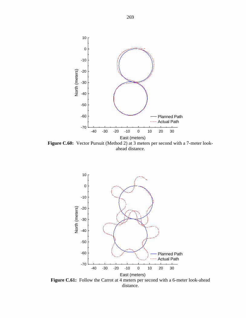
269
-40 -30 -20 -10 0 10 20 30-70
-60
-50
-40
-30
-20
-10
0
10
East (meters)
Nor
th (
met
ers)
Planned PathActual Path
Figure C.60: Vector Pursuit (Method 2) at 3 meters per second with a 7-meter look-
ahead distance.
-40 -30 -20 -10 0 10 20 30-70
-60
-50
-40
-30
-20
-10
0
10
East (meters)
Nor
th (
met
ers)
Planned PathActual Path
Figure C.61: Follow the Carrot at 4 meters per second with a 6-meter look-ahead
distance.
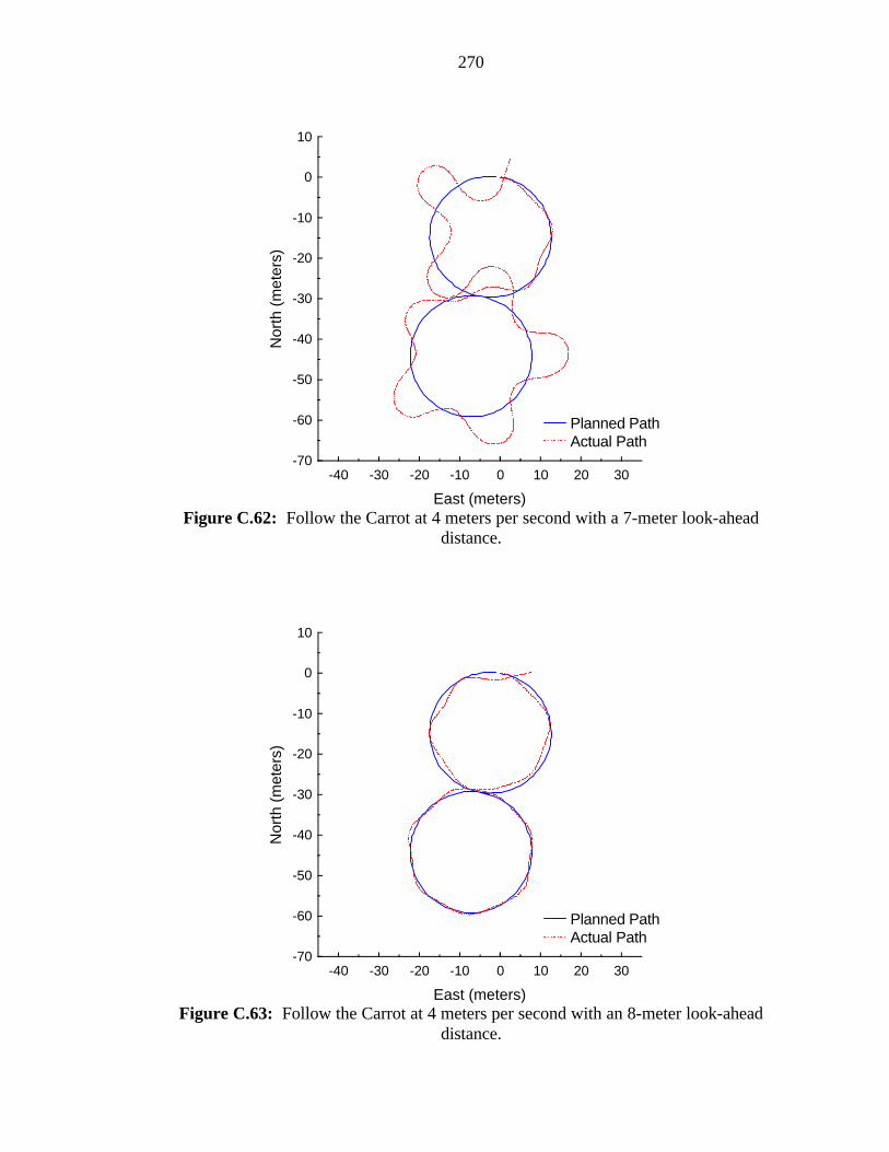
270
-40 -30 -20 -10 0 10 20 30-70
-60
-50
-40
-30
-20
-10
0
10
East (meters)
Nor
th (
met
ers)
Planned PathActual Path
Figure C.62: Follow the Carrot at 4 meters per second with a 7-meter look-ahead
distance.
-40 -30 -20 -10 0 10 20 30-70
-60
-50
-40
-30
-20
-10
0
10
East (meters)
Nor
th (
met
ers)
Planned PathActual Path
Figure C.63: Follow the Carrot at 4 meters per second with an 8-meter look-ahead
distance.

271
-40 -30 -20 -10 0 10 20 30-70
-60
-50
-40
-30
-20
-10
0
10
East (meters)
Nor
th (
met
ers)
Planned PathActual Path
Figure C.64: Follow the Carrot at 4 meters per second with a 9-meter look-ahead
distance.
-40 -30 -20 -10 0 10 20 30-70
-60
-50
-40
-30
-20
-10
0
10
East (meters)
Nor
th (
met
ers)
Planned PathActual Path
Figure C.65: Pure Pursuit at 4 meters per second with a 6-meter look-ahead distance.
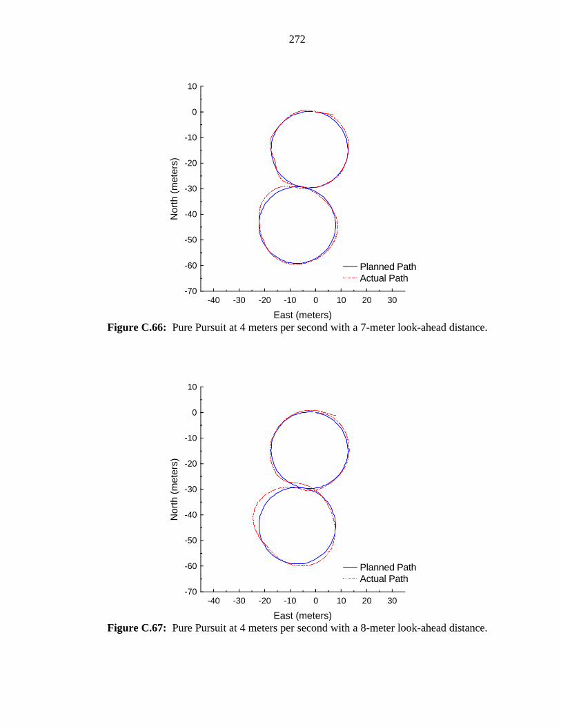
272
-40 -30 -20 -10 0 10 20 30-70
-60
-50
-40
-30
-20
-10
0
10
East (meters)
Nor
th (
met
ers)
Planned PathActual Path
Figure C.66: Pure Pursuit at 4 meters per second with a 7-meter look-ahead distance.
-40 -30 -20 -10 0 10 20 30-70
-60
-50
-40
-30
-20
-10
0
10
East (meters)
Nor
th (
met
ers)
Planned PathActual Path
Figure C.67: Pure Pursuit at 4 meters per second with a 8-meter look-ahead distance.
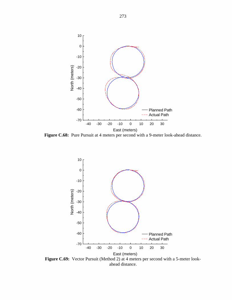
273
-40 -30 -20 -10 0 10 20 30-70
-60
-50
-40
-30
-20
-10
0
10
East (meters)
Nor
th (
met
ers)
Planned PathActual Path
Figure C.68: Pure Pursuit at 4 meters per second with a 9-meter look-ahead distance.
-40 -30 -20 -10 0 10 20 30-70
-60
-50
-40
-30
-20
-10
0
10
East (meters)
Nor
th (
met
ers)
Planned PathActual Path
Figure C.69: Vector Pursuit (Method 2) at 4 meters per second with a 5-meter look-
ahead distance.
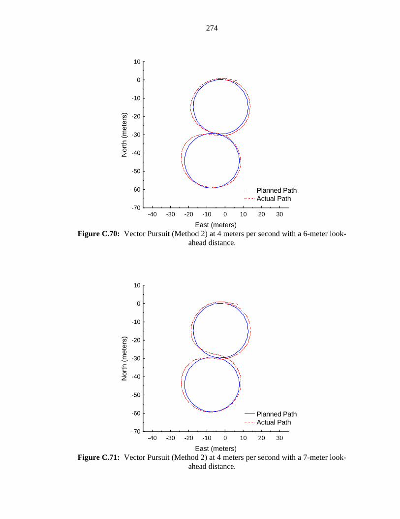
274
-40 -30 -20 -10 0 10 20 30-70
-60
-50
-40
-30
-20
-10
0
10
East (meters)
Nor
th (
met
ers)
Planned PathActual Path
Figure C.70: Vector Pursuit (Method 2) at 4 meters per second with a 6-meter look-
ahead distance.
-40 -30 -20 -10 0 10 20 30-70
-60
-50
-40
-30
-20
-10
0
10
East (meters)
Nor
th (
met
ers)
Planned PathActual Path
Figure C.71: Vector Pursuit (Method 2) at 4 meters per second with a 7-meter look-
ahead distance.
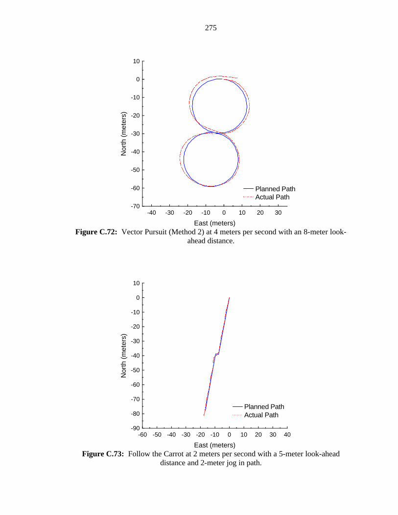
275
-40 -30 -20 -10 0 10 20 30-70
-60
-50
-40
-30
-20
-10
0
10
East (meters)
Nor
th (
met
ers)
Planned PathActual Path
Figure C.72: Vector Pursuit (Method 2) at 4 meters per second with an 8-meter look-
ahead distance.
-60 -50 -40 -30 -20 -10 0 10 20 30 40-90
-80
-70
-60
-50
-40
-30
-20
-10
0
10
East (meters)
Nor
th (
met
ers)
Planned PathActual Path
Figure C.73: Follow the Carrot at 2 meters per second with a 5-meter look-ahead
distance and 2-meter jog in path.
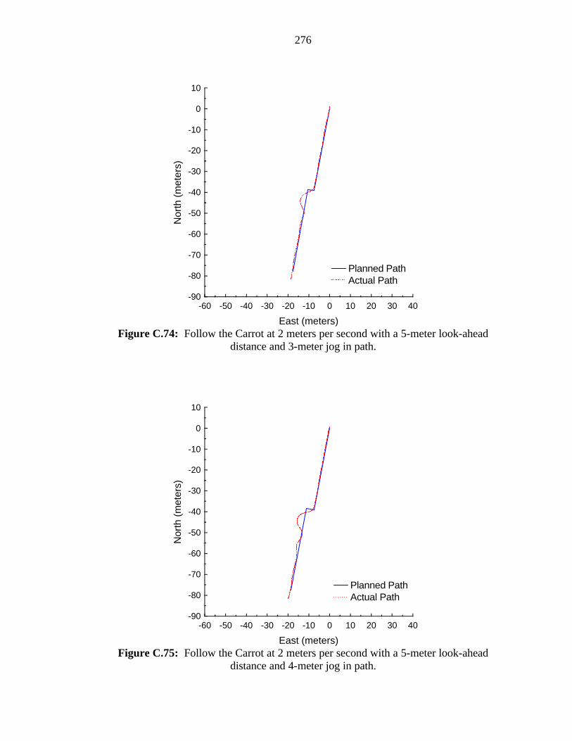
276
-60 -50 -40 -30 -20 -10 0 10 20 30 40-90
-80
-70
-60
-50
-40
-30
-20
-10
0
10
East (meters)
Nor
th (
met
ers)
Planned PathActual Path
Figure C.74: Follow the Carrot at 2 meters per second with a 5-meter look-ahead
distance and 3-meter jog in path.
-60 -50 -40 -30 -20 -10 0 10 20 30 40-90
-80
-70
-60
-50
-40
-30
-20
-10
0
10
East (meters)
Nor
th (
met
ers)
Planned PathActual Path
Figure C.75: Follow the Carrot at 2 meters per second with a 5-meter look-ahead
distance and 4-meter jog in path.
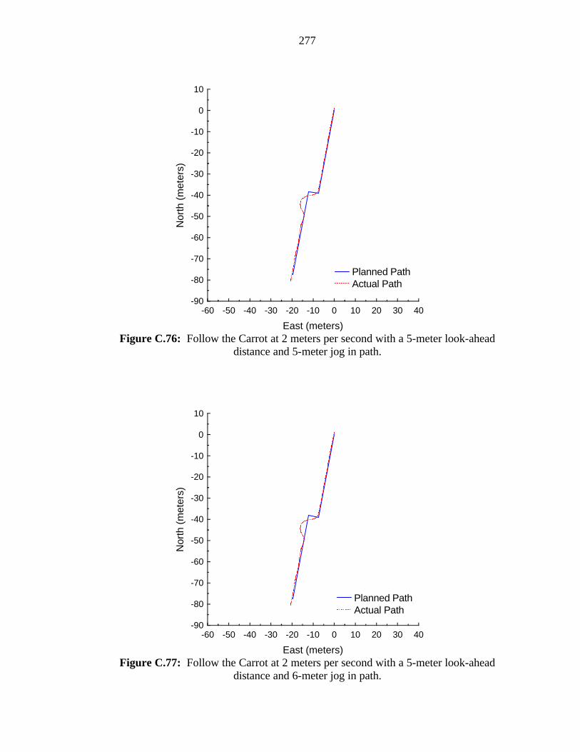
277
-60 -50 -40 -30 -20 -10 0 10 20 30 40-90
-80
-70
-60
-50
-40
-30
-20
-10
0
10
East (meters)
Nor
th (
met
ers)
Planned PathActual Path
Figure C.76: Follow the Carrot at 2 meters per second with a 5-meter look-ahead
distance and 5-meter jog in path.
-60 -50 -40 -30 -20 -10 0 10 20 30 40-90
-80
-70
-60
-50
-40
-30
-20
-10
0
10
East (meters)
Nor
th (
met
ers)
Planned PathActual Path
Figure C.77: Follow the Carrot at 2 meters per second with a 5-meter look-ahead
distance and 6-meter jog in path.

278
-60 -50 -40 -30 -20 -10 0 10 20 30 40-90
-80
-70
-60
-50
-40
-30
-20
-10
0
10
East (meters)
Nor
th (
met
ers)
Planned PathActual Path
Figure C.78: Pure Pursuit at 2 meters per second with a 5-meter look-ahead distance and
2-meter jog in path.
-60 -50 -40 -30 -20 -10 0 10 20 30 40-90
-80
-70
-60
-50
-40
-30
-20
-10
0
10
East (meters)
Nor
th (
met
ers)
Planned PathActual Path
Figure C.79: Pure Pursuit at 2 meters per second with a 5-meter look-ahead distance and
3-meter jog in path.
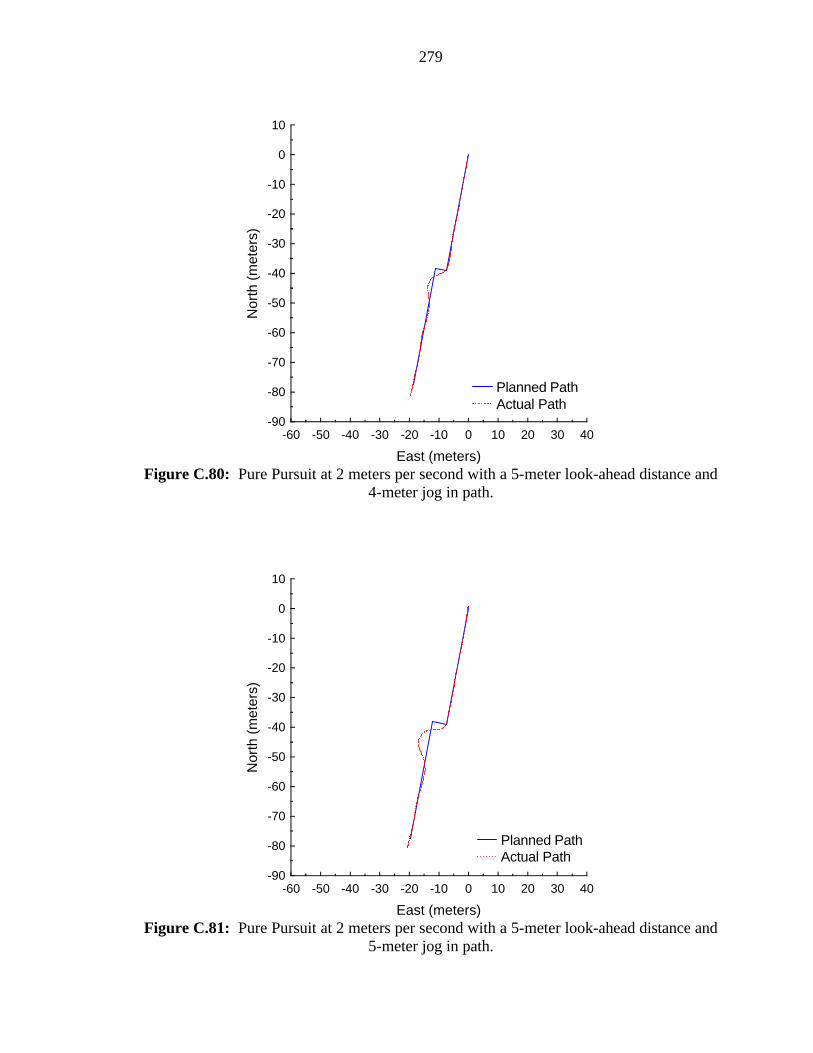
279
-60 -50 -40 -30 -20 -10 0 10 20 30 40-90
-80
-70
-60
-50
-40
-30
-20
-10
0
10
East (meters)
Nor
th (
met
ers)
Planned PathActual Path
Figure C.80: Pure Pursuit at 2 meters per second with a 5-meter look-ahead distance and
4-meter jog in path.
-60 -50 -40 -30 -20 -10 0 10 20 30 40-90
-80
-70
-60
-50
-40
-30
-20
-10
0
10
East (meters)
Nor
th (
met
ers)
Planned PathActual Path
Figure C.81: Pure Pursuit at 2 meters per second with a 5-meter look-ahead distance and
5-meter jog in path.

280
-60 -50 -40 -30 -20 -10 0 10 20 30 40-90
-80
-70
-60
-50
-40
-30
-20
-10
0
10
East (meters)
Nor
th (
met
ers)
Planned PathActual Path
Figure C.82: Pure Pursuit at 2 meters per second with a 5-meter look-ahead distance and
6-meter jog in path.
-60 -50 -40 -30 -20 -10 0 10 20 30 40-90
-80
-70
-60
-50
-40
-30
-20
-10
0
10
East (meters)
Nor
th (
met
ers)
Planned PathActual Path
Figure C.83: Vector Pursuit (Method 2) at 2 meters per second with a 5-meter look-
ahead distance and 2-meter jog in path.
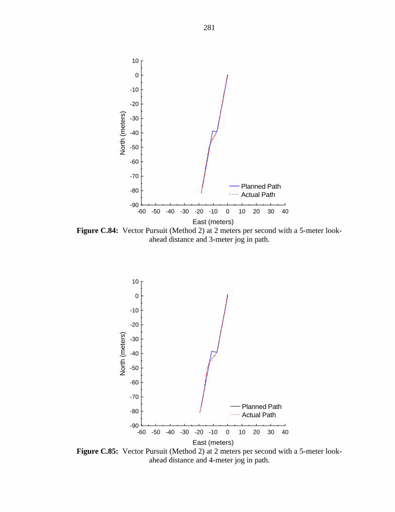
281
-60 -50 -40 -30 -20 -10 0 10 20 30 40-90
-80
-70
-60
-50
-40
-30
-20
-10
0
10
East (meters)
Nor
th (
met
ers)
Planned PathActual Path
Figure C.84: Vector Pursuit (Method 2) at 2 meters per second with a 5-meter look-
ahead distance and 3-meter jog in path.
-60 -50 -40 -30 -20 -10 0 10 20 30 40-90
-80
-70
-60
-50
-40
-30
-20
-10
0
10
East (meters)
Nor
th (
met
ers)
Planned PathActual Path
Figure C.85: Vector Pursuit (Method 2) at 2 meters per second with a 5-meter look-
ahead distance and 4-meter jog in path.
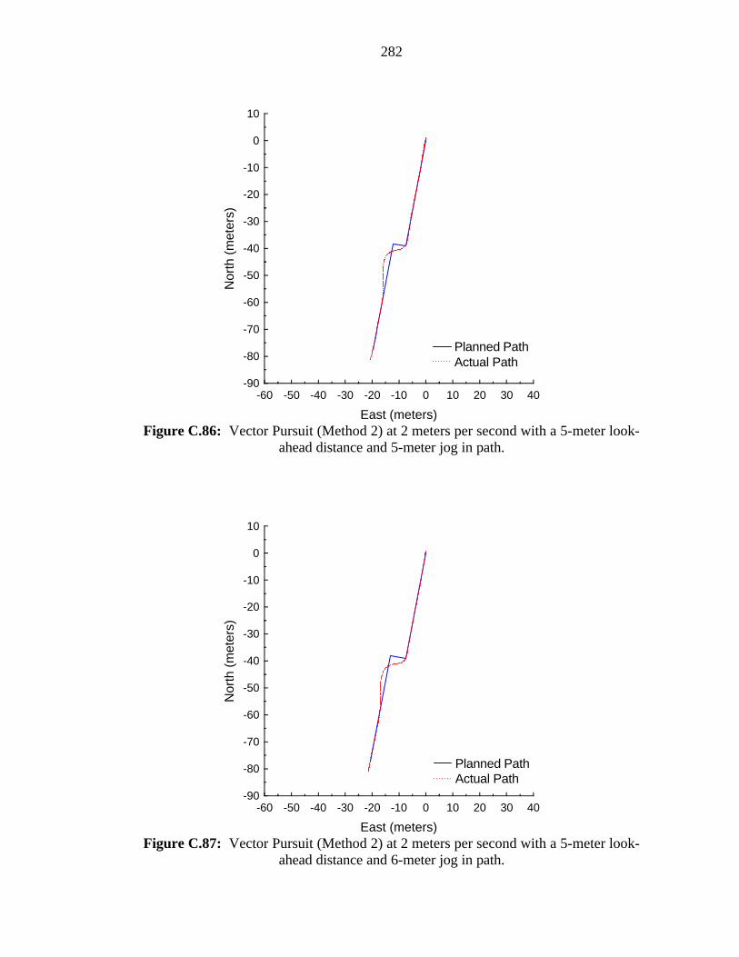
282
-60 -50 -40 -30 -20 -10 0 10 20 30 40-90
-80
-70
-60
-50
-40
-30
-20
-10
0
10
East (meters)
Nor
th (
met
ers)
Planned PathActual Path
Figure C.86: Vector Pursuit (Method 2) at 2 meters per second with a 5-meter look-
ahead distance and 5-meter jog in path.
-60 -50 -40 -30 -20 -10 0 10 20 30 40-90
-80
-70
-60
-50
-40
-30
-20
-10
0
10
East (meters)
Nor
th (
met
ers)
Planned PathActual Path
Figure C.87: Vector Pursuit (Method 2) at 2 meters per second with a 5-meter look-
ahead distance and 6-meter jog in path.

283
-60 -50 -40 -30 -20 -10 0 10 20 30 40-90
-80
-70
-60
-50
-40
-30
-20
-10
0
10
East (meters)
Nor
th (
met
ers)
Planned PathActual Path
Figure C.88: Follow the Carrot at 3 meters per second with a 7-meter look-ahead
distance and 2-meter jog in path.
-60 -50 -40 -30 -20 -10 0 10 20 30 40-90
-80
-70
-60
-50
-40
-30
-20
-10
0
10
East (meters)
Nor
th (
met
ers)
Planned PathActual Path
Figure C.89: Follow the Carrot at 3 meters per second with a 7-meter look-ahead
distance and 3-meter jog in path.
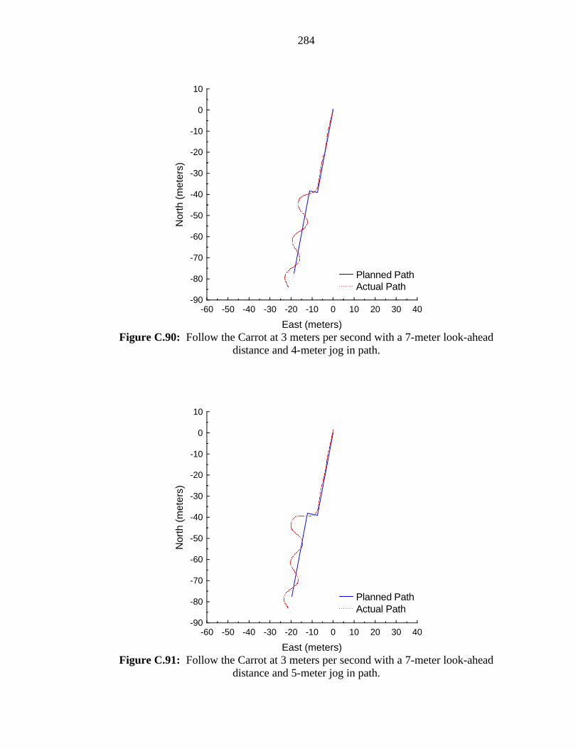
284
-60 -50 -40 -30 -20 -10 0 10 20 30 40-90
-80
-70
-60
-50
-40
-30
-20
-10
0
10
East (meters)
Nor
th (
met
ers)
Planned PathActual Path
Figure C.90: Follow the Carrot at 3 meters per second with a 7-meter look-ahead
distance and 4-meter jog in path.
-60 -50 -40 -30 -20 -10 0 10 20 30 40-90
-80
-70
-60
-50
-40
-30
-20
-10
0
10
East (meters)
Nor
th (
met
ers)
Planned PathActual Path
Figure C.91: Follow the Carrot at 3 meters per second with a 7-meter look-ahead
distance and 5-meter jog in path.

285
-60 -50 -40 -30 -20 -10 0 10 20 30 40-90
-80
-70
-60
-50
-40
-30
-20
-10
0
10
East (meters)
Nor
th (
met
ers)
Planned PathActual Path
Figure C.92: Follow the Carrot at 3 meters per second with a 7-meter look-ahead
distance and 6-meter jog in path.
-60 -50 -40 -30 -20 -10 0 10 20 30 40-90
-80
-70
-60
-50
-40
-30
-20
-10
0
10
East (meters)
Nor
th (
met
ers)
Planned PathActual Path
Figure C.93: Pure Pursuit at 3 meters per second with a 7-meter look-ahead distance and
2-meter jog in path.

286
-60 -50 -40 -30 -20 -10 0 10 20 30 40-90
-80
-70
-60
-50
-40
-30
-20
-10
0
10
East (meters)
Nor
th (
met
ers)
Planned PathActual Path
Figure C.94: Pure Pursuit at 3 meters per second with a 7-meter look-ahead distance and
3-meter jog in path.
-60 -50 -40 -30 -20 -10 0 10 20 30 40-90
-80
-70
-60
-50
-40
-30
-20
-10
0
10
East (meters)
Nor
th (
met
ers)
Planned PathActual Path
Figure C.95: Pure Pursuit at 3 meters per second with a 7-meter look-ahead distance and
4-meter jog in path.
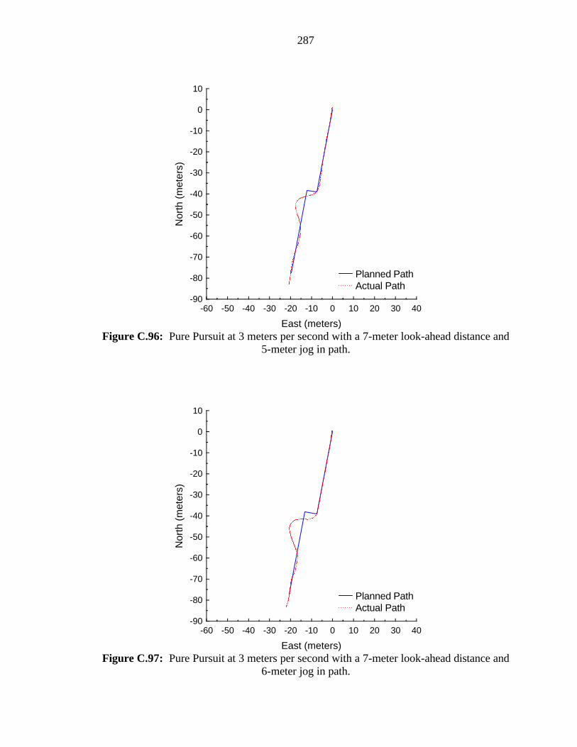
287
-60 -50 -40 -30 -20 -10 0 10 20 30 40-90
-80
-70
-60
-50
-40
-30
-20
-10
0
10
East (meters)
Nor
th (
met
ers)
Planned PathActual Path
Figure C.96: Pure Pursuit at 3 meters per second with a 7-meter look-ahead distance and
5-meter jog in path.
-60 -50 -40 -30 -20 -10 0 10 20 30 40-90
-80
-70
-60
-50
-40
-30
-20
-10
0
10
East (meters)
Nor
th (
met
ers)
Planned PathActual Path
Figure C.97: Pure Pursuit at 3 meters per second with a 7-meter look-ahead distance and
6-meter jog in path.
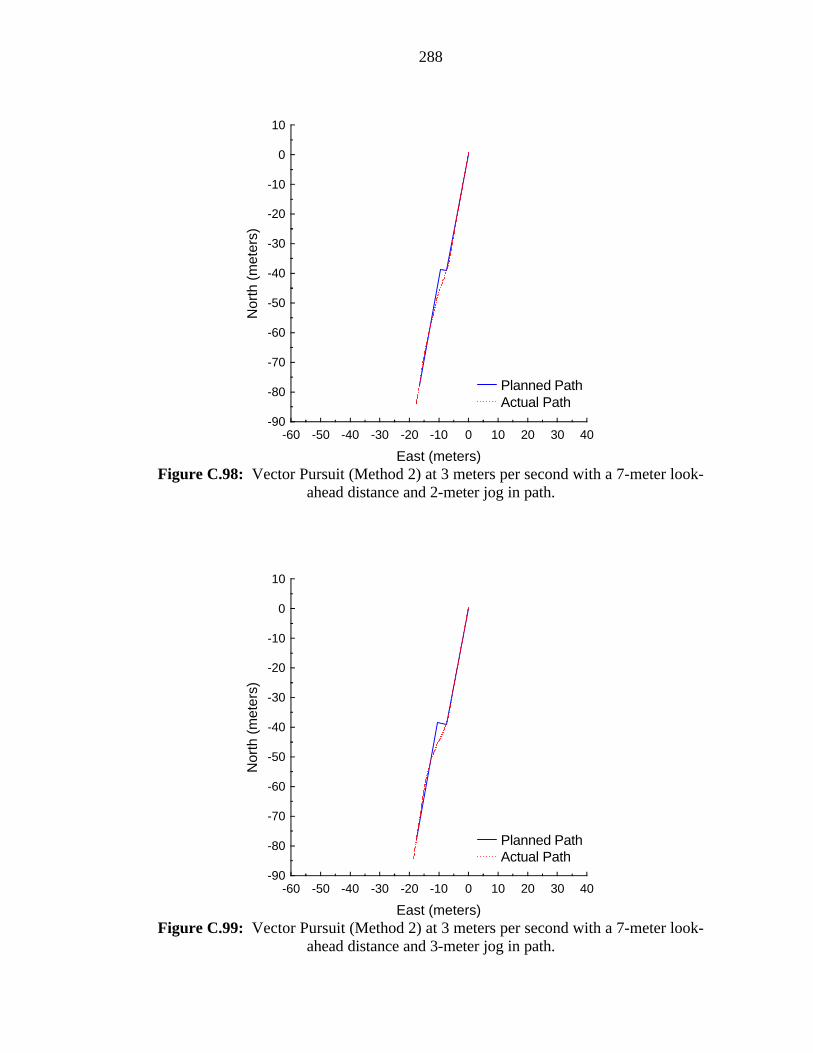
288
-60 -50 -40 -30 -20 -10 0 10 20 30 40-90
-80
-70
-60
-50
-40
-30
-20
-10
0
10
East (meters)
Nor
th (
met
ers)
Planned PathActual Path
Figure C.98: Vector Pursuit (Method 2) at 3 meters per second with a 7-meter look-
ahead distance and 2-meter jog in path.
-60 -50 -40 -30 -20 -10 0 10 20 30 40-90
-80
-70
-60
-50
-40
-30
-20
-10
0
10
East (meters)
Nor
th (
met
ers)
Planned PathActual Path
Figure C.99: Vector Pursuit (Method 2) at 3 meters per second with a 7-meter look-
ahead distance and 3-meter jog in path.
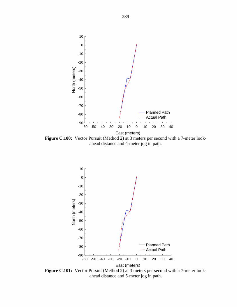
289
-60 -50 -40 -30 -20 -10 0 10 20 30 40-90
-80
-70
-60
-50
-40
-30
-20
-10
0
10
East (meters)
Nor
th (
met
ers)
Planned PathActual Path
Figure C.100: Vector Pursuit (Method 2) at 3 meters per second with a 7-meter look-
ahead distance and 4-meter jog in path.
-60 -50 -40 -30 -20 -10 0 10 20 30 40-90
-80
-70
-60
-50
-40
-30
-20
-10
0
10
East (meters)
Nor
th (
met
ers)
Planned PathActual Path
Figure C.101: Vector Pursuit (Method 2) at 3 meters per second with a 7-meter look-
ahead distance and 5-meter jog in path.
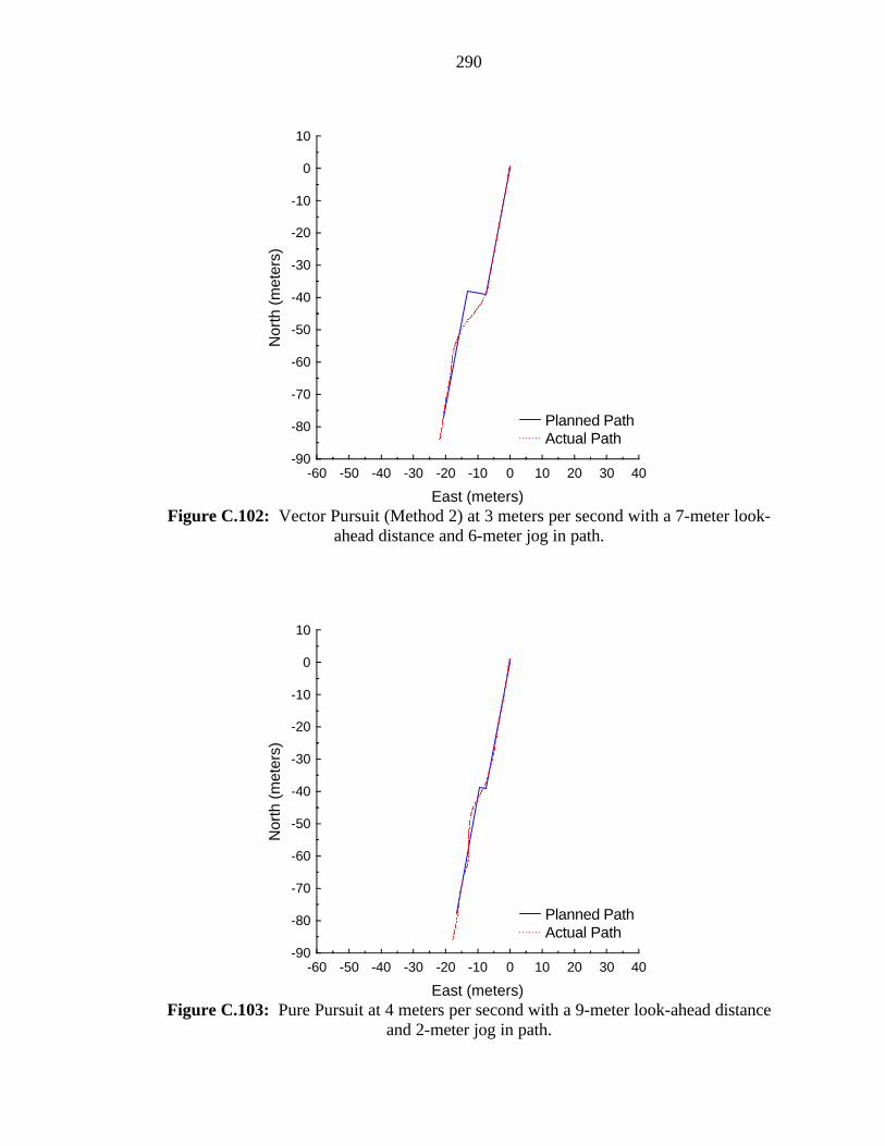
290
-60 -50 -40 -30 -20 -10 0 10 20 30 40-90
-80
-70
-60
-50
-40
-30
-20
-10
0
10
East (meters)
Nor
th (
met
ers)
Planned PathActual Path
Figure C.102: Vector Pursuit (Method 2) at 3 meters per second with a 7-meter look-
ahead distance and 6-meter jog in path.
-60 -50 -40 -30 -20 -10 0 10 20 30 40-90
-80
-70
-60
-50
-40
-30
-20
-10
0
10
East (meters)
Nor
th (
met
ers)
Planned PathActual Path
Figure C.103: Pure Pursuit at 4 meters per second with a 9-meter look-ahead distance
and 2-meter jog in path.

291
-60 -50 -40 -30 -20 -10 0 10 20 30 40-90
-80
-70
-60
-50
-40
-30
-20
-10
0
10
East (meters)
Nor
th (
met
ers)
Planned PathActual Path
Figure C.104: Pure Pursuit at 4 meters per second with a 9-meter look-ahead distance
and 3-meter jog in path.
-60 -50 -40 -30 -20 -10 0 10 20 30 40-90
-80
-70
-60
-50
-40
-30
-20
-10
0
10
East (meters)
Nor
th (
met
ers)
Planned PathActual Path
Figure C.105: Pure Pursuit at 4 meters per second with a 9-meter look-ahead distance
and 4-meter jog in path.
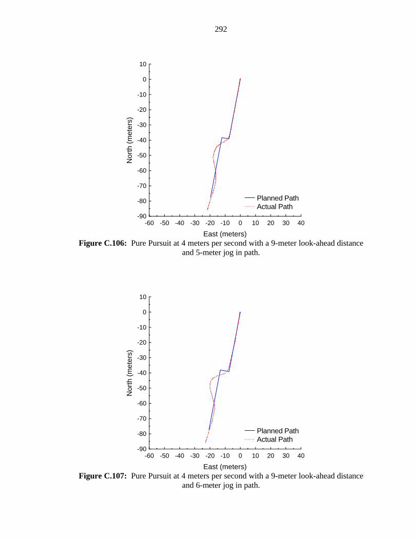
292
-60 -50 -40 -30 -20 -10 0 10 20 30 40-90
-80
-70
-60
-50
-40
-30
-20
-10
0
10
East (meters)
Nor
th (
met
ers)
Planned PathActual Path
Figure C.106: Pure Pursuit at 4 meters per second with a 9-meter look-ahead distance
and 5-meter jog in path.
-60 -50 -40 -30 -20 -10 0 10 20 30 40-90
-80
-70
-60
-50
-40
-30
-20
-10
0
10
East (meters)
Nor
th (
met
ers)
Planned PathActual Path
Figure C.107: Pure Pursuit at 4 meters per second with a 9-meter look-ahead distance
and 6-meter jog in path.

293
-60 -50 -40 -30 -20 -10 0 10 20 30 40-90
-80
-70
-60
-50
-40
-30
-20
-10
0
10
East (meters)
Nor
th (
met
ers)
Planned PathActual Path
Figure C.108: Vector Pursuit (Method 2) at 4 meters per second with a 9-meter look-
ahead distance and 2-meter jog in path.
-60 -50 -40 -30 -20 -10 0 10 20 30 40-90
-80
-70
-60
-50
-40
-30
-20
-10
0
10
East (meters)
Nor
th (
met
ers)
Planned PathActual Path
Figure C.109: Vector Pursuit (Method 2) at 4 meters per second with a 9-meter look-
ahead distance and 3-meter jog in path.
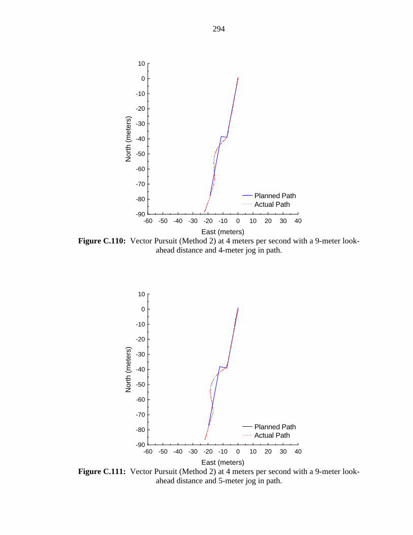
294
-60 -50 -40 -30 -20 -10 0 10 20 30 40-90
-80
-70
-60
-50
-40
-30
-20
-10
0
10
East (meters)
Nor
th (
met
ers)
Planned PathActual Path
Figure C.110: Vector Pursuit (Method 2) at 4 meters per second with a 9-meter look-
ahead distance and 4-meter jog in path.
-60 -50 -40 -30 -20 -10 0 10 20 30 40-90
-80
-70
-60
-50
-40
-30
-20
-10
0
10
East (meters)
Nor
th (
met
ers)
Planned PathActual Path
Figure C.111: Vector Pursuit (Method 2) at 4 meters per second with a 9-meter look-
ahead distance and 5-meter jog in path.

295
-60 -50 -40 -30 -20 -10 0 10 20 30 40-90
-80
-70
-60
-50
-40
-30
-20
-10
0
10
East (meters)
Nor
th (
met
ers)
Planned PathActual Path
Figure C.112: Vector Pursuit (Method 2) at 4 meters per second with a 9-meter look-
ahead distance and 6-meter jog in path.
-80 -60 -40 -20 0 20-80
-70
-60
-50
-40
-30
-20
-10
0
10
East (meters)
Nor
th (
met
ers)
Planned PathActual Path
Figure C.113: Vector Pursuit (Method 2) at -2 meters per second with a 4-meter look-
ahead distance.
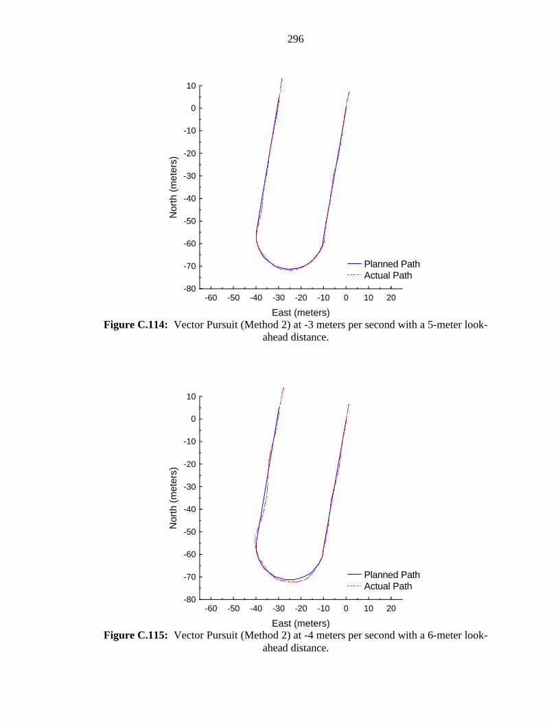
296
-60 -50 -40 -30 -20 -10 0 10 20-80
-70
-60
-50
-40
-30
-20
-10
0
10
East (meters)
Nor
th (
met
ers)
Planned PathActual Path
Figure C.114: Vector Pursuit (Method 2) at -3 meters per second with a 5-meter look-
ahead distance.
-60 -50 -40 -30 -20 -10 0 10 20-80
-70
-60
-50
-40
-30
-20
-10
0
10
East (meters)
Nor
th (
met
ers)
Planned PathActual Path
Figure C.115: Vector Pursuit (Method 2) at -4 meters per second with a 6-meter look-
ahead distance.
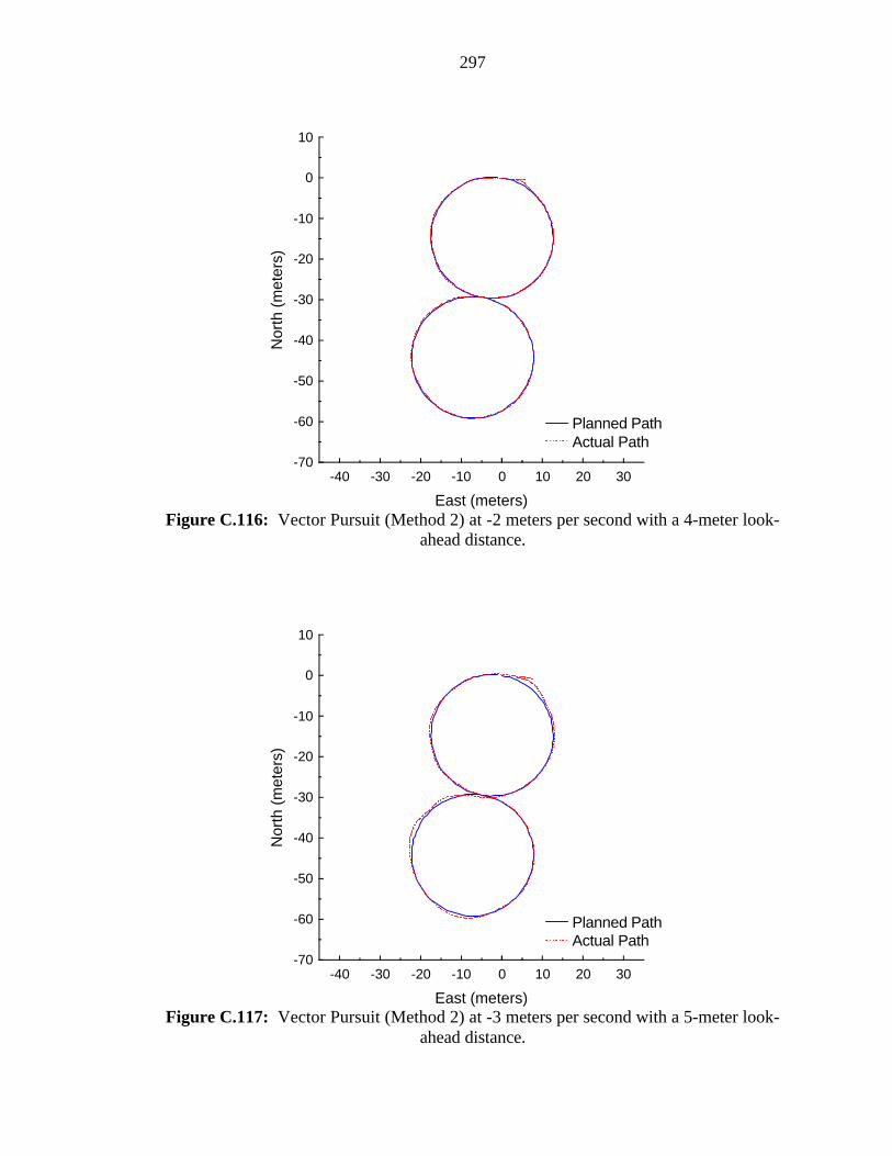
297
-40 -30 -20 -10 0 10 20 30-70
-60
-50
-40
-30
-20
-10
0
10
East (meters)
Nor
th (
met
ers)
Planned PathActual Path
Figure C.116: Vector Pursuit (Method 2) at -2 meters per second with a 4-meter look-
ahead distance.
-40 -30 -20 -10 0 10 20 30-70
-60
-50
-40
-30
-20
-10
0
10
East (meters)
Nor
th (
met
ers)
Planned PathActual Path
Figure C.117: Vector Pursuit (Method 2) at -3 meters per second with a 5-meter look-
ahead distance.
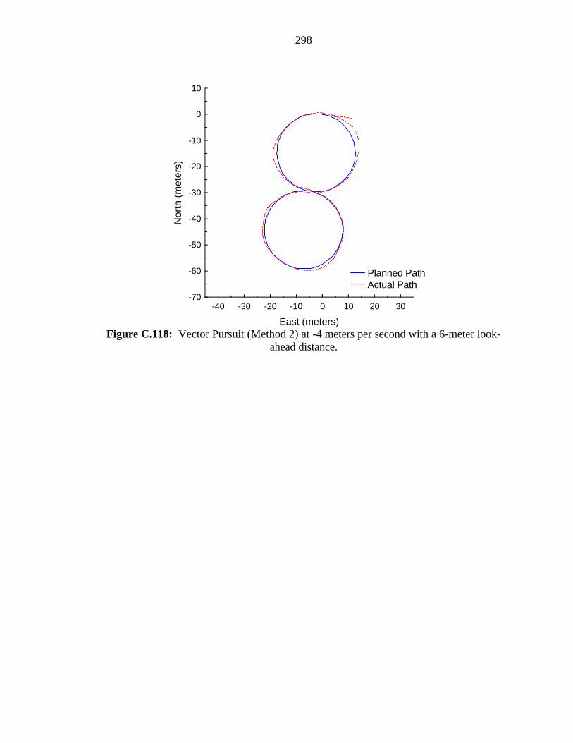
298
-40 -30 -20 -10 0 10 20 30-70
-60
-50
-40
-30
-20
-10
0
10
East (meters)
Nor
th (
met
ers)
Planned PathActual Path
Figure C.118: Vector Pursuit (Method 2) at -4 meters per second with a 6-meter look-
ahead distance.

299
LIST OF REFERENCES
[1] Goldberg, K., et al., Algorithmic Foundations of Robotics / WAFR 94, the Workshop on the Algorithmic Foundation of Robotics, A.K. Peters, Wellesley, Massachusetts, 1995.
[2] Green, D.N., Sasiadek, J.Z. and Vukovich, G.S., “Guidance and Control of an
Autonomous Planetary Rover,” Proceedings of the IEEE-IEE Vehicle Navigation and Informations Systems Conference, Ottawa, Ontario, Canada, 1993, p539-542.
[3] Green, D.N., Sasiadek, J.Z. and Vukovich, G.S., “Path Tracking, Obstacle Avoidance
and Position Estimation by an Autonomous Wheeled Planetary Rover,” Proceedings of the 1994 IEEE International Conference on Robotics and Automation, San Diego, CA, 1994, p1300-1305.
[4] Boissier, L., “IARES-L: A Ground Demonstrator of Planetary Rover Technologies,”
Robotics and Autonomous Systems, v23, 1998, p89-97. [5] O’Connor, M., Bell, T., Elkaim, G. and Parkinson, B., “Automatic Steering of Farm
Vehicles Using GPS,” Stanford University, California. [6] Marchant, J. A., Hague, T. and Tillet, N. D., “Row-following accuracy of an
autonomous vision-guided agricultural vehicle,” Computers and Electronics in Agriculture, v16, n2, January 1997, p165-175.
[7] Hofner, C. and Schmidt, G., “Path Planning and Guidance Techniques for an
Autonomous Mobile Cleaning Robot,” Robotic and Autonomous Systems, v14, n2-3, May 1995, p199-212.
[8] Schmidt, G. and Hofner, C., “Advanced Planning and Navigation Approach for
Autonomous Cleaning Robot Operations,” Proceedings of the 1998 IEEE/RSJ International Conference on Intelligent Robots and Systems, Victoria, Canada, 1998, p1230-1235.
[9] Ulrich, I., Mondada, F. and Nicoud, J.-D., “Autonomous vacuum cleaner,” Robotics
and Autonomous Systems, v19, n3-4, March 1997, p233-245. [10] Nolfi, S., “Evolving non-trivial behaviors on real robots: A garbage collecting
robot,” Robotics and Autonomous Systems, v22, n3-4, December 1997, p187-198.

300
[11] Spooner, J. T. and Passino, K. M., “Stable Adaptive Fuzzy Control for an Automated Highway System,” IEEE International Conference on Intelligent Control, Monterey, CA, 1995, p531-536.
[12] Huang, S. and Ren, W., “Vehicle longitudinal control using throttles and brakes,”
Robotics and Autonomous Systems, v26, n4, March 1999, p241-253. [13] Unyelioglu, K. A., Hatipoglu, C. and Ozguner, U., “Design and Stability Analysis of
a Lane Following Controller,” IEEE Transactions on Control Systems Technology, v5, n1, January 1997, p127-134.
[14] O’Brien, R. T., Iglesias, P. A. and Urban, T. J., “Vehicle Lateral Control for
Automated Highway Systems,” IEEE Transactions on Control Systems Technology, v4, n3, 1996, p266-273.
[15] Hsu, J.-C., Chen, W.-L., Shien, K.H. and Yey, E.C., “Cooperative Copilot with
Active Steering Assistance for Vehicle Lane Keeping,” International Journal of Vehicle Design, v19, n1, 1998, p78-107.
[16] Gorinevsky, D., Kapitanovsky, A. and Goldenberg, A., “Neural Network
Architecture for Trajectory Generation and Control of Automated Car Parking,” IEEE Transactions on Control Systems Technology, v4, n1, January 1996, p50-56.
[17] Paromtchik, I.E. and Laugier, C., “Autonomous Parallel Parking of a Nonholonomic
Vehicle,” Proceedings of the 1996 IEEE Intelligent Vehicle Symposium, Tokyo, Japan, 1996, p13-18.
[18] Paromtchik, I.E. and Laugier, C., “Motion Generation and Control for Parking an
Autonomous Vehicle,” Proceedings of the 1996 IEEE 13th International Conference on Robotics and Automation, Minneapolis, MN, 1996, p3117-3122.
[19] Murphey, K. and Legowik, S., “GPS Aided Retrotraverse For Unmanned Ground
Vehicles,” SPIE 10th Annual AeroSense Symposium, Orlando, FL, April 1996. [20] Gage, D. W., "An Evolutionary Strategy for Achieving Autonomous Navigation,"
SPIE Proc. 3525: Mobile Robots XIII, Boston MA, November 1998. [21] Ciccimaro, D. A., Everett, H. R., Bruch, M. H., and Phillips, C. B., "A Supervised
Autonomous Security Response Robot," American Nuclear Society 8th International Topical Meeting on Robotics and Remote Systems (ANS'99), Pittsburgh, PA, April 1999.
[22] Pastore, T.H., Everett, H. R., and Bonner, K., "Mobile Robots for Outdoor Security
Applications," American Nuclear Society 8th International Topical Meeting on Robotics and Remote Systems (ANS'99), Pittsburgh, PA, April 1999.

301
[23] Koji, K., “Underwater Inspection Robot-AIRIS 21,” Nuclear Engineering and Design, v188, 1999, p367-371.
[24] Cordes, S., Berns, K., Eberl, M., Ilg, W. and Suna, R., “Autonomous sewer
inspection with a wheeled, multiarticulated robot,” Robotics and Autonomous Systems, v21, n1, July 1997, p123-135.
[25] Reif, J.H. and Wang, H., “Social Potential Fields: A Distributed Behavioral Control
for Autonomous Robots,” Robotics and Autonomous Systems, v27, 1999, p171-194.
[26] Barfoot, C. W. and Ibrahim, M. Y., “Development of an Adaptive Fuzzy
Behavioural Control System with Experimental and Industrial Applications,” Computers and Industrial Engineering, v34, n4, September 1998, p807-811.
[27] Castellano, G., Attolico, G. and Distante, A., “Automatic generation of fuzzy rules
for reactive robot controllers,” Robotics and Autonomous Systems, v22, n2, November 1997, p133-149.
[28] Lee, P.-S. and Wang, L.-L., “Collision Avoidance by Fuzzy Logic Control for
Automated Guided Vehicle Navigation,” Journal of Robotic Systems, v11, n8, 1994, p743-760.
[29] Martinez, A., Tunstel, E. and Jamshidi, M., “Fuzzy logic based collision avoidance
for a mobile robot,” Robotica, v12, 1994, p521-527. [30] Saffiotti, A., Ruspini, E. H. and Konolige, K., “Blending Reactivity and Goal-
Directedness in a Fuzzy Controller,” Proceedings of the Second IEEE Conference on Fuzzy Systems, San Francisco, CA, March 1993, pp. 134-139.
[31] Saffiotti, A., Ruspini, E. H. and Konolige, K., “Robust Execution of Robot Plans
Using Fuzzy Logic,” Fuzzy Logic in Artificial Intelligence - IJCAI `93 Workshop LNAI 847, Springer-Verlag, Berlin, DE, 1994, pp.24-37.
[32] Xu, W. L., Tso, S. K. and Fung, Y. H., “Fuzzy reactive control of a mobile robot
incorporating a real/virtual target switching strategy,” Robotics and Autonomous Systems, v23, n3, April 1998, p171-186.
[33] Floreano, D. and Mondada, F., “Evolutionary neurocontrollers for autonomous
mobile robots,” Neural Networks, v11, n7-8, October 1998, p1461-1478. [34] Reignier, P., Hansen, V. and Crowley, J. L., “Incremental supervised learning for
mobile robot reactive control,” Robotics and Autonomous Systems, v19, n3-4, March 1997, p247-257.
302
[35] Tani, J. and Fukumura, N. “Self-organizing Internal Representation in Learning of Naviagation: A Physical Experiment by the Mobile Robot YAMABICO,” Neural Networks, v10, n1, January 1997, p153-159.
[36] Ram, A., Arkin, R., Boone, G. and Pearce, M., “Using Genetic Algorithms to Learn
Reactive Control Parameters for Autonomous Robotic Navigation,” Adaptive Behavior, v2, n3, 1994, p277-304.
[37] Stafylopatis, A. and Blekas, K., “Autonomous vehicle navigation using evolutionary
reinforcement learning,” European Journal of Operational Research, v108, n2, July 1998, p306-318.
[38] Godjevac, J. and Steele, N., “Adaptive Fuzzy Controller for Robot Navigation,”
IEEE International Conference on Fuzzy Systems, v1, New Orleans, LA, 1996, p136-142.
[39] Li, W., Ma, C. and Wahl, F.M., “A neuro-fuzzy system architecture for behavior-
based control of a mobile robot in unknown environments,” Fuzzy Sets and Systems, v87, n2, April 1997, p133-140.
[40] Song, K.-T. and Sheen, L.-H., “Fuzzy-neuro Control Design for Obstacle Avoidance
of a Mobile Robot,” IEEE International Conference on Fuzzy Systems, v1, Yokohama, Japan, 1995, p71-76.
[41] Yung, N. H. C. and Ye, C., “An Adaptive Fuzzy Approach to Obstacle Avoidance,”
Proceedings of the IEEE International Conference on Systems, Man, and Cybernetics, v4, San Diego, CA, 1998, p3418-3423.
[42] Zhang, M., Peng, S. and Meng, Q., “Neural network and fuzzy logic techniques
based collision avoidance for a mobile robot,” Robotica, v15, 1997, p627-632. [43] Hoffman, F. and Pfister, G., “Evolutionary Design of a Fuzzy Knowledge Base for a
Mobile Robot,” International Journal of Approximate Reasoning, v17, n4, November 1997, p447-469.
[44] McFetridge, L. and Ibrahim, M. Y., “New Technique of Mobile Robot Navigation
Using a Hybrid Adaptive Fuzzy-potential Field Approach,” Computers & Industrial Engineering, v35, n3-4, December 1998, p471-474.
[45] Wu, K.-H., Chen, C.-H. and Ko, J.-M., “Path Planning and Prototype Design of an
AGV”, Mathematical and Computer Modelling, v30, 1999, p147-167. [46] Xiaowei, M. A., Xiaoli, L. I., Yulin, M. A. and Hegao, C. A. I., “Real-time Self-
reaction of Mobile Robot with Genetic Fuzzy Neural Network in Unknown Environment,” Proceedings of the IEEE International Conference on Systems, Man, and Cybernetics, v4, San Diego, CA, 1998, p3313-3318.
303
[47] Choi, S. B., The Design of a Look-Down Feedback Adaptive Controller for the Lateral Control of Front-Wheel-Steering Autonomous Highway Vehicles,” Proceedings of the American Control Conference, v3, Albuquerque, New Mexico, 1997, p1603-1607.
[48] DeSantis, R. M., “Modeling and path-tracking control of a mobile wheeled robot
with a differential drive,” Robotica, v13, 1995, p401-410. [49] Egerstedt, M. Hu, X. and Stotsky, A., “Control of a Car-Like Robot Using a
Dynamic Model,” IEEE International Conference on Robotics and Automation, v4, Leuven, Belgium, 1998, p3273-3278.
[50] Jagannathan, S., Zhu, S. Q. and Lewis, F. L., “Path planning and control of a mobile
base with nonholonomic constraints,” Robitica, v12, 1994, p529-539. [51] Kanayama, Y.J. and Fahroo, F., “A New Line Tracking Method for Nonholonomic
Vehicles,” Proceedings of the 1997 IEEE International Conference on Robotics and Automation, Albuquerque, NM, April 1997, p2908-2913.
[52] Lee, S. S. and Williams, J. H., “A fast tracking error control method for an
autonomous mobile robot,” Robotica, v11, 1993, p209-215. [53] Shin, D.H., Singh, S. and Lee, J.J., “Explicit Path Tracking By Autonomous
Vehicles,” Robotica, v10, 1992, p539-554. [54] Ku, C.-H. and Tsai, W.-H., “Smooth Vision-Based Autonomous Land Vehicle
Navigation in Indoor Environments by Person Following Using Sequential Pattern Recognition,” Journal of Robotic Systems, v16, n5, 1999, p249-262.
[55] Murphy, K.N., “Analysis of Robotic Vehicle Steering and Controller Delay,”
Proceedings of the Fifth International Symposium on Robotics and Manufacturing, Wailea, Maui, HI, August 1994.
[56] Ollero, A. and Heredia, G., "Stability analysis of mobile robot path tracking,"
Proceedings of the 1995 IEEE/RSJ International Conference on Intelligent Robots and Systems. Part 3 (of 3) Pittsburgh, PA, 1995. p 461-466.
[57] Balluchi, A., Bicchi, A., Balestrino, A. and Casalino, G., “Path Tracking Control for
Dubin’s Car,” Proceedings of the 1996 IEEE International Conference on Robotics and Automation, Minneapolis, MN, April 1996, p3123-3128.
[58] Yang, J.-M., Choi, I.-H. and Kim, J.-H., “Sliding Mode Control of a Nonholonomic
Wheeled Mobile Robot for Trajectory Tracking,” Proceedings of the 1998 IEEE International Conference on Robotics and Automation, Leuven, Belgium, May 1998, p2983-2988.
304
[59] Aguilar M., L. E., Soueres, P., Courdesses, M. and Fleury, S., “Robust Path-following Control with Exponential Stability for Mobile Robots,” IEEE International Conference on Robotics and Automation, v4, Leuven, Belgium, 1998, p3279-3284.
[60] Astolfi, A., “Exponential Stabilization of a Car-Like Vehicle,” IEEE International
Conference of Robotics and Automation, 1995, p1391-1396. [61] Behringer, R. and Muller, N., “Autonomous Road Vehicle Guidance from
Autobahnen to Narrow Curves,” IEEE Transactions on Robotics and Automation, v14, n5, October 1998, p810-815.
[62] Hemami, A., Mehrabi, M. G. and Cheng, R. M. H., “Optimal kinematic path
tracking control of mobile robots with front steering,” Robotica, v12, 1994, p563-568.
[63] Guldner, J., Sienel, W., Tan, H.-S., Ackermann, J., Patwardhan, S. and Bunte, T.,
“Robust Automatic Steering Control for Look-down Reference Systems with Front and Rear Sensors,” IEEE Transactions on Control Systems Technology, v7, n1, January 1999, p2-11.
[64] Jiang, Z.-P. and Nijmeijer, H., “Tracking Control of Mobile Robots: A Case Study
in Backstepping,” Automatica, v33, n7, July 1997, p1393-1399. [65] Mouri, H. and Furusho, H., “Automatic Path Tracking Using Linear Quadratic
Control Theory,” Proceedings of the 1997 IEEE Conference on Intelligent Transportation Systems, Boston, MA, 1997, p948-953.
[66] Rekow, A., Bell, T., Bevly, D. and Parkinson, B., “System Identification and
Adaptive Steering of Tracktors Utilizing Differential Global Positioning System,” Journal of Guidance, Control and Dynamics, v22, n5, 1999, p671-674.
[67] Baxter, J.W. and Bumby, J.R., “Fuzzy Control of a Mobile Robotic Vehicle,”
Proceedings of the Institution of Mechanical Engineers. Part I, Journal of Systems & Control Engineering, v 209 n 2 1995. p79-91.
[68] Sanchez, O, Ollero, A. and Heredia, G., “Adaptive Fuzzy control for Automatic Path
Tracking of Outdoor Mobile Robots. Application to Romeo 3R.” IEEE International Conference on Fuzzy Systems, v1, Barcelona, Spain, 1997, p593-599.
[69] Fierro, R. and Lewis, F. L., “Control of a Nonholonomic Mobile Robot:
Backstepping Kinematics into Dynamics,” Journal of Robotic Systems, v14, n3, 1997, p149-163.
305
[70] Fierro, R. and Lewis, F. L., “Control of a Nonholonomic Mobile Robot Using Neural Networks,” IEEE International Conference on Intelligent Control, Monterey, CA, 1995, p415-421.
[71] Fierro, R. and Lewis, F. L., “Control of a Nonholonomic Mobile Robot Using
Neural Networks,” IEEE Transactions on Neural Networks, v9, n4, July 1998, p589-600.
[72] Rajagopalan, R. and Minano, D., “Variable Learning Rate Neuromorphic Guidance
Contrller for Automated Transit Vehicles,” IEEE International Conference on Intelligent Control, Monterey, CA, 1995, p435-440.
[73] Yang, X., He, K., Guo, M. and Zhang, B., “An Intelligent Predicitive Control
Approach to Path Tracking Problem of Autonomous Mobile Robot,” Proceedings of the IEEE International Conference on Systems, Man, and Cybernetics, v4, San Diego, CA, 1998, p3301-3306.
[74] Topalov, A.V., Kim, J.-H. and Proychev, T.P., “Fuzzy-net control of non-holonomic
mobile robot using evolutionary feedback-error-learning,” Robotics and Autonomous Systems, v23, n3, April 1998, p187200.
[75] Watanabe, K. Tang, J. Nakamura, M., Koga, S. and Fukuda, T., “A Fuzzy-Gaussian
Neural Network and Its Application to Mobile Robot Control,” IEEE Transactions on Control Systems Technology, v4, n2, March 1996, p193-199.
[76] Balch, T. and Arkin, R., "Avoiding the past: A simple but effective strategy for
reactive navigation," Proceedings of the IEEE International Conference on Robotics and Automation, Atlanta, Georgia, 1993, p678-684.
[77] Bicho, E. and Schoner, G., “The dynamic approach to autonomous robotics
demonstrated on a low-level vehicle platform,” Robotics and Autonomous Systems, v21, n1, July 1997, p23-35.
[78] Fujimori, A., Nikiforuk, P. N. and Gupta, M. M., “Adaptive Navigation of Mobile
Robots with Obstacle Avoidance,” IEEE Transactions on Robotics and Automation, v13, n4, August 1997, p696-602.
[79] Huntsberger, T. and Rose, J., “BISMARC: A Biologically Inspired System for Map-
Based Autonomous Rover Control,” Neural Networks, v11, 1998, p1497-1510. [80] Langland, B. A., Jansky, O. L., Byrd, J. S. and Pettus R. O., “The integration of
Dissimilar Control Architectures for Mobile Robot Applications,” Journal of Robotic Systems, v14, n4, p251-262.
[81] Lin, C.-H. and Wang, L.-L., "Intelligent collision avoidance by fuzzy logic control,"
Robotics and Autonomous Systems, v20, n1, April 1997, p 61-83.
306
[82] Murphy, R. R., Hughes, K., Marzilli, A. and Noll, E., “Integrating Explicit Path Planning with Reactive Control of Mobile Robots Using Trulla,” Robotics and Autonomous Systems, v27, 1999, p225-245.
[83] Tschichold-Gurman, N., “The neural network model RuleNet and its application to
mobile robot navigation,” Fuzzy Sets and Systems, v85, n2, January 1997, p287-303.
[84] Xu, H. and Van Brussel, H., “A behavior-based blackboard architecture for reactive
and efficient task execution of an autonomous robot,” Robotics and Autonomous Systems, v19, n2, November 1997, p115-132.
[85] Zelek, J. S. and Levine, M. D., “SPOTT: A Mobile Robot Control Architecture for
Unknown or Partially Known Environments,” AAAI Spring Symposium on Planning with Incomplete Information for Robot Problems, 1996.
[86] Ball, Sir Robert Stawell, A Treatise on the Theory of Screws, Cambridge University
Press, Cambridge, United Kingdom, 1900. [87] Passino, K.M. and Yurkovich, S., Fuzzy Control, Addison Wesley Longman, Inc.,
Menlo Park, CA, 1998. [88] Shawver, A.W., “Autonomous Navigation of an Indoor Vehicle Implementing a
Modular Architecture,” Master’s Thesis, University of Florida, 1999.

307
BIOGRAPHICAL SKETCH
Jeffrey Scott Wit was born July 5, 1971 in Middletown, New York. He received
his Bachelor of Science degree in mechanical engineering from Calvin College, Grand
Rapids, MI, in May 1993. Afterwards, he continued his education at the University of
Florida (UF) where in August 1996 he was awarded the degree of Master of Science in
mechanical engineering. He intends to work in industry upon completion of a doctoral
degree in mechanical engineering.