vectors and matrices: outline notes -
TRANSCRIPT

Week 1
Introduction
1.1 Vectors
When you think of a “vector” you might think of one or both of the following ideas:
� a physical quantity that has both length and direction
– e.g., displacement, velocity, acceleration, force, electric field,
– angular momentum, torque, ...
� a column of numbers (coordinate vector)
The mathematical definition of a vector generalises these familiar notions by redefining vectorsin terms of their relationship to other vectors: vectors are objects that live (with other like-minded vectors) in a so-called vector space; anything that inhabits a vector space is then avector. A vector space is a set of vectors, equipped with operations of addition of two vectors andmultiplication of vectors by scalars (i.e., scaling) that must obey certain rules. These distil thefundamental essence of “vector” into a small set of rules that are easily generalisable to, say, spacesof functions. From this small set of rules we can introduce concepts like basis vectors, coordinatesand the dimension of the vector space. We’ll meet vector spaces in week 3, after limbering up byrecalling some of the more familiar geometric properties of 2d and 3d vectors next week (week 2).
In these notes I use a calligraphic font to denote vector spaces (e.g., V, W), and a bold font forvectors (e.g., a, b).
1.2 Matrices
You have probably already used matrices to represent
� geometrical transformations, such as rotations or reflections, or
� system of simultaneous linear equations.
But, just as we’ll generalise the notion of vector, we’ll also generalise that of matrix: a matrixrepresents a linear map from one vector space to another. A map f : V → W from one vectorspace V to another space W is linear if it satisfies the pair of conditions
f(a + b) = f(a) + f(b),
f(αa) = αf(a),(1.1)
for any vectors a,b ∈ V and for any scalar value α. An alternative way of writing these linearityconditions is that
f(αa + βb) = αf(a) + βf(b), (1.2)
for any pair of vectors a,b ∈ V and any pair of scalars α, β. Examples of linear maps includerotations, reflections, shears and projections. Linear maps are fundamental to undergraduatephysics: the first step in understanding a complex system is nearly always to “linearize” it: that is,to approximate its equations of motion by some form of linear map, x = f(x). We’ll spend most ofthis course studying the basic properties of these maps and learning different ways of characterisingthem.
2

Even though our intuition about vectors and linear maps comes directly from 2d and 3d realgeometry, in this course we’ll mostly focus on their algebraic properties: that is why this subjectis usually called “linear algebra”.
1.3 How to use these notes
These notes serve only as a broad overview of what I cover in lectures and to give you the oppor-tunity to read ahead. In parallel with the lectures I expect you to read Andre Lukas’ excellentlecture notes and will refer to them throughout the course. For alternative treatments see yourcollege library: it will be bursting with books on this topic, from the overly formal to the mostpractical “how-to” manuals. Mathematical methods for physics and engineering by Riley, Hobson& Bence is a very good source of examples beyond what I can cover in lectures.
3
Week 2
Back to school: vectors andmatrices
2.1 Coordinates and bases
Let’s start with familiar examples of vectors, such as the displacement r of a particle from areference point O, its velocity v = r, or maybe the electric field strength E at its location. Thesevectors “exist” independent of how we think of them. For calculations, however, it is usuallyconvenient to express them in terms of their coordinates. That is, we choose a set of basisvectors, say (i, j,k), or (e1, e2, e3), that span 3d space and expand AL p.7
r = xi + yj + zk, (2.1)
orr = r1e1 + r2e2 + r3e3, (2.2)
and then use these coordinates (x, y, z) or (r1, r2, r3) for doing calculations. The numerical valuesof these coordinates depend on our choice of basis vectors.
Now let us identify the basis vectors with 3d column vectors, like this:
e1 ↔
(100
), e2 ↔
(010
), e3 ↔
(001
). (2.3)
Then the vector r in (2.2) corresponds to the column vector
r↔
(r1r2r3
)= r1
(100
)+ r2
(010
)+ r3
(001
)(2.4)
This (r1, r2, r3)T is known as the coordinate vector for r. Once we’ve chosen a set of basisvectors, every physical vector r, v, E has a corresponding coordinate vector and vice versa, andthis correspondence respects the rules of vector arithmetic: if, say,
r(r) = r0 + vt, (2.5)
the the corresponding coordinate vectors satisfy the same relation. For that reason we often don’tdistinguish between “physical” vectors and their corresponding coordinate vectors, but in thiscourse we’ll be careful to make that distinction.
Throughout the following I’ll use the convention that scalar indices a1, a2, a3 etc refer to coor-dinates of the vector a.
4
2.2 Products
Apart from adding vectors and scaling them, there are a number of other ways of operating onpairs or triplets of vectors, which are naturally defined using by appealing to familiar geometricalideas:1
� The scalar product is AL p.21a · b ≡ |a| |b| cos θ, (2.6)
where |a| and |b| are the lengths or magnitudes of a and b and θ is the angle between them.The result is a scalar, hence the name. Geometrically, it measures the projection of thevector b along the direction of a.
� The vector product of two vectors is another vector, AL p.24
a× b ≡ |a| |b| sin θ n, (2.7)
where θ again is the angle between a and b and now n is a unit vector perpendicular to botha and b, oriented such that (a,b, n) are a right-handed triple. Geometrically, the magnitude AL p.30of the vector product is equal to the area spanned by the vectors a and b.
� The triple product of the vectors a,b, c is simply AL p.28
a · (b× c). (2.8)
This is the (oriented) volume of the parallelepiped spanned by a, b and c.
The scalar product is clearly commutative: b · a = a · b.2 Notice that the (square of the) lengthof a vector is given by the scalar product of the vector with itself:
|a|2 = a · a, (2.9)
because cos θ = 1 in this case. Two non-zero vectors a and b are perpendicular (θ = ±π/2) if andonly if a · b = 0. The vector product is anti -commutative: b× a = −a× b.
The scalar and vector products are both linear:3
c · (αa + βb) = αa · b + βa · b,c× (αa + βb) = αa× b + βa× b.
(2.10)
Because the triple product is made up of a scalar and a vector product, each of which is linear ineach of its arguments, it follows that the triple product itself is also linear in each of a, b, c.
Later we’ll see that the scalar product can be defined for vectors of any dimension. In constrast,the vector and triple products apply only to three-dimensional vectors.4
1The corresponding algebraic definitions of these will follow later in the course.2They commute if a and b are real vectors; for complex vectors the relation is slightly more complex (week NN).3Again, true for real vectors; only half true for complex vectors.4After your first pass through the course have a think about how they might be generalised to spaces of arbitrary
dimension
5
2.3 Turning geometry into algebra
Lines Referred to some origin O, the displacement vector of points on a line passing through the AL p.33point with displacement vector p and running parallel to q satisfies joining them is
r(λ) = p + λq, (2.11)
the position along the line being controlled by the parameter λ ∈ R. Expressing this in coordinatesand rearranging, we have
λ =r1 − p1q1
=r2 − p2q2
=r3 − p3q3
. (2.12)
Planes Similarly, AL p.36r(λ1, λ2) = p + λ1q1 + λ2q2 (2.13)
is the parametric equation of the plane spanned by q1 and q2 that passes through p. A neateralternative way of representing a plane is
r · n = d. (2.14)
where n is the unit vector normal to the plane and d the shortest distance between the plane andthe origin r = 0.
Spheres Points on the sphere of radius R centred on the point displaced a from O satisfy AL p.40
|r− a|2 = R2. (2.15)
Exercises
1. Show that the shortest distance dmin between the point p0 and the line r(λ) = p + λq is givenby
dmin =|(p− p0)× q|
|q|. (2.16)
What is the minimum distance of the point (1, 1, 1) from the line AL p.36
x− 2
3= −y + 1
5=z − 4
2? (2.17)
2. Show that the shortest distance between the pair of lines r1(λ1) = p1 + λ1q1 and r2(λ2) =p2 + λ2q2 is given by
dmin = |(p2 − p1) · n|, (2.18)
where n = (q1 × q2)/|q1 × q2|.
3. Show that the line r(λ) = P + ΛQ intersects the plane r(λ1, λ2) = p + λ1q1 + λ2q2 at thepoint r = P + Λ0Q, where the parameter
Λ0 =(p−P) · (q1 × q2)
Q · (q1 × q2). (2.19)
This is well defined unless the denominator Q · (q1 × q2) = 0. Explain geometrically whathappens in this case.
4. What is the minimum distance of the point (1, 1, 1) from the plane
r =
(2−14
)+ λ1
(3−52
)+ λ2
(011
)? (2.20)
6
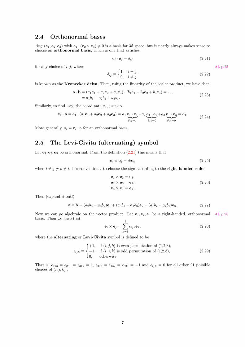
2.4 Orthonormal bases
Any (e1, e2, e3) with e1 · (e2 × e3) 6= 0 is a basis for 3d space, but it nearly always makes sense tochoose an orthonormal basis, which is one that satisfies
ei · ej = δij (2.21)
for any choice of i, j, where AL p.25
δij ≡{
1, i = j,
0, i 6= j,(2.22)
is known as the Kronecker delta. Then, using the linearity of the scalar product, we have that
a · b = (a1e1 + a2e2 + a3e3) · (b1e1 + b2e2 + b3e3) = · · ·= a1b1 + a2b2 + a3b3.
(2.23)
Similarly, to find, say, the coordinate a1, just do
e1 · a = e1 · (a1e1 + a2e2 + a3e3) = a1 e1 · e1︸ ︷︷ ︸δ11=1
+a2 e1 · e2︸ ︷︷ ︸δ12=0
+a3 e1 · e3︸ ︷︷ ︸δ13=0
= a1.(2.24)
More generally, ai = ei · a for an orthonormal basis.
2.5 The Levi-Civita (alternating) symbol
Let e1, e2, e3 be orthonormal. From the definition (2.21) this means that
ei × ej = ±ek (2.25)
when i 6= j 6= k 6= i. It’s conventional to choose the sign according to the right-handed rule:
e1 × e2 = e3,
e2 × e3 = e1,
e3 × e1 = e2.
(2.26)
Then (expand it out!)
a× b = (a2b3 − a3b2)e1 + (a3b1 − a1b3)e2 + (a1b2 − a2b1)e3. (2.27)
Now we can go algebraic on the vector product. Let e1, e2, e3 be a right-handed, orthonormal AL p.25basis. Then we have that
ei × ej =
3∑k=1
εijkek, (2.28)
where the alternating or Levi-Civita symbol is defined to be
εijk ≡
+1, if (i, j, k) is even permutation of (1,2,3),
−1, if (i, j, k) is odd permutation of (1,2,3),
0, otherwise.
(2.29)
That is, ε123 = ε231 = ε312 = 1, ε213 = ε132 = ε321 = −1 and εijk = 0 for all other 21 possiblechoices of (i, j, k) .
7

Now we can easily express vector equations in terms of their coordinates:
r = p + λq → ri = pi + λqi,
d = a · b → d =
3∑i=1
aibi,
c = a× b → ci =
3∑j=1
3∑k=1
εijkajbk,
a · (b× c) →3∑i=1
3∑j=1
3∑k=1
εijkaibjck.
Exercises
1. Show that a · (a× c) = 0.
2. Show that the triple product a · (b× c) is unchanged under cyclic interchange of a,b, c. Corrected from a×(b × c)!
3. Use the (important) identity AL p.25
3∑i=1
εijkεilm = δjlδkm − δjmδkl, (2.30)
to show that
3∑i=1
3∑j=1
εijkεijm = 2δkm,
3∑i=1
3∑j=1
3∑k=1
εijkεijk = 6,
(2.31)
and to prove the following relations involving the vector product: AL p.26
a× (b× c) = (a · c)b− (a · b)c,
(a× b) · (c× d) = (a · c)(b · d)− (a · d)(b · c),
a · (a× b) = 0.
(2.32)
8
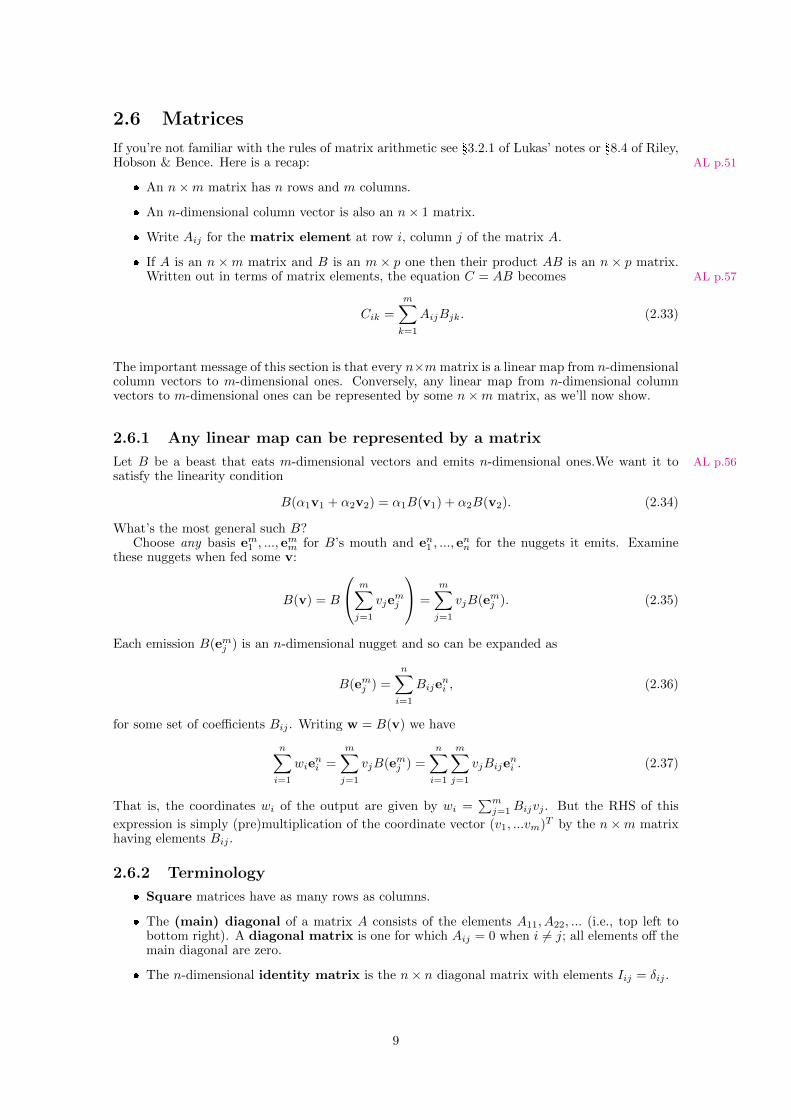
2.6 Matrices
If you’re not familiar with the rules of matrix arithmetic see §3.2.1 of Lukas’ notes or §8.4 of Riley,Hobson & Bence. Here is a recap: AL p.51
� An n×m matrix has n rows and m columns.
� An n-dimensional column vector is also an n× 1 matrix.
� Write Aij for the matrix element at row i, column j of the matrix A.
� If A is an n ×m matrix and B is an m × p one then their product AB is an n × p matrix.Written out in terms of matrix elements, the equation C = AB becomes AL p.57
Cik =
m∑k=1
AijBjk. (2.33)
The important message of this section is that every n×m matrix is a linear map from n-dimensionalcolumn vectors to m-dimensional ones. Conversely, any linear map from n-dimensional columnvectors to m-dimensional ones can be represented by some n×m matrix, as we’ll now show.
2.6.1 Any linear map can be represented by a matrix
Let B be a beast that eats m-dimensional vectors and emits n-dimensional ones.We want it to AL p.56satisfy the linearity condition
B(α1v1 + α2v2) = α1B(v1) + α2B(v2). (2.34)
What’s the most general such B?Choose any basis em1 , ..., e
mm for B’s mouth and en1 , ..., e
nn for the nuggets it emits. Examine
these nuggets when fed some v:
B(v) = B
m∑j=1
vjemj
=
m∑j=1
vjB(emj ). (2.35)
Each emission B(emj ) is an n-dimensional nugget and so can be expanded as
B(emj ) =
n∑i=1
Bijeni , (2.36)
for some set of coefficients Bij . Writing w = B(v) we have
n∑i=1
wieni =
m∑j=1
vjB(emj ) =
n∑i=1
m∑j=1
vjBijeni . (2.37)
That is, the coordinates wi of the output are given by wi =∑mj=1Bijvj . But the RHS of this
expression is simply (pre)multiplication of the coordinate vector (v1, ...vm)T by the n×m matrixhaving elements Bij .
2.6.2 Terminology
� Square matrices have as many rows as columns.
� The (main) diagonal of a matrix A consists of the elements A11, A22, ... (i.e., top left tobottom right). A diagonal matrix is one for which Aij = 0 when i 6= j; all elements off themain diagonal are zero.
� The n-dimensional identity matrix is the n× n diagonal matrix with elements Iij = δij .
9

� Given an n×m matrix A, its transpose AT is the m×n matrix with elements [AT ]ij = Aji.Its Hermitian conjugate A† has elements [A†]ij = A?ji.
� If AT = A then A is symmetric. If A† = A it is Hermitian.
� If AAT = ATA = I then A is orthogonal. If AA† = A†A = I then A is unitary.
� Suppose A and B are both n× n matrices. Then in general AB 6= BA. The difference
[A,B] ≡ AB −BA (2.38)
is called the commutator of A and B. It’s another n× n matrix. If it is equal to the n× n AL p.59zero matrix then A and B are said to commute.
Exercises
1. A 2× 2 matrix is a linear map from the plane (2d column vectors) onto itself. It is completelydefined by 4 numbers. Identify the different types of transformation that can be constructedfrom these 4 numbers.
2. A 3 × 3 matrix maps 3d space onto itself. It has 9 free parameters. Identify the geometricaltransformations that it can effect.
3. Given a n× n matrix with complex coefficients, how to characterise the map it represents?
4. Show that (AB)T = BTAT and (AB)† = B†A†. Hence show that AAT = I implies ATA = I.
5. Show that the map B(x) = n× x is linear. Find the find the matrix that represents it. AL p.57
10
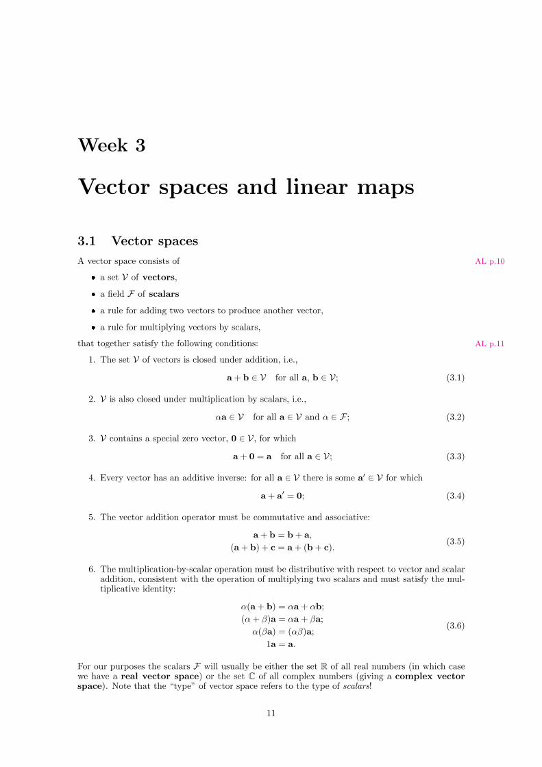
Week 3
Vector spaces and linear maps
3.1 Vector spaces
A vector space consists of AL p.10
� a set V of vectors,
� a field F of scalars
� a rule for adding two vectors to produce another vector,
� a rule for multiplying vectors by scalars,
that together satisfy the following conditions: AL p.11
1. The set V of vectors is closed under addition, i.e.,
a + b ∈ V for all a, b ∈ V; (3.1)
2. V is also closed under multiplication by scalars, i.e.,
αa ∈ V for all a ∈ V and α ∈ F ; (3.2)
3. V contains a special zero vector, 0 ∈ V, for which
a + 0 = a for all a ∈ V; (3.3)
4. Every vector has an additive inverse: for all a ∈ V there is some a′ ∈ V for which
a + a′ = 0; (3.4)
5. The vector addition operator must be commutative and associative:
a + b = b + a,
(a + b) + c = a + (b + c).(3.5)
6. The multiplication-by-scalar operation must be distributive with respect to vector and scalaraddition, consistent with the operation of multiplying two scalars and must satisfy the mul-tiplicative identity:
α(a + b) = αa + αb;
(α+ β)a = αa + βa;
α(βa) = (αβ)a;
1a = a.
(3.6)
For our purposes the scalars F will usually be either the set R of all real numbers (in which casewe have a real vector space) or the set C of all complex numbers (giving a complex vectorspace). Note that the “type” of vector space refers to the type of scalars!
11
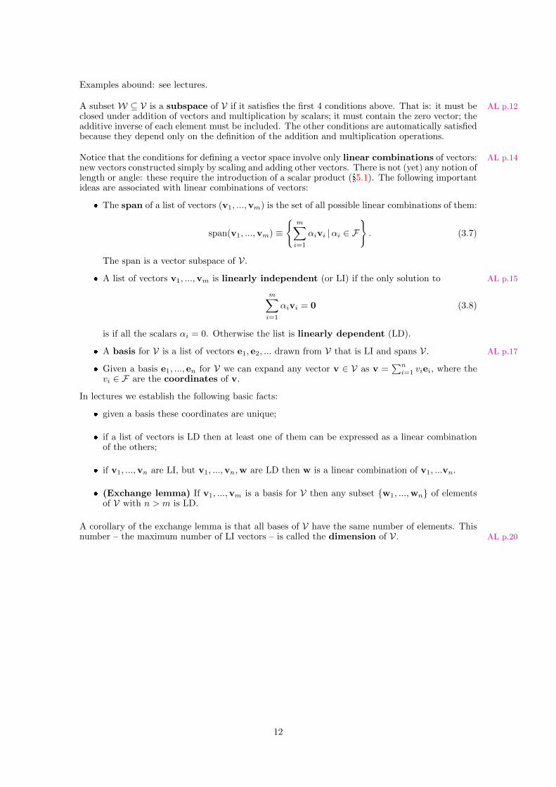
Examples abound: see lectures.
A subset W ⊆ V is a subspace of V if it satisfies the first 4 conditions above. That is: it must be AL p.12closed under addition of vectors and multiplication by scalars; it must contain the zero vector; theadditive inverse of each element must be included. The other conditions are automatically satisfiedbecause they depend only on the definition of the addition and multiplication operations.
Notice that the conditions for defining a vector space involve only linear combinations of vectors: AL p.14new vectors constructed simply by scaling and adding other vectors. There is not (yet) any notion oflength or angle: these require the introduction of a scalar product (§5.1). The following importantideas are associated with linear combinations of vectors:
� The span of a list of vectors (v1, ...,vm) is the set of all possible linear combinations of them:
span(v1, ...,vm) ≡
{m∑i=1
αivi |αi ∈ F
}. (3.7)
The span is a vector subspace of V.
� A list of vectors v1, ...,vm is linearly independent (or LI) if the only solution to AL p.15
m∑i=1
αivi = 0 (3.8)
is if all the scalars αi = 0. Otherwise the list is linearly dependent (LD).
� A basis for V is a list of vectors e1, e2, ... drawn from V that is LI and spans V. AL p.17
� Given a basis e1, ..., en for V we can expand any vector v ∈ V as v =∑ni=1 viei, where the
vi ∈ F are the coordinates of v.
In lectures we establish the following basic facts:
� given a basis these coordinates are unique;
� if a list of vectors is LD then at least one of them can be expressed as a linear combinationof the others;
� if v1, ...,vn are LI, but v1, ...,vn,w are LD then w is a linear combination of v1, ...vn.
� (Exchange lemma) If v1, ...,vm is a basis for V then any subset {w1, ...,wn} of elementsof V with n > m is LD.
A corollary of the exchange lemma is that all bases of V have the same number of elements. Thisnumber – the maximum number of LI vectors – is called the dimension of V. AL p.20
12
3.2 Linear maps
Recall that a function is a mapping f : X → Y from a set X (the domain of f) to another set Y AL p.42(the codomain of f). The image of f is defined as
Im f ≡ {f(x)|x ∈ X} ⊆ Y. (3.9)
The map f is
� one-to-one (injective) if each y ∈ Y is mapped to by at most one element of X;
� onto (surjective) if each y ∈ Y is mapped to by at least one element of X;
� bijective if each y ∈ Y is mapped to by precisely one element of X (i.e., f is both injectiveand surjective).
A trivial but important map is the identity map,
idX : X → X,
defined by idX(x) = x. Given f : X → Y and g : Y → Z we define their composition g ◦ f :X → Z as the new map, AL p.43
(g ◦ f)(x) = g(f(x)),
obtained by applying f first, then g to the result. A map g : Y → X is the inverse of f : X → Yif f ◦ g = idY and g ◦ f = idX . If it exists this inverse map is usually written as f−1. It is a fewlines’ work to prove the following fundamental properties of inverse maps:
� f is invertible ⇔ f is bijective. The inverse function is unique. AL p.44
� if f : X → Y and h : Y → Z are both invertible then (h ◦ f)−1 = f−1 ◦ h−1;
� (f−1)−1 = f .
For the rest of the course we’ll focus on maps f : V → W, whose domain V and codomain W arevector spaces, possibly of different dimensions, but over the same field F . Such an f : V → W is AL p.45linear if for all vectors v1,v2 ∈ V and all scalars α ∈ F ,
f(v1 + v2) = f(v1) + f(v2),
f(αv) = αf(v).(3.10)
It’s easy to see from that that if f : V → W and g : W → U are both linear maps then theircomposition g ◦ f : V → U is also linear. And if a linear f : V → V is bijective then its inverse f−1
is also a linear map.
3.2.1 Properties of linear maps
The kernel of f is the set of all elements v ∈ V for which f(v) = 0. The rank of f is the dimension AL p.45of its image.
Ker f ≡ {v ∈ V | f(v) = 0},rank f ≡ dim Im f.
(3.11)
Directly from these definitions we have that AL p.46
� f(0) = 0. Therefore 0 ∈ Ker f .
� Ker f is a vector subspace of V.
� Im f is a vector subspace of W.
� f surjective ⇔ Im f = W ⇔ dim Im f = dimW.
13
� f injective ⇔ Ker f = {0} ⇔ dim Ker f = 0.
But the main result in this section is that any linear map f : V → W satisfies the dimensiontheorem AL p.47
dim Ker f + dim Im f = dimV. (3.12)
We’ll be invoking this theorem over the next few lectures. Here are some immediate consequences
of it:
� if f has an inverse (bijective) then dimV = dimW; AL p.48
� if dimV = dimW then the following statements are equivalent (they are all either true orfalse): f is bijective ⇔ dim Ker f = 0⇔ rank f = dimW;
3.2.2 Examples of linear maps
� Matrices Any n×m matrix is a linear map from Fm to Fn: for any u,v ∈ Fm we have AL p.49that A(u + v) = A(u) +A(v) and A(αv) = α(Av). Composition is multiplication.
� Coordinate maps Given a vector space V over a field F with basis e1, ..., en, we have thatany vector in V can be expressed as
v =
n∑i=1
viei,
where the vi are the coordinates of the vector wrt the ei basis. Introduce a mapping ϕ :Fn → V defined by
ϕ
v1...vn
=
n∑i=1
viei. (3.13)
This is called the coordinate map (for the basis e1, ..., en). It is clearly linear. BecausedimFn = dimV and Imϕ = V it follows as a consequence of the dimension theorem that ϕis bijective and therefore has an inverse mapping ϕ−1 : V → Fn. The coordinates (v1, ...., vn)of the vector v are simply ϕ−1(v), the ith element of which is vi. typo removed
� Linear differential operators Consider the vector space C∞(R) of smooth functionsf : R→ C. Then the differential operator
L : C∞(R)→ C∞(R)
L• =
n∑i=0
pi(x)di
dxi• (3.14)
is a linear map.
14
3.3 Change of basis of the matrix representing a linear map
Let f : V → W be a linear map. Suppose that v1, ...,vm is a basis for V with coordinate map AL p.71φ : Fm → V, and w1, ...,wn is a basis for W with coordinate map ψ : Fn → W. The matrix Athat represents f : V → W in these bases is simply
A = ψ−1 ◦ f ◦ φ. (3.15)
Now consider another pair of bases for V and W with coordinate maps
ϕ′ : Fm → V, basis v′1, ...,v′m ∈ V;
ψ′ : Fn →W, basis w′1, ...,w′n ∈ W.
The matrix A′ representing f : V → W in the new primed bases is given by
A′ = (ψ′)−1 ◦ f ◦ ϕ′
= (ψ′)−1 ◦ ψ︸ ︷︷ ︸Q
◦ψ−1 ◦ f ◦ ϕ︸ ︷︷ ︸A
◦ϕ−1 ◦ ϕ′︸ ︷︷ ︸P−1
. (3.16)
Here P−1 is an m ×m matrix that transforms coordinate vectors wrt the v′i basis to the vi one.Inverting, P transforms unprimed coordinates to primed ones. Similarly, Q transforms from thewi basis to the w′i one.
The most important case is when V = W, vi = wi, v′i = w′i. Then A and A′ are both squareand are related through
A′ = PAP−1. (3.17)
Here’s how this works: P−1 transforms coordinate vectors from the primed to unprimed basis.Then A acts on that before we transform the resulting coordinates back to the primed basis.Think P does the priming of the coordinates!
Exercises
1. We have just seen that coordinate vectors α = (α1, ..., αm)T and α′ = (α′1, ..., α′m)T with
respect to these two bases are related via α′ = Pα, or, in index form, α′j =∑k Pjkαk. Show
that the basis vectors transform in the opposite way: vj =∑k(P−1)jkv
′k.
2. Consider the reflection matrix A =
(1 00 −1
). What is the corresponding matrix in a new
basis rotated counterclockwise by α: v′1 =
(cosαsinα
), v′2 =
(− sinαcosα
)?
15
Week 4
More on matrices and maps
4.1 Systems of linear equationsAL p.73
Suppose we have n simultaneous equations in m unknowns:
A11x1 + · · ·A1mxm = b1,
......
An1x1 + · · ·Anmxm = bn.
(4.1)
In matrix form this is Ax = b, where A is an n×m matrix, b is an n-dimensional column vectorand x is the m-dimensional column vector we’re trying to find. If b = 0 the system of equationsis called homogeneous.
Exercises
1. Show that the full space of solutions to Ax = b is the set {x0 + x1 |x0 ∈ kerA}, where x1 isany vector for which Ax1 = b.
4.1.1 Rows versus columnsAL p.54
AL p.74In §3.2.1 (eq. 3.11) we defined the rank of a linear map as being equal to the dimension of itsimage. Here we distinguish between the row rank and the column rank of a matrix and show thatthey are in fact equal.
We’ll need the following result. LetW be a vector subspace of Fm. The orthogonal complementto W is
W⊥ ≡ {v |v ·w = 0, for all w ∈ W,v ∈ Fm}, (4.2)
in which v ·w =∑mi=1 viwi.
1 The orthogonal complement dimension theorem states that AL p.100
dimW + dimW⊥ = m. (4.3)
The proof is similar to that for the original dimension theorem (3.12).
Now let’s apply this to matrices. We can view the n×m matrix A as either
1. m column vectors, A1, ...,Am (each having n entries), or
2. n row vectors A1, ...An (each having m entries).
These lead to two different ways of thinking about solutions to the inhomogeneous equation Ax = 0:
1In §6.4 we’ll recycle this idea, but replacing the v · w in the definition of W† by the scalar product 〈v,w〉.Equation (4.3) still holds for this modified definition of W⊥.
16

1. The solution space is simply kerA, i.e., everything that doesn’t map to ImA\{0}. Thisunmapped space is ImA = span(A1, ...,Am), the span of the columns of A. By the (original)dimension theorem (3.12) we have
column rank︸ ︷︷ ︸dim ImA
+ dim space of solns︸ ︷︷ ︸dimKerA
= m. (4.4)
2. Consider instead the n rows of A. The vector equation Ax = 0 is equivalent to the n scalarequations Ai · x = 0, where · is matrix multiplication as used in the definition (4.2) of W⊥above. That is, solutions live in the space “orthogonal” to that spanned by the rows. Let Wbe the vector subspace of Fm spanned by the row vectors A1, ...,An. Its dimension is therow rank of A. W⊥ is then the space of solutions to Ai · v = 0 (i = 1, ..., n). From theorthogonal complement dimension theorem (4.3),
row rank︸ ︷︷ ︸dimW
+ dim space of solns︸ ︷︷ ︸dimW⊥
= m. (4.5)
Comparing (4.4) and (4.5) shows that the row rank is equal to the (column) rank. [Lukas p.55]
4.1.2 How to calculate the rank of a matrixAL p.63
That’s wonderful, but given a matrix how do we actually calculate its rank? To do this observethat the vector subspace spanned by a list of vectors v1, ...,vn ∈ V is unchanged if we perform anysequence of the following operations:
� Swap any pair vi and vj ;
� Multiply any vi by a nonzero scalar;
� Replace vi by vi + αvj .
We can apply these operations to the rows A1,A2, ... of A to reduce it to a form from which wecan read off the row rank by inspection. For example, if A is a 5× 5 matrix and we reduce it to
(A1)1 (A1)2 (A1)3 (A1)4 (A1)50 (A2)2 (A2)3 (A2)4 (A2)50 0 (A3)3 (A3)4 (A3)50 0 0 0 (A4)50 0 0 0 0
then it’s clear that the (row) rank of A is 4. This procedure is called row reduction: the idea isto reduce the matrix to so-called row echelon form in which the first nonzero element of row iis rightwards of the first nonzero element of the preceding row i− 1. 2
4.1.3 How to solve systems of linear equations: Gaussian eliminationAL p.63
Row reduction is based on the invariance of rankA under the following elementary row opera-tions:
� Swap two rows Ai, Aj ;
� Multiply any Ai by a nonzero value;
� Add αAj to Ai.
Each of these operations has a corresponding elementary matrix. For example, to add αA1 toA2 we can premultiply A by 1 0 0 0
α 1 0 00 0 1 00 0 0 1
. (4.6)
2Because row rank=column rank we could just as well apply the same idea to A’s columns, but it’s conventionalto use rows.
17

To solve Ax = b we can premultiply both sides by a sequence of elementary matrices E1, E2, ...,Ek, reducing it to
(Ek · · ·E2E1A)x = (Ek · · ·E2E1)b, (4.7)
in which the matrix (Ek · · ·E2E1A) on the LHS is reduced to row echelon form. That is,
1. Use row reduction to bring A into echelon form; AL p.77
2. apply the same sequence of row operations to b;
3. solve for x by backsubstitution.
The advantage of this procedure over other methods (e.g., using the inverse) is that we can constructkerA and deal with the case when the solution is not unique.
4.1.4 How to find the inverse of a matrixAL p.66
We can use the same idea to construct the inverse A−1 of A (if it exists, or, if doesn’t, to diagnosewhy not). The steps are as follows:
0. Stop! Do you really need to know A−1? For example, it is better to use row reduction tosolve Ax = b than to try to apply A−1 to both sides.
1. Apply row-reduction operations to eliminate all elements of A below the main diagonal.
2. Apply row-reduction operations to eliminate all elements of A above the main diagonal.
3. Apply the same sequence of operations to the identity matrix I. The result will be A−1.
How does this work? In reducing A to the identity matrix we are implicitly finding a sequence ofelementary matrices E1, ..., Ek for which
Ek · · ·E2E1A = I. (4.8)
From this it follows that the inverse is given by
A−1 = Ek · · ·E2E1I. (4.9)
Exercises
1. Use row reduction operations to obtain the rank and kernel of the matrix(0 1 −12 3 −22 1 0
). (4.10)
2. Solve the system of linear equations
y − z = 1,
2x+ 3y − 2z = 1,
2x+ y = b.
(4.11)
3. Find the inverse of the matrix (1 1 22 −1 101 −2 3
)(4.12)
4. Given a matrix A explain how to find kerA. Find kerA for
A =
(1 2 34 5 67 8 9
)(4.13)
18

Another, less efficient, way of calculating A−1 is by using the Laplace expansion of the determinant,equation (4.2.3) below.
19
4.2 Determinant
Suppose V1, ...,Vk are vector spaces over a common field of scalars F . A map f : V1×· · ·×Vk → Fis multilinear, specifically k-linear, if it is linear in each argument separately: AL p.82
f(v1, ..., αvi + α′v′i, ...,vk) = αf(v1, ...,vi, ...,vk) + α′f(v1, ...,v′i, ...,vk). (4.14)
For the special case k = 2 the map is called bilinear. A multilinear map is alternating if it returnszero whenever two of its arguments are equal:
f(v1, ...,vi, ...,vi, ...,vk) = 0. (4.15)
This means that swapping any pair of arguments to a alternating multilinear map flips the sign ofits output.
4.2.1 Definition of the determinant
The determinant is the (unique) mapping from n×nmatrices to scalars that is n-linear alternatingin the columns, and takes the value 1 for the identity matrix. It directly follows that:
1. If two columns of A are identical then detA = 0.
2. Swapping two columns of A changes the sign of detA.
3. If B is obtained from A by multiplying a single column of A by a factor c then detB = cdetA.
4. If one column of A consists entirely of zeros then detA = 0.
5. Adding a multiple of one column to another does not change detA.
4.2.2 The Leibniz expansion of the determinant
We can express each column Aj of the matrix A as a linear combination Aj =∑iAijei of the
column basis vectors e1 = (1, 0, 0, ..)T , ..., en = (0, .., 0, 1)T . For any k-linear map δ we have that,by definition,
δ(A1, ...,Ak) = δ
(n∑
i1=1
Ai1,1ei1 , ...,
n∑ik=1
Aik,keik
)=
n∑i1=1
· · ·n∑
ik=1
Ai1,1 · · ·Aik,kδ(ei1 , ..., eik),
showing that the map is completely determined by the nk possible results of applying it to thebasis vectors. Imposing the condition that δ be alternating means that that δ(ei1 , ..., ein) vanishesif two or more of the ik are equal. Therefore we need consider only those (i1, ..., in) that arepermutations P of the list (1, ..., n). The change of sign under pairwise exchanges implied by thealternating condition means that
δ(eP (1), ..., eP (n)) = sgn(P )δ(e1, ..., en),
where sgn(P ) = ±1 is the sign of the permutation P (+1 for even, −1 for odd). Finally thecondition that det I = 1 sets δ(e1, ..., en) = 1, completely determining δ. The result is that AL p.84
detA =∑P
sgn(P )AP (1),1AP (2),2 · · ·AP (n),n
=
n∑i1=1
· · ·n∑
in=1
εi1,...,inAi1,1 · · ·Ain,n,(4.16)
where εi1,...,in is the multidimensional generalisation of the Levi-Civita or alternating symbol (4.15).
There are two important results that follow hot on the heels of the Leibniz expansion: AL p.86
� det(AT) = detA
– This implies that the determinant is also multilinear and alternating in the rows of A.
20
� det(AB) = (detA)(detB)
– From this it follows that A is invertible iff detA 6= 0. Moreover, det(A−1) = 1/detA.
– The determinant of the matrix that represents a linear map is independent of basis used:in another basis the matrix representing the map becomes A′ = PAP−1 (equ. 3.17) andso detA′ = detA. As every linear map is represented by some matrix, this meansthat we can sensibly extend our definition of determinant to include any linear mapf : V → V.
4.2.3 Laplace’s expansion of the determinantAL p.88
Although the Leibniz expansion (4.16) of detA is probably unfamiliar to you, you are likely tohave encountered its Laplace expansion, which we now summarise. Given an n× n matrix A, letA(i,j) be the (n−1)× (n−1) matrix obtained by omitting the ith row and jth column of A. Definethe cofactor matrix as
cij = (−1)i+j det(A(i,j)). (4.17)
Its transpose is known as the adjugate matrix or classical adjoint of A:
(adjA)ji = (−1)i+j det(A(i,j)). (4.18)
Then with some work we can show from the Leibniz expansion that
δij detA =
n∑k=1
Aikcjk =
n∑k=1
ckiAkj , (4.19)
or, in matrix notation,(detA)I = A adjA = (adjA)A, (4.20)
where I is the n× n identity matrix. This is known as the Laplace expansion of the determinant.An immediate corollary is an explicit expression for the inverse of a matrix: AL p.90
A−1 =1
detAadjA.
4.2.4 Geometrical meaning of the determinant
detA is the (oriented) n-dimensional volume of the n-dimensional parallelpiped spanned by thecolumns (or rows) of A. See, e.g., XX,§4 of Lang’s Undergraduate analysis for the details.
4.2.5 A standard application of determinants: Cramer’s rule
Consider the set of simultaneous equation Ax = b. For each i = 1, ..., n introduce a new matrix AL p.91
B(i) = (A1, ...,A(i−1),b,A(i+1), ...An),
obtained by replacing column i in A with b. Note that because Ax = b we have b =∑j xjA
j .So, using the multilinearity property of the determinant,
det(B(i)) = det(A1, ...,A(i−1),b,A(i+1), ...An)
= det(A1, ...,A(i−1),
∑xjA
j ,A(i+1), ...An)
=∑j
xj det(A1, ...,A(i−1),Aj ,A(i+1), ...An
)=∑j
xjδij detA = xi detA,
(4.21)
21

the last line following because the determinants vanish unless i = j. This shows that we may solveAx = b in a cute but inefficient matter by calculating
xi = det(B(i))/ detA (4.22)
for each i = 1, ..., n.
22
4.3 Trace
The trace of an n× n matrix A is defined to be the sum of its diagonal elements: AL p.110
trA ≡n∑i=1
Aii. (4.23)
Exercises
1. Show that
tr(AB) = tr(BA),
tr(ABC) = tr(CAB).(4.24)
2. Let A and A′ be matrices that represent the same linear map in two different bases. Show thattrA′ = trA.
3. Show that the trace of any matrix that represents a rotation by an angle θ in 3d space is equalto 1 + 2 cos θ.
23
Week 5
Scalar product, dual vectors andadjoint maps
5.1 Scalar product
Our definition (§3.1) of vector space relies only on the most fundamental idea of taking linearcombinations of vectors. By introducing a scalar product (also known as an inner product) betweenpairs of vectors we can extend our algebraic manipulations to include lengths and angles.
Formally, a scalar product 〈•, •〉 on a vector space V is a mapping V ×V → F between pairs ofvectors and scalars that satisfies the following conditions: AL p.93
〈c, αa + βb〉 = α〈c,a〉+ β〈c,b〉 (linear in second argument) (5.1)
〈b,a〉 = 〈a,b〉? (swapping conjugates) (5.2)
〈a,a〉 = 0, iff a = 0,
> 0, otherwise. (positive definite) (5.3)
Comments:
� if V is a real vector space then the scalar product is real.
� if V is a complex vector space then the scalar product is complex.
� Condition (5.2) guarantees that 〈a,a〉 ∈ R. Together with (5.3) this means that we can definethe length (or magnitude or norm) |a| of the vector a through
|a|2 = 〈a,a〉. (5.4)
Similarly in real vector spaces we define the angle θ between nonzero vectors a and b via
〈a,b〉 = |a| |b| cos θ, (5.5)
and say that they are orthogonal if
〈a,b〉 = 0. (5.6)
� Using conditions (5.1) and (5.2) together we have that
〈αa + βb, c〉 = α?〈a, c〉+ β?〈b, c〉. (5.7)
That is, 〈•, •〉 is linear in the first argument only for real vector spaces!
Some examples of scalar products: AL p.94
� For Cn, the space of n-dimensional vectors with complex coefficients the natural scalar prod-uct is
〈a,b〉 = a† · b =
n∑i=1
a?i bi. (5.8)
24

� For the space L2(a, b) of square-integrable functions f : [a, b]→ C the natural choice is
〈f, g〉 =
∫ b
a
f?(x)g(x) dx. (5.9)
� There is one important exception to these rules in undergraduate physics. In relativitythe metric defines a scalar product between pairs of tangent vectors in four-dimensionalspacetime in which the positive-definiteness condition (5.3) is relaxed. Spacetime is a realvector space, which means that only the linearity condition (5.1) matters. In this course,however, we’ll demand positive definiteness.
Exercises
1. Consider a generalisation of (5.8) to
〈a,b〉 = a†Mb =
n∑i,j=1
a?iMijbj . (5.10)
where M is an n × n matrix. This gives us linearity in b (5.1) for free. What constraints dothe other two conditions, (5.2) and (5.3), impose on M?
2. [For your second pass through the notes:] In the definition (5.5) of the angle θ between twovectors how do we know that | cos θ| ≤ 1?
3. If the nonzero v1, ...,vn are pairwise orthogonal (that is 〈vi,vj〉 = 0 for i 6= j) show that they AL p.95must be LI.
4. Show that if 〈v,w〉 = 0 for all v ∈ V then w = 0. AL p.99
5. Suppose that the maps f : V → V and g : V → V satisfy
〈v, f(w)〉 = 〈v, g(w)〉 (5.11)
for all v,w ∈ V. Show that f = g. (Do not assume that f and g are linear maps.)
5.1.1 Important relations involving the scalar product
|a + b|2 = |a|2 + |b|2 if 〈a,b〉 = 0 (Pythagoras) (5.12)
|a + b|2 + |a− b|2 = 2(|a|2 + |b|2
)(Parallelogram Law) (5.13)
|〈a,b〉|2 ≤ |a|2|b|2 (Cauchy–Schwarz inequality) (5.14)
|a + b| ≤ |a|+ |b| (Triangle inequality). (5.15)
AL p.22
5.1.2 Orthonormal bases
An orthonormal basis for V is a set of basis vectors e1, ..., en that satisfy AL p.95
〈ei, ej〉 = δij . (5.16)
Referred to such an orthonormal basis,
� the coordinates of a are given byaj = 〈ej ,a〉; (5.17)
� in terms of these coordinates the scalar product becomes
〈a,b〉 =
n∑i=1
a?i bi; (5.18)
25

� identifying e1, e2, ... with the column vectors (1, 0, 0, ..)T , (0, 1, 0, 0, ...)T etc, the matrix Mthat represents a linear map f : V → V has matrix elements
Mij = 〈ei, f(ej)〉. (5.19)
Given a list v1, ...,vm of vectors we can construct an orthonormal basis for their span using thefollowing, known as the Gram–Schmidt algorithm: AL p.97
1. Choose one of the vectors v1. Let e′1 = v1. Our first basis vector is e1 = e′1/|e′1|.
2. Take the second vector v2 and let e′2 = v2−〈e1, e2〉e1: that is, we subtract off any componentthat is parallel to e1. If the result is nonzero then our second normalized basis vector ise2 = e′2/|e′2|.
3. ...
k. By the kth step we’ll have constructed e1, ...ej for some j ≤ k. Subtract off any component
of vk that is parallel to any of these: e′k = vk −∑j−1i=1 〈ei,vk〉ei. If e′k 6= 0 then our next
basis vector is ej+1 = e′k/|ve′k|.
Exercises
1. Construct an orthnormal basis for the space spanned by the vectors v1 =(
110
), v2 =
(201
),
v3 =(
1−2−2
).
26
5.2 Adjoint map
Let f : V → V be a linear map. Its adjoint f† : V → V is defined as the map that satisfies AL p.100
〈f†(u),v〉 = 〈u, f(v)〉. (5.20)
Directly from this definition we have that
� f† is unique. Suppose that both f† = f1 and f† = f2 satisfy (5.20). Then
〈f1(u),v〉 = 〈u, f(v)〉 = 〈f2(u),v〉. (5.21)
Then using (5.2) together with the result of exercise 5 we have that f1 = f2.
� f† is a linear map. Setting u = α1u1 + α2u2 in (5.20) and taking the complex conjugategives ⟨
v, f†(α1u1 + α2u2)⟩
=〈f(v), α1u1 + α2u2〉= α1〈f(v),u1〉+ α2〈f(v),u2〉= α1
⟨v, f†(u1)
⟩+ α2
⟨v, f†(u2)
⟩⟨v, f†(α1u1 + α2u2)− α1f
†(u1)− α2f†(u2)
⟩= 0.
(5.22)
Then by the result of exercise 4 it follows that
f†(α1u1 + α2u2) = α1f†(u1) + α2f
†(u2). (5.23)
� f† has the following properties:
(f†)† = f (5.24)
(f + g)† = f† + g† (5.25)
(αf)† = α?f (5.26)
(f ◦ g)† = g† ◦ f† (5.27)
(f−1)† = (f†)−1 (assuming f invertible) (5.28)
Suppose that A is the matrix that represents f in some orthonormal basis e1, ..., en. Then by(5.19), (5.20) and (5.2) the matrix A† that represents f† in the same basis has elements
(A†)ij =⟨ei, f
†(ej)⟩
= A?ji. (5.29)
That is, A† is the Hermitian conjugate of A.
27

5.3 Hermitian, unitary and normal maps
A Hermitian operator f : V → V is one that is self-adjoint: AL p.101
f† = f. (5.30)
The corresponding matrices satisfy A = A†, or, more explicitly,
Aij = A?ji. (5.31)
If V is a real vector space then the matrix A is symmetric.A unitary operator f : V → V preserves scalar products: AL p.102
〈f(u), f(v)〉=〈u,v〉. (5.32)
[If V is a real vector space then orthogonal is more often used.] Using (5.20) the condition (5.32)can also be written as
⟨u, f†(f(v))
⟩=〈u,v〉. As this holds for any u,v an equivalent condition for
unitary is thatf ◦ f† = f† ◦ f = idV . (5.33)
That is, unitary operators satisfy f† = f−1. Taking the determinant of (5.33) we have
|det f |2 = 1. (5.34)
If f is an orthogonal map then this becomes det f = ±1. If det f = +1 then the map f is a purerotation. If det f = −1 then f is a rotation plus a reflection.
Let U be the matrix that represents a unitary map in some orthonormal basis. Then (5.33)becomes
n∑j=1
UijU?kj =
n∑j−1
U?jiUjk = δik. (5.35)
The first sum shows that the rows of U are orthonormal, the second its columns.
Hermitian and unitary maps are examples of so-called normal maps, which are those for which AL p.112
[f, f†] ≡ f ◦ f† − f† ◦ f = 0. (5.36)
Exercises
1. Let R be an orthogonal 3 × 3 matrix with detR = +1. How is trR related to the rotationangle?
2. Let U1 and U2 be unitary. Show that U2 ◦ U1 is also unitary. Does the commutator [U2, U1] ≡U2 ◦ U1 − U1 ◦ U2 vanish?
3. Suppose that H1 and H2 are Hermitian. Is H2 ◦ H1 also Hermitian? If not, are they anyconditions under which it becomes Hermitian?
28

5.4 Dual vector space
Let V be a vector space over the scalars F . The dual vector space V? is the set of all linearmaps ϕ : V → F : AL p.108
ϕ(α1v1 + α2v2) = α1ϕ(v1) + α2ϕ(v2). (5.37)
It is easy to confirm that the set of all such maps satisfies the vector space axioms (§3.1).Some examples of dual vectors spaces:
� If V = Rn, the space of real, n-dimensional column vectors, then elements of V? are real,n-dimensional row vectors.
� Take any vector space V armed with a scalar product 〈•, •〉. Then for any v ∈ V the mappingϕv(•) = 〈v, •〉 is a linear map from vectors • ∈ V to scalars. The dual space V? consists ofall such maps (i.e., for all possible choices of v).
In these examples dimV? = dimV. This is true more generally: just as we used the magic ofcoordinate maps to show that any n-dimensional vector space V over the scalars F is isomorphic1
to n-dimensional column vectors Fn, we can show that the dual space V? is isomorphic to thespace of n-dimensional row vectors. AL p.109When playing with dual vectors it is conventional to write elements of V and V? like so,
v =
n∑i=1
viei ∈ V,
ϕ =
n∑i=1
ϕiei? ∈ V?,
(5.38)
with upstairs indices for the coordinates vi of vectors in V, balanced by downstairs indices for thecorresponding basis vectors, and the other way round for V?.
1I don’t define what an isomorphism is in these notes, but do in the lectures. So look it up if you zoned out.
29
Week 6
Eigenthings
An eigenvector of a linear map f : V → V is any nonzero v ∈ V that satisfies the eigenvalueequation
f(v) = λv. (6.1)
The constant λ is the eigenvalue associated with v. AL p.113Some examples:
� Let R be a rotationg about some axis z. Clearly R leaves z unchanged. Therefore Rz = z.That is, z is an eigenvector of R with eigenvalue 1.
� The 2× 2 matrix
M =1√2
(1 11 1
)(6.2)
projects the (x, y) plane onto the line y = x. The vector ( 11 ) is a eigenvector with eigenvalue 1.
Another eigenvector is(−1
1
)with corresponding eigenvalue 0.
We can rewrtite the eigenvalue equation (6.1) as
(f − λ idV)(v) = 0. (6.3)
It has nontrivial solutions if rank(f − idV) < dimV, which is equivalent to AL p.114
det(f − λ idV) = 0, (6.4)
known as the characteristic equation for f . We define the eigenspace associated with theeigenvalue λ to be
Eigf (λ) ≡ ker(f − λ idV). (6.5)
30
6.1 How to find eigenvalues and eigenvectorsAL p.114
Choose a basis for V and let A be the n × n matrix that represents f in this basis. Then thecharacteristic equation (6.4) becomes
0 = det(A− λI) =∑Q
sgn(Q)(A− λI)Q(1),1) · · · (A− λI)Q(n),n, (6.6)
which is an nth-order polynomial equation for λ. Notice that
� This will have n roots, λ1, ..., λn, although some might be repeated.
� These roots (including repetitions) are the eigenvalues of A (and therefore of f).
� The eigenvalues are in general complex, even when V is a real vector space!
Having found λ1, ..., λn we can find each of the corresponding eigenvectors by constructing theeigenspace Eigλ(A) = ker(A − λiI). If for some λ the dimension m = dim ker(A − λI) > 1 thenthe eigenvalue λ is said to be (m-fold) degenerate or to have a degeneracy of m.
Exercises
1. Find the eigenvalues and eigenvectors of the following matrices:
1√2
(1 11 1
),
(0 −ii 0
),
(cos θ − sin θsin θ cos θ
),
(cos θ − sin θ 0sin θ cos θ 0
0 0 1
),
(1 10 1
). (6.7)
2. Show that detA =∏ni=1 λi and trA =
∑ni=1 λi.
3. Our procedure for finding the eigenvalues of f : V → V relies on choosing a basis for V andthen representing f as a matrix A. Show that the eigenvalues this returns are independent ofbasis used to construct the matrix.
31

6.2 Eigenproperties of Hermitian and unitary maps
The following statements are easy to prove. If f is a Hermitian map (f = f†) then AL p.119
� the eigenvalues of f are real, and
� the eigenvectors corresponding to distinct eigenvalues of f are orthogonal.
On the other hand, if f : V → V is a unitary map (f† = f−1) then AL p.123
� the eigenvalues of f are complex numbers with unit modulus, and
� the eigenvectors corresponding to distinct eigenvalues of f are orthogonal.
So, if the eigenvalues λ1, ..., λn of an n × n unitary or Hermitian matrix are distinct, then its n(normalized) eigenvectors are automatically an orthonormal basis.
6.3 DiagonalisationAL p.116
A map f : V → V is diagonalisable if there is a basis in which the matrix that represents f isdiagonal. An important lemma is that
f is diagonalisable ⇔ V has a basis of eigenvectors of f. (6.8)
Exercises
1. Now suppose that f is diagonalisable and let A be the n× n matrix that represents f in somebasis. According to the preceding lemma, this A has eigenvectors v1, ..vn with Avi = λivi thatform an eigenbasis for Cn. Let P = (v1, ...,vn) whose columns are these eigenvectors. Showthat
P−1AP = diag(λ1, ...λn). (6.9)
Diagonal matrices have such appealing properties (e.g., they commute, involve only n numbersinstead of n2) that we’d like to understand under what conditions a matrix representing a mapcan be diagonalised. The results of §6.2 imply that both Hermitian and unitary matrices arediagonalisable provided the eigenvalues are distinct. But we can do better than this. Next we’llshow that:
1. a map f is diagonalisable iff it is normal (5.36);
2. if we have two normal maps f1 and f2 then there is a basis in which the correspondingmatrices are simultaneously diagonal iff [f1, f2] = 0.
32
6.4 Eigenproperties of normal maps
Let f : V → V be a normal map (f ◦ f† = f† ◦ f). Then
� f(v) = λv⇒ f†(v) = λ?v; AL p.122
� V has an orthogonal basis of eigenvectors of f . AL p.123
It immediately follows that V has an orthonormal basis of eigenvectors of f .
Here is how this works in practice. If the eigenvalues of f are distinct then the eigenvectors areautomatically orthogonal. If there are degenerate eigenvalues (e.g., λ1 = λ2 then v1 and v2 are LIand span Eigf (λ), but aren’t necessarily orthogonal; we can use Gram–Schmidt to make them so.
In the v1, ...,vn eigenbasis the matrix D that represents f has elements
Dij =〈vi, f(vj)〉= λiδij . (6.10)
Now suppose that A is the matrix that represents f in our “standard” e1 = (1, 0, 0..)T , e2 =(0, 1, 0, ...)T etc basis. We can expand the eigenvectors vi =
∑j Qjiej : that is,
Q = (v1, ...,vn) (6.11)
is a matrix whose ith column is vi expressed in the standard e1, ..., en basis. Then
Q−1AQ = diag(λ1, ..., λn). (6.12)
Exercises
1. Diagonalise the matrix
A =1
2
(3 −1−1 3
). (6.13)
2. Diagonalize AL p.121
1
4
2 3√
2 3√
23√
2 −1 33√
2 3 −1
(6.14)
3. Show that if f has an orthonormal basis of eigenvectors then it is normal. [Hint: choose a basisand show that (A†)ij = A?ji.]
33

6.5 Simultaneous diagonalisation
Let A and B be two diagonalisable matrices. Then there is a basis in which both A and B arediagonalisable iff [A,B] = 0. AL p.125
34

6.6 Applications
� Exponentiating a matrix: AL p.129
exp[αG] = limm→∞
[I +
1
mαG
]m= In + αG+
1
2α2G2 + · · · =
∞∑j=0
1
j!(αG)j . (6.15)
If G is diagonalisable then G = P diag(λ1, ..., λn)P−1 and (6.15) becomes
exp[αG] = Pdiag(eαλ1 , ..., eαλn)P−1. (6.16)
� Quadratic forms. A quadratic form is an expression such as AL p.131
q(x, y, z) = ax2 + by2 + cz2 + dxy + eyz + fzx (6.17)
that is a sum of terms quadratic in the variables x, y, z. We can express any real quadraticform as
q(x1, ..., xn) =
n∑i=1
Q2iix
2i + 2
n∑i=1
i−1∑j=1
Qijxixj = xTQx, (6.18)
where x = (x1, ..., xn)rmT and Q is a symmetric matrix, Qij = Qji. Symmetric impliesdiagonalisability and so we can express Q = P diag(λ1, ..., λn)PT . In new coordinates x′ =PTx the quadratic form becomes
q(x) = q′(x′) = x′T diag(λ1, ..., λn)x′.λ1(x′1)2 + λ2(x′2)2 + · · ·+ λn(x′n)2, (6.19)
so that the level surfaces of q(x) (i.e., the solutions to q(x) = c for some constant level c)become easy to interpret geometrically.
Exercises
1. Calculate exp(αG) for G =(0 −11 0
).
2. Show thatdet expA = exp(trA). (6.20)
3. Sketch the solution to the equation 3x2 + 2xy + 2y2 = 1.
35