velocity boundary conditions for vorticity formulations …/67531/metadc681377/m2/1/high... ·...

*.-- - - I I

Velocity Boundary Conditions for Vorticity Formulations of the Incompressible Navier-Stokes Equations’

S.N. Kempka, J.H. Strickland, M.W. Glass, J.S. Peery Sandia National Laboratories

Albuquerque, NM

Prof. M.S. Ingber University of New Mexico

Albuquerque, NM

Abstract

Velocity boundary conditions for the vorticity form of the incompressible, viscous fluid momentum equations are presented. Vorticity is created on boundaries to simultaneously satisfy the tangential and normal components of the velocity boundary condition. The newly created vorticity is specified by a kinematical formulation which is a generalization of Helmholtz’ decomposition of a vector field. Related forms of the decomposition were developed by Bykhovskiy and Smirnov [5] in 1983, and Wu and Thompson [26] in 1973. Though it has not been generally recognized as such, these formulations resolve the over- specification issues associated with determining a velocity field from velocity boundary conditions and a vorticity field. The generalized decomposition has not been widely used, however, apparently due to a general lack of a useful physical interpretation. An analysis is presented which shows that the generalized decomposition has a relatively simple physical interpretation which facilitates its numerical implementation.

The implementation of the generalized decomposition for the normal and tangential velocity boundary conditions is discussed in detail. As an example of the use of this boundary condition, the flow in a lid-driven cavity is simulated. The solution technique is based on a Lagrangian transport algorithm in the hydrocode ALEGRE. ALEGRE’s Lagrangian transport algorithm has been modified to solve the vorticity transport equation, thus providing a new, accurate method to simulate incompressible flows. This numerical implementation and the new boundary condition formulation allow vorticity-based formulations to be used in a wider range of engineering problems.

1. This work was performed at Sandia National Laboratories supported by theU.S. Dept. of Energy under contract No. DE-AC04-94AL85000, and presented at the Forum on the Application of Vortex Methods to Engineering Problems, Albuquerque, NM, 87185, February, 2224,1995.

Introduction

A boundary condition for vorticity is required to solve the vorticity form of the Navier- Stokes equations for incompressible flows. Boundary conditions are typically specified in terms of velocities, however, so that vorticity boundary conditions must be deduced from the velocity boundary conditions. The vorticity boundary condition essentially represents the creation of vorticity whenever the tangential velocity on the boundary is specified, as in viscous flows.

Over the last two decades, many formulations for vorticity boundary conditions have been formulated, as described in reviews by Gresho [7], and Puckett [21]. Accurate flow simu- lations have been obtained using a wide variety of approaches, yet several fundamental issues remain to be resolved. Several previous models are described below.

Lighthill [15] proposed the basis for most approaches to describing vorticity creation. To begin, it is noted that the velocity induced by an arbitrary vorticity field (via the Biot-Sa- vart law) will not, in general, satisfy either the normal or tangential velocity boundary condition. A new velocity field which satisfies the normal velocity boundary condition can be obtained by adding a potential velocity field, which does not change the vorticity field. The tangential velocity boundary condition is not generally satisfied by the new velocity field, and the deviation from the boundary condition is generally referred to as a slip velocity, uslip. Lighthill proposed that the slip velocity is actually a vortex sheet with strength -uslip, and that this vortex sheet represents the vorticity created on the boundary.

An approach for solving the Prandtl boundary layer equations for motionless boundaries was originated by Chorin (see Chorin and Marsden [6]). A brief description of the method follows. An approximate solution of the inviscid equations is advanced one time step. The velocity field induced by the vorticity field generally differs from the tangential velocity boundary condition by uslip. To cancel this slip velocity, vortex sheets of cumulative strength -2u,l+ are created on each segment of the boundary. A Gaussian random walk is then applied to the sheets as a means to describe viscous diffusion. As a result of the random walk, half of the sheets leave the fluid domain, so that on average, the cumulative strength of the vortex sheets remaining in the fluid is -uslip. This result is in agreement with Lighthill’s work, although Chorin does not add the potential velocity field to satisfy the normal velocity boundary condition. In fact, the normal velocity boundary condition is not considered explicitly, although zero normal velocity can be shown to be satisfied in the half-plane. Wu [27] notes that for arbitrary geometries, it is not clear that the normal and tangential velocity boundary conditions are satisfied simultaneously.

Wu [29] proposed a formulation based on an equation derived by Wu and Thompson [26], which prescribes an integral relationship between a vorticity field and all components of the velocity boundary conditions. A similar formula was developed independently by Bykhovskiy and Smirnov [5], and is discussed by Morino [17], [HI. Motion at one point depends on all other points in this formulation, and all components of the velocity boundary conditions are considered simultaneously. In their calculations, either the normal or

DISCLAIMER

Portions of this document may be illegible in electronic image products. Images are produced from the best availabie original document.

I

--- . . . I

I

tangential component of the formulation can be used to form a set of linear equations. Wu notes, however, that the system is rank deficient, and must be supplemented with the additional constraint that the integral of the vorticity field over the domain be zero. (Wu, et al., [2717 [2817 [291)

Kinney, et al. [12], [ll] and Hung and h e y [9] use the tangential component of the Navier-Stokes equations as the basis for determining a vorticity flux. (The Laplacian of the viscous term in the primitive variable equations is replaced by the Laplacian of the vorticity using a vector identity.) Essentially, the vorticity flux is specified by assuming that the slip velocity vanishes over a timestep, while omitting the tangential pressure gradient.

Anderson [l] uses a constraint by Quartapelle, et al., [22], [23] to determine the vorticity boundary condition. In Anderson’s approach, vorticity creation is determined by requiring that the time-derivative of the global constraint vanishes. This approach yields vortex sheets with the same strength as found by Lighthill and Chorin.

Koumoutsakos, et al. [14], use a streamfunction solution to determine the vortex sheet strengths, from which a vorticity flux is determined and is distributed to vortex blobs which already exist near the boundary. A global constraint based on Helmholtz’ theorem constrains the vortex sheet strengths. In their model, creation of vortex sheets on the boundary results in “the nullification of (the) spurious vortex sheet at the body su$ace so as to enforce the no-slip condition, ” where the “spurious” sheet refers to the sheet associated with the slip velocity. The vorticity flux is determined from the vortex sheet strengths created on the boundary, wherein viscous diffusion essentially expands a vortex sheet into a finite thickness layer of finite vorticity.

Wu, Wu, Ma, and Wu [30] assert that kinematics are incapable of properly determining vorticity creation or any necessary constraints. (All the work described above is based on kinematics, except that of b e y , et al.) Wu, Wu, Ma, and Wu [30] use the tangential component of the Navier-Stokes equations on the boundary, including the tangential pressure gradient. Pressure information is obtained from a Poisson equation, for which phenomena at one point is influenced by all other points. They suggest, however, that for large Reynolds numbers, vorticity creation based on local considerations is a good approxima- tion.

The previous models for vorticity creation are similar in many respects, but they also differ in several fundamental respects. One issue is that the proper type of boundary condition is not clear; nor is it clear that there is a proper type of boundary condition. Some approaches specify the vorticity value on the boundary (a Dirichlet condition), whereas others determine a vorticity flux (a Neumann condition).

Yet another issue is whether vorticity creation should be determined from formulations based on kinematics or dynamics. Kinematic formulations are generally based on the relationship between vorticity, velocity, and the streamfunction. Dynamic formulations generally use the tangential component of the Navier Stokes equations on the boundary.

3

Some formulations also require a compatibility equation, which is generally an integral constraint on the vorticity field, although the precise mathematical justification for such constraints is not always clear. For example, Wu [27] uses the constraint that the volume integral of the vorticity field must be zero.

A related issue concerns the well-posedness of the mathematical problems associated with vorticity creation, which appears to be (but is not actually) over-specified. For example, in two-dimensional flows only one component of vorticity is created, but there are two velocity boundary conditions (normal and tangential components of velocity). Similarly, in three-dimensional flows, there are three components of velocity boundary conditions (since the tangential direction has two components), but there are only two-components of vorticity created on the boundary (since the normal component of vorticity on the boundary must be zero). Each of these issue remains to be resolved rigorously.

Our point of view is that vorticity creation can be specified from purely kinematical, global considerations. The point of departure for the present analysis is the formula by Wu and Thompson [26], which will be shown to be a generalization of Helmholtz decomposition. It will be shown that the vortex sheets of the same strength as indicated by Chorin and Anderson are appropriate.

Wu and Thompson’s [26] formulation is not well-understood, and as a result, it has not been widely used. One issue of interest is that the generalized decomposition is a vector equation, and both Wu and Morino assert that only a single component of the equation should be used to calculate the vorticity generated on a boundary. (Morino states that only the normal velocity boundary condition is needed, whereas Wu allows for specification of normal or tangential components, but asserts that an additional integral constraint is required.) The implication is that the components of the velocity boundary condition depend on each other, which appears to contradict the general notion that the components of velocity boundary conditions are independent. It is shown that all components are in fact coupled by a jump in velocity on the boundary, which is the key feature of the generalized formulation.

The objective of this investigation is to implement the generalized decomposition. The implementation is facilitated by showing that several important assumptions are implicit in the formulation. In particular, the reason that vorticity creation is not over-specified becomes clear, and integral constraints are shown to be unnecessary. The formulation contains singular boundary integrals, and by making use of certain physical interpretations, the nature of the singular behavior becomes clear, which further facilitates its numerical implementation. The formulation can then be used to describe vorticity creation on boundaries.

This manuscript is organized as follows. First, the generalized Helmholtz decomposition is presented including a physically-based derivation, and a description of how it resolves the over-specification problem. Boundary integrals in the generalized decomposition are shown to represent vortex sheets and volume sources outside the fluid. This interpretation facilitates the formulation of the boundary conditions, which are described in detail. As an

4

example, the flow field in a lid-driven cavity is described using the new boundary condition formulation.

Mathematical Formulation

Vorticity is defined as the curl of the velocity field, g ,

g = v x g . (1)

Transport of vorticity in a constant density and constant viscosity fluid is described by the vorticity form of the Navier-Stokes equations,

%+ ( g . V ) g = ( p V ) g + v V 2 g at

in the domain R.

The kinematic viscosity is v . Boundary conditions in the form of velocities on the boundary are,

g = g b ontheboundary,S. (3)

In the course of solving Eq. (2), the velocity field, g , must be determined from the vorticity field, g , by solving the coupled equations,

V.g = 0 , V x g = ginthedomainR, (4)

with the velocity boundary conditions, Eq. (3). It is also necessary to describe the creation of vorticity on boundaries. The formulation proposed herein which performs these two op- erations is

where D = V g , ti is the outward pointing unit normal vector on the boundary, and G (z, $) is the infinite domain Green's function. In two-dimensions,

5

.

and in three-dimensions,

c (x) is a tensor which arises from the singular behavior of the boundary integrals, whose components depend on the location of the evaluation point x. The domain is denoted as R (two- or three-dimensional), S is the surface of the domain, x is a location in the domain, and a prime superscript denotes a variable of integration. Locations on the boundary are denoted as xb.

outside the domain, c (x) = 0 0 0 , ioool on the boundary, the components of c take on the value of the internal angle divided by 2n in two-dimensions, and the internal solid angle divided by 4n in three-dimensions. In any orthogonal, right-handed coordinate system,

For example, on a smooth boundary of a two-dimensional domain, the internal angle is n, so that a = 1/2.

The boundary integrals contain the velocity boundary conditions. The tangential velocity boundary condition is contained in the term A x ub , and the normal velocity boundary condition is the term A g b . The quantity y denotes a vortex sheet which represents the vorticity that is created to satisfy the velo&y boundary conditions. This vortex sheet is used to specify a vorticity flux boundary condition as, following the work of Kinney, et al., [ 111 and [ 121, and Koumoutsakos, et al. [14]

6

,

( t + dt)

v (a, t' ) ( A V) cr, (a, t') dt' I t

Eq. (5) is similar to the formulation presented by Wu anc Thompson [26], ancr can be ob- &ed by setting y = 0 and setting c (a) to the identity tensor. Simizarly, Bykhovskiy and Smirnov's [5]lformulation can be obtained by setting y = 0 , replacing A g b with A Ax, replacing A x gb with A x Ax (where Ax is an arl!&ary velocity jump), and setting c (a) to the identity tensor.

In the following section, Eq. (5) is derived using a much simpler approach than Wu and Thompson [26] or Bykhovskiy and Smirnov [SI. The objective of the derivation is to show that vorticity creation is properly specified using only one component of Eq. (5) (either the normal or the tangential component). This is true since as will be shown, Eq. (5) is con- structed in such a way that if one component of Eq. (5) is written (on the boundary) and solved, then the other component will be satisfied even though it is not written and solved. Thus, specification of normal and tangential velocity boundary conditions do not over- specify the creation of vorticity on the boundary.

1. Derivation of the Generalized Helmholtz Decomposition The derivation of Eq. (5) begins with the classical Helmholtz' decomposition of a vector field. Helmholtz' decomposition provides a method to recover a vector field from the curl of the field and the divergence of the field (to within an arbitrary incompressible, irrota- tional velocity field). For example, a velocity field can be recovered from the divergence of the velocity field D = V g and the curl of the velocity field cr, = V x z j , which is the vorticity field. (Batchelor [2], Morino [17])

(E ) = V x (a') G (a, 3') dR (a') - V D (a') G (E, a') dR (a') (9) R, 5 R- I

Proper use of this equation requires that the vorticity field satisfies V cr, = 0, as is required of the curl of any vector. It is noted that the integration is over the infinite domain; thus, to use the decomposition in a bounded domain containing the fluid of interest, it is necessary that, outside the bounded fluid domain, cr, = 0 and D = 0. This restriction is also manifested in the constraint g A = 0 on the boundaries of the domain. That is, if g = 0 outside the fluid, then no vortex lines can cross the boundary. Moreover, the curl of the first integral (referred to as the Biot-Savart integral) yields the vorticity only if g 0 A = 0. Related discussions on this topic are found in Batchelor [2], and Lighthill, in Chapter 3 of Rosenhead [15].) It is also noted that Eq. (9) is arbitrary to within an irrota- tional, incompressible velocity field, due primarily to the fact that the velocity boundary conditions do not appear in Eq. (9).

P S-

Edge of Fluid Inner Edge of Rb

' = 0

Figure 1 Configuration of fluid and boundary domains, Rfand Rb. The unit normal vector k points outward from the fluid. The side of Rb adjacent to the fluid is denotes as S-, and the other side of Rb is denotes as S+.

To derive a generalized decomposition that includes velocity boundary conditions, the domain is considered to consist of a finite fluid region RP and a small region R, lying on the boundary of the fluid. Consider the volume of the boundary region to be defined by a thickness Ac and a surface area dS ,

We shall consider the limit as A5 approaches zero to form the boundary. The limiting process also takes into account non-zero vorticity and velocity divergence, cs, # 0 and D # O inRb.

If cs, # 0 and D # 0 is confined to Rfand Rb, the Helmholtz' decomposition can be written for each region as

8

u (3) = V X U, (3') G (3, 3') dR (3') - V D (3') G (3, 3') dR ($) I Rf

I Rf

+ V x y (3') G (3, 3') dR (3') -V B (3') G (3, 3') dR (x') J- J The boundary integrals arise from limiting processes on the integrals over Rb,

and

lim V D (3') G (3, 3') dR (3') + V B (3') G (3, 3') dS (zb') . (12) DE+=- dn+O I R I S

y is the strength of a vortex sheet, and B is a surface source distribution. The specification chat A 0 U, + 0 is required on the boundary, as discussed in the paragraph following Eq. (9). A vortex sheet has a jump in the tangential velocity, as defined by

= A x (us+ -.us.) , where us: is the velocity on the outer side of the boundary S', and ES- is the velocity on the fluid side of the boundary, S-, as shown in Figure 1. (The "+" superscript denotes a location in the positive normal direction from a location denotes with a "-', superscript.) Note that vortex sheets do not contain normal components of vorticity, and thus satisfy implicitly the constraint that vortex lines cannot cross the boundary. The velocity induced by a vortex sheet has a component which is normal to the vortex sheet, and that component is continuous across the sheet.

If us+ and us- are the velocities on the sides of the sheet, S+ and S-, the velocity jump across the source sheet is only in the normal direction, 5 (us+ - us-) . The velocity induced by a source sheet has a component which is tangent to the source sheet, and that component is continuous across the sheet.

1.1 Evaluation of Generalized Decomposition on the Boundary

The generalized decomposition is evaluated on the boundary to define the strengths of the vortex sheets and source sheets in the boundary integrals. Topics regarding the well-posedness of vorticity creation and the need for additional constraints are also discussed.

The decomposition is evaluated at a point on the boundary denoted by z, . For notational simplicity, the velocity due to all vorticity in the domain, and all vortex sheets and sources, except those at xb , is denoted as u1 (z,) .

(3 (3;) G (z,, zJ dS (z;) 5 (&; zb) (6; &b)

The restriction 6, # z on the limits of the boundary integrals indicates that g1 (z,) has the same value at S+ &,) and S- (z,) . That is, the velocity jump at z, due to y(zb) and CJ (6,) is not included in g1 (6,) . The flow is also assumed to be incompressible (D = 0).

The decomposition is evaluated on both sides of the boundary, S+ and S- to yield two equations. The equations differ in the sign (+ or -) of the singular contribution from the boundary integrals. (See Kellog [lo].)

For z, on S+,

Forz, onS-,

The f k t two terms in these two equations are the singular contributions to the velocity at the point. The boundary is assumed to be smooth for this discussion, hence the coefficient of 1/2. For non-smooth surfaces, the coefficient is the internal angle divided by 2n.

At this point, values must be chosen for us+ and us-. Since us- is the velocity at the edge of the fluid, us; should be the velocity boundary condition, us- = E,. To choose u con-

velocity is us+ = 0. This choice has certain other clear advantages, as discussed below.

For us- = ub and us+ = 0:

1.) Values for y , and (3 are given by

sider that us+ is essentially a reference velocity for the fluid. The most general re f erence

A That is, (3 = -n E, , and y = -2 x g,. This result is obtained by subtracting Eq. (15) from Eq. (14) and subs6tuting us+ - us- = 0 - E,.

10

2) The generalized decomposition yields the same equation on both S+ and S-

Note that -A (z,) x A (z,) x g, (z,) is the tangential component of g,. Eq. (17) is an unambiguous definition of what it means to evaluate the decomposition on boundary; i.e., it does not matter whether the evaluation is considered to be on S+and S-.

3) gs+ = 0 has special implications regarding the issue of over-specification of vorticity creation by velocity boundary conditions. First, consider the potential velocity field g = V@ outside the fluid domain, as determined from V2@ = 0 and appropriate boundary conditions. The boundary conditions must satisfy

u.AdS= 0 and u.?dS= 0 . 5 S+ 5 S+

These constraints are obviously satisfied by us+ = 0 , so a Laplace solution can be considered.

It is a property of solutions to the Laplace equation that if one of the boundary conditions (A V@ or ? V@ ) is zero, then the other un-specified boundary is determined to be zero.

To show this, consider that if the normal velocity boundary condition, V@ A = 0 , is specified on S+ and at infinity, it is well-known that V@ = 0 everywhere, including on S+, so that V@ ? = 0 on S+. (Batchelor [2])

Similarly, the solution obtained by specifying the tangential velocity boundary condition V@ ? = 0 is V@ = 0 , including V@ A = 0 on S+. This can be seen by con- sidering that V@ ? = 0 implies that @ is constant on the boundary. Then, from the maximum-minimum modulus theorem (which states that harmonic functions can have maxima and minima only on boundaries2), the solution to the Laplace equation @is constant throughout the non-fluid domain. Thus, V@ = 0 , including V@ A = 0 on S+.

Thus, the statement is proved that for the potential flow outside the fluid domain, satisfaction of one component (normal or tangent) of the boundary condition as being zero implies that the other component of the boundary condition is zero.

2. The maximum-minimum modulus theorem applies to closed bounded regions; Le., the theorem is not generally stated as applying to unbounded domains. However, as described by Wu [27] and MoMo [17], velocity boundary conditions at infinity can be properly represented by the boundary integrals in Eq. (10) when the integrals are applied to a boundary whose location approaches infinity. In this sense, all domains can be considered as bounded.

11

The importance of this finding is that the velocity field in the fluid and non-fluid domains are coupled by the vortex and source sheets on the boundary. Thus, satisfying US+ = 0 on S+ specifies the velocity field in both the fluid domain and the non-fluid domain; i.e., the entire infinite domain. And since all components of = 0 are sat-

nent of us+ = 0 specges the velocity field in the entire infinite domain. Accordingly, specifying one component of us+ = 0 for the generalized decomposition fully deter- mines the velocity field. As a result, there is no over-specification of vorticity creation even though there are more components of velocity boundary conditions than unknown components of vorticity.

isfied by specifying only a single component of us+ = 0 , it is seen t f? at one compo-

4) The generalized decomposition implicitly satisfies the integral relationships that are used as constraint equations in previous analyses. For example, the constraint that the total circulation in the infinite domain must be zero is satisfied implicitly by the generalized decomposition. This can shown by applying the integral theorem (described as the theorem of the rotational in [ 131)

to the generalized decomposition. This exercise yields

where the line integral of the vortex sheets is simply a form of circulation.

2. Vorticity Creation

The generalized decomposition provides a mathematical prescription for the vorticity created to satisfy velocity boundary conditions. To begin, consider that velocity boundary conditions and vorticity fields cannot be specified arbitrarily. For an arbitrary vorticity field, and an arbitrary normal velocity boundary condition, A ub , the generalized decomposition specifies the vortex sheet strengths y - on the boundary, as denoted in Eq. (21),

12

a S-

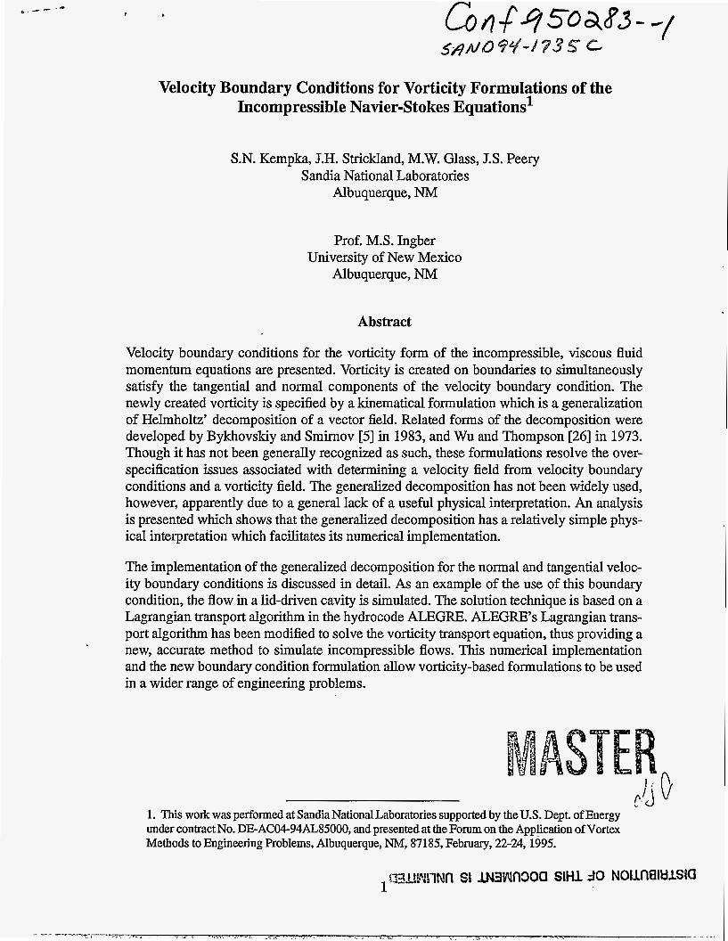
S+

Figure 2 Partitioning of a vortex sheet y (that satisfies the normal velocity boundary condition) into two shEets, y and yc. ybc lies outside the fluid, and represents the tangential-b$elocity boundary condition,

= -2 x z&. yc lies in the fluid, representing vorticity created in the fluid, and has stfength y = y-y . The tangential velocity boundary condition is satisfied on i%e i n k f i & between the two sheets. ' b G

The unknown y can be determined by writing the tangential component of Eq. (21) at discrete 1ocations"on the boundary and solving the resulting set of linear equations. The tangential velocity on S- is 6 x y which is not generally the specified tangential velocity boundary condition? The vortex sheet y, however, contains the "boundary condition vortex sheet" ybc = -6 x ub , with the exce"s vortex sheet strength y = y- 'ybc representing the vorticity that is created in the fluid.

"C "

From another point of view, the tangential velocity boundary condition is used to partition y into two vortex sheets: one which remains outside the fluid, T ~ ~ , and the other which en- Grs the fluid (representing vorticity created in the fluid y = y- y ). Figure 2 shows the configuration of the two sheets. It can be shown that the-&gential velocity boundary condition is satisfied on the interface between the two sheets. Substituting y = ybc + yc and

= -2 x g b into Eq. (21) yields the initial statement of the generalized theorem, Eq. ($. The tangential velocity boundary condition therefore specifies how y is to be parti- tioned, thus specifying how much vorticity is created in the fluid. This shows that there is no over-specification of vorticity creation.

- -bc

Y C

This formulation provides a mathematical basis for the approach suggested by Lighthill [lS]. As discussed in the introduction, in Lighthill's approach, the additive potential velocity field results in a deviation from the tangential velocity boundary condition, or "slip"

3. Although only the tangential component of was Eq. (21) solved, the normal velocity boundary condition is enforced since g,, = 0, as discussed in item 3 of the previous section.

13

velocity, uslip. The slip velocity is taken to represent a vortex sheet with a strength equal to the opposite of the slip velocity.

The generalized decomposition shows explicitly how this is true. In the generalized decomposition, the normal velocity boundary condition can be satisfied only if a vortex sheet y exists on the boundary, with y = -2 x uszip?. Eq. (14) (with us, = 0 ) shows that the v&ex sheet at a particular bound“ary location eliminates only half of the slip, and the other half is eliminated by the motion induced by the other vortex sheets and the previously existing vorticity.

Finally, it is noted that the boundary integrals in the generalized decomposition are not merely a representation of a traditional potential velocity field V@ . Consider that V@ is constrained by IV@ 0QdS = 0, whereas uszip is constrained more generally by IgdV = Jfi x u,,,tdS, which simplifies to the traditional constraint for potential flows J i ix us,,tdS = 0 if g = 0.

Fractional Step Numerical Formulation

1. General Solution Procedure A numerical scheme to solve the incompressible Navier-Stokes equations is developed. The vorticity form of the Navier-Stokes equations for a constant density and constant viscosity fluid is

%+ (zJ.V)g = (cpV)zJ+vV2c$ at

in the domain R. (22)

Eq. (22) describes simultaneously inviscid transport and viscous transport, and could be solved using finite or finite difference methods. However, inviscid transport can be greatly simplified using a lagrangian interpretation, so inviscid transport and viscous transport are considered sequentially. Inviscid transport is described by

%+ (zJ.V)(j) = (g.V)zJ at which, according to Helmholtz’ theorem, is also described by moving particles of vorticity at the local fluid velocity, which is described by,

where x (a, t=O) = a is the starting point of a particle.

This is the basis for Lagrangian vortex blob methods, and is closely related to the basis by which momentum transport is described in many shock wave physics or “hydrocodes”

14

used to model high pressure (mega-bars), high velocity (km/s) compressible phenomena. See Benson [3]. Hydrocodes describe momentum transport by solving,

wherein Eq. (25) describes the motion of points on discrete volumes, which contain quan- tities to be transported, such as mass and energy.

To describe incompressible flows, the algorithm used in hydrocodes has been adapted to solve Eq. (24) to describe vorticity transport. Two other investigations are also in progress regarding this approach, and have had encouraging results. See Bless and Chacon [4], and Russo and Strain [24].

Diffusion of vorticity into the domain and diffusion of vorticity within the domain are described by solving

with the boundary condition

z v(fi.Vm,) = - At *

In the domain, the velocity field in the domain is obtained from the vorticity field and the velocity boundary conditions using Eq. (5).

To briefly summarize the algorithm, first, the vortex sheet is determined which satisfies the normal velocity boundary condition. Second, the vortex sheet is moved to lie inside the fluid, such that the tangential velocity boundary condition is also satisfied. (This step requires no effort--it’s purely conceptual.) Third, the vorticity field is transported inviscidly. Fourth, viscous diffusion of the vorticity field is described, including the flux of vorticity from the boundaries. At this point, the velocity boundary conditions are no longer satisfied, so that new vortex sheets must be found on the boundary, which begins the repetition of the algorithm.

Example of the Algorithm: Impulsively Started, Driven Lid Cavity

The incompressible flowfield in a two-dimensional cavity with a moving lid is simulated to demonstrate the introduction of vorticity into fluid using the generalized decomposition. This is intended to be a demonstration, rather than a validation, of the proposed algorithm, although the results presented fall within the ranges of previously reported solutions for a Reynolds number of unity. A validation of the algorithm would require

15

Moving Lid B. C. on fluid: ut = -1, q, = 0

Figure 3 Schematic of a driven-lid cavity. The top of the cavity moves from left to right, imparting motion to the fluid via the no-slip boundary condition. The tangential velocity on all other boundaries is zero. In addition, the normal velocity is zero on all boundaries.

comparisons of solutions over a wide range of Reynolds numbers, which has not been completed at this time. This demonstration merely shows the algorithmic process by which vorticity is introduced into the fluid. The Lagrangian transport algorithm in the hydrocode ALEGRE was modified to perform this simulation. Steady-state results were obtained by solving the transient equations until steady-state was reached.

For this preliminary calculation, constant, discontinuous boundary elements were used to represent the boundary integrals, with a single point collocation scheme for evaluating the vortex sheet strengths. For this simple representation, the velocity boundary conditions are satisfied only on average on an element, and the integrals constraints are satisfied only to within a few percent. As discussed below, however, this simple scheme yields accurate results. Thus, we view this simple and not very accurate scheme as a preliminary numerical validation of the generalized decomposition, and are presently developing more accurate schemes, including a Galerkin weighted residual method.

The major feature of the flow field in a lid-driven cavity is the recirculation motion shown in Figure 3. (Smaller recirculation regions, or Moffatt eddies [16] occur in the corners.) This problem has been used as a test of the ability of Navier-Stokes codes to resolve recirculating motion (see Olson [2O],Winters and Cliffe [25], and Ghia, et al. [SI. A principal quantitative diagnostic is the location of the center of the largest recirculation region xv = (xv, yv) . For a Reynolds number of unity, in a square of unit width and height, the center of the recirculation region lies at xv = 0.5 , and 0.794 2 yv 2 0.75 for discretiza- tions ranging from 10 X 10 to 101 X 101, with no apparent dependence on discretization, for a number of analyses, as summarized by Olson [20]. Using the proposed vorticity for-

16

0,o -x

Figure 4 Velocity vectors and vorticity contours for a lid-driven cavity, fora Reynolds number of unity. The cavity is square, each side has unit length, the lid motion is left to right, the grid is 10 X 10, and the center of the primary vortex is xv = (0.5,0.754), which is within the range of previously reported results

mulation with a 10 X 10 grid, the vortex center obtained is xv = (0.5,0.754), which is in the range of previously reported results. Velocity vectors and lines of constant vorticity are shown in Figure 4.

Summary

A generalization of Helmholtz' decomposition is used to formulate velocity boundary conditions for vorticity forms of the incompressible Navier-Stokes equations. The generalized decomposition shows that velocity boundary conditions ub can be represented as vortex sheets and sources sheets on the boundary. The strengths of the sheets are -6 x gb and -6 e z& for vortex sheets and source sheets, respectively. This representation yields zero velocity outside the sheets, for which it was shown that satisfaction of one component of the velocity boundary condition implies the satisfaction of all components of the velocity boundary condition. Thus, a single (normal or tangential) component of the boundary velocity vector is sufficient to determine the vorticity generated in the fluid that satisfies the velocity boundary conditions.

The generalized decomposition provides the basis for a no-slip boundary condition in which velocity boundary conditions are satisfied by the creation of vorticity in fluid, adja-

17

cent to the boundary. The unknown vorticity is determined from in the form of a vortex sheet, from which a diffusive flux of vorticity into the fluid is determined.

A preliminary calculation using a modified hydrocode ALEGRE was also presented. The use of ALEGRE’s Lagrangian step and remap capability to solve the inviscid transport equation for vorticity provides a highly accurate formulation to describe incompressible transient flows.

References

1

2

3

4

5

6

7

8

9

10

11

Anderson, C. R., “Vorticity Boundary Conditions and Boundary Vorticity Genera- tion for Two-Dimensional viscous Incompressible Flow,” Journal of Computational Physics, vol. 80, pp. 72-97, 1989.

Batchelor, G. K., An Introduction to Fluid Mechanics, Cambridge University Press, 1967.

Benson, D. J., “Computational Methods in Lagrangian and Eulerian Hydrocodes,” In Computer Methods in Applied Mechanics and Engineering, vol. 99, pp. 235-394, 1992.

Bless, I. and T. Chacon, “Some Performing 2D Vortex Methods with Finite Ele- ments,” Finite Elements in Fluid, K. Morgan, E. Onate, J. Periauz, J. Peraire, and O.C. Zienkeiwicz, Eds., CIMNlYPinerigde Press, 1993.

Bykhovskiy, E. B. and N. V. Smirnov, “On Orthogonal Expansions of the Space of Vector Functions which are Square-Summable over a Given Domain and the Vector Analysis Operators,” NASA TM-77051, 1983.

Chorin, A. J. and J. E. Marsden, A Mathematical Introduction to Fluid Mechanics, Second Edition, Springer-Verlag, 1990

Gresho, P. M., “Incompressible Fluid Dynamics: Some Fundamental Formulation Is- sues,’, Ann. Rev. Fluid Mech., vol. 23, pp. 413-453, 1991.

Ghia, U., Ghia, K.N., and C.T. Shin, “High-Re Solutions for Incompressible Flow Using the Navier-Stokes Equations and a Multigrid Method,” Journal of Computa- tional Physics, Vol. 28, pp. 387-411, 1982.

Hung, S. C., and R.B. Kinney, “Unsteady Viscous flow over a Grooved Wall: A Comparison of two Numerical Methods, Int. J. Numer. Methods Fluids, vol. 8, pp. 1403-1437,1988.

Kellog, 0. D, Foundations of Potential Theory Dover, 1953.

Kinney, R. B., and M.A. Paolino, ASME J. Appl. Mech., ~0141,1974

18

12 Kinney, R. B., and 2. M. Ceilak, AIAA J., vol. 15, no. 12, p. 1712,1977.

13 Korn, G. A. and T. M. Korn, Mathematical Handbook for Scientists and Encineers, McGraw-Hill, 2nd Edition, 1968

14 Koumoutsakos, P., Leonard, A., and E Pepin, “Boundary Conditions for Viscous Vortex Methods,” Journal of Computational Physics, vol. 113, pp. 52-61,1994.

15 Lighthill, M. J., “Chapter II. Introduction: Boundary Layer Theory,” in Laminar Boundary Layers, Rosenhead, L., Editor, Oxford at the Clarendon Press, 1963.

16 Moffatt, H. K., “Viicous and Resistive Eddies Near a Sharp Corner,” J. Fluid Mech., VOI. 79, pp. 391-414, 1964

17 Morino, L., “Helmholtz Decomposition Revisited: Vorticity Generation and Trailing Edge Condition,” Computational Mechanics, vol. 1, pp. 65-90,1986.

18 Morino, L., “Boundary Integral Equations in Aerodynamics,” Applied Mechanics Reviews, vol. 46, no. 8, pp. 445,-466, August 1993.

19 Morton, B. R., “The Generation and Decay of Vorticity,’, Geophys. Astrophys. Fluid Dyn., vol. 1, pp. 65-90, 1984.

20 Olson, M.D., “Comparison Problem No. 1: Recirculating Flow in a Square Cavity,’, Structural Research Series Report No. 22, I.S.S.N. 0318-3378, The University of British Columbia Dept. of Civil Engineering, May, 1979.

21 Puckett, E. G., “Vortex Methods: An Introduction and Survey of Selected =search Topics,” in Incompressible Computational Fluid Dvnamics, edited by M.D. Gun- zburger and R. A. Nicolaides, Cambridge University Press, 1993.

22 Quartapelle, L., “Vorticity Conditioning in the Computation of Two-dimensional Viscous Flows, J. Comput. Phys., vol. 40, pp. 453-477,1981.

23 Quartapelle, L. and F. Valz-Gris, “Projection Conditions on the Vorticity in Viscous Incompressible F~ows,’~ International Journal for Numerical Methods in Fluids, vol. 1, pp. 129-144, 1981.

24 Russo, G. and J. A. Strain, “Fast Triangulated Vortex Methods for the 2D Euler Equations,” J. Comput. Phys., vol. 111, pp. 291-323,1994.

25 Winters, K. H., and K.A. Cliffe, “A Finite Element Study of Driver Laminar Flow in A Square Cavity,’, United Kingdom Atomic Energy Authority, Harwell Oxfordshire, AERE-R 9444,1979.

26 Wu, J. C. and J. F. Thompson, “Numerical Solutions of Time-Dependent Incom- pressible Navier-Stokes Equations Using an Integro-Differential Formulation,” Computers & Fluids, vol. 1, pp. 197-215, 1973.

19

- . .

27 Wu, J. C., “Numerical Boundary Conditions for Viscous Flow Problems,” AIAA Journal, vol. 14, pp. 1042-1047,1976.

28 Wu, J. C. and U. Gulcat, “Separate Treatment of Attached and Detached Flow Re- gions in General Viscous Flows,” AIAA Journal, vol. 19, no. 1, pp. 20-27,1981.

29 Wu, J. C., “Boundary Elements and Viscous Flows,” pp. 3-18, Boundary Element Technologv VII, Computational Mechanics Publications, co-published with Elsevier Applied Science, 1992, Edited by C. A. Brebbia and M. S . Ingber.

30 Wu, J., Wu X., Ma, H., and J. Wu, “Dynamic Voiticity Condition: Theoretical Anal- ysis and Numerical Implementation,” International Journal for Numerical Methods in Fluids, vol. 19, pp. 905-938, 1994.

DISCLAIMER

This report was prepared as an account of work sponsored by an agency of the United States Government. Neither the United States Government nor any agency thereof. nor any of their employees, makes any warranty, express or implied, or assumes any legal liability or responsi- bility for the accuracy, completeness, or usefulness of any information, apparatus, product, or process disclosed. or represents that its use would not infringe privately owned rights. Refer- ence herein to any specific commercial product, process, or service by trade name, trademark, manufacturer, or otherwise does not necessarily constitute or imply its endorsement, recom- mendation. or favoring by the United States Government or any agency thereof. The views and opinions of authors expressed herein do not necessarily state or reflect those of the United States Government or any agency thereof.

20

velocity boundary conditions for vorticity formulations …/67531/metadc681377/m2/1/high... ·...

Documents