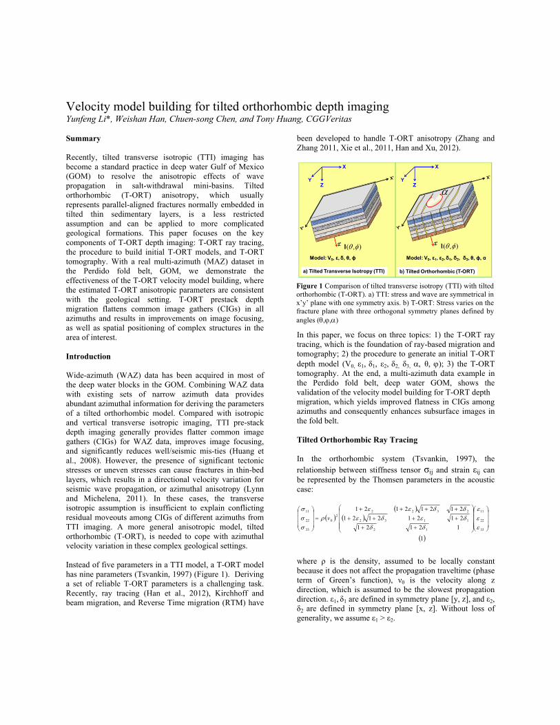
Velocity model building for tilted orthorhombic depth imaging Yunfeng Li*, Weishan Han, Chuen-song Chen, and Tony Huang, CGGVeritas Summary Recently, tilted transverse isotropic (TTI) imaging has become a standard practice in deep water Gulf of Mexico (GOM) to resolve the anisotropic effects of wave propagation in salt-withdrawal mini-basins. Tilted orthorhombic (T-ORT) anisotropy, which usually represents parallel-aligned fractures normally embedded in tilted thin sedimentary layers, is a less restricted assumption and can be applied to more complicated geological formations. This paper focuses on the key components of T-ORT depth imaging: T-ORT ray tracing, the procedure to build initial T-ORT models, and T-ORT tomography. With a real multi-azimuth (MAZ) dataset in the Perdido fold belt, GOM, we demonstrate the effectiveness of the T-ORT velocity model building, where the estimated T-ORT anisotropic parameters are consistent with the geological setting. T-ORT prestack depth migration flattens common image gathers (CIGs) in all azimuths and results in improvements on image focusing, as well as spatial positioning of complex structures in the area of interest. Introduction Wide-azimuth (WAZ) data has been acquired in most of the deep water blocks in the GOM. Combining WAZ data with existing sets of narrow azimuth data provides abundant azimuthal information for deriving the parameters of a tilted orthorhombic model. Compared with isotropic and vertical transverse isotropic imaging, TTI pre-stack depth imaging generally provides flatter common image gathers (CIGs) for WAZ data, improves image focusing, and significantly reduces well/seismic mis-ties (Huang et al., 2008). However, the presence of significant tectonic stresses or uneven stresses can cause fractures in thin-bed layers, which results in a directional velocity variation for seismic wave propagation, or azimuthal anisotropy (Lynn and Michelena, 2011). In these cases, the transverse isotropic assumption is insufficient to explain conflicting residual moveouts among CIGs of different azimuths from TTI imaging. A more general anisotropic model, tilted orthorhombic (T-ORT), is needed to cope with azimuthal velocity variation in these complex geological settings. Instead of five parameters in a TTI model, a T-ORT model has nine parameters (Tsvankin, 1997) (Figure 1). Deriving a set of reliable T-ORT parameters is a challenging task. Recently, ray tracing (Han et al., 2012), Kirchhoff and beam migration, and Reverse Time migration (RTM) have

been developed to handle T-ORT anisotropy (Zhang and Zhang 2011, Xie et al., 2011, Han and Xu, 2012).

In this paper, we focus on three topics: 1) the T-ORT ray tracing, which is the foundation of ray-based migration and tomography; 2) the procedure to generate an initial T-ORT depth model (V0, ε1, δ1, ε2, δ2, δ3, θ, ; 3) the T-ORT tomography. At the end, a multi-azimuth data example in the Perdido fold belt, deep water GOM, shows the validation of the velocity model building for T-ORT depth migration, which yields improved flatness in CIGs among azimuths and consequently enhances subsurface images in the fold belt. Tilted Orthorhombic Ray Tracing In the orthorhombic system (Tsvankin, 1997), the relationship between stiffness tensor σij and strain εij can be represented by the Thomsen parameters in the acoustic case:

1

12121

21212121

21212121

33

22

11

12

1132

23222

0

33

22

11

v

where ρ is the density, assumed to be locally constant because it does not affect the propagation traveltime (phase term of Green’s function), ν0 is the velocity along z direction, which is assumed to be the slowest propagation direction. ε1, δ1 are defined in symmetry plane [y, z], and ε2, δ2 are defined in symmetry plane [x, z]. Without loss of generality, we assume ε1 > ε2.

Figure 1 Comparison of tilted transverse isotropy (TTI) with tiltedorthorhombic (T-ORT). a) TTI: stress and wave are symmetrical inx’y’ plane with one symmetry axis. b) T-ORT: Stress varies on thefracture plane with three orthogonal symmetry planes defined byangles (,,)

Velocity model building for tilted orthorhombic depth migration

Following the quasi acoustic approximation (Han and Xu, 2012), the Hamilton equation is represented as

22

112

22

221

22

2222

2

)(2

;2121

:

2244

1

))()((2

1),(

zyx

zyx

yx

p

pppL

pppK

where

sppAEBALKK

xsppxH

(7)

where λp is the eigenvalue of orthorhombic characteristic matrix for P wave and ),,( zyx ppppp

is the slowness

vector, which is specified in point ),,( zyxxx in ray

direction n

, np p

2/1 .

Orthorhombic kinematic raytracing equations system can be established by integrating this Hamiltonian system:

3

/),(

/2),(

/2),(

/2),(

2222

222

222

222

d

dzp

d

dyp

d

dxp

d

dT

MUppNpRsssdx

pxdH

d

pd

MpFpGpsdp

pxdH

d

dz

MppBEABFpAsdp

pxdH

d

dy

MppBEABGpBsdp

pxdH

d

dx

zyx

yxz

zyxz

yxzy

xyzx

where x is a function of τ, xx

BEBAU

FpGpNppRKsM

EDCBA

yxyx

3212

22

1

2

2

22

32121

2

,,,2

,21,21,21,21,21

In tilted orthorhombic media, the transformation system between the physical coordinates and the rotated coordinates can be defined as the equation (4), where all three symmetry axes are aligned with coordinate axes:

4

100

0cossin

0sincos

cos0sin

010

sin0cos

100

0cossin

0sincos

'

'

'

z

y

x

z

y

x

As in conventional TTI, θ and φ are defined by the rotation of the vertical axis at each spatial location. is the rotation angle of the elastic tensor in [x’, y’] plane, which is identical to the angle between the crack orientation and the (arbitrarily chosen) y’ axis. (x, y, z) are the spatial coordinates in physical coordinates and )',','( zyx are the

coordinates of the same point in the rotated system, which now has the orthorhombic symmetry planes aligned with the coordinate axes.

Estimation of Initial Tilted Orthorhombic Model

The derived T-ORT ray tracing (Equation 3) is applied to obtain traveltimes for prestack Kirchhoff or Beam depth migration, which also provide necessary tools for T-ORT tomography. There are nine inter-dependent parameters to be determined for the T-ORT model, of which V0, ε1, ε2 and are the most sensitive to T-ORT ray tracing. Here, we describe how we initialize the T-ORT model. We start from conventional TTI model building.

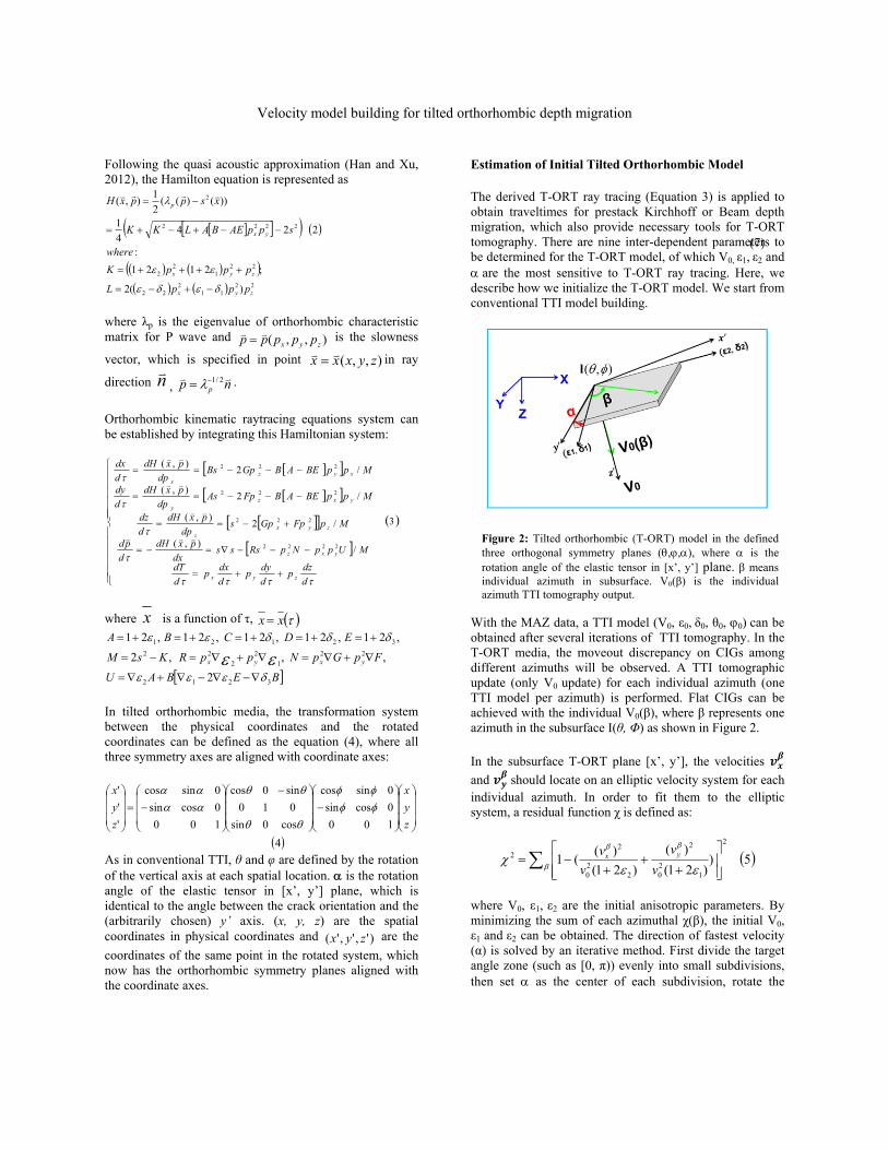
With the MAZ data, a TTI model (V0, ε0, δ0, θ0, 0can be obtained after several iterations of TTI tomography. In the T-ORT media, the moveout discrepancy on CIGs among different azimuths will be observed. A TTI tomographic update (only V0 update) for each individual azimuth (one TTI model per azimuth) is performed. Flat CIGs can be achieved with the individual V0(β), where β represents one azimuth in the subsurface I(θ, Φ) as shown in Figure 2.

In the subsurface T-ORT plane [x’, y’], the velocities

and should locate on an elliptic velocity system for each individual azimuth. In order to fit them to the elliptic system, a residual function χ is defined as:

5))21(

)(

)21(

)((1

2

120

2

220

22

v

v

v

v yx

where V0, ε1, ε2 are the initial anisotropic parameters. By minimizing the sum of each azimuthal χ(β), the initial V0, ε1 and ε2 can be obtained. The direction of fastest velocity (α) is solved by an iterative method. First divide the target angle zone (such as [0, π)) evenly into small subdivisions, then set as the center of each subdivision, rotate the

Figure 2: Tilted orthorhombic (T-ORT) model in the defined three orthogonal symmetry planes (,,), where is the rotation angle of the elastic tensor in [x’, y’] plane. β means individual azimuth in subsurface. V0(β) is the individual azimuth TTI tomography output.

Velocity model building for tilted orthorhombic depth migration

system by , calculate the residual χ, and then choose the smallest one to be the target angle zone for the next iteration. After the length of the target angle zone is small enough, we obtain the initial α as well as V0, ε1 and ε2. At least three azimuths of data are needed for estimation of initial T-ORT model. With the same elliptic fitting method used to derive ε1 and

ε2, δ1 and δ2 are obtained. δ3 can be derived by the acoustic approximation in the orthorhombic system (Tsvankin, 1997) and (θ, are inherited from the TTI model. At this stage, we have obtained initial models for the nine T-ORT attributes (V0, ε1, δ1, ε2, δ2, δ3, θ, . Tilted Orthorhombic Tomography By the implementation of the orthorhombic ray tracing in Equation (3), the T-ORT migration is performed with the initial models to generate MAZ CIGs, based on which the residual curvatures are picked. In orthorhombic media, slowness in direction , , can be calculated using the formula

6)))((4/(2 22222yxn

nnAEBALKKss

where is a unit vector in the target direction; A, B, E, K, and L are defined as before (Equation 3). Similarly to the method used in VTI and TTI tomography, we set up a sparse linear system based on the invariant of travel time:

∆→∆

→∆

→∆

(7) Here ∆ is the difference between the picked event depth and the true depth, and is the length of the ray in each cell of the velocity model. T-ORT model updates (V0 only;

ε1,ε2; or V0 , ε1, ε2, ) are obtained by solving this linear system. If there is any well information available, this information, such as mis-tie, can be incorporated to constrain the T-ORT tomographic output.

Application We apply the T-ORT model building methodology to an area in the Perdido fold belt in the northwestern GOM. The fold belt consists of a series of folds bounded by steep reverse faults. Factures in the fold belt are likely a natural cause of orthorhombic anisotropy. The input data consist of one wide-azimuth survey and one orthogonal narrow-azimuth survey, which give four azimuth sectors (0 o, 30o,

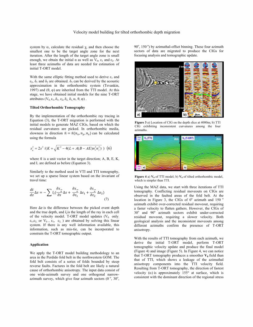
90o, 150 o) by azimuthal-offset binning. These four azimuth sectors of data are migrated to produce the CIGs for focusing analysis and tomographic update.

Using the MAZ data, we start with three iterations of TTI tomography. Conflicting residual moveouts on CIGs are observed in the faulted areas of the fold belt. At the location in Figure 3, the CIGs of 0o azimuth and 150 o azimuth exhibit over-corrected residual moveout, requiring a faster velocity to flatten gathers. However, the CIGs of 30o and 90o azimuth sectors exhibit under-corrected residual moveout, requiring a slower velocity. Both geological analysis and the inconsistent moveouts among different azimuths confirm the presence of T-ORT anisotropy. With the results of TTI tomography from each azimuth, we derive the initial T-ORT model, perform T-ORT tomographic velocity update and produce the final model (Figure 4) and image (Figure 5). In Figure 4, we can notice that T-ORT tomography produces a smoother V0 field than that of TTI, which shows a leakage of the azimuthal anisotropy components into the TTI velocity field. Resulting from T-ORT tomography, the direction of fastest velocity (is approximately 155° at surface, which is consistent with the dominant direction of the regional stress

Figure 3 a) Location of CIG on the depth slice at 4000m; b) TTI CIG exhibiting inconsistent curvatures among the four azimuths.

0o

Figure 4 a) V0 of TTI model; b) V0 of tilted orthorhombic model, which is simpler than TTI.

Velocity model building for tilted orthorhombic depth migration

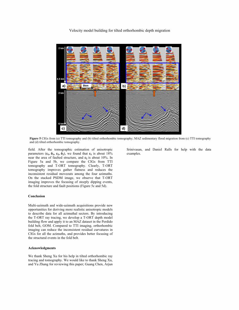
field. After the tomographic estimation of anisotropic parameters (ε1, δ1, ε2, δ2), we found that ε1 is about 18% near the area of faulted structure, and ε2 is about 10%. In Figure 5a and 5b, we compare the CIGs from TTI tomography and T-ORT tomography. Clearly, T-ORT tomography improves gather flatness and reduces the inconsistent residual moveouts among the four azimuths. On the stacked PSDM image, we observe that T-ORT imaging improves the focusing of steeply dipping events, the fold structure and fault positions (Figure 5c and 5d). Conclusion

Multi-azimuth and wide-azimuth acquisitions provide new opportunities for deriving more realistic anisotropic models to describe data for all azimuthal sectors. By introducing the T-ORT ray tracing, we develop a T-ORT depth model building flow and apply it to an MAZ dataset in the Perdido fold belt, GOM. Compared to TTI imaging, orthorhombic imaging can reduce the inconsistent residual curvatures in CIGs for all the azimuths, and provides better focusing of the structural events in the fold belt. Acknowledgments We thank Sheng Xu for his help in tilted orthorhombic ray tracing and tomography. We would like to thank Sheng Xu, and Yu Zhang for reviewing this paper; Guang Chen, Arjun

Srinivasan, and Daniel Ralls for help with the data examples.

Figure 5 CIGs from (a) TTI tomography and (b) tilted orthorhombic tomography; MAZ sedimentary flood migration from (c) TTI tomography and (d) tilted orthorhombic tomography.

Velocity model building for tilted orthorhombic depth migration

References

Han, W. and Xu, S., 2012, Orthorhombic raytracing and traveltime calculation, 74th Annual Internat. Mtg., Eur. Assn. Geosci. Eng. (accepted) Huang, T., Xu, S., Wang, J. and Ionescu, G. 2008, The benefit of TTI for dual-azimuth data in Gulf of Mexico, SEG Expanded Abstract, 27, 222-226 Lynn, H.B. and Michelena, R.J., 2011, Introduction to this special section: practical applications of anisotropy, The Leading Edge, 726-730. Tsvankin, I., 1997, Anisotropic parameters and P-wave velocity for orthorhombic media: Geophysics, 62, 1292-1309. Xie, Y., Birdus S., Sun J., Notfors C., 2012, Prestack depth imaging of multi-azimuth seismic data in the presence of orthorhombic anisotropy,22th Internat. Mtg., ASEG. Zhang, H. and Zhang, Y., 2011, Reverse Time Migration in Vertical and Tilted Orthorhombic Media, SEG Expanded Abstract, 30, 185-189.

Thomas, M. and Veronique, F., 2002, P-wave Tomography in Inhomogeneous Orthorhombic Media, Pure appl. Geophys. 159, 1855-1879.