Venture capital, entrepreneurship and economic growth∗

Sampsa Samila†

Faculty of Business

Brock University

Olav Sorenson‡

School of Management

Yale University

June 7, 2009

Abstract: Using a panel of US metropolitan areas from 1993 to 2002, we find that an

increase in the local supply of venture capital (VC) positively affects (i) the number of firm

starts, (ii) employment, and (iii) aggregate income. Our results remain robust to specifica-

tions that address potential endogeneity in the supply of venture capital by using endowment

returns as an instrumental variable. The magnitudes of the effects moreover imply that ven-

ture capital stimulates the creation of more firms than it directly funds. That result appears

consistent with either of two mechanisms: One, would-be entrepreneurs that anticipate a

future need for financing more likely start firms when the supply of capital expands. Two,

VC-funded companies may transfer tacit knowledge to their own employees enabling spinoffs,

and may encourage both their employees and others to become entrepreneurs through demon-

stration effects.

Keywords: Venture capital, financial intermediaries, entry, employment, wage bill

JEL Classification: G24, L26, O43, R11

∗Sorenson gratefully acknowledges financial support from the Social Science and Humanities ResearchCouncil of Canada (Grant # 410-2007-0920). We also thank Constanca Esteves-Sorenson, Tim Simcoe,Scott Stern, Will Strange and one anonymous reviewer for their helpful advice.

†500 Glenridge Ave, St. Catharines, ON L2S 3A1, Canada; sampsa.samila@brocku.ca‡135 Prospect St, P.O. Box 208200, New Haven, CT 06520-8200; olav.sorenson@rotman.utoronto.ca

1

1 Introduction

Analysts, bureaucrats, business leaders, politicians and pundits have widely pointed to ven-

ture capital (VC) as an important factor underlying the economic growth both of certain

regions within the United States, such as Silicon Valley, as well as of the country as a whole

(Bottazzi and Rin 2002). These commentators have similarly attributed slow growth to the

relative scarcity of venture capital in states from Alaska to Florida, and in nearly every coun-

try aside from the United States. Several governments, including those of Canada, Chile,

Germany and Israel, in the interest of stimulating their economies, have even sought to ex-

pand their local supplies of venture capital by way of public policy (Gilson 2003; Cumming

and MacIntosh 2007).

Despite the widespread interest in venture capital as a stimulus for economic growth, how-

ever, little empirical research has examined the validity of these claims (for an exception,

see Hasan and Wang 2006). At first blush, positive relationships between venture capital,

entrepreneurship and economic growth might appear a foregone conclusion, but these rela-

tionships, in fact, rest on two (potentially inaccurate) assumptions. First is a presumption

that VC-funded firms would not have come into being without venture capital, and second is

a belief that those employed at these VC-funded firms generate substantially more value for

the economy than they would have in other firms. Although firm-level studies have found

that VC-funded companies enjoy higher employment and sales growth rates than the aver-

age startup (Jain and Kini 1995; Engel and Keilbach 2007), one cannot easily extrapolate

from these firm-level relationships to the implications of venture capital for the economy as

a whole. It is quite possible, for example, that VC firms simply select the more promising

startups and substitute for other sources of financing that those ventures would have received

had venture capital not been available. The macro-level relationships between the supply of

2

venture capital, entrepreneurship and economic growth therefore remain open questions.

To determine whether the availability of venture capital stimulates the formation of

new firms, and in turn contributes positively to economic growth, we exploited both cross-

sectional and longitudinal variation in the supply of venture capital across and within

Metropolitan Statistical Areas (MSAs). We estimated the local effects of venture capital

activity – measured in terms of (i) the number of companies funded, (ii) the number of

investments made, and (iii) the aggregate dollars invested – on the number of new firms

established, and on employment and aggregate income. Since the supply of venture capital

itself may depend in part on the demand for it – that is, on the availability of high potential

businesses in which to invest – we also used endowment returns as an instrument to identify

the supply of venture capital. Our results remained robust to these specifications.

Our findings imply that venture capital stimulates startup activity. A doubling in the

supply of venture capital in a region results in the establishment of 0.49% to 2.6% more new

establishments on average (depending on how one measures the supply of venture capital).

For the average MSA, a doubling in investments means moving from having four firms

funded per year to having eight firms funded per year. Our estimates therefore imply that an

additional investment would stimulate the entry of 7 to 36.7 establishments—in other words,

more new firms than actually funded. A doubling in the supply of venture capital also results

in a 0% to 1.0% expansion in the number of jobs, and a 1.4% to 6.4% increase in aggregate

income. These results appear consistent with either of two potential mechanisms. First,

nascent entrepreneurs may recognize the need for capital in the future and only establish

firms when they perceive reasonable odds of obtaining that funding. Second, VC-funded

firms may encourage others to engage in entrepreneurship either through a demonstration

effect or by training future firm founders.

3

By providing evidence that the supply of venture capital positively stimulates entrepreneur-

ship and aggregate regional income, our findings contribute to the literature that has been

attempting to explain cross-regional differences in economic outcomes (e.g., Glaeser et al.

1992; Rosenthal and Strange 2003). Whereas the existing literature has focused primarily

on agglomeration externalities, either within or across industries, however, our results – sim-

ilar to many cross-national studies of economic growth (e.g., Rodrik et al. 2004) – suggest

that heterogeneity in economic institutions also contribute to regional differences in growth.

In particular, consistent with the theoretical literature, an expansion in the availability of

financial intermediaries, in this case venture capitalists, stimulates economic development

(Greenwood and Jovanovic 1990; Keuschnigg 2004). Dynamic regions, such as Silicon Val-

ley, have benefited not just from technological shocks and inter-firm spillovers, but also from

the fact that they have had the financial infrastructure necessary to help transform these

ideas into productive firms.

2 Venture capital and economic growth

Venture capital, the funding of high-potential companies through equity investments by

professional financial intermediaries, has existed in the United States for more than 60 years.

Despite some prominent early success stories, these intermediaries played only a minor role

in the financing of early-stage companies prior to the 1980s (Gompers and Lerner 1998).

Since then, however, their prominence has been rising rapidly; according to the National

Venture Capital Association (NCVA), from 1978 to 2007, the total funds raised by venture

capital firms in the United States grew from $549 million (in 2007 dollars) to $35.9 billion.

In the United States, venture capital firms have evolved toward a common organizational

form. Each firm consists of one or more limited partnerships, called funds, with lifespans of 10

4

to 12 years. The capital in these funds comes from passive limited partners, primarily wealthy

individuals and institutional investors, such as college endowments, insurance companies

and pension funds. The general partners, often referred to as venture capitalists, actively

manage this capital—identifying attractive investments and then monitoring and advising

the companies in which they invest to maximize their returns. In exchange for their services,

venture capitalists receive both some fixed compensation and a potentially sizable portion

of the capital gains earned on these investments. They therefore have strong incentives to

choose their portfolio companies wisely and to nurture them as effectively as possible.

Evidence from firm-level studies generally suggests that venture capitalists produce value

through their pre- and post-investment roles (i.e through the selection and advising of port-

folio companies). Jain and Kini (1995), for example, found that firms financed by venture

capital grew faster in sales and in employment. Analyses of the financial returns to ven-

ture capital investments paint a similar picture (Chen et al. 2002; Cochrane 2005). But the

interest in venture capital reflects not only its value to those investing in it, but also its

potential to contribute to the economy as a whole by promoting the development of high

growth companies that create jobs and generate wealth.

2.1 Selection and substitution

Although firm- and investment-level studies find evidence consistent with the idea that ven-

ture capital firms create value for their investors, at least two important issues arise in

attempting to move from these studies to the potential benefits of venture capital to the

economy as a whole: (1) Would these companies have received funding from other sources

in the absence of venture capital? (2) How much of the value of venture capital at the firm-

level stems from pre-investment activities (i.e. selection)? If these companies would have

5

found other sources of funding, then venture capitalists may do little more than help their

limited partners to find these investments (and, perhaps, to reduce slightly the cost of cap-

ital by intensifying competition in the financing of fledgling firms). Even if venture capital

firms do alleviate entrepreneurs’ capital constraints, firm- and investment-level studies could

overestimate the benefits of this capital to the economy as a whole if venture capitalists

cherry-pick the best investments. Venture capital may therefore have little or no net effect

on the economy as a whole.

Although research has not directly investigated the first issue, the literature on wealth

and entrepreneurship suggests that insufficient financial resources may prevent many from

starting their own businesses. Evans and Jovanovic (1989) and Blanchflower and Oswald

(1998), for example, have found that the odds of becoming an entrepreneur rise with house-

hold wealth. This relationship suggests that entrepreneurs cannot always find substitute

funds for good ideas. To the extent that access to financial resources forms a binding con-

straint on the ability of individuals to engage in entrepreneurship, one might then expect

venture capital – as well as other institutions that alleviate these constraints – to stimulate

growth by ensuring that good ideas receive funding (Keuschnigg 2004).

With respect to the second issue – the degree to which venture capitalists add value

through their pre-investment activities – at least two recent studies suggest that selection

accounts for a substantial portion of the returns to venture capital investing. In a sample

of German companies, Engel and Keilbach (2007) found that, companies receiving venture

capital had more patents at the time of funding than the average startup. But once they

controlled for this difference (through matching), these companies proved no more innovative

after receiving VC funding. Using a structural model to identify pre- versus post-investment

processes, Sorensen (2007) has estimated that roughly two-thirds of the variation across

6

venture capital firms in the probability that their portfolio companies would go public stems

from pre-investment sorting processes (i.e. selection). Hence, even if venture capital does

alleviate capital constraints, selection could still lead extrapolations from firm-level studies

to overestimate the effect of venture capital on the economy.

2.2 Expectations and spinoffs

Two other factors, expectations and spinoffs, however, suggest that venture capital may en-

courage the founding of even more companies than it funds directly. Firm- and investment-

level studies therefore could also understate the economic value of venture capital. Let us

consider expectations first. If entrepreneurs assess their odds of success before attempting

entry, then the availability of venture capital should positively affect the evaluations of a num-

ber of these would-be entrepreneurs. Without capital infusions, many capital-constrained

entrepreneurs would find it impossible to develop their businesses. Their anticipated odds of

success therefore depend on their expectations of gaining venture capital funding.1 Though

one might expect entrepreneurs to secure this funding prior to entry – thereby limiting the

effects of venture capital to the companies it actually funds – entrepreneurs often enter

first and pursue financing later for two reasons.2 One, beginning operations before pursu-

ing financing allows the founder to retain a larger share of the equity. The entrepreneur

therefore has a financial incentive to found the firm – if possible – before receiving funding.

Two, because of the information asymmetries inherent between entrepreneurs and investors,

many venture capital firms avoid investing in companies that have not already achieved

1Even in the absence of capital constraints, entrepreneurs might value the advice and connections thatventure capitalists can provide to their portfolio companies and therefore still see value in these financingrelationships.

2Consistent with this expectation, the median company in our data does not receive its first round ofventure capital investment until 1.6 years after being established.

7

rudimentary milestones—perhaps filing for a patent or creating a prototype of a product.

A second mechanism through which venture capital may engender entrepreneurship is

through spinoffs—that is, through one or more employee(s) in some incumbent firm starting

their own company. Venture capital can encourage spinoffs in at least two ways. The first is

a demonstration effect. When interviewed, entrepreneurs often say that they first thought of

starting a company when they saw someone else do it, potentially even in a different industry

(Sorenson and Audia 2000). Seeing others engage in entrepreneurship can encourage other

would-be entrepreneurs to start firms. The second is a training effect. Small, entrepreneurial

firms operate differently from larger, more bureaucratic organizations. Prior experience in

small (VC-backed) companies allows would-be entrepreneurs to absorb tacit knowledge on

how to design and manage effective entrepreneurial ventures.

Because both the expectations and spinoffs mechanisms imply effects external to the

companies that actually receive venture capital funding, their influence would not appear in

firm- or investment-level studies. We must move to a more macro level of analysis. Research

at that level has been more scarce. Some evidence exists for a positive relationship between

venture capital and patenting (Kortum and Lerner 2000; Hasan and Wang 2006), though

those results may reflect compositional differences in which industries attract venture capital

(Gans and Stern 2003). Venture capital activity also correlates positively with regional

GDP growth (Hasan and Wang 2006), though high growth regions might attract venture

capital. Our understanding of these relationships nonetheless remains limited. We therefore

investigated the degree to which venture capital stimulates the production of new firms, jobs

and income growth.

8

3 Empirical evidence

To assess these issues, we constructed an unbalanced panel covering all 329 Metropolitan

Statistical Areas (MSAs) in the United States from 1993 to 2002. Our data comprise infor-

mation from a variety of publicly available and proprietary sources. The data on regional

economic activity came from the Office of Advocacy of the Small Business Administration

(SBA), which reports information collected by the Census Bureau.3 Our information on

venture capital has been derived from Thomson Reuters’ VentureXpert database, and our

measures of endowment returns came from The Chronicle of Higher Education.

We chose MSAs as our geographic unit of analysis because they offered the finest-grained

regions that one might reasonably consider independent with respect to economic activity.

The U.S. Office of Management and Budget (OMB) defines each MSA in terms of a core

urban area, of at least 50,000 inhabitants. It also includes in each MSA any surrounding

counties with a high degree of social and economic integration with the urban core.4 In prac-

tice, the OMB assesses social and economic integration by observing commuting patterns. If

more than 25% of a county’s residents commute to the urban core for work, then the OMB

includes the county in the MSA. Because a few regions only became classified as MSAs after

1993, our panel includes a total of 3,280 MSA-years.

We limited our analyses to a ten-year window, from 1993 to 2002, because the construc-

tion of the panel requires consistent definitions of the regional units of analysis across years.

Roughly three years after each decennial census, the OMB redefines the statistical areas for

3The Census Bureau polls the country each March. The firm birth data, therefore, count the numberof new firms from the beginning of April of a given year to the end of March in the next year. We haveused the exact dates of investments from the venture capital data to align the timing of investments to theCensus Bureau calendar.

4In contrast to the rest of the country, the Census Bureau uses townships, instead of counties, in NewEngland to determine the boundaries of MSAs.

9

the next ten years on the basis of the decennial data. The 1993 redefinition governed the

reporting of most government statistics from 1993 to 2002. Developing consistent regions

across these redefinitions would require a host of assumptions regarding the distribution of

activity within each MSA.

3.1 Cross-sectional estimates

We began our analysis by estimating effects from cross-sectional variation across MSAs.

In particular, we examined the effects of venture capital on three different outcomes: the

number of establishments in the region, overall employment in the region, and aggregate

income for the region.5 Our measure of employment includes both full-time employees and

(the full-time equivalent of) part-time employees. Aggregate income includes all forms of

compensation: wages, salary, bonuses and benefits. For each of these outcomes, we estimated

the effects using the following partial linear adjustment model:

ln Yi,t2 = β1 ln Fi,t1 + β2 ln Ei,t1 + β3 ln Wi,t1 + β4 lnt1−1∑

s=t1−5

Ii,s + β5 lnt1−1∑

s=t1−5

V Ci,s + εi, (1)

where i indexes the MSA observed at two points in time, t1 and t2. Yi,t2 denotes the

dependent variable (i.e. establishments, employment, and total payroll). Fi,t1, Ei,t1 and

Wi,t1 are the number of firms, employees, and the aggregate wages in the region respectively.

In each model, one of these measures serves as a lagged dependent variable. Ii,t1 controls

for innovation in the region (through patent counts); V Ci,t measures the supply of venture

5Alternatively, one might focus only on those establishments started in the industries most relevant toventure capital. Restricting the range of industries included would nevertheless have two disadvantages.From a practical point of view, venture capital firms have invested in nearly every 2-digit SIC code, so wewould have little ability to discriminate across industries in their potential for receiving venture capital. Butalso, from a theoretical perspective, to the extent that venture capital stimulates the founding and growth ofcompanies not directly funded by it, excluding some industries from the analyses would result in downwardbias in the effects of venture capital on the economy.

10

capital, and εi represents a normally distributed error term.

The opportunities to create firms and to invest in venture capital might both depend on

the arrival of new technological opportunities (Ii,t1). To control for these opportunities, we

used the count of patent applications (eventually approved) made by inventors located in an

MSA over the preceding five years. If a patent application had multiple inventors listed (n),

we assigned 1/n patents to the MSA of each inventor.

As a measure of venture capital activity, we counted the number of firms funded over

the preceding five years by VC firms located in a particular MSA. Because some regions

have no activity, we added one to this count before logging it. To focus on the number of

companies funded, we counted only initial investments in target companies (other measures

are examined below).6 We included all target companies in this count regardless of whether

those companies resided in the same MSA as the VC firm.7 So, for example, if a San Diego

target company received three rounds of capital infusions from a venture capital firm located

in Orange Country, we would increment this measure by one in Orange County in the year

of the first investment. Although VC firms tend to invest in close proximity to their offices

and therefore in firms located in the same MSA (Sorenson and Stuart 2001), they sometimes

do invest further away.

In counting venture capital investments, we restricted the VentureXpert data to limited

partnerships with a stated focus on seed stage, early stage, later stage, expansion, devel-

opment, or balanced stage investing.8 The VentureXpert database includes information on

6In cases that involved multiple VC firms investing in a single target, we counted each VC firm as havingmade one investment.

7Alternatively, one might locate investments according to the headquarters of the companies funded(rather than by the location of the VC firms). We dismissed this alternative because the logic of ourinstrumental variable allows us to identify the local supply of venture capital (rather than its deployment).To the extent that VC firms invest outside of their MSAs, however, our estimates should err on the side ofbeing conservative.

8An examination of the actual investments made by these funds confirmed that venture capital firms

11

many private equity partnerships that do not invest in early stage companies, such as LBO,

real estate and distressed debt funds, and funds of funds. The fund focus information allowed

us to remove these non-VC private equity investors from the data. Restricting the analyses

to limited partnerships also effectively eliminated investments by angel investors and corpo-

rate venture capital arms, as well as direct investments by university endowments and other

institutional investors. Although these other forms of financing early stage companies may

also have important effects on entrepreneurship, the validity of the instrument introduced

below depends on limited partners’ demand for private equity investments. We therefore

restricted our analyses to funds with limited partners.

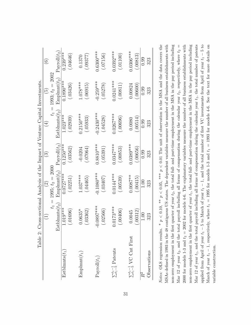
Table 2 presents the results of two sets of cross-sectional analyses. The first three columns

report estimates with a five-year lag between the outcome measures and the predictors—in

other words, for an analysis using the attributes of MSAs in 1995 to predict the number

of firms, employment, and aggregate income in 2000. The next three columns present the

estimates from a set of models using a nine-year lag, using 1993 values to predict 2002

outcomes. The controls suggest that regions with more innovation in the five years leading

up to t1 experienced faster growth over the next five years in the number of firms, employment

and aggregate income in the region. Venture capital, by comparison, had no apparent effect

on the number of firms in the region using either the five- or nine-year lag. That does not

imply that venture capital does not increase entrepreneurship, but it does suggest that either

these new firms displace existing firms in the region or they do not survive long on average.

The local supply of venture capital does, on the other hand, appear to increase both em-

ployment and aggregate income in the region. The magnitude of these effects are substantial.

almost uniformly made investments consistent with their stated scopes. We nevertheless restricted theindividual investments used in constructing our count and amount variables to those that fell into thesestages.

12

A doubling in the amount of venture capital invested over the five years leading up to t1

implies a 0.6% increase in employment and a 2.7% rise in aggregate income in the region five

years later. The larger marginal effect of venture capital on income relative to employment

suggests either that venture capital produces particularly well paying jobs or (more likely)

that the greater availability of entrepreneurship and small-firm employment as an outside

option places upward pressure on the wages paid by existing employers. Longer lags, such as

the nine-year lag reported in columns (4) through (6), yield results of almost identical mag-

nitude. Most of the economic benefit of venture capital to the regional economy, therefore,

appears to accrue in the first few years following funding.

These cross-sectional estimates may nonetheless confound the effects of venture capital

with a wide range of other factors that vary from one region to the next. To investigate

these issues further, let us turn to analyses that use longitudinal variation within regions to

identify the effects of venture capital on the economy.

3.2 Fixed effects estimates

Our fixed effects specifications included region fixed effects, to control for time-invariant

characteristics of MSAs that might both attract venture capital and influence entrepreneur-

ship and economic growth. We also included dummy variables for each calendar year to

control for macro-economic factors that might influence the availability of venture capital,

entrepreneurship and economic performance across the country as a whole. The tables below

also report estimates with and without region-specific trends, to capture regional differences

in the average growth rates in entrepreneurship, employment and aggregate income over

13

time. In particular, we estimated a logged form of a standard production function:

ln Yi,t = β1 ln Ii,t−1 + β2 ln Pi,t + β3 ln V Ci,t + φt + ηi + νit + εi,t, (2)

where i and t index the MSA and the year, respectively. As above, Yi,t denotes the various

outcome measures, Ii,t−1 indicates innovation (patent applications), and V Ci,t represents

venture capital activity. The fixed effects models also included a control for regional growth

in the population (Pi,t), a series of indicator variables for each year (φt), MSA fixed effects

(ηi, partialed out), and (in some models) an MSA-specific growth trend (νit). We clustered

the standard errors on MSAs to allow for correlation in the errors within regions across years.

Descriptive statistics for the variables used in the panel analyses appear in Table 1.

We considered three measures of the supply of venture capital: (1) As in the cross-

sectional models, we counted first investments in firms by venture capital firms in the MSA

organized as limited partnerships. (2) Our second measure counted all investments made

during the year by VC firms located in the MSA (again regardless of the location of the

investment target). This measure should also capture the effects of continuing support for

companies that have already received venture capital. (3) We calculated the total amount

of money invested each year by venture capital funds headquartered in each metropolitan

area.9 In essence, this measure weights the investments in the second measure by their size

in dollars to determine whether larger investments have larger effects. Because all three

measures include some regions with no venture capital activity in a year, we added one to

each measure before logging it.

9Although VentureXpert includes relatively complete information on the size of investment rounds (95%of our cases), it does not contain information on the proportion of these rounds contributed by each investor.In the absence of more detailed information, we allocated the total funds invested in a round equally acrossall investors in that round.

14

Entrepreneurship: We first examined the effects of venture capital on the births of new

establishments. The Census Bureau defines a business establishment as a single physical

location where business occurs and for which a firm maintains payroll and employment

records. All firms have at least one establishment, but many firms have more than one. We

used the natural log of establishment births as our measure of entrepreneurship.

Table 3 reports the results of these analyses. The first three columns do not include a

region-specific trend, while the last three do. All of the measures of venture capital have

positive effects on entrepreneurship on the models without controls for region-specific growth

rates. The results nevertheless suggest that first investments have a larger stimulative effect

on entrepreneurship than later investments. A doubling in the number of firms funded im-

plied a 0.78% increase in the number of new establishments. 10 Since the average MSA-year

had four VC-funded companies (and 1839 establishment births in the 0-19 category), the

funding of one additional company appeared to generate roughly three-and-one-half new es-

tablishments. By comparison, a doubling in the number of overall investments corresponded

to a 0.55% increase in new establishments. Larger investments also seemed inefficient in

promoting entrepreneurship; a doubling in the dollars invested implied an increase of only

0.05% in the number of companies. After including MSA-specific trends, moreover, the ef-

fects associated with the total number of investments and with the aggregate amount of

these investments falls substantially, to a level below statistical significance.

In addition to counting the foundings of new firms, however, the new establishments

measure also captures both relocations by existing businesses across MSAs and the opening

of new plants and places of business by existing firms. To distinguish these activities from

10Although one could interpret the log-log coefficients directly as elasticities, we chose not to do so becauseone cannot meaningfully consider small percentage changes in the number of companies funded (only 11 ofthe 329 regions had more than 100 companies funded in any single year).

15

entrepreneurship, we used information on the size of the firm at the time of entry. Based

on the total employment of organizations (i.e. across all business locations), the SBA splits

establishment births into three categories: 0-19 employees, 20-499 employees, and over 500

employees. A large firm establishing a small local branch would appear in the 500+ category

regardless of the number of individuals employed at the local branch. New firms meanwhile

should only appear in the 0-19 employee category (though this category might still include

some relocations or expansions of small existing firms). Once again, we logged the variable

before using it in the regressions.

Table 4 details these analyses. Both the pattern of the results and the magnitude of the

coefficients are essentially the same as those in the previous table. Since births of small firms

account for 75% to 80% of all births in most regions, however, that result is not surprising.

Because small establishment births more clearly capture startups, we nonetheless focus on

these births of small firms as our measure of entrepreneurship for the remainder of the paper.

Although most MSAs have at least one local venture capital firm and therefore contribute

to our estimates, one might worry that outliers account for our results. Notably, California,

Massachusetts and Texas, together, account for a little over half of all venture capital during

the period being analyzed. Table 5, therefore, reports the effect of the number of firms funded

on the number of small firm establishment births for a series of models that systematically

remove MSAs in each of these states – and in the final column, all of them – from the

analysis. The size of the effect appears insensitive to the exclusion of those regions with the

highest volumes of venture capital activity.11

Table 6 explores the temporal structure of the relationship between the supply of venture

capital and the births of small establishments. We began by regressing the number of births

11Similar robustness checks using employment and aggregate income as dependent variables also revealedno sensitivity of the results to the inclusion of specific regions.

16

in the region on the number of firms funded in that year, in the previous year, and in the year

before the previous one. As one would expect, the size of the relationship declines steadily

as the lag grows longer. Although some (unreported) models find a significant relationship

with a one-year lag between venture capital investment and births, the effect always falls

to zero with a two-year lag. In terms of magnitude, these estimates suggest that the VC

funding of an additional firm in the typical MSA would result in the opening of roughly 2.4

firms (including the one funded) in the first year and an additional 1.5 firms in the next year.

At least in terms of the temporal structure, reverse causality does not appear a concern.

Employment: Next, we examined the effects of venture capital on overall employment in

the region (Table 7). Once again the first three columns report the models without region-

specific trends and the last three columns report them with the trends. In the models without

region-specific trends, both the number of firms funded and the number of investments had

positive relationships with employment in the region. A doubling in the number of firms

funded in a region implied a 0.51% increase in total employment in the region, while a

doubling in the number of total investments corresponded to a 0.35% rise in employment.

These effects nevertheless decline substantially in magnitude once region-specific trends have

been included in the models. In those models, for example, a doubling in the number of firms

funded implied a 0.24% increase in total employment. As in the entrepreneurship models,

follow-on investments and larger investments appear inefficient in promoting employment

relative to first investments in firms.

Translating those effect sizes into absolute numbers, one would expect the funding of one

additional firm by venture capitalists to result in roughly 157 more full-time-equivalent jobs

for the typical region. In the parallel model of firm births with region-specific time trends

(Table 4, model 4), this same funding of an additional firm implies 2.4 new establishments.

17

If all of these jobs appeared in the firms stimulated by venture capital, therefore, the typical

new venture would employ more than 60 people. Since that number far exceeds the average

size of these ventures, it suggests that at least some of the gains in employment must accrue

to existing firms in the region.

Aggregate income: Finally, we considered the effects of venture capital on the total wage

bill for the region (Table 8). In these models, venture capital has positive and significant

effects across all six models—using all three measures of venture capital and both with

and without controls for region-specific trends. The coefficients from the models with MSA

trends nevertheless suggest must weaker relationships between the supply of venture capital

and aggregate income. Although first investments and subsequent investments have similar

size effects, larger investments appear less efficient in producing wage growth. Whereas a

doubling in the number of firms funded or the total number of investments imply a 0.69% or

0.62% rise, respectively, in the total payroll in the region, a doubling in the dollars invested

would correspond to a 0.033% gain in income (in the models including region-specific trends).

In dollar terms, the funding of an additional firm by venture capital would correspond to

an increase of $14.3 million in the wage bill for the region. Since the average venture capital

investment deploys only $2.5 million in capital, this income effect suggests that venture

capital investments produce a high social return. If all of this income growth stemmed from

the incomes associated with the 157 jobs created – either directly or indirectly – by that

investment, then it would imply that the average job produced by venture capital had a total

compensation of about $91,000.

18

3.3 Fixed effects IV estimates

Though the fixed effects estimates also suggest that venture capital promotes entrepreneur-

ship, employment and income growth, their validity nonetheless rests on an assumption that

the supply of venture capital does not itself depend on entrepreneurship. As noted above,

however, that seems unlikely. Venture capitalists choosing a region in which to locate their

offices would presumably find places with more entrepreneurial activity more attractive, and

even if venture capitalists tend to emerge out of local communities, their interest in raising –

and ability to raise – funds may well depend on perceptions of the degree to which the region

offers attractive investment opportunities. This endogeneity would bias our OLS estimates.

To address these potential endogeneity problems, we also identified the effect using an

instrumental variable (IV).12 Our specification of the IV models follows that described in

equation (2), except that we instrument the supply of venture capital. In the IV models

reported, we focus on the number of firms funded as our measure of venture capital activity

because it has provided the most consistent effects in the cross-sectional and OLS longitudinal

models. We used the LIML estimator for these models because of its greater robustness over

2SLS in terms of removing the OLS bias from the estimates (Stock and Yogo 2005).13

Our instrument, LP Returns, relies on the demand for alternative assets by limited part-

ners. Institutional investors generally have an investing strategy that depends in part on

an optimal allocation of assets across classes (e.g., 60% equity, 30% fixed income, and 10%

alternative assets). The managers of these funds regularly rebalance their portfolios to main-

tain allocations close to these optimal mixes. When the endowments they manage earn high

12Although we do not report these models, we also estimated a set of models using the instrument suggestedby Gompers and Lerner (2000): Inflows into LBO funds in an MSA. Estimates with that instrument yieldedsubstantively equivalent results. We nonetheless prefer LP Returns as an instrument because it predictsmore of the variation in the supply of venture capital and because it is more plausibly exogenous to regionaleconomic activity.

13We estimated all IV models using the xtivreg2 module in Stata 10 (Schaffer 2005).

19

returns, they need to shift assets to venture capital to maintain their asset allocations.14

Investments in VC funds should therefore correlate highly with lagged endowment returns.15

But these institutional investors rarely invest directly in startups, so their returns should

not have a direct effect on entrepreneurship.

Although this relationship should hold at the national level, the usefulness of the instru-

ment as a source of exogenous variation in the regional supply of venture capital depends

also on an assumption that institutional investors have a tendency to invest in locally-

headquartered private equity funds. Such a home bias might exist for a variety of reasons:

Institutional investors might feel more comfortable investing near to home and they more

probably have had prior interactions with the managers of local funds. Regardless of the

reasons, this assumption appears to hold. In our sample, the unconditional probability of

an LP investing in a fund located in the same MSA is roughly double the probability of it

investing in a fund located in an adjacent area and more than six times the probability of it

investing in one further away.

To estimate the effect that rebalancing might have on the local availability of venture

capital, we obtained average annual returns data for college and university endowments,

an important class of limited partners, from The Chronicle of Higher Education. We then

weighted that measure for each region by multiplying these average national returns by the

logged count of institutional investors in the region that had invested in venture capital at

least ten years prior to the focal year (adding one to avoid zeros). The ten-year lag should

remove endogeneity that might result from institutional investors initiating investment in

14Due to the finite maturity of VC investments, the flow of assets to venture capital increases with portfolioreturns, even when VC investments outperform other assets in the portfolio.

15Though one might worry that attractive venture capital investments could drive these returns, becauseventure capital accounts for only a very small portion of institutional investors’ portfolios – less than 1% onaverage (Blumenstyk 2008) – reverse causality is not an issue here.

20

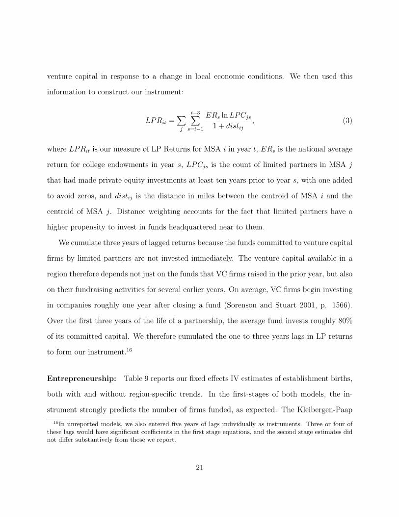
venture capital in response to a change in local economic conditions. We then used this

information to construct our instrument:

LPRit =∑j

t−3∑s=t−1

ERs ln LPCjs

1 + distij, (3)

where LPRit is our measure of LP Returns for MSA i in year t, ERs is the national average

return for college endowments in year s, LPCjs is the count of limited partners in MSA j

that had made private equity investments at least ten years prior to year s, with one added

to avoid zeros, and distij is the distance in miles between the centroid of MSA i and the

centroid of MSA j. Distance weighting accounts for the fact that limited partners have a

higher propensity to invest in funds headquartered near to them.

We cumulate three years of lagged returns because the funds committed to venture capital

firms by limited partners are not invested immediately. The venture capital available in a

region therefore depends not just on the funds that VC firms raised in the prior year, but also

on their fundraising activities for several earlier years. On average, VC firms begin investing

in companies roughly one year after closing a fund (Sorenson and Stuart 2001, p. 1566).

Over the first three years of the life of a partnership, the average fund invests roughly 80%

of its committed capital. We therefore cumulated the one to three years lags in LP returns

to form our instrument.16

Entrepreneurship: Table 9 reports our fixed effects IV estimates of establishment births,

both with and without region-specific trends. In the first-stages of both models, the in-

strument strongly predicts the number of firms funded, as expected. The Kleibergen-Paap

16In unreported models, we also entered five years of lags individually as instruments. Three or four ofthese lags would have significant coefficients in the first stage equations, and the second stage estimates didnot differ substantively from those we report.

21

rk Wald statistic (Kleibergen and Paap 2006) – reported as “KP Wald” with the second-

stage estimates in the IV tables – tests directly whether our instrument predicts a sufficient

amount of the variance in the endogenous variables to identify our equations. For LIML

estimation with one instrument and one endogenous variable, Stock and Yogo (2005) report

a critical value of 16.38 for the IV estimates to have no more than 10% of the bias of the

OLS estimates.17 For both models, the KP Wald statistic far exceeds this critical value.

Assessing the results, in both models, the supply of venture capital has a positive relation-

ship to the number of new establishments. The point estimate of this effect has increased in

the IV estimation—nearly tripling in magnitude in the model without region-specific trends

and nearly quadrupling in magnitude in the model with them. Because of the larger stan-

dard errors, the OLS estimates nevertheless are within the 95% confidence intervals of the

IV estimates. In the model with the region-specific trends, the IV estimates suggest that a

doubling in the number of firms funded would result in a 2.2% increase in the number of new

establishments by organizations with 0-19 employees (roughly seven new establishments per

company funded in an MSA with an average supply of venture capital and the mean number

of new establishments).

Employment: Table 10 reports parallel results of fixed effects IV estimates of employment.

Once again, the instrument appears well behaved. The Kleibergen-Paap Wald statistics

again suggest that the first stages have sufficient strength to identify VC investment counts

(though the statistic suggests that the instrument becomes much weaker in the model that

includes region-specific trends).

In the model without region-specific trends, the IV point estimate is nearly identical

17Although we do not report it, the LM version of the Kleibergen-Paap test yielded equivalent results.We should also note that though the Kleibergen-Paap Wald statistic is robust to within-cluster correlationin the errors, Stock and Yogo (2005) only tabulated critical values for the case of uncorrelated errors.

22

to that obtained in the OLS fixed effects model. In the model with region-specific trends,

however, the point estimate of the effect of venture capital on employment increases almost

by an order of magnitude (from a doubling in firms funded implying a 0.24% increase in

employment to it implying a 1.4% rise in employment). In both cases, however, the OLS

point estimates again fall within the 95% confidence intervals of the IV estimates. Given

the smaller Kleibergen-Paap Wald statistic in this model and this enormous increase in the

magnitude of the estimated effect, we nonetheless worry that the effect size in the model

with region-specific trends may reflect the weakness of the instrument in that specification.

Aggregate income: Table 11 finally reports estimates of the effects of venture capital on

the overall compensation in a region using an instrument to identify the supply of venture

capital. The instrument again appears well behaved in both models. Again, the IV estima-

tion produced significantly larger estimates of the effect than the fixed effects regressions—

roughly triple the size in the models without region-specific trends and fives times the size

in the ones with them. If all of the increase in aggregate income resulted from the jobs

predicted in model 10-2, then the average employee in one of these jobs created by ven-

ture capital would need to receive compensation on the order of $83,000 per year. As with

the OLS estimates, that number seems reasonable in magnitude, thus the employment and

aggregate income results appear consistent in the magnitude of the effects that they suggest.

4 Discussion

We find that increases in the supply of venture capital in an MSA stimulate the production of

new firms in the region. This effect appears consistent with either of two mechanisms. One,

would-be entrepreneurs in need of capital may incorporate the availability of such capital into

23

their calculations when trying to decide whether to start their firms. Two, the firms that

VC firms finance may serve as inspiration and training grounds for future entrepreneurs.

We further find that an expanded supply of venture capital appears to raise employment

and aggregate income in a region. At least some of these employment and income effects

probably stem from the fact that venture capital allows entrepreneurs to create value by

pursuing ideas that they otherwise could not. Our results remain robust to estimation with

an instrumental variable.

Our results seem quite consistent with the general notion that an expansion in finan-

cial intermediation improves the allocation of capital and therefore can stimulate growth

(Greenwood and Jovanovic 1990). Venture capital firms fill a niche that allows the necessary

capital to reach some of the least developed and most uncertain ideas. Hence, alternative

forms of financing, such as banks, cannot easily substitute for venture capital in its absence.

Individual investors (“angels”), moreover, may lack the requisite skills and experience to

choose and incubate these young companies effectively (though the relative efficiency of an-

gel investments versus venture capital falls outside the scope of this analysis and deserves

greater research attention).

But our results do not imply that regions would benefit from an unlimited supply of

venture capital. Because we find an elasticity of less than one, our results imply decreasing

returns to the availability of venture capital. We can moreover use the estimates from the

dollars invested on the wage bill (model 8-3) to place a minimum on the optimal supply

of venture capital. Although the wage bill does not incorporate all capital gains, the point

at which an additional dollar of venture capital would yield less than an additional dollar

in wages at least provides a lower bound on the optimal supply of venture capital. In

other words, we calculate the point at which the change in the wages equals the change in

24

investment (∆Wage = ∆V CInvestAmt). For the average MSA, this calculation yields a

sum of roughly $7 million dollars (with a 90% confidence interval ranging from $400,000 to

$14 million dollars).

When one adjusts for the fact that smaller regions would require less venture capital and

larger regions would require more, our estimates suggest that only 195 of the 329 MSAs in our

analysis ever exceed this minimum bound. Only 15 of the areas – Atlanta, Bergen-Passaic

(NJ), Boston, Boulder, Bridgeport (CT), Dallas, Lowell (MA), Middlesex (NJ), Oakland,

Orange County, San Diego, San Francisco, San Jose, Seattle and Stamford (CT) – exceed it

for every year in our window. Our findings therefore suggest that most metropolitan regions

in the United States could benefit from an expansion in venture capital.

Given this inadequate supply, several questions naturally arise. First, why do some

regions have an undersupply of venture capital? Does it stem from an unwillingness to

invest in venture capital among local institutions or from a shortage of experienced venture

capitalists? Second, can public policy correct this situation, and if so, how? Obviously, the

answers to the second question depend in large part on those to the first.

Another interesting line of inquiry would consider whether the efficiency of venture cap-

ital depends on other factors. For example, to the extent that our results stem from the

expectations of capital constrained entrepreneurs, then the supply of venture capital should

have the largest effect in regions (or at times) in which alternative forms of financing are

dear. This question also has clear policy relevance. Government programs to expand the

supply of venture capital have met with mixed success. At one extreme, the Israeli model

has almost uniformly been praised and offered as an example of best practices. At the other,

both the Canadian and German models appear to have had limited success and may have

even stunted the development of venture capital in those regions. Although the focus to

25

date has primarily been on the internal design of these programs, variation across countries

in the success of these programs may also stem from differences in complementary factors

within these jurisdictions.

References

Blanchflower, David G and Andrew J Oswald. 1998. “What makes an entrepreneur?” Jour-

nal of Labor Economics 16:26–60.

Blumenstyk, Goldie. 2008. “Endowments savor big gains but lower their sights.” The Chron-

icle of Higher Education 54:A1.

Bottazzi, Laura and Marco Da Rin. 2002. “Venture capital in Europe and the financing of

innovative companies.” Economic Policy 17:229–269.

Chen, Peng, Gary T Baierl, and Paul D Kaplan. 2002. “Venture capital and its role in

strategic asset allocation.” Journal of Portfolio Management 28:83–89.

Cochrane, John H. 2005. “The risk and return of venture capital.” Journal of Financial

Economics 75.

Cumming, Douglas J and Jeffrey G MacIntosh. 2007. “Mutual funds that invest in pri-

vate equity? An analysis of labour-sponsored investment funds.” Cambridge Journal of

Economics 31:445–487.

Engel, Dirk and Max Keilbach. 2007. “Firm-level implications of early stage venture capital

investment - an empirical investigation.” Journal of Empirical Finance 14:150–167.

26

Evans, David S and Boyan Jovanovic. 1989. “An estimated model of entrepreneurial choice

under liquidity constraints.” Journal of Political Economy 97:808–827.

Gans, Joshua S and Scott Stern. 2003. “When does funding research by smaller firms bear

fruit? Evidence from the SBIR program.” Economics of Innovation and New Technology

12:361–384.

Gilson, Ronald J. 2003. “Engineering a venture capital market: Lessons from the American

experience.” Stanford Law Review 55:1067–1104.

Glaeser, Edward L., Hedi D. Kallal, Jose A. Scheinkman, and Andrei Shleifer. 1992. “Growth

in cities.” Journal of Political Economy 100:1126–1152.

Gompers, Paul and Josh Lerner. 2000. “Money Chasing Deals? The Impact of Fund Inflows

on Private Equity Valuations.” Journal of Financial Economics 55:281–325.

Gompers, Paul A and Josh Lerner. 1998. “What drives venture capital fundraising?” Brook-

ings Papers on Economic Activity – Microeconomics pp. 149–204.

Greenwood, Jeremy and Boyan Jovanovic. 1990. “Financial development, growth, and the

distribution of income.” Journal of Political Economy 98:1076–1107.

Hasan, Iftekhar and Haizhi Wang. 2006. “The role of venture capital on innovation, new

business formation, and economic growth.” Presented at the 2006 FMA Annual Meeting.

Jain, Bharat A. and Omesh Kini. 1995. “Venture capitalist participation and the post-issue

operating performance of IPO firms.” Managerial and Decision Economics 16:593–606.

Keuschnigg, Christian. 2004. “Venture capital backed growth.” Journal of Economic Growth

9:239–261.

27

Kleibergen, F. and R. Paap. 2006. “Generalized Reduced Rank Tests Using the Singular

Value Decomposition.” Journal of Econometrics 133:97–126.

Kortum, Samuel and Josh Lerner. 2000. “Assessing the Contribution of Venture Capital to

Innovation.” RAND Journal of Economics 31:674–692.

Rodrik, Dani, Arvind Subramanian, and Francesco Trebbi. 2004. “Institutions rule: The

primacy of institutions over geography and integration in economic development.” Journal

of Economic Growth 9:131–165.

Rosenthal, Stuart S. and William C. Strange. 2003. “Geography, industrial organization,

and agglomeration.” Review of Economics and Statistics 85:377–393.

Schaffer, Mark E. 2005. “Xtivreg2: Stata Module to Perform Extended Iv/2sls, Gmm

and Ac/Hac, Liml and K-Class Regression for Panel Data Models.” Statistical Software

Components, Boston College Department of Economics.

Schumpeter, Joseph A. 1934. The Theory of Economic Development . Cambridge, MA:

Harvard University Press.

Sorensen, Morten. 2007. “How smart is smart money? A two-sided matching model of

venture capital.” Journal of Finance 62:2725–2762.

Sorenson, Olav and Pino G. Audia. 2000. “The social structure of entrepreneurial activ-

ity: Geographic concentration of footwear production in the United States, 1940-1989.”

American Journal of Sociology 106:424–462.

Sorenson, Olav and Toby E. Stuart. 2001. “Syndication networks and the spatial distribution

of venture capital investments.” American Journal of Sociology 106:1546–1588.

28

Stock, J. H. and M. Yogo. 2005. “Testing for Weak Instruments in Linear IV Regression.” In

Identification and Inference for Econometric Models: Essays in Honor of Thomas Rothen-

berg , edited by D. W. K. Andrews and J. H. Stock, pp. 80–108. Cambridge: Cambridge

University Press.

29

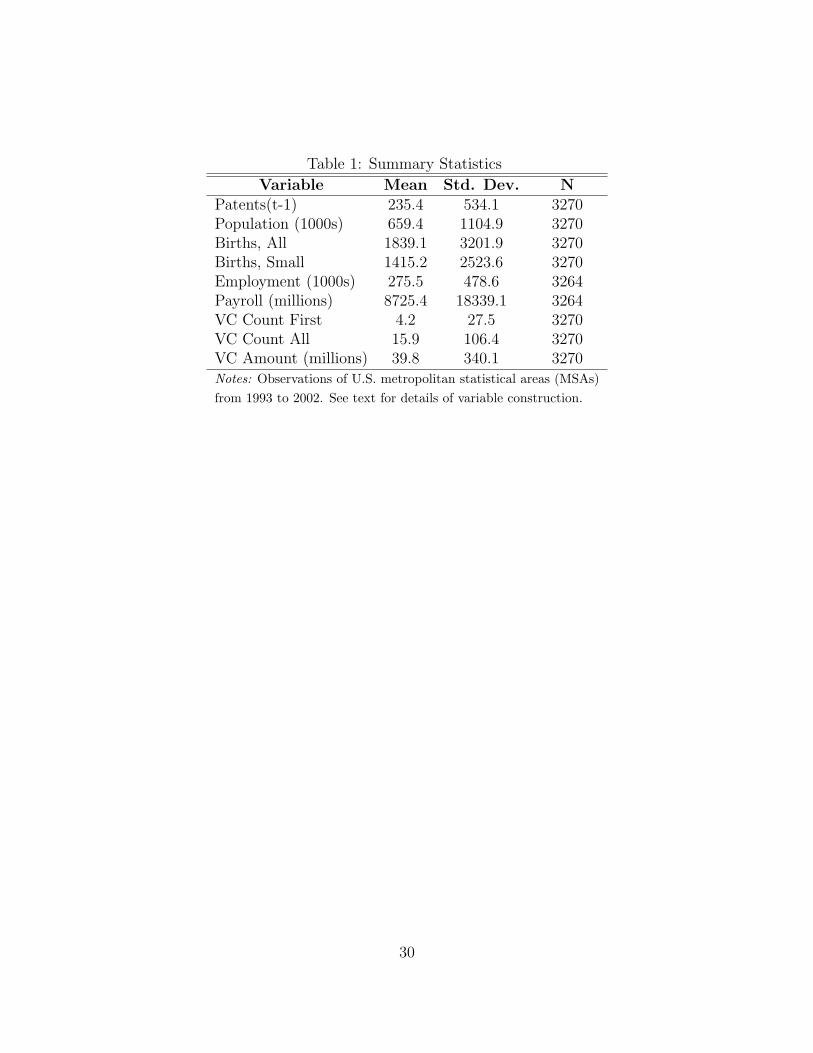
Table 1: Summary Statistics

Variable Mean Std. Dev. NPatents(t-1) 235.4 534.1 3270Population (1000s) 659.4 1104.9 3270Births, All 1839.1 3201.9 3270Births, Small 1415.2 2523.6 3270Employment (1000s) 275.5 478.6 3264Payroll (millions) 8725.4 18339.1 3264VC Count First 4.2 27.5 3270VC Count All 15.9 106.4 3270VC Amount (millions) 39.8 340.1 3270Notes: Observations of U.S. metropolitan statistical areas (MSAs)from 1993 to 2002. See text for details of variable construction.

30

Tab

le2:

Cro

ss-s

ecti

onal

Anal

ysi

sof

the

Impac

tof

Ven

ture

Cap

ital

Inve

stm

ents

.

(1)

(2)

(3)

(4)

(5)

(6)

t 1=

1995

;t 2

=20

00t 1

=19

93;t 2

=20

02E

stblm

nts

(t2)

Em

plm

nt(

t 2)

Pay

roll(t

2)

Est

blm

nts

(t2)

Em

plm

nt(

t 2)

Pay

roll(t

2)

Est

blm

nts

(t1)

1.01

9***

0.07

27**

*0.

1250

***

1.02

3***

0.18

90**

*0.

239*

**(.

0169

6)(.

0225

1)(.03

562)

(.02

939)

(.03

426)

(.04

646)

Em

plm

nt(

t 1)

0.06

35*

1.03

7***

-0.0

204

0.21

50**

*1.

078*

**0.

1370

(.03

362)

(.04

465)

(.07

064)

(.05

933)

(.06

915)

(.09

377)

Pay

roll(t

1)

-0.0

897*

**-0

.108

0***

0.88

10**

*-0

.243

0***

-0.2

59**

*0.

6300

***

(.02

566)

(.03

407)

(.05

391)

(.04

528)

(.05

278)

(.07

156)

∑ t 1−1

t 1−

5Pat

ents

0.01

73**

*0.

0144

***

0.03

47**

*0.

0267

***

0.02

41**

*0.

0392

***

(.00

406)

(.00

539)

(.00

853)

(.00

696)

(.00

811)

(.01

100)

∑ t 1−1

t 1−

5V

CC

nt

First

0.00

450.

0087

**0.

0389

***

0.00

800.

0082

40.

0306

***

(.00

312)

(.00

415)

(.00

656)

(.00

514)

(.00

600)

(.00

813)

R2

1.00

1.00

0.99

0.99

0.99

0.99

Obse

rvat

ions

323

323

323

323

323

323

Not

es:

OLS

regr

essi

onre

sult

s.*

p<

0.10

,**

p<

0.05

,**

*p

<0.

01T

heun

itof

obse

rvat

ion

isth

eM

SAan

dth

eda

taco

vers

the

MSA

sde

fined

in19

93in

the

48co

ntig

uous

US

stat

es.

The

depe

nden

tva

riab

les

mea

sure

the

num

ber

ofal

lbus

ines

ses

tabl

ishm

ents

wit

hno

n-ze

roem

ploy

men

tin

the

first

quar

ter

ofye

art 2

,the

tota

lful

l-an

dpa

rt-t

ime

empl

oym

ent

inth

eM

SAin

the

pay

peri

odin

clud

ing

Mar

12of

year

t 2,

and

the

tota

lpa

yrol

lin

clud

ing

all

form

sof

com

pens

atio

ndu

ring

the

cale

ndar

year

t 2,

resp

ecti

vely

,w

here

t 2=

2000

for

mod

els

1-3

and

t 2=

2002

for

mod

els

4-6.

The

expl

anat

ory

vari

able

sm

easu

reth

enu

mbe

rof

allb

usin

ess

esta

blis

hmen

tsw

ith

non-

zero

empl

oym

ent

inth

efir

stqu

arte

rof

year

t 1,t

heto

talf

ull-

and

part

-tim

eem

ploy

men

tin

the

MSA

inth

epa

ype

riod

incl

udin

gM

ar12

ofye

art 1

,an

dth

eto

talpa

yrol

lin

clud

ing

allfo

rms

ofco

mpe

nsat

ion

duri

ngth

eca

lend

arye

art 1

,th

eto

talnu

mbe

rof

pate

nts

appl

ied

from

Apr

ilof

year

t 1−

5to

Mar

chof

year

t 1−

1,an

dth

eto

talnu

mbe

rof

first

VC

inve

stm

ents

from

Apr

ilof

year

t 1−

5to

Mar

chof

year

t 1−

1,re

spec

tive

ly,

whe

ret 1

=19

95fo

rm

odel

s1-

3an

dt 1

=19

93fo

rm

odel

s4-

6.Se

eth

ete

xtfo

rm

ore

deta

ilson

vari

able

cons

truc

tion

.

31

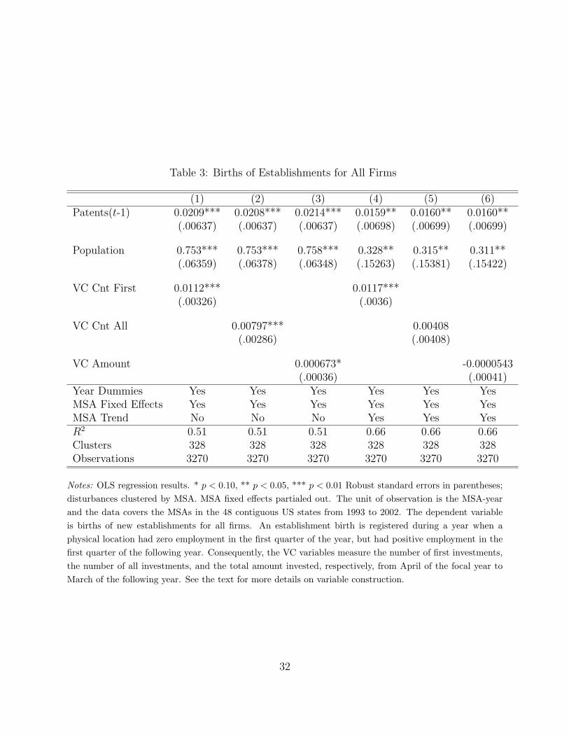
Table 3: Births of Establishments for All Firms

(1) (2) (3) (4) (5) (6)Patents(t-1) 0.0209*** 0.0208*** 0.0214*** 0.0159** 0.0160** 0.0160**

(.00637) (.00637) (.00637) (.00698) (.00699) (.00699)

Population 0.753*** 0.753*** 0.758*** 0.328** 0.315** 0.311**(.06359) (.06378) (.06348) (.15263) (.15381) (.15422)

VC Cnt First 0.0112*** 0.0117***(.00326) (.0036)

VC Cnt All 0.00797*** 0.00408(.00286) (.00408)

VC Amount 0.000673* -0.0000543(.00036) (.00041)

Year Dummies Yes Yes Yes Yes Yes YesMSA Fixed Effects Yes Yes Yes Yes Yes YesMSA Trend No No No Yes Yes YesR2 0.51 0.51 0.51 0.66 0.66 0.66Clusters 328 328 328 328 328 328Observations 3270 3270 3270 3270 3270 3270

Notes: OLS regression results. * p < 0.10, ** p < 0.05, *** p < 0.01 Robust standard errors in parentheses;disturbances clustered by MSA. MSA fixed effects partialed out. The unit of observation is the MSA-yearand the data covers the MSAs in the 48 contiguous US states from 1993 to 2002. The dependent variableis births of new establishments for all firms. An establishment birth is registered during a year when aphysical location had zero employment in the first quarter of the year, but had positive employment in thefirst quarter of the following year. Consequently, the VC variables measure the number of first investments,the number of all investments, and the total amount invested, respectively, from April of the focal year toMarch of the following year. See the text for more details on variable construction.

32

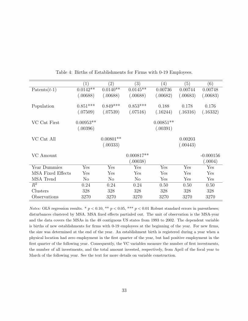
Table 4: Births of Establishments for Firms with 0-19 Employees.

(1) (2) (3) (4) (5) (6)Patents(t-1) 0.0142** 0.0140** 0.0145** 0.00736 0.00744 0.00748

(.00688) (.00688) (.00688) (.00682) (.00683) (.00683)

Population 0.851*** 0.849*** 0.853*** 0.188 0.178 0.176(.07509) (.07539) (.07516) (.16244) (.16316) (.16332)

VC Cnt First 0.00953** 0.00851**(.00396) (.00391)

VC Cnt All 0.00801** 0.00203(.00333) (.00443)

VC Amount 0.000817** -0.000156(.00038) (.0004)

Year Dummies Yes Yes Yes Yes Yes YesMSA Fixed Effects Yes Yes Yes Yes Yes YesMSA Trend No No No Yes Yes YesR2 0.24 0.24 0.24 0.50 0.50 0.50Clusters 328 328 328 328 328 328Observations 3270 3270 3270 3270 3270 3270

Notes: OLS regression results. * p < 0.10, ** p < 0.05, *** p < 0.01 Robust standard errors in parentheses;disturbances clustered by MSA. MSA fixed effects partialed out. The unit of observation is the MSA-yearand the data covers the MSAs in the 48 contiguous US states from 1993 to 2002. The dependent variableis births of new establishments for firms with 0-19 employees at the beginning of the year. For new firms,the size was determined at the end of the year. An establishment birth is registered during a year when aphysical location had zero employment in the first quarter of the year, but had positive employment in thefirst quarter of the following year. Consequently, the VC variables measure the number of first investments,the number of all investments, and the total amount invested, respectively, from April of the focal year toMarch of the following year. See the text for more details on variable construction.

33

Table 5: High-VC-Activity States and Small Establishment Births.

(1) (2) (3) (4) (5)All No CA No MA No TX No CA,MA,TX

Patents(t-1) 0.00736 0.00669 0.00771 0.00691 0.00645(.00682) (.00705) (.00682) (.00743) (.00769)

Population 0.188 0.0997 0.175 0.323* 0.223(.16244) (.17489) (.16353) (.17651) (.19601)

VC Cnt First 0.00851** 0.00770* 0.0108*** 0.00849** 0.0104**(.00391) (.00407) (.00383) (.00411) (.00417)

Year Dummies Yes Yes Yes Yes YesMSA Fixed Effects Yes Yes Yes Yes YesMSA Trend Yes Yes Yes Yes YesR2 0.50 0.50 0.53 0.50 0.54Clusters 328 303 317 301 265Observations 3270 3020 3160 3000 2640

Notes: OLS regression results. * p < 0.10, ** p < 0.05, *** p < 0.01 Robust standard errors in parentheses;disturbances clustered by MSA. MSA fixed effects partialed out. The unit of observation is the MSA-yearand the data covers the MSAs in the 48 contiguous US states from 1993 to 2002. The dependent variableis births of new establishments for firms with 0-19 employees at the beginning of the year. For new firms,the size was determined at the end of the year. An establishment birth is registered during a year when aphysical location had zero employment in the first quarter of the year, but had positive employment in thefirst quarter of the following year. Consequently, the VC variable measures the number of first investmentsfrom April of the focal year to March of the following year. Model 1 includes MSAs in all states. Model 2excludes MSAs in California. Model 3 excludes MSAs in Massachusetts. Model 4 excludes MSAs in Texas.Model 5 excludes MSAs in California, Massachusetts, and Texas. See the text for more details on variableconstruction.

34

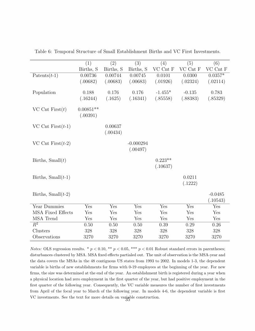
Table 6: Temporal Structure of Small Establishment Births and VC First Investments.

(1) (2) (3) (4) (5) (6)Births, S Births, S Births, S VC Cnt F VC Cnt F VC Cnt F

Patents(t-1) 0.00736 0.00744 0.00745 0.0101 0.0300 0.0357*(.00682) (.00683) (.00683) (.01926) (.02324) (.02114)

Population 0.188 0.176 0.176 -1.455* -0.135 0.783(.16244) (.1625) (.16341) (.85558) (.88383) (.85329)

VC Cnt First(t) 0.00851**(.00391)

VC Cnt First(t-1) 0.00637(.00434)

VC Cnt First(t-2) -0.000294(.00497)

Births, Small(t) 0.223**(.10637)

Births, Small(t-1) 0.0211(.1222)

Births, Small(t-2) -0.0485(.10543)

Year Dummies Yes Yes Yes Yes Yes YesMSA Fixed Effects Yes Yes Yes Yes Yes YesMSA Trend Yes Yes Yes Yes Yes YesR2 0.50 0.50 0.50 0.39 0.29 0.26Clusters 328 328 328 328 328 328Observations 3270 3270 3270 3270 3270 3270

Notes: OLS regression results. * p < 0.10, ** p < 0.05, *** p < 0.01 Robust standard errors in parentheses;disturbances clustered by MSA. MSA fixed effects partialed out. The unit of observation is the MSA-year andthe data covers the MSAs in the 48 contiguous US states from 1993 to 2002. In models 1-3, the dependentvariable is births of new establishments for firms with 0-19 employees at the beginning of the year. For newfirms, the size was determined at the end of the year. An establishment birth is registered during a year whena physical location had zero employment in the first quarter of the year, but had positive employment in thefirst quarter of the following year. Consequently, the VC variable measures the number of first investmentsfrom April of the focal year to March of the following year. In models 4-6, the dependent variable is firstVC investments. See the text for more details on variable construction.35

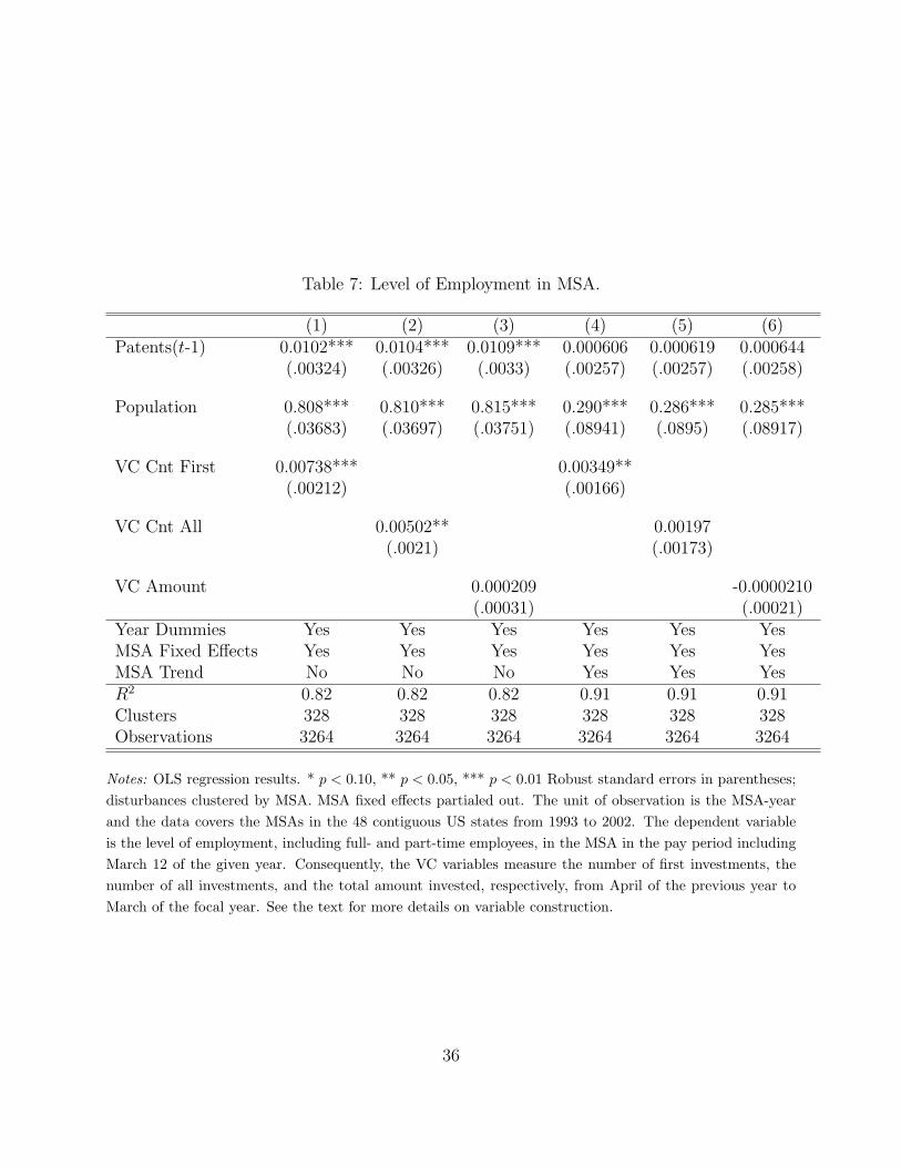
Table 7: Level of Employment in MSA.

(1) (2) (3) (4) (5) (6)Patents(t-1) 0.0102*** 0.0104*** 0.0109*** 0.000606 0.000619 0.000644

(.00324) (.00326) (.0033) (.00257) (.00257) (.00258)

Population 0.808*** 0.810*** 0.815*** 0.290*** 0.286*** 0.285***(.03683) (.03697) (.03751) (.08941) (.0895) (.08917)

VC Cnt First 0.00738*** 0.00349**(.00212) (.00166)

VC Cnt All 0.00502** 0.00197(.0021) (.00173)

VC Amount 0.000209 -0.0000210(.00031) (.00021)

Year Dummies Yes Yes Yes Yes Yes YesMSA Fixed Effects Yes Yes Yes Yes Yes YesMSA Trend No No No Yes Yes YesR2 0.82 0.82 0.82 0.91 0.91 0.91Clusters 328 328 328 328 328 328Observations 3264 3264 3264 3264 3264 3264

Notes: OLS regression results. * p < 0.10, ** p < 0.05, *** p < 0.01 Robust standard errors in parentheses;disturbances clustered by MSA. MSA fixed effects partialed out. The unit of observation is the MSA-yearand the data covers the MSAs in the 48 contiguous US states from 1993 to 2002. The dependent variableis the level of employment, including full- and part-time employees, in the MSA in the pay period includingMarch 12 of the given year. Consequently, the VC variables measure the number of first investments, thenumber of all investments, and the total amount invested, respectively, from April of the previous year toMarch of the focal year. See the text for more details on variable construction.

36

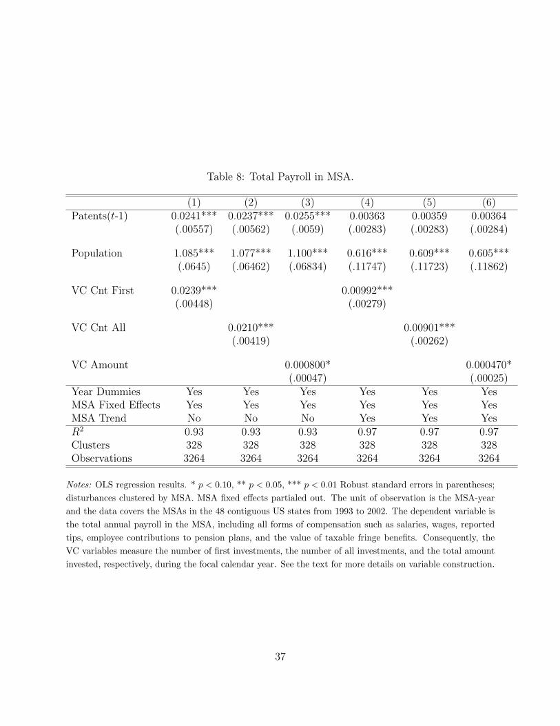
Table 8: Total Payroll in MSA.

(1) (2) (3) (4) (5) (6)Patents(t-1) 0.0241*** 0.0237*** 0.0255*** 0.00363 0.00359 0.00364

(.00557) (.00562) (.0059) (.00283) (.00283) (.00284)

Population 1.085*** 1.077*** 1.100*** 0.616*** 0.609*** 0.605***(.0645) (.06462) (.06834) (.11747) (.11723) (.11862)

VC Cnt First 0.0239*** 0.00992***(.00448) (.00279)

VC Cnt All 0.0210*** 0.00901***(.00419) (.00262)

VC Amount 0.000800* 0.000470*(.00047) (.00025)

Year Dummies Yes Yes Yes Yes Yes YesMSA Fixed Effects Yes Yes Yes Yes Yes YesMSA Trend No No No Yes Yes YesR2 0.93 0.93 0.93 0.97 0.97 0.97Clusters 328 328 328 328 328 328Observations 3264 3264 3264 3264 3264 3264

Notes: OLS regression results. * p < 0.10, ** p < 0.05, *** p < 0.01 Robust standard errors in parentheses;disturbances clustered by MSA. MSA fixed effects partialed out. The unit of observation is the MSA-yearand the data covers the MSAs in the 48 contiguous US states from 1993 to 2002. The dependent variable isthe total annual payroll in the MSA, including all forms of compensation such as salaries, wages, reportedtips, employee contributions to pension plans, and the value of taxable fringe benefits. Consequently, theVC variables measure the number of first investments, the number of all investments, and the total amountinvested, respectively, during the focal calendar year. See the text for more details on variable construction.

37

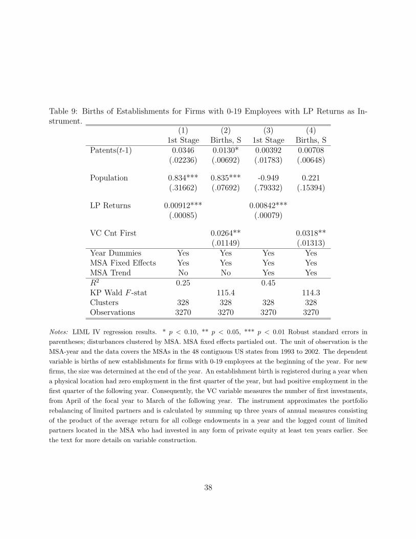
Table 9: Births of Establishments for Firms with 0-19 Employees with LP Returns as In-strument.

(1) (2) (3) (4)1st Stage Births, S 1st Stage Births, S

Patents(t-1) 0.0346 0.0130* 0.00392 0.00708(.02236) (.00692) (.01783) (.00648)

Population 0.834*** 0.835*** -0.949 0.221(.31662) (.07692) (.79332) (.15394)

LP Returns 0.00912*** 0.00842***(.00085) (.00079)

VC Cnt First 0.0264** 0.0318**(.01149) (.01313)

Year Dummies Yes Yes Yes YesMSA Fixed Effects Yes Yes Yes YesMSA Trend No No Yes YesR2 0.25 0.45KP Wald F -stat 115.4 114.3Clusters 328 328 328 328Observations 3270 3270 3270 3270

Notes: LIML IV regression results. * p < 0.10, ** p < 0.05, *** p < 0.01 Robust standard errors inparentheses; disturbances clustered by MSA. MSA fixed effects partialed out. The unit of observation is theMSA-year and the data covers the MSAs in the 48 contiguous US states from 1993 to 2002. The dependentvariable is births of new establishments for firms with 0-19 employees at the beginning of the year. For newfirms, the size was determined at the end of the year. An establishment birth is registered during a year whena physical location had zero employment in the first quarter of the year, but had positive employment in thefirst quarter of the following year. Consequently, the VC variable measures the number of first investments,from April of the focal year to March of the following year. The instrument approximates the portfoliorebalancing of limited partners and is calculated by summing up three years of annual measures consistingof the product of the average return for all college endowments in a year and the logged count of limitedpartners located in the MSA who had invested in any form of private equity at least ten years earlier. Seethe text for more details on variable construction.

38

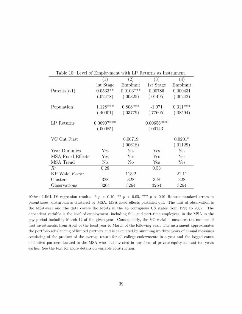
Table 10: Level of Employment with LP Returns as Instrument.

(1) (2) (3) (4)1st Stage Emplmnt 1st Stage Emplmnt

Patents(t-1) 0.0533** 0.0103*** 0.00786 0.000431(.02478) (.00325) (.01495) (.00242)

Population 1.128*** 0.808*** -1.071 0.311***(.40001) (.03779) (.77605) (.08594)

LP Returns 0.00907*** 0.00656***(.00085) (.00143)

VC Cnt First 0.00719 0.0201*(.00618) (.01129)

Year Dummies Yes Yes Yes YesMSA Fixed Effects Yes Yes Yes YesMSA Trend No No Yes YesR2 0.28 0.53KP Wald F -stat 113.2 21.11Clusters 328 328 328 328Observations 3264 3264 3264 3264

Notes: LIML IV regression results. * p < 0.10, ** p < 0.05, *** p < 0.01 Robust standard errors inparentheses; disturbances clustered by MSA. MSA fixed effects partialed out. The unit of observation isthe MSA-year and the data covers the MSAs in the 48 contiguous US states from 1993 to 2002. Thedependent variable is the level of employment, including full- and part-time employees, in the MSA in thepay period including March 12 of the given year. Consequently, the VC variable measures the number offirst investments, from April of the focal year to March of the following year. The instrument approximatesthe portfolio rebalancing of limited partners and is calculated by summing up three years of annual measuresconsisting of the product of the average return for all college endowments in a year and the logged countof limited partners located in the MSA who had invested in any form of private equity at least ten yearsearlier. See the text for more details on variable construction.

39

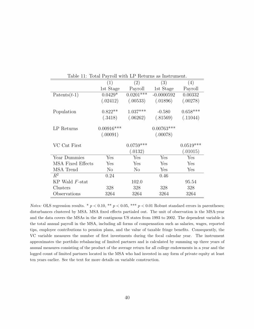
Table 11: Total Payroll with LP Returns as Instrument.

(1) (2) (3) (4)1st Stage Payroll 1st Stage Payroll

Patents(t-1) 0.0429* 0.0201*** -0.0000592 0.00332(.02412) (.00533) (.01896) (.00278)

Population 0.822** 1.037*** -0.580 0.658***(.3418) (.06262) (.81569) (.11044)

LP Returns 0.00916*** 0.00763***(.00091) (.00078)

VC Cnt First 0.0759*** 0.0519***(.0132) (.01015)

Year Dummies Yes Yes Yes YesMSA Fixed Effects Yes Yes Yes YesMSA Trend No No Yes YesR2 0.24 0.46KP Wald F -stat 102.0 95.54Clusters 328 328 328 328Observations 3264 3264 3264 3264

Notes: OLS regression results. * p < 0.10, ** p < 0.05, *** p < 0.01 Robust standard errors in parentheses;disturbances clustered by MSA. MSA fixed effects partialed out. The unit of observation is the MSA-yearand the data covers the MSAs in the 48 contiguous US states from 1993 to 2002. The dependent variable isthe total annual payroll in the MSA, including all forms of compensation such as salaries, wages, reportedtips, employee contributions to pension plans, and the value of taxable fringe benefits. Consequently, theVC variable measures the number of first investments during the focal calendar year. The instrumentapproximates the portfolio rebalancing of limited partners and is calculated by summing up three years ofannual measures consisting of the product of the average return for all college endowments in a year and thelogged count of limited partners located in the MSA who had invested in any form of private equity at leastten years earlier. See the text for more details on variable construction.

40