verification and validation of two biomechanical problems · verification and validation of two...
TRANSCRIPT

Verification and Validation of Two Biomechanical Problems
Ekaterina Auer, Wolfram Luther
University of Duisburg-Essen, Germany
SCAN, September-October 2008
1 – Motivation Page 1 of 19
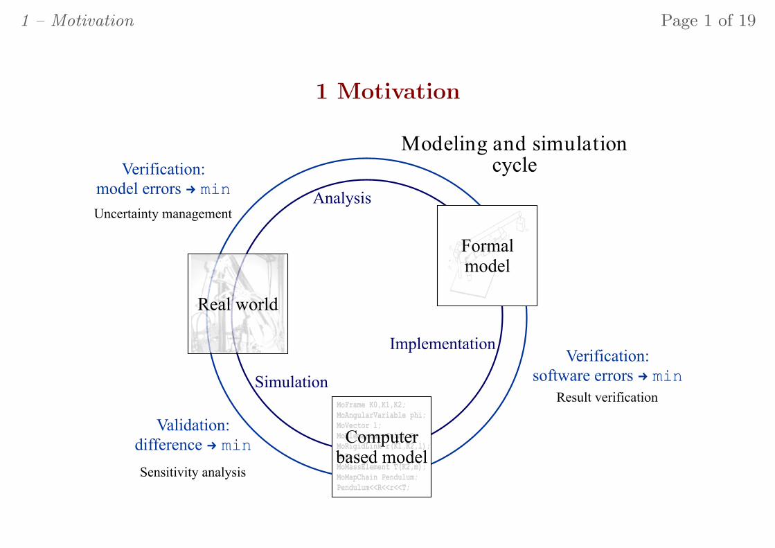
1 Motivation
Implementation
Simulation
Analysis
Real world
Formalmodel
MoFrame K0,K1,K2;
MoAngularVariable phi;
MoVector l;
MoElementaryJoint R;
MoRigidLink r(K1,K2,l);
MoReal m;
MoMassElement T(K2,m);
MoMapChain Pendulum;
Pendulum<<R<<r<<T;
Computerbased model
Verification:
model errors z min
Verification:
software errors z min
Validation:
difference z min
Result verification
Uncertainty management
Sensitivity analysis
Modeling and simulationcycle
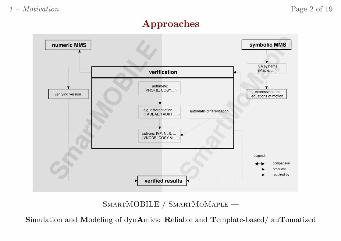
1 – Motivation Page 2 of 19
Approaches
Sm
artM
OB
ILE
Sm
artM
oM
aple
verification
numeric MMS symbolic MMS
CA systems (Maple, ... )
expressions for equations of motion
verifying version
verified results
Legend:
required by
comparison
produces
arithmetic (PROFIL, COSY,...)
alg. differentiation (FADBAD/TADIFF, ...)
solvers: IVP, NLS, ... (VNODE, COSY VI, ...)
automatic differentiation
SmartMOBILE / SmartMoMaple —
Simulation and Modeling of dynAmics: Reliable and Template-based/ auTomatized
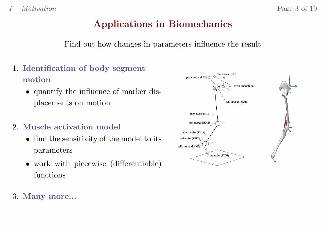
1 – Motivation Page 3 of 19
Applications in Biomechanics
Find out how changes in parameters influence the result
1. Identification of body segment
motion
• quantify the influence of marker dis-
placements on motion
2. Muscle activation model
• find the sensitivity of the model to its
parameters
• work with piecewise (differentiable)
functions
3. Many more...

1 – Motivation Page 4 of 19
Topics
– Theoretical aspects
– Main features of SmartMOBILE and SmartMoMaple
– Identification of body segment motion
– A simplified muscle activation model
– Conclusions
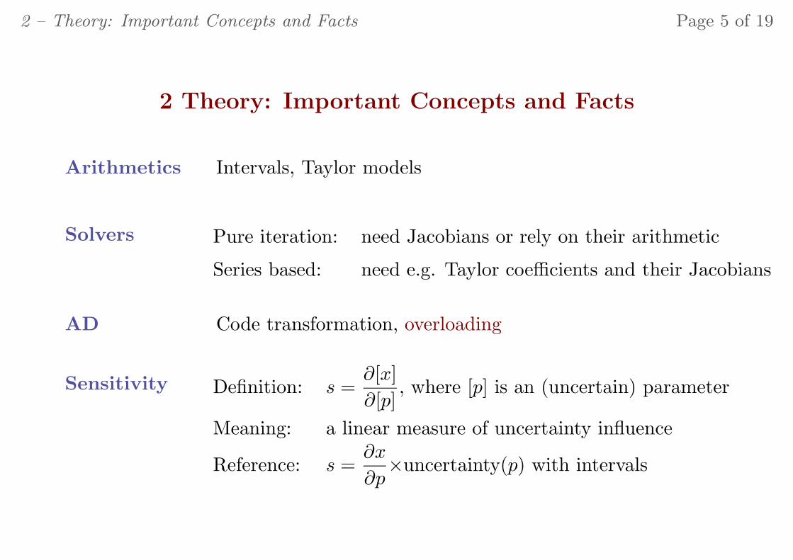
2 – Theory: Important Concepts and Facts Page 5 of 19
2 Theory: Important Concepts and Facts
Arithmetics Intervals, Taylor models
Solvers Pure iteration: need Jacobians or rely on their arithmetic
Series based: need e.g. Taylor coefficients and their Jacobians
AD Code transformation, overloading
Sensitivity Definition: s =∂[x]
∂[p], where [p] is an (uncertain) parameter
Meaning: a linear measure of uncertainty influence
Reference: s =∂x
∂p×uncertainty(p) with intervals
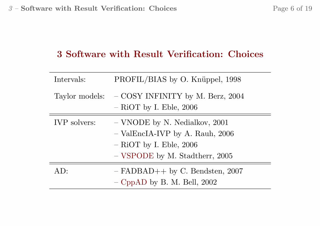
3 – Software with Result Verification: Choices Page 6 of 19
3 Software with Result Verification: Choices
Intervals: PROFIL/BIAS by O. Knuppel, 1998
Taylor models: – COSY INFINITY by M. Berz, 2004
– RiOT by I. Eble, 2006
IVP solvers: – VNODE by N. Nedialkov, 2001
– ValEncIA-IVP by A. Rauh, 2006
– RiOT by I. Eble, 2006
– VSPODE by M. Stadtherr, 2005
AD: – FADBAD++ by C. Bendsten, 2007
– CppAD by B. M. Bell, 2002
4 – Main Features of SmartMOBILE Page 7 of 19
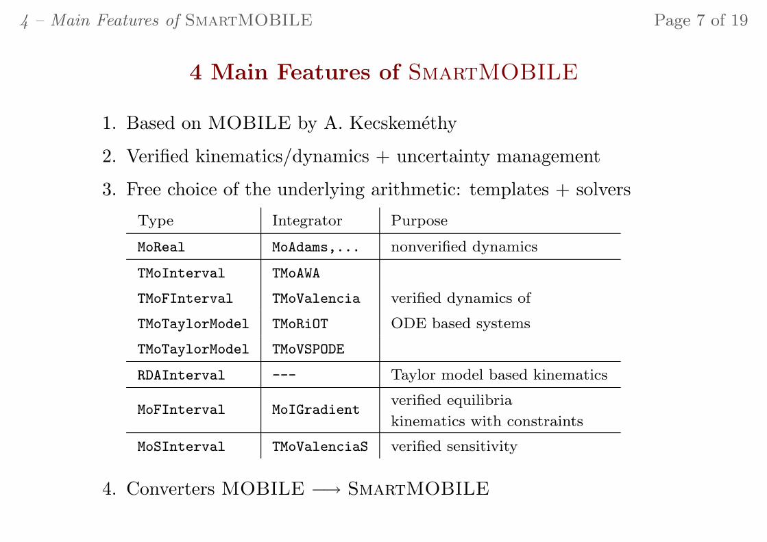
4 Main Features of SmartMOBILE
1. Based on MOBILE by A. Kecskemethy
2. Verified kinematics/dynamics + uncertainty management
3. Free choice of the underlying arithmetic: templates + solvers
Type Integrator Purpose
MoReal MoAdams,... nonverified dynamics
TMoInterval TMoAWA
TMoFInterval TMoValencia verified dynamics of
TMoTaylorModel TMoRiOT ODE based systems
TMoTaylorModel TMoVSPODE
RDAInterval --- Taylor model based kinematics
MoFInterval MoIGradientverified equilibria
kinematics with constraints
MoSInterval TMoValenciaS verified sensitivity
4. Converters MOBILE −→ SmartMOBILE
4 – Main Features of SmartMOBILE Page 8 of 19
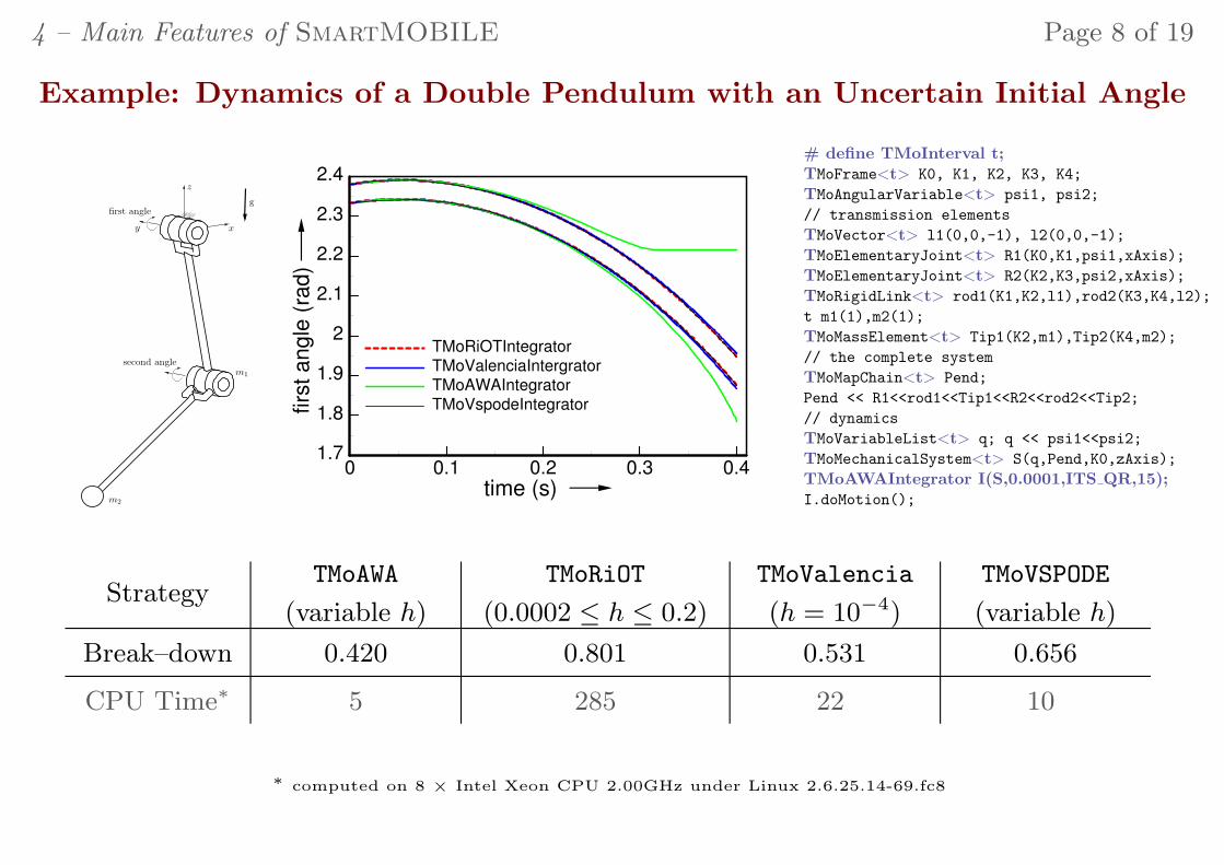
Example: Dynamics of a Double Pendulum with an Uncertain Initial Angle
xy
z
g
m1
m2
first angle
second angle
0 0.1 0.2 0.3 0.4time (s)
1.7
1.8
1.9
2
2.1
2.2
2.3
2.4
firs
t angle
(ra
d)
TMoRiOTIntegrator
TMoValenciaIntergrator
TMoAWAIntegrator
TMoVspodeIntegrator
# define TMoInterval t;TMoFrame<t> K0, K1, K2, K3, K4;
TMoAngularVariable<t> psi1, psi2;
// transmission elements
TMoVector<t> l1(0,0,-1), l2(0,0,-1);
TMoElementaryJoint<t> R1(K0,K1,psi1,xAxis);
TMoElementaryJoint<t> R2(K2,K3,psi2,xAxis);
TMoRigidLink<t> rod1(K1,K2,l1),rod2(K3,K4,l2);
t m1(1),m2(1);
TMoMassElement<t> Tip1(K2,m1),Tip2(K4,m2);
// the complete system
TMoMapChain<t> Pend;
Pend << R1<<rod1<<Tip1<<R2<<rod2<<Tip2;
// dynamics
TMoVariableList<t> q; q << psi1<<psi2;
TMoMechanicalSystem<t> S(q,Pend,K0,zAxis);
TMoAWAIntegrator I(S,0.0001,ITS QR,15);I.doMotion();
StrategyTMoAWA
(variable h)
TMoRiOT
(0.0002 ≤ h ≤ 0.2)
TMoValencia
(h = 10−4)
TMoVSPODE
(variable h)
Break–down 0.420 0.801 0.531 0.656
CPU Time∗ 5 285 22 10
∗ computed on 8 × Intel Xeon CPU 2.00GHz under Linux 2.6.25.14-69.fc8
5 – SmartMoMaple – Symbolic Counterpart to SmartMOBILE Page 9 of 19
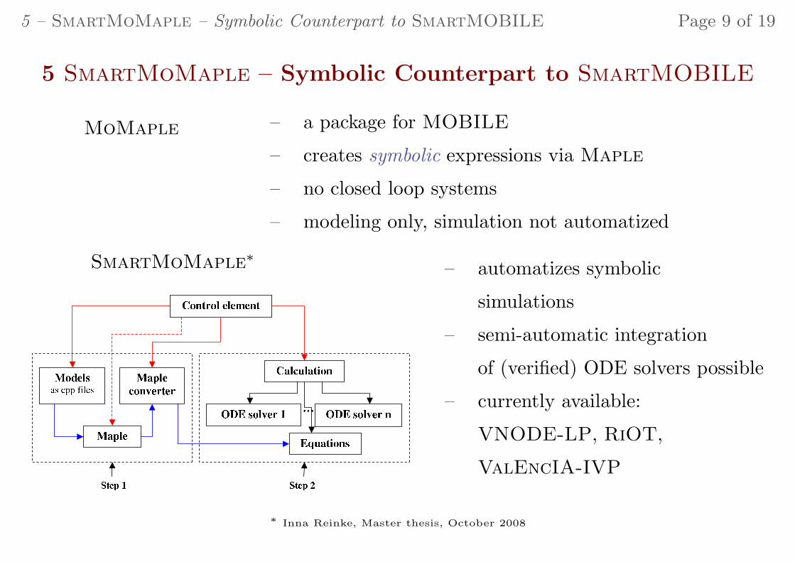
5 SmartMoMaple – Symbolic Counterpart to SmartMOBILE
MoMaple – a package for MOBILE
– creates symbolic expressions via Maple
– no closed loop systems
– modeling only, simulation not automatized
SmartMoMaple∗
– automatizes symbolic
simulations
– semi-automatic integration
of (verified) ODE solvers possible
– currently available:
VNODE-LP, RiOT,
ValEncIA-IVP
∗ Inna Reinke, Master thesis, October 2008
5 – SmartMoMaple – Symbolic Counterpart to SmartMOBILE Page 10 of 19
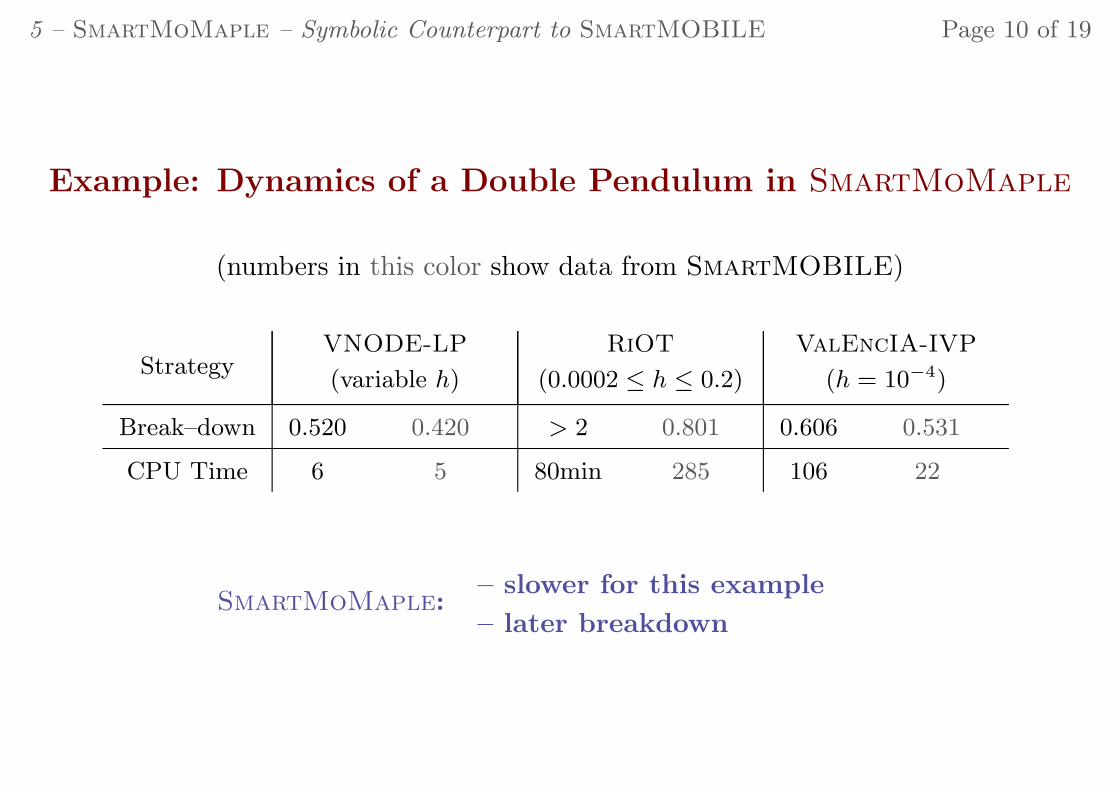
Example: Dynamics of a Double Pendulum in SmartMoMaple
(numbers in this color show data from SmartMOBILE)
StrategyVNODE-LP
(variable h)
RiOT
(0.0002 ≤ h ≤ 0.2)
ValEncIA-IVP
(h = 10−4)
Break–down 0.520 0.420 > 2 0.801 0.606 0.531
CPU Time 6 5 80min 285 106 22
SmartMoMaple:– slower for this example
– later breakdown
6 – Identification of Body Segment Motion Page 11 of 19
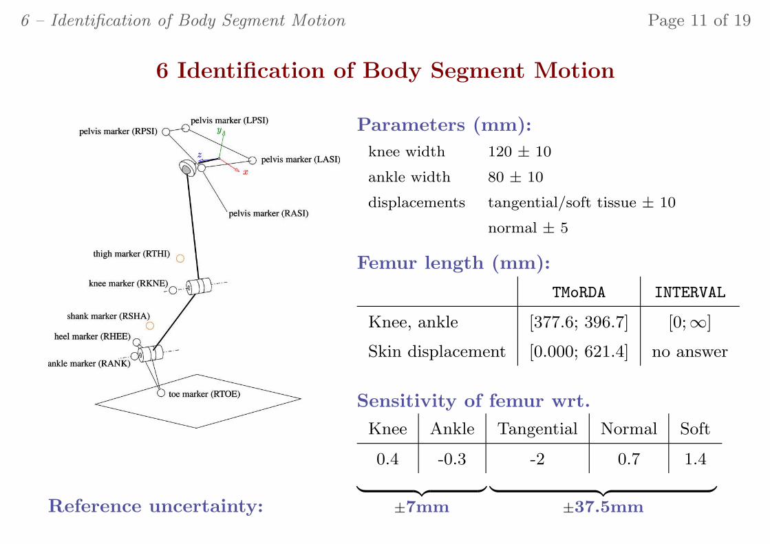
6 Identification of Body Segment Motion
Reference uncertainty:
Parameters (mm):
knee width 120 ± 10
ankle width 80 ± 10
displacements tangential/soft tissue ± 10
normal ± 5
Femur length (mm):
TMoRDA INTERVAL
Knee, ankle [377.6; 396.7] [0;∞]
Skin displacement [0.000; 621.4] no answer
Sensitivity of femur wrt.
Knee Ankle Tangential Normal Soft
0.4 -0.3 -2 0.7 1.4
︸ ︷︷ ︸
±7mm
︸ ︷︷ ︸
±37.5mm
7 – A Simplified Muscle Activation Model Page 12 of 19
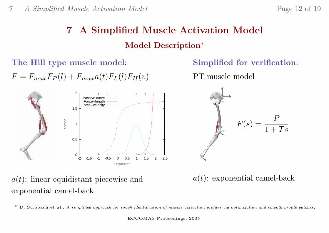
7 A Simplified Muscle Activation Model
Model Description∗
The Hill type muscle model:
F = FmaxFP (l) + Fmaxa(t)FL(l)FH(v)
0
0.5
1
1.5
2
-2 -1.5 -1 -0.5 0 0.5 1 1.5 2 2.5
force
argument
Passive curveForce--length
Force--velocity
a(t): linear equidistant piecewise and
exponential camel-back
Simplified for verification:
PT muscle model
F (s) =P
1 + Ts
a(t): exponential camel-back
∗ D. Strobach et al., A simplified approach for rough identification of muscle activation profiles via optimization and smooth profile patches,
ECCOMAS Proceedings, 2005
7 – A Simplified Muscle Activation Model Page 13 of 19
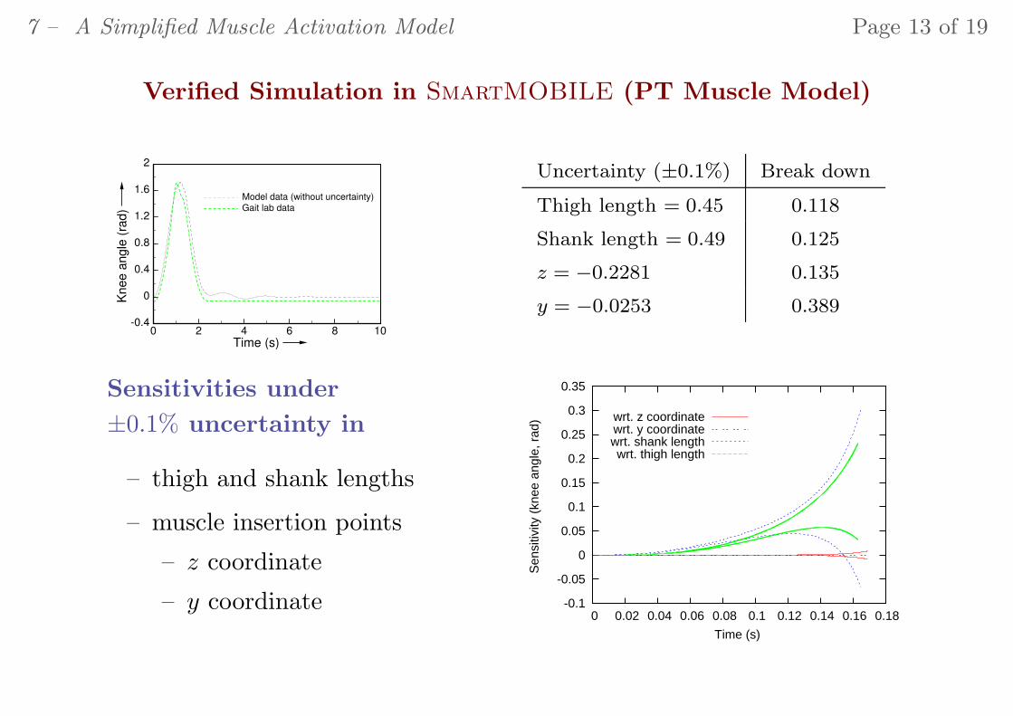
Verified Simulation in SmartMOBILE (PT Muscle Model)
0 2 4 6 8 10 Time (s)
-0.4
0
0.4
0.8
1.2
1.6
2
Kn
ee
an
gle
(ra
d)
Model data (without uncertainty)
Gait lab data
Uncertainty (±0.1%) Break down
Thigh length = 0.45 0.118
Shank length = 0.49 0.125
z = −0.2281 0.135
y = −0.0253 0.389
Sensitivities under
±0.1% uncertainty in
– thigh and shank lengths
– muscle insertion points
– z coordinate
– y coordinate -0.1
-0.05
0
0.05
0.1
0.15
0.2
0.25
0.3
0.35
0 0.02 0.04 0.06 0.08 0.1 0.12 0.14 0.16 0.18
Sen
sitiv
ity (
knee
ang
le, r
ad)
Time (s)
wrt. z coordinatewrt. y coordinatewrt. shank lengthwrt. thigh length
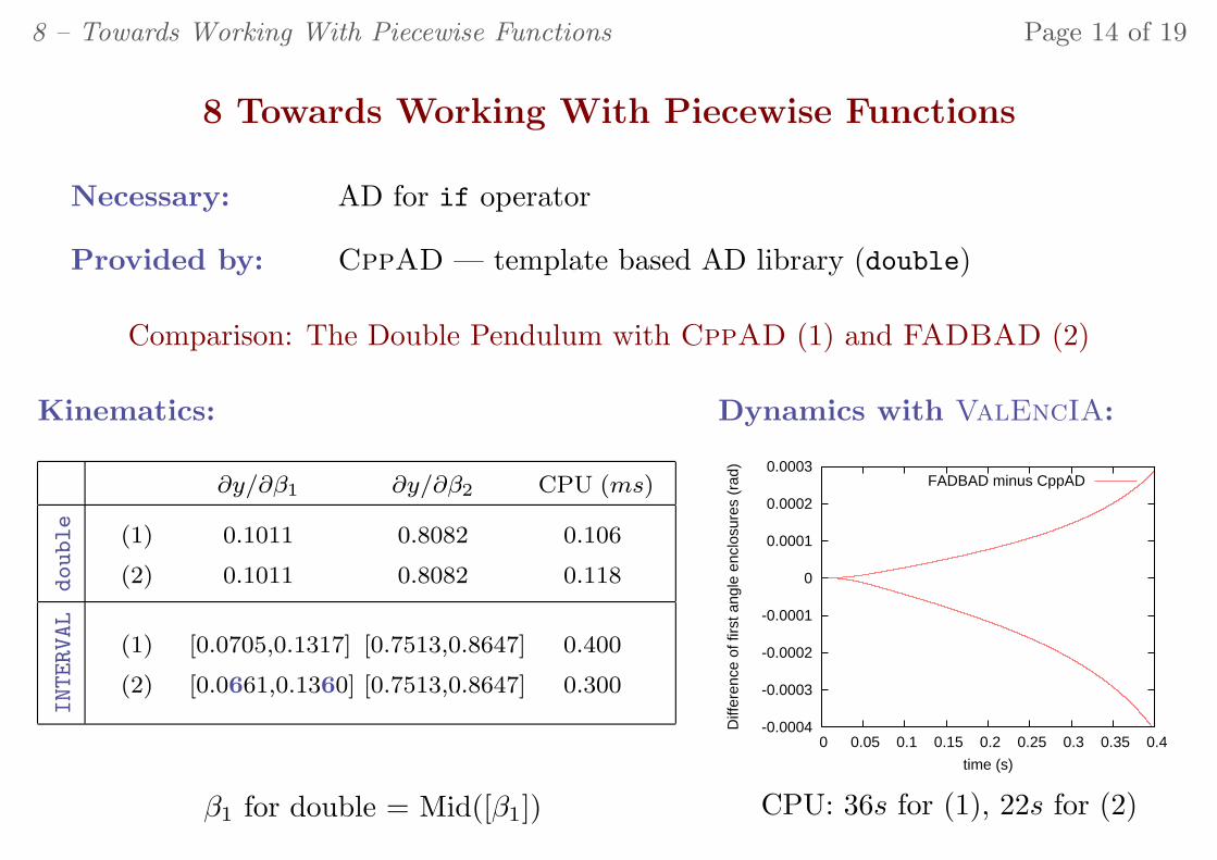
8 – Towards Working With Piecewise Functions Page 14 of 19
8 Towards Working With Piecewise Functions
Necessary: AD for if operator
Provided by: CppAD — template based AD library (double)
Comparison: The Double Pendulum with CppAD (1) and FADBAD (2)
Kinematics:
∂y/∂β1 ∂y/∂β2 CPU (ms)
double
(1) 0.1011 0.8082 0.106
(2) 0.1011 0.8082 0.118
INTERVAL
(1) [0.0705,0.1317] [0.7513,0.8647] 0.400
(2) [0.0661,0.1360] [0.7513,0.8647] 0.300
β1 for double = Mid([β1])
Dynamics with ValEncIA:
-0.0004
-0.0003
-0.0002
-0.0001
0
0.0001
0.0002
0.0003
0 0.05 0.1 0.15 0.2 0.25 0.3 0.35 0.4D
iffer
ence
of f
irst a
ngle
enc
losu
res
(rad
)
time (s)
FADBAD minus CppAD
CPU: 36s for (1), 22s for (2)
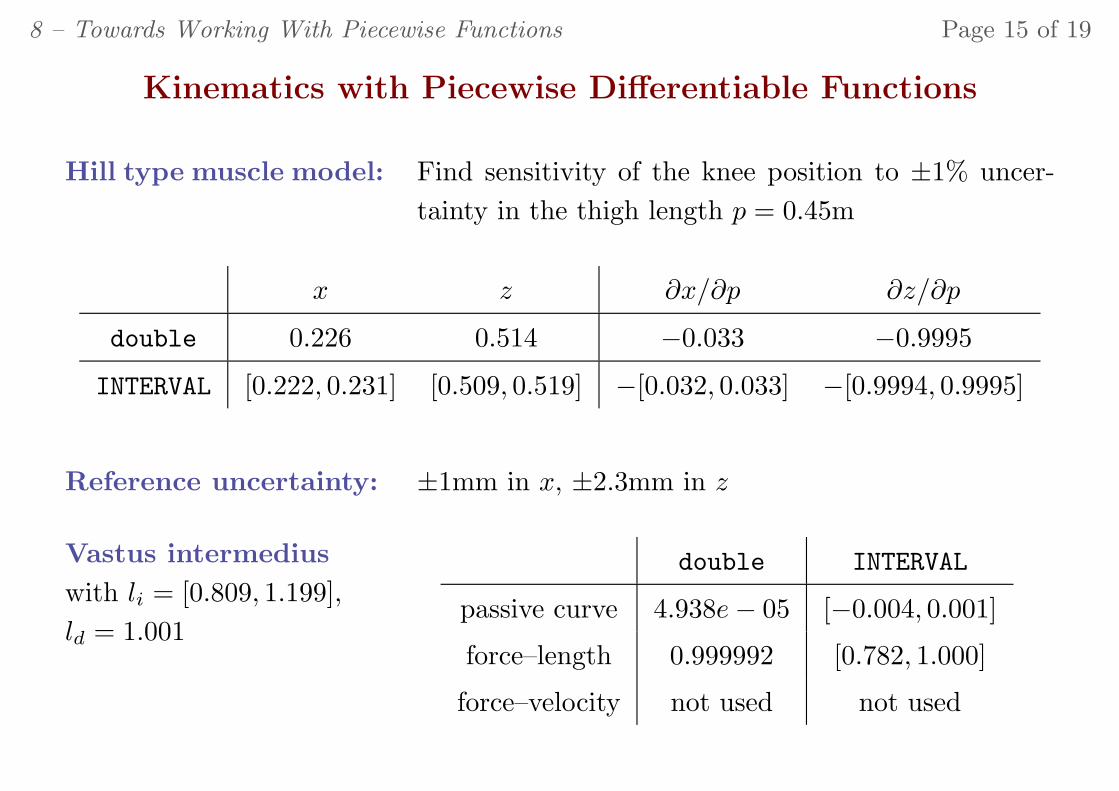
8 – Towards Working With Piecewise Functions Page 15 of 19
Kinematics with Piecewise Differentiable Functions
Hill type muscle model: Find sensitivity of the knee position to ±1% uncer-
tainty in the thigh length p = 0.45m
x z ∂x/∂p ∂z/∂p
double 0.226 0.514 −0.033 −0.9995
INTERVAL [0.222, 0.231] [0.509, 0.519] −[0.032, 0.033] −[0.9994, 0.9995]
Reference uncertainty: ±1mm in x, ±2.3mm in z
Vastus intermedius
with li = [0.809, 1.199],
ld = 1.001
double INTERVAL
passive curve 4.938e − 05 [−0.004, 0.001]
force–length 0.999992 [0.782, 1.000]
force–velocity not used not used
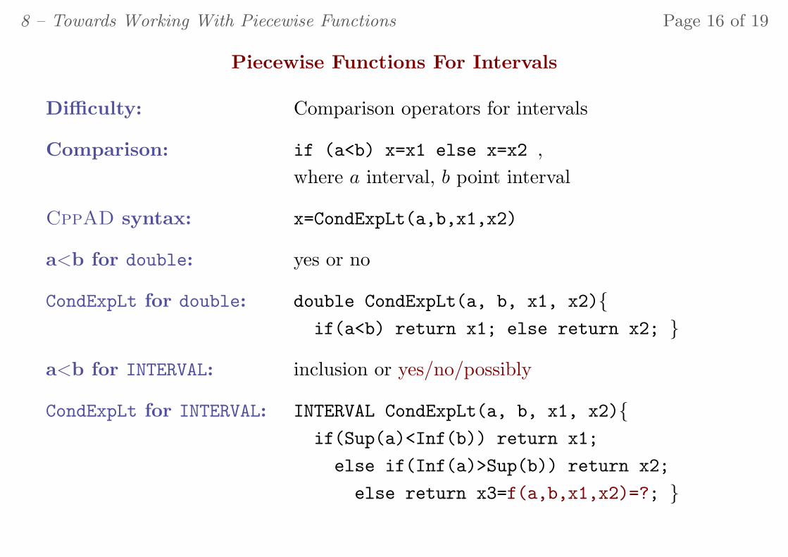
8 – Towards Working With Piecewise Functions Page 16 of 19
Piecewise Functions For Intervals
Difficulty: Comparison operators for intervals
Comparison: if (a<b) x=x1 else x=x2 ,
where a interval, b point interval
CppAD syntax: x=CondExpLt(a,b,x1,x2)
a<b for double: yes or no
CondExpLt for double: double CondExpLt(a, b, x1, x2){
if(a<b) return x1; else return x2; }
a<b for INTERVAL: inclusion or yes/no/possibly
CondExpLt for INTERVAL: INTERVAL CondExpLt(a, b, x1, x2){
if(Sup(a)<Inf(b)) return x1;
else if(Inf(a)>Sup(b)) return x2;
else return x3=f(a,b,x1,x2)=?; }
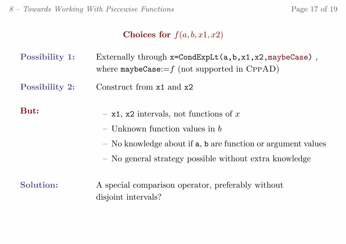
8 – Towards Working With Piecewise Functions Page 17 of 19
Choices for f(a, b, x1, x2)
Possibility 1: Externally through x=CondExpLt(a,b,x1,x2,maybeCase) ,
where maybeCase:=f (not supported in CppAD)
Possibility 2: Construct from x1 and x2
But: – x1, x2 intervals, not functions of x
– Unknown function values in b
– No knowledge about if a, b are function or argument values
– No general strategy possible without extra knowledge
Solution: A special comparison operator, preferably without
disjoint intervals?
8 – Towards Working With Piecewise Functions Page 18 of 19
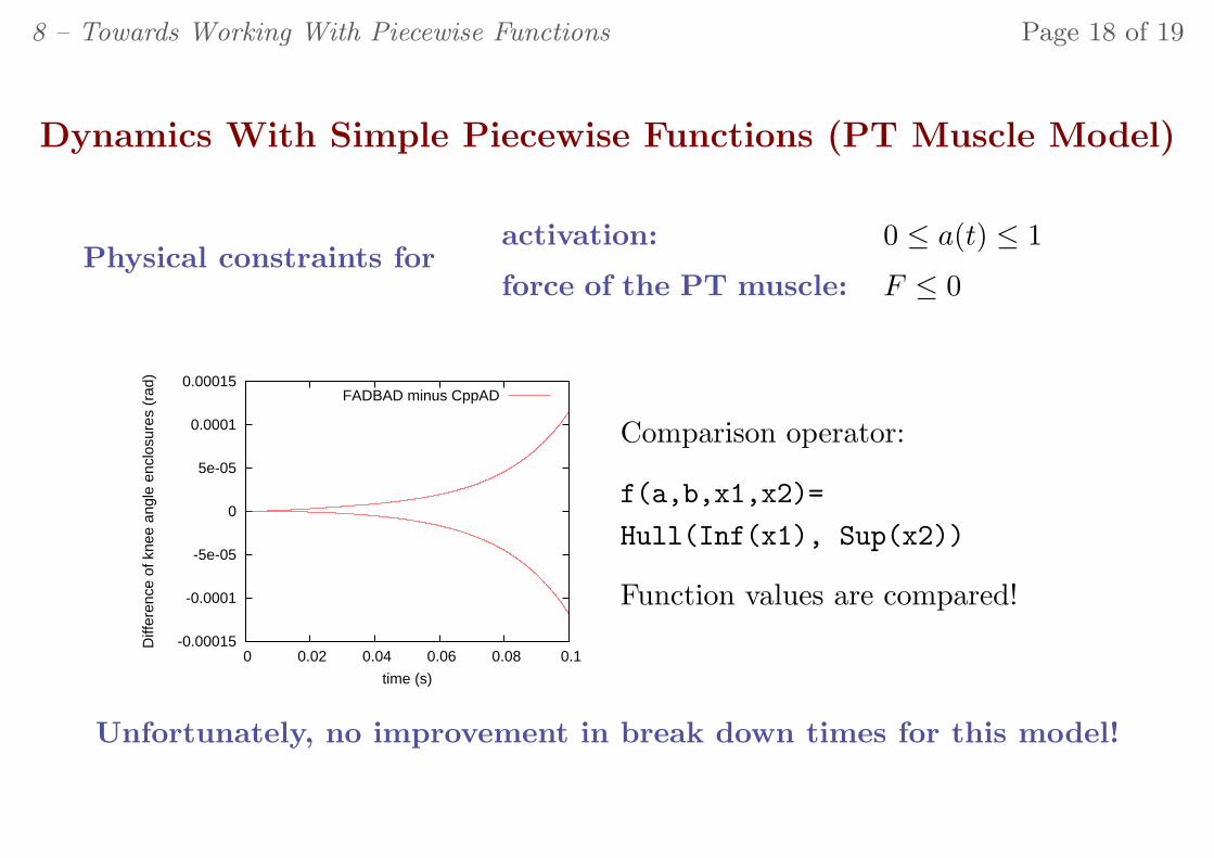
Dynamics With Simple Piecewise Functions (PT Muscle Model)
Physical constraints foractivation: 0 ≤ a(t) ≤ 1
force of the PT muscle: F ≤ 0
-0.00015
-0.0001
-5e-05
0
5e-05
0.0001
0.00015
0 0.02 0.04 0.06 0.08 0.1
Diff
eren
ce o
f kne
e an
gle
encl
osur
es (
rad)
time (s)
FADBAD minus CppAD
Comparison operator:
f(a,b,x1,x2)=
Hull(Inf(x1), Sup(x2))
Function values are compared!
Unfortunately, no improvement in break down times for this model!
9 – Conclusions Page 19 of 19
9 Conclusions
Segment motion: – overestimation reduced through Taylor models
– reference uncertainty is considerable too
Muscle activation: – sensitivities of the smooth model obtained
– simple piecewise functions tested for dynamics
– kinematics for the Hill type muscle model
Open question: definition of if and CondExp for intervals