verifying hierarchical ptolemy ii discrete-event models ... · verifying hierarchical ptolemy ii...

Verifying Hierarchical Ptolemy II Discrete-Event

Models using Real-Time Maude

Kyungmin BaePeter Csaba OlveczkyThomas Huining FengEdward A. LeeStavros Tripakis

Electrical Engineering and Computer SciencesUniversity of California at Berkeley

Technical Report No. UCB/EECS-2010-50

http://www.eecs.berkeley.edu/Pubs/TechRpts/2010/EECS-2010-50.html

May 6, 2010

Copyright © 2010, by the author(s).All rights reserved.

Permission to make digital or hard copies of all or part of this work forpersonal or classroom use is granted without fee provided that copies arenot made or distributed for profit or commercial advantage and that copiesbear this notice and the full citation on the first page. To copy otherwise, torepublish, to post on servers or to redistribute to lists, requires prior specificpermission.

Verifying Hierarchical Ptolemy II Discrete-Event Models using

Real-Time Maude

Kyungmin BaeUniversity of Illinois at Urbana-Champaign

Peter Csaba Olveczky∗

University of Oslo

Thomas Huining Feng, Edward A. Lee, and Stavros TripakisUniversity of California, Berkeley

May 6, 2010

Abstract

This paper defines a real-time rewriting logic semantics for a significant subset of Ptolemy II discrete-event models. This is a challenging task, since such models combine a synchronous fixed-point semanticswith hierarchical structure, explicit time, and a rich expression language. The code generation featuresof Ptolemy II have been leveraged to automatically synthesize a Real-Time Maude verification modelfrom a Ptolemy II design model, and to integrate Real-Time Maude verification of the synthesized modelinto Ptolemy II. This enables a model-engineering process that combines the convenience of Ptolemy IIDE modeling and simulation with formal verification in Real-Time Maude. We illustrate such formalverification of Ptolemy II models with three case studies.

1 Introduction

Model-based design (MBD) [1, 2, 3] emphasizes the construction of high-level models for system design.Useful models are executable, providing simulations of system functionality and/or performance during thedesign phases as a much less costly alternative to building prototypes and testing them. MBD typically raisesthe level of abstraction in system design in general, and for embedded software in particular, from low-levellanguages, such as C++ and Java, to high-level modeling formalisms where concepts like concurrency andtime are first-class notions; this makes it feasible to design systems that would be hard or impossible todesign using low-level methods. Ideally, models are translated (code generated) automatically to producedeployable software. Commercial examples of such modeling and code generation frameworks include Real-Time Workshop (from The MathWorks) and TargetLink (from dSpace), which generate code from Simulinkmodels, LabVIEW Embedded from National Instruments, and SCADE from Esterel Technologies.

Many real-time embedded systems – in areas such as avionics, motor vehicles, and medical systems – aresafety-critical systems, whose failures may cause great damage to persons and/or valuable assets. Modelsof such embedded systems should therefore be formally analyzed to prove safety properties or identifysecurity vulnerabilities. Instead of requiring designers to develop models in some formal framework, apromising approach to formally verify design models is to add formal analysis capabilities to the intuitive,often graphical, informal modeling languages preferred by practitioners by: (i) providing a formal semanticsfor the informal language, (ii) leveraging the code generation features of the informal modeling framework toautomatically translate an informal model to a formal model, and (iii) verifying the synthesized formal model.

For real-time systems, we believe that real-time rewrite theories [4] should be a suitable formalism inwhich to define the semantics of time-based modeling languages, for the following reasons:

∗Corresponding author

1

• Real-time rewrite theories have a natural and “sound” model of timed behavior that makes themsuitable as a semantic framework [4].

• The expressiveness and generality of real-time rewrite theories allow us to give a formal semanticsto languages with advanced functions and data types, new communication models, arbitrary andunbounded data structures, program variables ranging over unbounded domains, and so on.

• The associated Real-Time Maude tool [5] provides a range of formal analysis capabilities, includingsimulation, reachability analysis, and linear temporal logic model checking. Despite the expressivenessof real-time rewriting, timed-bounded LTL properties are often decidable under mild conditions [6].

Real-time rewrite theories and Real-Time Maude have been used to define the formal semantics of – and toprovide a simulator and model checker for – some real-time modeling languages, including: a timed extensionof the Actor model [7], the Orc web services orchestration language [8], a language developed at DoCoMolaboratories for handset applications [9], a behavioral subset of the avionics standard AADL [10], the visualmodel transformation language e-Motions [11], and real-time model transformations in MOMENT2 [12].

Ptolemy II [13] is a well established open-source modeling and simulation tool used in industry. A majorreason for its popularity is Ptolemy II’s powerful yet intuitive graphical modeling language that allows auser to build hierarchical models that combine different models of computations. In this paper, we focuson discrete-event (DE) models; such models are are explicit about the timing behavior of systems, which isan essential feature for the high-level specification of embedded system applications [14, 15]. Discrete-eventmodeling is a time honored and widely used approach for system simulation [16]. More recently, it has beenproposed as basis for synthesis of embedded real-time software [17]. The Ptolemy II DE models have asemantics rooted in the fixed-point semantics of synchronous languages [18].

Like many graphical modeling languages, Ptolemy II DE models lack at present formal verificationcapabilities. Furthermore, Ptolemy II DE models seem to fall outside the class of languages which can begiven an automaton-based semantics, because: (i) certain constructs, such as noninterruptible timers, requirethe use of data structures (such as lists) of unbounded size; (ii) the variables used in, e.g., the transitionsystems in FSM actors range over infinite domains such as the integers; (iii) executing a synchronous steprequires fixed-point computations; and (iv) Ptolemy II has a powerful expression language.

This paper defines a Real-Time Maude semantics for a significant subset of hierarchical Ptolemy II DEmodels. We have used Ptolemy II’s code generation infrastructure to automatically synthesize a Real-TimeMaude verification model from a Ptolemy II model, and have integrated Real-Time Maude verification intoPtolemy II, so that Ptolemy II models can be formally analyzed from within Ptolemy II. We also defineuseful generic temporal logic propositions for such models, so that a Ptolemy II user can easily definehis/her temporal logic requirements without understanding Real-Time Maude or the formal representationof a Ptolemy II model. This integration of Ptolemy II and Real-Time Maude enables a model-engineeringprocess that combines the convenience of Ptolemy II modeling with formal verification in Real-Time Maude.We illustrate such formal verification on three case studies.

Our work on formalizing Ptolemy II is the first attempt to define a Real-Time Maude semantics forsynchronous real-time languages. Apart from the important result of endowing hierarchical Ptolemy II DEmodels with a formal semantics and formal verification capabilities, the main contribution of this work isto show how Real-Time Maude can define the formal semantics of synchronous real-time languages withfixed-point semantics and hierarchical structure.

This paper extends the conference paper [19], that first outlined the Real-Time Maude semantics for flatDE models without general Ptolemy expressions, and the workshop paper [20], that proposed the extensionto hierarchical DE models, by: (i) providing much more detail about our semantics, (ii) explaining howgeneral Ptolemy expressions are handled, and (iii) describing two additional case studies.

The paper is organized as follows. Sections 2 and 3 introduce Real-Time Maude and Ptolemy II DEmodels, respectively. In order to convey the main ideas of our formalization of Ptolemy II DE modelswithout obscuring the presentation with too much detail, we present the semantics in three steps: Section 4defines the Real-Time Maude semantics of flat Ptolemy II DE models where Ptolemy II expressions areconstants; Section 5 extends that semantics to hierarchical DE models; and Section 6 extends it to general

2

Ptolemy II expressions. Section 7 briefly explains how Real-Time Maude verification has been integrated intoPtolemy II and also presents some useful predefined atomic propositions that allow users to easily specifydesired system requirements. Section 8 illustrates Real-Time-Maude-based verification in Ptolemy II withthree case studies. Section 9 discusses related work, and Section 10 gives some concluding remarks. Moredetails about the Real-Time Maude semantics of Ptolemy are given in the longer technical report [21].

2 Real-Time Maude

Real-Time Maude [5] is a language and tool extending Maude [22] to support the formal specification andanalysis of real-time systems. The specification formalism is based on real-time rewrite theories [4]—anextension of rewriting logic [23, 24]—and emphasizes ease and generality of specification.

Real-Time Maude specifications are executable under reasonable assumptions, so that a first form offormal analysis consists of simulating the system’s progress in time by timed rewriting. This can be veryuseful for simulating the system, but any such execution gives us only one behavior among the many possibleconcurrent behaviors of the systems. To gain further assurance about a system one can use model checkingtechniques that explore many different behaviors from a given initial state of the system. Timed search andlinear temporal logic model checking can analyze all possible behaviors from a given initial state (possiblyup to a given duration).

2.1 Preliminaries: Object-Oriented Specification in Maude

Since Real-Time Maude specifications extend Maude specifications, we first recall object-oriented specifica-tion in Maude.

A membership equational logic (Mel) [25] signature is a triple Σ = (K, σ, S), with K a set of kinds,σ = {σw,k}(w,k)∈K∗×K a many-kinded algebraic signature, and S = {Sk}k∈K a K-kinded family of disjointsets of sorts. The kind of a sort s is denoted by [s]. A Mel algebra A contains a set Ak for each kind k,a function Af : Ak1 × · · · × Akn

→ Ak for each operator f ∈ σk1···kn,k, and a subset As ⊆ Ak for each sorts ∈ Sk. TΣ,k and TΣ(X)k denote, respectively, the set of ground Σ-terms with kind k and of Σ-terms withkind over the set X of kinded variables.

A Mel theory is a pair (Σ, E), where Σ is a Mel-signature, and E is a set of conditional equationsof the form (∀X) t = t′ if

∧i pi = qi ∧

∧j wj : sj and conditional memberships of the form (∀X) t :

s if∧

i pi = qi ∧∧

j wj : sj , for t, t′ ∈ TΣ(X)k, s ∈ Sk, the latter stating that t is a term of sort s, providedthe condition holds. Order-sorted notation s1 < s2 can be used to abbreviate the conditional membership(∀x : [s1]) x : s2 if x : s1. Similarly, an operator declaration f : s1 × · · · × sn → s corresponds to declaring fat the kind level and giving the membership axiom (∀x1 : k1, . . . , xn : kn) f(x1, . . . , xn) : s if

∧1≤i≤n xi : si.

The intuitive meaning is that terms in sorts are well-defined, while elements without sorts, such asfact(−5) and fact(3 − 1) in some signature defining the factorial function fact , are either error (or “unde-fined”) values such as fact(−5), or are expressions, such as fact(3 − 1), that are not yet “computed,” butthat will evaluate to well-sorted terms when fully evaluated.

A Maude module specifies a rewrite theory [24, 23] of the form (Σ, E ∪ A,R), where (Σ, E ∪ A) is amembership equational logic theory with A a set of equational axioms such as associativity, commutativity,and identity, so that equational deduction is performed modulo the axioms A. The theory (Σ, E ∪ A)specifies the system’s state space as an algebraic data type. R is a collection of labeled conditional rewriterules specifying the system’s local transitions, each of which has the form1

[l] : t−→ t′ ifm∧

j=1

uj = vj ,

1In general, the condition of such rules may not only contain equations uj = vj , but also rewrites wi −→ w′i and memberships

tk : sk; however, the specification in this paper does not use this extra generality.

3

where l is a label. Intuitively, such a rule specifies a one-step transition from a substitution instance of t tothe corresponding substitution instance of t′, provided the condition holds; that is, the substitution instancesof the equalities uj = vj follow from E ∪ A. The rules are implicitly universally quantified by the variablesappearing in the Σ-terms t, t′, uj , and vj . The rules are applied modulo the equations E ∪A.2

We briefly summarize the syntax of Maude. Operators are introduced with the op keyword: op f :s1 . . . sn -> s. They can have user-definable syntax, with underbars ‘_’ marking the argument positions,and are declared with the sorts of their arguments and the sort of their result. Some operators can haveequational attributes, such as assoc, comm, and id, stating, for example, that the operator is associativeand commutative and has a certain identity element. Such attributes are then used by the Maude engine tomatch terms modulo the declared axioms. An operator can also be declared to be a constructor (ctor) thatdefines the carrier of a sort. There are three kinds of logical statements, namely, equations—introduced withthe keywords eq, or, for conditional equations, ceq—memberships—declaring that a term has a certain sortand introduced with the keywords mb and cmb—and rewrite rules—introduced with the keywords rl andcrl. The mathematical variables in such statements are either explicitly declared with the keywords var andvars, or can be introduced on the fly in a statement without being declared previously, in which case theymust be have the form var:sort. We will make frequent use of the fact that an equation f(t1, . . . , tn) = twith the owise (for “otherwise”) attribute can be applied to a subterm f(. . .) only if no other equation withleft-hand side f(u1, . . . , un) can be applied.3 Finally, a comment is preceded by ‘***’ or ‘---’ and lasts tillthe end of the line.

In Maude, kinds are not explicitly declared; instead the kind of a sort s is denoted [s]. Maude alsosupports the declaration of partial functions using the arrow ‘~>’:

op f : s1 ... sn ~> s .

The above declaration is equivalent to the kinded declaration

op f : [s1] ... [sn] -> [s] .

In object-oriented Maude modules one can declare classes and subclasses. A class declaration

class C | att1 : s1, ... , attn : sn

declares an object class C with attributes att1 to attn of sorts s1 to sn. An object of class C in a given stateis represented as a term

< O : C | att1 : val1, ..., attn : valn >

of the built-in sort Object, where O is the object’s name or identifier, and where val1 to valn are the currentvalues of the attributes att1 to attn and have sorts s1 to sn. Objects can interact with each other in avariety of ways, including the sending of messages. A message is a term of the built-in sort Msg, where thedeclaration

msg m : p1 . . . pn -> Msg

defines the syntax of the message (m) and the sorts (p1 . . . pn) of its parameters. In a concurrent object-oriented system, the state, which is usually called a configuration, is a term of the built-in sort Configuration.It has the structure of a multiset made up of objects and messages. Multiset union for configurations is de-noted by a juxtaposition operator (empty syntax) that is declared associative and commutative and havingthe none multiset as its identity element, so that order and parentheses do not matter, and so that rewritingis multiset rewriting supported directly in Maude. The dynamic behavior of object systems is axiomatizedby specifying each of its concurrent transition patterns by a rewrite rule. For example, the configurationfragment on the left-hand side of the rule

2Operationally, a term is reduced to its E-normal form modulo A before any rewrite rule is applied in Maude. Under thecoherence assumption [26] this is a complete strategy to achieve the effect of rewriting in E ∪A-equivalence classes.

3A specification with owise equations can be transformed to an equivalent system without such equations [22].

4

rl [l] : m(O,w) < O : C | a1 : x, a2 : y, a3 : z > =>

< O : C | a1 : x + w, a2 : y, a3 : z > m’(y,x)

contains a message m, with parameters O and w, and an object O of class C. The message m(O,w) does notoccur in the right-hand side of this rule, and can be considered to have been removed from the state by therule. Likewise, the message m’(y,x) only occurs in the configuration on the right-hand side of the rule, andis thus generated by the rule. The above rule, therefore, defines a parametrized family of transitions (one foreach substitution instance) in which a message m(O,w) is read and consumed by an object O of class C, withthe effect of altering the attribute a1 of the object and of sending a new message m’(y,x). By convention,attributes, such as a3 in our example, whose values do not change and do not affect the next state of otherattributes need not be mentioned in a rule or an equation. Attributes like a2 whose values influence thenext state of other attributes or the values in messages, but are themselves unchanged, may be omitted fromright-hand sides of rules/equations.

A subclass inherits all the attributes, equations, and rules of its superclasses4, and multiple inheritanceis supported.

2.2 Object-Oriented Specification in Real-Time Maude

A Real-Time Maude timed module specifies a real-time rewrite theory [4], that is, a rewrite theory R =(Σ, E ∪A,R), such that:

1. (Σ, E ∪ A) contains an equational subtheory (ΣTIME , ETIME) ⊆ (Σ, E ∪ A), satisfying the TIMEaxioms in [4], which specifies a sort Time as the time domain (which may be discrete or dense).Although a timed module is parametric on the time domain, Real-Time Maude provides some prede-fined modules specifying useful time domains. For example, the modules NAT-TIME-DOMAIN-WITH-INFand POSRAT-TIME-DOMAIN-WITH-INF define the time domain to be, respectively, the natural num-bers and the nonnegative rational numbers, and contain the subsort declarations Nat < Time andPosRat < Time. These modules also add a supersort TimeInf, which extends the sort Time with an“infinity” value INF.

2. The sort of the “states” of the system has the designated sort System.

3. The rules in R are decomposed into:

• “ordinary” rewrite rules that model instantaneous change, and• tick (rewrite) rules that model the elapse of time in a system. Such tick rules have the form

l : {t}−→ {t′} if cond, where t and t′ are of sort System, { } is a built-in constructor of a newsort GlobalSystem, and where we have associated to such a rule a term u of sort Time denotingthe duration of the rewrite. In Real-Time Maude, tick rules, together with their durations, arespecified with the syntax

crl [l] : {t} => {t′} in time u if cond .

The initial state of a real-time system so specified must be reducible to a term {t0}, for t0 a ground termof sort System, using the equations in the specification. The form of the tick rules then ensures uniform timeelapse in all parts of a system.

2.3 Formal Analysis in Real-Time Maude

We summarize below the Real-Time Maude analysis commands. All Real-Time Maude analysis commandsand their semantics are explained in [5].

Real-Time Maude’s timed fair rewrite command simulates one behavior of the system up to a certainduration. It is written with syntax

4The attributes, equations, and rules of a class cannot be redefined by its subclasses, but subclasses may introduce additionalattributes, equations, and rules.

5

(tfrew t in time <= timeLimit .)

where t is the term to be rewritten (“the initial state”), and timeLimit is a ground term of sort Time.Real-Time Maude provides a variety of search and model checking commands for further analyzing timed

modules by exploring all possible behaviors—up to a given number of rewrite steps, duration, or satisfactionof other conditions—that can be nondeterministically reached from the initial state. For example, Real-TimeMaude extends Maude’s search command—which uses a breadth-first strategy to search for states that arereachable from the initial state and match the search pattern and satisfy the search condition—to search forstates that can be reached within a given time interval from the initial state.

Finally, Real-Time Maude extends Maude’s linear temporal logic model checker to check whether eachbehavior (possibly “up to a certain time,” as explained in [5]) satisfies a temporal logic formula. Statepropositions, possibly parametrized, should be declared as operators of sort Prop, and their semantics shouldbe given by (possibly conditional) equations of the form

{statePattern} |= prop = b

for b a term of sort Bool, which defines the state proposition prop to hold in all states {t} such that {t}|= prop evaluates to true. A temporal logic formula is constructed by state and clocked5 propositions andtemporal logic operators such as True, False, ~ (negation), /\, \/, -> (implication), [] (“always”), <>(“eventually”), U (“until”), and W (“weak until”). The command

(mc t |=u formula .)

is the model checking command which checks whether the temporal logic formula formula holds in allbehaviors starting from the initial state t.

3 Ptolemy II and its DE Model of Computation

The Ptolemy project6 studies modeling, simulation, and design of concurrent, real-time, embedded systems.Ptolemy II is a modeling environment that supports multiple modeling paradigms, which we call models ofcomputations (MoCs), that govern the interaction between concurrent components.

Modeling with heterogeneous MoCs [13] is a key research area of the Ptolemy project. The supportedMoCs include FSM (finite state machine), dataflow, and DE (discrete events). Such MoCs can compose tocreate heterogeneous models with well-defined semantics.

3.1 Discrete-Event Models

A Ptolemy II model consists of a set of actors, each having a set of ports that can be connected. An outputport outputs data. An input port receives data from the output port that it is connected to.

A composition of actors, including the interconnections between their ports, can be encapsulated as anactor in its own right, which may also have input and output ports. Such an actor obtained by compositionis called a composite actor. An input port of a composite actor can be connected to input ports of the actorsinside, which means that external inputs are transferred to those inner actors. Similarly, an output port ofa composite actor can be connected to output ports of the actors inside. An actor that is not composite iscalled an atomic actor.

The focus of this paper is the formalization of Ptolemy II discrete-event (DE) models. In DE, the datasent and received at actors’ ports are events. Each event has two components: a tag and a value. Accordingto the tagged signal model [27], a tag t is a pair (τ, n) ∈ R≥0 × N, where τ is the timestamp denoting themodel time at which the event occurs, and n is the microstep index. Microstep indices are useful for modeling

5A clocked proposition involves both the state and the duration of the path leading to the state (the system “clock”), asexplained in [5].

6http://ptolemy.org/

6

http://ptolemy.org/

Q := empty; // Initialize the global event queue to be empty.

for each actor A do

A.init(); // Initialize actor A, and possibly generate initial events, stored in Q.

end for;

while Q is non-empty do

E := set of all simultaneous events at the head of Q;

remove E from Q;

initialize ports with values in E or "unknown";

while port values changed do

for each actor A do

A.fire(); // May change port values

end for;

end while; // Fixed-point reached for the current tag

for each actor A do

A.postfire(); // Updates actor state, and may generate new queue events

end for;

end while;

Figure 1: Pseudo-code of Ptolemy II DE semantics.

multiple events with identical timestamps happening in sequence, where earlier events may cause later ones.Tags are totally ordered using a lexicographical order: (τ1, n1) ≤ (τ2, n2) if and only if τ1 < τ2, or τ1 = τ2

and n1 ≤ n2. Two events are simultaneous if they have identical tags.The operational semantics of DE in Ptolemy II can be explained with the pseudo-code in Figure 1. An

event queue is used for the execution. Events in the event queue are ordered by their tags. Initially, theevent queue is empty. At the beginning of the execution, all actors are initialized, and some actors may postinitial events to the event queue. Operation then proceeds by iterations. In each iteration, the events withthe smallest tag are extracted from the event queue and presented to the actors that receive them. Thoseactors are fired, which means they are invoked to process their input events, and they may also output eventsthrough their output ports. A difference between the DE MoC in Ptolemy II and standard DE simulatorsis that the former incorporates a synchronous-reactive semantics for processing simultaneous events [18].When events are extracted from the event queue for the receiving actors to process, the semantics for thatiteration is defined as the least fixed-point of the output values, in a way similar to a synchronous model [28].Concretely, the outputs are first set to a predefined value called unknown. Then, the actors receiving eventsare fired in an arbitrary order, possibly repeatedly, until a fixed-point of all output values is reached. Thisallows Ptolemy II models to have feedback loops. If the model contains causality cycles, the fixed-point mayhave ports with value unknown. Finally, when the fixed-points for the port values have been found, the actorsthat have received input or have been fed events are executed, in the sense that their states are updated andthat they may generate future events that are inserted into the event queue (postfire).

3.2 Atomic Actors

We briefly introduce a subset of the Ptolemy II atomic actors whose semantics has been formalized in Real-Time Maude. Their semantics is defined in terms of the actions init, fire, and postfire. (We ignore otheractions, such as prefire and finalize, which are not important in this paper.)

• Clock. Ptolemy’s clock actors have as parameters a clock period, and same-sized arrays values andoffsets. In each period, a clock generates events with given values and offsets within the period. Forexample, if the period is 5, the values are {3, 8}, and the offsets are {2, 4}, then an event with value 3is generated at times 2, 7, 12, 17, 22, . . . , and an event with value 8 is generated at times 4, 9, 14, . . . .That is, the init action posts an event to the event queue with timestamp 0 for itself to process; the

7

fire action is triggered by that event and sends the value to the output port; and the postfire actionposts the next event to the event queue, with timestamp equal to the beginning of the next period.

• Current Time. Ptolemy’s current time actor produces an output token on each firing with a valuethat is the current model time. That is, the init and postfire actions do nothing, and the fire actionconsumes an input event, and outputs an event whose timestamp and value are both equal to thetimestamp of the input event.

• Pulse. When an input is received, a pulse actor outputs pulses with values given by the values param-eter; the parameter indexes specifies when those values should be produced. A zero is produced whenthe iteration count does not match an index. For example, if the indexes parameter is “{1, 3, 0, 2,4}”, and the values are stored in array A, then the output in the first 5 invocation of fire is A[1], A[3],A[0], A[2], and A[4]. After that, the output is always 0, unless yet another parameter, repeat, is setto true, in which case the output is repeated. The init action does nothing, fire outputs a value, andpostfire updates the number of times fire has been invoked.

• Time Delay. A timed delay actor propagates an incoming event after a given delay, which is given bythe delay parameter. If the delay parameter is 0.0, then there is a ”microstep” delay in the generationof the output event.

• Variable Delay. A variable delay actor works in a similar way as a timed delay actor, except that theamount of time delay is specified by an incoming token through the delay port.

• Timer. The difference between a timer actor and a delay actor is that the value of the generatedoutput of a timer is not the same as the input, but is given by the output parameter of this actor. Thelength of the delay is specified by the input received in the actor’s lone input port.

• Noninterruptible Timer. A noninterruptible timer is similar to a normal timer, but with the differencethat the noninterruptible timer actor delays the processing of a new input if it has not finished pro-cessing a previous input. That is, while an input event is being delayed and the corresponding outputhas not been sent, other input events are queued.

• Timed Plotter. A timed plotter records its received events and the times they were received.

• (Atomic) Finite State Machine (FSM) Actor. A finite state machine (FSM) actor is a transitionsystem containing a finite set of states (or “locations”), a finite set of “variables,” and a finite set oftransitions. A transition has a guard expression, and can contain a set of output actions. Outputactions may assign values to the variables belonging to the FSM actor and/or may send values to theoutput ports of the actor. When an FSM actor is fired, there is never more than one enabled transition.If there is exactly one enabled transition then it is chosen and the actions contained by the transitionare executed. Under the DE director, only one transition step is performed in each iteration.

3.3 Composite Actors

An essential feature of Ptolemy II is hierarchy. It helps hide internal details of parts of a model. It istherefore crucial for managing model complexity, and for achieving modularity and scalability.

Ptolemy II hierarchical models contain components (or actors) that are themselves Ptolemy II models.Such a hierarchical model can again be encapsulated and be seen as a single composite actor. An inner actorof a DE composite actor is executed if that inner actor receives some events at its input ports or if it is fedan event from the event queue. Figure 2 illustrates a hierarchical composition of actors.

In Ptolemy II, each composite actor can have its own director, that is, model of computation, to supportheterogeneous modeling. If the director of a composite actor is the same as the director of the parent actor,it is called a transparent actor. In this paper, we consider only transparent cases since we verify DE models.

8

A0 A3 A4

A5A2

A7A1 A6

Figure 2: A hierarchical composition of actors. A0–A7 are actors, A0 and A3 are composite actors, trianglesare ports, and dashed lines are connections.

3.4 Modal Models

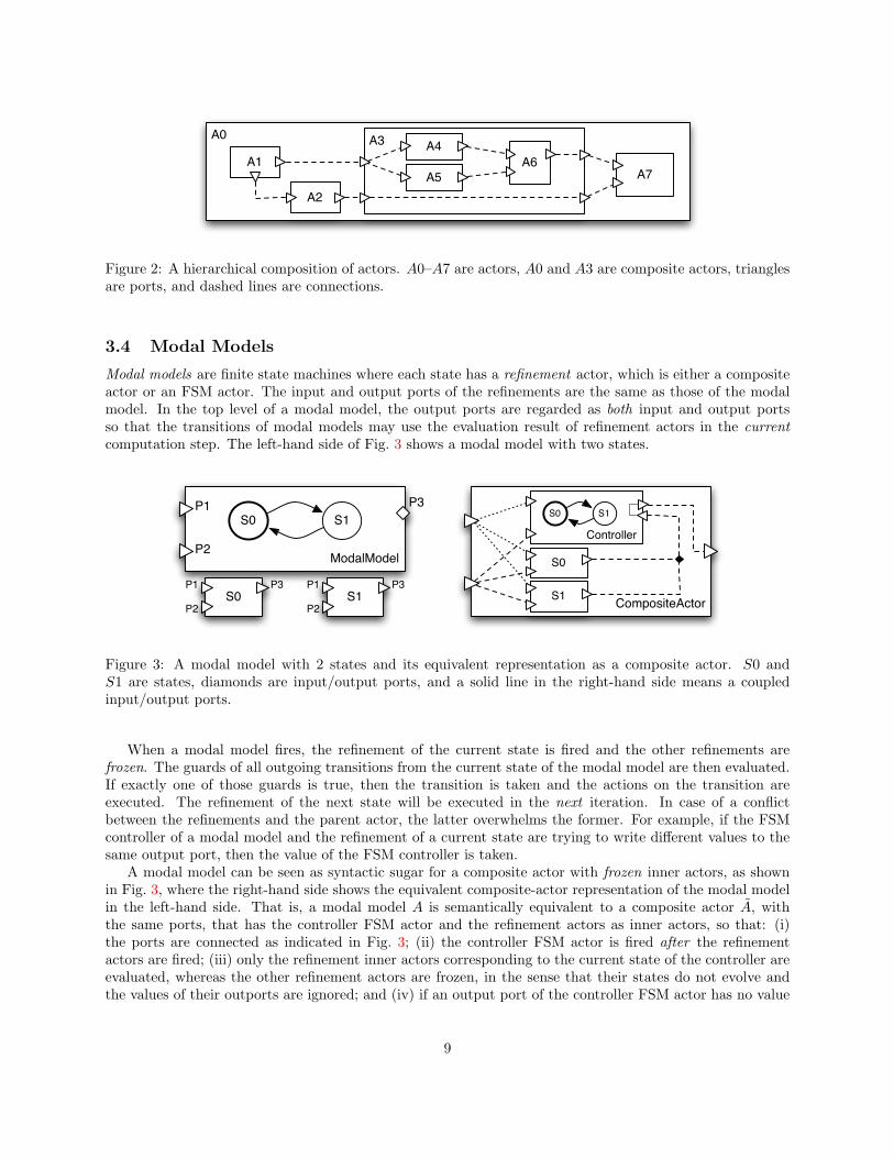
Modal models are finite state machines where each state has a refinement actor, which is either a compositeactor or an FSM actor. The input and output ports of the refinements are the same as those of the modalmodel. In the top level of a modal model, the output ports are regarded as both input and output portsso that the transitions of modal models may use the evaluation result of refinement actors in the currentcomputation step. The left-hand side of Fig. 3 shows a modal model with two states.

ModalModel

P1

P2

P3S0 S1

S0P1

P2

P3S1

P1

P2

P3

CompositeActor

S0

S1

Controller

S0 S1

Figure 3: A modal model with 2 states and its equivalent representation as a composite actor. S0 andS1 are states, diamonds are input/output ports, and a solid line in the right-hand side means a coupledinput/output ports.

When a modal model fires, the refinement of the current state is fired and the other refinements arefrozen. The guards of all outgoing transitions from the current state of the modal model are then evaluated.If exactly one of those guards is true, then the transition is taken and the actions on the transition areexecuted. The refinement of the next state will be executed in the next iteration. In case of a conflictbetween the refinements and the parent actor, the latter overwhelms the former. For example, if the FSMcontroller of a modal model and the refinement of a current state are trying to write different values to thesame output port, then the value of the FSM controller is taken.

A modal model can be seen as syntactic sugar for a composite actor with frozen inner actors, as shownin Fig. 3, where the right-hand side shows the equivalent composite-actor representation of the modal modelin the left-hand side. That is, a modal model A is semantically equivalent to a composite actor A, withthe same ports, that has the controller FSM actor and the refinement actors as inner actors, so that: (i)the ports are connected as indicated in Fig. 3; (ii) the controller FSM actor is fired after the refinementactors are fired; (iii) only the refinement inner actors corresponding to the current state of the controller areevaluated, whereas the other refinement actors are frozen, in the sense that their states do not evolve andthe values of their outports are ignored; and (iv) if an output port of the controller FSM actor has no value

9

but its coupled input port has some value, then the output port will have the same value as the input port.

3.5 Subset of Ptolemy II with Real-Time Maude Semantics

We currently support Real-Time Maude analysis of transparent discrete event (DE) Ptolemy II modelsconstructed by the following actors: composite actors, modal models, finite state machine (FSM), timed delay,variable delay, clock, current time, timer, noninterruptible timer, pulse, ramp, timed plotter, set variable,expression, single event actors, and algebraic actors such as add/subtract, const, and scale. We also supportconnections with multiple destinations, split signals, and both single ports and multi-input ports.

3.6 Code Generation Infrastructure

Ptolemy II is built in a highly modular manner, with flexible and extensible components that communicatethrough generic interfaces. This type of inter-component communication introduces overhead, however,which generally results in component models that are slower than custom-built code. To regain efficiency,Ptolemy II offers a code generation capability with which inter-component communication is reduced bygenerating “monolithic” code with highly specialized components.

The code generation framework uses an adapter-based mechanism. A codegen adapter is a componentthat generates code for an actor. Each actor may have multiple associated adapters, one for each targetlanguage (such as C and VHDL). An adapter essentially consists of a Java class file and a code template filethat together specify the actor’s behavior. The latter contains code blocks written in the target language.Supplied with a set of adapters and an initial model, the code generation framework examines the modelstructure and invokes the adapters to harvest code blocks from the code template files. The main advantagesof this scheme are, first, that it decouples the writing of Java code and target code (otherwise the targetcode would be wrapped in strings and be interspersed with Java code), and second, that it allows using atarget language specific editor while working on the target language code blocks.

3.7 Example: A Simple Traffic Light System

Figure 4 shows a Ptolemy DE model of a simple traffic light system consisting of one car light and onepedestrian light at a pedestrian crossing. Each light is represented by a set of set variable actors (Pred andPgrn represent the pedestrian light, and Cred, Cyel, and Cgrn represent the car light). A light is on iff thecorresponding variable has the value 1. The lights are controlled by two finite state machine (FSM) actors,CarLight and PedestrianLight, that send values to set the variables; in addition, CarLight sends signals(that are delayed by one time unit) to the PedestrianLight actor through its Pgo and Pstop output ports.

Figure 4: A simple traffic light model in Ptolemy II.

Figure 5a shows the FSM actor PedestrianLight. This actor has three input ports (Pstop, Pgo, andSec), two output ports (Pgrn and Pred), three internal states, and three transitions. This actor reacts to

10

signals from the car light (by way of the delay actors) by turning the pedestrian lights on and off. Forexample, if the actor is in local state Pred and receives input through its Pgo port, then it goes to statePgreen, outputs the value 0 through its Pred port, and outputs the value 1 through its Pgrn port.

Figure 5b shows the FSM actor CarLight. Assuming that the clock actor sends a signal every time unit,we notice, e.g., that one time unit after both the red and yellow car lights are on, these are turned off andthe green car light is turned on by sending the appropriate values to the variables (output: Cred = 0; Cyel

= 0; Cgrn = 1). The car light then stays green for two time units before turning yellow.

(a) PedestrianLight (b) CarLight

Figure 5: The FSM actors for pedestrian lights and car lights.

4 Real-Time Maude Semantics of Flat Ptolemy II DE Models

To convey our ideas underlying the Real-Time Maude formalization of the semantics of Ptolemy II DE modelswithout introducing too many details, this section presents a slightly simplified version of our semantics, inthat we present a semantics for

1. flat Ptolemy models; that is, models without hierarchical actors, and

2. assume that all Ptolemy II expressions are defined by constants and simple arithmetic and comparisonoperations.

Section 5 shows how this slightly simplified semantics is extended to hierarchical models, and Section 6shows how we deal with general Ptolemy expressions that include variables. The entire executable Real-Time Maude semantics is available at http://www.ifi.uio.no/RealTimeMaude/Ptolemy.

4.1 Representing Flat Ptolemy II DE Models in Real-Time Maude

This section explains how a flat Ptolemy II DE model is represented as a Real-Time Maude term in (theslightly simplified version of) our semantics. We only show the representation for a subset of the atomicactors in Ptolemy II DE models, and refer to [21] for the definition of the other actors.

Our Real-Time Maude semantics is defined in an object-oriented style, where the global state has theform of a multiset

{actors connections < global : EventQueue | queue : event queue >}

where

11

http://www.ifi.uio.no/RealTimeMaude/Ptolemy

• actors are objects corresponding to the actor instances in the Ptolemy model,

• connections are the connections between the ports of the different actors, and

• < global : EventQueue | queue : event queue > is an object whose queue attribute denotes theglobal event queue.

This section explains the representation of these entities in Real-Time Maude, and Section 4.2 definesthe semantics of the behaviors of the Ptolemy II models.

4.1.1 Actors

Each Ptolemy II actor is modeled in Real-Time Maude as an object instance of a subclass of the followingclass Actor:

class Actor | ports : Configuration, parameters : Configuration .

The ports attribute denotes the set of ports of the actor. The parameters attribute represents the pa-rameters of the actor, together with their user-defined values/expressions. In our model, both ports andparameters are modeled as objects. In particular, a parameter is represented as an object, with a name (theidentifier of the parameter object) and one attribute value:

sorts ParamId . subsort Qid < ParamId < Oid . --- names for parameters

class Parameter | value : Value .

This simple parameter model will be extended in Section 6 when we consider a parameters whose values areexpressions that may include variables.

Some actors, such as clocks and timed plotters, have an internal clock measuring “model time.” Suchactors are represented as object instances of subclasses of the following class TimeActor, where currentTimedenotes the current model time:

class TimeActor | currentTime : Time . subclass TimeActor < Actor .

Clocks As explained above, the Ptolemy parameters of an actor (period, offsets, and values for clock actors)are represented in the parameters attribute. The only additional attribute needed for the Real-Time Mauderepresentation of clock actors is the attribute index keeping track of the “index” of the offsets and valuesarrays for the next event to be generated:

class Clock | index : Nat . subclass Clock < Actor .

For instance, the initial state of the clock described above is represented by the object7

< ’Clock : Clock | index : 0,

parameters : < ’period : Parameter | value : # 5 >

< ’offsets : Parameter | value : {# 2.0, # 4.0} >

< ’values : Parameter | value : {# 3, # 8} >,

ports : < ’output : OutPort | value : # 0, status : absent >

< ’trigger : InPort | value : # 0, status : absent >

< ’period : InPort | value : # 0, status : absent > >

Current Time Since the superclass TimeActor already contains the current time in the currentTimeattribute, the CurrentTime subclass does not add any new attributes:

class CurrentTime . subclass CurrentTime < TimeActor .

7See Section 4.1.2 for the representation of ports.

12

Timed Plotter A timed plotter records its received data values and the times they were received. Inour representation, these values are recorded as a list (source: s1 time: t1 value: v1) ++ ... ++(source: sn time: tn value: vn) of triples (source: si time: ti value: vi), denoting, respectively,the port from which the data was received, the time it was received, and the received data value. Since suchan actor must keep track of the currentTime, the TimedPlotter class is a subclass of TimeActor:

class TimedPlotter | eventHistory : EventHistory . subclass TimedPlotter < TimeActor .

sort EventTriple EventHistory .

subsort EventTriple < EventHistory .

op source:_time:_value:_ : EPortId Time Value -> EventTriple [ctor] .

op emptyHistory : -> EventHistory [ctor] .

op _++_ : EventHistory EventHistory -> EventHistory [ctor assoc id: emptyHistory] .

Other Actors Since the actor parameters are represented in the parameters attribute of the superclassActor, most actors do not add any new attributes to the attributes inherited from Actor. The pulse actoradds an attribute index that keeps track of the iteration count:

class Delay . --- timed delay

class VariableDelay .

class Timer .

class Pulse | index : Nat .

subclass Delay VariableDelay Timer Pulse < Actor .

A noninterruptible timer needs some attributes to keep track of the state: processing is true when thetimer has not finished processing previous inputs. The waitQueue is a list that stores (the values of) theinputs received while the timer is “busy.” This list is therefore a list of time values declared in the usualMaude style. The Real-Time Maude declaration of this class is

class NonInterruptibleTimer | processing : Bool, waitQueue : TimeList .

subclass NonInterruptibleTimer < Actor .

sort TimeList . subsort Time < TimeList .

op emptyList : -> TimeList [ctor] .

op __ : TimeList TimeList -> TimeList [ctor assoc id: emptyList] .

Finite State Machine (FSM) Actors An FSM-Actor is characterized by its current state, its transitions,and its local variables (the latter are represented by parameters):

class FSM-Actor | currState : Location, initState : Location, transitions : TransitionSet .

subclass FSM-Actor < Actor .

A location is the sort of the local “states” of the transition system. In particular, quoted identifiers (Qids)are state names:

sort Location . subsorts Qid < Location .

We model the set of transitions as a semi-colon-separated set of transitions of the forms1 --> s2 {guard: g output: pi1 |-> ei′1

;...; pik |-> ei′k

set: vj1 |-> ej′1;...; vil |-> ej′

l}

for states/locations s1 and s2, port names pi, variables vi, and expressions ei. The guard, output, and/orset parts may be omitted. In Real-Time Maude, such sets of transitions are declared as follows:

13

sorts Transition TransitionSet . subsort Transition < TransitionSet .

op _-->_‘{_‘} : Location Location TransBody -> Transition [ctor] .

op emptyTransitionSet : -> TransitionSet [ctor] .

op _;_ : TransitionSet TransitionSet -> TransitionSet [ctor assoc comm id: emptyTransitionSet] .

sort TransBody .

op guard:_output:_set:_ : Exp AssignMap AssignMap -> TransBody [ctor] .

In the flat setting, we assume that all expressions consist of

• constants (which have sort Value) : (0, 1, true, . . . )

• variables (which are represented by parameter objects)

• simple arithmetic, logical, and comparison operators: +, ×, &&, !, <, . . . .

• isPresent(P ), which is true if there is some (current) input in the given port P, and is false if thereis no current input in port P.

4.1.2 Ports

A port is represented as an object, with a name (the identifier of the port object), a status (unknown,present, or absent, denoting the “current” knowledge about whether there is input/output in the currentiteration), and a value. We also have subclasses for input and output ports:

sorts PortId . subsort Qid < PortId < Oid . --- names for (local) ports

class Port | status : PortStatus, value : Value .

class InPort . subclass InPort < Port .

class OutPort . subclass OutPort < Port .

sort PortStatus .

ops unknown present absent : -> PortStatus [ctor] .

We also support multiple input ports, which are connected to multiple output ports:

class MultiInPort | source : EPortIdSet . subclass MultiInPort < InPort .

4.1.3 Connections

A connection is a term po ==> pi1 ; . . . ; pinof sort Connection, where the pjs are either local port names or

have the form a!p for a the relative name of an actor. Such a connection connects the output port po to allthe input ports pi1 , . . . , pin . Since connections appear in configurations, and are not messages, they are alsoterms of sort ObjectConfiguration:

sort Connection .

op _==>_ : EPortId EPortIdSet -> Connection [ctor] .

subsort Connection < ObjectConfiguration .

sort EPortId .

op _!_ : ActorID PortId -> EPortId [ctor] .

sort EPortIdSet . subsort EPortId < EPortIdSet .

op noPort : -> EPortIdSet [ctor] .

op _;_ : EPortIdSet EPortIdSet -> EPortIdSet [ctor assoc comm id: noPort] .

14

A multiple input port and its connection are transformed to a set of input ports with duplicated connec-tions, whose port names are annotated by the name of their source ports as follows:

var PORTS : Configuration . vars P P’ : PortId . var PS : PortStatus . var EPIS EPIS’ : EPortIdSet .

vars O O’ : Oid . var V : Value .

eq < O : Actor | ports : PORTS >

(O’ ! P’ ==> (O ! P) ; EPIS)

=

< O : Actor | ports : 

 PORTS >

(O’ ! P’ ==> (O ! P # (O’ ! P’) ) ; (O ! P) ; EPIS) .

eq < O : Actor | ports : PORTS >

(O’ ! P’ ==> (O ! P) ; EPIS)

= < O : Actor | ports : PORTS > (O’ ! P’ ==> EPIS) .

4.1.4 The Global Event Queue

The global event queue is represented by an object

< global : EventQueue | eventQueue : event queue >

where event queue is an ::-separated list, ordered according to time until firing, of terms of the form

set of events ; time to fire ; microstep

where the set of events is a set of events, with each event characterized by the “global port name” wherethe generated event should be output and the corresponding value, time to fire denotes the time until theevents are supposed to fire, and microstep is the additional “microstep” until the event fires:

sort Event .

op event : EPortId Value -> Event [ctor] .

sort Events . subsort Event < Events .

op noEvent : -> Events [ctor] .

op __ : Events Events -> Events [ctor assoc comm id: noEvent] .

sort TimedEvent .

op _;_;_ : Events Time Nat -> TimedEvent [ctor] .

sort EventQueue . subsort TimedEvent < EventQueue .

op nil : -> EventQueue [ctor] .

op _::_ : EventQueue EventQueue -> EventQueue [ctor assoc id: nil] .

4.1.5 Example: Representing the Flat Traffic Light Model

Consider the flat non-fault-tolerant traffic light system given in Section 3.7. The Real-Time Maude repre-sentation of the TimedDelay2 delay actor in the initial state is then

< ’TimedDelay2 : Delay | parameters : < ’delay : Parameter | value : # 1.0 >,

ports : < ’input : InPort | value : # 0, status : absent >

< ’output : OutPort | value : # 0, status : absent > >

Likewise, the FSM actor CarLightNormal is represented as the term8

8To save space, some terms are replaced by ‘...’

15

< ’CarLightNormal : FSM-Actor |

initState : ’Cinit, currState : ’Cinit,

parameters : < ’count : Parameter | value : # 1 >,

ports : < ’Sec : InPort | value : # 0, status : absent >

< ’Pgo : OutPort | value : # 0, status : absent >

...,

transitions :

(’Cinit --> ’Cred

{guard: (# true)

output: (’Cred |-> # 1) ; (’Cyel |-> # 0) ; (’Cgrn |-> # 0)

set: ’count |-> # 0}) ;

(’Cred --> ’Cred

{guard: (isPresent(’Sec) && (’count lessThan # 2))

output: emptyMap set: ’count |-> (’count + # 1)}) ; ... >

The connection from the output port output of the Clock actor to the input port Sec of CarLightNormaland the input port Sec of PedestrianLightNormal is represented by the term

(’Clock ! ’output) ==> (’PedestrianLightNormal ! ’Sec) ; (’CarLightNormal ! ’Sec)

The entire state thus consists of two FSM actor objects, ten connections, two delay objects, five setvariable objects, and the global event queue object.

4.2 Specifying the Behavior of Flat DE Models

The behavior of Ptolemy DE models can be summarized as repeatedly performing the following actions:

• Advance time until the time when the first event(s) in the event queue should fire.

• Then an iteration of the system is performed. That is,

1. The events that are supposed to fire are added to the corresponding output ports; the status ofall other ports is set to unknown.

2. (Fire) Then the fixed point of all ports is computed by gradually increasing the knowledge aboutthe presence/absence of inputs to and output from ports until a fixed-point is reached.

3. (Postfire) Finally, the actors with inputs or scheduled events are executed; states are changed andnew events are generated and inserted into the global event queue.

The following tick rule advances time until the time when the first events in the event queue are scheduled;that is, until the time-to-fire of the first events in the event queue is 0 (we first declare all the variables usedin this section):

var CF : Configuration . vars NECF NECF’ : NEConfiguration .

vars SYSTEM OBJECTS REST PORTS PORTS2 PARAMS : ObjectConfiguration . vars OBJ OBJECT : Object .

vars O O’ : Oid. vars P P : PortId . var PS : PortStatus . vars EPIS EPIS : EPortIdSet .

var VI : VarId . vars V V1 V2 TV : Value. vars E TG : Exp .

var EVTS : Events . var QUEUE : EventQueue . var EH : EventHistory .

var T T’ : Time . var NZT : NzTime . var N : Nat . var NZ : NzNat . vars STATE STATE’ : Location .

var TRANSSET : TransitionSet . var BODY : TransBody . vars OL AL : AssignMap .

rl [tick] :

{SYSTEM < global : EventQueue | queue : (EVTS ; NZT ; N) :: QUEUE >}

=>

{delta(SYSTEM, NZT)

< global : EventQueue | queue : (EVTS ; 0 ; N) :: delta(QUEUE, NZT) >}

in time NZT .

16

In this rule, the first element in the event queue has non-zero delay NZT. Time is advanced by this amountNZT, and as a consequence, the (first component of the) event timer goes to zero. In addition, the functiondelta is applied to all the other objects (denoted by SYSTEM) in the system. The function delta definesthe effect of time elapse on the objects. This function is also applied to the other elements in the eventqueue, where it decreases the remaining time of each event set by the elapsed time NZT (x monus y equalsmax(0, x− y)):

op delta : EventQueue Time -> EventQueue .

eq delta((EVTS ; T ; N) :: QUEUE, T’) = (EVTS ; T monus T’ ; N) :: delta(QUEUE, T’) .

eq delta(nil, T) = nil .

The function delta on configurations distributes over the elements in the configuration, and must bedefined on the single objects which are instance of TimeActor, as shown later.

op delta : Configuration Time -> Configuration .

eq delta(none, T) = none .

eq delta(NECF NECF’, T) = delta(NECF, T) delta(NECF’, T) .

The next rule is a “microstep tick rule” that advances “time” with some microsteps if needed to enablethe first events in the event queue:

rl [shortTick] :

{SYSTEM < global : EventQueue | queue : (EVTS ; 0 ; NZ ) :: QUEUE >}

=>

{SYSTEM < global : EventQueue | queue : (EVTS ; 0 ; 0 ) :: QUEUE >} .

Finally, when the remaining time and microsteps of the first events in the event queue are both zero, aniteration of the system can be performed:

rl [executeStep] :

{SYSTEM < global : EventQueue | queue : (EVTS ; 0 ; 0) :: QUEUE >}

=>

{< global : EventQueue | queue : QUEUE >

postfire(portFixPoints(addEventsToPorts(EVTS, clearPorts(SYSTEM))))} .

The function clearPorts starts the execution of an iteration by clearing all ports; that is, it sets the statusof each port in the system to unknown. The operator addEventsToPorts inserts the events scheduled to fireinto the corresponding output ports. The portFixPoints function then finds the fixed points for all theport (this function corresponds to the fire action in Ptolemy), and postfire “executes” the steps on thecomputed port fixed-points by changing the states of the objects and generating new events and insertingthem into the global event queue.

It is important to notice that these functions are declared to be partial functions. Since the equationsdefining these functions only apply to terms of sort Configuration and its subsorts (NEConfiguration,ObjectConfiguration, and so on), this ensures that clearPorts has been computed before addEventsToPortsis computed, which again must happen before portFixPoints is computed, and so on. Mathematically, thismeans that our equations are confluent.

ops clearPorts portFixPoints postfire : Configuration ~> Configuration .

To completely define the behavior of the actors, we must define the functions clearPorts, portFixPoints,postfire, and delta on the different objects in the system.

17

4.2.1 Clearing Ports

The clearPorts function distributes to each actor object in the state, and then clears all the ports of eachactor, that is, sets the status to unknown (notice, as mentioned above, that the equations only apply toterms of sort Configuration):

eq clearPorts(OBJ CF) = clearPorts(OBJ) clearPorts(CF) .

eq clearPorts(< O : Actor | ports : PORTS >) = < O : Actor | ports : clearPorts(PORTS) > .

eq clearPorts( PORTS) = clearPorts(PORTS) .

eq clearPorts(CF) = CF [owise] .

4.2.2 Computing the Fixed-Point for Ports

The idea behind the definition of the function portFixPoints, that computes the fixed-point for the valuesof all the ports, is simple. The state has the form portFixPoints(objects and connections), where initially,the only port information are the events scheduled for this iteration. For each possible case when the statusof an unknown port can be determined to be either present or absent, there is an equation

eq portFixPoints(< O : ... | ports : PORTS, ... >

connections and other objects) =

portFixPoints(< O : ... | ports : PORTS, ... >

connections and other objects) .

(and similarly for deciding that input/output will be absent). The fixed-point is reached when no suchequation can be applied. Then, the portFixPoints operator is removed by using the owise construct ofReal-Time Maude:

eq portFixPoints(OBJECTS) = OBJECTS [owise] .

We first define the general cases of portFixPoints that apply to any Actor instance. The followingequation propagates port status from a “known” output port to a connecting unknown input port. Thepresent/absent status (and possibly the value) of the output port P of actor O is propagated to the inputport P’ of the actor O’ through the connection (O ! P) ==> ((O’ ! P’) ; EPIS):

ceq portFixPoints(< O : Actor | ports : PORTS >

((O ! P) ==> ((O’ ! P’) ; EPIS))

< O’ : Actor | ports : < P’ : InPort | status : unknown > PORTS2 >

REST)

= portFixPoints(< O : Actor | >

((O ! P) ==> ((O’ ! P’) ; EPIS))

< O’ : Actor | ports : < P’ : InPort | status : PS, value : V > PORTS2 >

REST)

if PS =/= unknown .

If all input ports of an actor are absent, then the actor should not generate any output, unless it has ascheduled event from the event queue. In this case, the status of each output port of the actor is set toabsent:

ceq portFixPoints(< O : Actor | ports : PORTS > REST)

= portFixPoints(< O : Actor | ports : 

setUnknownOutPortsAbsent(PORTS) > REST)

if allInputPortsAbsent(PORTS) .

op allInputPortsAbsent : Configuration -> Bool .

eq allInputPortsAbsent( PORTS)

18

= (PS == absent) and allInputPortsAbsent(PORTS) .

eq allInputPortsAbsent(PORTS) = true [owise] .

op setUnknownOutPortsAbsent : Configuration ~> Configuration .

eq setUnknownOutPortsAbsent( PORTS)

= setUnknownOutPortsAbsent(PORTS) .

eq setUnknownOutPortsAbsent(PORTS) = PORTS [owise] .

It is also possible that some actor has an isolated input port that has no incoming connection. Obviously,the input port has no value; i.e., its status should be absent:

ceq portFixPoints(< O : Actor | ports : PORTS > REST)

= portFixPoints(< O : Actor | ports : PORTS > REST)

if not connectedInPort(O ! P, REST) .

op connectedInPort : EPortId Configuration -> Bool .

eq connectedInPort(O ! P, (O’ ! P’ ==> (O ! P) ; EPIS) < O’ : Actor | > CF) = true .

eq connectedInPort(O ! P, CF) = false [owise] .

The portFixPoints function must then be defined for each kind of actor to decide whether the actorproduces any output in a given port. For example, the timed delay actor does not produce any output inthis iteration as a result of any input. Therefore, if its status is unknown (that is, the delay actor did notschedule an event for this iteration), its output port should be set to absent:

eq portFixPoints(< O : Delay | ports : PORTS > REST)

= portFixPoints(< O : Delay | ports : PORTS > REST) .

Actors, such as variable delay, clock actors, timers, etc., that generate “delayed” events as a result of receivinginput, have the same definition of portFixPoint.

Other actors generate immediate output when receiving input. For example, when the current time actorgets an input, it outputs the current model time, given by its currentTime attribute. Furthermore, whenits lone input port is absent, its lone output port is also set to absent:

ceq portFixPoints(< O : CurrentTime | currentTime : T,

ports : 

< P’ : OutPort | status : unknown > >

REST)

= portFixPoints(< O : CurrentTime | ports : 

< P’ : OutPort | status : PS , value : # T >

REST)

if PS =/= unknown .

Likewise, when a pulse actor gets input through its trigger port, it should generate immediate outputthrough its output port. Then an output value is produced as described in Section 3.2, which is done by thefunction getValue:

eq portFixPoints(< O : Pulse | index : N,

parameters : < ’indexes : Parameter | value : V1 >

< ’values : Parameter | value : V2 > PARAMS,

ports : < ’trigger : InPort | status : present >

< ’output : OutPort | status : unknown > PORTS >

REST)

= portFixPoints(< O : Pulse | ports : < ’trigger : InPort | >

< ’output : OutPort | status : present,

value : getValue(V1, V2, N) >

PORTS >

REST) .

19

For FSM actors, the portFixPoints function must check whether at most one transition is enabled atany time by evaluating the guard expressions. In the following equation, one transition from the currentstate STATE is enabled, and there is no other enabled transition. In addition, there is some input to theactor (through input port P’), and some output ports have status unknown. The function updateOutPortsthen updates the status and the values of the output ports according to the current state and input:

ceq portFixPoints(< O : FSM-Actor | ports : < P’ : InPort | status : present >

 PORTS,

currState : STATE, parameters : PARAMS,

transitions : (STATE --> STATE’ {guard: TG output: OL set: AL}) ;

TRANSSET >

REST)

=

portFixPoints(< O : FSM-Actor | ports : < P’ : InPort | >

updateOutPorts(PARAMS, OL, PORTS) >

REST)

if transApplicable(< P’ : InPort | > PORTS, PARAMS, TG)

/\ noGuardTrue(< P’ : InPort | > PORTS, PARAMS, TRANSSET) .

The function transApplicable holds if the guard evaluates to true, for the current values of the local statevariables (as given by the parameters objects) and current knowledge of port states and values. Likewise,noGuardTrue holds iff no transition in the transitions set given as last argument starts in the given locationand satisfies the guard. The definition of these functions is straight-forward and is not shown here.

The updateOutPorts function is defined as follows. Each output port is assigned a value of the corre-sponding output action of the given transition, and all remaining output ports are set to be absent in theend of the update process:

op updateOutPorts : Configuration AssignMap Configuration -> Configuration .

eq updateOutPorts(PARAMS, (VI |-> V ; OL), < VI : OutPort | status : unknown > PORTS)

= < VI : OutPort | status : present, value : V > updateOutPorts(PARAMS, OL, PORTS) .

eq updateOutPorts(PARAMS, OL, PORTS) = setUnknownOutPortsAbsent(PORTS) [owise] .

Other equations for portFixPoints on FSM actors specify the cases when no transition is enabled. Inthese cases, every output ports should be set to absent :

ceq portFixPoints(< O : FSM-Actor | ports : PORTS,

parameters : PARAMS, transitions : TRANSSET >

REST)

=

portFixPoints(< O : FSM-Actor | ports : setUnknownOutPortsAbsent(PORTS) >

REST)

if allGuardsFalse( PORTS, PARAMS, TRANSSET) .

The function setUnknownOutPortsAbsent sets the status of each output port with status unknown toabsent, and the function allGuardsFalse checks whether the guard in each transition evaluates to falsein the current environment.

4.2.3 Postfire

The postfire function updates internal states and generates future events that are inserted into the eventqueue. The postfire function distributes over the actor objects in the configuration:

eq postfire(OBJECT NECF) = postfire(OBJECT) postfire(NECF) .

eq postfire(CF) = CF [owise] .

20

The second equation defines the “default” case when postfire does not change the state of an actorand does not generate a new event. Therefore, we only to define the positive cases where either the internalstate of an actor should be changed as a result of the firing, and/or when when the actor generates a futureevent that should be inserted into the event queue. For example, the current time actor does not have astate that is changed, except by the passage of time, and does not schedule later events, so that we do notneed to specify an equation defining postfire for current time objects.

Sometimes, postfire generates a new event with value v that should fire at time t and microstep n fromthe current time. In these cases, postfire puts the new event into the event queue, and the correspondingequation has the form

eq postfire(< O : C | ports : PORTS, ... >)

< global : EventQueue | queue : QUEUE >

=

< O : C | ... >

< global : EventQueue | queue : addEvent(event(O ! P, v), t, n, QUEUE) > .

where the function addEvent inserts the new event in the correct place in the event queue.

Delay If a time delay actor has input in its ’input port, then it generates an event with delay equal tothe current value of the ’delay parameter. If this delay is 0.0, the microstep is 1, otherwise the microstepis 0:

eq postfire(< O : Delay | ports : < ’input : InPort | status : present, value : V >

< ’output : OutPort | >,

parameters : < ’delay : Parameter | value : TV > PARAMS >)


=

< O : Delay | >)

< global : EventQueue | queue : addEvent(event(O ! ’output, V), toTime(TV),

if toTime(TV) == 0 then 1 else 0 fi, QUEUE) > .

The variable delay actor has an extra delay port to specify time delay. If the delay port is absent, thebehavior is the same as the delay actor. However, if the delay port has some value, the value of the port isused instead of the ’delay parameter:

eq postfire(< O : VariableDelay | ports : < ’input : InPort | status : present, value : V >

< ’delay : InPort | status : present, value : TV >

< ’output : OutPort | > PORTS >)

= < O : VariableDelay | >



Clock When a clock actor produces output, the postfire function should schedule the next event, andupdate the index variable (in the second equation a new “cycle” is started):

ceq postfire(< O : Clock | ports : PORTS,

parameters : < ’offsets : Parameter | value : V1 >

< ’values : Parameter | value : V2 > PARAMS,

index : N >)


=

< O : Clock | index : N + 1 >

< global : EventQueue | queue : addEvent(event(O ! P, V2(#(s N))), TIME-TO-FIRE,

if TIME-TO-FIRE == 0 then 1 else 0 fi, QUEUE) >

if TIME-TO-FIRE := toTime((V1(#(s N))) - (V1(# N)))

/\ ((# N + # 1) lessThan (V1 .. ’length(()) )) == # true .

21

If A is an array and n a number, then the expression A(# n) denotes value of the nth element of A. Asimilar equation defines postfire when a new “cycle” is started; that is, when N + 1 equals the length ofthe offsets array.

Timer If a timer actor received input at its input port, it generates an event with value equal to thecurrent value of the output parameter. The event is scheduled to fire in the time given by the value of theinput port:

eq postfire(< O : Timer | parameters : < ’output : Parameter | value : V > PARAMS,

ports : < ’input : InPort | status : present , value : TV > PORTS >)


=

< O : Timer | >



Timed Plotter At the end of an iteration, the timed plotter records any input through its multi-inputport by adding triple source: channel time: current time value: value of input for each such inputto its eventHistory attribute. This job is done by the auxiliary function genEventHistory which traversesthe instances of ’input ports and generates a “history triple” for those ports where input were present:

eq postfire(< O : TimedPlotter | currentTime : T, eventHistory : EH, ports : PORTS >)

= < O : TimedPlotter | eventHistory : EH ++ genEventHistory(T, PORTS) >) .

op genEventHistory : Time Configuration ~> EventHistory .

eq genEventHistory(T, < ’input # (O ! P) : InPort | status : present, value : V > PORTS)

= (source: O ! P time: T value: V) ++ genEventHistory(T, PORTS) .

eq genEventHistory(T, PORTS) = emptyHistory [owise] .

FSM Actors An FSM actor does not generate future events, but postfire updates the internal state(location and variables/parameters) of the actor if it has gotten input and exactly one of its transitions wasenabled:

ceq postfire(< O : FSM-Actor | ports : PORTS,

parameters : PARAMS, currState : STATE,

transitions : STATE --> STATE’ {guard: TG output: OL set: AL} ;

TRANSSET >)

=

< O : FSM-Actor | parameters : updateParam(PARAMS, AL, PARAMS), currState : STATE’ >)

if transApplicable( PORTS, PARAMS, TG)

/\ noGuardTrue( PORTS, PARAMS, TRANSSET) .

op updateParam : Configuration AssignMap Configuration -> Configuration .

eq updateParam(CF, (VI |-> E ; AL), < VI : Parameter | > PARAMS)

= < VI : Parameter | value : [[ E ]] CF > updateParam(CF, AL, PARAMS) .

eq updateParam(CF, AL, PARAMS) = PARAMS [owise] .

Here, [[ E ]] CF gives the value of the expression E when evaluated in the environment CF. Notice that the“old” environment is used to compute the value of each expression.

4.2.4 Defining Timed Behavior

Finally, we must define the function delta, that specifies the effect of time elapse, on single actors. Timeonly affects the internal state of TimeActor objects (CurrentTime and TimedPlotter), that have an internal“clock” attribute currentTime, by increasing the value of currentTime according to the elapsed time:

22

eq delta(< O : TimeActor | currentTime : T >, T’) = < O : TimeActor | currentTime : T + T’ > .

Time elapse does not affect other actors and connections:

eq delta(CF, T) = CF [owise] .

4.3 Defining Initial States

The initial state is defined as the term:

{init(< global : EventQueue | queue : nil > actors ) connections }

where init adds the initial events of the system to the global event queue. In our flat subset, only singleevent (not shown) and clock actors generate such initial events:

eq init(< O : Clock | parameters : < ’value : Parameter | value : V1 >

< ’offsets : Parameter | value : V2 > PARAMS >

< global : EventQueue | queue : QUEUE > REST)

=

< O : Clock | >

init(< global : EventQueue | queue : addEvent(event(O ! ’output, V1(# 0)), toTime(V2(# 0)), 0, QUEUE) >

REST) .

eq init(CF) = CF [owise] .

5 Real-Time Maude Semantics for Hierarchical DE Models

We define the Real-Time Maude semantics for transparent hierarchical DE models by extending our semanticsfor flat models to composite actors and modal models, and by making some changes to the flat semanticsas described below. Our representation preserves the hierarchical structure of a Ptolemy II model; thereforesuch models and their Real-Time Maude counterparts are essentially isomorphic, so that we can easilyreconstruct the original Ptolemy II models to provide graphical counter-examples.

Some of the difficulties involved in extending the semantics to the hierarchical case include:

• The event management is different. DE models have a global event queue, but events could be generatedat any level in the hierarchy and/or must be fed to actors deep down in the hierarchy.

• Computing fixed-points for hierarchical models is much harder than in the flat case. Naive approacheseasily fall into infinite loops or unnecessarily complex semantics. In addition, the fixed-point compu-tation should be finished only after all levels of fixed-point computation are completed.

• The semantics of modal models in the Ptolemy II documentation is somewhat unclear. There are manysubtle or implicit assumptions concerning the execution of modal models, such as the evaluation orderof inner actors, event generation in frozen actors, and handling input/output ports of modal models.We proposed the transformation from modal models to composite actors for clarifying the semanticsof modal models.

5.1 Representing Hierarchical Actors

Composite actors are modeled as object instances of the class CompositeActor, which extends its superclassActor with one attribute, innerActors, which denotes the inner actor objects and connections of thecomposite actor:

class CompositeActor | innerActors : Configuration . subclass CompositeActor < Actor .

23

We also add the following new class AtomicActor to distinguish the atomic actors from composite actors,and declare each atomic actor class to be a subclass of AtomicActor.

class AtomicActor . subclass AtomicActor < Actor .

Each actor can be uniquely identified by its global actor identifier, which is a list o1 . o2 . . . . . on ofobject names, where o1 is the name a top-level actor, and oi+1 is the name of an inner actor of the compositeactor with global actor identifier o1 . . . . . oi.

We represent modal models as composite actors according to the frozen-composite-actor semantics formodal models described in Section 3. The class ModalModel has an additional attribute controller pointingto the controller FSM in innerActors, and the additional refinementSet attribute mapping each state inthe modal model to its refinement:

class ModalModel | controller : Oid, refinement : RefinementSet .

subclass ModalModel < CompositeActor .

In addition, the definition of the basic Actor class adds an attribute status whose value is either enabledor disabled, depending on whether the actor is disabled as a result of being contained in a refinement ofa “frozen” state in a modal model. Any equation generating a value at outports or changing parameters,such as those defining portFixPoints and postfire, only apply to objects whose status is enabled. Otherequations, such as those defining clearPorts, also apply to disabled actors.

5.2 Extracting and Adding Events to the Event Queue

In the flat setting, each actor is at the same hierarchical level as the global EventQueue object. Each actortherefore has direct access to the event queue, so that at the start of an iteration, the scheduled events couldbe directly inserted into the corresponding actor ports (by the function addEventsToPorts), and actorscould add generated events directly into the global event queue (in postfire).

In the hierarchical case, an actor that receives or generates an event from/to the global event queue canbe located deep down in the actor hierarchy. Events communicated between the actors and the event queuemay therefore cross hierarchical boundaries. We have modeled this “traveling” of events by “method calls”or “message passing.” For example, inserting an event into the output port p of some actor with global actoridentifier g corresponds to generating the message active-evt(event(g!p,v)). Likewise, an event generatedby an actor is “sent” to the event queue as a message of the form schedule-evt(event, time,microstep):

msg schedule-evt : Event Time Nat -> Msg .

msg active-evt : Event -> Msg .

For example, when an actor generates an event, it creates an schedule-evt “message” (we again firstdeclare the variables used in this section):

vars O O CO : Oid . vars CF CF’ : Configuration . var MSGS : MsgConfiguration .

vars SYSTEM OBJECTS REST REST2 PORTS PORTS2 PARAMS : ObjectConfiguration .

var AI : ActorID . var NAI : NEActorID . var ST : ActorStatus .

vars P P : PortId . var PS : PortStatus . vars EPIS EPIS : EPortIdSet .

var REFS : RefinementSet . vars STATE STATE’ : Location . vars V TV : Value. var N : Nat .

var EVENT : Event . var EVTS : Events . var QUEUE : EventQueue . var T : Time .

eq postfire(< O : Delay | status : enabled,

parameters : < ’delay : Parameter | value : TV > PARAMS,

ports : < ’input : InPort | status : present, value : V >

< ’output : OutPort | > PORTS >)

= schedule-evt(event(O ! ’output, V), toTime(TV), if toTime(TV) == 0 then 1 else 0 fi)

< O : Delay | > .

24

Such an event is propagated towards the top of the actor hierarchy by the following equation, which movesthe schedule-evt message inside innerActors of a composite actor one level up:

eq < O : CompositeActor | innerActors : CF schedule-evt(event(AI ! P, V), T, N) >

= < O : CompositeActor | innerActors : CF > schedule-evt(event((O . AI) ! P, V), T, N) .

When the schedule-evt request has reached the top of the hierarchy, it is added to the global event queue:

eq < global : EventQueue | queue : QUEUE > schedule-evt(EVENT, T, N)

= < global : EventQueue | queue : addEvent(EVENT, T, N, QUEUE) > .

The propagation of active-evts from the event queue to some inner actor is explained below.The rewrite rule executeStep that models an iteration of the system is modified compared to the flat

case, so that for each event event(globalActorId ! portId, v) scheduled for this iteration (i.e., included inEVTS below), a “message” active-evt(event(globalActorId ! portId, v)) is added to the state; the functionreleaseEvt generates this message set from a set of events:

rl [executeStep] :

{SYSTEM < global : EventQueue | queue : (EVTS ; 0 ; 0) :: QUEUE >}

=>


postfire(portFixPoints(releaseEvt (EVTS) clearPorts(SYSTEM)))} .

Since messages are not terms of sort ObjctConfiguration, subtle use of variables of the subsort Object-Configuration in equations defining portFixPoints ensure that all events are delivered to the actors beforeportFixPoints is computed.

5.3 Defining clearPorts, portFixPoints, and postfire for Hierarchical Models

For atomic actors, clearPorts should just set the status of each port of the actor to unknown, as before.For composite actors, it should also propagate to the inner actors. To ensure that the appropriate equationapplies to an actor, we must modify the definition of clearPorts for atomic actors to apply only to objectsof class AtomicActor:

eq clearPorts(< O : AtomicActor | ports : PORTS >) = < O : AtomicActor | ports : clearPorts(PORTS) > .

eq clearPorts(< O : CompositeActor | innerActors : CF, ports : PORTS >)

= < O : CompositeActor | innerActors : clearPorts (CF), ports : clearPorts(PORTS) > .

The postfire function is almost unchanged for the “flat” actors; the only modification is to ensure thatpostFire is not applied to disabled actors, since disabled actors should not change their states or generatenew events. For a composite actor, postfire just propagates to its inner actors. The condition ensures thatthis equation is not applied to modal models:

ceq postfire(< O : CompositeActor | status : ST, innerActors : CF >)

= < O : CompositeActor | innerActors : if ST == enabled then postfire (CF) else CF fi >)

if class(< O : CompositeActor | >) == CompositeActor .

The extension of the portFixPoints function to the hierarchical case is more subtle. The portFixPointsfunction should distribute to the submodels of composite actors to compute the fixed points of these sub-systems. However, an equation of the form

eq portFixPoints(< O : CompositeActor | innerActors : OBJECTS, ... > REST)

= portFixPoints(< O : CompositeActor | innerActors : portFixPoints(OBJECTS), ... > REST) .

25

would be applicable again when the inner portFixPoints function disappears, leading to nontermination(and non-applicability of the owise equation defining the end of the fixed-point computation). The problemwith the above equation is that portFixPoints is applied to inner actors even though they may alreadyhave reached their fixed points. To avoid this situation, we execute portFixPoints for inner actors onlyif some inner actors have not yet reached a fixed-point. This can be easily accomplished since actors areactivated in DE models only if input ports of the actors receive some value either from the event queue orfrom the other actors by connections.

We therefore start the fixed-point computation of inner actors in the portFixPoints function of compositeactors in the following cases:

1. Some events from the event queue are passed to some inner actors.

2. An input port of a composite actor is connected to some inner actors and the status of the port isdecided (i.e., either received some value or became absent).

In Case 1, when released events are propagated to some inner actor of a composite actor, the portFixPointscomputation of those inner actors begins. The following equations describe the propagation of active-evtsfrom the event queue to inner actors. If there are some events toward an inner actor of a composite actor,then all such events are passed to the inner actors and portFixPoints of the inner actors is started. Thisequation is the only equation defined on the sort Configuration, so that it is executed before the otherportFixpoints equations are applied:

ceq portFixPoints(active-evt(event((O . AI) ! P, V))

< O : CompositeActor | innerActors : OBJECTS > CF)

= portFixPoints(< O : CompositeActor | innerActors : portFixPoints (MSGS OBJECTS) > CF’)

if fr(MSGS, CF’) := filterMsg(O, CF, active-evt(event(AI ! P, V)) ) .

The function filterMsg separates the events toward inside from the others, and returns a constructorfr(Events,Conf ) which is a pair of the desired events and the other configuration:

op filterMsg : Oid Configuration MsgConfiguration ~> FilterResult .

eq filterMsg(O, active-evt(event((O . NAI) ! P, V)) CF, MSGS)

= filterMsg(O, CF, active-evt(event(NAI ! P, V)) MSGS) .

eq filterMsg(O, CF, MSGS) = fr(MSGS, CF) [owise] .

In Case 2, we must define the portFixPoints function for the port-propagation of composite actors. Aninput to a composite actor will lead to an input to one of its subactors, and an output at a subactor willlead to an output from the containing composite actor. (We use the special name ‘parent’ to denote thecontaining actor of an actor in port names.) When a composite actor passes a value (or the knowledge thatinput will be absent) to inner actors, if the inner fixed-point computation has not started yet or is alreadyfinished, then portFixPoints must again be called to (re-) compute the fixed-point of the inner diagram:

ceq portFixPoints(

< O : CompositeActor | status : enabled ,

ports : PORTS,

innerActors :

(parent ! P) ==> (O’ ! P’ ; EPIS)

< O’ : Actor | ports : < P’ : InPort | status : unknown > PORTS2 > REST2 >

REST)

=

portFixPoints(

< O : CompositeActor | innerActors : portFixPoints( *** (re-) start the inner fixed-point

(parent ! P) ==> (O’ ! P’ ; EPIS)

< O’ : Actor | ports : < P’ : InPort | status : PS , value : V > PORTS2 >

REST2) >

REST) if PS =/= unknown .

26

Of course, a composite actor can pass an updated port status/value to its inner actors also when those inneractors are already computing portFixPoints; that case is modeled by an equation that is very similar tothe above equation and is not shown.

Likewise, an inner actor can propagate the status of output ports to the containing actor. In this case,we only consider when the inner fixed-point is already finished, because in Ptolemy II an inner actor has ahigher priority than a parent actor in the evaluation order:

ceq portFixPoints(

< O : CompositeActor |

ports : PORTS,

innerActors :

(O’ ! P’) ==> (parent ! P ; EPIS)

< O’ : Actor | status : enabled ,

ports : < P’ : OutPort | status : PS, value : V > PORTS2 > REST2 >

REST)

=

portFixPoints(


ports : PORTS,

innerActors : (O’ ! P’) ==> (parent ! P ; EPIS)

< O’ : Actor | ports : < P’ : OutPort | > PORTS2 > REST2 >


Similarly, if some output port of a composite actor is directly connected to its input port, the status(and the value if the status is present) of the input port is transferred to the output port after the innerfixed-point is finished:

ceq portFixPoints(

< O : CompositeActor | status : enabled ,

ports : 

< P’ : OutPort | status : unknown > PORTS,

innerActors : (parent ! P) ==> (parent ! P’ ; EPIS) REST2 >

REST)

=

portFixPoints(

< O : CompositeActor | ports : 

< P’ : OutPort | status : PS, value : V > PORTS >


All input and output ports of inner actors in disabled composite actors become absent, since there is nocomputation for disabled actors. The setAllPortsAbsent function make the status of every port absent,including inner actors of composite actors.

eq portFixPoints(


status : disabled ,

innerActors : < O’ : Actor | ports : PORTS > REST2 >

REST)

=

portFixPoints(

< O : CompositeActor | innerActors : setAllPortsAbsent(< O’ : Actor | > REST2) > REST) .

We also have equations setting the output ports of composite actors to absent if there are no connectionsinto these ports.

An owise equation is again used to end the fixed-point computation when no equation adding newinformation about the ports can be applied. However, to end the fixed-point computation of a (sub)system,

27

the fixed-point computations of the subsystems of composite actors must have finished. Therefore, thisowise equation should only be applied when there is no portFixPoints operator in the innerActors of theCompositeActors in the system. Since portFixPoints is declared as a partial function, no object with anoccurrence portFixPoint operator somewhere in its inner actors (or in some subactor of an inner actor) willbe a term of sort Object. That is, actors of sort Object do not contain portFixPoints:

ceq portFixPoints(OBJECTS) = OBJECTS [owise] .

5.3.1 Modal Models

Most of the semantics for modal models is borrowed from the semantics of composite actors, except forfrozen actors, coupled ports, and the evaluation order between the controller and refinements. For modalmodels, postfire also sets the status attribute of the inner actors according to the current state of thecontroller to freeze all refinement actors except the refinement of the current state:

ceq postfire(

< O : ModalModel | status : enabled, controller : CO, refinement : REFS, innerActors : CF >)

=

< O : ModalModel | innerActors : (< CO : FSM-Actor | > setStateRefinement(STATE, REFS, OBJECTS)) >

if < CO : FSM-Actor | currStatus : STATE > OBJECTS := postfire(CF) .

The function setStateRefinement disables all refinements except the refinement of the current state.

op setStateRefinement : Location RefinementSet Configuration -> Configuration .

eq setStateRefinement(STATE, refine-state(STATE’, O) REFS, < O : Actor | status : ST > REST)

= < O : Actor | status : if STATE == STATE’ then enabled else disabled fi >

setStateRefinement(STATE, REFS, REST) .

eq setStateRefinement(STATE, empty, REST) = REST .

Notice that, because of the way the other equations are defined, it is not necessary to set the status flag todisabled in subactors of frozen actors.

If the controller depends on the result of portFixpoints of some refinement actors, then the result mustbe transferred through some coupled input port of the controller actor. Hence the evaluation order betweenthe controller and refinements is automatically treated in our representation. The only part not yet coveredis to handle coupled input/output ports in the controller FSM actor of a modal model. In our representation,the coupled input/output ports have the same name, and the value of the input port will be copied only ifthe coupled output port is absent :

eq portFixPoints(

< O : ModalModel | status : enabled , controller : CO,

innerActors :

< CO : FSM-Actor | status : enabled ,

ports : 

 PORTS >

REST2 >

REST)

=

portFixPoints(

< O : ModalModel | innerActors : portFixPoints(

< CO : FSM-Actor |

ports : 

 PORTS >

REST2 >)

REST) .

28

The above equation can be only applied after the inner fixed-point computation triggered by the controllerFSM actor has been finished. Therefore, an output port copies a value from its coupled input port only ifno value is generated at the output port when the controller is computed.

However, because of the above equation, the absent status of coupled output ports should not be trans-ferred to the parent until we can decide whether the associated coupled input port is absent or not. For thisreason we do not explicitly represent the connections between coupled output ports of the controller and theoutput ports of the parent modal model. Instead, we define the following equations to propagate the valueof the coupled output ports:

eq portFixPoints(



innerActors : < CO : FSM-Actor | ports :

 PORTS2 >

OBJECTS >

REST)

=

portFixPoints(

< O : ModalModel | ports : PORTS >

REST) .

The absent status of a coupled output port is propagated only if the associated input port is also absent:

eq portFixPoints(



innerActors :

< CO : FSM-Actor |

ports : 

 PORTS2 >

OBJECTS >

REST)

=

portFixPoints(

< O : ModalModel | ports : PORTS > REST) .

6 Extending the Real-Time Maude Semantics to DE Models withExpressions

Ptolemy II provides a language to specify algebraic expressions; such expressions are used to specify the valuesof parameters, guards, and actions in state machines, and for the computations performed by expressionactors. The Ptolemy expression language is similar to expression languages in widely used programminglanguages. An expression can include variables that refer to parameters and input ports. An expressioncontaining references to input ports can be computed when the status of the input ports are known to beeither present or absent.

Parameters whose values are expressions are functions of the values of other parameters that were com-puted at the previous iteration. Only the value of a parameter that was computed in the previous iterationis used by portFixPoints and postfire. After postfire, the new values of parameters are computed andused in the next iteration.

Unlike parameters, the evaluated value of the expressions in other components (ports, guards, actions,etc.) are immediately used in the current computation step. Such expressions can be evaluated at any timeduring portFixPoints and postfire. For example, the guard expressions of FSM actors are evaluatedduring portFixPoints, and the set actions of FSM actors are computed during postfire.

29

In hierarchical Ptolemy II models, the values of expressions in some actor cannot be easily computedby a simple function such as computeValue(expr,PARAMS,PORTS ), because the parameters referred to bysome variables may not be included in the actor, but in a composite actor that contains the actor. For thatreason, we may need to look at the entire hierarchy of the actor structure to compute expressions. Moreover,the status of some input ports in the expression may be unknown, so that the computation may have to bepostponed until all input ports in the expression are present.

To resolve the above difficulties, we add a processor for each actor that computes expressions. Wheneverthe value of an expression needs to be computed, the computation configuration of the expression, whichholds all the information for evaluating the given expression, is created in the processor. The value of theexpression is then computed inside the processor using the computation configuration, and every informationfor the evaluation is sent from the outside to the processor. Basically, to evaluate an expression, we needto decide all free variables in the expression. Hence, a computation configuration consists of an expressionand the assignment map (or variable environment) that contains the values of the free variables in theexpression. For each free variable in the variable environment, the corresponding value is transferred intothe environment when it is available. The value of a parameter computed at the previous step is transferred,and the value of an input port is transferred when the status of the port becomes present.

We can then independently define the semantics of the Ptolemy expression language using a computationconfiguration. Section 6.1 briefly introduces the syntax and the simple denotational semantics of Ptolemyexpression language in rewriting logic. Section 6.2 extends our Real-Time Maude semantics of Ptolemy IIto models whose parameters, guards, and actions are generic Ptolemy II expressions.

6.1 The Ptolemy Expression Language and its Semantics

Ptolemy II expressions consist of constants, variables, and operators. A constant is a number, a Booleanvalue, or a string. Variables are references to parameters or ports of actors, and may refer to parameters ofcomposite actors that contains the actors. Operators can be arithmetic (+, -, *, /, ^, %), bitwise (&, |, #, ~),logical (&&, ||, !, &, |), shift (<<, >>, >>>), or conditional (condition ? exp1 : exp2).

The Ptolemy II expression language provides functional expressions. A functional expressions is either amethod call object .method(arg1 , . . . , argn) on objects or a general function call function name(arg1 , . . . , argn).It is possible to define a function in a way similar to lambda calculus: function(arg1:Type1, ...,argn:Typen) function body expression. In addition, the expression language includes a set of built-in meth-ods and functions, such as sin(), cos(), etc.

The Ptolemy II expression language also supports composite data types such as arrays, records, andmatrices. Arrays are lists of expressions in curly brackets, e.g., {1, 2.0, "x"}. Records are lists of fieldswhere each field consists of a name and a value. For example, {a=1, b="foo"} is a record with two fields,named a and b, with values 1 and "foo", respectively. A matrix data structure in Ptolemy II expressionlanguage describes a usual n × m matrix. Matrices are specified with square brackets, using commas toseparate row elements and semicolons to separate rows, e.g., [1, 2 ; 3, 4] represents the matrix ( 1 2

3 4 ).

6.1.1 The Real-Time Maude Representation of Ptolemy II Expressions

Our Real-Time Maude semantics supports the entire expression language described above. However, inthe following presentation, we explain only how we deal with constants, variables, the built-in operatorsmentioned above, conditionals, and arrays.

In our representation, Ptolemy II expressions are terms of sort Exp. A value is an expression that cannotbe further evaluated; such values are represented as terms of the sort Value, which is a subsort of Exp.Ptolemy variables are terms of sort VarId in our semantics. Constants have sort Value, and are representedby the corresponding values in Real-Time Maude, prefixed with the # symbol. Numerical constants areeither rational numbers (which contain the integers) or fixed-point constants. Operators (unary, binary, andconditional) are defined by Real-Time Maude operator declarations as follows:

ops -_ ~_ !_ : Exp -> Exp . --- negative, complements, negation

30

ops _+_ _-_ _*_ _/_ _%_ _^_ : Exp Exp -> Exp . --- numerical binary operators

...

op _?_:_ : Exp Exp Exp -> Exp [ctor prec 60] . --- the conditional operator

The algebraic semantics of each operator is defined as usual way. For example, the conditional expressionis defined as follows (we first declare all the variables used in this section):

var O : Oid . var AI : ActorID . var ECF : [Configuration] . var EVTS : Events . var QUEUE : EventQueue .

vars SYSTEM STABLEPORTS STABLEPARAMS STABLEACTORS : StableConfiguration .

vars OBJECTS REST PORTS PARAMS : ObjectConfiguration . var P : PortId . var N : Nat .

var RI : ParamId . var VI : VarId . var VIS : VarIdSet . var CI : ComputationID . var ENV : EnvMap .

vars V V’ : Value . vars E E1 E2 E3 : Exp . var EL : ExpList . var PE : ProperExp .

eq # true ? E1 : E2 = E1 .

eq # false ? E1 : E2 = E2 .

Arrays are represented by an ExpList enclosed by the operator {_}. Arrays have some methods andfunctions to manipulate them. The method length() returns the size of an array, and a functional expression{array}(i) returns the i-th element of the array (starting from 0):

eq { E, EL }(# 0) = E . --- array access

ceq { E, EL }(# N) = { EL }(#(N - 1)) if N > 0 .

eq { () } .. ’length(()) = # 0 . --- array length

eq { E, EL } .. ’length(()) = # 1 + ({ EL } .. ’length(())) .

In addition, we define a sort ProperExp for the expressions that are not values. All expressions that canbe further evaluated are defined as ProperExp:

subsorts VarId < ProperExp < Exp --- variables

ops -_ ~_ !_ : ProperExp -> ProperExp . --- negative, complement, negation

ops _+_ _-_ _*_ _/_ _%_ _^_ : ProperExp Exp -> ProperExp . --- numerical binary operators

ops _+_ _-_ _*_ _/_ _%_ _^_ : Exp ProperExp -> ProperExp . --- numerical binary operators

...

op {_} : ProperExpList -> ProperExp [ctor] . --- array containing proper exp

6.1.2 Rewriting Semantics of Ptolemy II Expression Language

The semantics of the Ptolemy II expression language is defined on a computation configuration of an expres-sion. A computation configuration is either a pair of an expression and a variable environment that holdsall free variables in the expression, or the value of the evaluation result:

sorts ComputationConfig ConfigItem .

op result : Value -> ComputationConfig [ctor] .

op __ : ConfigItem ConfigItem -> ComputationConfig [ctor comm] .

op exp : Exp -> ConfigItem [ctor] .

op env : EnvMap -> ConfigItem [ctor] .

With the denotational style of the language semantics, the expression is evaluated when the values of allfree variables in the environment are decided:

op [[_]]_ : Exp EnvMap ~> Value .

ceq exp(E) env(ENV) = [[ E ]] ENV if allFreeVariableDecided(ENV) .

eq [[ VI ]] (VI <-| V ; ENV) = V .

eq [[ E1 + E2 ]] ENV = [[ E1 ]] ENV + [[ E2 ]] ENV .

...

eq [[ E1 ? E2 : E3 ]] ENV = [[ E1 ]] ENV ? [[ E2 ]] ENV : [[ E3 ]] ENV .

31

6.2 Real-Time Maude Semantics of Ptolemy II DE Models with Generic Ex-pression

We extend the Actor class with an additional attribute computation to model the processor of an actor, inwhich expressions are evaluated:

class Actor | ports : Configuration, parameters : Configuration,

status : ActorStatus, computation : Computation .

The sort Computation is either noComputation or a computation configuration tagged with an identifier.

sorts Computation ComputationID ComputationConfig .

op noComputation : -> Computation [ctor] .

op _/_ : ComputationID ComputationConfig -> Computation [ctor] .

Parameters are now objects with three attributes; exp, value and next-value. The attribute exp hasthe expression of a parameter, and the value attribute has the current value of exp that was computed in theprevious iteration. The next-value attribute contains the value that will be used at the next computationstep. It is initially noValue, and becomes computing when the exp attribute is computing at the currentcomputation step.

class Parameter | exp : Exp, value : Value, next-value : Value? .

sort Value? . subsort Value < Value? .

ops noValue computing : -> Value? [ctor] .

6.2.1 Computing Expressions with the Computation Configuration

Whenever some expression needs to be evaluated, the computation configuration for the expression is createdin the computation attribute. When creating a computation configuration, the variable environment of anexpression is constructed from the free variables of the expression. The function freeVars(PE ) returns theset of all free variables in the expression, and the constructEnv creates the assignment map from those freevariables, where each variable is initially set to be unknown (denoted by NAME <-?):

op constructEnv : Exp -> EnvMap .

eq constructEnv(E) = constructEnv(freeVars(E)) .

op constructEnv : VarIdSet -> EnvMap .

eq constructEnv(VI ; VIS) = (VI <-?) ; constructEnv(VIS) .

eq constructEnv(none) = empty .

For example, if some output port has status present but has non-value expression (i.e., ProperExp), theconfiguration for the expression is created to evaluated it, and the resulting value is plugged back into theoutput port:

eq < O : Actor | ports : PORTS,

computation : noComputation >

= < O : Actor | computation : #port(P) / exp(PE) constructEnv(PE) > .

eq < O : Actor | ports : PORTS,

computation : #port(P) / result(V) >

= < O : Actor | ports : PORTS, computation : noComputation > .

Similarly, parameters are computed when the next-value is computing, and the result value will bewritten to the next-value.

32

eq < O : Actor | parameters : < RI : Parameter | exp : E, next-value : computing > PARAMS,

computation : noComputation >

= < O : Actor | computation : #param(RI) / exp(E) constructEnv(E) > .

eq < O : Actor | parameters : < RI : Parameter | next-value : computing > PARAMS,

computation : #param(RI) / result(V) >

= < O : Actor | parameters : < RI : Parameter | next-value : V > PARAMS,

computation : noComputation > .

For each unknown free variable in the variable environment, the corresponding value is transferred whenit is available. The value of an input port is transferred when the port becomes present :

eq < O : Actor | ports : PORTS,

computation : CI / env(P <-? ; ENV) exp(E) >

= < O : Actor | computation : CI / env(P <-| V ; ENV) exp(E) > .

Similarly, the value of the parameter is transferred:

eq < O : Actor | parameters : < RI : Parameter | value : V > PARAMS,

computation : CI / env(RI <-? ; ENV) exp(E) >

= < O : Actor | computation : CI / env(RI <-| V ; ENV) exp(E) > .

If a variable in an expression refers to a parameter higher in the actor containment hierarchy, thishierarchical scope is handled using messages by the similar way with the event handling in composite actors.If a variable is not available in the current environment, query this variable to the parent actor by a messagequery-var:

ceq < O : Actor | computation : CI / env(RI <-? ; ENV) exp(E) >

= < O : Actor | computation : CI / env(requesting RI ; ENV) exp(E) > query-var(O, VI)

if not RI in ENV .

If the variable is not available in the current composite actor, then the message is passed to its parent.Otherwise, the corresponding value is returned by another message return-var as follows:

eq < O : CompositeActor | parameters : < RI : Parameter | value : V > PARAMS,

innerActors : query-var(AI, RI) ECF >

= < O : CompositeActor | innerActors : return-var(AI, RI, V) ECF > .

And the returned value is plugged into the variable environment:

eq < O : Actor | computation : CI / env(requesting RI ; ENV) exp(E) > return-var(O, RI, V)

= < O : Actor | computation : CI / env(RI <-| V ; ENV) exp(E) > .

During portFixPoints and postFire, such messages can freely move between different hierarchies:

eq portFixPoints(query-var(AI, VI) ECF) = query-var(AI, VI) portFixPoints(ECF) .

eq postfire(query-var(AI, VI) ECF) = query-var(AI, VI) postfire(ECF) .

eq return-var(AI, VI, V) portFixPoints(ECF) = portFixPoints(return-var(AI, VI, V) ECF) .

eq return-var(AI, VI, V) postfire(ECF) = postfire(return-var(AI, VI, V) ECF) .

Note that the variable ECF in the above equations is defined at the kind level so that those equations canbe applied when portFixPoints and postFire is executed further down in the hierarchy.

All computations should be finished before computing the next semantics function, and before advancingto the next computation step. To ensure this, we introduced new sorts StableObject and StableConfiguration.An actor is StableObject only if there is no (possible) ongoing computation, defined by the following mem-bership equations:

33

mb () : StableObject .

mb (< RI : Parameter | next-value : noValue >) : StableObject .

mb (< RI : Parameter | next-value : V >) : StableObject .

mb (< O : AtomicActor | ports : STABLEPORTS, parameters : STABLEPARAMS >) : StableObject .

mb (< O : CompositeActor | innerActors : STABLEACTORS,

ports : STABLE-PORTS, parameters : STABLEPARAMS >) : StableObject .

Object configurations are StableConfiguration if all objects in them are stable objects. The rewrite ruleexecuteStep is only applied when all actors are stable objects.

6.2.2 Actors with Generic Expression

Using the mechanism defined in the previous section, the semantics of actors with expressions can be easilydefined. For example, expression actors can compute a general expression that may use the values of inputports. An expression actor has an output port output and may have several input ports. It has also theadditional attribute expression for an expression.

The portFixPoints of expression actors are straightforward and very similar to the case for ports andparameters. If the output port is unknown, then the configuration for the expression is created and theoutput port will have the evaluated value of the expression.

eq portFixPoints(< O : Expression | expression : E,

ports : < ’output : OutPort | status : unknown > PORTS,

computation : noComputation > REST)

= portFixPoints(< O : Expression | computation : #port(’output) / exp(E) constructEnv(E) > REST) .

eq portFixPoints(< O : Expression | ports : < ’output : OutPort | status : unknown > PORTS,

computation : #port(’output) / result(V) > REST)

= portFixPoints(< O : Expression | ports : < ’output : OutPort | status : present, value : V > PORTS,

computation : noComputation > REST) .

FSM actors may have general expressions in their guards, output actions, and set actions. The semanticsof FSM actors is similar to the above cases. During portFixPoints, all appropriate guard expressionsare set to be computed in the computation attribute. If only one guard expression is evaluated to true,the expressions in the output actions of the transition is transferred to the related output ports, and theexpressions in the ports are computed by the expression semantics of ports. Similarly, the guard expressionsare computed again during postfire, and the set actions of the enabled transition is transferred to the expattributes of the corresponding parameters, and the next-value attributes are set to computing. Then theexpression semantics of parameters computes those expressions and all next-value attributes will eventuallyhave the evaluated values.

6.2.3 Parameter Computation in Computation Step

A parameter with generic expressions is a function of the values of the other parameters which are computedin the previous iteration. If a parameter is changed during postfire (e.g., set actions of FSM actors), theexp and the next-value attributes are updated. Otherwise, the next values of all parameters need to becomputed after postfire. Also, the value in the next-value attribute is transferred to the value attributebefore starting the next computation step. Therefore, the executeStep rule is modified as follows:

rl [executeStep] :

{< global : EventQueue | queue : (EVTS ; 0 ; 0) :: QUEUE > SYSTEM}

=>


update (computeNextParams (postfire(portFixPoints(releaseEvt(EVTS) clearPorts(SYSTEM)))))} .

34

The computeNextParams function initiates the computation of the next values of parameters if they are notcomputed yet, and overwrites the exp attribute if they are changed during postfire.

op computeNextParams : Configuration ~> Configuration .

eq computeNextParams(< O : AtomicActor | parameters : PARAMS >)

= < O : AtomicActor | parameters : computeNextParams(PARAMS) > .

eq computeNextParams(< O : CompositeActor | parameters : PARAMS, innerActors : OBJECTS >)

= < O : CompositeActor | parameters : computeNextParams(PARAMS),

innerActors : computeNextParams(OBJECTS) > .

eq computeNextParams(< RI : Parameter | exp : E, next-value : noValue > PARAMS)

= < RI : Parameter | next-value : computing > computeNextParams(PARAMS) .

eq computeNextParams(< RI : Parameter | next-value : V > PARAMS)

= < RI : Parameter | exp : V > computeNextParams(PARAMS) .

eq computeNextParams(none) = none .

The update function updates the value of the parameters, and clears the next-value attribute.

op update : Configuration ~> Configuration .

eq update(< O : AtomicActor | parameters : PARAMS >)

= < O : AtomicActor | parameters : updateParams(PARAMS) > .

eq update(< O : CompositeActor | parameters : PARAMS, innerActors : OBJECTS >)

= < O : CompositeActor | parameters : updateParams(PARAMS), innerActors : update(OBJECTS) > .

op updateParams : Configuration ~> Configuration .

eq updateParams(< RI : Parameter | value : V, next-value : V’ > PARAMS)

= < RI : Parameter | value : V’, next-value : noValue > updateParams(PARAMS) .

eq updateParams(none) = none .

7 Formal Verification of Ptolemy II DE Models in Ptolemy II

This section first briefly explains how the Ptolemy II code generation infrastructure has been used to bothautomatically synthesize a Real-Time Maude verification model from a Ptolemy II DE design model, andto integrate the verification of the synthesized model into Ptolemy II. We then explain how the synthesizedmodel can be easily model checked from within Ptolemy II.

Ptolemy II gives the user the possibility of adding a “code generation button” to a (top-level) Ptolemy IImodel. When the blue RTMaudeCodeGenerator button in a Ptolemy II DE model is double-clicked, Ptolemy IIopens a dialog window which allows the user to start code generation and to give simulation and modelchecking commands to execute and formally analyze the generated code. After clicking the Generate buttonin the dialog window, the generated Real-Time Maude code and the result of executing the analysis commandsare displayed. Figure 6 shows the dialog window for the flat traffic light system in Section 3.7. The twotemporal logic properties discussed below have been entered into the window. The Generate button hasalready been clicked and the results of model checking those properties are displayed in the “Code GeneratorCommands” box.

As mentioned in Section 2, the synthesized Real-Time Maude verification model can be analyzed indifferent ways. This paper focuses on linear temporal logic (LTL) model checking.

In Real-Time Maude, an LTL formula is constructed from a set of (possibly parametric) atomic statepropositions and the usual Boolean and LTL operators. Having to define such state propositions makesthe verification process nontrivial for the Ptolemy user, since it requires some knowledge of the Real-TimeMaude representation of the Ptolemy model, as well as the ability to define functions in Real-Time Maude.To free the user from this burden, we have predefined several generic atomic propositions for Ptolemy IImodels. For example, the proposition

actorId | var1 = value1, . . . , varn = valuen

35

Figure 6: Dialog window for the Real Time Maude code generation

holds in a state if the value of the parameter vari of an actor equals valuei for each 1 ≤ i ≤ n, where actorIdis the global actor identifier of a given actor. Similarly, the propositions

actorId | port p is value actorId | port p is status actorId ? boolean expression

hold if, respectively, the port p of actor actorId has the value value, the port p has status status, or thegiven boolean expression boolean expression is evaluated to true.

For FSM actors and modal models, the proposition

actorId @ location

is satisfied if and only if the actor with global name actorId is in location (or “local state”) location.The semantics of the above atomic propositions is defined as explained in Section 2.3. In particular, the

proposition _@_ for locations is defined by:

eq {< O : FSM-Actor | currState : L > CF} |= O @ L = true .

eq {< O : ModalModel | controller : CO, innerActors : ACTS > CF} |= O @ L = {ACTS} |= CO @ L .

eq {< O : CompositeActor | innerActors : OBJECTS > CF} |= (O . AI) @ L = {OBJECTS} |= AI @ L .

eq {< O : Actor | > CF} |= O @ L = false [owise] .

The definitions of atomic propositions for parameters and ports are similar.An LTL formula may contain multiple occurrences of atomic propositions. To avoid having to write long

global actor names too many times, we can simplify a formula with actor scope, so that

actorId : formula

denotes that formula should hold in the actor with the global identifier actorId . For example, the formulao1. o2 : [] (o3 @ l1 /\ o4 . o5 @ l2) equals the formula [] (o1. o2 . o3 @ l1 /\ o1 . o2 . o4 . o5 @ l2).

36

Consider the flat traffic light system given in Section 3.7, where each traffic light is represented by setof variables. The safety property we want to verify is that it is never the case that both the car light andthe pedestrian light show green at the same time. If the name of the model is ’DE_SimpleTrafficLight,then (’DE_SimpleTrafficLight | (’Pgrn = # 1, ’Cgrn = # 1)) holds in all states where the Pgrn andCgrn variables both have the value 1. The safety property we are interested in, that such a state can neverbe reached, can be defined as the LTL formula

[] ~ (’DE_SimpleTrafficLight | (’Pgrn = # 1, ’Cgrn = # 1))

Alternatively, the LTL formula

[] ~ ’DE_SimpleTrafficLight : (’CarLightNormal @ ’Cgrn /\ ’PedestrianLightNormal @ ’Pgreen)

states that it is never the case that the CarLightNormal FSM actor is in local state Cgrn when thePedestrianLightNormal actor is in local state Pgreen.

We can also check the liveness property that both pedestrian and cars can cross infinitely often. That is,it is infinitely often the case that the pedestrian light is green when the car light is not green, and it is alsoinfinitely often the case that the car light is green when the pedestrian light is not green:

’DE_SimpleTrafficLight : ([]<>(this | ’Pgrn = # 1, ’Cgrn = # 0) /\ []<>(this | ’Pgrn = # 0, ’Cgrn = # 1))

8 Case Studies

This section presents three Ptolemy II discrete-event models and shows how they have been verified inReal-Time Maude from within Ptolemy II. Section 8.1 presents the benchmark railroad crossing example,Section 8.2 presents a hierarchical model of a fault-tolerant traffic light system, and Section 8.3 presents anassembly line due to Misra [29].

8.1 Railroad Crossing

In the benchmark railroad crossing example, a gate at the intersection of the train track and a road shouldbe lowered when a train is in the intersection. Figure 7 shows a Ptolemy II DE model RailroadSystem ofsuch a system. This model consists of two finite state machine (FSM) actors: a Train actor that modelstrains, and a Gate actor that controls the gate. In addition, the model has Boolean variables Tin (which is1 when a train is in the intersection), Tleave (which is 1 when a train is leaving), Tapproaching, and Gopen(which is 1 when the gate is open). State changes are triggered by a Clock actor. These variables are set bysignals from the output ports of the train and the gate controller.

The Train actor has five states (or locations), and a local variable distance denoting the distancebetween the train and the beginning of the intersection. The Train has one input port Sec, and threeoutput ports Tin, Tleave, and Tapproaching. Initially, the state is in location Tinit. In the first step,a new train is arriving, but is yet far away at a distance −10. The FSM actor stays in location far aslong as the distance < -3. The value of distance increases by 2 each time there is input in the Sec port(that is, each time unit in our case) as long as the train is state far. When distance has reached −3, thetrain takes a transition to location approaching, where it stays until the distance reaches 0. At the sametime, it outputs a signal with value 1 through its Tapproaching output port. A train that is approachingthe intersection slows down; therefore, the distance only increases by one for each time unit in locationapproaching (as well as in locations within and leaving). When the distance to the intersection is 0, theactor goes to state within, and emits a signal through its Tin port. When the distance is greater than orequal to 3, the train is leaving the intersection, and an output is emitted through the Tleave port. Finally,when the distance becomes greater than or equal to 10, the train disappears and a signal with value 0is output through all three output ports. The actor goes to location far and the next train is seen in thehorizon, and the distance is set to -10.

37

Figure 7: Ptolemy II DE model of the railroad crossing.

The Gate actor responds to input from the Train actor through its Tapproaching, Tin, and Tleaveinput ports by the necessary signal through its Gopen output port.

The main property that RailroadSystem must satisfy is the safety property that whenever a trainis in the intersection, the gate must be closed. In our model, a train is in the intersection when the’Train actor is in location ’within, and the gate is closed when the ’Gate actor is in location ’closed.Using the propositions defined in Section 7, the proposition (’RailroadSystem . ’Train @ ’within) and(’RailroadSystem . ’Gate @ ’closed) hold in these cases, respectively. We want to verify that it is alwaysthe case that the former implies the latter. In temporal logic, this can be given by the formula:

[] ((’RailroadSystem . ’Train @ ’within) -> (’RailroadSystem . ’Gate @ ’closed))

Verification of this property through the Real-Time Maude code generation and analysis interface in Ptolemy IIyielded the expected result true, proving that the desired property is satisfied in this Ptolemy model.

In addition, we have verified the following time-bounded property that says that it is always the case thatthe Train actor will reach the state within within 7 time units from the start of system execution:

<> (’RailroadSystem . ’Train @ ’within) in time <= 7

The execution of each verification command in this case study took less than one second on a 2.4 GHzIntel Core 2 Duo processor.

38

8.2 Hierarchical Traffic Light

This section describes the verification of the hierarchical Ptolemy II DE model in [30] that extends the flatpedestrian crossing system described in Section 3.7 to a fault-tolerant traffic light system consisting of onecar light and one pedestrian light.

Figure 8 shows the model. The FSM actor Decision “generates” failures and repairs by alternatingbetween staying in location Normal for 15 time units and staying in location for Abnormal for 5 time units.Whenever the actor takes a transition with target Normal, it sends a signal through its Ok port, and wheneverit reaches, or stays in, location Abnormal, the actor sends a signal through its Error port. TrafficLightis a modal model ; whenever it is in error mode and receives a signal through its Ok port, the actor goes tonormal mode, and vice versa when it receives an Error event in normal mode. The FSM actor that refinesthe error mode of TrafficLight has three states. In this mode, all lights are turned off (by sending avalue 0 through the corresponding port), except for the yellow light of the car light, which is blinking. Therefinement of the normal mode in TrafficLight is the composite actor that consists of the two FSM actorsCarLight and PedestrianLight, that define the behavior of the two lights during normal operations, andthat were explained in Section 3.7. As before, Pred, Pgrn, Cred, Cyel, and Cgrn are variables that denotethe current color(s) (if any) of the lights. Finally, the Clock actor produces an event every time unit.

The main properties we have verified are the safety and liveness properties described in Section 7:

[] ~ (’HierarchicalTrafficLight | (’Pgrn = # 1, ’Cgrn = # 1) )

’HierarchicalTrafficLight :

([] <> (this | ’Pgrn = # 1, ’Cgrn = # 0) /\ [] <> (this | ’Pgrn = # 0, ’Cgrn = # 1))

Finally, if some error has occurred (i.e., the decision actor generates an error), then no traffic light isgreen until the error is repaired (i.e., the decision actor generates Ok):

’HierarchicalTrafficLight : (

[] (’Decision | (port ’Error is present) ->

<> (this | (’Pgrn = # 0, ’Cgrn = # 0) U ’Decision | (port ’Ok is present))))

The execution of each verification command took around seven seconds in this case study.

8.3 Assembly Line

Finally, we have simulated in Real-Time Maude the “assembly line” example of Misra [29] given in Fig. 9.Here, an “advanced” clock Jobs generates a set of jobs at certain times. The timed plotter JobArrivedTimerecords the actual times (obtained through the CurrentTime actor) when the jobs arrived.

Each job has to be executed in three different ways (at Station1, Station2, and Station3). First,a job gets assigned the time it takes to execute the first task of the job. This is done by the Ramp actorServiceTimes1. The actual “wait” is first done at the noninterruptible timer Station1. The point of usinga noninterruptible timer is that the count down does not start if some other job is serviced. This can becompared to a gas station. It takes so and so long to fill up the gas tank of your car, but if someone elseis already pumping gas, you must also wait for that car to stop pumping and to drive away. After finishingthe first part of the job, the job is then assigned a duration of the second part in the ramp ServiceTimes2,and waits accordingly at the noninterrruptible timer Station2. Finally, when that wait is over, the processrepeats for the third part of the task. The timed plotter StationsFinishedTimes records the times whenjobs finish executing the first, the second, and the third “part” of the jobs.

To simulate the system up to time t in Real-Time Maude, we just write the time bound t in theSimulation bound item of the dialog window (see Fig. 6). The output shows the final state, where the’StationsFinishedTimes object shows the times when events happened at the different ports:

Result ClockedSystem :

< ’AssemblyLine : CompositeActor |

39

TrafficLight

TrafficLight

Error

Normal

Decision

HierarchicalTrafficLight

Figure 8: A hierarchical fault-tolerant traffic light system.

innerActors : (

< ’StationsFinishedTimes : TimedPlotter |

currentTime : 49,

event-history :

(source: ’Station1 ! ’output time: 9 value: # 1) ++











40

Figure 9: The assembly line example.

(source: ’Station3 ! ’output time: 49 value: # 3),

parameters : none, computation : noComputation, status : enabled >

...),

parameters : none, ports : none, status : enabled, computation : noComputation >

< global : EventQueue | queue : nil > in time 49

For example, we see that Station2 finish each job at time 21, 36, 38 and 45, respectively. These resultsare the same as the results shown in the Ptolemy II timed plotters after the Ptolemy II executions.

9 Related work

As mentioned in the introduction, this paper is a significantly extended version of an earlier conferencepaper [19] and an earlier workshop paper [20]; the former defines a Real-Time Maude semantics for flatPtolemy II DE models and the latter proposes an extension to hierarchical models. Apart from providingmuch more detail about the semantics, this paper both extends the previous semantics to handle complexPtolemy II expressions and also describes two additional case studies.

The semantics of Ptolemy II is often given in terms of abstract semantics, which consists of a set offunctions such as “initialize”, “fire”, “postfire”, etc., that actors are free to implement in different ways [13,31]. Denotational semantics of DE models based on metric spaces are given in [32, 33, 34]. A different typeof denotational semantics, based on complete partial orders and domain theory, are given in [35, 36]. Thesemantics proposed in [36] is however different from the semantics implemented in Ptolemy II. Obviously,these semantics differ a lot from ours, e.g., in that they are not executable and therefore cannot be used forformal model checking analyses.

A preliminary exploration of translations of synchronous reactive (i.e., untimed) Ptolemy II models intoKripke structures, that can be analyzed by the NuSMV model checker, and of DE models into communicatingtimed automata is given in [37]. However, they require data abstraction to map models into finitary automata,and they do not use the code generation framework.

In the context of model transformations of embedded systems, [38] describes a method to automati-cally translate discrete-time Simulink models to programs written in the synchronous language Lustre [39].Discrete-time Simulink and Lustre are close to the SR (synchronous-reactive) model of computation ofPtolemy II, but quite different from DE, e.g., SR models lack a notion of quantitative time. [40] describesa method to automatically translate Stateflow models to Lustre. Stateflow is Simulink’s hierarchical state

41

machine notation, visually akin to Statecharts [41], but with different semantics. Automatic translationof more general Simulink/Stateflow models to hybrid automata [42], using a different technique of graphtransformations is described in [43]. Key in this technique is the use of metamodels to specify the source andtarget models, as well as the transformation rules [3]. This type of model transformation is different from thecode generation technique used in this paper, which is an extension of the methods described in [44]. Theworks [38, 40, 43] can also be seen as giving formal semantics to Simulink/Stateflow, via Lustre or hybridautomata. A direct approach to giving formal semantics to Stateflow is described in [45].

On the other hand, Maude has been used to give semantics to a wide range of programming and modelinglanguages (see, e.g., [46, 47]). And, as mentioned in the introduction, Real-Time Maude has been used todefine the semantics of an array of real-time modeling languages [7, 8, 9, 10, 11, 12], but we are not awareof any translation of a synchronous real-time language into Maude or Real-Time Maude.

10 Concluding Remarks

This paper has explained how we have formalized in Real-Time Maude the semantics of a large subsetof Ptolemy II DE models. This is a challenging task, since Ptolemy II DE models combine a fixed-pointsynchronous semantics with hierarchical structure, explicit time, and a rich expression language. The ex-pressiveness of Real-Time Maude is necessary to define this semantics, including the use of unbounded datastructures, nested objects, and advanced membership equational logic features such as partial functions andthe ‘owise’ construct. An additional contribution of our work is the clarification of the semantics of modalmodels, for which we have given a composite-actor semantics in Ptolemy II.

We have leveraged Ptolemy II’s adapter code generation infrastructure to automatically generate Real-Time Maude code from a Ptolemy II DE model. Furthermore, we have integrated Real-Time Maude veri-fication into Ptolemy II, and have defined useful atomic propositions, so that a Ptolemy II DE model canbe easily verified in Ptolemy II. This enables a model-engineering process that combines the convenience ofPtolemy II modeling and simulation with formal verification in Real-Time Maude. We have illustrated suchformal verification by LTL model checking on two case studies, and have verified properties that cannot beverified by Ptolemy II simulations.

The techniques used to define the Real-Time Maude semantics for Ptolemy II DE models should beuseful for defining the semantics of other hierarchical synchronous languages. For example, motivated by thecomplexity-reducing PALS (physically asynchronous, logically synchronous) architecture pattern [48, 49],which allows us to verify a synchronous real-time system design while ensuring that the properties alsohold for the system’s distributed asynchronous implementation, there is currently work in extending theavionics modeling standard AADL [50] to synchronous behavioral AADL models. Since AADL models arehierarchical, techniques in this paper could carry over to the definition of a Real-Time Maude semantics ofsuch a synchronous version of AADL, endowing such AADL models with verification capabilities.

This work should continue in different directions. We should cover larger subsets of Ptolemy II and verifylarger and more sophisticated applications. We should also add other relevant analysis methods, such as,e.g., statistical model checking to analyze probabilistic Ptolemy II models. Finally, counterexamples fromReal-Time Maude verification should be visualized in Ptolemy II; this should be fairly easy to achieve sinceour semantics preserves the hierarchical structure of Ptolemy II models.

Acknowledgments

This work was done as part of the Lockheed Martin Advanced Technology Laboratories’ NAOMI project [51]on multi-modeling design methodologies. We thank the members of the NAOMI project for encouraging thisresearch; Christopher Brooks, Chihhong Patrick Cheng, and Man-Kit Leung for discussions on Ptolemy II;and Jose Meseguer for encouraging us to study the formal semantics of Ptolemy II in Real-Time Maude. Wegratefully acknowledge financial support by Lockheed Martin Corporation, NSF Grant CNS 08-34709, andThe Research Council of Norway.

42

This work was also supported in part by the Center for Hybrid and Embedded Software Systems (CHESS)at UC Berkeley, which receives support from the National Science Foundation (NSF awards #CCR-0225610(ITR), #0720882 (CSR-EHS: PRET) and #0931843 (ActionWebs)), the U. S. Army Research Office (ARO#W911NF-07-2-0019), the U. S. Air Force Office of Scientific Research (MURI #FA9550-06-0312 and AF-TRUST #FA9550-06-1-0244), the Air Force Research Lab (AFRL), the Multiscale Systems Center (MuSyC)and the following companies: Bosch, National Instruments, Thales, and Toyota.

References

[1] J. Sztipanovits, G. Karsai, Model-integrated computing, IEEE Computer 30 (1997) 110–112.

[2] J. Sztipanovits, G. Karsai, Embedded software: Challenges and opportunities, in: EMSOFT’01,Springer, LNCS 2211, 2001.

[3] G. Karsai, J. Sztipanovits, A. Ledeczi, T. Bapty, Model-integrated development of embedded software,Proceedings of the IEEE 91 (1) (2003) 145–164.

[4] P. C. Olveczky, J. Meseguer, Specification of real-time and hybrid systems in rewriting logic, TheoreticalComputer Science 285 (2002) 359–405.

[5] P. C. Olveczky, J. Meseguer, Semantics and pragmatics of Real-Time Maude, Higher-Order and SymbolicComputation 20 (1-2) (2007) 161–196.

[6] P. C. Olveczky, J. Meseguer, Abstraction and completeness for Real-Time Maude, Electronic Notes inTheoretical Computer Science 176 (4) (2007) 5–27.

[7] H. Ding, C. Zheng, G. Agha, L. Sha, Automated verification of the dependability of object-orientedreal-time systems, in: Proc. WORDS’03, IEEE Computer Society Press, 2003.

[8] M. AlTurki, J. Meseguer, Real-time rewriting semantics of Orc, in: M. Leuschel, A. Podelski (Eds.),Proc. PPDP’07, ACM, 2007, pp. 131–142.

[9] M. AlTurki, D. Dhurjati, D. Yu, A. Chander, H. Inamura, Formal specification and analysis of timingproperties in software systems, in: FASE’09, Vol. 5503 of Lecture Notes in Computer Science, Springer,2009, pp. 262–277.

[10] P. C. Olveczky, A. Boronat, J. Meseguer, Formal semantics and analysis of behavioral AADL modelsin Real-Time Maude, in: Proc. FMOODS/FORTE’10, Lecture Notes in Computer Science, Springer,2010, to appear.

[11] J. E. Rivera, F. Duran, A. Vallecillo, On the behavioral semantics of real-time domain specific visuallanguages, in: Proc. WRLA’10, Lecture Notes in Computer Science, Springer, 2010, to appear.

[12] A. Boronat, P. C. Olveczky, Formal real-time model transformations in MOMENT2, in: FASE’10, Vol.6013 of Lecture Notes in Computer Science, Springer, 2010, pp. 29–43.

[13] J. Eker, J. W. Janneck, E. A. Lee, J. Liu, X. Liu, J. Ludvig, S. Neuendorffer, S. Sachs, Y. Xiong,Taming heterogeneity—the Ptolemy approach, Proceedings of the IEEE 91 (2) (2003) 127–144.

[14] T. Henzinger, J. Sifakis, The discipline of embedded systems design, IEEE Computer 40 (10) (2007)32–40.

[15] T. A. Henzinger, Two challenges in embedded systems design: predictability and robustness, Philosoph-ical Transactions of the Royal Society A 366 (1881) (2008) 3727–3736.

[16] G. S. Fishman, Discrete-Event Simulation: Modeling, Programming, and Analysis, Springer-Verlag,2001.

43

[17] Y. Zhao, E. A. Lee, J. Liu, A programming model for time-synchronized distributed real-time systems,in: RTAS’07, IEEE, 2007.

[18] E. A. Lee, H. Zheng, Leveraging synchronous language principles for heterogeneous modeling and designof embedded systems, in: EMSOFT, ACM, 2007.

[19] K. Bae, P. C. Olveczky, T. H. Feng, S. Tripakis, Verifying Ptolemy II discrete-event models usingReal-Time Maude, in: ICFEM’09, Vol. 5885 of Lecture Notes in Computer Science, Springer, 2009, pp.717–736.

[20] K. Bae, P. C. Olveczky, Extending the Real-Time Maude semantics of Ptolemy to hierarchical DE mod-els, in: Proc. 1st International Workshop on Rewriting Techniques for Real-Time Systems (RTRTS’10),2010, to appear in Electronic Proceedings in Theoretical Computer Science.

[21] K. Bae, P. Olveczky, T. H. Feng, S. Tripakis, Verifying Ptolemy II discrete-event models using Real-TimeMaude, manuscript, http://www.ifi.uio.no/RealTimeMaude/Ptolemy (2009).

[22] M. Clavel, F. Duran, S. Eker, P. Lincoln, N. Martı-Oliet, J. Meseguer, C. Talcott, All About Maude- A High-Performance Logical Framework, Vol. 4350 of Lecture Notes in Computer Science, Springer,2007.

[23] R. Bruni, J. Meseguer, Semantic foundations for generalized rewrite theories, Theoretical ComputerScience 360 (1-3) (2006) 386–414.

[24] J. Meseguer, Conditional rewriting logic as a unified model of concurrency, Theoretical Computer Science96 (1992) 73–155.

[25] J. Meseguer, Membership algebra as a logical framework for equational specification, in: F. Parisi-Presicce (Ed.), Proc. WADT’97, Vol. 1376 of Lecture Notes in Computer Science, Springer, 1998, pp.18–61.

[26] P. Viry, Equational rules for rewriting logic, Theoretical Computer Science 285 (2002) 487–517.

[27] E. Lee, A. Sangiovanni-Vincentelli, A unified framework for comparing models of computation, IEEETrans. on Computer Aided Design of Integrated Circuits and Systems 17 (12) (1998) 1217–1229.

[28] S. Edwards, E. Lee, The semantics and execution of a synchronous block-diagram language, Science ofComputer Programming 48 (July 2003) 21–42(22).

[29] J. Misra, Distributed discrete-event simulation, ACM Comput. Surv. 18 (1) (1986) 39–65.

[30] C. Brooks, C. Cheng, T. H. Feng, E. A. Lee, R. von Hanxleden, Model engineering using multimodeling,in: 1st International Workshop on Model Co-Evolution and Consistency Management (MCCM ’08),2008.

[31] E. Lee, H. Zheng, Leveraging synchronous language principles for heterogeneous modeling and designof embedded systems, in: EMSOFT ’07: Proc. 7th ACM & IEEE Intl. Conf. on Embedded software,ACM, 2007, pp. 114–123.

[32] E. A. Lee, Modeling concurrent real-time processes using discrete events, Ann. Softw. Eng. 7 (1-4)(1999) 25–45.

[33] X. Liu, E. Matsikoudis, E. A. Lee, Modeling timed concurrent systems, in: C. Baier, H. Hermanns(Eds.), CONCUR’06, 2006, pp. 1–15.

[34] A. Cataldo, E. Lee, X. Liu, E. Matsikoudis, H. Zheng, A constructive fixed-point theorem and thefeedback semantics of timed systems, in: Proceedings of the 8th International Workshop on Discrete-Event Systems (WODES’06), 2006.

44

http://www.ifi.uio.no/RealTimeMaude/Ptolemy

[35] X. Liu, E. A. Lee, Cpo semantics of timed interactive actor networks, Theoretical Computer Science409 (1) (2008) 110–125.

[36] A. Benveniste, P. Caspi, R. Lublinerman, S. Tripakis, Actors without Directors: a Kahnian View ofHeterogeneous Systems, in: HSCC’09, Vol. 5469 of Lecture Notes in Computer Science, Springer, 2009,pp. 46–60.

[37] C. P. Cheng, T. Fristoe, E. A. Lee, Applied verification: The Ptolemy approach, Technical ReportUCB/EECS-2008-41, EECS Department, University of California, Berkeley (April 2008).

[38] S. Tripakis, C. Sofronis, P. Caspi, A. Curic, Translating Discrete-Time Simulink to Lustre, ACM Trans-actions on Embedded Computing Systems 4 (4) (2005) 779–818.

[39] P. Caspi, D. Pilaud, N. Halbwachs, J. Plaice, Lustre: a declarative language for programming syn-chronous systems, in: 14th ACM Symp. POPL, ACM, 1987.

[40] N. Scaife, C. Sofronis, P. Caspi, S. Tripakis, F. Maraninchi, Defining and Translating a “Safe” Subsetof Simulink/Stateflow into Lustre, in: Proceedings of the 4th ACM Intl. Conf. on Embedded Software(EMSOFT’04), ACM, 2004, pp. 259–268.

[41] D. Harel, Statecharts: A visual formalism for complex systems, Sci. Comput. Programming 8 (1987)231–274.

[42] R. Alur, C. Courcoubetis, N. Halbwachs, T. Henzinger, P. Ho, X. Nicollin, A. Olivero, J. Sifakis,S. Yovine, The algorithmic analysis of hybrid systems, Theoretical Computer Science 138 (1995) 3–34.

[43] A. Agrawal, G. Simon, G. Karsai, Semantic translation of simulink/stateflow models to hybrid automatausing graph transformations, Electron. Notes Theor. Comput. Sci. 109 (2004) 43–56.

[44] G. Zhou, M.-K. Leung, E. A. Lee, A code generation framework for actor-oriented models with partialevaluation, in: ICESS, Vol. 4523 of Lecture Notes in Computer Science, Springer, 2007.

[45] G. Hamon, A denotational semantics for Stateflow, in: EMSOFT ’05, ACM, 2005, pp. 164–172.

[46] A. Farzan, F. Chen, J. Meseguer, G. Rosu, Formal analysis of Java programs in JavaFAN, in: R. Alur,D. Peled (Eds.), CAV, Vol. 3114 of Lecture Notes in Computer Science, Springer, 2004, pp. 501–505.

[47] J. Meseguer, G. Rosu, The rewriting logic semantics project, Theoretical Computer Science 373 (3)(2007) 213–237.

[48] A. Al-Nayeem, M. Sun, X. Qiu, L. Sha, S. P. Miller, D. D. Cofer, A formal architecture pattern forreal-time distributed systems, in: Proc. 30th IEEE Real-Time Systems Symposium, IEEE, 2009.

[49] J. Meseguer, P. C. Olveczky, Formalization and correctness of the PALS pattern for asynchronous real-time systems, Tech. rep., Department of Computer Science, University of Illinois at Urbana-Champaign,http://hdl.handle.net/2142/14214 (2009).

[50] SAE AADL Team, AADL homepage, http://www.aadl.info/ (2009).

[51] T. Denton, E. Jones, S. Srinivasan, K. Owens, R. W. Buskens, NAOMI – an experimental platform formulti-modeling, in: MoDELS’08, Vol. 5301 of LNCS, Springer, 2008.

45

http://hdl.handle.net/2142/14214

http://www.aadl.info/

verifying hierarchical ptolemy ii discrete-event models ... · verifying hierarchical ptolemy ii...

Documents