vertical vibrations of composite bridge/track...

BULLETIN OF THE POLISH ACADEMY OF SCIENCES

TECHNICAL SCIENCES, Vol. 62, No. 1, 2014

DOI: 10.2478/bpasts-2014-0019

Vertical vibrations of composite bridge/track structure/high-speed

train systems. Part 2: Physical and mathematical modelling

M. PODWORNA1 and M. KLASZTORNY2∗

1 Institute of Civil Engineering, Wroclaw University of Technology, 27 Wyspianskiego St., 50-370 Wroclaw, Poland2 Department of Mechanics and Applied Computer Science, Military University of Technology, 2 Kaliskiego St., 00-908 Warsaw, Poland

Abstract. A theory of one-dimensional physical and mathematical modelling of the composite (steel-concrete) bridge/track structure/high-

speed train system is developed including viscoelastic suspensions of rail-vehicles with two two-axle bogies each, non-linear Hertz contact

stiffness and one-sided contact between wheel sets and rails, the viscoelastic and inertia features of the bridge, the viscoelastic track structure

on and beyond the bridge, approach slabs, and random vertical track irregularities. Compared to the state-of-the-art, the physical model

developed in the study accurately reproduces dynamic processes in the considered system. Division of the system into the natural subsystems,

a method of formulation of the equations of motion partly in implicit form and the finite element method are applied. Vibrations in the vertical

plane of symmetry are described by more than nine matrix equations of motion with constant coefficients. Couplings and non-linearity are

hidden in the generalized load vectors. The equations of motion are integrated using the implicit Newmark average acceleration method with

linear extrapolation of the interactions between the subsystems.

Key words: composite steel-concrete bridge, ballasted track structure, high-speed train, random track irregularities, FE modelling, equations

of motion.

1. Introduction

Composite (steel-concrete) bridges loaded by high-speed

trains need to be designed or modernized to ensure the traffic

safety condition (TSC) and the passenger comfort condition

(PCC). Too large vertical accelerations of the bridge platform

may cause ballast destabilization in the track structure. Rail-

way track irregularities are considered to be one of the main

factors affecting dynamic response of a composite bridge/track

structure/high speed train system (BTT). So far, theoretical

studies on the effect of track irregularities on vibrations of a

railway bridge loaded by a high-speed train have been con-

ducted on one-dimensional/three-dimensional (1D/3D) sim-

plified models of the BTT system. Railway track irregularities

are due to track formation technology, subsidence, contempo-

rary mechanical maintenance, soil settlement and other fac-

tors. Experimental measurements and/or modelling of track

irregularities are considered in a number of papers, e.g. [1–

3]. The common model of railway track irregularity vertical

profiles is a stationary and an ergodic Gaussian process in

space. A track irregularity vertical profile is characterised by

a one-sided power spectral density (PSD) function. The PSD

function corresponding to line grades 1 to 6 from American

Railway Standard was elaborated by USA Federal Railroad

Administration (FRA).

Dynamic responses of bridges due to high-speed trains

are usually described by means of dynamic amplification fac-

tors, bridge deck accelerations and car body accelerations [4].

The UIC (Draft) Code 776-2, “Design requirements for rail

bridges based on interaction phenomena between train, track,

bridge and in particular speed”, Paris, France, Union Int. des

Chemins de Fer (2003) specifies the following conditions: the

TSC expressed by the ultimate vertical acceleration of the

bridge deck, i.e. ap,lim = 0.35g = 3.43 m/s2, the PCC ex-

pressed by the ultimate vertical deflection of the bridge span,

i.e. wlim = L/1700, where L is the bridge span length. The

maximum permitted peak values of bridge deck acceleration

3.50 m/s2 for ballasted track is recommended in EN 1991-2

Eurocode 1: “Actions on structures, Part 2: General actions

– traffic loads on bridges” and EN 1990 Eurocode: “Basis of

structural design, Annex A2: Application for bridges. Check

on bridge deformations, performed for PCC”, can be related

to the vertical deflection of the deck or directly to the coach

body vertical acceleration. The indicative levels of comfort,

expressed by the vertical acceleration inside the coach dur-

ing the travel, are specified in EN 1990 Eurocode: “Basis

of structural design, Annex A2: Application for bridges” are

cited in [5].

The review of state-of-the-art till 1986 in dynamics of rail-

way bridges under high-speed trains is presented in [6]. The

update of this review till the year 2004 is included in [7]. This

paper presents the state-of-the-art, in a concise form, related

to the past 10 years, in the field of modelling and numerical

studies of railway bridges under high-speed trains.

Fryba [8] presents a prediction of the forced resonances in

single-span single-track railway bridges. The bridge is mod-

elled viscoelastically as an Euler beam, while the train is

mapped by a stream of moving forces of the cyclic struc-

ture. The writer analysed the series-of-types of concrete and

steel bridges using the Galerkin method. Cheng et al. [9] ex-

amined the planar linear model of the bridge/track/moving

∗e-mail: [email protected]

181

Brought to you by | Biblioteka Glowna UniwersytetuAuthenticated | 212.122.198.172

Download Date | 5/13/14 10:32 AM

M. Podworna and M. Klasztorny

train system incorporating a finite element in the form of two

Euler beams connected with the viscoelastic layer, loaded by

moving double-mass oscillators.

Au et al. [10] analyze a railway cable-stayed bridge with

a total length of 750 m, subjected to a moving train. They

adopted a planar model and the FEM discretization of the bar

bridge superstructure. The basic model of a moving vehicle

supported on two two-axle bogies is the Matsuura model with

6 degrees of freedom (6DOF). The method of explicit formu-

lating the equations of motion in matrix notation is applied.

Zhang et al. [11] model the 3D BTT system using bar finite

elements to discretise the bridge superstructure and rails. The

track superstructure is reflected by the Winkler foundation.

A rail-vehicle is a multibody system with viscoelastic sus-

pensions, both horizontal and vertical, of the first and second

stage. Wheels are treated as sprung masses, according to the

Hertz theory.

Au et al. [3] have developed a 1D vibration study on

railway cable-stayed bridges under moving trains, taking in-

to account random rail irregularities. The main girder of the

bridge is modelled using 6DOF Euler beam finite elements

and taking into account the linear and geometric stiffness

matrices. Double-side constraints between the moving wheel

set unsprung masses and the rails are assumed. The track

structure is neglected. The matrix equation of motion of the

bridge/moving train system is formulated in the explicit form.

Sample vertical profiles of random rail roughness, considered

as stationary and ergodic processes in space, are generated

using the empirical formula for PSD function with the para-

meters corresponding to the USA quality classes 1–6.

Song and Hoi [12] present numerical studies of the

double-track bridge/moving TGV train. The writers consid-

ered continuous beam bridges using 6DOF beam finite ele-

ments for the discretization, including two boundary torsional

angles, and took into account the Jacobs bogies. The explicit

form of the matrix equation of motion was applied.

Podworna [13, 14] develops a 1D theory of modelling

BTT systems. The bridge superstructure is modelled as a step-

wise prismatic viscoelastic Timoshenko beam. The rails are

mapped by a continuous viscoelastic prismatic Euler beam.

Fasteners and ballast-bed are physically nonlinear and sleepers

are point masses vibrating vertically. The track bed (subsoil)

is reflected by a set of equidistant single mass viscoelastic

oscillators. The train is composed of vehicles each modelled

by a 6DOF Matsuura system.

Lu et al. [15] adopted the vehicle – bridge interaction

(VBI) element in non-stationary random vibration analysis of

vehicle/bridge systems. The VBI element condenses DOFs of

the vehicle into those of the bridge by using the Newmark in-

tegration scheme. The bridge is reflected by a prismatic beam

discretised with Euler beam finite elements. The train is com-

posed of a number of vehicles, each reflected by the 6DOF

Matsuura four-axle model.

Dynamic response of an existing bridge subjected to dif-

ferent moving trains is developed in [4], including track irreg-

ularities and neglecting snaking of wheel sets. The research

was carried out using the 3D dynamic bridge – train interac-

tion (DBTI) model, in which the inertia forces of the moving

unsprung train axles are coupled with the bridge.

The study develops an advanced theory of 1D physi-

cal and mathematical modelling of composite (steel-concrete)

bridge/track structure/high-speed train systems, taking in-

to consideration viscoelastic suspensions of four-axle rail-

vehicles, non-linear Hertz contact stiffness and one-sided con-

tact between the wheel sets and the rails, the viscoelastic and

inertia features of the bridge, the viscoelastic track structure

on and beyond the bridge, approach slabs, and random verti-

cal track irregularities. Compared to the state-of-the-art, the

physical model developed in the study accurately reproduces

dynamic processes in BTT systems. The system is divided in-

to the natural subsystems. Continuous viscoelastic subsystems

are modelled numerically using the finite element method

(FEM). Matrix equations of motion of the subsystems are

formulated partly in implicit form.

2. Physical and mathematical modelling

of BTT systems

2.1. Assumptions. The bridge/track structure/high-speed

train system (BTT) is composed of a simply supported com-

posite (steel-concrete) bridge, two approach slabs, a track

structure with continuously welded rails and adapted to high

operating speeds and a high-speed train. The following as-

sumptions are adopted in physical and numerical modelling

of this system:

• There is considered a finitely long deformable welded track

including the out-of-transition zones, the transition zones

and the bridge zone. The track outside of these zones is

non-deformable and straight.

• The axis of the track is a horizontal straight line. There are

random vertical track irregularities resulting from construc-

tion and maintenance of the track, as well as settlement of

ballast and subgrade. Random vertical track irregularities

are identical for both main rails.

• Vertical track irregularities are described by a spatial func-

tion r(x) which is a stationary ergodic Gaussian process

defined by the PSD function determined experimentally.

• The BTT system has a vertical plane of symmetry coin-

ciding with the track axis; this is the plane of vibration.

There are only vibrations in this plane, commonly termed

as vertical vibrations. The modelling is therefore 1D.

• The operating and side rails are viscoelastic prismatic

beams deformable in flexure.

• The rail-sleeper fasteners are viscoelastic elements with the

non-linear elastic characteristic.

• The sleepers vibrate vertically and are modelled as con-

centrated masses.

• Macadam ballast is modelled as a set of vertical viscoelas-

tic constraints with the non-linear elastic characteristic. The

model includes the possibility of detachment of the sleep-

ers from the ballast. The lumped ballast model is used.

Each sleeper is supported viscoelastically.

• Track bed (subsoil) is a linearly viscoelastic layer modelled

discretely.

182 Bull. Pol. Ac.: Tech. 62(1) 2014



Vertical vibrations of composite bridge/track structure/high-speed train systems. Part 2

• Approach slabs are modelled as viscoelastic prismatic

beams deformable in flexure. Each slab is supported on

one edge on the abutment. The slab material is viscoelas-

tic.

• The bridge superstructure is reflected by a simply-

supported step-wise prismatic beam, deformable in flexure,

symmetrical relative to the bridge midspan. The superstruc-

ture materials (steel, concrete) are viscoelastic.

• A cross-section of the bridge superstructure and the plat-

form is symmetrical about the vertical axis. Vibration cou-

pling of twin spans over the ballast does not occur. Con-

nection of the reinforced concrete slab with the main steel

beams is non-deformable.

• Rail-vehicles form a high-speed ICE-3 German train. Each

vehicle has two independent two-axle bogies. The planar

Matsuura model of a rail-vehicle is adopted in the extend-

ed version formed by incorporating non-linear one-sided

contact Hertz springs at wheel set – rail contacts. Poten-

tial micro separations and impacts of moving wheels in

reference to the main rails are taken into account.

• The train operating velocity is constant and belongs to the

interval 30–300 km/h.

• Vibrations of the BTT system are physically nonlinear and

geometrically linear.

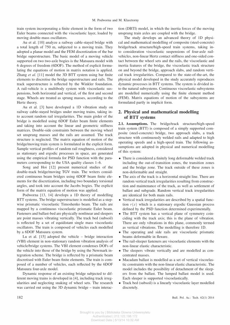
2.2. Concept of physical and numerical modelling. A fi-

nitely long section of the deformable track is depicted in

Fig. 1. The out-of-approach zones have length of 2D. The

first D section from the train entering side enters subsequent

vehicles into the quasi-stationary random vibration state. The

VVRZ zone (Vehicle Vibration Registration Zone) is the area

of registration of the design quantities found in the traffic

safety condition (TSC) and in the passenger comfort condi-

tion (PCC). The BVRZ zone (Bridge Vibration Registration

Zone) is the area of registration of vibrations and stresses in

reference to the bridge superstructure and the platform. The

wheel set/rails interaction forces are recorded during the pas-

sage of the selected axle over the VVRZ zone, including micro

separations of the wheels from the rails and impacts.

Fig. 1. Schematic diagram of BTT system at time t = 0 and t = T

The dynamic process is simulated within the range of

t ∈ [0, T ], where T = (4D + Lo + Lv)/v, with: Lo – bridge

span length plus length of approach slabs plus two sleeper

intervals, Lv – train set length, v – operating velocity (hori-

zontal velocity of moving load).

The remaining symbols in Fig. 1 denote: w(x, t) – vertical

deflection of bridge superstructure, σ(x, t) – longitudinal nor-

mal stresses in bottom fibres of main beams, t – time variable,

x, y – coordinates, ap(x, t) – vertical acceleration of bridge

platform, Rki (t), k = 1, 2, 3, 4, i = 1, 2, . . . , Nv – dynamic

pressures of moving wheel sets, k = 1, 2, 3, 4 – numbering of

wheel sets of ith vehicle, Nv – number of vehicles forming

train, abiα (t), i = 1, 2, . . . , Nv, α = f, r – vertical accel-

erations of suspension pivots in car-bodies (f, r – front/rear

bogie, respectively), T – dynamic process duration time.

Non-stationary vibrations of the bridge caused by the pas-

sage of a high-speed train across the bridge is recorded in

the interval vt ∈ [2D; 4D + Lo + Lv] [m]. The outside sec-

tions D eliminate distortion in the response of vehicles caused

by finitely long sections of the deformable track in the out-

of-approach zones. Transient vibrations of subsequent rail-

vehicles are recorded in intervals of ui = vt − (i − 1) l ∈[D; 3D + Lo] [m], i = 1, 2, . . . , Nv, where l denotes rail-

vehicle length.

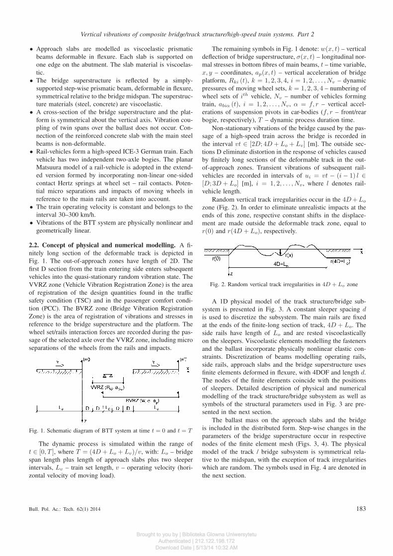
Random vertical track irregularities occur in the 4D +Lo

zone (Fig. 2). In order to eliminate unrealistic impacts at the

ends of this zone, respective constant shifts in the displace-

ment are made outside the deformable track zone, equal to

r(0) and r(4D + Lo), respectively.

Fig. 2. Random vertical track irregularities in 4D + Lo zone

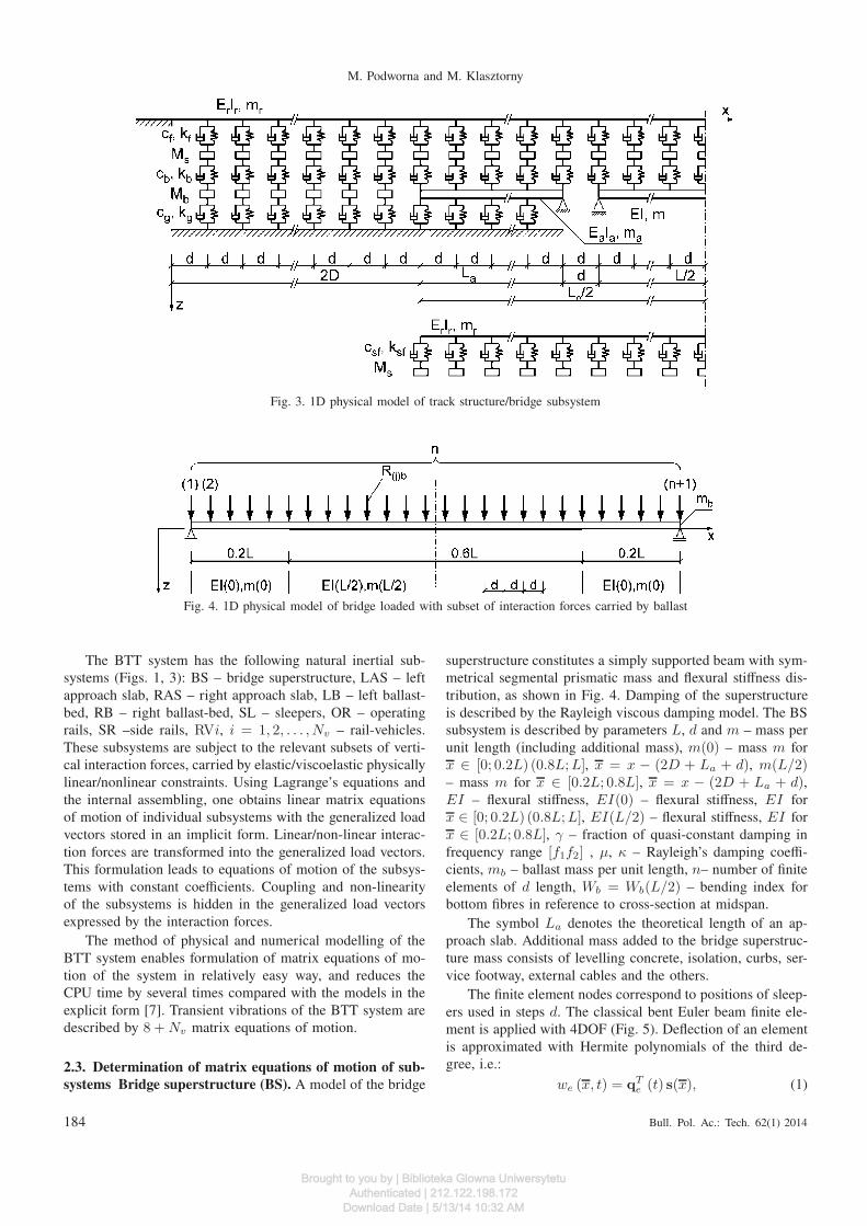
A 1D physical model of the track structure/bridge sub-

system is presented in Fig. 3. A constant sleeper spacing dis used to discretize the subsystem. The main rails are fixed

at the ends of the finite-long section of track, 4D + Lo. The

side rails have length of Lo and are rested viscoelastically

on the sleepers. Viscoelastic elements modelling the fasteners

and the ballast incorporate physically nonlinear elastic con-

straints. Discretization of beams modelling operating rails,

side rails, approach slabs and the bridge superstructure uses

finite elements deformed in flexure, with 4DOF and length d.

The nodes of the finite elements coincide with the positions

of sleepers. Detailed description of physical and numerical

modelling of the track structure/bridge subsystem as well as

symbols of the structural parameters used in Fig. 3 are pre-

sented in the next section.

The ballast mass on the approach slabs and the bridge

is included in the distributed form. Step-wise changes in the

parameters of the bridge superstructure occur in respective

nodes of the finite element mesh (Figs. 3, 4). The physical

model of the track / bridge subsystem is symmetrical rela-

tive to the midspan, with the exception of track irregularities

which are random. The symbols used in Fig. 4 are denoted in

the next section.

Bull. Pol. Ac.: Tech. 62(1) 2014 183




Fig. 3. 1D physical model of track structure/bridge subsystem

Fig. 4. 1D physical model of bridge loaded with subset of interaction forces carried by ballast

The BTT system has the following natural inertial sub-

systems (Figs. 1, 3): BS – bridge superstructure, LAS – left

approach slab, RAS – right approach slab, LB – left ballast-

bed, RB – right ballast-bed, SL – sleepers, OR – operating

rails, SR –side rails, RVi, i = 1, 2, . . . , Nv – rail-vehicles.

These subsystems are subject to the relevant subsets of verti-

cal interaction forces, carried by elastic/viscoelastic physically

linear/nonlinear constraints. Using Lagrange’s equations and

the internal assembling, one obtains linear matrix equations

of motion of individual subsystems with the generalized load

vectors stored in an implicit form. Linear/non-linear interac-

tion forces are transformed into the generalized load vectors.

This formulation leads to equations of motion of the subsys-

tems with constant coefficients. Coupling and non-linearity

of the subsystems is hidden in the generalized load vectors

expressed by the interaction forces.

The method of physical and numerical modelling of the

BTT system enables formulation of matrix equations of mo-

tion of the system in relatively easy way, and reduces the

CPU time by several times compared with the models in the

explicit form [7]. Transient vibrations of the BTT system are

described by 8 + Nv matrix equations of motion.

2.3. Determination of matrix equations of motion of sub-

systems Bridge superstructure (BS). A model of the bridge

superstructure constitutes a simply supported beam with sym-

metrical segmental prismatic mass and flexural stiffness dis-

tribution, as shown in Fig. 4. Damping of the superstructure

is described by the Rayleigh viscous damping model. The BS

subsystem is described by parameters L, d and m – mass per

unit length (including additional mass), m(0) – mass m for

x ∈ [0; 0.2L) (0.8L; L], x = x − (2D + La + d), m(L/2)– mass m for x ∈ [0.2L; 0.8L], x = x − (2D + La + d),EI – flexural stiffness, EI(0) – flexural stiffness, EI for

x ∈ [0; 0.2L) (0.8L; L], EI(L/2) – flexural stiffness, EI for

x ∈ [0.2L; 0.8L], γ – fraction of quasi-constant damping in

frequency range [f1f2] , µ, κ – Rayleigh’s damping coeffi-

cients, mb – ballast mass per unit length, n– number of finite

elements of d length, Wb = Wb(L/2) – bending index for

bottom fibres in reference to cross-section at midspan.

The symbol La denotes the theoretical length of an ap-

proach slab. Additional mass added to the bridge superstruc-

ture mass consists of levelling concrete, isolation, curbs, ser-

vice footway, external cables and the others.

The finite element nodes correspond to positions of sleep-

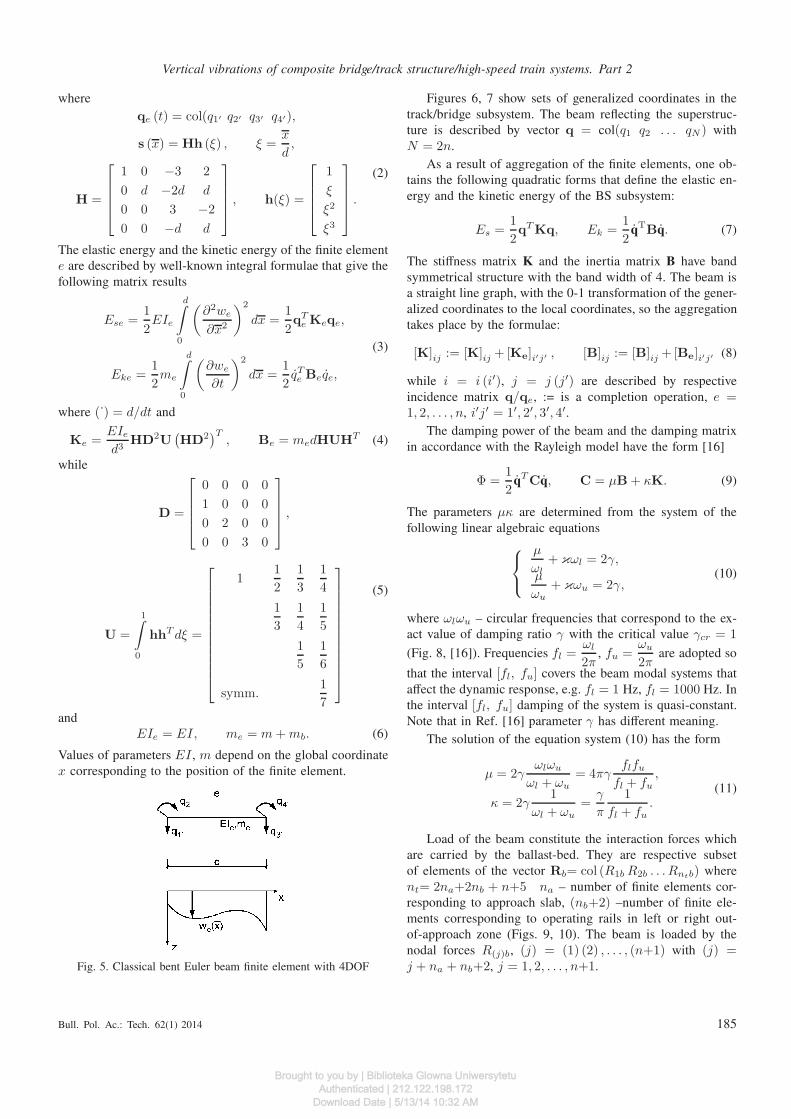
ers used in steps d. The classical bent Euler beam finite ele-

ment is applied with 4DOF (Fig. 5). Deflection of an element

is approximated with Hermite polynomials of the third de-

gree, i.e.:

we (x, t) = qTe (t) s(x), (1)

184 Bull. Pol. Ac.: Tech. 62(1) 2014




where

qe (t) = col(q1′ q2′ q3′ q4′),

s (x) = Hh (ξ) , ξ =x

d,

H =

1 0 −3 2

0 d −2d d

0 0 3 −2

0 0 −d d

, h(ξ) =

1

ξ

ξ2

ξ3

.

(2)

The elastic energy and the kinetic energy of the finite element

e are described by well-known integral formulae that give the

following matrix results

Ese =1

2EIe

d∫

0

(

∂2we

∂x2

)2

dx =1

2qT

e Keqe,

Eke =1

2me

d∫

0

(

∂we

∂t

)2

dx =1

2qTe Beqe,

(3)

where (˙) = d/dt and

Ke =EIe

d3HD2U

(

HD2)T

, Be = medHUHT (4)

while

D =

0 0 0 0

1 0 0 0

0 2 0 0

0 0 3 0

,

U =

1∫

0

hhT dξ =

11

2

1

3

1

4

1

3

1

4

1

5

1

5

1

6

symm.1

7

(5)

and

EIe = EI, me = m + mb. (6)

Values of parameters EI , m depend on the global coordinate

x corresponding to the position of the finite element.

Fig. 5. Classical bent Euler beam finite element with 4DOF

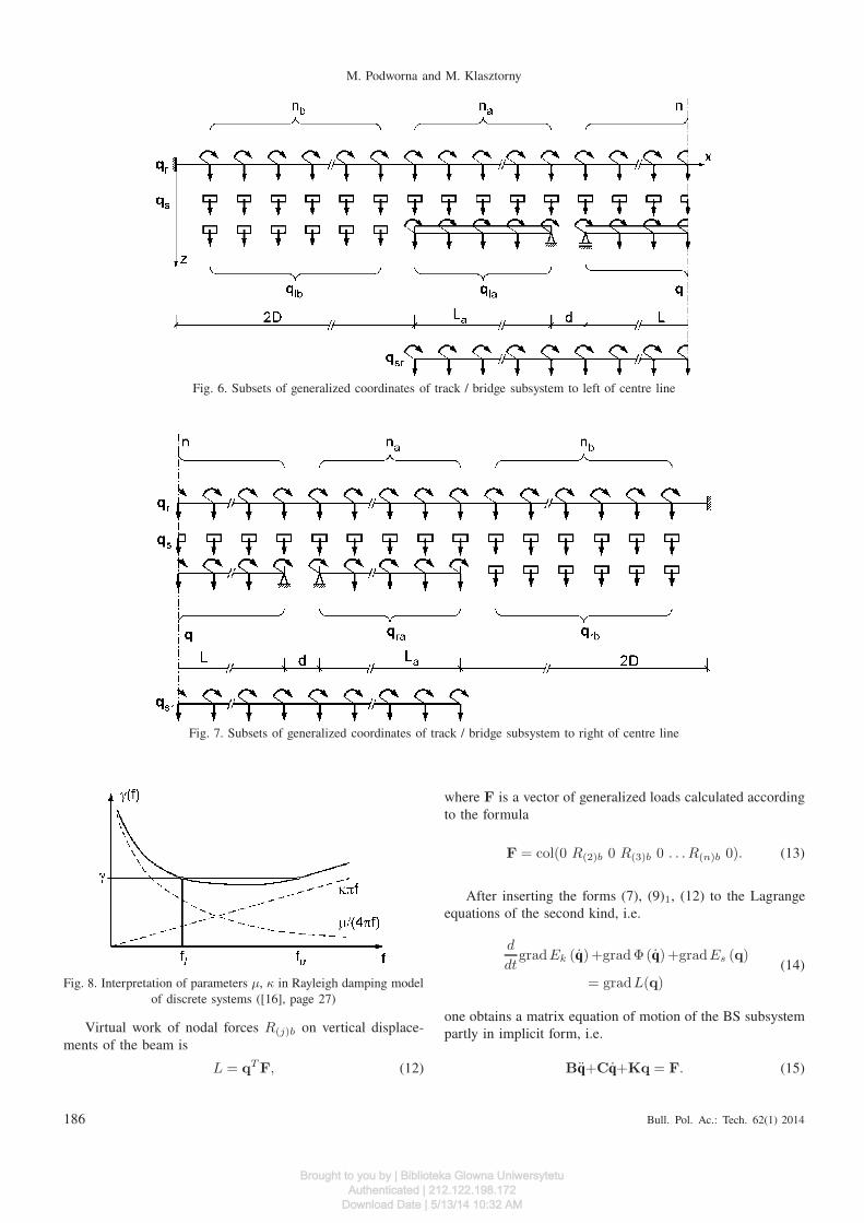
Figures 6, 7 show sets of generalized coordinates in the

track/bridge subsystem. The beam reflecting the superstruc-

ture is described by vector q = col(q1 q2 . . . qN ) with

N = 2n.

As a result of aggregation of the finite elements, one ob-

tains the following quadratic forms that define the elastic en-

ergy and the kinetic energy of the BS subsystem:

Es =1

2qTKq, Ek =

1

2qTBq. (7)

The stiffness matrix K and the inertia matrix B have band

symmetrical structure with the band width of 4. The beam is

a straight line graph, with the 0-1 transformation of the gener-

alized coordinates to the local coordinates, so the aggregation

takes place by the formulae:

[K]ij := [K]ij + [Ke]i′j′ , [B]ij := [B]ij + [Be]i′j′ (8)

while i = i (i′), j = j (j′) are described by respective

incidence matrix q/qe, := is a completion operation, e =1, 2, . . . , n, i′j′ = 1′, 2′, 3′, 4′.

The damping power of the beam and the damping matrix

in accordance with the Rayleigh model have the form [16]

Φ =1

2qTCq, C = µB + κK. (9)

The parameters µκ are determined from the system of the

following linear algebraic equations

µ

ωl+ κωl = 2γ,

µ

ωu+ κωu = 2γ,

(10)

where ωlωu – circular frequencies that correspond to the ex-

act value of damping ratio γ with the critical value γcr = 1

(Fig. 8, [16]). Frequencies fl =ωl

2π, fu =

ωu

2πare adopted so

that the interval [fl, fu] covers the beam modal systems that

affect the dynamic response, e.g. fl = 1 Hz, fl = 1000 Hz. In

the interval [fl, fu] damping of the system is quasi-constant.

Note that in Ref. [16] parameter γ has different meaning.

The solution of the equation system (10) has the form

µ = 2γωlωu

ωl + ωu= 4πγ

flfu

fl + fu,

κ = 2γ1

ωl + ωu=

γ

π

1

fl + fu.

(11)

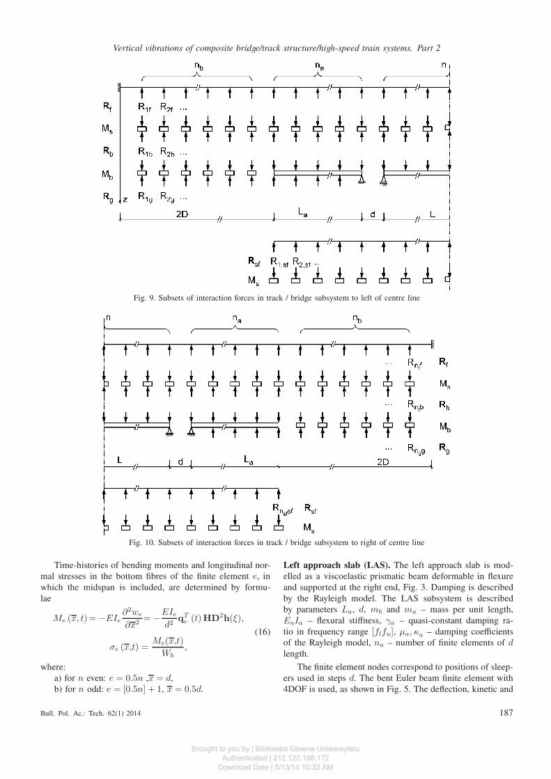
Load of the beam constitute the interaction forces which

are carried by the ballast-bed. They are respective subset

of elements of the vector Rb= col (R1b R2b . . . Rntb) where

nt= 2na+2nb + n+5 na – number of finite elements cor-

responding to approach slab, (nb+2) –number of finite ele-

ments corresponding to operating rails in left or right out-

of-approach zone (Figs. 9, 10). The beam is loaded by the

nodal forces R(j)b, (j) = (1) (2) , . . . , (n+1) with (j) =j + na + nb+2, j = 1, 2, . . . , n+1.

Bull. Pol. Ac.: Tech. 62(1) 2014 185




Fig. 6. Subsets of generalized coordinates of track / bridge subsystem to left of centre line

Fig. 7. Subsets of generalized coordinates of track / bridge subsystem to right of centre line

Fig. 8. Interpretation of parameters µ, κ in Rayleigh damping model

of discrete systems ([16], page 27)

Virtual work of nodal forces R(j)b on vertical displace-

ments of the beam is

L = qT F, (12)

where F is a vector of generalized loads calculated according

to the formula

F = col(0 R(2)b 0 R(3)b 0 . . . R(n)b 0). (13)

After inserting the forms (7), (9)1, (12) to the Lagrange

equations of the second kind, i.e.

d

dtgradEk (q)+grad Φ(q)+gradEs (q)

= gradL(q)(14)

one obtains a matrix equation of motion of the BS subsystem

partly in implicit form, i.e.

Bq+Cq+Kq = F. (15)

186 Bull. Pol. Ac.: Tech. 62(1) 2014




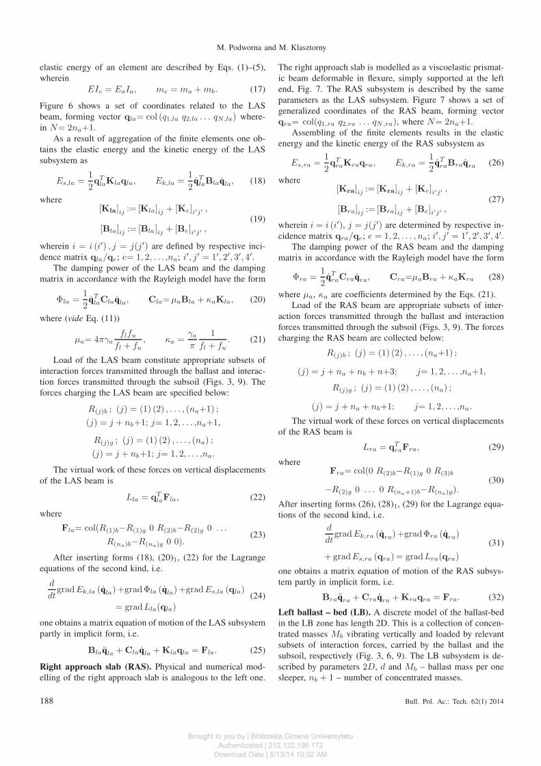
Fig. 9. Subsets of interaction forces in track / bridge subsystem to left of centre line

Fig. 10. Subsets of interaction forces in track / bridge subsystem to right of centre line

Time-histories of bending moments and longitudinal nor-

mal stresses in the bottom fibres of the finite element e, in

which the midspan is included, are determined by formu-

lae

Me (x, t)= −EIe∂2we

∂x2 = −EIe

d2qT

e (t)HD2h(ξ),

σe (x,t) =Me(x,t)

Wb,

(16)

where:

a) for n even: e = 0.5n ,x = d,

b) for n odd: e = [0.5n] + 1, x = 0.5d.

Left approach slab (LAS). The left approach slab is mod-

elled as a viscoelastic prismatic beam deformable in flexure

and supported at the right end, Fig. 3. Damping is described

by the Rayleigh model. The LAS subsystem is described

by parameters La, d, mb and ma – mass per unit length,

EaIa – flexural stiffness, γa – quasi-constant damping ra-

tio in frequency range [flfu], µa, κa – damping coefficients

of the Rayleigh model, na – number of finite elements of dlength.


ers used in steps d. The bent Euler beam finite element with

4DOF is used, as shown in Fig. 5. The deflection, kinetic and

Bull. Pol. Ac.: Tech. 62(1) 2014 187




elastic energy of an element are described by Eqs. (1)–(5),

wherein

EIe = EaIa, me = ma + mb. (17)

Figure 6 shows a set of coordinates related to the LAS

beam, forming vector qla= col (q1,la q2,la . . . qN,la) where-

in N= 2na+1.

As a result of aggregation of the finite elements one ob-

tains the elastic energy and the kinetic energy of the LAS

subsystem as

Es,la =1

2qT

laKlaqla, Ek,la =1

2qT

laBlaqla, (18)

where[Kla]ij := [Kla]ij + [Ke]i′j′ ,

[Bla]ij := [Bla]ij + [Be]i′j′ ,(19)

wherein i = i (i′) , j = j(j′) are defined by respective inci-

dence matrix qla/qe; e= 1, 2, . . . ,na; i′, j′ = 1′, 2′, 3′, 4′.The damping power of the LAS beam and the damping

matrix in accordance with the Rayleigh model have the form

Φla =1

2q

TlaClaqla, Cla=µaBla + κaKla, (20)

where (vide Eq. (11))

µa= 4πγaflfu

fl + fu, κa =

γa

π

1

fl + fu. (21)

Load of the LAS beam constitute appropriate subsets of

interaction forces transmitted through the ballast and interac-

tion forces transmitted through the subsoil (Figs. 3, 9). The

forces charging the LAS beam are specified below:

R(j)b ; (j) = (1) (2) , . . . , (na+1) ;

(j) = j + nb+1; j= 1, 2, . . . ,na+1,

R(j)g ; (j) = (1) (2) , . . . , (na) ;

(j) = j + nb+1; j= 1, 2, . . . ,na.

The virtual work of these forces on vertical displacements

of the LAS beam is

Lla = qTlaFla, (22)

where

Fla= col(R(1)b−R(1)g 0 R(2)b−R(2)g 0 . . .

R(na)b−R(na)g 0 0).(23)

After inserting forms (18), (20)1, (22) for the Lagrange


d

dtgradEk,la (qla)+gradΦla (qla)+gradEs,la (qla)

= gradLla(qla)(24)

one obtains a matrix equation of motion of the LAS subsystem


Blaqla + Claqla + Klaqla = Fla. (25)

Right approach slab (RAS). Physical and numerical mod-

elling of the right approach slab is analogous to the left one.

The right approach slab is modelled as a viscoelastic prismat-

ic beam deformable in flexure, simply supported at the left

end, Fig. 7. The RAS subsystem is described by the same

parameters as the LAS subsystem. Figure 7 shows a set of

generalized coordinates of the RAS beam, forming vector

qra= col(q1,ra q2,ra . . . qN,ra), where N= 2na+1.

Assembling of the finite elements results in the elastic

energy and the kinetic energy of the RAS subsystem as

Es,ra =1

2qT

raKraqra, Ek,ra =1

2q

TraBraqra (26)

where[Kra]ij := [Kra]ij + [Ke]i′j′ ,

[Bra]ij := [Bra]ij + [Be]i′j′ ,(27)

wherein i = i (i′), j = j(j′) are determined by respective in-

cidence matrix qra/qe; e = 1, 2, . . . , na; i′, j′ = 1′, 2′, 3′, 4′.The damping power of the RAS beam and the damping

matrix in accordance with the Rayleigh model have the form

Φra =1

2qT

raCraqra, Cra=µaBra + κaKra (28)

where µa, κa are coefficients determined by the Eqs. (21).

Load of the RAS beam are appropriate subsets of inter-

action forces transmitted through the ballast and interaction

forces transmitted through the subsoil (Figs. 3, 9). The forces

charging the RAS beam are collected below:

R(j)b ; (j) = (1) (2) , . . . , (na+1) ;

(j) = j + na + nb + n+3; j= 1, 2, . . . ,na+1,

R(j)g ; (j) = (1) (2) , . . . , (na) ;

(j) = j + na + nb+1; j= 1, 2, . . . ,na.


of the RAS beam is

Lra = qTraFra, (29)

whereFra= col(0 R(2)b−R(1)g 0 R(3)b

−R(2)g 0 . . . 0 R(na+1)b−R(na)g).(30)

After inserting forms (26), (28)1, (29) for the Lagrange equa-

tions of the second kind, i.e.

d

dtgradEk,ra (qra)+gradΦra (qra)

+ gradEs,ra (qra)= gradLra(qra)

(31)

one obtains a matrix equation of motion of the RAS subsys-

tem partly in implicit form, i.e.

Braqra + Craqra + Kraqra = Fra. (32)

Left ballast – bed (LB). A discrete model of the ballast-bed

in the LB zone has length 2D. This is a collection of concen-

trated masses Mb vibrating vertically and loaded by relevant

subsets of interaction forces, carried by the ballast and the

subsoil, respectively (Fig. 3, 6, 9). The LB subsystem is de-

scribed by parameters 2D, d and Mb – ballast mass per one

sleeper, nb + 1 – number of concentrated masses.

188 Bull. Pol. Ac.: Tech. 62(1) 2014




Figure 6 shows a set of generalized coordinates of the

LB subsystem, creating vector qlb= col(q1,lb q2,lb . . . qN,lb),where N = nb + 1. The kinetic energy and the mass matrix

are

Ek.lb =1

2qT

lbBlbqlb,

Blb= Mb= diag (Mb Mb . . . Mb).

(33)

The LB subsystem is charged by the Rjb, Rjg , j =1, 2, . . . , N forces. The virtual work of these forces on respec-

tive vertical displacements and the generalized load vector are

defined as

Llb = qTlbFlb,

Flb= col(R1b−R1g R2b−R2g . . . RNb−RNg).(34)

After inserting forms (33)1, (34)1 for the Lagrange equations

of the first kind, i.e.

d

dtgradEk,lb (qlb)= gradLlb(qlb) (35)

one obtains a matrix equation of motion of the LB subsystem


Mb qlb = Flb. (36)

Right ballast – bed (RB). Physical and mathematical mod-

elling of ballast-bed in the RB zone is analogous to modelling

of the LB ballast-bed. Ballast-bed RB in the right zone is mod-

elled as a set of concentrated masses Mb vibrating vertically

and loaded by relevant subsets of interaction forces, carried

by the ballast and the subsoil (Figs. 7, 10). The RB subsys-

tem is described by parameters analogous to those for the LB

subsystem.

Figure 7 shows a set of generalized coordinates corre-

sponding to the RB subsystem, creating vector

qrb= col(q1,rb q2,rb . . . qN,rb),

where N = nb + 1. The kinetic energy and the mass matrix

equal

Ek.rb =1

2qT

rbBrbqrb,

Brb= Mb= diag (Mb M b . . . M b).

(37)

The RB subsystem is loaded by the following forces

R(j)b ; (j) = (1) (2) , . . . , (N) ;

(j) = j + 2na + nb + n+4; j= 1, 2, . . . ,N,

R(j)g ; (j) = (1) (2) , . . . , (N) ;

(j) = j + 2na + nb+1; j= 1, 2, . . . ,N.


of masses Mb and the generalized load vector are defined by

the formulae

Lrb = qTrbFrb,

Frb= col(R(1)b−R(1)g R(2)b−R(2)g . . . R(N)b−R(N)g).(38)

After inserting forms (37)1, (38)1 for the Lagrange equations

of the first kind, i.e.

d

dtgradEk,rb (qrb)= gradLrb(qrb) (39)

one obtains a matrix equation of motion of the RB subsystem


Mb qrb = Frb. (40)

Sleepers (SL). Sleepers are modelled as concentrated mass-

es vibrating vertically and loaded with a set of interactions

forces carried by the rail fasteners and the ballast (Figs. 3, 6,

7, 9, 10). Vibrations of the SL subsystem are described by a

matrix equation of motion, partly in implicit form, as a direct

result of the d’Alembert principle, i.e.

Ms qs = Fs, (41)

whereMs= diag (Ms M s . . . Ms),

qs= col (q1s q2s . . . qnts),

Fs = Rf − Rb ,

Rf= col (R1f R2f . . . Rntf ) ,

Rb= col (R1b R2b . . . Rntb),

(42)

wherein

nt = 2na+2nb + n+5,

Rf – interaction force vector transmitted via fasteners, Rb

– interaction force vector carried by ballast qs – generalized

displacement vector describing SL subsystem.

Operating rails (OR). Operating rails are reflected by an

Euler prismatic beam which is fixed to the ends (Fig. 3). The

beam is supported viscoelastically via a set of discrete con-

straints modelling rail fasteners at d intervals. The beam is

loaded by moving rail vehicles. Natural damping of vibra-

tions of operating rails is described by the Rayleigh model.

The OR subsystem is specified by parameter d and (Figs.

1, 3, 6, 7) Lt = 4D + Lo – length of rails, mr – mass

of pair of rails per unit length, ErIr – flexural stiffness of

pair of rails, γr – quasi-constant damping ratio in frequency

range [flfu], µr, κr – damping coefficients in Rayleigh mod-

el, Nt = 2na+2nb + n+6 – number of finite elements of

length d.


ers used in steps d. The bent Euler beam finite element with

4DOF is used (Fig. 5). Deflection of an e-element is described

by Eqs. (1), (2). The elastic energy and the kinetic energy of

an e-element are described by Eqs. (3)–(5), in which should

be substituted

EIe = ErIr, me = mr. (43)

Figures 6, 7, show a set of generalized coordinates of the

OR beam, forming vector qr= col (q1r q2r . . . qNr), where-

in N = 2 (Nt − 1).Assembling of finite elements forming the OR beam leads

to the elastic energy and the kinetic energy of the subsystem

described by the formulas

Bull. Pol. Ac.: Tech. 62(1) 2014 189




Esr =1

2qT

r Krqr , Ekr =1

2q

Tr Brqr . (44)

The stiffness matrix Kr and the mass matrix Br have band

symmetrical structure with band width of 4. The assembling

follows the formulas:

[Kr]ij := [Kr]ij + [Ke]i′j′ ,

[Br]ij := [Br]ij + [Be]i′j′(45)

while i = i (i′), j = j (j′) are defined by respective incidence

matrix qr/qe; e= 1, 2, . . . ,Nt; i′j′ = 1′, 2′, 3′, 4′.The damping power of the OR beam and the damping

matrix in accordance with the Rayleigh model take the form

Φr =1

2q

Tr Crqr, Cr=µrBr + κrKr (46)

where, vide Eq. (11)

µr= 4πγrflfu

fl + fu, κr =

γr

π

1

fl + fu. (47)

Load of the OR subsystem constitute inter-

action forces carried by the rail fasteners, i.e.

Rf= col (R1f R2f . . . Rntf ) and moving pressure forces

of the wheel sets, i.e. Rwi= col (R1i R2i R3i R4i), i =1, 2, . . . , Nv. The virtual work of forces Rki, k= 1, 2, 3, 4 is

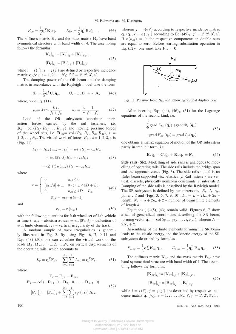
(Fig. 11)

Lki = Rki (wki + rki) = wkiRki + rkiRki

= we (xki,t)Rki + rkiRki

= qTe (t) s (xki)Rki + rkiRki,

(48)

where

e =

0 uki≤ 0,

[uki/d] + 1, 0 < uki<4D + Lo,

0, uki≥ 4D + Lo,

xki = uki−d (e−1)

(49)

and

rki = r (uki) (50)

with the following quantities for k-th wheel set of i-th vehicle

at time t: uki – abscissa x; wki = we (xki,t) – deflection of

e-th finite element; rki – vertical irregularity of the track.

A random sample of track irregularities is general-

ly illustrated in Fig. 2. By using Figs. 6, 7, 9–11 and

Eqs. (48)–(50), one can calculate the virtual work of the

loads Rf ,Rwi , i= 1, 2, . . . ,Nv on vertical displacements of

the operating rails, which accounts to

Lr = qTr Ffr +

Nv∑

i=1

4∑

k=1

Lki = qTr Fr, (51)

where

Fr = Ffr + Fvr,

Ffr= col (−R1f 0 −R2f 0 . . . −Rntf 0),

[Fvr]j := [Fvr]j +

Nv∑

i=1

4∑

k=1

sj′ (xki) Rki,

(52)

wherein j = j(ej′) according to respective incidence matrix

qr/qe, e = e (uki) according to Eq. (49)1, j′ = 1′, 2′, 3′, 4′.If e (uki) = 0, the respective components in double sum

are equal to zero. Before starting substitution operation in

Eq. (52)3, one must take Fvr = 0.

Fig. 11. Pressure force Rki and following vertical displacement

After inserting Eqs. (44), (46)1, (51) for the Lagrange


d

dtgradEkr (qr)+gradΦr (qr)

+ gradEsr (qr)= gradLr(qr)

(53)

one obtains a matrix equation of motion of the OR subsystem


Brqr + Crqr + Krqr = Fr. (54)

Side rails (SR). Modelling of side rails is analogous to mod-

elling of operating rails. The side rails include the bridge span

and the approach zones (Fig. 3). The side rails model is an

Euler beam supported viscoelastically. Rail fasteners are ver-

tical, discrete, physically nonlinear constraints, at intervals d.

Damping of the side rails is described by the Rayleigh model.

The SR subsystem is defined by parameters mr, Er, Ir, γr,

µr, κr, d and (Figs. 3, 6, 7, 9, 10): Lo = L + 2La + 2d –

length, Ns = n + 2na + 2 – number of beam finite elements

of length d.

Equations (1)–(5), (43) remain valid. Figures 6, 7 show

a set of generalized coordinates describing the SR beam,

forming vector qsr= col (q1,sr q2,sr . . . qN,sr), wherein N =2Ns + 2.

Assembling of the finite elements forming the SR beam

leads to the elastic energy and the kinetic energy of the SR

subsystem described by formulas

Es,sr =1

2qT

srKsrqsr, Ek,sr =1

2qT

srBsrqsr . (55)

The stiffness matrix Ksr and the mass matrix Bsr have

band symmetrical structure with band width of 4. The assem-

bling follows the formulas:

[Ksr]ij := [Ksr]ij + [Ke]i′j′ ,

[Bsr]ij := [Bsr]ij + [Be]i′j′(56)

while i = i (i′), j = j (j′) are described by respective inci-

dence matrix qsr/qe; e = 1, 2, . . . , Ns; i′, j′ = 1′, 2′, 3′, 4′.

190 Bull. Pol. Ac.: Tech. 62(1) 2014




The damping power of the SR beam and the damping

matrix in accordance with the Rayleigh model are in the form

Φsr =1

2qT

srCsrqsr, Csr=µrBsr + κrKsr (57)

with coefficients µr, κr determined by Eqs. (47).

Interaction forces carried by the rail fasteners constitute

load of the SR beam, i.e.

Rsf= col (R1,sf R2,sf . . . Rnsf ,sf ),

where nsf = Ns + 1 (Figs. 9, 10). The virtual work of these

forces on vertical displacements of the side rails, and the gen-

eralized load vector are defined as

Lsr = qTsrFsr,

Fsr= col (−R1,sf 0 −R2,sf 0 . . . −Rnsf ,sf 0).(58)

After inserting forms (55), (57)1, (58)1 for the Lagrange


d

dtgradEk,sr (qsr)+gradΦsr (qsr)

+ gradEs,sr (qsr)= gradLsr(qsr)

(59)

one obtains a matrix equation of motion of the SR subsystem

partly in implicit form, i.e.:

Bsrqsr + Csrqsr + Ksrqsr = Fsr. (60)

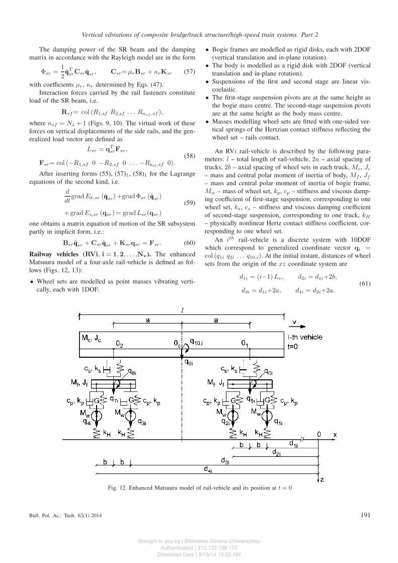
Railway vehicles (RVi, i = 1,2, . . . ,Nv). The enhanced

Matsuura model of a four-axle rail-vehicle is defined as fol-

lows (Figs. 12, 13):

• Wheel sets are modelled as point masses vibrating verti-

cally, each with 1DOF.

• Bogie frames are modelled as rigid disks, each with 2DOF

(vertical translation and in-plane rotation).

• The body is modelled as a rigid disk with 2DOF (vertical

translation and in-plane rotation).

• Suspensions of the first and second stage are linear vis-

coelastic.

• The first-stage suspension pivots are at the same height as

the bogie mass centre. The second-stage suspension pivots

are at the same height as the body mass centre.

• Masses modelling wheel sets are fitted with one-sided ver-

tical springs of the Hertzian contact stiffness reflecting the

wheel set – rails contact.

An RVi rail-vehicle is described by the following para-

meters: l – total length of rail-vehicle, 2a – axial spacing of

trucks, 2b – axial spacing of wheel sets in each truck, Mc, Jc

– mass and central polar moment of inertia of body, Mf , Jf

– mass and central polar moment of inertia of bogie frame,

Mw – mass of wheel set, kp, cp – stiffness and viscous damp-

ing coefficient of first-stage suspension, corresponding to one

wheel set, ks, cs – stiffness and viscous damping coefficient

of second-stage suspension, corresponding to one truck, kH

– physically nonlinear Hertz contact stiffness coefficient, cor-

responding to one wheel set.

An ith rail-vehicle is a discrete system with 10DOF

which correspond to generalized coordinate vector qi =col (q1i q2i . . . q10,i). At the initial instant, distances of wheel

sets from the origin of the xz coordinate system are

d1i = (i−1)Lv, d2i = d1i+2b,

d3i = d1i+2a, d4i = d2i+2a.(61)

Fig. 12. Enhanced Matsuura model of rail-vehicle and its position at t = 0

Bull. Pol. Ac.: Tech. 62(1) 2014 191




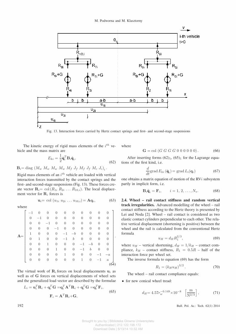
Fig. 13. Interaction forces carried by Hertz contact springs and first- and second-stage suspensions

The kinetic energy of rigid mass elements of the ith ve-

hicle and the mass matrix are

Eki =1

2q

Ti Biqi,

Bi= diag (Mw Mw Mw Mw Mf Jf Mf Jf Mc Jc)i .

(62)

Rigid mass elements of an ith vehicle are loaded with vertical

interaction forces transmitted by the contact springs and the

first- and second-stage suspensions (Fig. 13). These forces cre-

ate vector Ri= col (R1i R2i . . . R10,i). The local displace-

ment vector for Ri forces is

ui= col (u1i u2i . . . u10,i)= Aqi, (63)

where

A=

−1 0 0 0 0 0 0 0 0 0

0 −1 0 0 0 0 0 0 0 0

0 0 −1 0 0 0 0 0 0 0

0 0 0 −1 0 0 0 0 0 0

1 0 0 0 −1 −b 0 0 0 0

0 1 0 0 −1 b 0 0 0 0

0 0 1 0 0 0 −1 −b 0 0

0 0 0 1 0 0 −1 b 0 0

0 0 0 0 1 0 0 0 −1 −a

0 0 0 0 0 0 1 0 −1 a

.

(64)

The virtual work of Ri forces on local displacements ui as

well as of G forces on vertical displacements of wheel sets

and the generalized load vector are described by the formulae

Li = uTi Ri + qT

i G =qTi AT Ri + qT

i G =qTi Fi,

Fi = ATRi+G,(65)

where

G = col (G G G G 0 0 0 0 0 0) . (66)

After inserting forms (62)1, (65)1 for the Lagrange equa-

tions of the first kind, i.e.

d

dtgradEki (qi)= gradLi(qi) (67)

one obtains a matrix equation of motion of the RVi subsystem


Biqi = Fi, i = 1, 2, . . . , Nv. (68)

2.4. Wheel – rail contact stiffness and random vertical

track irregularities. Advanced modelling of the wheel – rail

contact stiffness according to the Hertz theory is presented by

Lei and Noda [2]. Wheel – rail contact is considered as two

elastic contact cylinders perpendicular to each other. The rela-

tive vertical displacement (shortening is positive) between the

wheel and the rail is calculated from the conventional Hertz

formula

uH = dHR2/31 , (69)

where uH – vertical shortening, dH = 1/kH – contact com-

pliance, kH – contact stiffness, R1 = 0.5R – half of the

interaction force per wheel set.

The inverse formula to equation (69) has the form

R1 = (kHuH)3/2

. (70)

The wheel – rail contact compliance equals:

• for new conical wheel tread:

dH= 4.57r−0.149w ×10−8

[ m

N2/3

]

, (71)

192 Bull. Pol. Ac.: Tech. 62(1) 2014




• for the wheel of worn tread:

dH= 3.86r−0.115w ×10−8

[ m

N2/3

]

, (72)

where rw [m] – nominal wheel radius. For an ICE-3 train

wheel radius rw = 0.46 m and:

• for new conical wheel tread: kH = 0.195× 108[

N2/3

m

]

• for the wheel of worn tread: kH = 0.237× 108[

N2/3

m

]

.

In [16], the average value is used, i.e. kH = 0.216 ×

108[

N2/3

m

]

.

In reference to modelling of random track irregularity

samples, only the vertical profile (elevation irregularity), i.e.

the mean vertical elevation of two rails, is taken into con-

sideration. Short wavelength corrugation irregularities in rail

and design geometry irregularities in track formation are ne-

glected. A stationary and ergodic Gaussian process in space

is characterised by one-sided PSD function Srr(Ω), with

Ω = 2π/Lr [rad/m] as a spatial frequency, and Lr as wave-

length. The most common definition of Srr(Ω) is presented

by Fryba [18] and was elaborated by Federal Railroad Ad-

ministration (FRA USA), in the form

Srr (Ω) = kAΩ2

c(

Ω2+Ω2c

)

Ω2

[

mm2m

rad

]

, (73)

where k = 0.25, Ωc = 0.8245 [rad/m]. Coefficient A[mm2rad/m] is specified for line grades 1 – 6. Only better

railway lines of grades 4 (A = 53.76), 5 (A = 20.95) and 6

(A = 3.39) are considered in [16].

Random samples of track irregularity vertical profile are

generated with the Monte-Carlo method which results in the

following formula [18]

r (x) = 2

Nr∑

i=1

√

Srr (Ωi)∆Ωcos (Ωix + φi) [mm], (74)

where Ωi = Ωmin + (i − 0.5)∆Ω – discrete frequen-

cy, φi – random phase angle uniformly distributed over

[0, 2π] [rad] interval and independent for i = 1, 2, . . . , Nr,

∆Ω =1

Nr(Ωmax − Ωmin) – frequency increment, Nr – to-

tal number of frequency increments in [Ωmin, Ωmax] interval,

Ωmin =2π

Lr,maxΩmax =

2π

Lr,min– lower and upper limits of

spatial frequency, Lr,min, Lr,max – lower and upper limits of

wavelength.

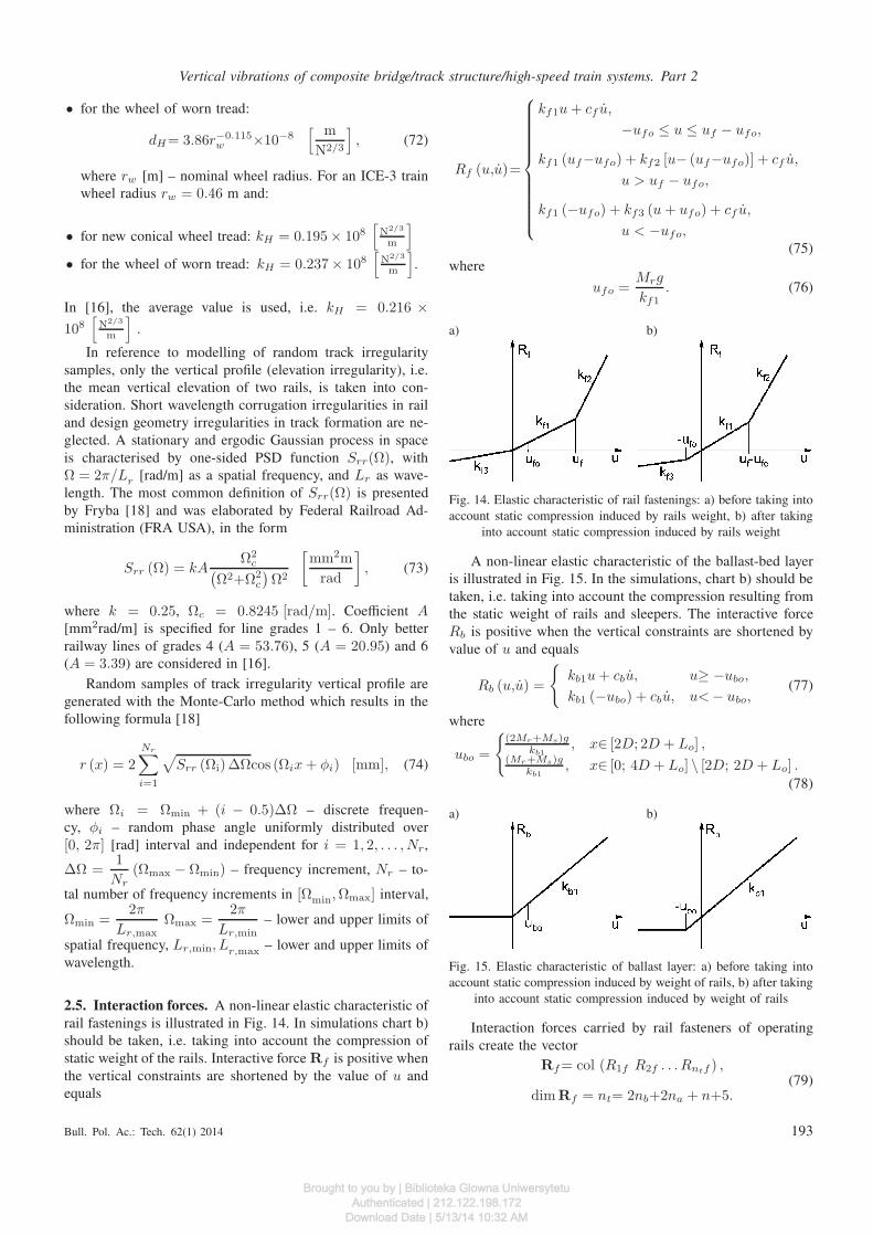
2.5. Interaction forces. A non-linear elastic characteristic of

rail fastenings is illustrated in Fig. 14. In simulations chart b)

should be taken, i.e. taking into account the compression of

static weight of the rails. Interactive force Rf is positive when

the vertical constraints are shortened by the value of u and

equals

Rf (u,u)=

kf1u + cf u,

−ufo ≤ u ≤ uf − ufo,

kf1 (uf−ufo) + kf2 [u− (uf−ufo)] + cf u,

u > uf − ufo,

kf1 (−ufo) + kf3 (u + ufo) + cf u,

u < −ufo,(75)

where

ufo =Mrg

kf1. (76)

a) b)

Fig. 14. Elastic characteristic of rail fastenings: a) before taking into

account static compression induced by rails weight, b) after taking

into account static compression induced by rails weight

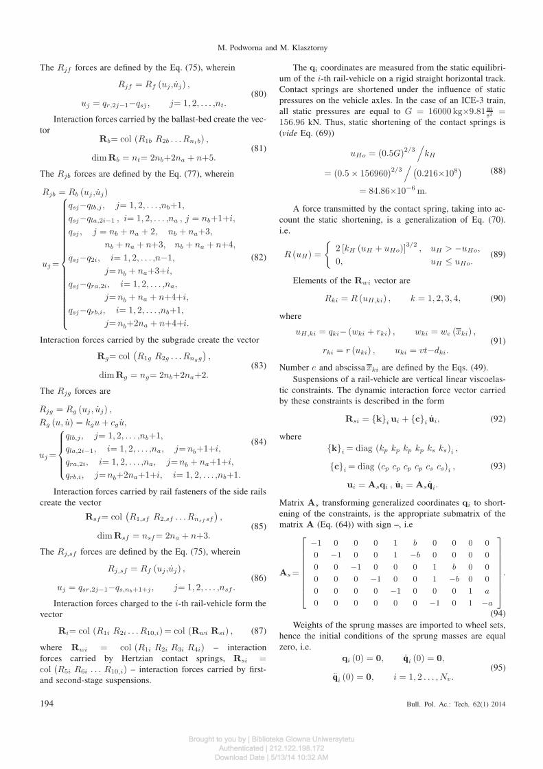
A non-linear elastic characteristic of the ballast-bed layer

is illustrated in Fig. 15. In the simulations, chart b) should be

taken, i.e. taking into account the compression resulting from

the static weight of rails and sleepers. The interactive force

Rb is positive when the vertical constraints are shortened by

value of u and equals

Rb (u,u) =

kb1u + cbu, u≥ −ubo,

kb1 (−ubo) + cbu, u< − ubo,(77)

where

ubo =

(2Mr+Ms)gkb1

, x∈ [2D; 2D + Lo] ,(Mr+Ms)g

kb1, x∈ [0; 4D + Lo] \ [2D; 2D + Lo] .

(78)

a) b)

Fig. 15. Elastic characteristic of ballast layer: a) before taking into

account static compression induced by weight of rails, b) after taking

into account static compression induced by weight of rails

Interaction forces carried by rail fasteners of operating

rails create the vector

Rf= col (R1f R2f . . . Rntf ) ,

dimRf = nt= 2nb+2na + n+5.(79)

Bull. Pol. Ac.: Tech. 62(1) 2014 193




The Rjf forces are defined by the Eq. (75), wherein

Rjf = Rf (uj ,uj) ,

uj = qr,2j−1−qsj , j= 1, 2, . . . ,nt.(80)

Interaction forces carried by the ballast-bed create the vec-

torRb= col (R1b R2b . . . Rntb) ,

dimRb = nt= 2nb+2na + n+5.(81)

The Rjb forces are defined by the Eq. (77), wherein

Rjb = Rb (uj,uj)

uj =

qsj−qlb,j , j= 1, 2, . . . ,nb+1,

qsj−qla,2i−1 , i= 1, 2, . . . ,na , j = nb+1+i,

qsj , j = nb + na + 2, nb + na+3,

nb + na + n+3, nb + na + n+4,

qsj−q2i, i= 1, 2, . . . ,n−1,

j=nb + na+3+i,

qsj−qra,2i, i= 1, 2, . . . ,na,

j=nb + na + n+4+i,

qsj−qrb,i, i= 1, 2, . . . ,nb+1,

j=nb+2na + n+4+i.

(82)

Interaction forces carried by the subgrade create the vector

Rg= col(

R1g R2g . . . Rngg

)

,

dimRg = ng= 2nb+2na+2.(83)

The Rjg forces are

Rjg = Rg (uj , uj) ,

Rg (u, u) = kgu + cgu,

uj =

qlb,j , j= 1, 2, . . . ,nb+1,

qla,2i−1, i= 1, 2, . . . ,na, j= nb+1+i,

qra,2i, i= 1, 2, . . . ,na, j=nb + na+1+i,

qrb,i, j=nb+2na+1+i, i= 1, 2, . . . ,nb+1.

(84)

Interaction forces carried by rail fasteners of the side rails

create the vector

Rsf= col(

R1,sf R2,sf . . . Rnsf sf

)

,

dimRsf = nsf= 2na + n+3.(85)

The Rj,sf forces are defined by the Eq. (75), wherein

Rj,sf = Rf (uj,uj) ,

uj = qsr,2j−1−qs,nb+1+j , j= 1, 2, . . . ,nsf .(86)

Interaction forces charged to the i-th rail-vehicle form the

vector

Ri= col (R1i R2i . . . R10,i) = col (Rwi Rsi) , (87)

where Rwi = col (R1i R2i R3i R4i) – interaction

forces carried by Hertzian contact springs, Rsi =col (R5i R6i . . . R10,i) – interaction forces carried by first-

and second-stage suspensions.

The qi coordinates are measured from the static equilibri-

um of the i-th rail-vehicle on a rigid straight horizontal track.

Contact springs are shortened under the influence of static

pressures on the vehicle axles. In the case of an ICE-3 train,

all static pressures are equal to G = 16000 kg×9.81ms2 =

156.96 kN. Thus, static shortening of the contact springs is

(vide Eq. (69))

uHo = (0.5G)2/3/

kH

= (0.5 × 156960)2/3

/

(

0.216×108)

= 84.86×10−6 m.

(88)

A force transmitted by the contact spring, taking into ac-

count the static shortening, is a generalization of Eq. (70).

i.e.

R (uH) =

2 [kH (uH + uHo)]3/2

, uH > −uHo,

0, uH ≤ uHo.(89)

Elements of the Rwi vector are

Rki = R (uH,ki) , k = 1, 2, 3, 4, (90)

where

uH,ki = qki− (wki + rki) , wki = we (xki) ,

rki = r (uki) , uki = vt−dki.(91)

Number e and abscissa xki are defined by the Eqs. (49).

Suspensions of a rail-vehicle are vertical linear viscoelas-

tic constraints. The dynamic interaction force vector carried

by these constraints is described in the form

Rsi = ki ui + ci ui, (92)

where

ki = diag (kp kp kp kp ks ks)i ,

ci = diag (cp cp cp cp cs cs)i ,

ui = Asqi , ui = Asqi.

(93)

Matrix As transforming generalized coordinates qi to short-

ening of the constraints, is the appropriate submatrix of the

matrix A (Eq. (64)) with sign –, i.e

As =

−1 0 0 0 1 b 0 0 0 0

0 −1 0 0 1 −b 0 0 0 0

0 0 −1 0 0 0 1 b 0 0

0 0 0 −1 0 0 1 −b 0 0

0 0 0 0 −1 0 0 0 1 a

0 0 0 0 0 0 −1 0 1 −a

.

(94)

Weights of the sprung masses are imported to wheel sets,

hence the initial conditions of the sprung masses are equal

zero, i.e.

qi (0) = 0, qi (0) = 0,

qi (0) = 0, i = 1, 2 . . . , Nv.(95)

194 Bull. Pol. Ac.: Tech. 62(1) 2014




2.6. Numerical integration of equations of motion. As

proved in previous points, transient vibrations of the BTT

system are governed by 8 + Nv matrix equations of motion,

where Nv is number of rail-vehicles. These equations are part-

ly in implicit form. The coupling is hidden in the generalized

load vectors expressed by the interaction forces Rf , Rsf , Rb,

Rg, Ri, i = 1, 2, . . . , Nv. Matrix equations of motion of the

subsystems belong to the class of linear ordinary differential

equations with constant coefficients, i.e.

Bq(t) + Cq(t) + Kq(t) = F (R (t) ,t) , (96)

where B, C, K – mass, damping and stiffness matrices for an

inertial subsystem, F (R (t) ,t) – generalized load vector, re-

lated to a subsystem, generally dependent on interaction forces

vector R(t) and time variable t.At the initial instant, the train has a constant horizontal

operating velocity v and it is on the left straight rigid track.

The BTT system is in equilibrium and is described so that

each subsystem corresponds to zero initial conditions, i.e.

q (0)= 0, q (0)= 0. (97)

In addition, F (R (0) , 0)= 0, and hence from Eq. (96) at the

initial instant one obtains

q (0)= 0. (98)

To date, numerous one-step and multi-step methods for

numerical integration of equations of motion of discrete sys-

tems have been developed. One-step methods are natural for

these equations due to initial conditions. One-step methods

are divided into two groups, i.e. methods without numerical

(spurious) damping (e.g. a set of Newmark’s methods with

parameter γN = 1/2) and methods with numerical damping

(e.g. a set of Newmark’s methods with parameter γN 6= 1/2)

[19]. Methods without numerical damping are analysed due

to the stability limit, the amplitude error and the period error.

A finite stability limit causes a rapid growth of numerical inte-

gration errors nearby this limit. The amplitude error influences

accuracy, however, it does not accumulate itself during the in-

tegration process. The period error crucially influences accu-

racy since it accumulates itself during the integration process.

The implicit matrix equation of motion (96) will be

integrated numerically at initial conditions (97, 98) using

the Newmark average acceleration method with parameters

βN=1/4, γN = 1/2, developed to the implicit form as pre-

sented in [14]. The amplitude error vanishes, while the period

error decreases as a time step decreases. The influence of the

period error can be freely reduced via assuming a relatively

small integration step determined from preliminary numerical

tests. Note that in the case of explicit equations this method

is unconditionally stable.

Dynamic response of an N -DOF system described by gov-

erning Eq. (96) is determined in equidistant time points in the

[0, T ] interval, i.e.

ti+1 = (i+1)h, i= 0, 1, . . . , Nc−1, (99)

where T is time of the dynamic process duration, h = ∆t is

a time step, Nc = T/h is number of integration steps. The

following discrete values are introduced

qi= q (ti) , qi = q (ti) , qi = q (ti) ,

Ri= R (ti) , Fi= F (Ri,ti) .(100)

The Newmark recurrent formulae for βN = 1/4, γN =1/2 have the form [18]

qi+1 = qi + hqi +1

4h2

(

qi + qi+1

)

,

qi+1 = qi +1

2h

(

qi + qi+1

)

.(101)

Acceleration vector qi+1 is determined from the collocation

condition at the end of the i-th time step what results in an

algebraic system of linear equations, i.e.

Uqi+1 = Vi+1 =⇒ qi+1 = U−1Vi+1 , (102)

where

U = B+1

2hC+

1

4h2K,

Vi+1 = Fi+1−C

(

qi +1

2hqi

)

−K

(

qi + hqi +1

4h2qi

)

.

(103)

Matrix U is reversed only once. Based on Eqs. (97, 98) the

extended initial conditions take the form

q0 = 0, q0 = 0, q0 = 0. (104)

An algorithm for numerical integration of Eq. (96) is im-

plicit due to interaction vector Ri+1 that defines vector Fi+1.

A linear prediction of vector Ri+1 is used, i.e. [14]

Rpi+1= 2R

i−Ri−1 (105)

with R−1 = R0 due to static equilibrium of the system in the

t ≤ 0 interval. The implicit algorithm for numerical integra-

tion of Eq. (96) consists of the following calculation stages:

1. predict Ri+1 using Eq. (105),

2. calculate qi+1 using Eqs. (102), (103) with Ri+1 = Rpi+1,

3. calculate qi+1, qi+1 using Eqs. (101),

4. correct Ri+1 calculating the forces by definitions (one ob-

tains Rci+1),

5. check the iteration end condition

∣

∣Rcj,i+1−Rp

j,i+1

∣

∣≤ε, j= 1, 2, . . . , N, (106)

where ε > 0 – accuracy parameter determined from prelimi-

nary numerical simulations; if relationship (106) is satisfied,

go to next time step; if relationship (106) is not satisfied,

substitute

Rpi+1 := Rc

i+1 (107)

and go to stage 2.

Bull. Pol. Ac.: Tech. 62(1) 2014 195




3. Conclusions

1. The study develops an advanced theory of 1D quasi-exact

physical and mathematical modelling of composite bridge

/ track structure / high-speed train systems (BTT), includ-

ing viscoelastic suspensions of rail-vehicles equipped with

two two-axle bogies, non-linear Hertz contact stiffness and

one-sided contact between the wheel sets and the rails, vis-

coelastic and inertia features of the bridge, the track struc-

ture on and beyond the bridge, approach slabs, and random

vertical track irregularities. Compared to the state-of-the-

art, the physical model developed in this study accurately

reproduces dynamic processes in real systems.

2. A method of formulation of equations of motion partly in

implicit form has appeared to be effective for BTT systems.

Vibrations in the vertical plane of symmetry are described

by more than nine matrix equations of motion with constant

coefficients. The couplings and non-linearities are hidden

in the generalized load vectors. The equations of motion

are of high clearance, easy to mechanical and mathematical

interpretations. They are integrated using the implicit New-

mark average acceleration method with linear extrapolation

of the interaction forces.

3. Simulation of deterministic and random vibrations of the

exemplary BTT system is presented in [5, 17].

Acknowledgements. The study was supported by the Na-

tional Centre for Science, Poland, as a part of the project

No. N N506 0992 40, realized in the period 2011-2013. This

support is gratefully acknowledged.

REFERENCES

[1] A. Wiriyachai, K.H. Chu, and V.K. Gang, “Bridge impact due

to wheel and track irregularities”, ASCE J. Engng. Mech. Div.

108 (4), 648–666, 1982.

[2] X. Lei and N.-A. Noda, “Analyses of dynamic response of ve-

hicle and track coupling system with random irregularity of

track vertical profile”, J. Sound Vib. 258 (1), 147–165, 2002.

[3] F.T.K. Au, J.J. Wang, and Y.K. Cheung, “Impact study of cable

stayed railway bridges with random rail irregularities”, Engi-

neering Structures 24, 529–541 (2002).

[4] M. Majka and M. Hartnett, “Dynamic response of bridges to

moving trains: A study on effects of random track irregularities

and bridge skewness”, Comput. Struct. 87, 1233–1253 (2009).

[5] M. Podworna and M. Klasztorny, “Vertical vibrations of com-

posite bridge / track structure / high-speed train system. Part 1:

Series-of-types of steel-concrete bridges”, Bull. Pol. Ac.: Tech.

62 (1), 165–179 (2014).

[6] M. Klasztorny, Vibrations of Railway Single-track Bridges In-

duced by Trains Moving at High-speeds, WPWr Press, Wro-

claw, 1987, (in Polish).

[7] M. Klasztorny, Dynamics of Beam Bridges under High-speed

Trains, WNT Press, Warsaw, 2005, (in Polish).

[8] L. Fryba, “A rough assessment of railway bridges for high

speed trains”, Engineering Structures 23, 548–556 (2001).

[9] Y.S. Cheng, F.T.K. Au, and Y.K. Cheung, “Vibration of rail-

way bridges under a moving train by using bridge-track-vehicle

element”, Engineering Structures 23 (12), 1597–1606 (2001).

[10] F.T.K. Au, J.J. Wang, and Y.K. Cheung, “Impact study of

cable-stayed bridge under railway traffic using various mod-

els”, J. Sound Vib. 240 (3), 447–465 (2001).

[11] Q.-L. Zhang, A. Vrouwenvelder, and J. Wardenier, “Numeri-

cal simulation of train – bridge interactive dynamics”, Comput.

Struct. 79, 1059–1075 (2001).

[12] M.-K. Song and C.-K. Choi, “Analysis of high-speed vehicle-

bridge interactions by a simplified 3-D model”, Structural En-

gineering and Mechanics 13 (5), 505–532 (2002).

[13] M. Podworna, “Vertical vibrations of steel beam bridges in-

duced by trains moving at high speeds. Part 1 – theory”,

Archives of Civil Engineering 51 (2), 179–209 (2005).

[14] M. Podworna, “Vertical vibrations of steel beam bridges in-

duced by trains moving at high speeds. Part 2 – numeri-

cal analysis”, Archives of Civil Engineering 51 (2), 211–231

(2005).

[15] F. Lu, J.H. Lin, D. Kennedy, and F.W. Williams, “An algorithm

to study non-stationary random vibrations of vehicle – bridge

system”, Comput. Struct. 87, 177–185 (2009).

[16] J. Langer, Dynamics of Structures, Wroclaw Univ. Technol.

Press, Wroclaw, 1980, (in Polish).

[17] M. Podworna and M. Klasztorny, “Vertical vibrations of com-

posite bridge / track structure / high-speed train system. Part

3: Deterministic and random vibrations of exemplary system”,

Bull. Pol. Ac.: Tech. 62 (2), (2014), (to be published).

[18] L. Fryba, Dynamics of Railway Bridges, Academia, Praha,

1996.

[19] N.M. Newmark, “A method of computation for structural dy-

namics”, ASCE J. Eng. Mech. Div. 85 (3), 67–94 (1959).

196 Bull. Pol. Ac.: Tech. 62(1) 2014



vertical vibrations of composite bridge/track...

Documents