vibrating pendulum and stratified fluids
TRANSCRIPT
Vibrating pendulum and stratified fluids
Inga Koszalka
1 Abstract
The problem posed is the stabilization of the inverted state of a simple pendulum inducedby high–frequency vertical oscillations of the pivot point. The stability conditions are de-rived by means of the multiscale perturbation leading to the averaged dynamics as well asby linearization. Then the concept and methods are applied to the study of an incompress-ible, inviscid, stratified fluid under the Boussinesq approximation. The mechanism of thestabilization of the fluid system was found to be analogous to that of pendulum providedthat the density disturbance has the form of a wave or the sum of waves. However, theanalogy in case of a general density disturbance is not obvious.
2 Introduction
A simple pendulum has only one stable state, the straight–down position. However, ifits support vibrates in the vertical or, equivalently, when the gravity is modulated at afrequency much greater than the natural frequency of the pendulum, then it is also possiblefor the inverted (upside–down) position to be a stable state. The problem dates back to1908 when Stephenson showed that it is indeed possible to stabilize an inverted pendulumby subjecting the pivot to small vertical oscillations of suitably high frequency ([17], [18],[19]). However, it was the work of Piotr Kapitza ([10]) that drew broader attention andcommenced a series of studies concerned with this interesting phenomenon, called sometimesfor that reason ”Kapitza pendulum”. Similar behavior of parametrically forced systems inthis parameter regime was found in other problems, like particle trapping and even evolutionof market prices (e.g see [6], [7]).
The purpose of this work is to investigate the stabilization of the inverted pendulum andto apply the concept and the methods developed to fluid dynamics. The pendulum systemis treated by means of the multiscale perturbation which leads to the averaged dynamics,as well as by linearization, which reduces the problem to Mathieu equation. As a simplefluid analog we choose incompressible, stratified fluid under the Boussinesq approximationin periodic domain, subjected to a rapidly varying gravitational field. We focus on themultiscale technique and averaged dynamics to find the stabilization mechanism equivalentto that obtained for the Kapitza pendulum.
205
Grid ( 1 , 1 )
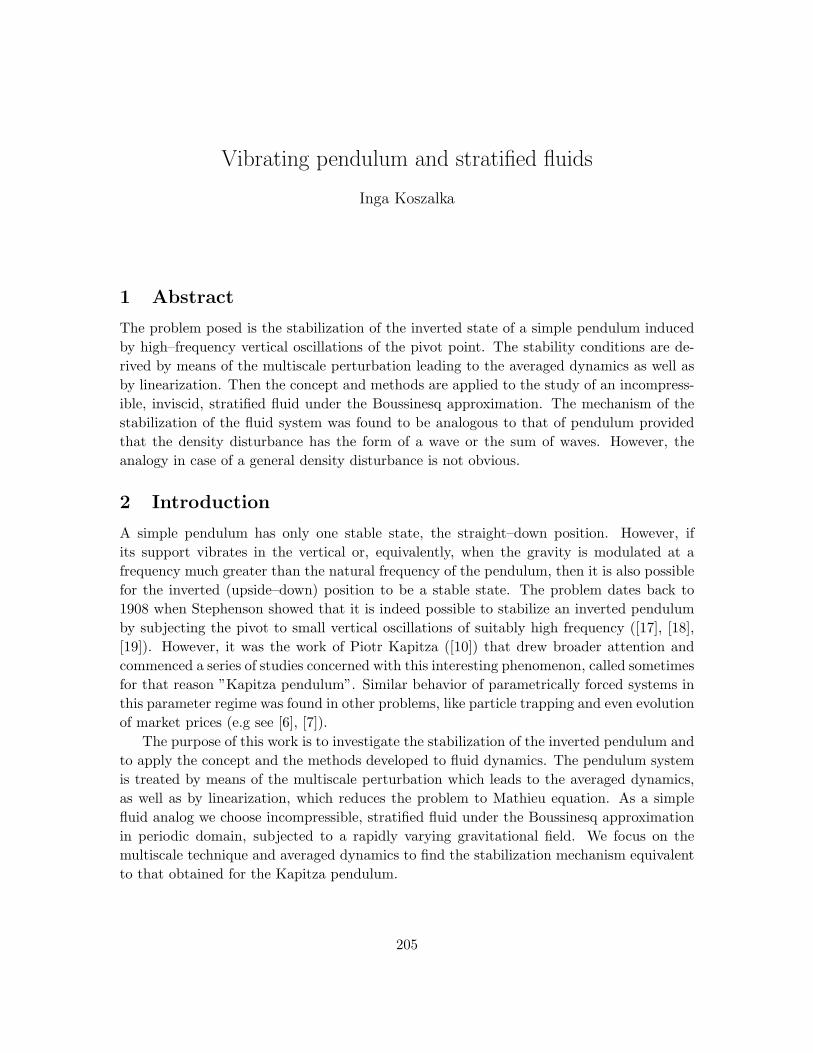
Figure 1: Kapitza pendulum.
3 Vibrating inverted pendulum
3.1 Problem formulation. Equation of motion
We consider a simple, nonlinear pendulum of mass m and length l, moving on a verticalplane in the uniform gravitational field and subjected to a vertical, rapid vibration of thepivot point. By rapid vibration we mean oscillation of high frequency and small amplitudeof the pivot motion, given a form:
ζ(t) = a cos(γt). (1)
The parameters of the external forcing, the amplitude of the vertical motion and the fre-quency, obey
a ∼ O(ε), γ ∼ O(1ε),
where ε is a small number. Following the classical work of [11], we choose the coordinatesystem depicted in figure 1 and the following transformation:
x = l sinφ
y = l cosφ+ a cos(γt), (2)
where φ ∈ R/2πZ is the angle that the pendulum forms with the downward vertical. Fromthe Lagrangian of the system (for the derivation, see Appendix A), we obtain the equationof motion of the vibrationally forced pendulum:
ml2φ+mgol sinφ+malγ2 cos(γt) sinφ = 0, (3)
where go is the gravitational constant. It is worth noting that by a simple rearrengementleading to:
lφ+(go − aγ2 cos(γt)) sinφ = 0,
we can regard the system of the pendulum with the vertically oscillating support as aimmotile pendulum in the field of a modulated, rapidly varying modified gravity of theform:
g = go +1εg−1(
t
ε).
206
Defing the natural frequency ωo of the pendulum by ω2o = go
l , we get a more concise formof the equation of motion:
φ+ (ω2o +
a
lγ2 cos(γt)) sinφ = 0. (4)
It is more convenient to operate with non–dimensional parameters. Without the loss ofgenerality, we let ω2
o = 1 and divide (4) by it. The nondimensional time is set to be t∗ = ωot.We define the ratio of forcing and natural frequencies Ω, and the relative amplitude of theforcing β as, respectively:
Ω =γ
ωo= γ, β =
a
l,
where Ω ∼ O(1ε ) and β ∼ O(ε). Dropping asterics, the equation of motion of the so–called
”normalized pendulum” becomes:
φ+ (1 + βΩ2 cos(Ω t)) sinφ = 0. (5)
This is a nonlinear equation with periodic coefficients, and is nonintegrable. Note that itdescribes a forced motion in a uniform field of gravitational potential Uo:
∂2φ
∂t2= −∂Uo
∂φ− βΩ2 cos(Ω t) sinφ, where Uo = − cosφ (6)
The stability properties of this system have been studied either by means of averaging (e.g.[10], [11]), i.e. effective potential method, or by linearization around fixed points whichleads to Mathieu equation (e. g. [18], [8]). The information obtained by neither of thetwo approaches is complete, however it is in some sense complementary; therefore we foundworthwile to apply both of them. We obtain the averaged dynamics by an alternative tech-nique, the multiscale perturbation, and then zoom into the neighborhood of the equilibraby means of linearization.
3.2 1ε
problem and multiscale perturbation
We note that there are two well separated time scales in our problem, corresponding tothe slow motion of the pendulum and fast oscillation of the pivot point. We can thereforeattempt to find an asymptotic solution valid on long time scales of the pendulum motion.We will define a perturbation parameter and its relation with the forcing parameters by:
ε =1Ω, |ε| 1, β =
a
l= εβ. (7)
The independent time scales in our problem are:
slow time: t, t ∼ O(1)
fast time: τ =t
ε, τ ∼ O(
1ε),
and so the equation of motion (4) can be expressed as:
φ+ (1 +β
εcos τ) sinφ = 0. (8)
207
The first and the second time derivatives become, respectively:
d
dt=
∂
∂t+
1ε
∂
∂τ,
d2
dt2=
∂2
∂t2+
2ε
∂2
∂τ∂t+
1ε2
∂2
∂τ2.
Expanding the variable φ in power series of ε yields:
φ(t, τ) = φo(t, τ) + εφ1(t, τ) + ε2φ2(t, τ) + . . . . (9)
Inserting the perturbation series (9) into (8) and assembling powers of ε yields a set ofequations for the subsequent orders in ε. Manipulation of these equations results in a groupof terms that give unbounded, linear growth of the solution in fast time τ which obviouslydestroys the solution on long time scales. Such terms are called secular terms and a standardprocedure in multiscale perturbation technique is to remove them by making them equal tozero and vanish ([9]). For the justification and more detailed treatment of the problem, seeAppendix B. The condition for the solution to be valid uniformly on t gives the equation ofmotion of the leading order quantity:
∂2φo
∂t2= −(1 +
(βΩ)2
2cosφo) sinφo. (10)
It is worth to note that the same result would be obtained if the average of the O(1)equation over the fast time has been taken, defined as following:
ε T 1, ψ(t) ≡ 1T
∫ τ+T
τψ(t, τ ′)dτ ′, (11)
(see Appendix B). Using the fact that cos2 τ = 12 , we get:
∂2φ
∂t2= −(1 +
(βΩ)2
2cosφ) sinφ. (12)
Therefore, we can consider (10), governing the dynamics of the O(1) quantity, to be equiv-alent to the dynamics of a variable averaged over the fast oscillations (12).
3.3 Averaged dynamics. Effective potential.
We can note the averaged dynamics of the vibrationally forced pendulum governed by (12),can be perceived as a motion in the field of effective potential U :
∂2φ
∂t2= −∂U
∂φ, where U = − cosφ+
β2Ω2
4sin2 φ. (13)
Interestingly, there is no explicit time dependence in the governing equation, as the effectivepotential is dependent only on the mean state of the system and parameters of the forcing(compare with (6)). This observation allows for the following physical explanation of theprocess, given by [10]. Vibrational gravitational field (induced by the oscillatory motion ofthe pivot) leads to the production the vibrational torgue which on average manifests as anordinary force. This force tends to set the rod of the pendulum in the direction of the axis ofthe oscillations. Provided the vibrational force is balanced by the gravity, the inverted stateexhibits the dynamical equilibrum and becomes stable. We can now express the stabilitycondition for the upper equilibrum in terms of the parameters of the forced system. Let’stake a closer look into the stability of the system.
208
0 1.57 3.14 4.71 6.28−4
−3
−2
−1
0
φ
U(φ
)
unforced pendulum
0 1.57 3.14 4.71 6.28−0.4
−0.2
0
0.2
φ
vertically forced pendulum
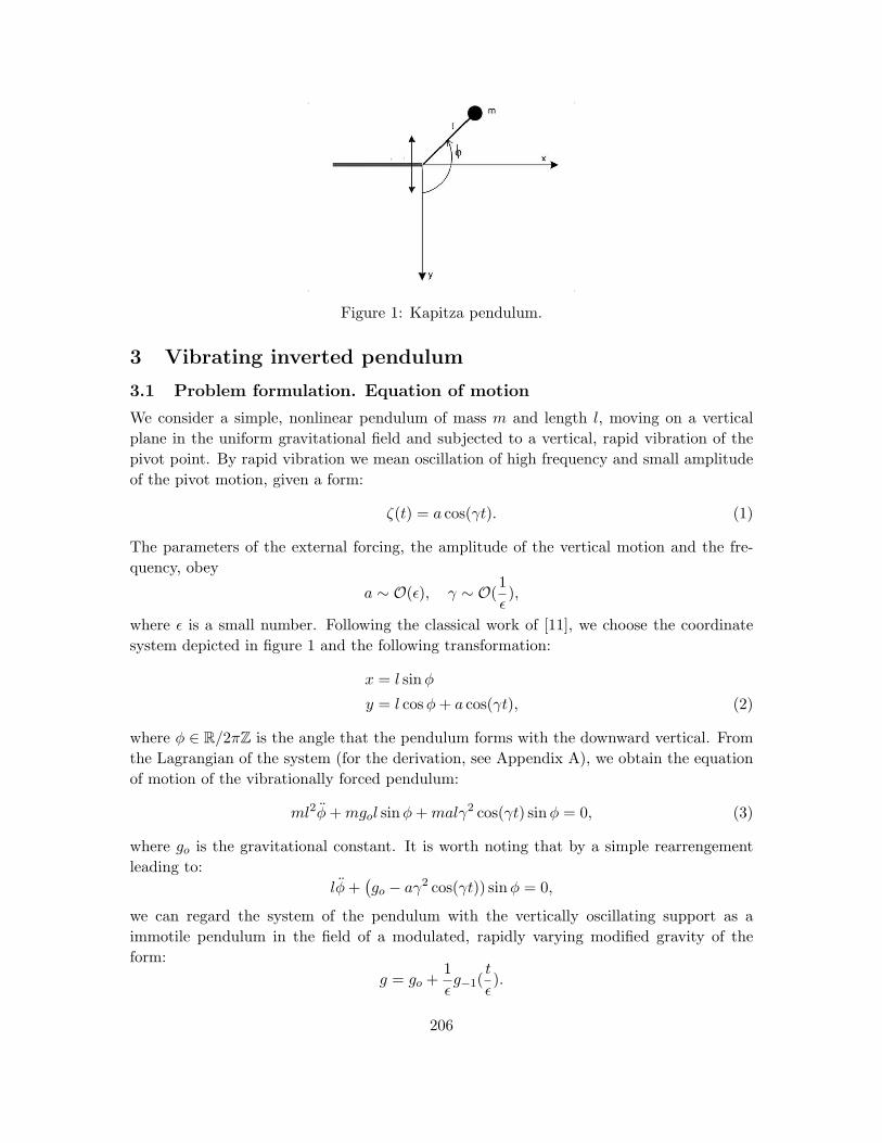
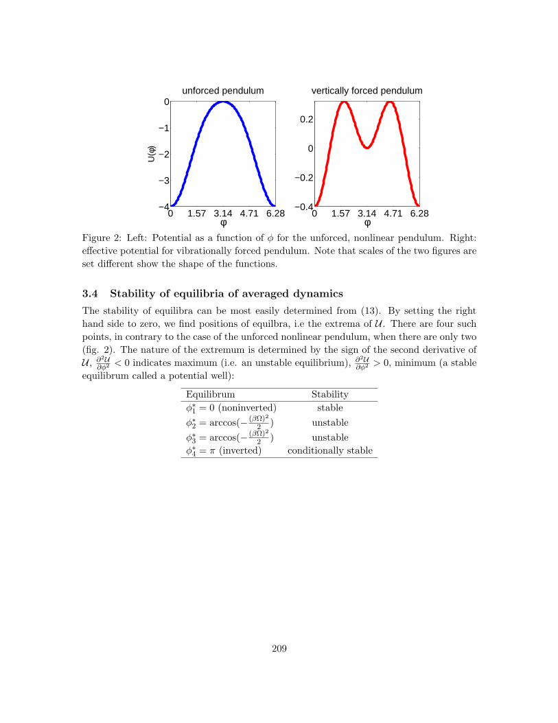
Figure 2: Left: Potential as a function of φ for the unforced, nonlinear pendulum. Right:effective potential for vibrationally forced pendulum. Note that scales of the two figures areset different show the shape of the functions.
3.4 Stability of equilibria of averaged dynamics
The stability of equilibra can be most easily determined from (13). By setting the righthand side to zero, we find positions of equilbra, i.e the extrema of U . There are four suchpoints, in contrary to the case of the unforced nonlinear pendulum, when there are only two(fig. 2). The nature of the extremum is determined by the sign of the second derivative ofU , ∂2U
∂φ2 < 0 indicates maximum (i.e. an unstable equilibrium), ∂2U∂φ2 > 0, minimum (a stable
equilibrum called a potential well):
Equilibrum Stabilityφ∗1 = 0 (noninverted) stableφ∗2 = arccos(− (βΩ)2
2 ) unstableφ∗3 = arccos(− (βΩ)2
2 ) unstableφ∗4 = π (inverted) conditionally stable
209
0 50 100−6
−4
−2
0
2
4
6
φ
3.05 3.1 3.15 3.2
−0.1
0
0.1
0.2
φ
d φ
/dt
0 50 100−6
−4
−2
0
2
4
6
φ
−2 0 2
−2
−1
0
1
2
φ
d φ
/dt
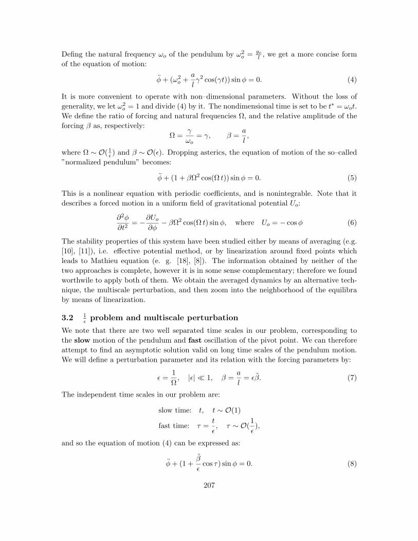
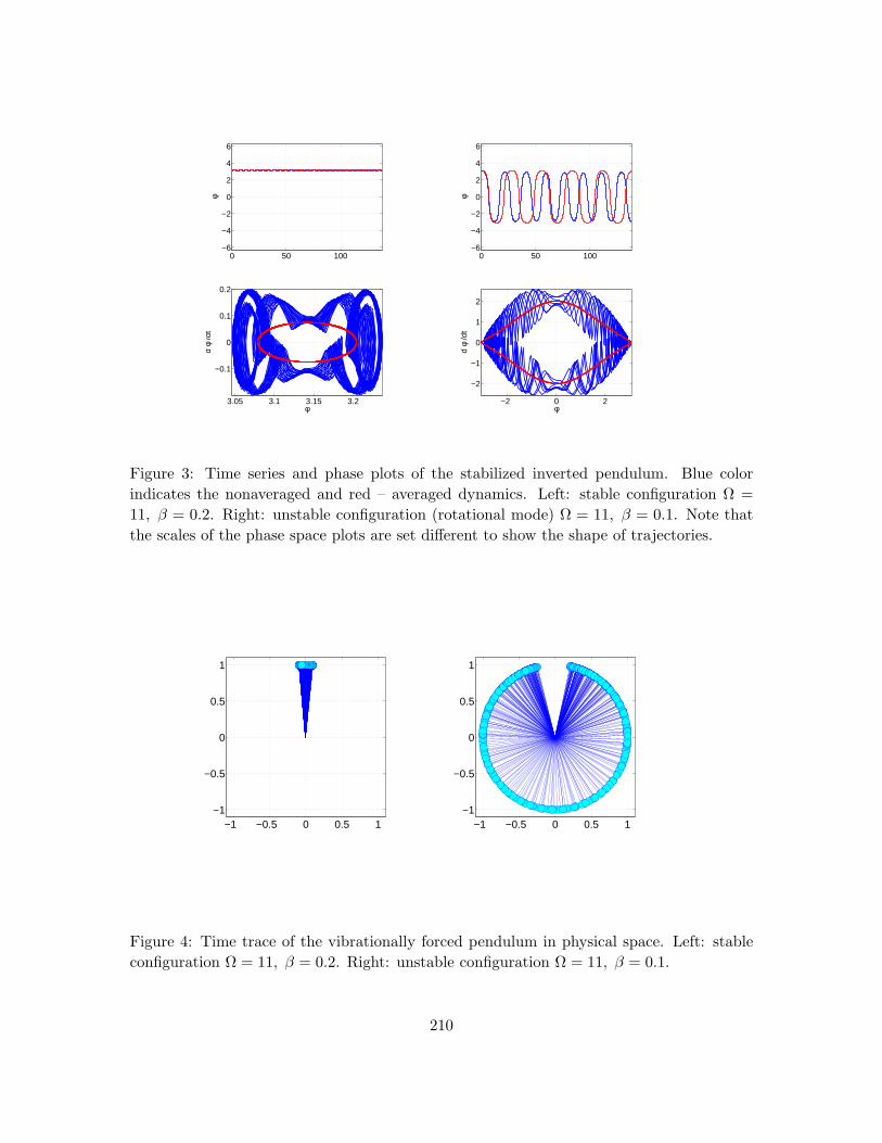
Figure 3: Time series and phase plots of the stabilized inverted pendulum. Blue colorindicates the nonaveraged and red – averaged dynamics. Left: stable configuration Ω =11, β = 0.2. Right: unstable configuration (rotational mode) Ω = 11, β = 0.1. Note thatthe scales of the phase space plots are set different to show the shape of trajectories.
−1 −0.5 0 0.5 1−1
−0.5
0
0.5
1
−1 −0.5 0 0.5 1−1
−0.5
0
0.5
1
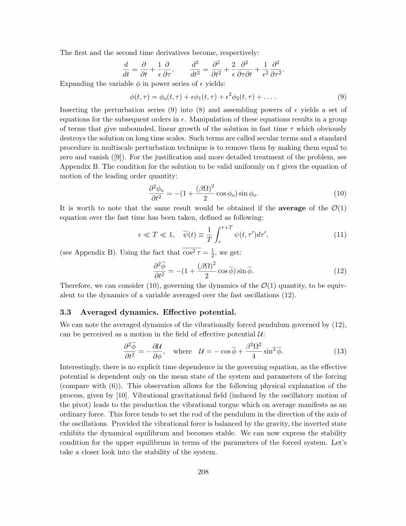
Figure 4: Time trace of the vibrationally forced pendulum in physical space. Left: stableconfiguration Ω = 11, β = 0.2. Right: unstable configuration Ω = 11, β = 0.1.
210
From (13), the condition for the stable upper equalibrum φ∗4 is:
β2Ω2
2> 1. (14)
The stability of the inverted position depends solely on the parameters of the system andrequires a forcing of suitably high frequency. Note also that an angle φ∗2,3 = arccos(− (βΩ)2
2 )can be interpreted as a width of the potential well, namely maximum initial displacementthat allows for the stabilization of the upper equilibrum for given properties of the forcing.Exemplary time series and phaseplots of the pendulum in a stable and unstable regimeis presented on figure 3, for both nonaveraged and averaged dynamics. Correspondingbehavior of the pendulum in the physical space is shown in figure 4.
There is another point of view of the averaged dynamics. The problem of the invert-ible pendulum may be considered in the 11
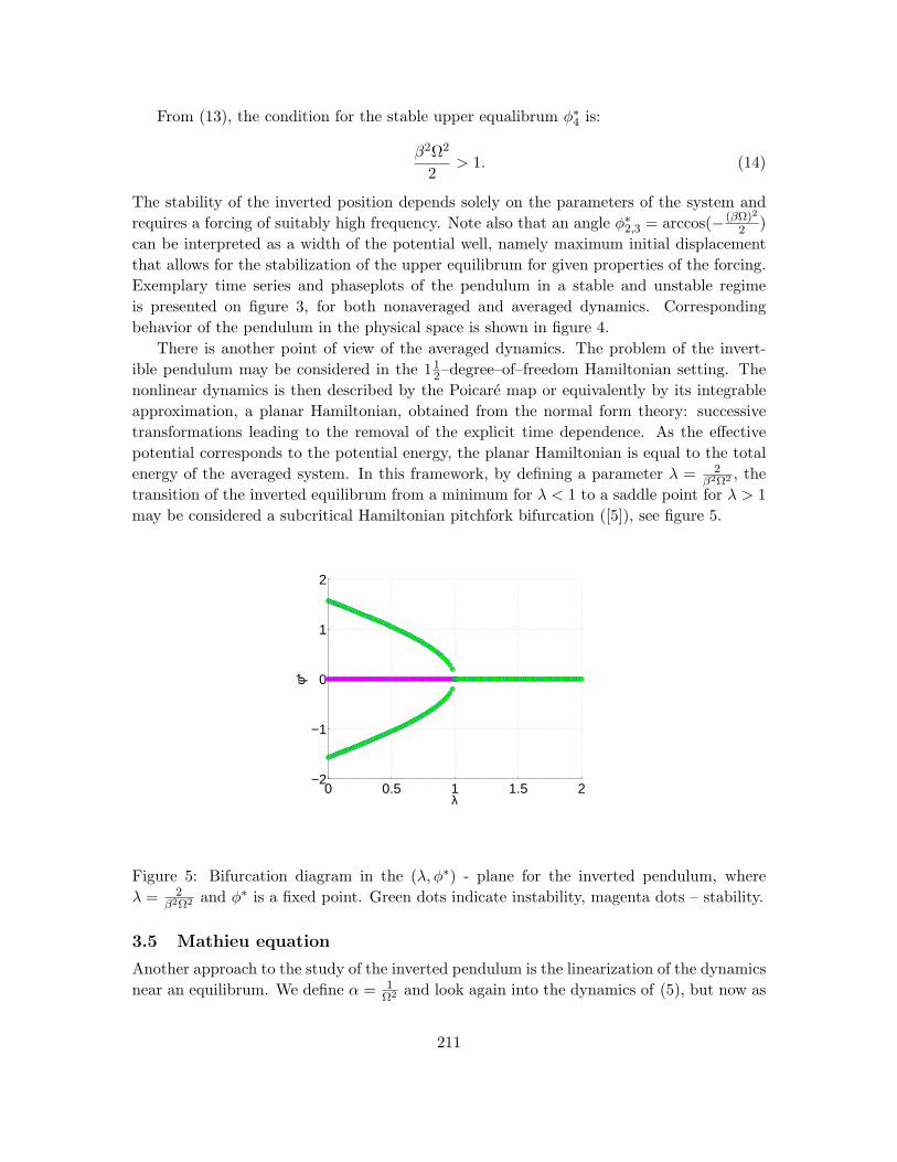
2–degree–of–freedom Hamiltonian setting. Thenonlinear dynamics is then described by the Poicare map or equivalently by its integrableapproximation, a planar Hamiltonian, obtained from the normal form theory: successivetransformations leading to the removal of the explicit time dependence. As the effectivepotential corresponds to the potential energy, the planar Hamiltonian is equal to the totalenergy of the averaged system. In this framework, by defining a parameter λ = 2
β2Ω2 , thetransition of the inverted equilibrum from a minimum for λ < 1 to a saddle point for λ > 1may be considered a subcritical Hamiltonian pitchfork bifurcation ([5]), see figure 5.
0 0.5 1 1.5 2−2
−1
0
1
2
φ*
λ
Figure 5: Bifurcation diagram in the (λ, φ∗) - plane for the inverted pendulum, whereλ = 2
β2Ω2 and φ∗ is a fixed point. Green dots indicate instability, magenta dots – stability.
3.5 Mathieu equation
Another approach to the study of the inverted pendulum is the linearization of the dynamicsnear an equilibrum. We define α = 1
Ω2 and look again into the dynamics of (5), but now as
211
evolving in the fast time τ = γt:
φττ + (α+ β cos τ) sinφ = 0. (15)
Now we zoom into the dynamics near π, so it is convenient to define the complementaryangular displacement ϕ with respect to φ, ϕ = π − φ. This is the angular displacementfrom the upper equilibrum position. Then sinϕ = sin(π − φ) = + sinφ and ϕττ = −φττ .The governing equation becomes:
ϕττ − (α+ β cos τ) sinϕ = 0. (16)
The sign of β is not important as it corresponds to the instantenous amplitude of the pivotmotion around the center of the coordinate system, which can be postive or negative. Thesign of α, however, matters. We define the variable ψ as
ψ =
φ : angular displacement near the lower equilibrum
ϕ : angular displacement near the upper equilibrum
and linearize sinψ ∼ ψ, obtaining the canonical form of Mathieu equation:
∂2ψ
∂τ2+ (α+ β cos τ)ψ = 0. (17)
Thus equation (17) describes linearized dynamics around the either fixed point, dependingon the sign of α:
α > 0 : lower equilibrum α < 0 : upper equilibrum (18)
This specific formulation allows the investigation of the linear stability near the eitherequilibrum based on the general results for the Mathieu equation. It is also a manifestationof the fact that we can tackle the stability of the inverted state by changing the sign ofthe gravity g. The stability of the periodic solutions of the Mathieu equation, given by the
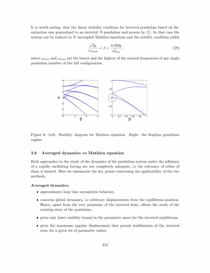
Floquet theory, can be determined from the diagram in (β, α) – parameter space ([9]). Theso–called transition curves separate regions of values α and β corresponding to unstable andstable solutions. Kapitza pendulum regime, with high forcing frequency (small α) and smallamplitude of the pivot motion (small β) lies in the region marked by the red circle in fig (6).The most surprising is the fact that, contrary to the averaged dynamics, linearized approachgives the possibility for destabilization of the lower equilibrum! We can obtain quite exactvalues for the parameter regions corresponding to stable inverted and noninverted equilibra:
Equilibrum Stability condition
inverted√
2Ω < β < 0.45 + 1.799
Ω2
noninverted 0 < β < 0.45− 1.799Ω2
212
It is worth noting, that the linear stability condition for inverted pendulum based on lin-earization was generalized to an inverted N -pendulum and proven by [1]. In that case thesystem can be reduces to N uncoupled Mathieu equations and the stabilty condition yields
√2g
γωmin< β <
0.450gω2
max
, (19)
where ωmin and ωmax are the lowest and the highest of the natural frequencies of any singlependulum member of the full configuration.
0 2 4 6−6
−4
−2
0
2
4
6
β
α
0 0.2 0.4 0.6 0.8 1−1
−0.5
0
0.5
1
β
Figure 6: Left: Stability diagram for Mathieu equation. Right: the Kapitza pendulumregime.
3.6 Averaged dynamics vs Mathieu equation
Both approaches to the study of the dynamics of the pendulum system under the influenceof a rapidly oscillating forcing are not completely adequate, i.e the relevance of either ofthem is limited. Here we summarize the key points concerning the applicability of the twomethods.
Averaged dynamics:
• approximates long time asymptotic behavior,
• concerns global dynamics, i.e arbitrary displacements from the equilibrum position.Hence, apart from the very proximity of the inverted state, allows the study of therotating state of the pendulum,
• gives only lower stability bound in the parameter space for the inverted equilibrium,
• gives the maximum angular displacement that permit stabilization of the invertedstate for a given set of parameter values,
213
• predicts the stability of the lower equilibrum for all the values of the parameters,
• gives physical explanation for the dynamical stabilization phenomenon in terms of theeffective potential.
Certainly some subtle details in the pendulum dynamics are lost in the approximate averageanalysis, which refers only to the slow component of the motion. In this method oneintroduces an approximation with no control on the relevance of the discarded dynamics,except of the estimate of their magnitude in terms of ε. There is always a region in parameterspace where the averaging fails predicting unstable configuration – the region over the upperbound in case of the inverted state and the whole unstable region for the lower equilibrum,which can be found from the Mathieu equation.
Linearized theory:
• reduces the problem to the well-known Mathieu equation,
• applies only to the vicinity of the fixed points, i.e is valid only for small angulardisplacements from the equilibrum position,
• gives more precisely defined stability regions: lower and upper bounds on the param-eter values,
• admits the possibility for destabilization of the lower equilibrum and gives the rangeof parameter values for which it should be observed,
• does not provide with any physical explanation of the phenomenon.
In general, the applicability of the Mathieu equation is limited as in general the linearstability cannot be extended immediately to the full system. However, it gives correctresults for the zoomed view into the dynamics near the equilibra.
4 Kapitza pendulum in fluid systems
4.1 Kapitza pendulum vs fluid systems
As already mentioned, we can regard a pendulum with a vertically oscillating support asequivalent to a pendulum with a stationary support in a periodically varying gravity field.This observation allows to attempt at finding an analogy between the Kapitza pendulumand fluid systems acted upon by vibrating gravitational forces, and thus study the dynamicsof the latter by methods developed in the preceding sections. A similar analogy was alreadymentioned by Lord Rayleigh ([15]), who considered a phenomenon observed in the famousFaraday experiment: a surface wave instability in a vertically vibrated container filled withfluid, with the frequency close to resonance with the natural frequency of the system.From that time on the problem has been studied widely both analytically (e.g. [2], [12],[13]) and experimentally (e.g. [4]). The ”Kapitza regime” discussed here is different asthe forcing frequency is much higher then the natural one and it would not be trivial to
214
think of an experiment similar to that of Faraday. One can rather search for an idealizedphysical situation. We have chosen a simple fluid system described by Boussinesq equations,characterized by density stratification and related buoyancy force, which action, combinedwith that of gravity, provides the mechanism for inertial oscillations with bounded naturalfrequency.
4.2 Boussinesq equations. Problem formulation
We will study the dynamics of a incompressible, inviscid, stratified, hydrostatic, non–rotating fluid, governed by nonlinear Boussinesq equations (the momentum equations, con-tinuity and conservation of density), see e.g. [16]):
Du
Dt+
1ρ
∂p
∂x= 0 (20)
Dw
Dt+
1ρ
∂p
∂z= −gρ
ρ= b (21)
∂u
∂x+∂w
∂z= 0 (22)
Dρ
Dt= 0 (23)
Here t is time and u and w are the components of the nondivergent velocity field in horizon-tal (x) and vertical (z) directions in a Cartesian frame of reference. The positive z–directionis antiparallel to gravity. We will work in the (x, z) – plane, which implies that all charac-teristics of the system are uniform in y.
We consider a hydrostically balanced reference state upon which perturbations are to beimposed and make use of the Boussinesq approximation, which means that the density field,represented by ρ(x, z, t) = ρ+ρo(z)+∆ρ(x, z, t) = ρ
(1−S
(zH
))+∆ρ(x, z, t), satisfies ρ >>
ρo(z) >> ∆ρ. The mean fluid density ρ is a uniform costant. The density stratification isassumed to be linear and S is a stability parameter defined as:
S =
+1 stable stratification
−1 unstable stratification
The vertical extent of the domain is small compared to a density depth scale H = |1ρdρ0
dz |−1.
Pressure field p is assumed to be hydrostatically related. The joint effect of gravity anddensity stratification leads to a buoyancy force b in the vertical. The natural frequency ofthe system, so–called the Brunt–Vaisala frequency, is defined through N2(z) = −(g
ρdρo
dz ),
which is constant in case of linear stratification, and with notation used here N = gSH . We
will constraint us to the flows with periodic boundary conditions.Nondivergence of the velocity field allows to introduce a stream function ψ, such that
u = ψz and w = −ψx. In an infinite medium the Boussinesq equations are satisfied byplanar internal waves of the form ψ = Ψ cos(kx + mz) e−iωt (with horizontal and verticalwave numbers k and m and κ =
√k2 +m2), which obey the dispersion relation ω = ±N k
|κ| .In polar coordinates chosen so that k = κ cosα and m = κ sinα we have ω = ±N cosα. The
215
frequency is therefore a function of the angle that the wave vector makes with the vertical.The condition for progressive waves is therefore 0 ≤ ω ≤ N so N acts as the upper boundof internal wave frequencies, corresponding to entirely vertical flow (buoyancy oscillation)([3]).
Now we will embed the system in a modified gravity field, varying in vertical as g(t) =go + aγ2 cos(γt), where go is a gravitational costant, the amplitude of oscillatory motionsatisfies a << go, and the frequency of the oscillations γ is much higher then the Brunt–Vaisala frequency, that is γ >> N .
We will nondimensionalize the system as follows:
(x∗, z∗) =( xH,z
H
), t∗ =
t√Hgo
,
which results in the nondimensional components of the velocity:
(u∗, w∗) =( u√
goH,
w√goH
).
The nondimensional density and pressure fields are:
ρ∗(x, z, t) =(1− S
( zH
))+ ∆ρ∗(x, z, t), where ∆ρ∗ =
∆ρρ, and p∗ =
p
ρgoH,
which gives the nondimensional Brunt–Vaisala frequency N∗2 = S. By introducing thenondimensional parameters:
Ω =γHgo
, β =a
H,
the ratio of the forcing and natural frequencies and the relative magnitude of the forcing,respectively, we get
g∗(t) =g(t)go
= 1 + βΩ2 cos(Ωt∗). (24)
By dropping asterics, the nondimensional Boussinesq equations are:
Du
Dt+∂p
∂x= 0 (25)
Dw
Dt+∂p
∂z= −∆ρ(1 + βΩ2 cos(Ωt)
)(26)
∂u
∂x+∂w
∂z= 0 (27)
∂∆ρ∂t
+ u∂∆ρ∂x
+ w∂∆ρ∂z
− wS = 0 (28)
We can eliminate the pressure by focusing on the vorticity equation, which is:
Dq
Dt=
D
Dt
(∂u∂z− ∂w
∂x
)=∂∆ρ∂x
(1 + βΩ2 cos(Ωt)
). (29)
It is evident that the vibrating gravity field modifies the basic mechanism of the baro-clinic generation of vorticity. We will now investigate this phenomenon in detail, using themethods derived for the stabilized inverted pendulum.
216
4.3 Multiscale expansion
We can observe that, similarly to the case of the Kapitza pendulum discussed above, in ourBoussinesq problem we have two well separated time scales: the slow gravity oscillationsand the fast oscillation of the gravity field. Thus, an attempt to find an asymptotic solutionvalid on long time scales is justified. Analogously as for the pendulum, we can define aperturbation parameter by ε = 1
Ω , and we have β ∼ O(ε). The slow time is then t ∼ O(1),and the fast time τ = Ωt, τ ∼ O(1
ε ), compare with (7). The oscillating gravity field (24)can be expressed as g(t) = 1 + 1
ε g−1(τ). Unlike in the pendulum case, system variablesdepend now not only on time, but also on space, therefore we have for the first, the secondand material time derivatives, respectively:
∂
∂t→ ∂
∂t+
1ε
∂
∂τ,
∂2
∂t2→ ∂2
∂t2+
2ε
∂2
∂τ∂t+
1ε2
∂2
∂τ2,
D
Dt=
∂
∂t+ u
∂
∂x+ w
∂
∂z.
With the averaging operator defined as (11), the components of the velocity perturbationare expanded in perturbation series as:
u(x, z, t, τ) = uo(x, z, t) + u′o(x, z, t, τ) + ...
w(x, z, t, τ) = wo(x, z, t) + w′o(x, z, t, τ) + .... ,(30)
where (uo, wo) refer to the mean perturbation velocity, while (u′o, w′o) correspond to the
disturbance due to modified acceleration of the order O(1ε ); after time integration, we can
expect them to be of the order O(1), but as they came from the oscillatory motion, they willvanish when averaged over the fast time. We will define the mean substantial derivative:
D
Dt=
∂
∂t+ uo
∂
∂x+ wo
∂
∂z.
The density perturbation is expanded in ε as:
∆ρ(x, z, t, τ) = ∆ρo(x, z, t, τ) + ε∆ρ1(x, z, t, τ) + ... . (31)
Inserting the series (31) and (30) into the density equation (28), we get:
∂∆ρo
∂t+
1ε
∂∆ρo
∂τ+ ε
∂∆ρ1
∂t+∂∆ρ1
∂τ+ uo
∂∆ρo
∂x+ u′o
∂∆ρo
∂x+ uo
∂∆ρ1
∂x+ u′o
∂∆ρ1
∂x+
+ wo∂∆ρo
∂x+ w′
o
∂∆ρo
∂x+ wo
∂∆ρ1
∂x+ w′
o
∂∆ρ1
∂x− woS − w′
oS = 0, (32)
Gathering terms of the order O(1ε ) we conclude that ∆ρo = ∆ρo(x, z, t). In the order
of O(1), we will first average out the terms containing perturbation quantities ∆ρ1 and(u′o, w
′o), so that the remaining terms give an evolution equation for the mean density
perurbation:D ∆ρDt
− woS = 0. (33)
Subtraction of (33) from (32) results in an evolution equation for ∆ρ1:
∂∆ρ1
∂τ+ u′o
∂∆ρo
∂x+ w′
o
∂∆ρo
∂z− w′
oS = 0. (34)
217
Inserting the perturbation series (30) into (29), we get:
∂
∂t
(∂uo
∂z− ∂wo
∂x
)+
1ε
∂
∂τ
(∂u′o∂z
− ∂w′o
∂x
)+ uo
∂
∂x
(∂uo
∂z− ∂wo
∂x
)+ wo
∂
∂z
(∂uo
∂z− ∂wo
∂x
)+
+ uo∂
∂x
(∂u′o∂z
− ∂w′o
∂x
)+ wo
∂
∂z
(∂u′o∂z
− ∂w′o
∂x
)+ u′o
∂
∂x
(∂uo
∂z− ∂wo
∂x
)+ w′
o
∂
∂z
(∂uo
∂z− ∂wo
∂x
)+
+ u′o∂
∂x
(∂u′o∂z
− ∂w′o
∂x
)+ w′
o
∂
∂z
(∂u′o∂z
− ∂w′o
∂x
)=∂∆ρo
∂x+
1εg−1(τ)
∂∆ρo
∂x+ g−1(τ)
∂∆ρ1
∂x+ ε
∂∆ρ1
∂x.
Terms of the order O(1ε ) gather in the evolution equation for q′o:
∂q′o∂τ
=∂
∂τ
(∂u′o∂z
− ∂w′o∂x
)= g−1(τ)
∂∆ρo
∂x. (35)
By applying the averaging operation to the O(1) ensamble, terms containing products ofthe leading order and prime quantities are eliminated and the evolution equation for themean perturbation vorticity follows:
Dq
Dt=∂∆ρo
∂x+
(∂∆ρ1
∂xg−1(τ)
)−
(u′o∂q′o∂x
+ w′o∂q′o∂z
). (36)
We will use the fact that averaging is a linear operator so that from the continuity equation(28) to obtain:
∂uo
∂x+∂wo
∂z= 0, and
∂u′o∂x
+∂w′o∂z
= 0. (37)
To summarize, we have arrive at two separated sets of equations with no explicit timedependence: for averaged perturbation variables and those generated by the forcing of oursystem. By analogy to the Kapitza pendulum, a stable stratification corresponds to thestable equilibrium of the pendulum, while the unstable stratification – to the inverted state.Now we will analyze the response of the system to the instantenous density disturbance todetermine how the vertical oscillations of the gravity field influence stability properties ofthe system as a whole.
4.4 Stability of the vibrating Boussinesq system
4.4.1 Monochromatic wave disturbance in x direction
We will start with a perturbation of the mean state of the form:
∆ρ = %o cos(kx). (38)
Assuming a perturbation streamfunction of the form ψ′o = Ψ′o cos(kx), from (35) we have
u′o = 0 and w′o = w′o(x) = (∆ρo)xx
k2
∫g−1(τ ′)dτ ′. Therefore in the (35), the advection terms
cancel out yielding d∆ρ1
dτ = Sw′o and they vanish in the equations for the evolution of themean density perturbation (33) the mean vorticity perturbation (36) to give:
Dq
Dt=∂∆ρo
∂x
(1 +
S(βΩ)2
2),
D∆ρo
Dt= Swo. (39)
218
Manipulation of these expresions yields the evolution equation for the mean density pertur-bation:
D2∆ρDt2
+ S2∗∆ρ = 0, where S2
∗ = S +β2Ω2
2, (40)
is the new modified nondimensional frequency, expressed by means of the stability parameter(note that S2 = 1 irrespective of the initial stability). Thus we conclude that in case ofa stable initial stratification (S = 1), the stability is augmented, while in case of unstableinitial stratification there is a stabilizing effect of the vertically oscillating gravity field. Thestability condition in the initially unstable case is:
β2Ω2
2> 1, (41)
which is identical to the analogous condition for the inverted Kapitza pendulum (14). Infact, the equation (40) itself may be perceived as a linear analog of (12) – unintentionallylinearized by the dynamics itself. We can thus expect all the results obtained from theMathieu equation for the inverted pendulum to be valid in the problem discussed here.
Assuming the plane wave solution of the form ψ = ψo cos(kx − ωt), we obtain thedispersion relation for the internal waves supported by our system:
ω2 = S2∗ ,
which is equivalent to the dispersion relation of the buoyancy oscillation typical to theunforced Boussinesq system, with N replaced by S∗, i.e. the system is stabilized and thefrequency of the vertical oscillation is higher then the maximum frequency in the unforcedcase.
4.4.2 Monochromatic plane wave disturbance
In case the initial density perturbation has a form of the planar wave:
∆ρ = %o cos(kx+mz), (42)
the procedure is conducted analogously as in the previous case. Although u′o 6= 0, fromthe continuity equation (37) we have uo
∂∂x = wo
∂∂z = u′o
∂∂x = w′o
∂∂x = 0 leading to the
cancellation of the advection terms. Consequently, the multiscale technique and averagingleads to the following stability condition for the averaged system:
D2
Dt2( ∂2
∂x2+
∂2
∂z2
)∆ρ+ S2
∗( ∂2
∂x2
)∆ρ = 0, where S2
∗ = S +( k2
k2 +m2
)β2Ω2
2.
As before, we conclude that in case of a stable initial stratification the stability is ampli-fied, while in case of the unstable initial stratification, the vibrating gravity results in thestabilizing effect whenever: ( k2
k2 +m2
)β2Ω2
2> 1, (43)
219
which is equivalent to (41), except that now the orientation of the perturbation in space(i.e.
(k2
k2+m2
)), matters. The dispersion relation in this case is:
ω2 = S2∗
k2
k2 +m2. (44)
Again, the form of the dispersion relation is equivalent to the dispersion relation of theinternal gravity wave solutions to the unforced case, with N replaced by S∗. The effectof the vibrational gravity forcing depends not only on the values of the parameters of theforcing, but also on the angle of the wavevector k: for a given forcing properties, verticaldisturbances are more difficult to suppress.
4.4.3 Perturbation of an arbitrary form
If we allow the instantenous density disturbance to have an arbitrary form ∆ρ(x, z), theadvective terms in (33, 34) and (36) do not cancel out and the mean vorticity equationtakes a form of an integro–differential equation:
Dq
Dt=∂∆ρ∂x
+(∂∆ρ1
∂xg−1
)− J (ψ′,∇2ψ′). (45)
Without further assumptions, it is difficult to construct any meaningful stability condition.However, if we could represent ∆ρ in Fourier series and linearize in u′o, w
′o and ∆ρ, we can
get rid of the advective terms and obtain the following form of the mean vorticity equation:
Dq
Dt=
∞∑n=1
(∂∆ρo
∂x
)n
(1 +
( k2n
k2n +m2
n
)β2Ω2
2
), (46)
which shows the additive effect of any single perturbation wave component of the series tothe baroclinic generation of the mean vorticity, modified by the vibrating gravity in similarway as in the previous simpler cases. The corresponding stability condition for an unstableinitial stratification is:
β2Ω2
2
∞∑n=1
( k2n
k2n +m2
n
)> 1, (47)
so again we can see that provided the instantenous density perturbation can be given a formof the sum of waves, there is an analogy between the effect of the vibrational forcing on thestability of the system in case of the Kapitza pendulum and dynamics of a fluid describedby ideal Boussinesq equations, with a modification due to nonlocality of the problem: for agiven values of forcing parameters the stability is strongly affected by the direction of thepropagation of the density disturbance.
5 Summary and conclusions
In this work we considered the inverted pendulum with the vibrating support. The applica-tion of multiscale perturbation, leading to the averaged dynamics, as well as linearization,allowed us to study the stabilization phenomenon. Then we used the multiscale technique
220
and averaging to an incompressible, inviscid, linearly stratified, nonlinear Boussinesq systemin a periodic domain, subjected to rapidly oscillating gravity field. We have shown that,provided the instantenous density perturbation can be given a form of a wave or sum ofwaves, the stabilization mechanism induced by the vibrational forcing is analogous to thatexhibited by the Kapitza pendulum. However, the dynamics of the Boussinesq system ismore complicated, as it evolves not only in time, but also in space. The resulting stabilitycondition for the initially unstable configuration is modified: it requires not only suitablyhigh frequency and small amplitude of the vibrating motion – the direction of propagationof the density perturbation in the space also plays a role. In case of a disturbance of a gen-eral form it is difficult to draw the conclusions about the system stability without furtherassumptions.
The work presented here is not just an idealized, educative example that contributes tothe understanding of the instability phenomena. There are indeed real physical situationsthat permits the use of Boussinesq approximation with the forcing regime as prescribedhere, though certainly requiring adequate boundary conditions and generally more complexanalysis. As an example, we give convective phenomena in radially pulsating stars, treatedin ([14]) by means of linearization. The appeal of the multiscale perturbation and averagingmethods discussed here is that they provide the description of the global behavior of theaveraged variable, expected to be the one related to any observed quantity. This observationstrongly encourages the application of these methods in any future investigation of thestability mechanisms in more realistic and complex fluid systems forced parametrically.
6 Acknowledgements
I would like to thank to my summer supervisor Oliver Buhler for his patience and indis-pensable help with the project and to all the GFD faculty and fellows for a great summer.
References
[1] D. J. Acheson, A pendulum theorem., Proc. Roy. Soc. London, 443 (1993), pp. 239–245.
[2] T. N. Benjamin and F. Ursell, The stability of the plane free surface of a liquid invertical periodic motion., Proc. Roy. Soc. London, 225 (1954), pp. 505–515.
[3] O. Buhler, Wave–mean interaction theory. Lecture notes., Courant Institute of Math-ematical Sciences, New York University, New York, 2004.
[4] W. S. Edwards and S. Fauve, Patterns and quasi–patterns in the faraday experi-ment, J. Fluid Mech., 278 (1994), pp. 123–148.
[5] I. H. H. W. Broer and M. van Noort, A reversible bifurcation analysis of theinverted pendulum, Physica D, 112 (1998), pp. 50–63.
221
[6] J. A. Holyst and W. Wojciechowski, The effect of kapitza pendulum and pricependulum, Physica A, 324 (2003), pp. 388–395.
[7] S. R. I. Gilary, N. Moiseyev and S. Fishman, Trapping of particles by lasers: thequantum kapitza pendulum, J. Phys. A., 36 (2003), pp. 409–415.
[8] H. J. T. S. J. A. Blackburn and N. Gronbech-Jensen, Stability and hopf bifur-cations in an inverted pendulum., Am. J. Phys., 60 (10) (1992), pp. 903–908.
[9] D. W. Jordan and P. Smith, Nonlinear ordinary differential equations, OxfordUniversity Press Inc., New York, 1987.
[10] P. Kapitza, Dynamical stability of a pendulum when its point of suspension vibratesand Pendulum with a vibrating suspension. In Collected Papers of Kapitza, edited byD. Haar., Pergamon Press, 1965.
[11] L.D.Landau and E. Lifshitz, Course in Theoretrical Physics. Mechanics. Vol(1).Third Edition., Pergamon Press, Oxford, 1976.
[12] J. Miles, Nonlinear faraday resonance, 146 (1984), pp. 451–460.
[13] J. R. Ockendon and H. Ockendon, Resonant surface waves, J. Fluid Mech., 59(1973), pp. 397–413.
[14] A. P. Poyet and E. A. Spiegel, The onset of convection in a radially pulsatingstar, Astron. J, 84 (12) (1979), pp. 1918–1931.
[15] L. Rayleigh, On maintained oscillations, Phil. Mag., 15 (1883), pp. 229–235.
[16] R. Salmon, Lectures On Geophysical Fluid Dynamics, Oxford University Press, NewYork, 1998.
[17] A. Stephenson, On a new type of dynamical stability, Mem. Proc.Manch. Lit. Phil.Soc., 52 (8) (1908), pp. 1–10.
[18] , On induced stability, Phil. Mag., 15 (1908), pp. 233–236.
[19] , On induced stability, Phil. Mag., 17 (1909), pp. 765–766.
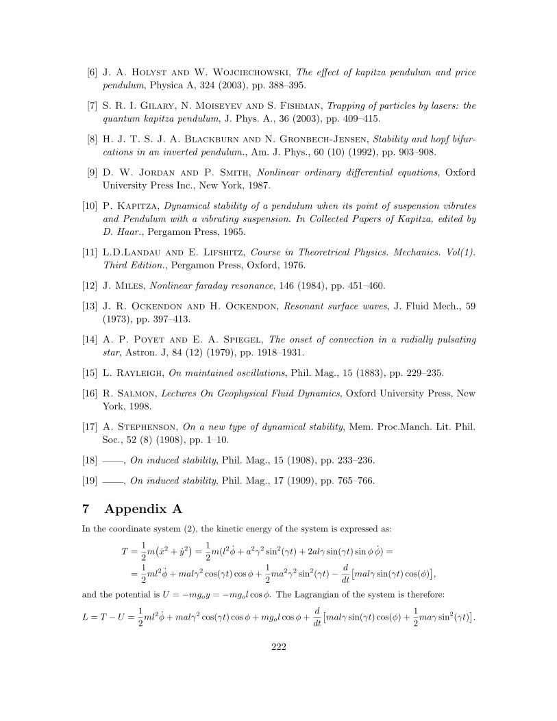
7 Appendix A
In the coordinate system (2), the kinetic energy of the system is expressed as:
T =12m
(x2 + y2
)=
12m(l2φ+ a2γ2 sin2(γt) + 2alγ sin(γt) sinφ φ) =
=12ml2φ+malγ2 cos(γt) cosφ+
12ma2γ2 sin2(γt)− d
dt
[malγ sin(γt) cos(φ)
],
and the potential is U = −mgoy = −mgol cosφ. The Lagrangian of the system is therefore:
L = T − U =12ml2φ+malγ2 cos(γt) cosφ+mgol cosφ+
d
dt
[malγ sin(γt) cos(φ) +
12maγ sin2(γt)
].
222
The complete time derivative on RHS does not enter the action, so from the Lagrange equation:
d
dt
(∂L
∂φ
)− ∂L
∂φ= 0,
we obtain the equation of motion of the vibrationally forced pendulum (3):
ml2φ+mgol sinφ+malγ2 cos(γt) sinφ = 0.
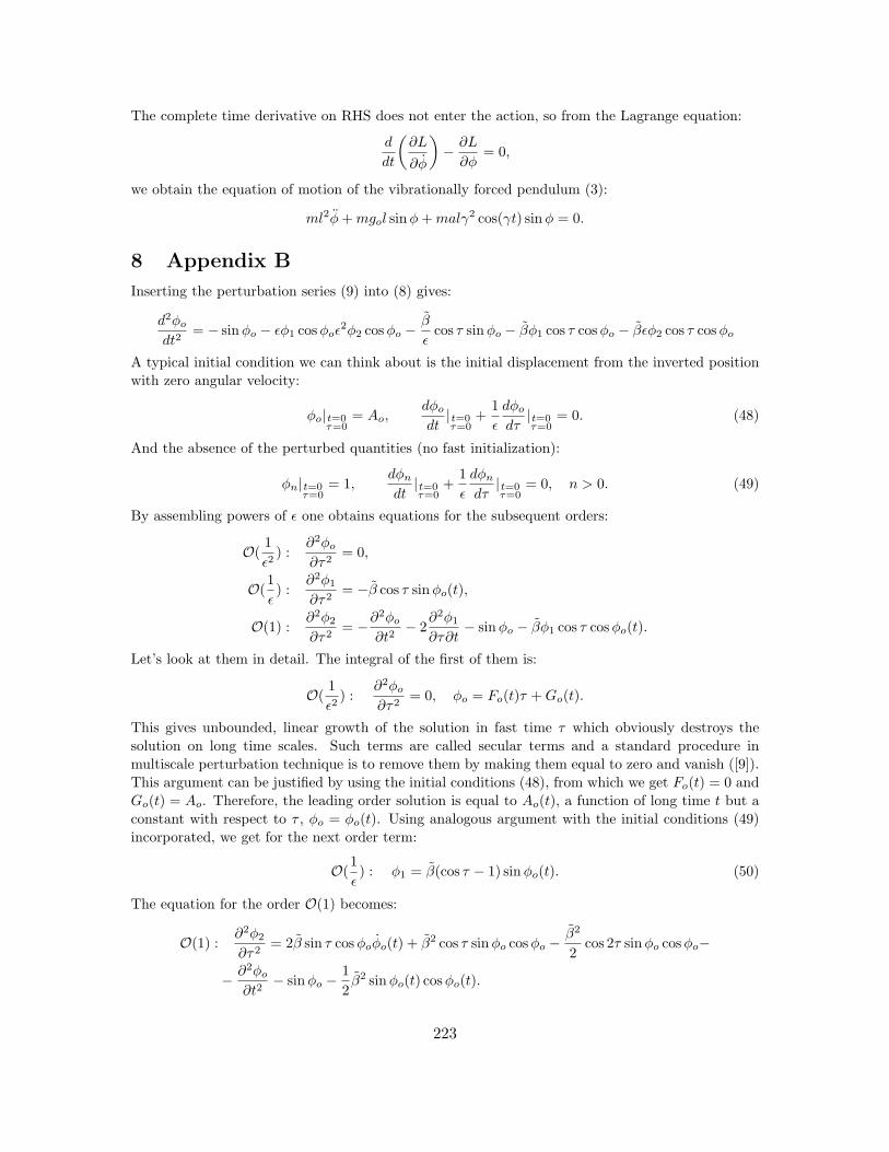
8 Appendix B
Inserting the perturbation series (9) into (8) gives:
d2φo
dt2= − sinφo − εφ1 cosφoε
2φ2 cosφo −β
εcos τ sinφo − βφ1 cos τ cosφo − βεφ2 cos τ cosφo
A typical initial condition we can think about is the initial displacement from the inverted positionwith zero angular velocity:
φo|t=0τ=0
= Ao,dφo
dt|t=0τ=0
+1ε
dφo
dτ|t=0τ=0
= 0. (48)
And the absence of the perturbed quantities (no fast initialization):
φn|t=0τ=0
= 1,dφn
dt|t=0τ=0
+1ε
dφn
dτ|t=0τ=0
= 0, n > 0. (49)
By assembling powers of ε one obtains equations for the subsequent orders:
O(1ε2
) :∂2φo
∂τ2= 0,
O(1ε) :
∂2φ1
∂τ2= −β cos τ sinφo(t),
O(1) :∂2φ2
∂τ2= −∂
2φo
∂t2− 2
∂2φ1
∂τ∂t− sinφo − βφ1 cos τ cosφo(t).
Let’s look at them in detail. The integral of the first of them is:
O(1ε2
) :∂2φo
∂τ2= 0, φo = Fo(t)τ +Go(t).
This gives unbounded, linear growth of the solution in fast time τ which obviously destroys thesolution on long time scales. Such terms are called secular terms and a standard procedure inmultiscale perturbation technique is to remove them by making them equal to zero and vanish ([9]).This argument can be justified by using the initial conditions (48), from which we get Fo(t) = 0 andGo(t) = Ao. Therefore, the leading order solution is equal to Ao(t), a function of long time t but aconstant with respect to τ , φo = φo(t). Using analogous argument with the initial conditions (49)incorporated, we get for the next order term:
O(1ε) : φ1 = β(cos τ − 1) sinφo(t). (50)
The equation for the order O(1) becomes:
O(1) :∂2φ2
∂τ2= 2β sin τ cosφoφo(t) + β2 cos τ sinφo cosφo −
β2
2cos 2τ sinφo cosφo−
− ∂2φo
∂t2− sinφo −
12β2 sinφo(t) cosφo(t).
223

Terms that are constants with respect to the fast time τ are a potential source for a secular growthin our solution. The condition for the solution to be valid uniformly on t gives the equation ofmotion of the leading order quantity (10). Note also that by taking the average defined by (11) ofthe equation (50), one gets (12).
224