video coding on multicore graphics processors (gpus) · video coding on multicore graphics...
TRANSCRIPT
Video coding on multicore graphics processors (GPUs)
Bruno Alexandre de Medeiros
Dissertation submitted to obtain the Master Degree inInformation Systems and Computer Engineering
JuryPresident: Doutor Joao Antonio Madeiras PereiraSupervisor: Doutor Nuno Filipe Valentim RomaVogal: Doutor David Manuel Martins de Matos
November 2012


Acknowledgments
I would like to thank to my supervisor, Dr Nuno Roma for his assistance, guidance and avail-
ability for providing the required help throughout this thesis.

Abstract
H.264/AVC is a recent video standard embraced by many multimedia applications. Because
of its demanding encoding requirements, a high amount of computational effort is often needed
in order to compress a video stream in real time. The intra-prediction and encoding are two of
several modules included by H.264 that requires a high computational power. On the other hand,
the GPU computational capabilities are exhibiting their supremacy for solving certain types of
problems with data parallelism, which composes the majority of the intra-prediction and encoding
process.
This dissertation presents a parallel implementation of the intra-prediction and encoding mod-
ules by adopting a parallel programming API denoted by CUDA, which explores the massive
parallelization capabilities of recent NVIDIA graphic cards in order to reduce the encoding time.
The developed solution is integrated in an existing encoder, where the intra-prediction and the
respective encoding are processed sequentially. The result of several conducted tests demon-
strates that the developed module is capable to speed up the sequential execution beyond the
computing capabilities of a recent CPU 1.
Keywords
H.264/AVC, Intra-prediction, Encoding, Parallelism, Performance, CUDA
1In this work, a recent CPU denotes a CPU introduced into the market between 2010 and 2012
iii

Resumo
O H.264/AVC e um standard de vıdeo adoptado por grande parte das aplicacoes de mul-
timedia. Devido a exigencia dos seus requisitos para a codificacao, uma grande processamento
e muitas vezes necessaria a fim de comprimir uma sequencia de vıdeo em tempo real. A predicao
intra e a codificacao sao dois de varios modulos que fazem parte do H.264 e que requerem um
elevado poder de computacao. Por outro lado, a capacidade de computacao das GPUs esta
a demonstrar a sua supremacia para resolver certos tipos de problemas com recurso ao par-
alelismo de dados, nos quais fazem parte a predicao intra e o processo de codificacao.
Esta dissertacao apresenta uma implementacao paralela dos modulos de predicao intra e
de codificacao desenvolvida com recurso a uma API de programacao paralela denominada por
CUDA, que permite explorar as capacidades de paralelizacao massiva das recentes placas graficas
da Nvidia de forma a reduzir o tempo de codificacao. A solucao desenvolvida e integrada numa
aplicacao existente onde a predicao intra e a codificacao sao processadas sequencialmente.
Atraves do resultado de diversos testes, e demonstrado que a solucao desenvolvida e capaz
de acelerar a implementacao para alem da capacidade de processamento de um processador
recente2.
Palavras Chave
H.264/AVC, Predicao, Codificacao, Paralelismo, Desempenho, CUDA
2Neste trabalho, um processador recente refere-se a qualquer processador introduzido no mercado entre 2010 e 2012
v

Contents
1 Introduction 2
1.1 Motivation . . . . . . . . . . . . . . . . . . . . . . . . . . . . . . . . . . . . . . . . . 3
1.2 Objectives . . . . . . . . . . . . . . . . . . . . . . . . . . . . . . . . . . . . . . . . . 3
1.3 Main Contributions . . . . . . . . . . . . . . . . . . . . . . . . . . . . . . . . . . . . 4
1.4 Dissertation outline . . . . . . . . . . . . . . . . . . . . . . . . . . . . . . . . . . . . 4
2 MPEG-4 Part 10/H.264 5
2.1 MPEG-4 Part 10/AVC standard . . . . . . . . . . . . . . . . . . . . . . . . . . . . . 6
2.2 Image Representation . . . . . . . . . . . . . . . . . . . . . . . . . . . . . . . . . . 7
2.2.1 Color Spaces . . . . . . . . . . . . . . . . . . . . . . . . . . . . . . . . . . . 8
2.3 Encoding Loop . . . . . . . . . . . . . . . . . . . . . . . . . . . . . . . . . . . . . . 9
2.4 Decoding Loop . . . . . . . . . . . . . . . . . . . . . . . . . . . . . . . . . . . . . . 10
2.5 Intra Prediction . . . . . . . . . . . . . . . . . . . . . . . . . . . . . . . . . . . . . . 10
2.5.1 4x4 Intra Prediction . . . . . . . . . . . . . . . . . . . . . . . . . . . . . . . 11
2.5.2 16x16 Intra Prediction . . . . . . . . . . . . . . . . . . . . . . . . . . . . . . 15
2.5.3 Intra 8x8 Chroma Prediction . . . . . . . . . . . . . . . . . . . . . . . . . . . 17
2.6 Transform Coding . . . . . . . . . . . . . . . . . . . . . . . . . . . . . . . . . . . . . 19
2.6.1 Transform Module . . . . . . . . . . . . . . . . . . . . . . . . . . . . . . . . 19
2.6.2 Quantization Module . . . . . . . . . . . . . . . . . . . . . . . . . . . . . . . 20
2.7 Profiles and Levels . . . . . . . . . . . . . . . . . . . . . . . . . . . . . . . . . . . . 21
3 Nvidia’s GPU Parallel Programming Platform 23
3.1 CUDA Programming Model . . . . . . . . . . . . . . . . . . . . . . . . . . . . . . . 24
3.1.1 CUDA Runtime . . . . . . . . . . . . . . . . . . . . . . . . . . . . . . . . . . 25
3.1.2 Memory Management . . . . . . . . . . . . . . . . . . . . . . . . . . . . . . 26
3.1.3 Concurrency, Communication and Synchronization . . . . . . . . . . . . . . 28
3.1.4 Compute Capabilities . . . . . . . . . . . . . . . . . . . . . . . . . . . . . . 29
3.1.5 Compilation Process . . . . . . . . . . . . . . . . . . . . . . . . . . . . . . . 29
3.2 Fermi GPU’s Architecture . . . . . . . . . . . . . . . . . . . . . . . . . . . . . . . . 31
3.2.1 Streaming Multiprocessor . . . . . . . . . . . . . . . . . . . . . . . . . . . . 32
vii
Contents
3.2.2 Memory Subsystem . . . . . . . . . . . . . . . . . . . . . . . . . . . . . . . 33
4 Related Work 39
4.1 Fast intra-prediction implementations based on General Purpose Processors (GPPs) 40
4.2 GPU implementation of H.264 Intra-Prediction . . . . . . . . . . . . . . . . . . . . 42
5 Solution Architecture 45
5.1 Problem Partitioning . . . . . . . . . . . . . . . . . . . . . . . . . . . . . . . . . . . 46
5.2 Requisites and Constraints . . . . . . . . . . . . . . . . . . . . . . . . . . . . . . . 49
5.3 Architecture Design . . . . . . . . . . . . . . . . . . . . . . . . . . . . . . . . . . . 50
5.3.1 Partitioning . . . . . . . . . . . . . . . . . . . . . . . . . . . . . . . . . . . . 51
5.3.2 Communication . . . . . . . . . . . . . . . . . . . . . . . . . . . . . . . . . . 55
5.3.3 Agglomeration . . . . . . . . . . . . . . . . . . . . . . . . . . . . . . . . . . 59
5.3.4 Mapping . . . . . . . . . . . . . . . . . . . . . . . . . . . . . . . . . . . . . . 64
5.4 Execution Model . . . . . . . . . . . . . . . . . . . . . . . . . . . . . . . . . . . . . 68
6 Implementation Process 73
6.1 Implemented Data Structures . . . . . . . . . . . . . . . . . . . . . . . . . . . . . . 74
6.2 Asynchronous Execution Model . . . . . . . . . . . . . . . . . . . . . . . . . . . . . 75
6.3 Optimizations . . . . . . . . . . . . . . . . . . . . . . . . . . . . . . . . . . . . . . . 75
7 Results 81
7.1 Performance Characterization . . . . . . . . . . . . . . . . . . . . . . . . . . . . . . 82
7.2 Testing Hardware . . . . . . . . . . . . . . . . . . . . . . . . . . . . . . . . . . . . . 82
7.3 Performance . . . . . . . . . . . . . . . . . . . . . . . . . . . . . . . . . . . . . . . 83
7.4 Analysis of Scalability . . . . . . . . . . . . . . . . . . . . . . . . . . . . . . . . . . 89
7.5 Discussion . . . . . . . . . . . . . . . . . . . . . . . . . . . . . . . . . . . . . . . . 90
8 Conclusions and Future Work 91
8.1 Conclusions . . . . . . . . . . . . . . . . . . . . . . . . . . . . . . . . . . . . . . . . 92
8.2 Future Work . . . . . . . . . . . . . . . . . . . . . . . . . . . . . . . . . . . . . . . . 93
A Appendix A 97
viii
List of Figures
2.1 Scope of video encoder standardization. . . . . . . . . . . . . . . . . . . . . . . . . 6
2.2 Structure of H.264/AVC video encoder. . . . . . . . . . . . . . . . . . . . . . . . . . 6
2.3 Spatial and temporal sampling of a video sequence. . . . . . . . . . . . . . . . . . 7
2.4 YCbCr sampling patterns . . . . . . . . . . . . . . . . . . . . . . . . . . . . . . . . 8
2.5 H.264/AVC encoding scheme. . . . . . . . . . . . . . . . . . . . . . . . . . . . . . . 9
2.6 Raster scan order of macroblocks. . . . . . . . . . . . . . . . . . . . . . . . . . . . 10
2.7 Selection of samples from neighbouring blocks. . . . . . . . . . . . . . . . . . . . . 11
2.8 4x4 Intra prediction modes. . . . . . . . . . . . . . . . . . . . . . . . . . . . . . . . 12
2.9 Encoding order of 4x4 blocks within a macroblock. . . . . . . . . . . . . . . . . . . 13
2.10 Intra prediction 16x16 modes. . . . . . . . . . . . . . . . . . . . . . . . . . . . . . . 16
2.11 DC mode. . . . . . . . . . . . . . . . . . . . . . . . . . . . . . . . . . . . . . . . . . 18
2.12 Result of a 2D DCT function. . . . . . . . . . . . . . . . . . . . . . . . . . . . . . . 20
3.1 Differences between CPU and GPU architectures. . . . . . . . . . . . . . . . . . . 24
3.2 Asynchronous timeline. . . . . . . . . . . . . . . . . . . . . . . . . . . . . . . . . . 25
3.3 Example of a grid organization using 2D coordinates. . . . . . . . . . . . . . . . . 26
3.4 Example of a serial and a CUDA parallel function that adds two arrays of size N. . 26
3.5 Example of an host and CUDA compilation workflow on an Unix machine. . . . . . 30
3.6 Architecture of a recent NVIDIA GPU. . . . . . . . . . . . . . . . . . . . . . . . . . 31
3.7 Fermi Streaming Multiprocessor (SM) . . . . . . . . . . . . . . . . . . . . . . . . . 33
3.8 Global memory coalescing. . . . . . . . . . . . . . . . . . . . . . . . . . . . . . . . 35
3.9 Example of an 128 bytes request by a warp to the global memory. . . . . . . . . . 36
3.10 Conflicting Share Memory access. . . . . . . . . . . . . . . . . . . . . . . . . . . . 37
4.1 Encoding decision based on a smoothness classification. . . . . . . . . . . . . . . 41
4.2 Flowchart of fast mode decision algorithm for intra prediction in H.264/AVC. . . . . 41
4.3 Execution sequence of intra predictions . . . . . . . . . . . . . . . . . . . . . . . . 42
4.4 Rearrangement of 4x4 block encoding order . . . . . . . . . . . . . . . . . . . . . . 43
4.5 Dependency between four 4x4 blocks . . . . . . . . . . . . . . . . . . . . . . . . . 43
ix
List of Figures
5.1 Dependency map between decomposed data structures. . . . . . . . . . . . . . . 52
5.2 Different granularities of decomposed tasks. . . . . . . . . . . . . . . . . . . . . . . 54
5.3 Data sharing of the intra-prediction and coding procedures on a macroblock. . . . 58
5.4 Example of a parallel reduction . . . . . . . . . . . . . . . . . . . . . . . . . . . . . 59
5.5 Agglomeration of the luminance’s 16x16 tasks. . . . . . . . . . . . . . . . . . . . . 61
5.6 Agglomeration of the luminance’s 4x4 tasks. . . . . . . . . . . . . . . . . . . . . . . 61
5.7 Dependencies and reordering of luminance 4x4 tasks. . . . . . . . . . . . . . . . . 62
5.8 Requisites of macroblocks’ dependencies. . . . . . . . . . . . . . . . . . . . . . . . 63
5.9 Example of different execution orders using one or multiple macroblocks. . . . . . 63
5.10 Example of an agglomeration composed by macroblocks from four intra-frames. . 65
5.11 Mapping of decomposed data elements and tasks to execution units. . . . . . . . . 66
5.12 Execution order of tasks that execute on the CPU and GPU. . . . . . . . . . . . . . 69
5.13 Overlap of memory operations with kernel executions. . . . . . . . . . . . . . . . . 69
5.14 Examples of sequential and pipelined execution with the CPU and GPU. . . . . . . 70
6.1 Two divergent execution paths in a group of two warps. . . . . . . . . . . . . . . . 78
7.1 Intra-process time using CIF video-sequences. . . . . . . . . . . . . . . . . . . . . 84
7.2 Total performance gain with CIF video-sequences. . . . . . . . . . . . . . . . . . . 85
7.3 Intra-process time using 4CIF video-sequences. . . . . . . . . . . . . . . . . . . . 85
7.4 Total performance gain with 4CIF video-sequences. . . . . . . . . . . . . . . . . . 86
7.5 Intra-process time using 1080p video-sequences. . . . . . . . . . . . . . . . . . . . 86
7.6 Total performance gain with 1080p video-sequences. . . . . . . . . . . . . . . . . . 87
7.7 Intra-process time using 1080p video-sequences with the luma 4x4 prediction mode
disabled. . . . . . . . . . . . . . . . . . . . . . . . . . . . . . . . . . . . . . . . . . 87
7.8 Total performance gain with 1080p video-sequences with luma 4x4 disabled. . . . 88
7.9 Intra-process time using 2160p video-sequence. . . . . . . . . . . . . . . . . . . . 88
7.10 Total performance gain with 2160p video-sequences. . . . . . . . . . . . . . . . . . 89
7.11 Comparison between different video resolutions. . . . . . . . . . . . . . . . . . . . 89
x
List of Tables
2.1 Video frame formats. . . . . . . . . . . . . . . . . . . . . . . . . . . . . . . . . . . . 7
3.1 Cuda variable type qualifiers. . . . . . . . . . . . . . . . . . . . . . . . . . . . . . . 27
3.2 Compute capability features list. . . . . . . . . . . . . . . . . . . . . . . . . . . . . 29
3.3 Fermi’s memory characteristics . . . . . . . . . . . . . . . . . . . . . . . . . . . . . 34
5.1 Decomposed data structures and relation to tasks. . . . . . . . . . . . . . . . . . . 53
5.2 Association between decomposed data structures and tasks. . . . . . . . . . . . . 55
7.1 Specification of the computational resources used for conducting the tests. . . . . 82
A.1 Time consumed in the encoding of 64 CIF (352x288) frames. . . . . . . . . . . . . 98
A.2 Time consumed in the encoding of 64 4CIF (705x576) frames. . . . . . . . . . . . 98
A.3 Time consumed in the encoding of 64 1080p frames. . . . . . . . . . . . . . . . . . 99
A.4 Time consumed in the encoding of 64 1080p frames with luma 4x4 disabled. . . . 99
A.5 Time consumed in the encoding of 64 2160p frames. . . . . . . . . . . . . . . . . . 100
xi

List of Tables
xii
List of Tables
Acronyms
ALU Arithmetic Logic Unit
AoS Arrays of Structures
API Application Programming Interface
CIF Common Intermediate Format
CUDA Compute Unified Device Architecture
DCT Discret Cosine Transform
DMA Direct Memory Access
DVD Digital Versatile Disk
ECC Error Check and Correction
FPU Floating Point Unit
GDDR Graphics Double Data Rate
GPU Graphics Processing Unit
HD High Definition
HEVC High Efficiency Video Coding
ILP Instruction-Level Parallelism
JVT Joint Video Team
LRU Least Recently Used
MB macroblock
PSNR Peak Signal-to-Noise Ratio
PTX Parallel Thread Execution
RD Rate Distortion
SAD sum of absolute differences
SFU Special Function Unit
SD Standard Definition
SM Streaming-Multiprocessor
SoA Structures of Arrays
SP Streaming-Processor
UHD Ultra High Definition
1

1Introduction
Contents1.1 Motivation . . . . . . . . . . . . . . . . . . . . . . . . . . . . . . . . . . . . . . . 31.2 Objectives . . . . . . . . . . . . . . . . . . . . . . . . . . . . . . . . . . . . . . . 31.3 Main Contributions . . . . . . . . . . . . . . . . . . . . . . . . . . . . . . . . . . 41.4 Dissertation outline . . . . . . . . . . . . . . . . . . . . . . . . . . . . . . . . . . 4
2
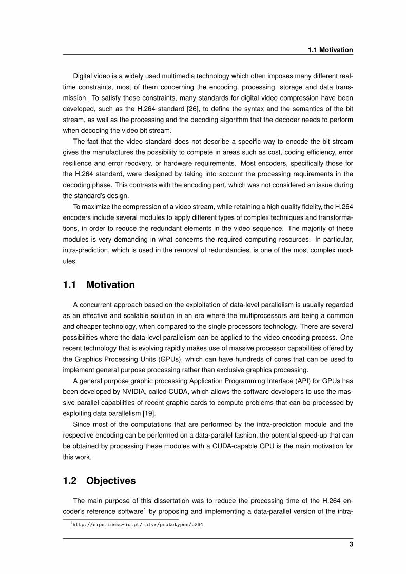
1.1 Motivation
Digital video is a widely used multimedia technology which often imposes many different real-
time constraints, most of them concerning the encoding, processing, storage and data trans-
mission. To satisfy these constraints, many standards for digital video compression have been
developed, such as the H.264 standard [26], to define the syntax and the semantics of the bit
stream, as well as the processing and the decoding algorithm that the decoder needs to perform
when decoding the video bit stream.
The fact that the video standard does not describe a specific way to encode the bit stream
gives the manufactures the possibility to compete in areas such as cost, coding efficiency, error
resilience and error recovery, or hardware requirements. Most encoders, specifically those for
the H.264 standard, were designed by taking into account the processing requirements in the
decoding phase. This contrasts with the encoding part, which was not considered an issue during
the standard’s design.
To maximize the compression of a video stream, while retaining a high quality fidelity, the H.264
encoders include several modules to apply different types of complex techniques and transforma-
tions, in order to reduce the redundant elements in the video sequence. The majority of these
modules is very demanding in what concerns the required computing resources. In particular,
intra-prediction, which is used in the removal of redundancies, is one of the most complex mod-
ules.
1.1 Motivation
A concurrent approach based on the exploitation of data-level parallelism is usually regarded
as an effective and scalable solution in an era where the multiprocessors are being a common
and cheaper technology, when compared to the single processors technology. There are several
possibilities where the data-level parallelism can be applied to the video encoding process. One
recent technology that is evolving rapidly makes use of massive processor capabilities offered by
the Graphics Processing Units (GPUs), which can have hundreds of cores that can be used to
implement general purpose processing rather than exclusive graphics processing.
A general purpose graphic processing Application Programming Interface (API) for GPUs has
been developed by NVIDIA, called CUDA, which allows the software developers to use the mas-
sive parallel capabilities of recent graphic cards to compute problems that can be processed by
exploiting data parallelism [19].
Since most of the computations that are performed by the intra-prediction module and the
respective encoding can be performed on a data-parallel fashion, the potential speed-up that can
be obtained by processing these modules with a CUDA-capable GPU is the main motivation for
this work.
1.2 Objectives
The main purpose of this dissertation was to reduce the processing time of the H.264 en-
coder’s reference software1 by proposing and implementing a data-parallel version of the intra-1http://sips.inesc-id.pt/~nfvr/prototypes/p264
3
1. Introduction
prediction and encoding modules. These parallel versions should be integrated into an existing
reference encoder software. During the execution time, and whenever a CUDA GPU is available,
the parallel module should replace the sequential implementation in order to offload the intra-
prediction and respective encoding tasks to the GPU. By assigning these tasks to the GPU, the
reference encoder can then proceed with other unrelated encoding tasks, which are concurrently
executed with the tasks on the GPU.
Besides offloading the intra-prediction and encoding tasks to the GPU, the developed imple-
mentation should also be as efficient as possible, in order to maximize the computing resources
available in the GPU, and present a scalable characteristic in order to adapt to different problem
sizes, such as the different video formats and spatial resolutions.
1.3 Main Contributions
The main contribution presented in this dissertation was the proposal and implementation of
the intra-prediction and encoding module, which was developed as a modular piece of software
that can be easily integrated into different encoders. As an example, besides the obvious ap-
plication to encode H.264 compressed video streams, this module may also be used to reduce
the compression time of multiple hyperspectral images, by processing all the images in a video
sequence with the intra-prediction and encoding module [32].
Besides the developed software, the conducted and presented analyses of the implementa-
tion, as well as the solution design can be used as a reference for developing or studying the
solution for similar problems, such as different video standards, different implementations or dif-
ferent modules in the H.264 with CUDA.
1.4 Dissertation outline
The proposed solution and the evaluation of its implementation are described in this work, as
well as the fundamental information required to better understand some of the described con-
cepts. The chapter 2 describes the fundamentals of the H.264 standard with an emphasis to the
intra-prediction and coding. The chapter 3 describes the CUDA API platform and the architecture
of a recent CUDA GPU2 . In chapter 4, it is described the related work regarding the implementa-
tion of the intra-prediction module in GPUs. The design of the implemented solution is described
in the chapter 5. In the chapter 6, it is specified the development process. In the chapter 7, it is
presented the conducted tests and analyses of the results. The chapter 8 outlines the conclusions
and the proposals for future work.
2A recent GPU denotes a GPU introduced into the marked in 2010.
4
2MPEG-4 Part 10/H.264
Contents2.1 MPEG-4 Part 10/AVC standard . . . . . . . . . . . . . . . . . . . . . . . . . . . . 62.2 Image Representation . . . . . . . . . . . . . . . . . . . . . . . . . . . . . . . . . 72.3 Encoding Loop . . . . . . . . . . . . . . . . . . . . . . . . . . . . . . . . . . . . . 92.4 Decoding Loop . . . . . . . . . . . . . . . . . . . . . . . . . . . . . . . . . . . . . 102.5 Intra Prediction . . . . . . . . . . . . . . . . . . . . . . . . . . . . . . . . . . . . 102.6 Transform Coding . . . . . . . . . . . . . . . . . . . . . . . . . . . . . . . . . . . 192.7 Profiles and Levels . . . . . . . . . . . . . . . . . . . . . . . . . . . . . . . . . . 21
5
2. MPEG-4 Part 10/H.264
This section describes some of the fundamental parts of the H.264 standard, with emphasis
in the intra-prediction module, which constitute the part on which this dissertation is focused.
2.1 MPEG-4 Part 10/AVC standard
The H.264 standard, also known as MPEG-4 part 10 Advanced Video Coding (AVC), is an
industry standard for video coding that appeared as a result of a joint research between the
ITU-T VCEG and the ISO/IEC MPEG standardization committee, established in December 2001
[26]. When compared with the other previous standards, it offers a substantial improvement in
coding efficiency and video quality. In fact, the main goal of this new standard was to enhance
the compression rate, while still providing a packed based video coding suitable for real-time
conversation, storage, and streaming or broadcast type applications.
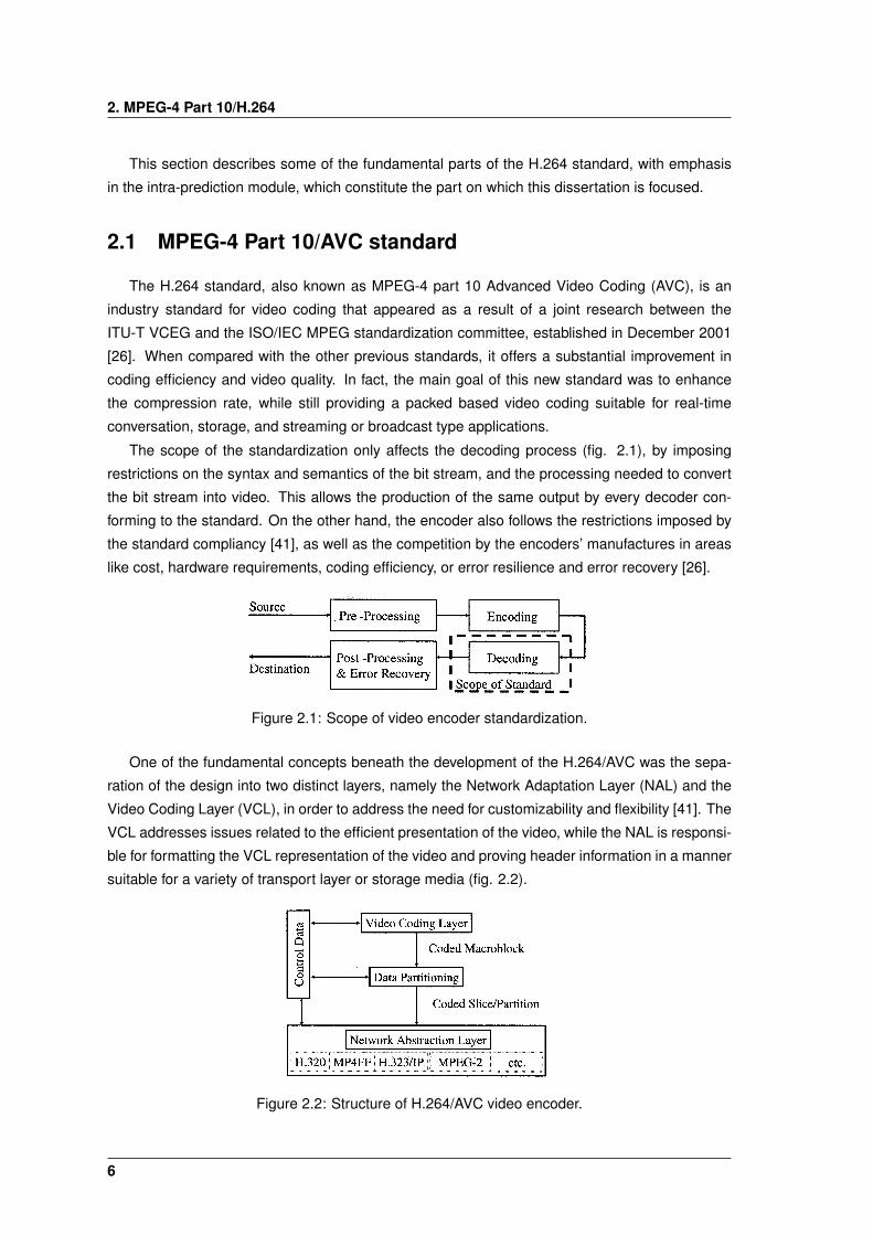
The scope of the standardization only affects the decoding process (fig. 2.1), by imposing
restrictions on the syntax and semantics of the bit stream, and the processing needed to convert
the bit stream into video. This allows the production of the same output by every decoder con-
forming to the standard. On the other hand, the encoder also follows the restrictions imposed by
the standard compliancy [41], as well as the competition by the encoders’ manufactures in areas
like cost, hardware requirements, coding efficiency, or error resilience and error recovery [26].
Figure 2.1: Scope of video encoder standardization.
One of the fundamental concepts beneath the development of the H.264/AVC was the sepa-
ration of the design into two distinct layers, namely the Network Adaptation Layer (NAL) and the
Video Coding Layer (VCL), in order to address the need for customizability and flexibility [41]. The
VCL addresses issues related to the efficient presentation of the video, while the NAL is responsi-
ble for formatting the VCL representation of the video and proving header information in a manner
suitable for a variety of transport layer or storage media (fig. 2.2).
Figure 2.2: Structure of H.264/AVC video encoder.
6

2.2 Image Representation
Standard DefinitionFormat Luminance resolution
(horiz. vs vert.)Sub-QCIF 128x96Quarter CIF (QCIF) 176x144CIF 352x2884CIF 704x576
High DefinitionFormat Luminance resolution
(horiz. vs vert.)720p 1280x7201080p 1920x10802160p 3840x21604320p 7680x4320
Table 2.1: Video frame formats.
2.2 Image Representation
Figure 2.3: Spatial and temporal sampling of a video sequence.
Digital video is formed by an ordered and discrete set of spatial and temporal samples of a
visual scene (see fig. 2.3). A frame is the result of a temporal sample from a video scene at a
given point of time. The moving video signal is produced by the repeated temporal sampling at
well defined intervals (e.g. 1/25 or 1/30 second intervals) [29]. A higher temporal sampling rate
(frame rate) produces a smooth apparent motion in the video scene, but requires more samples
to be captured and stored, and a higher data rate for video transmission. On the other side, a
lower frame rate reduces the number of captured and stored frames, as well a lower data rate for
transmission, but may produce unnatural motion in the video scene.
Conversely, the spatial sampling is formed by an array of intensity values at sample points
defined in a regular two-dimensional grid [1]. Each sample point is represented by a pixel in
the digitalized image. Coarser sample points produce a low-resolution sampled image whilst a
higher number of sampling points increases the resolution of the sampled image. The sample’s
resolution influences the volume of data to be stored or transmitted.
There are a wide variety of video frame formats. The most common formats are the Standard
Definition (SD) and the High Definition (HD) (see table 2.1). The Common Intermediate For-
mat (CIF) resolution is the basis for the Standard Definition formats, which ranges from the low
resolution Sub-QCIF to a higher resolution 4CIF. The High Definition video formats are having a
growing adoption from a variety of consumer products. Their resolutions ranges from the 720p
(HD) to the 4320p Ultra High Definition (UHD).
7
2. MPEG-4 Part 10/H.264
2.2.1 Color Spaces
Each pixel is a single picture element in a digital video image and stores the information about
its colour and luminance (or brightness) [35]. Colour video sequences require at least three values
per pixel to accurately represent colour (monochrome video sequences require just one value to
represent luminance). Two of the most widely used colour spaces are the RGB and the YCbCr.
In the RGB colour space, a colour image sample is represented by three primary colours with
the same resolution1: red (R), green (G) and blue (B). The combination of the intensity value of
these components gives the appearance of a ”true” colour.
Because the human visual system is more sensitive to luminance than to colour, the YCbCr
colour space (also known as YUV) allows a more efficient way to represent a colour image, by
separating the information regarding to the luminance from the colour information, and represent-
ing the colour with a lower resolution than luminance [28]. In the YUV colour space, the picture
information consists of the luminance (Y) plus two colour signals U (or Cb) and V (or Cr). The
conversion between the YUV and the RGB colour space [10] is defined by:YUV
=
0.299 0.587 0.114−0.146 −0.288 0.4340.617 −0.517 −0.100
×RGB
(2.1)
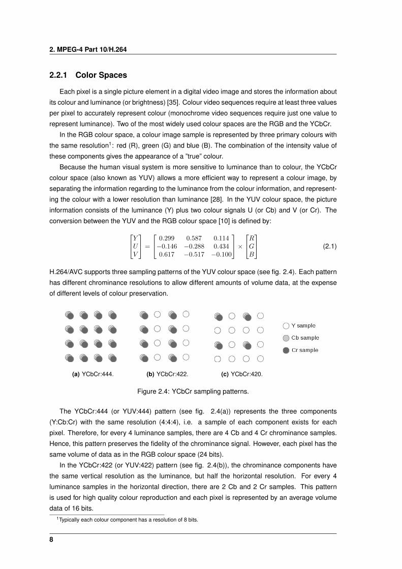
H.264/AVC supports three sampling patterns of the YUV colour space (see fig. 2.4). Each pattern
has different chrominance resolutions to allow different amounts of volume data, at the expense
of different levels of colour preservation.
(a) YCbCr:444. (b) YCbCr:422. (c) YCbCr:420.
Figure 2.4: YCbCr sampling patterns.
The YCbCr:444 (or YUV:444) pattern (see fig. 2.4(a)) represents the three components
(Y:Cb:Cr) with the same resolution (4:4:4), i.e. a sample of each component exists for each
pixel. Therefore, for every 4 luminance samples, there are 4 Cb and 4 Cr chrominance samples.
Hence, this pattern preserves the fidelity of the chrominance signal. However, each pixel has the
same volume of data as in the RGB colour space (24 bits).
In the YCbCr:422 (or YUV:422) pattern (see fig. 2.4(b)), the chrominance components have
the same vertical resolution as the luminance, but half the horizontal resolution. For every 4
luminance samples in the horizontal direction, there are 2 Cb and 2 Cr samples. This pattern
is used for high quality colour reproduction and each pixel is represented by an average volume
data of 16 bits.1Typically each colour component has a resolution of 8 bits.
8
2.3 Encoding Loop
The most common pattern is the YCbCr:420 (or YUV:420) (see fig. 2.4(c)). Each Cb and
Cr component has one half of the luminance’s horizontal and vertical resolution. This sampling
pattern is widely used for consumer applications, such as video conferencing, digital television
and Digital Versatile Disk (DVD) storage. Because each colour component has one quarter of
the number of samples in the luminance component, each pixel’s information is represented (as
average) with 12 bits. Hence, this pattern has the least preservation of the colour component
(among the previous two).
2.3 Encoding Loop
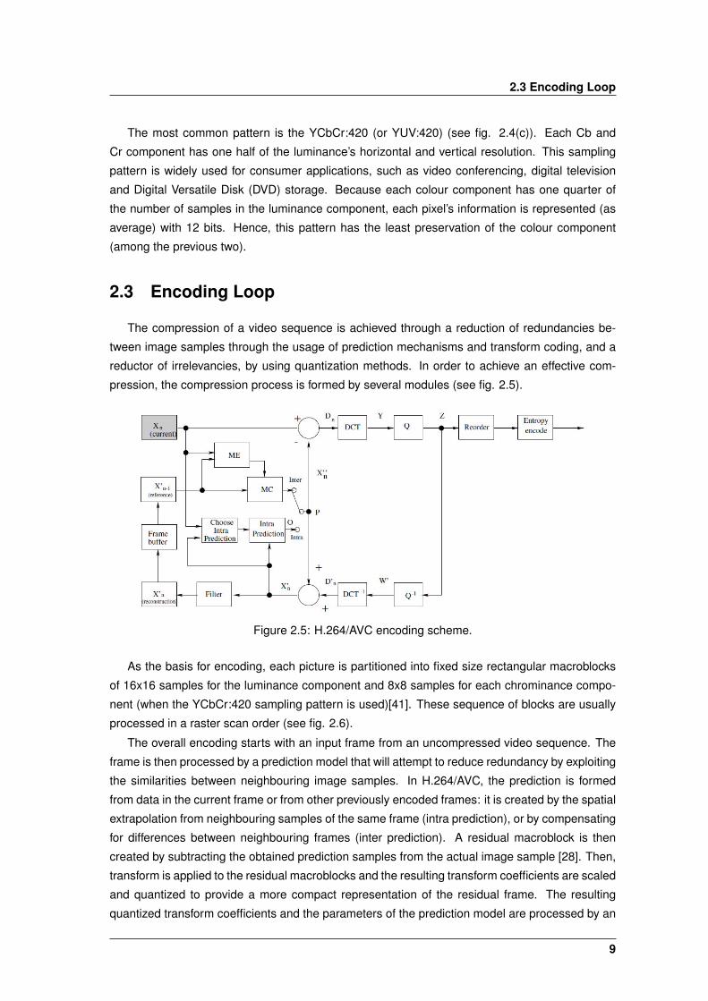
The compression of a video sequence is achieved through a reduction of redundancies be-
tween image samples through the usage of prediction mechanisms and transform coding, and a
reductor of irrelevancies, by using quantization methods. In order to achieve an effective com-
pression, the compression process is formed by several modules (see fig. 2.5).
Figure 2.5: H.264/AVC encoding scheme.
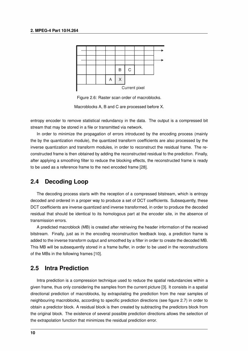
As the basis for encoding, each picture is partitioned into fixed size rectangular macroblocks
of 16x16 samples for the luminance component and 8x8 samples for each chrominance compo-
nent (when the YCbCr:420 sampling pattern is used)[41]. These sequence of blocks are usually
processed in a raster scan order (see fig. 2.6).
The overall encoding starts with an input frame from an uncompressed video sequence. The
frame is then processed by a prediction model that will attempt to reduce redundancy by exploiting
the similarities between neighbouring image samples. In H.264/AVC, the prediction is formed
from data in the current frame or from other previously encoded frames: it is created by the spatial
extrapolation from neighbouring samples of the same frame (intra prediction), or by compensating
for differences between neighbouring frames (inter prediction). A residual macroblock is then
created by subtracting the obtained prediction samples from the actual image sample [28]. Then,
transform is applied to the residual macroblocks and the resulting transform coefficients are scaled
and quantized to provide a more compact representation of the residual frame. The resulting
quantized transform coefficients and the parameters of the prediction model are processed by an
9
2. MPEG-4 Part 10/H.264
Figure 2.6: Raster scan order of macroblocks.
Macroblocks A, B and C are processed before X.
entropy encoder to remove statistical redundancy in the data. The output is a compressed bit
stream that may be stored in a file or transmitted via network.
In order to minimize the propagation of errors introduced by the encoding process (mainly
the by the quantization module), the quantized transform coefficients are also processed by the
inverse quantization and transform modules, in order to reconstruct the residual frame. The re-
constructed frame is then obtained by adding the reconstructed residual to the prediction. Finally,
after applying a smoothing filter to reduce the blocking effects, the reconstructed frame is ready
to be used as a reference frame to the next encoded frame [28].
2.4 Decoding Loop
The decoding process starts with the reception of a compressed bitstream, which is entropy
decoded and ordered in a proper way to produce a set of DCT coefficients. Subsequently, these
DCT coefficients are inverse quantized and inverse transformed, in order to produce the decoded
residual that should be identical to its homologous part at the encoder site, in the absence of
transmission errors.
A predicted macroblock (MB) is created after retrieving the header information of the received
bitstream. Finally, just as in the encoding reconstruction feedback loop, a prediction frame is
added to the inverse transform output and smoothed by a filter in order to create the decoded MB.
This MB will be subsequently stored in a frame buffer, in order to be used in the reconstructions
of the MBs in the following frames [10].
2.5 Intra Prediction
Intra prediction is a compression technique used to reduce the spatial redundancies within a
given frame, thus only considering the samples from the current picture [3]. It consists in a spatial
directional prediction of macroblocks, by extrapolating the prediction from the near samples of
neighbouring macroblocks, according to specific prediction directions (see figure 2.7) in order to
obtain a predictor block. A residual block is then created by subtracting the predictors block from
the original block. The existence of several possible prediction directions allows the selection of
the extrapolation function that minimizes the residual prediction error.
10
2.5 Intra Prediction
This intra prediction is applied separately to the luminance and chrominance samples. In
both color samples, the prediction is performed in the entire macroblock at once. The luminance
samples are also processed using the entire macroblock, but may be further refined using sixteen
4x4 blocks of a macroblock, for increasing the prediction effectiveness in samples with higher
detail. In this case, it is chosen the intra prediction mode with the lowest residual prediction error.
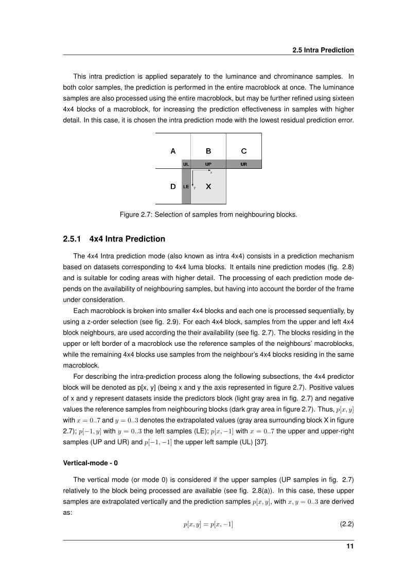
Figure 2.7: Selection of samples from neighbouring blocks.
2.5.1 4x4 Intra Prediction
The 4x4 Intra prediction mode (also known as intra 4x4) consists in a prediction mechanism
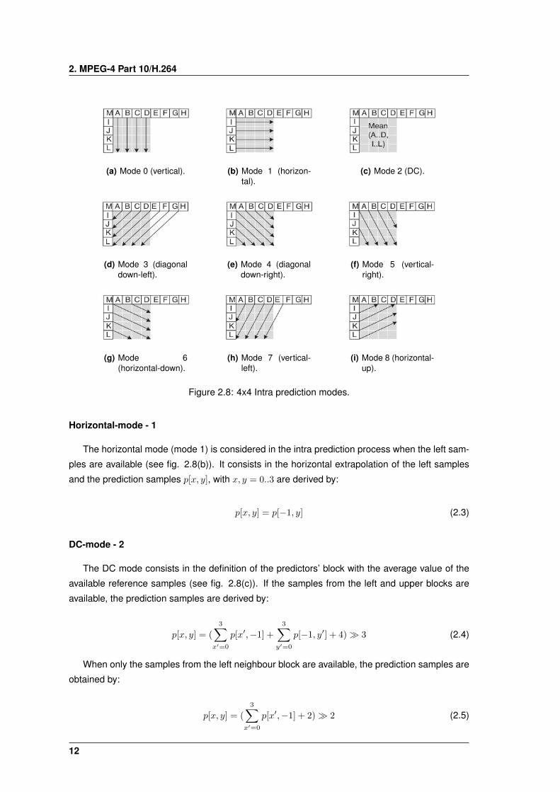
based on datasets corresponding to 4x4 luma blocks. It entails nine prediction modes (fig. 2.8)
and is suitable for coding areas with higher detail. The processing of each prediction mode de-
pends on the availability of neighbouring samples, but having into account the border of the frame
under consideration.
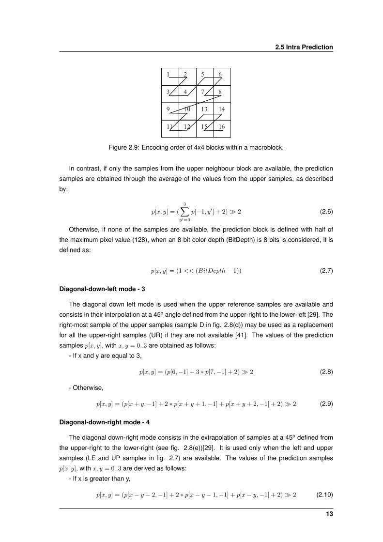
Each macroblock is broken into smaller 4x4 blocks and each one is processed sequentially, by
using a z-order selection (see fig. 2.9). For each 4x4 block, samples from the upper and left 4x4
block neighbours, are used according the their availability (see fig. 2.7). The blocks residing in the
upper or left border of a macroblock use the reference samples of the neighbours’ macroblocks,
while the remaining 4x4 blocks use samples from the neighbour’s 4x4 blocks residing in the same
macroblock.
For describing the intra-prediction process along the following subsections, the 4x4 predictor
block will be denoted as p[x, y] (being x and y the axis represented in figure 2.7). Positive values
of x and y represent datasets inside the predictors block (light gray area in fig. 2.7) and negative
values the reference samples from neighbouring blocks (dark gray area in figure 2.7). Thus, p[x, y]
with x = 0..7 and y = 0..3 denotes the extrapolated values (gray area surrounding block X in figure
2.7); p[−1, y] with y = 0..3 the left samples (LE); p[x,−1] with x = 0..7 the upper and upper-right
samples (UP and UR) and p[−1,−1] the upper left sample (UL) [37].
Vertical-mode - 0
The vertical mode (or mode 0) is considered if the upper samples (UP samples in fig. 2.7)
relatively to the block being processed are available (see fig. 2.8(a)). In this case, these upper
samples are extrapolated vertically and the prediction samples p[x, y], with x, y = 0..3 are derived
as:
p[x, y] = p[x,−1] (2.2)
11
2. MPEG-4 Part 10/H.264
(a) Mode 0 (vertical). (b) Mode 1 (horizon-tal).
(c) Mode 2 (DC).
(d) Mode 3 (diagonaldown-left).
(e) Mode 4 (diagonaldown-right).
(f) Mode 5 (vertical-right).
(g) Mode 6(horizontal-down).
(h) Mode 7 (vertical-left).
(i) Mode 8 (horizontal-up).
Figure 2.8: 4x4 Intra prediction modes.
Horizontal-mode - 1
The horizontal mode (mode 1) is considered in the intra prediction process when the left sam-
ples are available (see fig. 2.8(b)). It consists in the horizontal extrapolation of the left samples
and the prediction samples p[x, y], with x, y = 0..3 are derived by:
p[x, y] = p[−1, y] (2.3)
DC-mode - 2
The DC mode consists in the definition of the predictors’ block with the average value of the
available reference samples (see fig. 2.8(c)). If the samples from the left and upper blocks are
available, the prediction samples are derived by:
p[x, y] = (
3∑x′=0
p[x′,−1] +3∑
y′=0
p[−1, y′] + 4)� 3 (2.4)
When only the samples from the left neighbour block are available, the prediction samples are
obtained by:
p[x, y] = (
3∑x′=0
p[x′,−1] + 2)� 2 (2.5)
12
2.5 Intra Prediction
Figure 2.9: Encoding order of 4x4 blocks within a macroblock.
In contrast, if only the samples from the upper neighbour block are available, the prediction
samples are obtained through the average of the values from the upper samples, as described
by:
p[x, y] = (
3∑y′=0
p[−1, y′] + 2)� 2 (2.6)
Otherwise, if none of the samples are available, the prediction block is defined with half of
the maximum pixel value (128), when an 8-bit color depth (BitDepth) is 8 bits is considered, it is
defined as:
p[x, y] = (1 << (BitDepth− 1)) (2.7)
Diagonal-down-left mode - 3
The diagonal down left mode is used when the upper reference samples are available and
consists in their interpolation at a 45o angle defined from the upper-right to the lower-left [29]. The
right-most sample of the upper samples (sample D in fig. 2.8(d)) may be used as a replacement
for all the upper-right samples (UR) if they are not available [41]. The values of the prediction
samples p[x, y], with x, y = 0..3 are obtained as follows:
- If x and y are equal to 3,
p[x, y] = (p[6,−1] + 3 ∗ p[7,−1] + 2)� 2 (2.8)
- Otherwise,
p[x, y] = (p[x+ y,−1] + 2 ∗ p[x+ y + 1,−1] + p[x+ y + 2,−1] + 2)� 2 (2.9)
Diagonal-down-right mode - 4
The diagonal down-right mode consists in the extrapolation of samples at a 45o defined from
the upper-right to the lower-right (see fig. 2.8(e))[29]. It is used only when the left and upper
samples (LE and UP samples in fig. 2.7) are available. The values of the prediction samples
p[x, y], with x, y = 0..3 are derived as follows:
- If x is greater than y,
p[x, y] = (p[x− y − 2,−1] + 2 ∗ p[x− y − 1,−1] + p[x− y,−1] + 2)� 2 (2.10)
13

2. MPEG-4 Part 10/H.264
- If x is less than y,
p[x, y] = (p[−1, y − x− 2] + 2 ∗ p[−1, y − x− 1] + p[−1, y − x] + 2)� 2 (2.11)
- Otherwise (if x is equal to y),
p[x, y] = (p[0,−1] + 2 ∗ p[−1,−1] + p[−1,−1] + 2)� 2 (2.12)
Vertical-right mode - 5
This mode consists in the extrapolation at an angle of approximately 53o (clockwise) (see fig.
2.8(f)) [29] and is used when both left and upper samples (LE and UP samples in fig. 2.7) are
available. The extrapolation process to obtain the prediction samples p[x, y] is derived as follows:
- For the samples x,y where (2× x− y) equals to 0, 2, 4, or 6,
p[x, y] = (p[x− (y � 1)− 1,−1] + p[x− (y � 1),−1] + 1)� 1 (2.13)
- If (2× x− y) equals to 1,3, or 5,
p[x, y] = (p[x− (y � 1)− 2,−1] + 2 ∗ p[x− (y � 1)− 1,−1]
+ p[x− (y � 1),−1] + 2)� 2(2.14)
- If (2× x− y) equals to -1,
p[x, y] = (p[−1, 0] + 2 ∗ p[−1,−1] + p[0,−1] + 2)� 2 (2.15)
- Otherwise (if (2× x− y) equals to -2 or -3),
p[x, y] = (p[−1, y − 1] + 2 ∗ p[−1, y − 2] + p[−1, y − 3] + 2)� 2 (2.16)
Horizontal-down mode - 6
The horizontal down mode does an extrapolation of the left and upper samples (LE and UP in
fig. 2.7) at an angle of approximately 27o (clockwise) (see fig. 2.8(g)), if both of them are available
[29]. The values of the prediction samples p[x, y], with x, y = 0..3, are derived as follows.
- If (2× y − x) is equal to 0, 2, 4, or 6,
p[x, y] = (p[−1, y − (x� 1)− 1] + p[−1, y − (x� 1)] + 1)� 1 (2.17)
- If (2× y − x) is equal to 1, 3, or 5,
p[x, y] = (p[−1, y − (x� 1)− 2] + 2 ∗ p[−1, y − (x� 1)− 1]
+ p[−1, y − (x� 1)] + 2)� 2(2.18)
- If (2× y − x) is equal to -1,
p[x, y] = (p[−1, 0] + 2 ∗ p[−1,−1] + p[0,−1] + 2)� 2 (2.19)
- Otherwise, if (2× y − x) is equal to -2 or -3,
p[x, y] = (p[x− 1,−1] + 2 ∗ p[x− 2,−1] + p[x− 3,−1] + 2)� 2 (2.20)
14
2.5 Intra Prediction
Vertical-left mode - 7
The vertical left mode consists in the extrapolation (or interpolation) of the upper samples (UP
and UR in fig. 2.7) at an angle of approximately 207o (anticlockwise) (see fig. 2.8(h)) [29]. This
mode is used when all the upper samples are available (UL, UP and UR). The values of the
prediction samples p[x, y], with x, y = 0..3, are obtained as follows.
- If y is equal to 0 or 2,
p[x, y] = (p[x+ (y � 1),−1] + p[x+ (y � 1) + 1,−1] + 1)� 1 (2.21)
- Otherwise (if y is equal to 1 or 3),
p[x, y] = (p[x+ (y � 1),−1] + 2 ∗ p[x+ (y � 1) + 1,−1]
+ p[x+ (y � 1) + 2,−1] + 2)� 2(2.22)
Horizontal-up mode - 8
The horizontal-up mode is used when the left samples are available and consists in their
interpolation at an angle of aproximately 27o (anticlockwise) (fig. 2.8(h)) [29]. The prediction
samples block (p[x, y], with x, y = 0..3) is obtained as follows.
- If (2× y + x) is equal to 0, 2, or 4,
p[x, y] = (p[−1, y + (x� 1)] + p[−1, y + (x� 1) + 1] + 1)� 1 (2.23)
- If 2*y + x is equal to 1 or 3,
p[x, y] = (p[−1, y + (x� 1)] + 2 ∗ p[−1, y + (x� 1) + 1]
+ p[−1, y + (x� 1) + 2] + 2)� 2(2.24)
- If (2× y + x) is equal to 5,
p[x, y] = (p[−1, 2] + 3 ∗ p[−1, 3] + 2)� 2 (2.25)
- Otherwise (if (2× y + x) is greater than 5),
p[x, y] = p[−1, 3] (2.26)
2.5.2 16x16 Intra Prediction
The 16x16 intra prediction (Intra 16x16) is used to the predict of the entire macroblock (with
16x16 luma pixels). Contrarely with the 4x4 Intra mode, it is suitable for predicting smoother
areas. It is composed by four directional modes, defined as vertical prediction (mode 0), horizontal
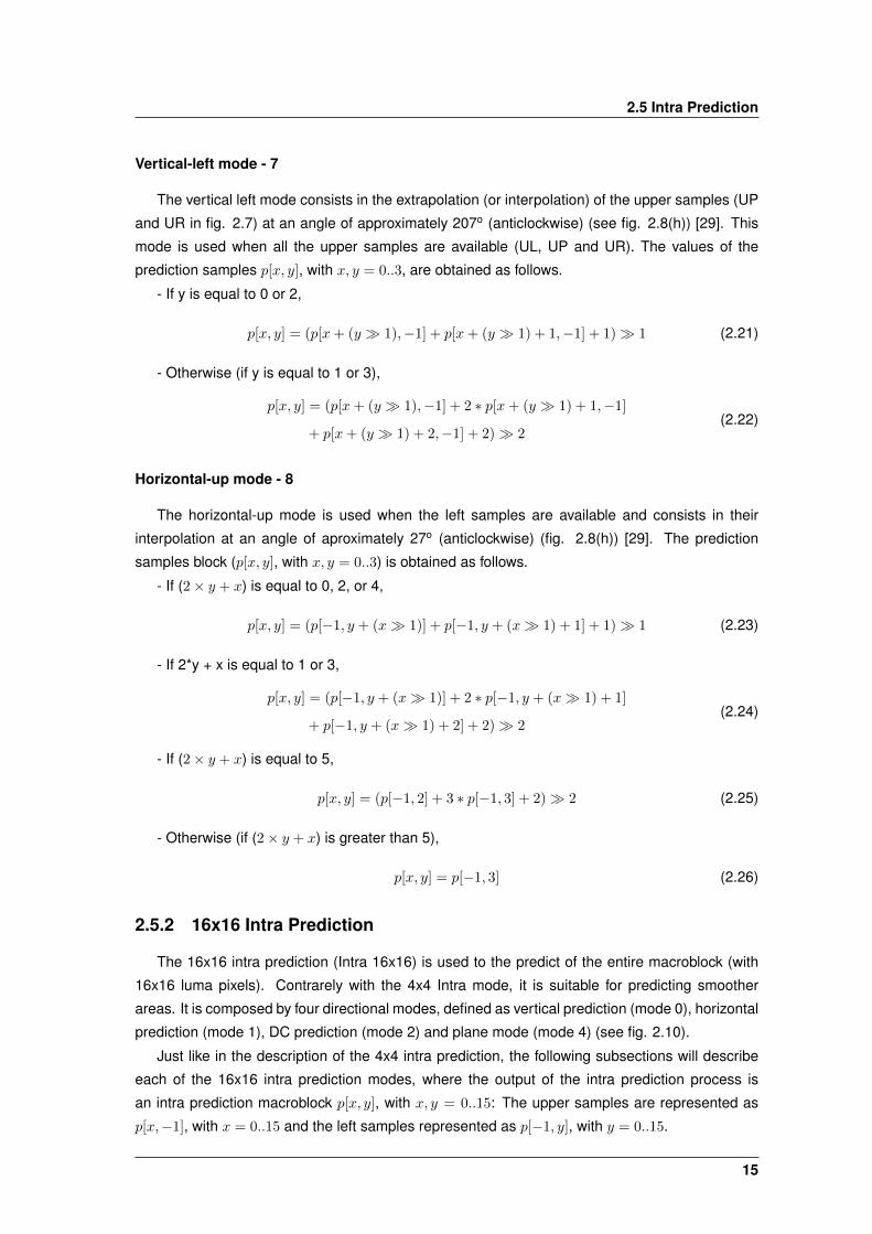
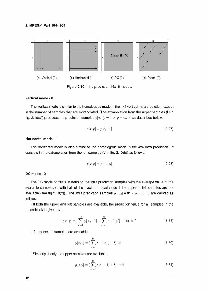
prediction (mode 1), DC prediction (mode 2) and plane mode (mode 4) (see fig. 2.10).
Just like in the description of the 4x4 intra prediction, the following subsections will describe
each of the 16x16 intra prediction modes, where the output of the intra prediction process is
an intra prediction macroblock p[x, y], with x, y = 0..15: The upper samples are represented as
p[x,−1], with x = 0..15 and the left samples represented as p[−1, y], with y = 0..15.
15
2. MPEG-4 Part 10/H.264
(a) Vertical (0). (b) Horizontal (1). (c) DC (2). (d) Plane (3).
Figure 2.10: Intra prediction 16x16 modes.
Vertical mode - 0
The vertical mode is similar to the homologous mode in the 4x4 vertical intra prediction, except
in the number of samples that are extrapolated. The extrapolation from the upper samples (H in
fig. 2.10(a)) produces the prediction samples p[x, y], with x, y = 0..15, as described below:
p[x, y] = p[x,−1] (2.27)
Horizontal mode - 1
The horizontal mode is also similar to the homologous mode in the 4x4 intra prediction. It
consists in the extrapolation from the left samples (V in fig. 2.10(b)) as follows:
p[x, y] = p[−1, y] (2.28)
DC mode - 2
The DC mode consists in defining the intra prediction samples with the average value of the
available samples, or with half of the maximum pixel value if the upper or left samples are un-
available (see fig 2.10(c)). The intra prediction samples p[x, y],with x, y = 0..15 are derived as
follows.
- If both the upper and left samples are available, the prediction value for all samples in the
macroblock is given by:
p[x, y] = (
15∑x′=0
p[x′,−1] +15∑
y′=0
p[−1, y′] + 16)� 5 (2.29)
- If only the left samples are available:
p[x, y] = (
15∑y′=0
p[−1, y′] + 8)� 4 (2.30)
- Similarly, if only the upper samples are available:
p[x, y] = (
15∑x′=0
p[x′,−1] + 8)� 4 (2.31)
16
2.5 Intra Prediction
- Otherwise, if neither the left samples nor the upper ones are available, it is applied the formula
defined in 2.7.
Plane mode - 3
The plane mode applies a linear function to the upper and left samples (H and V in fig 2.10(c))
and is used when both of them are available. It is suitable for areas with a smooth variation of
luminance [29]. The values of the prediction samples p[x, y], with x, y = 0..15, are derived by:
p[x, y] = Clip((a+ b ∗ (x− 7) + c ∗ (y − 7) + 16)� 5) (2.32)
where a, b and c are defined as:
a = 16 ∗ (p[−1, 15] + p[15,−1]) (2.33)
b = (5 ∗H + 32)� 6 (2.34)
c = (5 ∗ V + 32)� 6 (2.35)
and H and V are defined as:
H =
7∑x′=0
(x′ + 1) ∗ (p[8 + x′,−1]− p[6− x′,−1]) (2.36)
V =
7∑y′=0
(y′ + 1) ∗ (p[−1, 8 + y′]− p[−1, 6− y′]) (2.37)
2.5.3 Intra 8x8 Chroma Prediction
Each chrominance component of a macroblock (Cb and Cr) is separately predicted by using
left and upper samples of previously encoded macroblocks. The intra prediction modes of the
chrominances are similar to the 16x16 luminance prediction, except the ordering of the prediction
modes. It also has four prediction modes, denoted to as DC prediction (mode 0), horizontal
prediction (mode 1), vertical prediction (mode 2) and plane prediction (mode 3) [28].
Assuming the obtained prediction samples as p[x, y] (with x, y = 0..8); the left samples as
p[−1, y] (with y = 0..8) and the upper samples as p[x,−1] (with x = 0..8), the intra prediction
process for each mode is defined as follows:
DC mode - 0
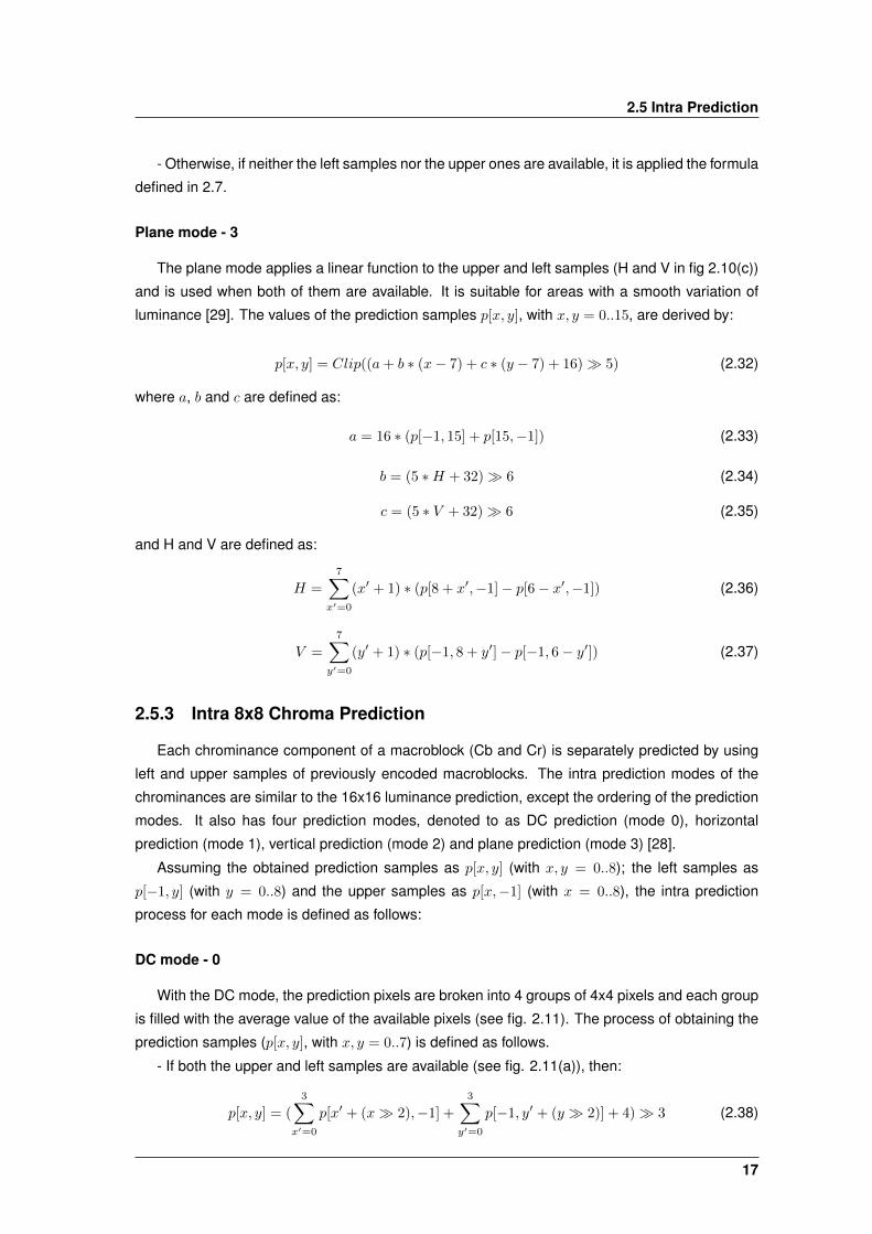
With the DC mode, the prediction pixels are broken into 4 groups of 4x4 pixels and each group
is filled with the average value of the available pixels (see fig. 2.11). The process of obtaining the
prediction samples (p[x, y], with x, y = 0..7) is defined as follows.
- If both the upper and left samples are available (see fig. 2.11(a)), then:
p[x, y] = (
3∑x′=0
p[x′ + (x� 2),−1] +3∑
y′=0
p[−1, y′ + (y � 2)] + 4)� 3 (2.38)
17
2. MPEG-4 Part 10/H.264
(a) All samples available. (b) Only upper samplesavailable.
(c) Only left samples avail-able.
(d) No samples avail-able.
Figure 2.11: DC mode.
- If only the upper samples are available (see fig. 2.11(b)), then:
p[x, y] = (
3∑y′=0
p[−1, y′ + (y � 2)] + 2)� 2 (2.39)
- If only the left samples are available (see fig. 2.11(c)), then:
p[x, y] = (
3∑x′=0
p[x′ + (x� 2),−1] + 2)� 2 (2.40)
- Otherwise, if there are no available samples (see fig. 2.11(d)), then each prediction sample
is filled as defined in equation 2.7.
Horizontal mode - 1
The horizontal mode is used when the left samples are available. Just like the homologous
16x16 luminance mode (see fig. 2.10(b)), it consist in the extrapolation of the left samples. The
values of the prediction pixels p[x, y] (with x, y = 0..7) are derived in equation 2.28.
Vertical mode - 2
The vertical mode is used when the upper samples are available. If has the same behaviour
then the homologous luminance 16x16 mode (fig. 2.10(a)). The values of the prediction pixels
p[x, y] (with x, y = 0..7) are derived in equation 2.27.
18

2.6 Transform Coding
Plane mode - 3
The plane mode in the chrominance prediction is similar to the plane mode in the 16x16
luminance prediction (see fig. 2.10(d)). The values of the prediction pixels (p[x, y], with x, y = 0..7)
are derived by:
p[x, y] = Clip((a+ b ∗ (x− 3) + c ∗ (y − 3) + 16)� 5) (2.41)
where a, b and c are defined as:
a = 16 ∗ (p[−1, 7] + p[7,−1]) (2.42)
b = (17 ∗H + 16)� 5 (2.43)
c = (17 ∗ V + 16)� 5 (2.44)
and H and V are specified as:
H =
4∑x′=1
x′ ∗ (p[3 + x′,−1]− p[3− x′,−1]) (2.45)
V =
4∑y′=1
y′ ∗ (p[−1, 3 + y′]− p[−1, 3− y′]) (2.46)
2.6 Transform Coding
The transform coding module processes the residual signal obtained in the prediction process.
It is formed by two parts: transform and quantization. The transform part allows the mapping of
the image pixels from the spatial domain into the frequency domain, in order to emphasize the
spatial redundancies in the image plane. The process is fully reversible without any loss of data
[28, 30]. The quantization part allows the suppression of irrelevancies, by removing the less
significant data. It is this process the responsible for the lossy compression in the H.264/AVC.
After the quantization process, the quantized transform coefficients are then scanned in a zigzag
order and transmitted using an entropy coding method.
2.6.1 Transform Module
The transform module in the H264/AVC is based on a two-dimensional Discret Cosine Trans-
form (DCT). Unlike the 8x8 DCT that is used by the previous standards, in the H.264/AVC, the
transform is applied mainly in blocks of 4x4 pixels, to reduce the spatial correlation. However, for
performance reasons the H264/AVC uses an integer approximation of the real DCT, in order to
allow its computation by only using 16 bit integer arithmetic operations [17, 26, 30]. The result of
the transform process (Y) applied to a block of data (X) can be obtained through equation 2.47
(where matrix H and its transpose HT are referred to as the transformation kernels).
Y = HXHT (2.47)
19
2. MPEG-4 Part 10/H.264
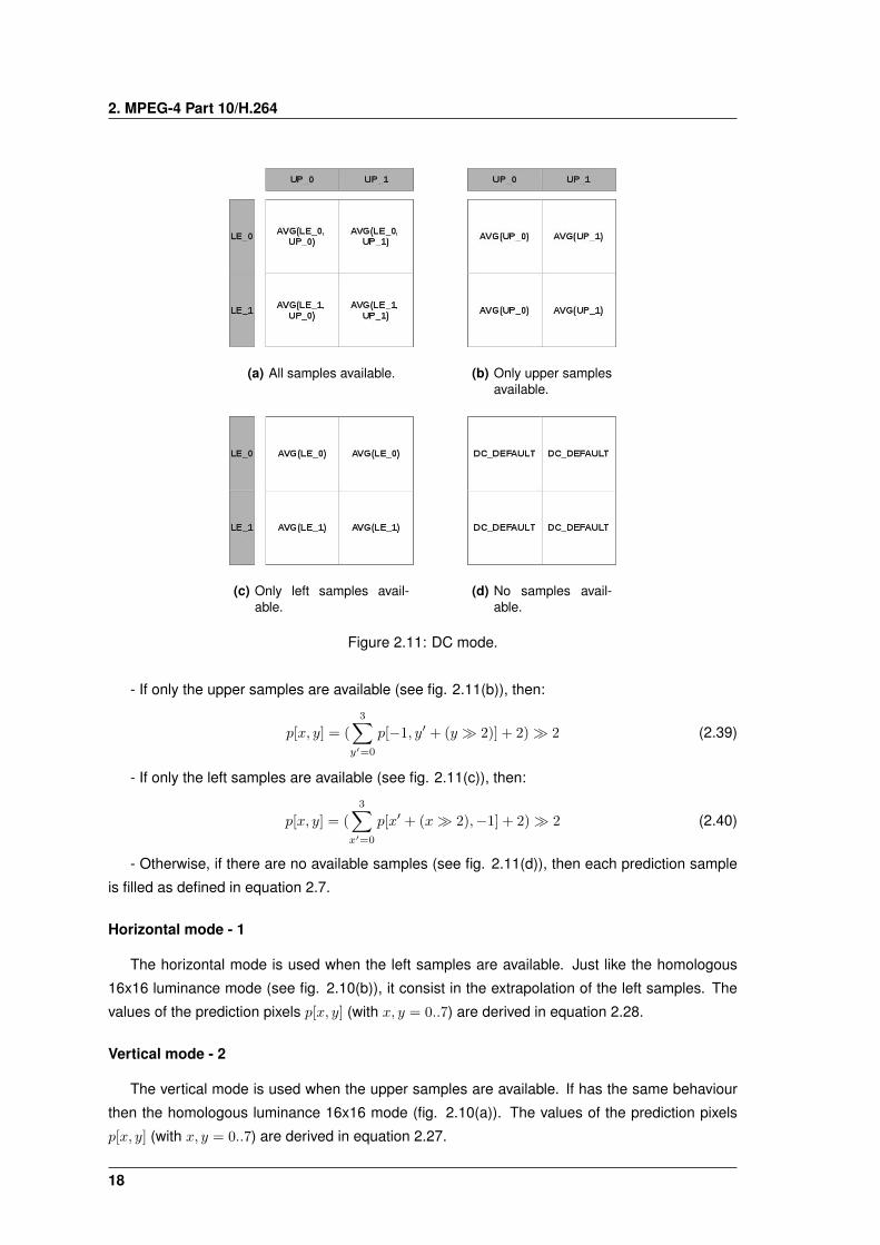
Figure 2.12: Result of a 2D DCT function.
H1 =
1 1 1 12 1 −1 −21 −1 −1 11 −2 2 −1
H2 =
1 1 1 11 1 −1 −11 −1 −1 11 −1 1 −1
H3 =
[1 11 −1
](2.48)
Depending on the adopted prediction mode, three different types of transforms may be used
[26]. The first one (H1 in equation 2.48), with 4x4 coefficients, is applied to all prediction residual
blocks, resulting in one DC and 15 AC coefficients per block (see fig. 2.12)[1].
If a given luminance macroblock is predicted using the 16x16 intra-prediction, the first trans-
form produces sixteen 4x4 coefficients blocks. The DC coefficients of each 4x4 blocks are subse-
quently grouped into a single 4x4 block and are further transformed using the Hadamard Trans-
form (H2 in equation 2.48).
To process the chrominance macroblocks, the first transform (H1) produces four 4x4 coeffi-
cient blocks, whose DC coefficients are subsequently grouped into a single 2x2 block and further
transformed with a Hadamard Transform (H3 in equation 2.48).
2.6.2 Quantization Module
The quantization module controls the amount of signal loss that is introduced, in order to
achieve the desired amount of compression. After being computed, the transform coefficients
are scaled to eliminate the blocks’ less significant values. The H.264 standard has 52 values for
the quantization step. This wide range of step sizes allows the encoder to accurately and flexibly
manipulate the trade-off between bit rate and quality [42].
For a given block (X) and quantization step (Qs), the quantization is performed by equation
2.49, where Xq is the resulting scaled block and f(Qs) controls the quantization width near the
dead-zone 2. The inverse quantization block (Xr) is obtained by the equation 2.50 [17].
Xq(i, j) = sign{X(i, j)} |X(i, j)|+ f(Qs)
Qs(2.49)
Xr(i, j) = QsXq(i, j) (2.50)
2The values near the DC value are enlarged; beyond these zone the step size tends to be uniform.
20
2.7 Profiles and Levels
2.7 Profiles and Levels
In order to address the different requirements that are imposed by several applications, such as
error resilience, compression efficiency, latency or complexity, the H.264/AVC standard specifies
a set of profiles that give support to the definition of of the entire syntax options defined by the
standard. Among others, the three main profiles are defined and denoted by Baseline Profile,
Main Profile and Extended Profile [3, 26, 41]. The Baseline Profile is the simplest profile and
is targeted for applications with low complexity and low latency requirements. The Main Profile
offers the best quality at the cost of higher complexity and the Extended Profile is considered to
be a superset of the Baseline Profile. For each profile, the standard also defines fifteen levels that
specify the upper bounds for the bitstream or the lower bounds for the decoder capabilities. More
detailed information about H.264/AVC profiles and levels can be found in [39] and [26].
21

2. MPEG-4 Part 10/H.264
22
3Nvidia’s GPU Parallel Programming
Platform
Contents3.1 CUDA Programming Model . . . . . . . . . . . . . . . . . . . . . . . . . . . . . . 243.2 Fermi GPU’s Architecture . . . . . . . . . . . . . . . . . . . . . . . . . . . . . . 31
23
3. Nvidia’s GPU Parallel Programming Platform
The evolution of single-core CPUs according to Moore’s law has slowed-down since 2003, due
to energy consumption and heat-dissipation issues [13]. Consequently, the processing power evo-
lution of CPUs has gradually changed to a multicore model, where multiple CPUs are simultane-
ously used and the number of offered cores is being doubled with each semiconductor processing
generation. Nowadays, with the existence of multicore CPUs and many-core GPUs, many main-
stream processor chips are now parallel systems and their parallelism continues to scale with
Moore’s law [24].
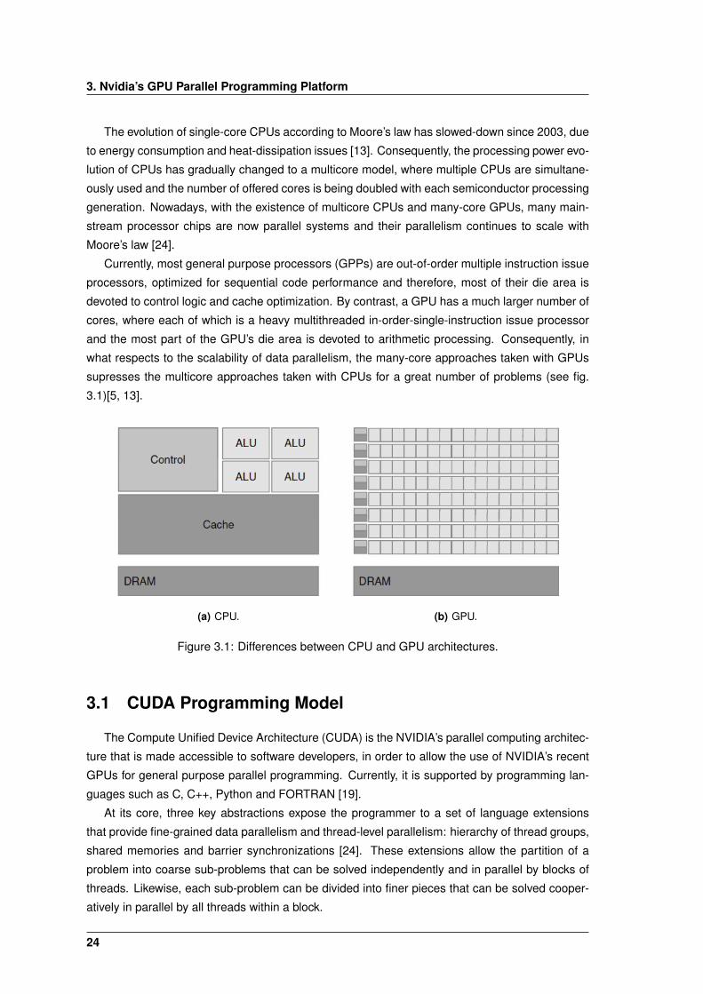
Currently, most general purpose processors (GPPs) are out-of-order multiple instruction issue
processors, optimized for sequential code performance and therefore, most of their die area is
devoted to control logic and cache optimization. By contrast, a GPU has a much larger number of
cores, where each of which is a heavy multithreaded in-order-single-instruction issue processor
and the most part of the GPU’s die area is devoted to arithmetic processing. Consequently, in
what respects to the scalability of data parallelism, the many-core approaches taken with GPUs
supresses the multicore approaches taken with CPUs for a great number of problems (see fig.
3.1)[5, 13].
(a) CPU. (b) GPU.
Figure 3.1: Differences between CPU and GPU architectures.
3.1 CUDA Programming Model
The Compute Unified Device Architecture (CUDA) is the NVIDIA’s parallel computing architec-
ture that is made accessible to software developers, in order to allow the use of NVIDIA’s recent
GPUs for general purpose parallel programming. Currently, it is supported by programming lan-
guages such as C, C++, Python and FORTRAN [19].
At its core, three key abstractions expose the programmer to a set of language extensions
that provide fine-grained data parallelism and thread-level parallelism: hierarchy of thread groups,
shared memories and barrier synchronizations [24]. These extensions allow the partition of a
problem into coarse sub-problems that can be solved independently and in parallel by blocks of
threads. Likewise, each sub-problem can be divided into finer pieces that can be solved cooper-
atively in parallel by all threads within a block.
24
3.1 CUDA Programming Model
Each CUDA program comprises both the host and the device code1 and consists of one or
more execution parts that are issued to the CPU or to the GPU. The parts of code with a higher
data-level parallelism are usually executed in the GPU, leaving the remaining parts to be imple-
mented in the CPU.
Besides the support for different languages, CUDA can be used from different APIs, such as
the low-level driver API, the runtime API or high-level APIs. The high-level APIs allow a quicker
code development that is easy to maintain, but the development is isolated from the hardware and
only a subset of the hardware capabilities may be exposed. On the other hand, the CUDA runtime
API gives access to all the programmable features of the GPU, with some syntax additions to the
developed code. The low-level API allows a higher control of the hardware features, at the cost of
increased code size and more focus on the details of the API interface rather than on the actual
work of the task.
Modern versions of CUDA allow the developers to use all the three levels of APIs. Thus, a
piece of code can be initially written with a high-level API and then refactored in order to use
some special characteristics of the low-level API [6].
3.1.1 CUDA Runtime
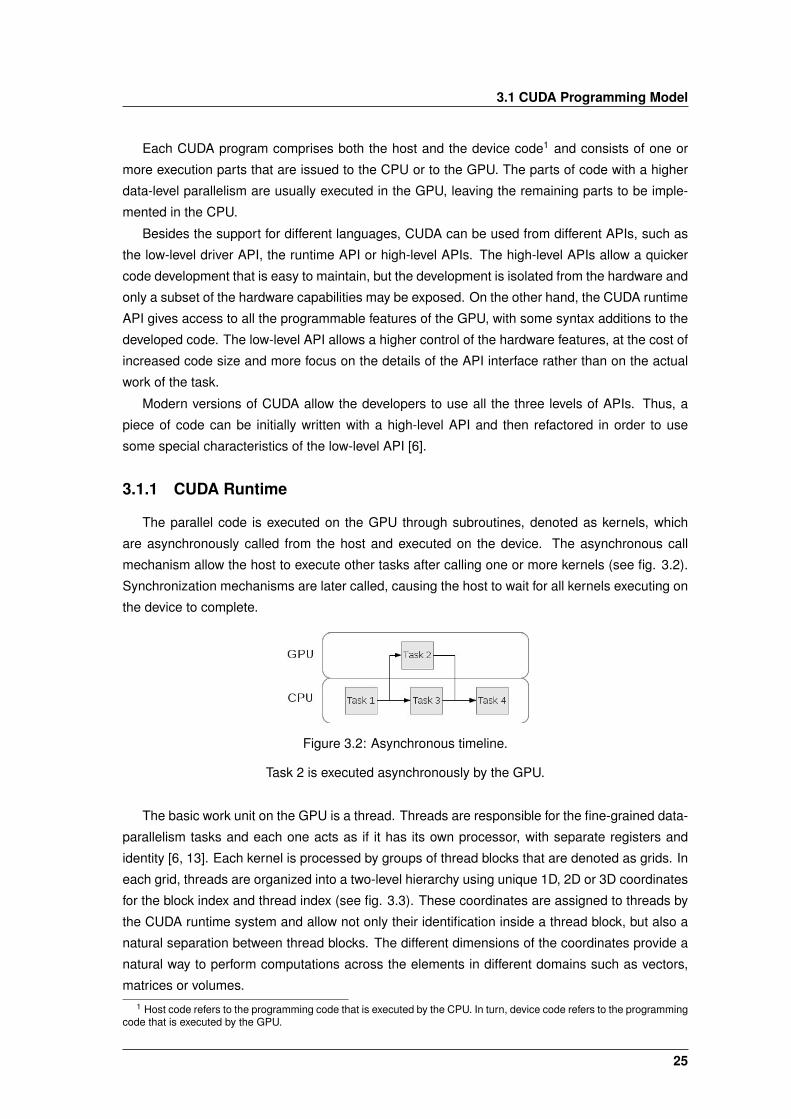
The parallel code is executed on the GPU through subroutines, denoted as kernels, which
are asynchronously called from the host and executed on the device. The asynchronous call
mechanism allow the host to execute other tasks after calling one or more kernels (see fig. 3.2).
Synchronization mechanisms are later called, causing the host to wait for all kernels executing on
the device to complete.
Figure 3.2: Asynchronous timeline.
Task 2 is executed asynchronously by the GPU.
The basic work unit on the GPU is a thread. Threads are responsible for the fine-grained data-
parallelism tasks and each one acts as if it has its own processor, with separate registers and
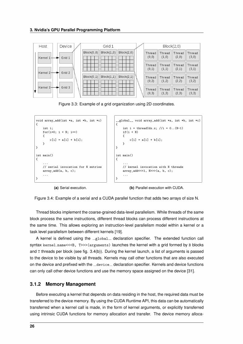
identity [6, 13]. Each kernel is processed by groups of thread blocks that are denoted as grids. In
each grid, threads are organized into a two-level hierarchy using unique 1D, 2D or 3D coordinates
for the block index and thread index (see fig. 3.3). These coordinates are assigned to threads by
the CUDA runtime system and allow not only their identification inside a thread block, but also a
natural separation between thread blocks. The different dimensions of the coordinates provide a
natural way to perform computations across the elements in different domains such as vectors,
matrices or volumes.1 Host code refers to the programming code that is executed by the CPU. In turn, device code refers to the programming
code that is executed by the GPU.
25
3. Nvidia’s GPU Parallel Programming Platform
Figure 3.3: Example of a grid organization using 2D coordinates.
void array_add(int *a, int *b, int *c)
{
int i;
for(i=0; i < N; i++)
{
c[i] = a[i] + b[i];
}
}
int main()
{
...
// serial invocation for N entries
array_add(a, b, c);
...
}
(a) Serial execution.
__global__ void array_add(int *a, int *b, int *c)
{
int i = threadIdx.x; //i = 0..(N-1)
if(i < N)
{
c[i] = a[i] + b[i];
}
}
int main()
{
...
// kernel invocation with N threads
array_add<<<1, N>>>(a, b, c);
...
}
(b) Parallel execution with CUDA.
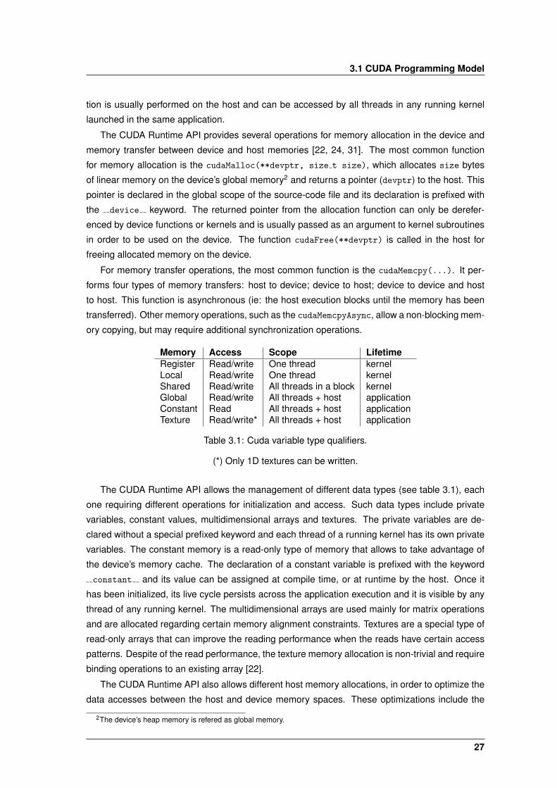
Figure 3.4: Example of a serial and a CUDA parallel function that adds two arrays of size N.
Thread blocks implement the coarse-grained data-level parallelism. While threads of the same
block process the same instructions, different thread blocks can process different instructions at
the same time. This allows exploring an instruction-level parallelism model within a kernel or a
task level parallelism between different kernels [19].
A kernel is defined using the global declaration specifier. The extended function call
syntax kernel name<<<B, T>>>(arguments) launches the kernel with a grid formed by B blocks
and T threads per block (see fig. 3.4(b)). During the kernel launch, a list of arguments is passed
to the device to be visible by all threads. Kernels may call other functions that are also executed
on the device and prefixed with the device declaration specifier. Kernels and device functions
can only call other device functions and use the memory space assigned on the device [31].
3.1.2 Memory Management
Before executing a kernel that depends on data residing in the host, the required data must be
transferred to the device memory. By using the CUDA Runtime API, this data can be automatically
transferred when a kernel call is made, in the form of kernel arguments, or explicitly transferred
using intrinsic CUDA functions for memory allocation and transfer. The device memory alloca-
26
3.1 CUDA Programming Model
tion is usually performed on the host and can be accessed by all threads in any running kernel
launched in the same application.
The CUDA Runtime API provides several operations for memory allocation in the device and
memory transfer between device and host memories [22, 24, 31]. The most common function
for memory allocation is the cudaMalloc(**devptr, size t size), which allocates size bytes
of linear memory on the device’s global memory2 and returns a pointer (devptr) to the host. This
pointer is declared in the global scope of the source-code file and its declaration is prefixed with
the device keyword. The returned pointer from the allocation function can only be derefer-
enced by device functions or kernels and is usually passed as an argument to kernel subroutines
in order to be used on the device. The function cudaFree(**devptr) is called in the host for
freeing allocated memory on the device.
For memory transfer operations, the most common function is the cudaMemcpy(...). It per-
forms four types of memory transfers: host to device; device to host; device to device and host
to host. This function is asynchronous (ie: the host execution blocks until the memory has been
transferred). Other memory operations, such as the cudaMemcpyAsync, allow a non-blocking mem-
ory copying, but may require additional synchronization operations.
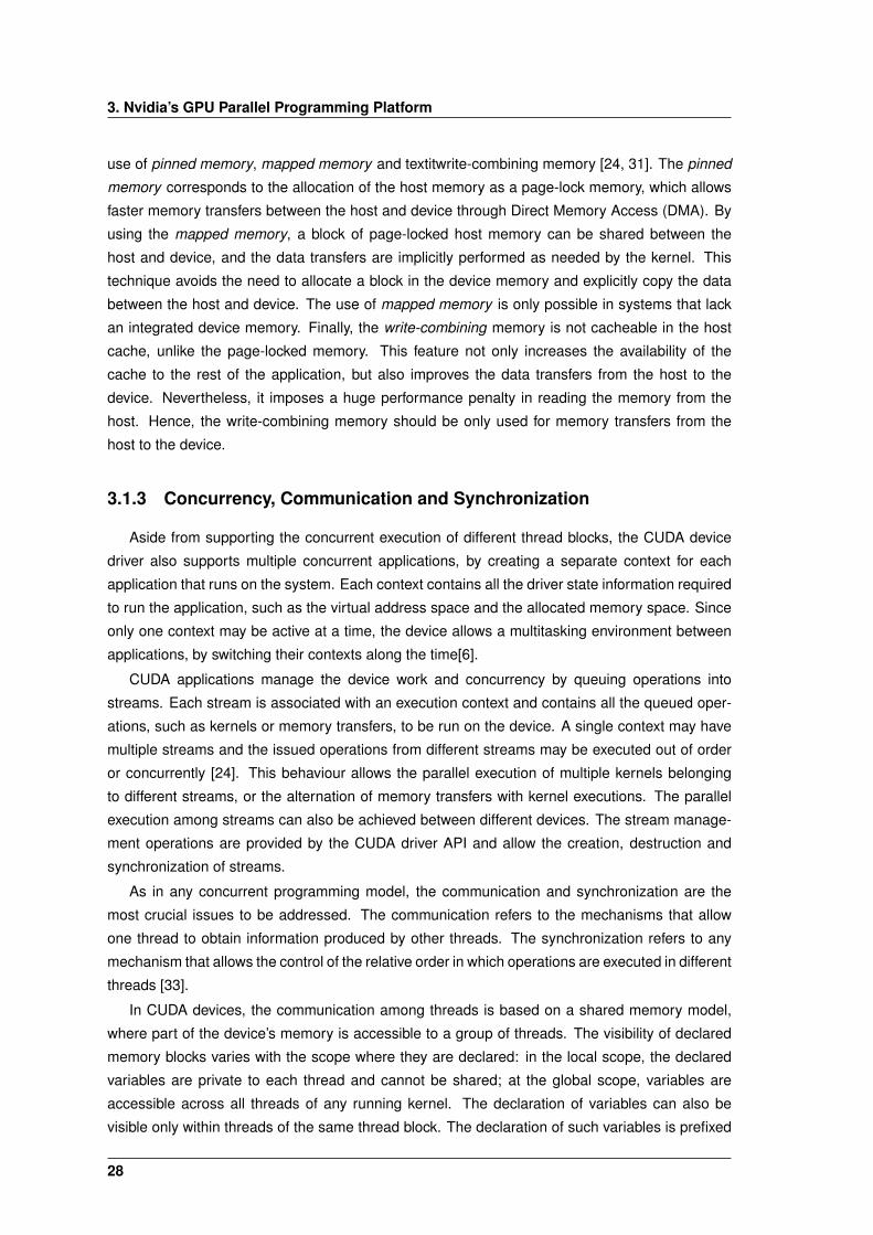
Memory Access Scope LifetimeRegister Read/write One thread kernelLocal Read/write One thread kernelShared Read/write All threads in a block kernelGlobal Read/write All threads + host applicationConstant Read All threads + host applicationTexture Read/write* All threads + host application
Table 3.1: Cuda variable type qualifiers.
(*) Only 1D textures can be written.
The CUDA Runtime API allows the management of different data types (see table 3.1), each
one requiring different operations for initialization and access. Such data types include private
variables, constant values, multidimensional arrays and textures. The private variables are de-
clared without a special prefixed keyword and each thread of a running kernel has its own private
variables. The constant memory is a read-only type of memory that allows to take advantage of
the device’s memory cache. The declaration of a constant variable is prefixed with the keyword
constant and its value can be assigned at compile time, or at runtime by the host. Once it
has been initialized, its live cycle persists across the application execution and it is visible by any
thread of any running kernel. The multidimensional arrays are used mainly for matrix operations
and are allocated regarding certain memory alignment constraints. Textures are a special type of
read-only arrays that can improve the reading performance when the reads have certain access
patterns. Despite of the read performance, the texture memory allocation is non-trivial and require
binding operations to an existing array [22].
The CUDA Runtime API also allows different host memory allocations, in order to optimize the
data accesses between the host and device memory spaces. These optimizations include the
2The device’s heap memory is refered as global memory.
27
3. Nvidia’s GPU Parallel Programming Platform
use of pinned memory, mapped memory and textitwrite-combining memory [24, 31]. The pinned
memory corresponds to the allocation of the host memory as a page-lock memory, which allows
faster memory transfers between the host and device through Direct Memory Access (DMA). By
using the mapped memory, a block of page-locked host memory can be shared between the
host and device, and the data transfers are implicitly performed as needed by the kernel. This
technique avoids the need to allocate a block in the device memory and explicitly copy the data
between the host and device. The use of mapped memory is only possible in systems that lack
an integrated device memory. Finally, the write-combining memory is not cacheable in the host
cache, unlike the page-locked memory. This feature not only increases the availability of the
cache to the rest of the application, but also improves the data transfers from the host to the
device. Nevertheless, it imposes a huge performance penalty in reading the memory from the
host. Hence, the write-combining memory should be only used for memory transfers from the
host to the device.
3.1.3 Concurrency, Communication and Synchronization
Aside from supporting the concurrent execution of different thread blocks, the CUDA device
driver also supports multiple concurrent applications, by creating a separate context for each
application that runs on the system. Each context contains all the driver state information required
to run the application, such as the virtual address space and the allocated memory space. Since
only one context may be active at a time, the device allows a multitasking environment between
applications, by switching their contexts along the time[6].
CUDA applications manage the device work and concurrency by queuing operations into
streams. Each stream is associated with an execution context and contains all the queued oper-
ations, such as kernels or memory transfers, to be run on the device. A single context may have
multiple streams and the issued operations from different streams may be executed out of order
or concurrently [24]. This behaviour allows the parallel execution of multiple kernels belonging
to different streams, or the alternation of memory transfers with kernel executions. The parallel
execution among streams can also be achieved between different devices. The stream manage-
ment operations are provided by the CUDA driver API and allow the creation, destruction and
synchronization of streams.
As in any concurrent programming model, the communication and synchronization are the
most crucial issues to be addressed. The communication refers to the mechanisms that allow
one thread to obtain information produced by other threads. The synchronization refers to any
mechanism that allows the control of the relative order in which operations are executed in different
threads [33].
In CUDA devices, the communication among threads is based on a shared memory model,
where part of the device’s memory is accessible to a group of threads. The visibility of declared
memory blocks varies with the scope where they are declared: in the local scope, the declared
variables are private to each thread and cannot be shared; at the global scope, variables are
accessible across all threads of any running kernel. The declaration of variables can also be
visible only within threads of the same thread block. The declaration of such variables is prefixed
28

3.1 CUDA Programming Model
with the keyword shared and they persist during the lifetime of the kernel where they are
declared.
The synchronization has the purpose of implementing the atomicity in certain operations, or
to delay them until some necessary precondition holds [33]. The CUDA API has intrinsic func-
tions to perform read-modify-write atomic operations on shared or global memory positions and
to synchronize thread execution to coordinate memory accesses [24, 31]. The synchronization
functions act on the thread level or on the stream level. The function syncthreads() acts as a
barrier at which all threads in a thread block must wait before any is allowed to proceed3. On the
stream level, the function cudaStreamSynchronize(cudaStream t stream) blocks the execution
on the host until stream has completed all operations. Because these functions that are used for
synchronizing threads are called inside the device, they have a lower latency than the functions
used to synchronize streams, which are called by the device driver.
3.1.4 Compute Capabilities
CUDA devices are categorized by compute capabilities, which define their available features
and restrictions, such as the support for atomic operations, or the maximum number of concurrent
threads. The compute capability follows an incremental version system ,formed by a major and
minor revision numbers (see table 3.2). The higher compute capability versions are supersets of
lower ones. Hence, the devices with a higher compute capability support all the previous compute
capability features [6, 21, 31].
Compute Capability Featurescompute 1.0 Basic featurescompute 1.1 +atomic memory operations on global memory
compute 1.2 +atomic memory operations on shared memory+vote instructions
compute 1.3 +double precision floating point supportcompute 2.0 +Fermi support
Table 3.2: Compute capability features list.
CUDA applications are compiled with the support of a given compute capability version, no
only to allow the set of optimizations available on that version, but also to limit the minimum
capability version required to run the application. By using higher capability versions, it is allowed
the support of more features and optimizations, but the range of devices where it can be used is
more limited.
3.1.5 Compilation Process
The CUDA source files are suffixed with the extension .cu and contain a mix of host and device
programming code. Then, the NVIDIA compiler (nvcc) separates the host from the device code
during the initial compilation process (see fig. 3.5). The device code can be compiled using an
offline compilation process, and/or mapped into a intermediary assembly-like language, by using
3The CUDA API does not provide functions to synchronize threads in different blocks.
29
3. Nvidia’s GPU Parallel Programming Platform
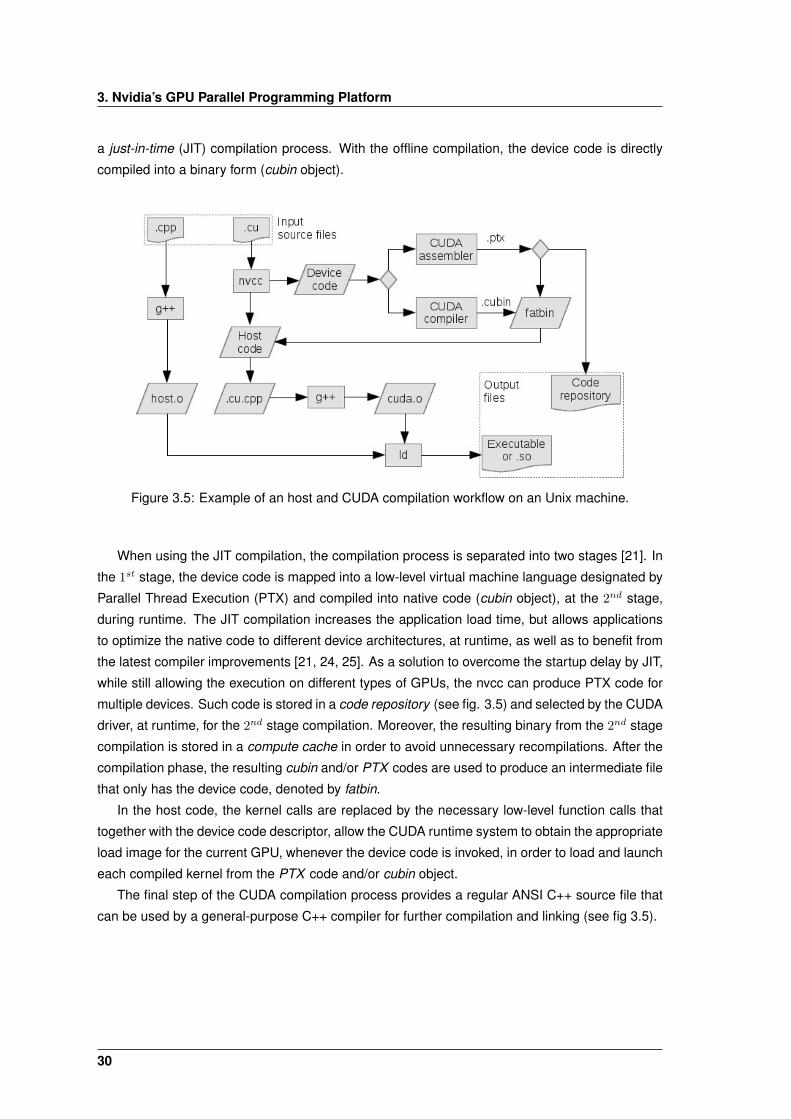
a just-in-time (JIT) compilation process. With the offline compilation, the device code is directly
compiled into a binary form (cubin object).
Figure 3.5: Example of an host and CUDA compilation workflow on an Unix machine.
When using the JIT compilation, the compilation process is separated into two stages [21]. In
the 1st stage, the device code is mapped into a low-level virtual machine language designated by
Parallel Thread Execution (PTX) and compiled into native code (cubin object), at the 2nd stage,
during runtime. The JIT compilation increases the application load time, but allows applications
to optimize the native code to different device architectures, at runtime, as well as to benefit from
the latest compiler improvements [21, 24, 25]. As a solution to overcome the startup delay by JIT,
while still allowing the execution on different types of GPUs, the nvcc can produce PTX code for
multiple devices. Such code is stored in a code repository (see fig. 3.5) and selected by the CUDA
driver, at runtime, for the 2nd stage compilation. Moreover, the resulting binary from the 2nd stage
compilation is stored in a compute cache in order to avoid unnecessary recompilations. After the
compilation phase, the resulting cubin and/or PTX codes are used to produce an intermediate file
that only has the device code, denoted by fatbin.
In the host code, the kernel calls are replaced by the necessary low-level function calls that
together with the device code descriptor, allow the CUDA runtime system to obtain the appropriate
load image for the current GPU, whenever the device code is invoked, in order to load and launch
each compiled kernel from the PTX code and/or cubin object.
The final step of the CUDA compilation process provides a regular ANSI C++ source file that
can be used by a general-purpose C++ compiler for further compilation and linking (see fig 3.5).
30
3.2 Fermi GPU’s Architecture
3.2 Fermi GPU’s Architecture
From the point of view of a CUDA programmer, the knowledge of the underlying GPU archi-
tecture is crucial to solve several issues regarding the performance of a CUDA application. In the
same extent, the awareness of the CUDA runtime limitations allows more efficient approaches to
be taken when implementing a solution to a given problem, such as choosing alternate execution
paths to avoid or compensate for possible bottlenecks.
The newest NVIDIA’s GPU architecture is organized into an array of Streaming-Processors
(SPs)4, denoted by Streaming-Multiprocessors (SMs). Each streaming multiprocessor is capable
of processing simultaneously a massive number of threads and is usually formed by a group of
streaming processors that share the instruction cache and control logic.
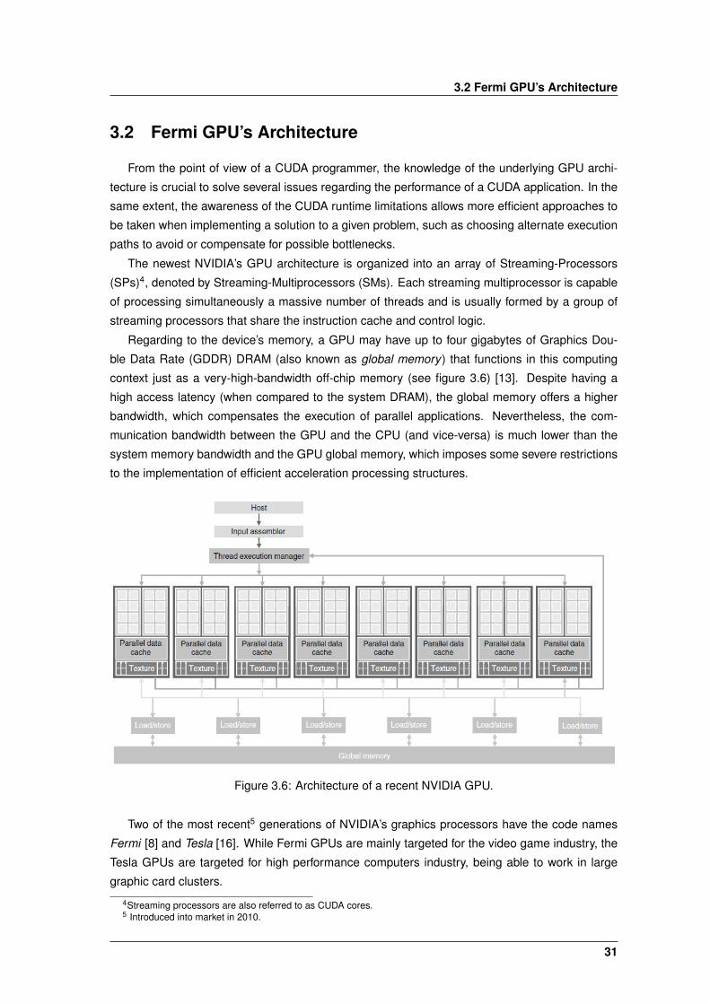
Regarding to the device’s memory, a GPU may have up to four gigabytes of Graphics Dou-
ble Data Rate (GDDR) DRAM (also known as global memory ) that functions in this computing
context just as a very-high-bandwidth off-chip memory (see figure 3.6) [13]. Despite having a
high access latency (when compared to the system DRAM), the global memory offers a higher
bandwidth, which compensates the execution of parallel applications. Nevertheless, the com-
munication bandwidth between the GPU and the CPU (and vice-versa) is much lower than the
system memory bandwidth and the GPU global memory, which imposes some severe restrictions
to the implementation of efficient acceleration processing structures.
Figure 3.6: Architecture of a recent NVIDIA GPU.
Two of the most recent5 generations of NVIDIA’s graphics processors have the code names
Fermi [8] and Tesla [16]. While Fermi GPUs are mainly targeted for the video game industry, the
Tesla GPUs are targeted for high performance computers industry, being able to work in large
graphic card clusters.
4Streaming processors are also referred to as CUDA cores.5 Introduced into market in 2010.
31
3. Nvidia’s GPU Parallel Programming Platform
Since the solution that will be proposed in the scope of this thesis will adopt a Fermi graphics
card, the architecture description that follows will give a greater emphasis to this type of GPU.
When compared to its predecessors, the Fermi GPU architecture brought many enhance-
ments:
• Improved double precision performance;
• Error Check and Correction (ECC) support for graphics memory;
• A true cache memory hierarchy (similar to the x86), thus allowing parallel algorithms to use
the GPU’s shared memory;
• Increased shared memory to 64 Kbytes;
• A faster context switching between application programs;
• Faster atomic operations, to allow parallel algorithms to use faster read-modify- write atomic
operations.
3.2.1 Streaming Multiprocessor
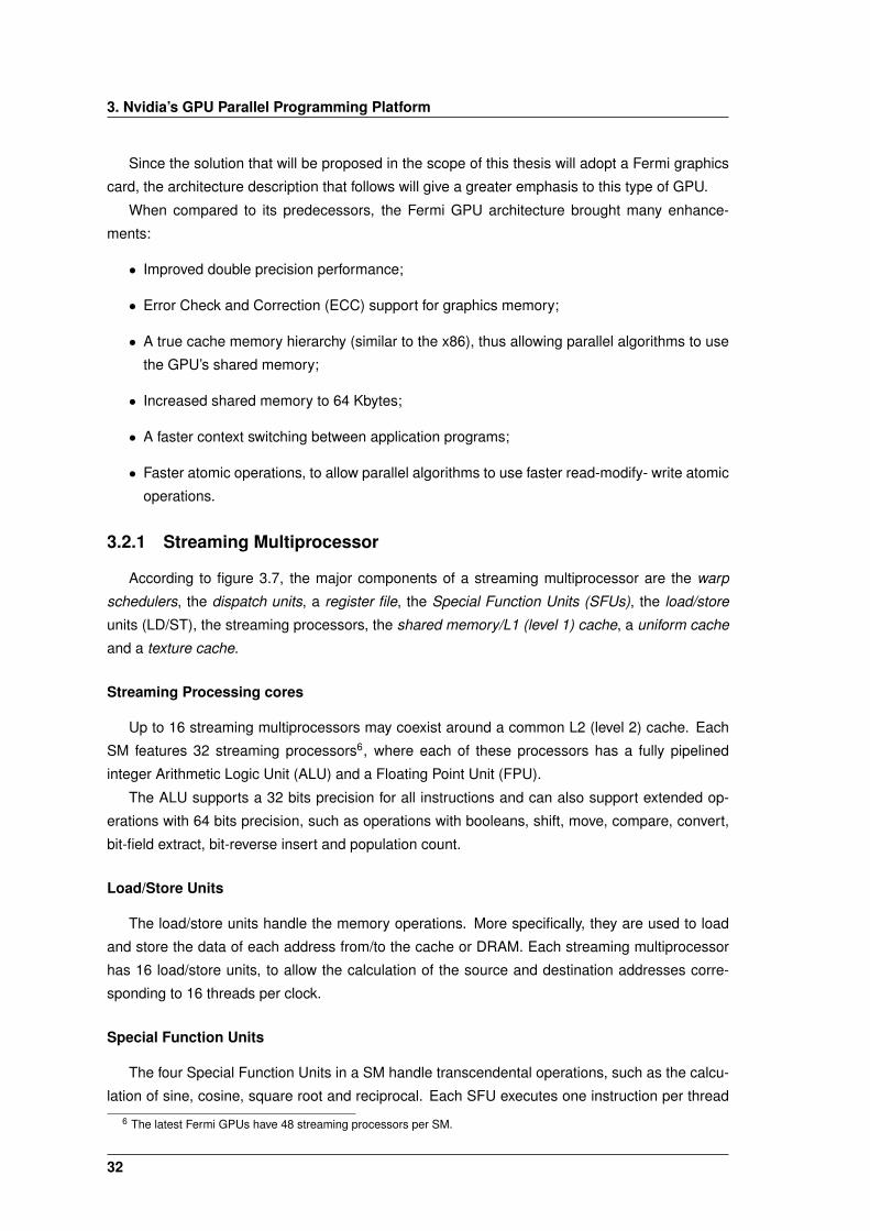
According to figure 3.7, the major components of a streaming multiprocessor are the warp
schedulers, the dispatch units, a register file, the Special Function Units (SFUs), the load/store
units (LD/ST), the streaming processors, the shared memory/L1 (level 1) cache, a uniform cache
and a texture cache.
Streaming Processing cores
Up to 16 streaming multiprocessors may coexist around a common L2 (level 2) cache. Each
SM features 32 streaming processors6, where each of these processors has a fully pipelined
integer Arithmetic Logic Unit (ALU) and a Floating Point Unit (FPU).
The ALU supports a 32 bits precision for all instructions and can also support extended op-
erations with 64 bits precision, such as operations with booleans, shift, move, compare, convert,
bit-field extract, bit-reverse insert and population count.
Load/Store Units
The load/store units handle the memory operations. More specifically, they are used to load
and store the data of each address from/to the cache or DRAM. Each streaming multiprocessor
has 16 load/store units, to allow the calculation of the source and destination addresses corre-
sponding to 16 threads per clock.
Special Function Units
The four Special Function Units in a SM handle transcendental operations, such as the calcu-
lation of sine, cosine, square root and reciprocal. Each SFU executes one instruction per thread
6 The latest Fermi GPUs have 48 streaming processors per SM.
32
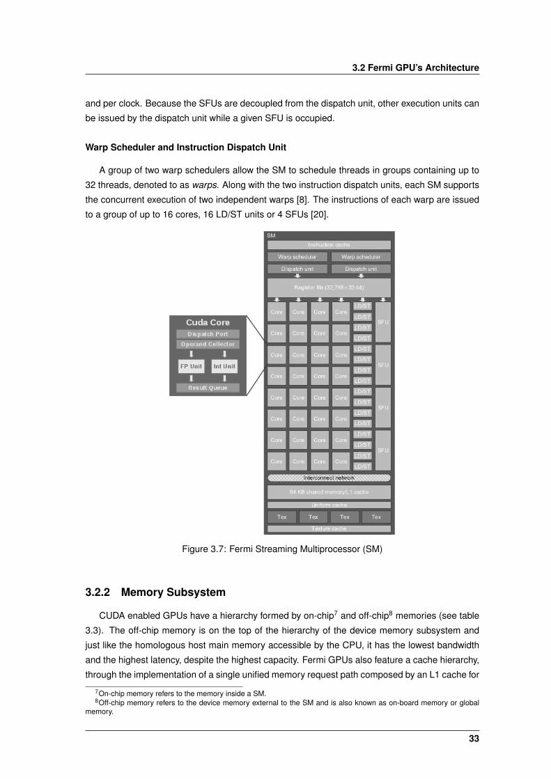
3.2 Fermi GPU’s Architecture
and per clock. Because the SFUs are decoupled from the dispatch unit, other execution units can
be issued by the dispatch unit while a given SFU is occupied.
Warp Scheduler and Instruction Dispatch Unit
A group of two warp schedulers allow the SM to schedule threads in groups containing up to
32 threads, denoted to as warps. Along with the two instruction dispatch units, each SM supports
the concurrent execution of two independent warps [8]. The instructions of each warp are issued
to a group of up to 16 cores, 16 LD/ST units or 4 SFUs [20].
Figure 3.7: Fermi Streaming Multiprocessor (SM)
3.2.2 Memory Subsystem
CUDA enabled GPUs have a hierarchy formed by on-chip7 and off-chip8 memories (see table
3.3). The off-chip memory is on the top of the hierarchy of the device memory subsystem and
just like the homologous host main memory accessible by the CPU, it has the lowest bandwidth
and the highest latency, despite the highest capacity. Fermi GPUs also feature a cache hierarchy,
through the implementation of a single unified memory request path composed by an L1 cache for
7On-chip memory refers to the memory inside a SM.8Off-chip memory refers to the device memory external to the SM and is also known as on-board memory or global
memory.
33
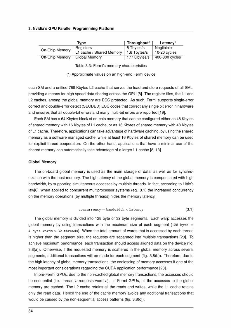
3. Nvidia’s GPU Parallel Programming Platform
Type Throughput* Latency*
On-Chip Memory Registers 8 Tbytes/s NeglibibleL1 cache / Shared Memory 1,6 Tbytes/s 10-20 cycles
Off-Chip Memory Global Memory 177 Gbytes/s 400-800 cycles
Table 3.3: Fermi’s memory characteristics
(*) Approximate values on an high-end Fermi device
each SM and a unified 768 Kbytes L2 cache that serves the load and store requests of all SMs,
providing a means for high speed data sharing across the GPU [8]. The register files, the L1 and
L2 caches, among the global memory are ECC protected. As such, Fermi supports single-error
correct and double-error detect (SECDED) ECC codes that correct any single bit error in hardware
and ensures that all double-bit errors and many multi-bit errors are reported [19].
Each SM has a 64 Kbytes block of on-chip memory that can be configured either as 48 Kbytes
of shared memory with 16 Kbytes of L1 cache, or as 16 Kbytes of shared memory with 48 Kbytes
of L1 cache. Therefore, applications can take advantage of hardware caching, by using the shared
memory as a software managed cache, while at least 16 Kbytes of shared memory can be used
for explicit thread cooperation. On the other hand, applications that have a minimal use of the
shared memory can automatically take advantage of a larger L1 cache [8, 13].
Global Memory
The on-board global memory is used as the main storage of data, as well as for synchro-
nization with the host memory. The high latency of the global memory is compensated with high
bandwidth, by supporting simultaneous accesses by multiple threads. In fact, according to Little’s
law[6], when applied to concurrent multiprocessor systems (eq. 3.1) the increased concurrency
on the memory operations (by multiple threads) hides the memory latency.
concurrency = bandwidth× latency (3.1)
The global memory is divided into 128 byte or 32 byte segments. Each warp accesses the
global memory by using transactions with the maximum size of each segment (128 byte =
4 byte words × 32 threads). When the total amount of words that is accessed by each thread
is higher than the segment size, the requests are separated into multiple transactions [23]. To
achieve maximum performance, each transaction should access aligned data on the device (fig.
3.8(a)). Otherwise, if the requested memory is scattered in the global memory across several
segments, additional transactions will be made for each segment (fig. 3.8(b)). Therefore, due to
the high latency of global memory transactions, the coalescing of memory accesses if one of the
most important considerations regarding the CUDA application performance [23].
In pre-Fermi GPUs, due to the non-cached global memory transactions, the accesses should
be sequential (i.e. thread n requests word n). In Fermi GPUs, all the accesses to the global
memory are cached. The L2 cache retains all the reads and writes, while the L1 cache retains
only the read data. Hence the use of the cache memory avoids any additional transactions that
would be caused by the non-sequential access patterns (fig. 3.8(c)).
34

3.2 Fermi GPU’s Architecture
(a) Coalesced access. (b) Misaligned access. (c) Out of sequence access.
Figure 3.8: Global memory coalescing.
Registers
Each SM has a 128 kilobyte register file (32K registers of 32-bit) to hold frequently used pro-
grammer and compiler generated variables, in order to reduce the access latency and to conserve
memory bandwidth [20]. Furthermore, it also allows the on-chip execution and performance im-
provement on multiple threads. The number of register per thread varies not only with the re-
sources required by each thread (local variables), but also with the number of threads per thread
block. Hence, the maximum number of register per thread varies from 21 registers, if the SM is
running with 1536 threads, to a maximum of 63 registers. [6].
Local Memory
The local memory is used to accommodate private variables of each thread. A private variable
may be located either in the registers or in the device memory. Generally, private variables reside
in the registers, except the large structures of arrays that would consume excessive register space
or any variable that is spilled by the compiler to the device memory when the kernel is using more
registers than the available on the SM. Aside from the visibility between threads, there is no
significant difference between the local and global memories. Both of them refer to the same
off-chip physical memory location. Hence, the access to the local memory is as expensive as the
access to the global memory [23].
L1 and L2 Cache Memory
The cache memory is used to exploit the temporal and spatial locality of data, in order to
minimize the global memory transactions and keep data in a faster memory. The temporal locality
is exploited whenever it is assumed that a recently used variable is likely to be reused in a near
future (Least Recently Used (LRU) behaviour). The exploitation of the spatial locality consists in
caching the neighbouring data, assuming that the adjacent memory locations are likely to be used
in a near future. It is highly useful for rendering applications that mainly use 2D data types. By
default, all the accesses to the global memory are cached. Hence, the local variables residing
in the device memory and in the spilled registers can be cached, which can compensate for the
excessive usage of registers per thread, but may increase the cache miss rate [6].
The unified 768 Kbytes L2 cache stores data in a LRU fashion, in order to avoid the global
memory bandwidth bottlenecks, such as the high latency and the irregular memory access pat-
terns, that otherwise would exhibit extremely poor performance. The unified model of the L2
cache guarantees a coherence view to all SMs, and avoids the invalidation and flushed mecha-
35
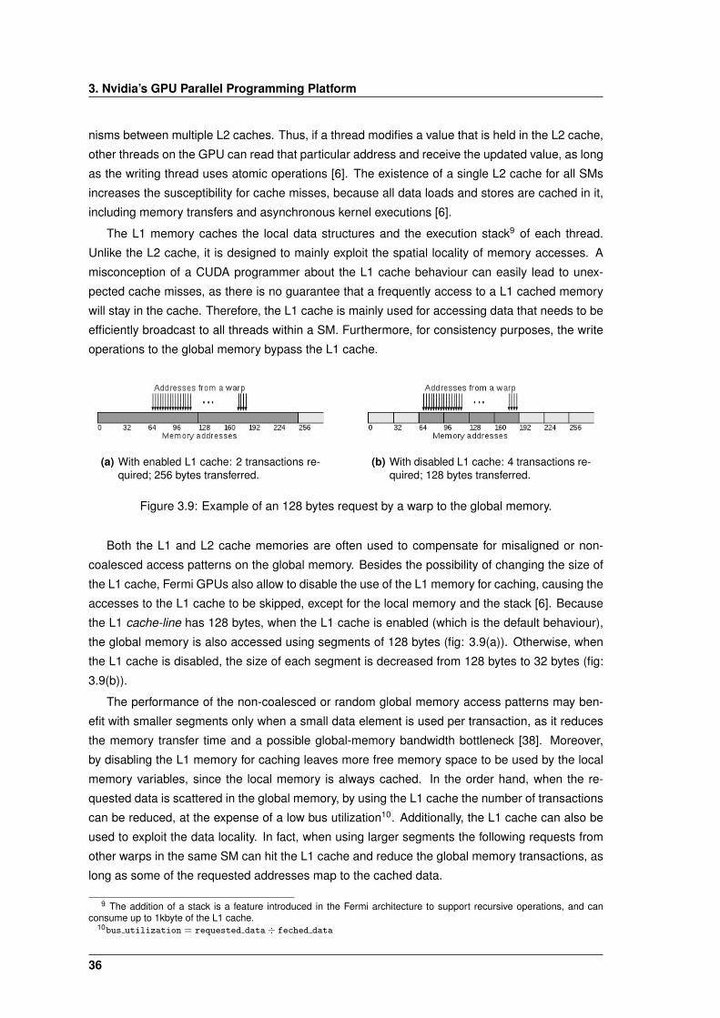
3. Nvidia’s GPU Parallel Programming Platform
nisms between multiple L2 caches. Thus, if a thread modifies a value that is held in the L2 cache,
other threads on the GPU can read that particular address and receive the updated value, as long
as the writing thread uses atomic operations [6]. The existence of a single L2 cache for all SMs
increases the susceptibility for cache misses, because all data loads and stores are cached in it,
including memory transfers and asynchronous kernel executions [6].
The L1 memory caches the local data structures and the execution stack9 of each thread.
Unlike the L2 cache, it is designed to mainly exploit the spatial locality of memory accesses. A
misconception of a CUDA programmer about the L1 cache behaviour can easily lead to unex-
pected cache misses, as there is no guarantee that a frequently access to a L1 cached memory
will stay in the cache. Therefore, the L1 cache is mainly used for accessing data that needs to be
efficiently broadcast to all threads within a SM. Furthermore, for consistency purposes, the write
operations to the global memory bypass the L1 cache.
(a) With enabled L1 cache: 2 transactions re-quired; 256 bytes transferred.
(b) With disabled L1 cache: 4 transactions re-quired; 128 bytes transferred.
Figure 3.9: Example of an 128 bytes request by a warp to the global memory.
Both the L1 and L2 cache memories are often used to compensate for misaligned or non-
coalesced access patterns on the global memory. Besides the possibility of changing the size of
the L1 cache, Fermi GPUs also allow to disable the use of the L1 memory for caching, causing the
accesses to the L1 cache to be skipped, except for the local memory and the stack [6]. Because
the L1 cache-line has 128 bytes, when the L1 cache is enabled (which is the default behaviour),
the global memory is also accessed using segments of 128 bytes (fig: 3.9(a)). Otherwise, when
the L1 cache is disabled, the size of each segment is decreased from 128 bytes to 32 bytes (fig:
3.9(b)).
The performance of the non-coalesced or random global memory access patterns may ben-
efit with smaller segments only when a small data element is used per transaction, as it reduces
the memory transfer time and a possible global-memory bandwidth bottleneck [38]. Moreover,
by disabling the L1 memory for caching leaves more free memory space to be used by the local
memory variables, since the local memory is always cached. In the order hand, when the re-
quested data is scattered in the global memory, by using the L1 cache the number of transactions
can be reduced, at the expense of a low bus utilization10. Additionally, the L1 cache can also be
used to exploit the data locality. In fact, when using larger segments the following requests from
other warps in the same SM can hit the L1 cache and reduce the global memory transactions, as
long as some of the requested addresses map to the cached data.
9 The addition of a stack is a feature introduced in the Fermi architecture to support recursive operations, and canconsume up to 1kbyte of the L1 cache.
10bus utilization = requested data÷ feched data
36
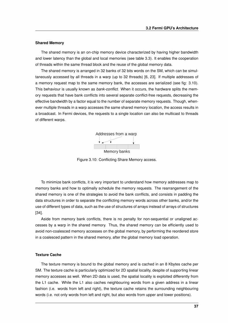
3.2 Fermi GPU’s Architecture
Shared Memory
The shared memory is an on-chip memory device characterized by having higher bandwidth
and lower latency than the global and local memories (see table 3.3). It enables the cooperation
of threads within the same thread block and the reuse of the global memory data.
The shared memory is arranged in 32 banks of 32 bits words on the SM, which can be simul-
taneously accessed by all threads in a warp (up to 32 threads) [6, 23]. If multiple addresses of
a memory request map to the same memory bank, the accesses are serialized (see fig: 3.10).
This behaviour is usually known as bank-conflict. When it occurs, the hardware splits the mem-
ory requests that have bank conflicts into several separate conflict-free requests, decreasing the
effective bandwidth by a factor equal to the number of separate memory requests. Though, when-
ever multiple threads in a warp accesses the same shared memory location, the access results in
a broadcast. In Fermi devices, the requests to a single location can also be multicast to threads
of different warps.
Figure 3.10: Conflicting Share Memory access.
To minimize bank conflicts, it is very important to understand how memory addresses map to
memory banks and how to optimally schedule the memory requests. The rearrangement of the
shared memory is one of the strategies to avoid the bank conflicts, and consists in padding the
data structures in order to separate the conflicting memory words across other banks, and/or the
use of different types of data, such as the use of structures of arrays instead of arrays of structures
[34].
Aside from memory bank conflicts, there is no penalty for non-sequential or unaligned ac-
cesses by a warp in the shared memory. Thus, the shared memory can be efficiently used to
avoid non-coalesced memory accesses on the global memory, by performing the reordered store
in a coalesced pattern in the shared memory, after the global memory load operation.
Texture Cache
The texture memory is bound to the global memory and is cached in an 8 Kbytes cache per
SM. The texture cache is particularly optimized for 2D spatial locality, despite of supporting linear
memory accesses as well. When 2D data is used, the spatial locality is exploited differently from
the L1 cache. While the L1 also caches neighbouring words from a given address in a linear
fashion (i.e. words from left and right), the texture cache retains the surrounding neighbouring
words (i.e. not only words from left and right, but also words from upper and lower positions).
37
3. Nvidia’s GPU Parallel Programming Platform
However, the texture cache is not kept coherent with respect to global memory writes within a
kernel execution, as texture cache fetches corresponding to addresses that have been written via
global stores in the same kernel call return undefined data. The coherency is only guaranteed for
write operations made by previous kernels or a previous memory copy operation in the host [23].
Fast Atomic Memory Operations
The conventional approach to provide an atomic operation, in a program executing on the host
usually consists in a two-step process, where a CPU uses an atomic test-and-set instruction to
manage a semaphore, which in turn manages the access to a predefined location in memory.
Unlike this software implementation in the host, Fermi devices use the ALU to directly perform
the atomic operation, rather than having to wait until a semaphore becomes available. The read-
modify-write atomic operations are implemented by locking the access to a single memory ad-
dress, until they are completed. This memory address can be located in different types of the
device’s memory subsystem, such as in the global memory or in the L2 cache subsystem. During
the lock interval, the rest of the memory continues to be available [8].
GigaThread Scheduler
The GigaThread Scheduler provides the means for a fast context switching, a concurrent ker-
nel execution and an improved thread block scheduling. In particular, the Fermi GPU architecture
features a two-level distributed thread scheduler. At a higher level, the device has a global work
distribution engine that schedules the thread blocks to various stream multiprocessors. At a lower
level, in the stream multiprocessor each warp scheduler distributes the warps of 32 threads to its
execution units.
The GigaThread hardware scheduler distributes the several thread blocks to the SMs accord-
ing the their available capacity, which dynamic balances the computing workload across the GPU.
It has the capability to manage 1536 simultaneously active threads for each SM across 16 kernels
[8, 19].
Regarding to the concurrent execution of kernels, and in order to maximise the GPU utiliza-
tion, each independent kernel of the same application context is issued to the unoccupied SMs,
until all have been fulfilled or the maximum number of supported concurrent kernels have been
achieved. Fermi GPUs support up to 16 different kernels of the same application context to exe-
cute concurrently [8, 20].
The implemented context switching mechanisms give support the GPU multitasking capa-
bilities, where each process is given a time slice of the processor’s resources. Fermi GPUs can
switch between applications in 25 microseconds, which is 20 times faster than previous-generation
GPUs [8]. This fast context switching is required to maintain a high utilization of the GPU, while
running multiple applications.
38
4Related Work
Contents4.1 Fast intra-prediction implementations based on General Purpose Proces-
sors (GPPs) . . . . . . . . . . . . . . . . . . . . . . . . . . . . . . . . . . . . . . 404.2 GPU implementation of H.264 Intra-Prediction . . . . . . . . . . . . . . . . . . 42
39
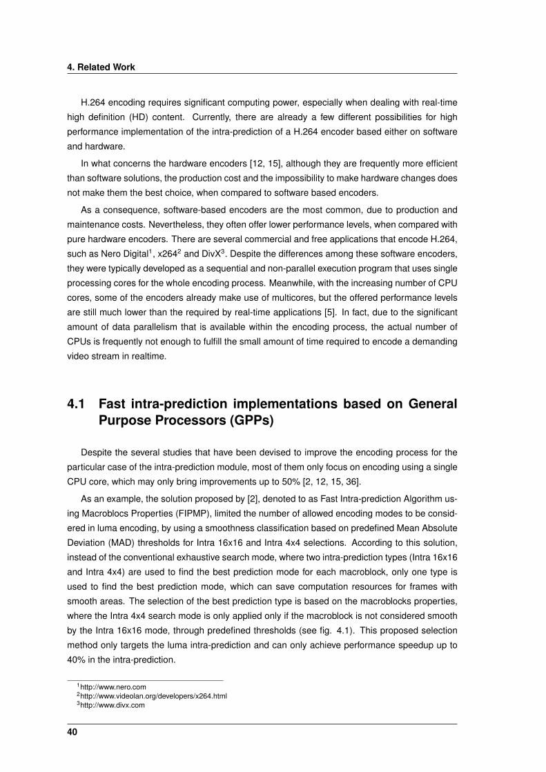
4. Related Work
H.264 encoding requires significant computing power, especially when dealing with real-time
high definition (HD) content. Currently, there are already a few different possibilities for high
performance implementation of the intra-prediction of a H.264 encoder based either on software
and hardware.
In what concerns the hardware encoders [12, 15], although they are frequently more efficient
than software solutions, the production cost and the impossibility to make hardware changes does
not make them the best choice, when compared to software based encoders.
As a consequence, software-based encoders are the most common, due to production and
maintenance costs. Nevertheless, they often offer lower performance levels, when compared with
pure hardware encoders. There are several commercial and free applications that encode H.264,
such as Nero Digital1, x2642 and DivX3. Despite the differences among these software encoders,
they were typically developed as a sequential and non-parallel execution program that uses single
processing cores for the whole encoding process. Meanwhile, with the increasing number of CPU
cores, some of the encoders already make use of multicores, but the offered performance levels
are still much lower than the required by real-time applications [5]. In fact, due to the significant
amount of data parallelism that is available within the encoding process, the actual number of
CPUs is frequently not enough to fulfill the small amount of time required to encode a demanding
video stream in realtime.
4.1 Fast intra-prediction implementations based on GeneralPurpose Processors (GPPs)
Despite the several studies that have been devised to improve the encoding process for the
particular case of the intra-prediction module, most of them only focus on encoding using a single
CPU core, which may only bring improvements up to 50% [2, 12, 15, 36].
As an example, the solution proposed by [2], denoted to as Fast Intra-prediction Algorithm us-
ing Macroblocs Properties (FIPMP), limited the number of allowed encoding modes to be consid-
ered in luma encoding, by using a smoothness classification based on predefined Mean Absolute
Deviation (MAD) thresholds for Intra 16x16 and Intra 4x4 selections. According to this solution,
instead of the conventional exhaustive search mode, where two intra-prediction types (Intra 16x16
and Intra 4x4) are used to find the best prediction mode for each macroblock, only one type is
used to find the best prediction mode, which can save computation resources for frames with
smooth areas. The selection of the best prediction type is based on the macroblocks properties,
where the Intra 4x4 search mode is only applied only if the macroblock is not considered smooth
by the Intra 16x16 mode, through predefined thresholds (see fig. 4.1). This proposed selection
method only targets the luma intra-prediction and can only achieve performance speedup up to
40% in the intra-prediction.
1http://www.nero.com2http://www.videolan.org/developers/x264.html3http://www.divx.com
40
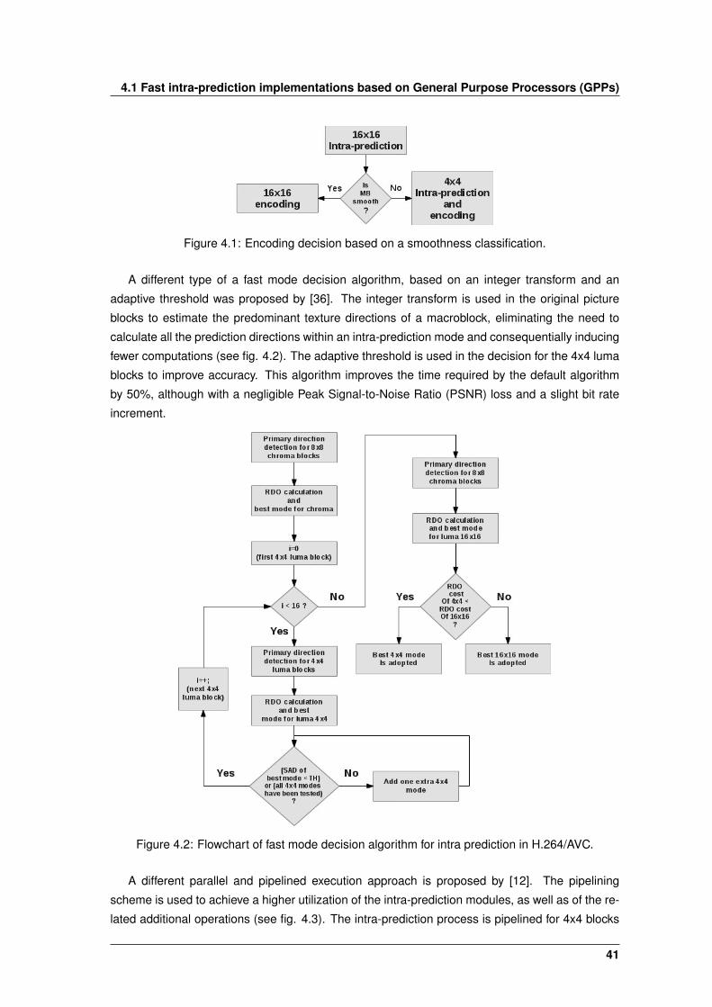
4.1 Fast intra-prediction implementations based on General Purpose Processors (GPPs)
Figure 4.1: Encoding decision based on a smoothness classification.
A different type of a fast mode decision algorithm, based on an integer transform and an
adaptive threshold was proposed by [36]. The integer transform is used in the original picture
blocks to estimate the predominant texture directions of a macroblock, eliminating the need to
calculate all the prediction directions within an intra-prediction mode and consequentially inducing
fewer computations (see fig. 4.2). The adaptive threshold is used in the decision for the 4x4 luma
blocks to improve accuracy. This algorithm improves the time required by the default algorithm
by 50%, although with a negligible Peak Signal-to-Noise Ratio (PSNR) loss and a slight bit rate
increment.
Figure 4.2: Flowchart of fast mode decision algorithm for intra prediction in H.264/AVC.
A different parallel and pipelined execution approach is proposed by [12]. The pipelining
scheme is used to achieve a higher utilization of the intra-prediction modules, as well as of the re-
lated additional operations (see fig. 4.3). The intra-prediction process is pipelined for 4x4 blocks
41
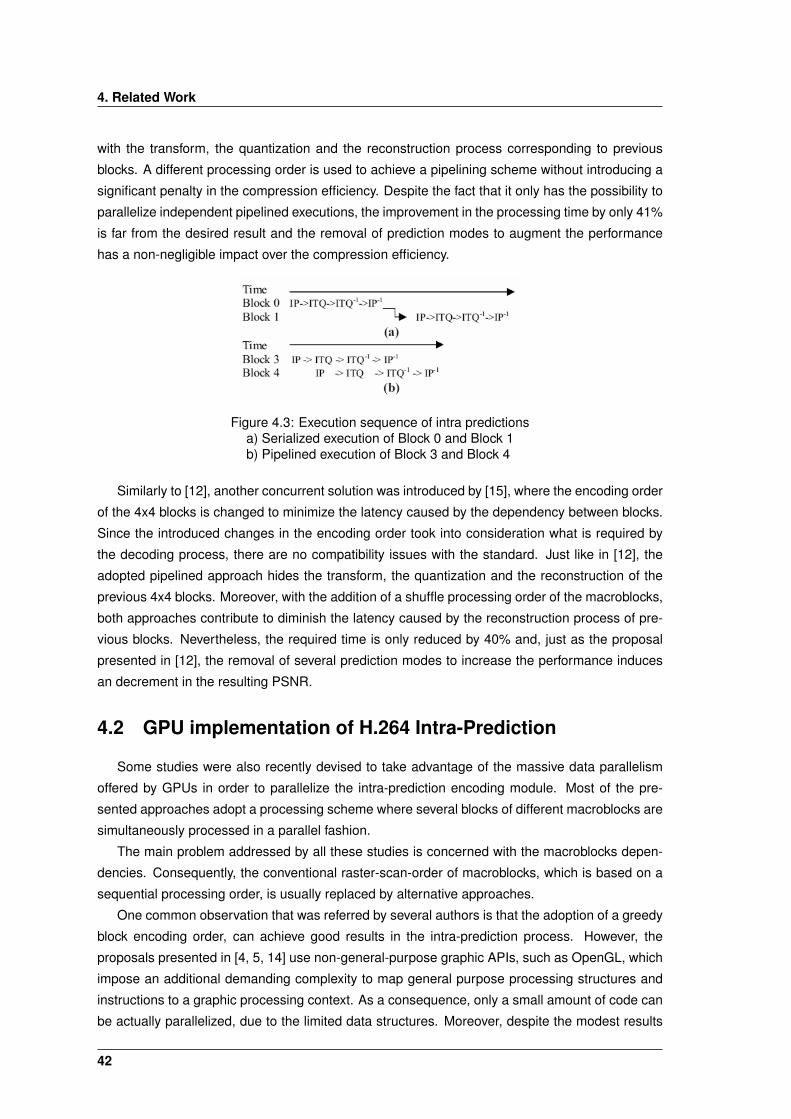
4. Related Work
with the transform, the quantization and the reconstruction process corresponding to previous
blocks. A different processing order is used to achieve a pipelining scheme without introducing a
significant penalty in the compression efficiency. Despite the fact that it only has the possibility to
parallelize independent pipelined executions, the improvement in the processing time by only 41%
is far from the desired result and the removal of prediction modes to augment the performance
has a non-negligible impact over the compression efficiency.
Figure 4.3: Execution sequence of intra predictionsa) Serialized execution of Block 0 and Block 1b) Pipelined execution of Block 3 and Block 4
Similarly to [12], another concurrent solution was introduced by [15], where the encoding order
of the 4x4 blocks is changed to minimize the latency caused by the dependency between blocks.
Since the introduced changes in the encoding order took into consideration what is required by
the decoding process, there are no compatibility issues with the standard. Just like in [12], the
adopted pipelined approach hides the transform, the quantization and the reconstruction of the
previous 4x4 blocks. Moreover, with the addition of a shuffle processing order of the macroblocks,
both approaches contribute to diminish the latency caused by the reconstruction process of pre-
vious blocks. Nevertheless, the required time is only reduced by 40% and, just as the proposal
presented in [12], the removal of several prediction modes to increase the performance induces
an decrement in the resulting PSNR.
4.2 GPU implementation of H.264 Intra-Prediction
Some studies were also recently devised to take advantage of the massive data parallelism
offered by GPUs in order to parallelize the intra-prediction encoding module. Most of the pre-
sented approaches adopt a processing scheme where several blocks of different macroblocks are
simultaneously processed in a parallel fashion.
The main problem addressed by all these studies is concerned with the macroblocks depen-
dencies. Consequently, the conventional raster-scan-order of macroblocks, which is based on a
sequential processing order, is usually replaced by alternative approaches.
One common observation that was referred by several authors is that the adoption of a greedy
block encoding order, can achieve good results in the intra-prediction process. However, the
proposals presented in [4, 5, 14] use non-general-purpose graphic APIs, such as OpenGL, which
impose an additional demanding complexity to map general purpose processing structures and
instructions to a graphic processing context. As a consequence, only a small amount of code can
be actually parallelized, due to the limited data structures. Moreover, despite the modest results
42
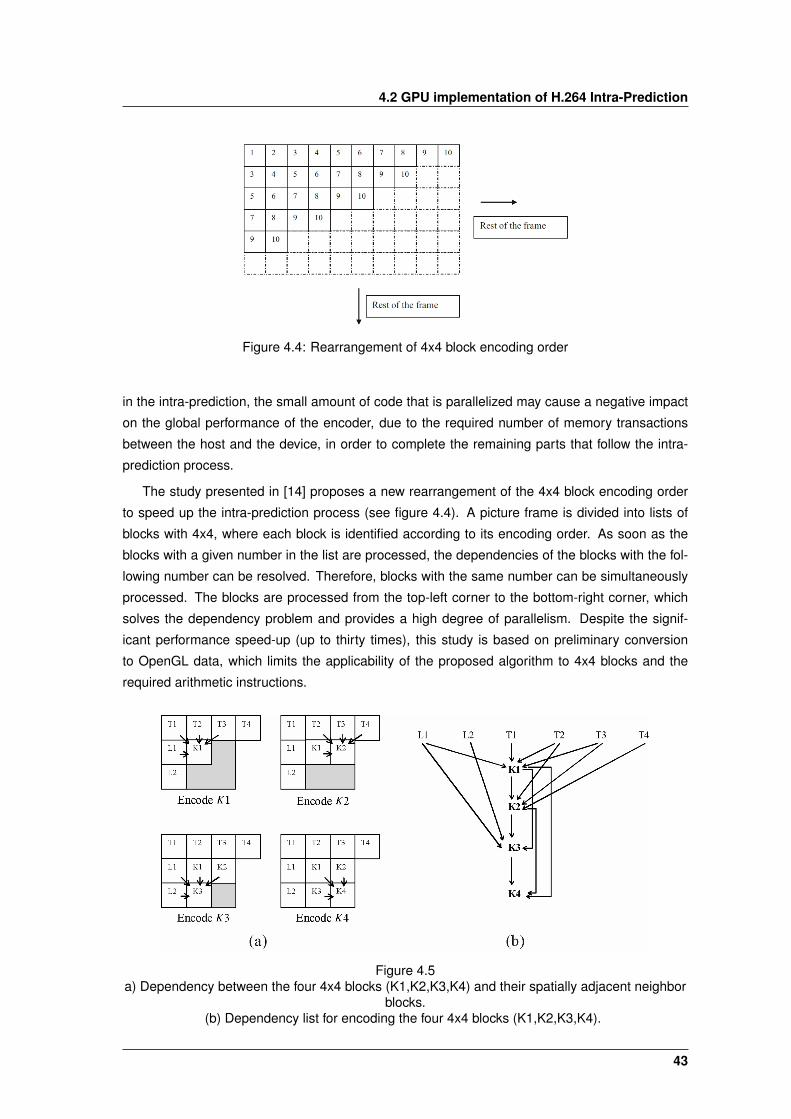
4.2 GPU implementation of H.264 Intra-Prediction
Figure 4.4: Rearrangement of 4x4 block encoding order
in the intra-prediction, the small amount of code that is parallelized may cause a negative impact
on the global performance of the encoder, due to the required number of memory transactions
between the host and the device, in order to complete the remaining parts that follow the intra-
prediction process.
The study presented in [14] proposes a new rearrangement of the 4x4 block encoding order
to speed up the intra-prediction process (see figure 4.4). A picture frame is divided into lists of
blocks with 4x4, where each block is identified according to its encoding order. As soon as the
blocks with a given number in the list are processed, the dependencies of the blocks with the fol-
lowing number can be resolved. Therefore, blocks with the same number can be simultaneously
processed. The blocks are processed from the top-left corner to the bottom-right corner, which
solves the dependency problem and provides a high degree of parallelism. Despite the signif-
icant performance speed-up (up to thirty times), this study is based on preliminary conversion
to OpenGL data, which limits the applicability of the proposed algorithm to 4x4 blocks and the
required arithmetic instructions.
Figure 4.5a) Dependency between the four 4x4 blocks (K1,K2,K3,K4) and their spatially adjacent neighbor
blocks.(b) Dependency list for encoding the four 4x4 blocks (K1,K2,K3,K4).
43
4. Related Work
Similarly, [4] proposes an alternate block encoding order to facilitate the Rate Distortion (RD)
cost computation in GPUs. The prediction direction is considered to derive the blocks dependency.
Unlike [14], instead of the usual raster-scan order, a greedy-based block encoding order is used
by defining directed acyclic graph (DAG) based on the dependency relationships to maximize the
parallelization in computing the RD cost at the GPU (see fig. 4.5). The blocks from different mac-
roblocks can be encoded in parallel, according to the dependency constrains of intra-prediction.
In each cycle, all blocks whose parents have already been encoded and whose reconstructed ref-
erence blocks are available can be immediately processed. Although the encoding of the blocks
is processed by using this greedy-based order, the output bitstream is organized according to the
raster-scan-ordering in order to conform to the H.264 standard. Despite demonstrating that their
solution is optimal and claiming a speed up to 80 times for high definition streams, the implemen-
tation process is the same as stated by [14].
44

5Solution Architecture
Contents5.1 Problem Partitioning . . . . . . . . . . . . . . . . . . . . . . . . . . . . . . . . . 465.2 Requisites and Constraints . . . . . . . . . . . . . . . . . . . . . . . . . . . . . 495.3 Architecture Design . . . . . . . . . . . . . . . . . . . . . . . . . . . . . . . . . . 505.4 Execution Model . . . . . . . . . . . . . . . . . . . . . . . . . . . . . . . . . . . . 68
45
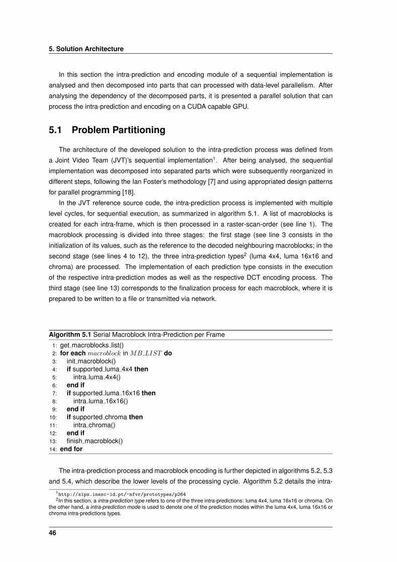
5. Solution Architecture
In this section the intra-prediction and encoding module of a sequential implementation is
analysed and then decomposed into parts that can processed with data-level parallelism. After
analysing the dependency of the decomposed parts, it is presented a parallel solution that can
process the intra-prediction and encoding on a CUDA capable GPU.
5.1 Problem Partitioning
The architecture of the developed solution to the intra-prediction process was defined from
a Joint Video Team (JVT)’s sequential implementation1. After being analysed, the sequential
implementation was decomposed into separated parts which were subsequently reorganized in
different steps, following the Ian Foster’s methodology [7] and using appropriated design patterns
for parallel programming [18].
In the JVT reference source code, the intra-prediction process is implemented with multiple
level cycles, for sequential execution, as summarized in algorithm 5.1. A list of macroblocks is
created for each intra-frame, which is then processed in a raster-scan-order (see line 1). The
macroblock processing is divided into three stages: the first stage (see line 3 consists in the
initialization of its values, such as the reference to the decoded neighbouring macroblocks; in the
second stage (see lines 4 to 12), the three intra-prediction types2 (luma 4x4, luma 16x16 and
chroma) are processed. The implementation of each prediction type consists in the execution
of the respective intra-prediction modes as well as the respective DCT encoding process. The
third stage (see line 13) corresponds to the finalization process for each macroblock, where it is
prepared to be written to a file or transmitted via network.
Algorithm 5.1 Serial Macroblock Intra-Prediction per Frame
1: get macroblocks list()2: for each macroblock in MB LIST do3: init macroblock()4: if supported luma 4x4 then5: intra luma 4x4()6: end if7: if supported luma 16x16 then8: intra luma 16x16()9: end if
10: if supported chroma then11: intra chroma()12: end if13: finish macroblock()14: end for
The intra-prediction process and macroblock encoding is further depicted in algorithms 5.2, 5.3
and 5.4, which describe the lower levels of the processing cycle. Algorithm 5.2 details the intra-
1http://sips.inesc-id.pt/~nfvr/prototypes/p2642In this section, a intra-prediction type refers to one of the three intra-predictions: luma 4x4, luma 16x16 or chroma. On
the other hand, a intra-prediction mode is used to denote one of the prediction modes within the luma 4x4, luma 16x16 orchroma intra-predictions types.
46
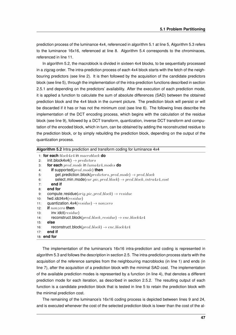
5.1 Problem Partitioning
prediction process of the luminance 4x4, referenced in algorithm 5.1 at line 5, Algorithm 5.3 refers
to the luminance 16x16, referenced at line 8. Algorithm 5.4 corresponds to the chrominaces,
referenced in line 11.
In algorithm 5.2, the macroblock is divided in sixteen 4x4 blocks, to be sequentially processed
in a zigzag order. The intra-prediction process of each 4x4 block starts with the fetch of the neigh-
bouring predictors (see line 2). It is then followed by the acquisition of the candidate predictors
block (see line 5), through the implementation of the intra-prediction functions described in section
2.5.1 and depending on the predictors’ availability. After the execution of each prediction mode,
it is applied a function to calculate the sum of absolute differences (SAD) between the obtained
prediction block and the 4x4 block in the current picture. The prediction block will persist or will
be discarded if it has or has not the minimum cost (see line 6). The following lines describe the
implementation of the DCT encoding process, which begins with the calculation of the residue
block (see line 9), followed by a DCT transform, quantization, inverse DCT transform and compu-
tation of the encoded block, which in turn, can be obtained by adding the reconstructed residue to
the prediction block, or by simply rebuilding the prediction block, depending on the output of the
quantization process.
Algorithm 5.2 Intra prediction and transform coding for luminance 4x4
1: for each block4x4 in macroblock do2: init block4x4()→ predictors3: for each pred mode in luma4x4 modes do4: if supported(pred mode) then5: get prediction block(predictors, pred mode)→ pred block6: select min mode(cur pic, pred block)→ pred block, intra4x4 cost7: end if8: end for9: compute residue(orig pic, pred block)→ residue
10: fwd idct4x4(residue)11: quantization 4x4(residue)→ nonzero12: if nonzero then13: inv idct(residue)14: reconstruct block(pred block, residue)→ enc block4x415: else16: reconstruct block(pred block)→ enc block4x417: end if18: end for
The implementation of the luminance’s 16x16 intra-prediction and coding is represented in
algorithm 5.3 and follows the description in section 2.5. The intra-prediction process starts with the
acquisition of the reference samples from the neighbouring macroblocks (in line 1) and ends (in
line 7), after the acquisition of a prediction block with the minimal SAD cost. The implementation
of the available prediction modes is represented by a function (in line 4), that denotes a different
prediction mode for each iteration, as described in section 2.5.2. The resulting output of each
function is a candidate prediction block that is tested in line 5 to retain the prediction block with
the minimal prediction cost.
The remaining of the luminance’s 16x16 coding process is depicted between lines 9 and 24,
and is executed whenever the cost of the selected prediction block is lower than the cost of the al-
47
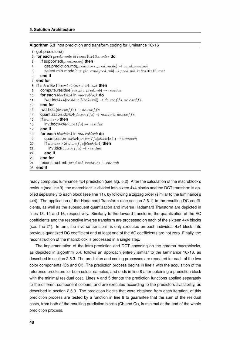
5. Solution Architecture
Algorithm 5.3 Intra prediction and transform coding for luminance 16x16
1: get predictors()2: for each pred mode in luma16x16 modes do3: if supported(pred mode) then4: get prediction mb(predictors, pred mode)→ cand pred mb5: select min mode(cur pic, candpred mb)→ pred mb, intra16x16 cost6: end if7: end for8: if intra16x16 cost < intra4x4 cost then9: compute residue(cur pic, pred mb)→ residue
10: for each block4x4 in macroblock do11: fwd idct4x4(residue[block4x4])→ dc coeffs, ac coeffs12: end for13: fwd hdct(dc coeffs)→ dc coeffs14: quantization dc4x4(dc coeffs)→ nonzero, dc coeffs15: if nonzero then16: inv hdct4x4(dc ceffs)→ residue17: end if18: for each block4x4 in macroblock do19: quantization ac4x4(ac coeffs[block4x4])→ nonzero20: if nonzero or dc ceffs[block4x4] then21: inv idct(ac coeffs)→ residue22: end if23: end for24: reconstruct mb(pred mb, residue)→ enc mb25: end if
ready computed luminance 4x4 prediction (see alg. 5.2). After the calculation of the macroblock’s
residue (see line 9), the macroblock is divided into sixten 4x4 blocks and the DCT transform is ap-
plied separately to each block (see line 11), by following a zigzag order (similar to the luminance’s
4x4). The application of the Hadamard Transform (see section 2.6.1) to the resulting DC coeffi-
cients, as well as the subsequent quantization and inverse Hadamard Transform are depicted in
lines 13, 14 and 16, respectively. Similarly to the forward transform, the quantization of the AC
coefficients and the respective inverse transform are processed on each of the sixteen 4x4 blocks
(see line 21). In turn, the inverse transform is only executed on each individual 4x4 block if its
previous quantized DC coefficient and at least one of the AC coefficients are not zero. Finally, the
reconstruction of the macroblock is processed in a single step.
The implementation of the intra-prediction and DCT encoding on the chroma macroblocks,
as depicted in algorithm 5.4, follows an approach entirely similar to the luminance 16x16, as
described in section 2.5.3. The prediction and coding processes are repeated for each of the two
color components (Cb and Cr). The prediction process begins in line 1 with the acquisition of the
reference predictors for both colour samples, and ends in line 8 after obtaining a prediction block
with the minimal residual cost. Lines 4 and 5 denote the prediction functions applied separately
to the different component colours, and are executed according to the predictors availability, as
described in section 2.5.3. The prediction blocks that were obtained from each iteration, of this
prediction process are tested by a function in line 6 to guarantee that the sum of the residual
costs, from both of the resulting prediction blocks (Cb and Cr), is minimal at the end of the whole
prediction process.
48
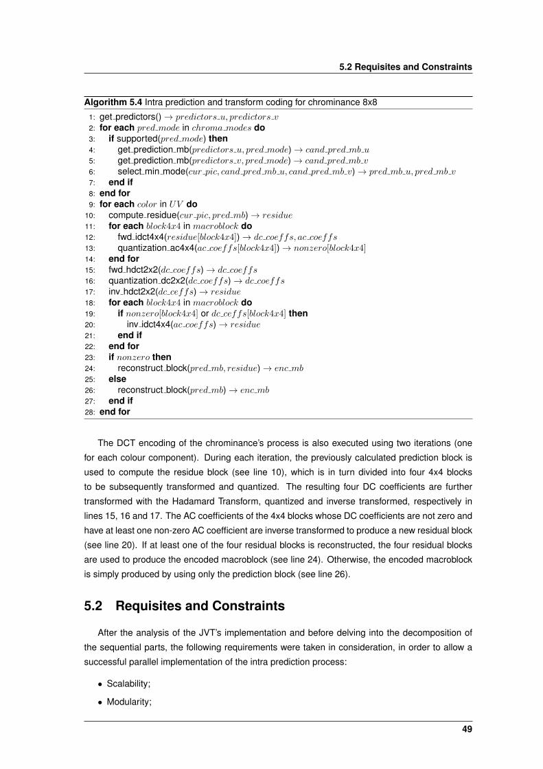
5.2 Requisites and Constraints
Algorithm 5.4 Intra prediction and transform coding for chrominance 8x8
1: get predictors()→ predictors u, predictors v2: for each pred mode in chroma modes do3: if supported(pred mode) then4: get prediction mb(predictors u, pred mode)→ cand pred mb u5: get prediction mb(predictors v, pred mode)→ cand pred mb v6: select min mode(cur pic, cand pred mb u, cand pred mb v)→ pred mb u, pred mb v7: end if8: end for9: for each color in UV do
10: compute residue(cur pic, pred mb)→ residue11: for each block4x4 in macroblock do12: fwd idct4x4(residue[block4x4])→ dc coeffs, ac coeffs13: quantization ac4x4(ac coeffs[block4x4])→ nonzero[block4x4]14: end for15: fwd hdct2x2(dc coeffs)→ dc coeffs16: quantization dc2x2(dc coeffs)→ dc coeffs17: inv hdct2x2(dc ceffs)→ residue18: for each block4x4 in macroblock do19: if nonzero[block4x4] or dc ceffs[block4x4] then20: inv idct4x4(ac coeffs)→ residue21: end if22: end for23: if nonzero then24: reconstruct block(pred mb, residue)→ enc mb25: else26: reconstruct block(pred mb)→ enc mb27: end if28: end for
The DCT encoding of the chrominance’s process is also executed using two iterations (one
for each colour component). During each iteration, the previously calculated prediction block is
used to compute the residue block (see line 10), which is in turn divided into four 4x4 blocks
to be subsequently transformed and quantized. The resulting four DC coefficients are further
transformed with the Hadamard Transform, quantized and inverse transformed, respectively in
lines 15, 16 and 17. The AC coefficients of the 4x4 blocks whose DC coefficients are not zero and
have at least one non-zero AC coefficient are inverse transformed to produce a new residual block
(see line 20). If at least one of the four residual blocks is reconstructed, the four residual blocks
are used to produce the encoded macroblock (see line 24). Otherwise, the encoded macroblock
is simply produced by using only the prediction block (see line 26).
5.2 Requisites and Constraints
After the analysis of the JVT’s implementation and before delving into the decomposition of
the sequential parts, the following requirements were taken in consideration, in order to allow a
successful parallel implementation of the intra prediction process:
• Scalability;
• Modularity;
49
5. Solution Architecture
• Concurrency;
• Performance;
• Locality;
• Determinism.
The scalability constrains must be met to guarantee that the implementation satisfies different
problems dimensions. Hence, an increase in the computing power will be sufficient to attain a
proportional increase in the problem size.
The modularity is a requirement that must be fulfilled in the design process and along the
whole implementation, to allow not only a good comprehension and interconnection of the different
problem parts to achieve the best solution as possible, but also to facilitate the development and
maintenance process.
The performance and concurrency are requirements that must be met to allow an efficient exe-
cution of each of the parallel executing parts, as well as an efficient mapping between the different
tasks and executions units. In an efficient implementation, the parallel tasks must be equally dis-
tributed across the execution units. Contrarily, an inefficient implementation is characterized by
an unbalanced distribution of tasks between execution units.
Concurrent tasks mainly process two types of data with different access costs: local data
and remote (or distributed) data. While the local data is predominantly processed by a single
task without the interference of other tasks, remote data requires mechanisms to distribute it
across several tasks and guarantee its correctness, thereby incurring more costly operations for
its access. Consequently, locality is a property that promotes the separation of local and remote
data in the case that local data is more frequently accessed than the remote data.
Lastly, a deterministic solution should guarantee the correctness of the execution, in that a
particular input always yields to the same output. Although a parallel implementation could tol-
erate non-deterministic executions, the deterministic behaviour is a desirable feature, especially
for debugging purposes, which could be hardened with a non-deterministic execution of multiple
concurrent tasks.
5.3 Architecture Design
After the enumeration of the main requisites, the design of the solution is obtained by following
the Foster’s methodology [7] for designing parallel programs, which consists in the adoption of a
group of steps that take into account the concurrency, scalability, locality and modularity requisites
in the parallel algorithms design. Foster’s methodology structures the design process as four
distinct phases:
1. Partitioning;
2. Communication;
3. Agglomeration;
4. Mapping.
50

5.3 Architecture Design
The first two stages focus on concurrency and scalability, and the remaining to locality and
other issues related to performance. In the following, the application of each of these phases to
this particular solution design will be further described, by using the parallel programming patterns
from [18].
5.3.1 Partitioning
The partitioning consists in the decomposition of the computation and of the data operations
into small tasks to recognize the opportunities for parallel execution. The decomposition allows to
identify and correctly manage the dependencies among tasks in order to avoid non-deterministic
issues. A fine-grained decomposition provides the greatest flexibility in terms of potential par-
allel algorithms. Hence, a large number of small tasks must be defined to yield a fine-grained
decomposition of the problem.
The focus of the decomposition can be oriented either to the data associated with the problem
or to the computation. The former approach is denoted by domain decomposition and consists
in dividing the data into small pieces and in partitioning the computation by associating each
operation with the data on which it operates. The alternative approach, denoted by functional
decomposition, has its focus on the computation rather than the data to be manipulated. It consists
in the division of the computation into small tasks and then associating the data to each task
[7, 18].
The functional and data decomposition approaches are complementary, as the function de-
composition is often followed by a data decomposition and vice-versa. In fact, the order of these
approaches may influence the solution design and hide or expose different parallel issues, as the
decomposition of tasks may hide important data structures, and the decomposition of data may
hide important tasks.
Despite the simplicity of the task-based algorithms [18], they are only efficient if each process-
ing element has access to a large memory with insignificant latency overhead. On the other hand,
an algorithm driven by a data-decomposition can make an efficient use of memory and minimize
the network bandwidth, but at the cost of more communication overhead during the concurrent
part of the computation. Hence, the partitioning should focus both on the computation associated
with a problem and on the data on which this computation operates, regardless of the approach
taken as the starting point. In fact, by analysing the algorithms 5.2, 5.3 and 5.4 it can be observed
that the serial implementation not only comprises several tasks of different granularities, where
a tasks correspond the a method call, but also these tasks operate on large data structures in
the presence of several macroblocks, allowing the exploitation of both the concurrent execution of
tasks and the concurrent processing on independent groups of data.
In the following, in order to avoid the limitations of a single decomposition approach, both
decomposition patterns will be considered. However, unlike the approach suggested by [7], where
the first decomposition approach drives the second approach (i.e: decomposing tasks based on
the data decomposition and vice-versa), both approaches are independently implemented and
the decomposed data structures are then mapped to the decomposed tasks.
51
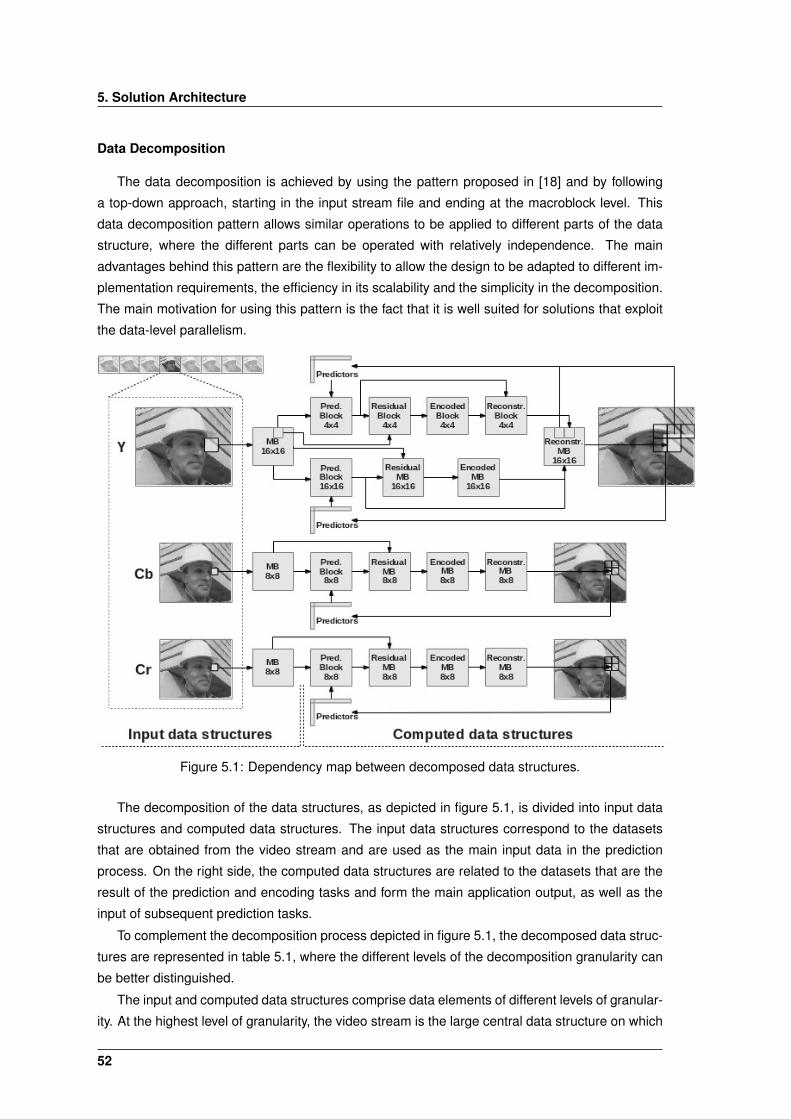
5. Solution Architecture
Data Decomposition
The data decomposition is achieved by using the pattern proposed in [18] and by following
a top-down approach, starting in the input stream file and ending at the macroblock level. This
data decomposition pattern allows similar operations to be applied to different parts of the data
structure, where the different parts can be operated with relatively independence. The main
advantages behind this pattern are the flexibility to allow the design to be adapted to different im-
plementation requirements, the efficiency in its scalability and the simplicity in the decomposition.
The main motivation for using this pattern is the fact that it is well suited for solutions that exploit
the data-level parallelism.
Figure 5.1: Dependency map between decomposed data structures.
The decomposition of the data structures, as depicted in figure 5.1, is divided into input data
structures and computed data structures. The input data structures correspond to the datasets
that are obtained from the video stream and are used as the main input data in the prediction
process. On the right side, the computed data structures are related to the datasets that are the
result of the prediction and encoding tasks and form the main application output, as well as the
input of subsequent prediction tasks.
To complement the decomposition process depicted in figure 5.1, the decomposed data struc-
tures are represented in table 5.1, where the different levels of the decomposition granularity can
be better distinguished.
The input and computed data structures comprise data elements of different levels of granular-
ity. At the highest level of granularity, the video stream is the large central data structure on which
52
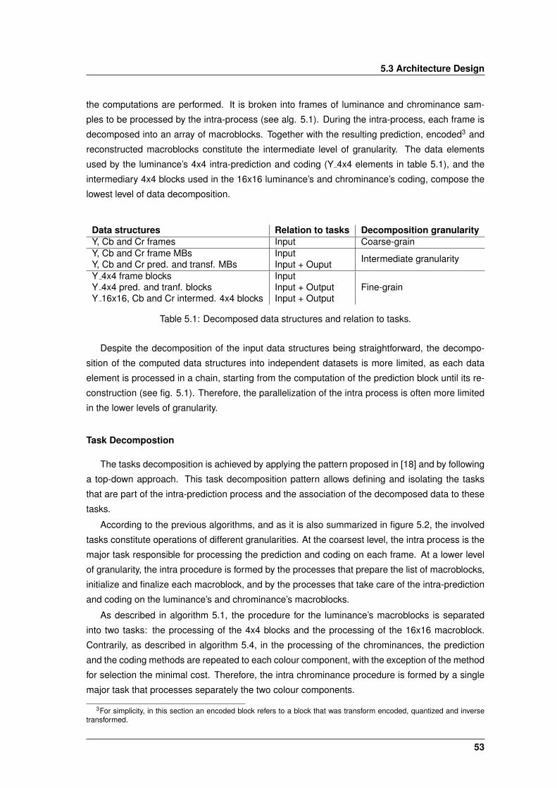
5.3 Architecture Design
the computations are performed. It is broken into frames of luminance and chrominance sam-
ples to be processed by the intra-process (see alg. 5.1). During the intra-process, each frame is
decomposed into an array of macroblocks. Together with the resulting prediction, encoded3 and
reconstructed macroblocks constitute the intermediate level of granularity. The data elements
used by the luminance’s 4x4 intra-prediction and coding (Y 4x4 elements in table 5.1), and the
intermediary 4x4 blocks used in the 16x16 luminance’s and chrominance’s coding, compose the
lowest level of data decomposition.
Data structures Relation to tasks Decomposition granularityY, Cb and Cr frames Input Coarse-grainY, Cb and Cr frame MBs Input Intermediate granularityY, Cb and Cr pred. and transf. MBs Input + OuputY 4x4 frame blocks Input
Fine-grainY 4x4 pred. and tranf. blocks Input + OutputY 16x16, Cb and Cr intermed. 4x4 blocks Input + Output
Table 5.1: Decomposed data structures and relation to tasks.
Despite the decomposition of the input data structures being straightforward, the decompo-
sition of the computed data structures into independent datasets is more limited, as each data
element is processed in a chain, starting from the computation of the prediction block until its re-
construction (see fig. 5.1). Therefore, the parallelization of the intra process is often more limited
in the lower levels of granularity.
Task Decompostion
The tasks decomposition is achieved by applying the pattern proposed in [18] and by following
a top-down approach. This task decomposition pattern allows defining and isolating the tasks
that are part of the intra-prediction process and the association of the decomposed data to these
tasks.
According to the previous algorithms, and as it is also summarized in figure 5.2, the involved
tasks constitute operations of different granularities. At the coarsest level, the intra process is the
major task responsible for processing the prediction and coding on each frame. At a lower level
of granularity, the intra procedure is formed by the processes that prepare the list of macroblocks,
initialize and finalize each macroblock, and by the processes that take care of the intra-prediction
and coding on the luminance’s and chrominance’s macroblocks.
As described in algorithm 5.1, the procedure for the luminance’s macroblocks is separated
into two tasks: the processing of the 4x4 blocks and the processing of the 16x16 macroblock.
Contrarily, as described in algorithm 5.4, in the processing of the chrominances, the prediction
and the coding methods are repeated to each colour component, with the exception of the method
for selection the minimal cost. Therefore, the intra chrominance procedure is formed by a single
major task that processes separately the two colour components.
3For simplicity, in this section an encoded block refers to a block that was transform encoded, quantized and inversetransformed.
53
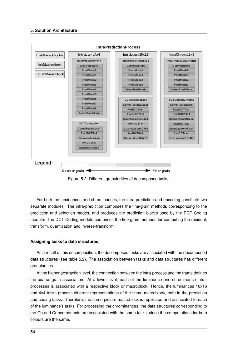
5. Solution Architecture
Figure 5.2: Different granularities of decomposed tasks.
For both the luminances and chrominances, the intra-prediction and encoding constitute two
separate modules. The intra-prediction comprises the fine-grain methods corresponding to the
prediction and selection modes, and produces the prediction blocks used by the DCT Coding
module. The DCT Coding module comprises the fine-grain methods for computing the residual,
transform, quantization and inverse-transform.
Assigning tasks to data structures
As a result of this decomposition, the decomposed tasks are associated with the decomposed
data structures (see table 5.2). The association between tasks and data structures has different
granularities.
At the higher abstraction level, the connection between the intra-process and the frame defines
the coarse-grain association. At a lower level, each of the luminance and chrominance intra-
processes is associated with a respective block or macroblock. Hence, the luminances 16x16
and 4x4 tasks process different representations of the same macroblock, both in the prediction
and coding tasks. Therefore, the same picture macroblock is replicated and associated to each
of the luminance’s tasks. For processing the chrominances, the data structures corresponding to
the Cb and Cr components are associated with the same tasks, since the computations for both
colours are the same.
54
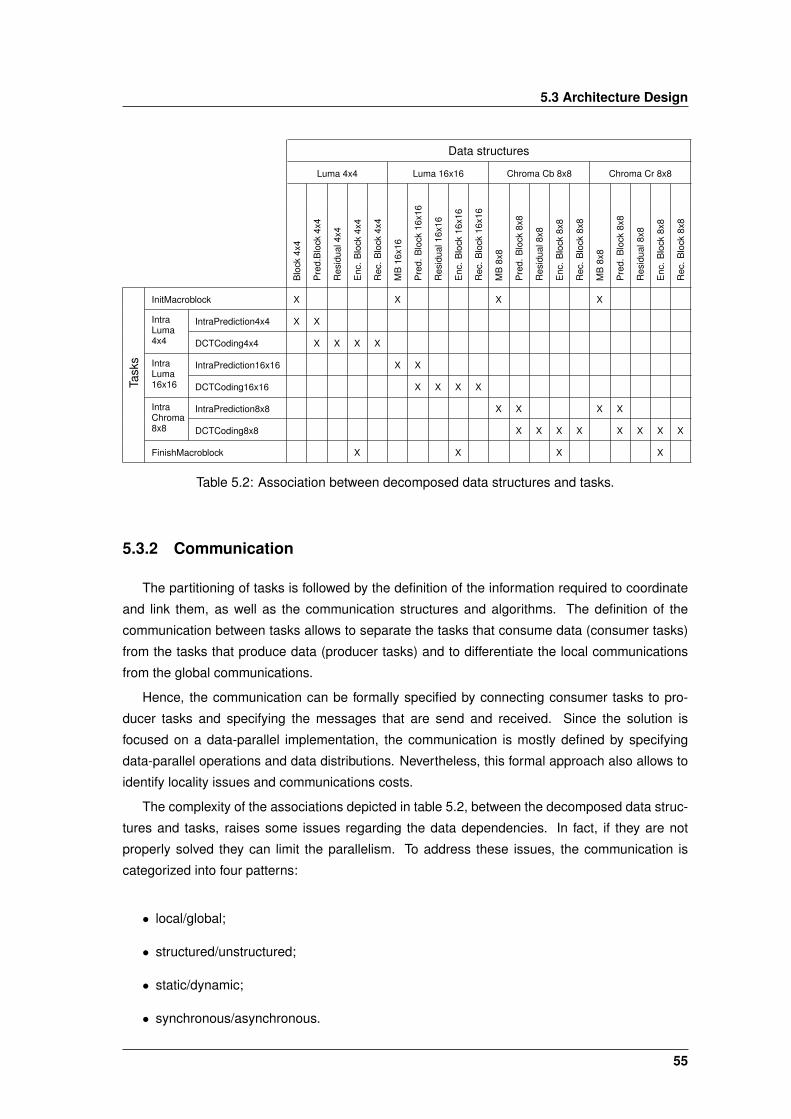
5.3 Architecture Design
Data structures
Luma 4x4 Luma 16x16 Chroma Cb 8x8 Chroma Cr 8x8
Blo
ck4x
4
Pre
d.B
lock
4x4
Res
idua
l4x4
Enc
.B
lock
4x4
Rec
.B
lock
4x4
MB
16x1
6
Pre
d.B
lock
16x1
6
Res
idua
l16x
16
Enc
.B
lock
16x1
6
Rec
.B
lock
16x1
6
MB
8x8
Pre
d.B
lock
8x8
Res
idua
l8x8
Enc
.B
lock
8x8
Rec
.B
lock
8x8
MB
8x8
Pre
d.B
lock
8x8
Res
idua
l8x8
Enc
.B
lock
8x8
Rec
.B
lock
8x8
Task
s
InitMacroblock X X X X
IntraLuma4x4
IntraPrediction4x4 X X
DCTCoding4x4 X X X X
IntraLuma16x16
IntraPrediction16x16 X X
DCTCoding16x16 X X X X
IntraChroma8x8
IntraPrediction8x8 X X X X
DCTCoding8x8 X X X X X X X X
FinishMacroblock X X X X
Table 5.2: Association between decomposed data structures and tasks.
5.3.2 Communication
The partitioning of tasks is followed by the definition of the information required to coordinate
and link them, as well as the communication structures and algorithms. The definition of the
communication between tasks allows to separate the tasks that consume data (consumer tasks)
from the tasks that produce data (producer tasks) and to differentiate the local communications
from the global communications.
Hence, the communication can be formally specified by connecting consumer tasks to pro-
ducer tasks and specifying the messages that are send and received. Since the solution is
focused on a data-parallel implementation, the communication is mostly defined by specifying
data-parallel operations and data distributions. Nevertheless, this formal approach also allows to
identify locality issues and communications costs.
The complexity of the associations depicted in table 5.2, between the decomposed data struc-
tures and tasks, raises some issues regarding the data dependencies. In fact, if they are not
properly solved they can limit the parallelism. To address these issues, the communication is
categorized into four patterns:
• local/global;
• structured/unstructured;
• static/dynamic;
• synchronous/asynchronous.
55
5. Solution Architecture
Local Communication
Local communication is related with the exchange of information between a small group of
tasks and concerns the finer-grained tasks of the intra-prediction process. In each intra-prediction
module (see fig. 5.2) the fine-grain tasks that select the best prediction modes communicate with
the tasks that compute the prediction modes. In the DCT coding modules, each task is processed
in order, starting from the computation of the residual to the block reconstruction and passing the
computed data to the next task.
Global Communication
Global communication operations include the participation of many tasks. Typically, when an
operation requires the communication between a large group of tasks, it usually rises two kinds of
problems that can hinder the parallel performance: centralization of the execution, which avoids
the distribution of computation and communication, by using one task to coordinate the com-
munications; and sequential execution, which avoids multiple computations and communication
operations to proceed concurrently.
Because each frame is separated into macroblocks, a significant amount of communication
channels are found between the fine-grain tasks, thereby being local. Hence, the global commu-
nication is irrelevant inside the intra-frame processing.
Structured/Unstructured and Static/Dynamic Communications
In structured communication, the tasks form a regular structure, such as a grid or a tree. The
unstructured communication is characterized by an irregular network structure, such as arbitrary
graphs. The communication is said to be static if the identity of the communication partners does
not change over time. Otherwise, if the communication structures may be determined by data that
is computed at runtime and are variable, the communication is considered dynamic.
Despite the macroblocks being organized in a fixed grid, in the intra-prediction process, the
variable number of neighbouring macroblocks causes a different execution of prediction modes.
This causes the number of communication channels between the tasks that selects the mini-
mal prediction mode and the tasks that compute the prediction blocks to vary along the time.
Therefore, the communication between the intra-prediction fine-grained tasks is considered un-
structured and dynamic. The communication among the remaining parts of the intra process can
be characterized as structured and static.
Synchronous/Asynchronous Communication
When using a synchronous communication model, both the producer and the consumer are
aware when the communication operations are required and the producer tasks explicitly send
data to the consumer tasks. Contrarily, when using asynchronous communication, the consumer
tasks must explicitly request data from the producer tasks.
The fine-grained tasks of the intra-process mainly communicate by sharing data, where each
task is executed in order and has the exclusive access to the shared data during its execution.
56
5.3 Architecture Design
Hence, the data-sharing model can be seen as a synchronous communication, where a tasks
assumes the role of a consumer when accessing the shared-data for reading and the role of a
producer when modifing the shared-data.
In the coarse-grained intra-process, the tasks that operate separately on each frame to re-
quest the picture frame, and that precede the remaining computations, can be characterized
as an asynchronous operation. Although each frame is sequentially read from the file-system,
many intra-process tasks may operate concurrently, due to the absence of dependencies between
frames.
Shared Data
The characterization of the communication patterns defines the relation between the decom-
posed data elements and the decomposed tasks to exploit the concurrent execution of tasks. Al-
though the shared data is implicitly integrated in the previous communication patterns, it is more
described with further detail, since the parallel implementation is mainly focused on an approach
that exploits the data parallelism the most part of the communication between tasks is thereby
based on a shared-memory model.
To identify the data that is shared among the groups of tasks and to manage the access to
the shared data in a correct and efficient way, the data sharing pattern from [18] is applied to
the decomposed data structures and tasks. By using this data sharing pattern, the incorrect data
accesses that lead to race conditions are avoided and the availability of the data elements is en-
sured with a minimum overhead introduced by excessive synchronization with barrier operations
[18]. This data sharing pattern separates the shared data into three categories:
• Read-only;
• Effectively-local;
• Read-write.
Because the intra-process is composed by an hierarchy of different granularities, the catego-
rization of the decomposed data elements varies depending on the context where it is accessed.
For example, one data structure can be defined as read-only by a group of tasks belonging to
a fine-grained context, but can be written by a different group of tasks that belongs to coarser-
grained context.
In particular, the shared data falls into the read-only category when it is only used for reading
purposes. The read-only data elements do not need to be protected against race conditions. In
figure 5.3, it is represented the relation between the intra-prediction procedure and related coding
tasks and the respective shared data elements. Only the frame macroblocks belong to the read-
only category, despite of the previous pre-processing by the initialization task (InitMacroblock).
Nevertheless, the frame macroblocks can be replicated across all tasks in order to exploit the
performance by using local data.
The effective-local category targets the data elements that are partitioned into subsets and
used (for read or write) by only one of the tasks. In the frame’s intra-prediction and coding con-
text, all the data structures are broken into blocks and macroblocks to be separately processed,
57
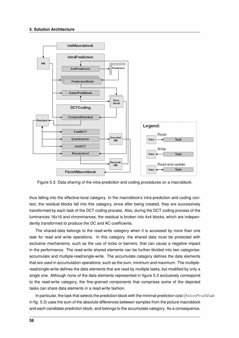
5. Solution Architecture
Figure 5.3: Data sharing of the intra-prediction and coding procedures on a macroblock.
thus falling into the effective-local category. In the macroblock’s intra-prediction and coding con-
text, the residual blocks fall into this category, since after being created, they are successively
transformed by each task of the DCT coding process. Also, during the DCT coding process of the
luminances 16x16 and chrominances, the residual is broken into 4x4 blocks, which are indepen-
dently transformed to produce the DC and AC coefficients.
The shared-data belongs to the read-write category when it is accessed by more than one
task for read and write operations. In this category, the shared data must be protected with
exclusive mechanisms, such as the use of locks or barriers, that can cause a negative impact
in the performance. The read-write shared elements can be further divided into two categories:
accumulate and multiple-read/single-write. The accumulate category defines the data elements
that are used in accumulation operations, such as the sum, minimum and maximum. The multiple-
read/single-write defines the data elements that are read by multiple tasks, but modified by only a
single one. Although none of the data elements represented in figure 5.3 exclusively correspond
to the read-write category, the fine-grained components that comprises some of the depicted
tasks can share data elements in a read-write fashion.
In particular, the task that selects the prediction block with the minimal prediction cost (SelectPredMode
in fig. 5.3) uses the sum of the absolute differences between samples from the picture macroblock
and each candidate prediction block, and belongs to the accumulate category. As a consequence,
58
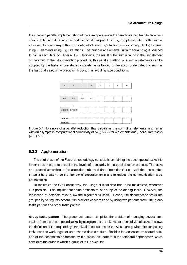
5.3 Architecture Design
the incorrect parallel implementation of the sum operation with shared data can lead to race con-
ditions. In figure 5.4 it is represented a conventional parallel O(log n) implementation of the sum of
all elements in an array with n elements, which uses m/2 tasks (number of grey blocks) for sum-
ming m elements using log n iterations. The number of elements (initially equal to n) is reduced
to half in each iteration. After all log n iterations, the result of the sum is found in the first element
of the array. In the intra-prediction procedure, this parallel method for summing elements can be
adopted by the tasks whose shared data elements belong to the accumulate category, such as
the task that selects the prediction blocks, thus avoiding race conditions.
Figure 5.4: Example of a parallel reduction that calculates the sum of all elements in an arraywith an asymptotic computational complexity of O( n
2p log n) for n elements and p concurrent tasks(p = 1/2n).
5.3.3 Agglomeration
The third phase of the Foster’s methodology consists in combining the decomposed tasks into
larger ones in order to establish the levels of granularity in the parallelization process. The tasks
are grouped according to the execution order and data dependencies to avoid that the number
of tasks be greater than the number of execution units and to reduce the communication costs
among tasks.
To maximize the GPU occupancy, the usage of local data has to be maximized, whenever
it is possible. This implies that some datasets must be replicated among tasks. However, the
replication of datasets must allow the algorithm to scale. Hence, the decomposed tasks are
grouped by taking into account the previous concerns and by using two patterns from [18]: group
tasks pattern and order tasks pattern.
Group tasks pattern The group task pattern simplifies the problem of managing several con-
straints from the decomposed tasks, by using groups of tasks rather than individual tasks. It allows
the definition of the required synchronization operations for the whole group when the composing
tasks need to work together on a shared data structure. Besides the accesses on shared data,
one of the constraints addressed by the group task pattern is the temporal dependency, which
considers the order in which a group of tasks executes.
59
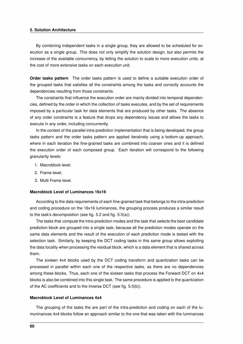
5. Solution Architecture
By combining independent tasks in a single group, they are allowed to be scheduled for ex-
ecution as a single group. This does not only simplify the solution design, but also permits the
increase of the available concurrency, by letting the solution to scale to more execution units, at
the cost of more extensive tasks on each execution unit.
Order tasks pattern The order tasks pattern is used to define a suitable execution order of
the grouped tasks that satisfies all the constraints among the tasks and correctly accounts the
dependencies resulting from those constraints.
The constraints that influence the execution order are mainly divided into temporal dependen-
cies, defined by the order in which the collection of tasks executes, and by the set of requirements
imposed by a particular task for data elements that are produced by other tasks. The absence
of any order constraints is a feature that drops any dependency issues and allows the tasks to
execute in any order, including concurrently.
In the context of the parallel intra-prediction implementation that is being developed, the group
tasks pattern and the order tasks pattern are applied iteratively using a bottom-up approach,
where in each iteration the fine-grained tasks are combined into coarser ones and it is defined
the execution order of each composed group. Each iteration will correspond to the following
granularity levels:
1. Macroblock level;
2. Frame level;
3. Multi Frame level.
Macroblock Level of Luminances 16x16
According to the data requirements of each fine-grained task that belongs to the intra-prediction
and coding procedure on the 16x16 luminances, the grouping process produces a similar result
to the task’s decomposition (see fig. 5.2 and fig. 5.5(a)).
The tasks that compute the intra-prediction modes and the task that selects the best candidate
prediction block are grouped into a single task, because all the prediction modes operate on the
same data elements and the result of the execution of each prediction mode is tested with the
selection task. Similarly, by keeping the DCT coding tasks in this same group allows exploiting
the data locality when processing the residual block, which is a data element that is shared across
them.
The sixteen 4x4 blocks used by the DCT coding transform and quantization tasks can be
processed in parallel within each one of the respective tasks, as there are no dependencies
among these blocks. Thus, each one of the sixteen tasks that process the Forward DCT on 4x4
blocks is also be combined into this single task. The same procedure is applied to the quantization
of the AC coefficients and to the Inverse DCT (see fig. 5.5(b)).
Macroblock Level of Luminances 4x4
The grouping of the tasks the are part of the intra-prediction and coding on each of the lu-
muninances 4x4 blocks follow an approach similar to the one that was taken with the luminances
60
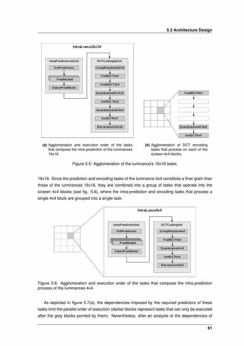
5.3 Architecture Design
(a) Agglomeration and execution order of the tasksthat compose the intra-prediction of the luminances16x16.
(b) Agglomeration of DCT encodingtasks that process on each of thesixteen 4x4 blocks.
Figure 5.5: Agglomeration of the luminance’s 16x16 tasks.
16x16. Since the prediction and encoding tasks of the luminance 4x4 constitute a finer grain than
those of the luminances 16x16, they are combined into a group of tasks that operate into the
sixteen 4x4 blocks (see fig. 5.6), where the intra-prediction and encoding tasks that process a
single 4x4 block are grouped into a single task.
Figure 5.6: Agglomeration and execution order of the tasks that compose the intra-predictionprocess of the luminances 4x4.
As depicted in figure 5.7(a), the dependencies imposed by the required predictors of these
tasks limit the parallel order of execution (darker blocks represent tasks that can only be executed
after the grey blocks pointed by them). Nevertheless, after an analysis of the dependencies of
61
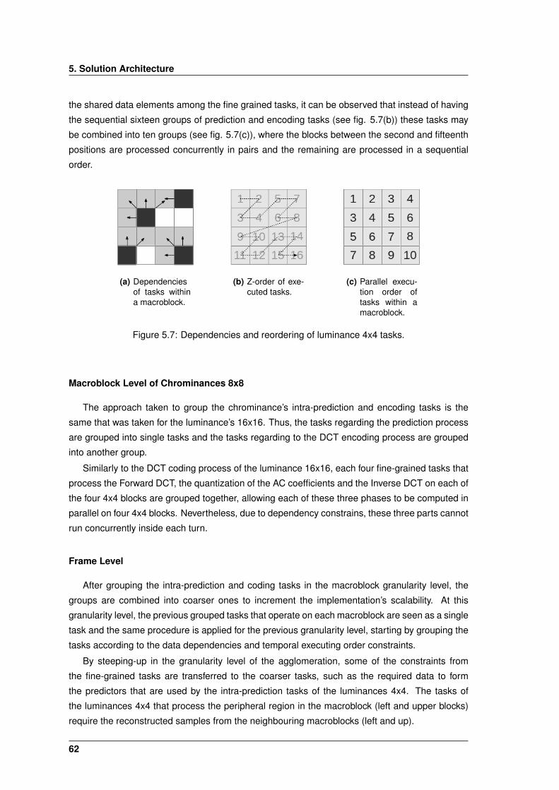
5. Solution Architecture
the shared data elements among the fine grained tasks, it can be observed that instead of having
the sequential sixteen groups of prediction and encoding tasks (see fig. 5.7(b)) these tasks may
be combined into ten groups (see fig. 5.7(c)), where the blocks between the second and fifteenth
positions are processed concurrently in pairs and the remaining are processed in a sequential
order.
(a) Dependenciesof tasks withina macroblock.
(b) Z-order of exe-cuted tasks.
(c) Parallel execu-tion order oftasks within amacroblock.
Figure 5.7: Dependencies and reordering of luminance 4x4 tasks.
Macroblock Level of Chrominances 8x8
The approach taken to group the chrominance’s intra-prediction and encoding tasks is the
same that was taken for the luminance’s 16x16. Thus, the tasks regarding the prediction process
are grouped into single tasks and the tasks regarding to the DCT encoding process are grouped
into another group.
Similarly to the DCT coding process of the luminance 16x16, each four fine-grained tasks that
process the Forward DCT, the quantization of the AC coefficients and the Inverse DCT on each of
the four 4x4 blocks are grouped together, allowing each of these three phases to be computed in
parallel on four 4x4 blocks. Nevertheless, due to dependency constrains, these three parts cannot
run concurrently inside each turn.
Frame Level
After grouping the intra-prediction and coding tasks in the macroblock granularity level, the
groups are combined into coarser ones to increment the implementation’s scalability. At this
granularity level, the previous grouped tasks that operate on each macroblock are seen as a single
task and the same procedure is applied for the previous granularity level, starting by grouping the
tasks according to the data dependencies and temporal executing order constraints.
By steeping-up in the granularity level of the agglomeration, some of the constraints from
the fine-grained tasks are transferred to the coarser tasks, such as the required data to form
the predictors that are used by the intra-prediction tasks of the luminances 4x4. The tasks of
the luminances 4x4 that process the peripheral region in the macroblock (left and upper blocks)
require the reconstructed samples from the neighbouring macroblocks (left and up).
62
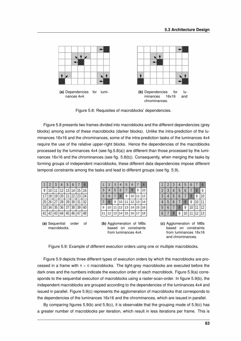
5.3 Architecture Design
(a) Dependencies for lumi-nances 4x4.
(b) Dependencies for lu-minances 16x16 andchrominances.
Figure 5.8: Requisites of macroblocks’ dependencies.
Figure 5.8 presents two frames divided into macroblocks and the different dependencies (grey
blocks) among some of these macroblocks (darker blocks). Unlike the intra-prediction of the lu-
minances 16x16 and the chrominances, some of the intra-prediction tasks of the luminances 4x4
require the use of the relative upper-right blocks. Hence the dependencies of the macroblocks
processed by the luminances 4x4 (see fig.5.8(a)) are different than those processed by the lumi-
nances 16x16 and the chrominances (see fig. 5.8(b)). Consequently, when merging the tasks by
forming groups of independent macroblocks, these different data dependencies impose different
temporal constraints among the tasks and lead to different groups (see fig. 5.9).
(a) Sequential order ofmacroblocks.
(b) Agglomeration of MBsbased on constraintsfrom luminances 4x4.
(c) Agglomeration of MBsbased on constraintsfrom luminances 16x16and chrominances.
Figure 5.9: Example of different execution orders using one or multiple macroblocks.
Figure 5.9 depicts three different types of execution orders by which the macroblocks are pro-
cessed in a frame with 8 × 6 macroblocks. The light-grey macroblocks are executed before the
dark ones and the numbers indicate the execution order of each macroblock. Figure 5.9(a) corre-
sponds to the sequential execution of macroblocks using a raster-scan-order. In figure 5.9(b), the
independent macroblocks are grouped according to the dependencies of the luminances 4x4 and
issued in parallel. Figure 5.9(c) represents the agglomeration of macroblocks that corresponds to
the dependencies of the luminances 16x16 and the chrominances, which are issued in parallel.
By comparing figures 5.9(b) and 5.9(c), it is observable that the grouping mode of 5.9(c) has
a greater number of macroblocks per iteration, which result in less iterations per frame. This is
63
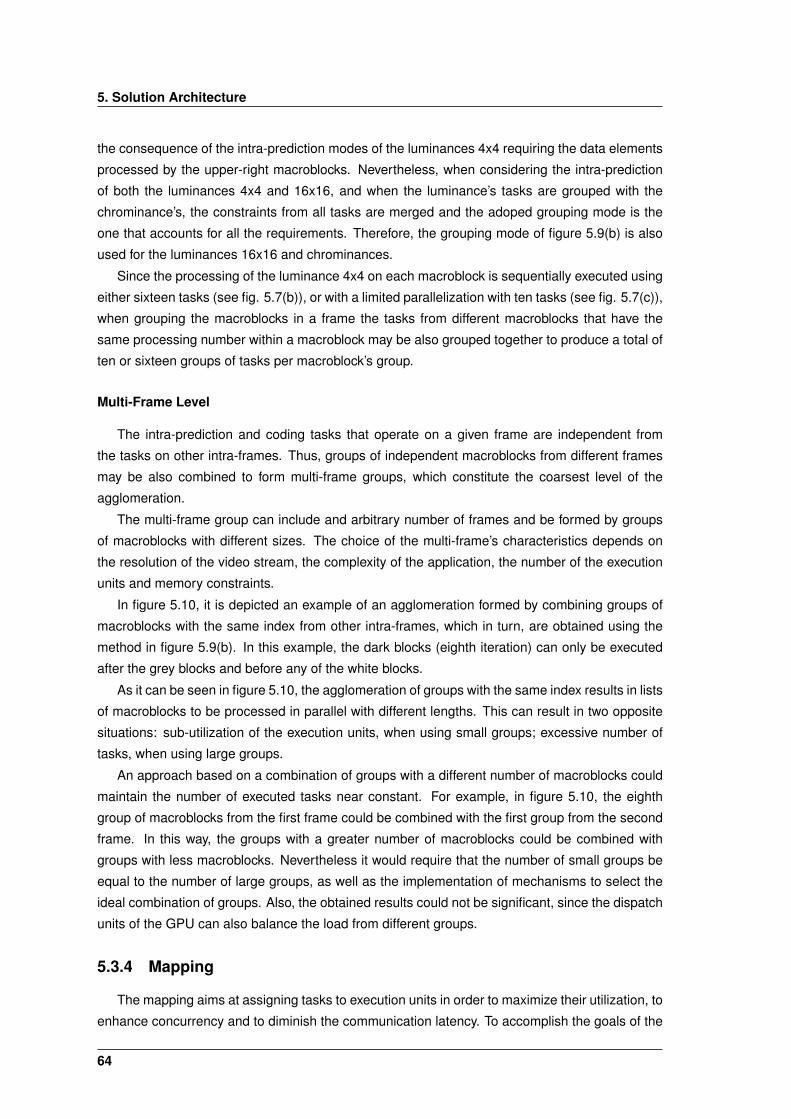
5. Solution Architecture
the consequence of the intra-prediction modes of the luminances 4x4 requiring the data elements
processed by the upper-right macroblocks. Nevertheless, when considering the intra-prediction
of both the luminances 4x4 and 16x16, and when the luminance’s tasks are grouped with the
chrominance’s, the constraints from all tasks are merged and the adoped grouping mode is the
one that accounts for all the requirements. Therefore, the grouping mode of figure 5.9(b) is also
used for the luminances 16x16 and chrominances.
Since the processing of the luminance 4x4 on each macroblock is sequentially executed using
either sixteen tasks (see fig. 5.7(b)), or with a limited parallelization with ten tasks (see fig. 5.7(c)),
when grouping the macroblocks in a frame the tasks from different macroblocks that have the
same processing number within a macroblock may be also grouped together to produce a total of
ten or sixteen groups of tasks per macroblock’s group.
Multi-Frame Level
The intra-prediction and coding tasks that operate on a given frame are independent from
the tasks on other intra-frames. Thus, groups of independent macroblocks from different frames
may be also combined to form multi-frame groups, which constitute the coarsest level of the
agglomeration.
The multi-frame group can include and arbitrary number of frames and be formed by groups
of macroblocks with different sizes. The choice of the multi-frame’s characteristics depends on
the resolution of the video stream, the complexity of the application, the number of the execution
units and memory constraints.
In figure 5.10, it is depicted an example of an agglomeration formed by combining groups of
macroblocks with the same index from other intra-frames, which in turn, are obtained using the
method in figure 5.9(b). In this example, the dark blocks (eighth iteration) can only be executed
after the grey blocks and before any of the white blocks.
As it can be seen in figure 5.10, the agglomeration of groups with the same index results in lists
of macroblocks to be processed in parallel with different lengths. This can result in two opposite
situations: sub-utilization of the execution units, when using small groups; excessive number of
tasks, when using large groups.
An approach based on a combination of groups with a different number of macroblocks could
maintain the number of executed tasks near constant. For example, in figure 5.10, the eighth
group of macroblocks from the first frame could be combined with the first group from the second
frame. In this way, the groups with a greater number of macroblocks could be combined with
groups with less macroblocks. Nevertheless it would require that the number of small groups be
equal to the number of large groups, as well as the implementation of mechanisms to select the
ideal combination of groups. Also, the obtained results could not be significant, since the dispatch
units of the GPU can also balance the load from different groups.
5.3.4 Mapping
The mapping aims at assigning tasks to execution units in order to maximize their utilization, to
enhance concurrency and to diminish the communication latency. To accomplish the goals of the
64
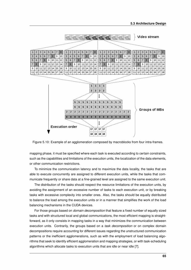
5.3 Architecture Design
Figure 5.10: Example of an agglomeration composed by macroblocks from four intra-frames.
mapping phase, it must be specified where each task is executed according to certain constraints,
such as the capabilities and limitations of the execution units, the localization of the data elements,
or other communication restrictions.
To minimize the communication latency and to maximize the data locality, the tasks that are
able to execute concurrently are assigned to different execution units, while the tasks that com-
municate frequently or share data at a fine-grained level are assigned to the same execution unit.
The distribution of the tasks should respect the resource limitations of the execution units, by
avoiding the assignment of an excessive number of tasks to each execution unit, or by breaking
tasks with excessive complexity into smaller ones. Also, the tasks should be equally distributed
to balance the load among the execution units or in a manner that simplifies the work of the load
balancing mechanisms in the CUDA devices.
For those groups based on domain decomposition that feature a fixed number of equally sized
tasks and with structured local and global communications, the most efficient mapping is straight-
forward, as it only consists in mapping tasks in a way that minimizes the communication between
execution units. Contrarily, the groups based on a task decomposition or on complex domain
decompositions require accounting for different issues regarding the unstructured communication
patterns or the inefficient agglomerations, such as with the employment of load balancing algo-
rithms that seek to identify efficient agglomeration and mapping strategies, or with task-scheduling
algorithms which allocate tasks to execution units that are idle or near idle [7].
65
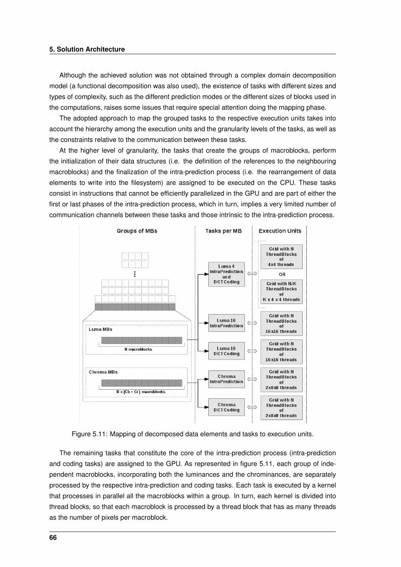
5. Solution Architecture
Although the achieved solution was not obtained through a complex domain decomposition
model (a functional decomposition was also used), the existence of tasks with different sizes and
types of complexity, such as the different prediction modes or the different sizes of blocks used in
the computations, raises some issues that require special attention doing the mapping phase.
The adopted approach to map the grouped tasks to the respective execution units takes into
account the hierarchy among the execution units and the granularity levels of the tasks, as well as
the constraints relative to the communication between these tasks.
At the higher level of granularity, the tasks that create the groups of macroblocks, perform
the initialization of their data structures (i.e. the definition of the references to the neighbouring
macroblocks) and the finalization of the intra-prediction process (i.e. the rearrangement of data
elements to write into the filesystem) are assigned to be executed on the CPU. These tasks
consist in instructions that cannot be efficiently parallelized in the GPU and are part of either the
first or last phases of the intra-prediction process, which in turn, implies a very limited number of
communication channels between these tasks and those intrinsic to the intra-prediction process.
Figure 5.11: Mapping of decomposed data elements and tasks to execution units.
The remaining tasks that constitute the core of the intra-prediction process (intra-prediction
and coding tasks) are assigned to the GPU. As represented in figure 5.11, each group of inde-
pendent macroblocks, incorporating both the luminances and the chrominances, are separately
processed by the respective intra-prediction and coding tasks. Each task is executed by a kernel
that processes in parallel all the macroblocks within a group. In turn, each kernel is divided into
thread blocks, so that each macroblock is processed by a thread block that has as many threads
as the number of pixels per macroblock.
66
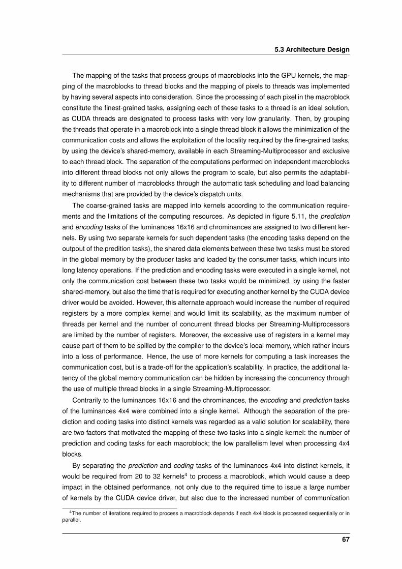
5.3 Architecture Design
The mapping of the tasks that process groups of macroblocks into the GPU kernels, the map-
ping of the macroblocks to thread blocks and the mapping of pixels to threads was implemented
by having several aspects into consideration. Since the processing of each pixel in the macroblock
constitute the finest-grained tasks, assigning each of these tasks to a thread is an ideal solution,
as CUDA threads are designated to process tasks with very low granularity. Then, by grouping
the threads that operate in a macroblock into a single thread block it allows the minimization of the
communication costs and allows the exploitation of the locality required by the fine-grained tasks,
by using the device’s shared-memory, available in each Streaming-Multiprocessor and exclusive
to each thread block. The separation of the computations performed on independent macroblocks
into different thread blocks not only allows the program to scale, but also permits the adaptabil-
ity to different number of macroblocks through the automatic task scheduling and load balancing
mechanisms that are provided by the device’s dispatch units.
The coarse-grained tasks are mapped into kernels according to the communication require-
ments and the limitations of the computing resources. As depicted in figure 5.11, the prediction
and encoding tasks of the luminances 16x16 and chrominances are assigned to two different ker-
nels. By using two separate kernels for such dependent tasks (the encoding tasks depend on the
outpout of the predition tasks), the shared data elements between these two tasks must be stored
in the global memory by the producer tasks and loaded by the consumer tasks, which incurs into
long latency operations. If the prediction and encoding tasks were executed in a single kernel, not
only the communication cost between these two tasks would be minimized, by using the faster
shared-memory, but also the time that is required for executing another kernel by the CUDA device
driver would be avoided. However, this alternate approach would increase the number of required
registers by a more complex kernel and would limit its scalability, as the maximum number of
threads per kernel and the number of concurrent thread blocks per Streaming-Multiprocessors
are limited by the number of registers. Moreover, the excessive use of registers in a kernel may
cause part of them to be spilled by the compiler to the device’s local memory, which rather incurs
into a loss of performance. Hence, the use of more kernels for computing a task increases the
communication cost, but is a trade-off for the application’s scalability. In practice, the additional la-
tency of the global memory communication can be hidden by increasing the concurrency through
the use of multiple thread blocks in a single Streaming-Multiprocessor.
Contrarily to the luminances 16x16 and the chrominances, the encoding and prediction tasks
of the luminances 4x4 were combined into a single kernel. Although the separation of the pre-
diction and coding tasks into distinct kernels was regarded as a valid solution for scalability, there
are two factors that motivated the mapping of these two tasks into a single kernel: the number of
prediction and coding tasks for each macroblock; the low parallelism level when processing 4x4
blocks.
By separating the prediction and coding tasks of the luminances 4x4 into distinct kernels, it
would be required from 20 to 32 kernels4 to process a macroblock, which would cause a deep
impact in the obtained performance, not only due to the required time to issue a large number
of kernels by the CUDA device driver, but also due to the increased number of communication
4The number of iterations required to process a macroblock depends if each 4x4 block is processed sequentially or inparallel.
67
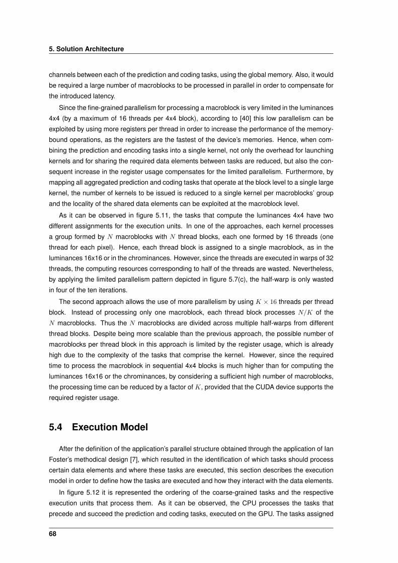
5. Solution Architecture
channels between each of the prediction and coding tasks, using the global memory. Also, it would
be required a large number of macroblocks to be processed in parallel in order to compensate for
the introduced latency.
Since the fine-grained parallelism for processing a macroblock is very limited in the luminances
4x4 (by a maximum of 16 threads per 4x4 block), according to [40] this low parallelism can be
exploited by using more registers per thread in order to increase the performance of the memory-
bound operations, as the registers are the fastest of the device’s memories. Hence, when com-
bining the prediction and encoding tasks into a single kernel, not only the overhead for launching
kernels and for sharing the required data elements between tasks are reduced, but also the con-
sequent increase in the register usage compensates for the limited parallelism. Furthermore, by
mapping all aggregated prediction and coding tasks that operate at the block level to a single large
kernel, the number of kernels to be issued is reduced to a single kernel per macroblocks’ group
and the locality of the shared data elements can be exploited at the macroblock level.
As it can be observed in figure 5.11, the tasks that compute the luminances 4x4 have two
different assignments for the execution units. In one of the approaches, each kernel processes
a group formed by N macroblocks with N thread blocks, each one formed by 16 threads (one
thread for each pixel). Hence, each thread block is assigned to a single macroblock, as in the
luminances 16x16 or in the chrominances. However, since the threads are executed in warps of 32
threads, the computing resources corresponding to half of the threads are wasted. Nevertheless,
by applying the limited parallelism pattern depicted in figure 5.7(c), the half-warp is only wasted
in four of the ten iterations.
The second approach allows the use of more parallelism by using K × 16 threads per thread
block. Instead of processing only one macroblock, each thread block processes N/K of the
N macroblocks. Thus the N macroblocks are divided across multiple half-warps from different
thread blocks. Despite being more scalable than the previous approach, the possible number of
macroblocks per thread block in this approach is limited by the register usage, which is already
high due to the complexity of the tasks that comprise the kernel. However, since the required
time to process the macroblock in sequential 4x4 blocks is much higher than for computing the
luminances 16x16 or the chrominances, by considering a sufficient high number of macroblocks,
the processing time can be reduced by a factor of K, provided that the CUDA device supports the
required register usage.
5.4 Execution Model
After the definition of the application’s parallel structure obtained through the application of Ian
Foster’s methodical design [7], which resulted in the identification of which tasks should process
certain data elements and where these tasks are executed, this section describes the execution
model in order to define how the tasks are executed and how they interact with the data elements.
In figure 5.12 it is represented the ordering of the coarse-grained tasks and the respective
execution units that process them. As it can be observed, the CPU processes the tasks that
precede and succeed the prediction and coding tasks, executed on the GPU. The tasks assigned
68
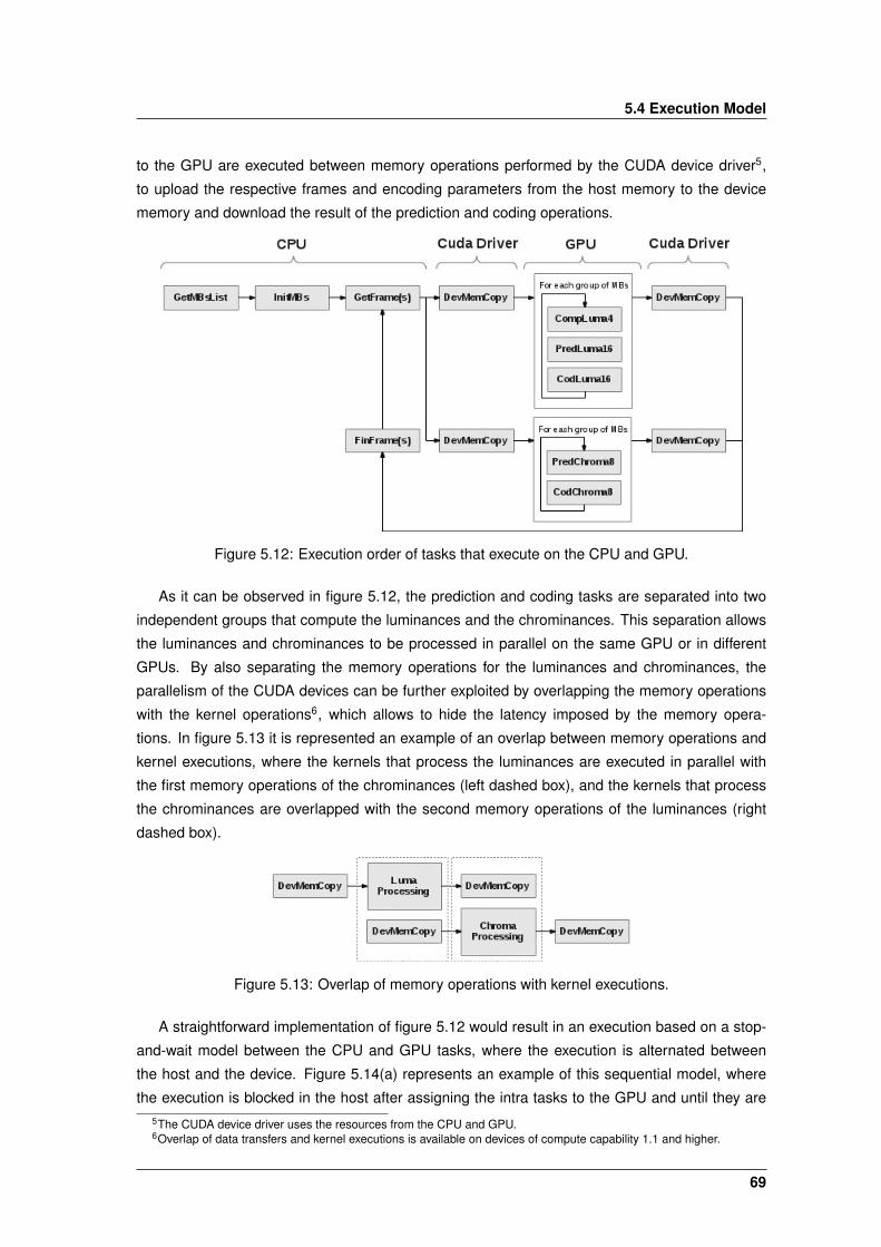
5.4 Execution Model
to the GPU are executed between memory operations performed by the CUDA device driver5,
to upload the respective frames and encoding parameters from the host memory to the device
memory and download the result of the prediction and coding operations.
Figure 5.12: Execution order of tasks that execute on the CPU and GPU.
As it can be observed in figure 5.12, the prediction and coding tasks are separated into two
independent groups that compute the luminances and the chrominances. This separation allows
the luminances and chrominances to be processed in parallel on the same GPU or in different
GPUs. By also separating the memory operations for the luminances and chrominances, the
parallelism of the CUDA devices can be further exploited by overlapping the memory operations
with the kernel operations6, which allows to hide the latency imposed by the memory opera-
tions. In figure 5.13 it is represented an example of an overlap between memory operations and
kernel executions, where the kernels that process the luminances are executed in parallel with
the first memory operations of the chrominances (left dashed box), and the kernels that process
the chrominances are overlapped with the second memory operations of the luminances (right
dashed box).
Figure 5.13: Overlap of memory operations with kernel executions.
A straightforward implementation of figure 5.12 would result in an execution based on a stop-
and-wait model between the CPU and GPU tasks, where the execution is alternated between
the host and the device. Figure 5.14(a) represents an example of this sequential model, where
the execution is blocked in the host after assigning the intra tasks to the GPU and until they are5The CUDA device driver uses the resources from the CPU and GPU.6Overlap of data transfers and kernel executions is available on devices of compute capability 1.1 and higher.
69
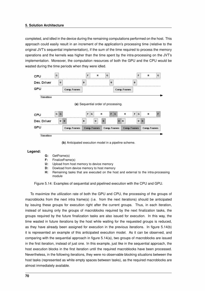
5. Solution Architecture
completed, and idled in the device during the remaining computations performed on the host. This
approach could easily result in an increment of the application’s processing time (relative to the
original JVT’s sequential implementation), if the sum of the time required to process the memory
operations and the kernels was higher than the time spent by the intra-processing on the JVT’s
implementation. Moreover, the computation resources of both the GPU and the CPU would be
wasted during the time periods when they were idled.
(a) Sequential order of processing.
(b) Anticipated execution model in a pipeline scheme.
Legend:G: GetFrame(s)F: FinalizeFrame(s)U: Upload from host memory to device memoryD: Dowload from device memory to host memoryH: Remaining tasks that are executed on the host and external to the intra-processing
module
Figure 5.14: Examples of sequential and pipelined execution with the CPU and GPU.
To maximize the utilization rate of both the GPU and CPU, the processing of the groups of
macroblocks from the next intra frame(s) (i.e. from the next iterations) should be anticipated
by issuing these groups for execution right after the current groups. Thus, in each iteration,
instead of issuing only the groups of macroblocks required by the next finalization tasks, the
groups required by the future finalization tasks are also issued for execution. In this way, the
time wasted in future iterations by the host while waiting for the requested groups is reduced,
as they have already been assigned for execution in the previous iterations. In figure 5.14(b)
it is represented an example of this anticipated execution model. As it can be observed, and
comparing with the sequential approach in figure 5.14(a), two groups of macroblocks are issued
in the first iteration, instead of just one. In this example, just like in the sequential approach, the
host execution blocks in the first iteration until the required macroblocks have been processed.
Nevertheless, in the following iterations, they were no observable blocking situations between the
host tasks (represented as white empty spaces between tasks), as the required macroblocks are
almost immediately available.
70
5.4 Execution Model
To permit this anticipatory execution of the prediction and coding tasks, all the tasks that
are executed on the device or through the device driver must be asynchronously issued from
the host. These asynchronous operations must respect the order of dependent tasks and must
use synchronization points before the respective finalization tasks. As it can be observed in
figure 5.14(b), the asynchronous execution also permits both the overlapping between the tasks
assigned to compute the frames and the memory operations from other tasks and the execution
of concurrent or parallel kernels7.
The coarse-grained implementation of the intra-prediction process, according to the anticipa-
tory execution model depicted in figure 5.14(b) and represented in algorithm 5.5, which represents
the operations performed in the host (including those that assign the execution to the device). It
also represents a parallel version of the sequential algorithm 5.1.
In algorithm 5.5, the concurrency of several lists of macroblocks is implemented by using
several queues, where each queue corresponds to a list with groups of macroblocks that belongs
to one or more consecutive intra-frames. The execution starts by asynchronously issuing the
prediction and coding tasks of all macroblocks from each empty queue to the device (see line
3). When the device tasks from all queues have been assigned, the host execution blocks until
the queue that contains the current frame completes (see line 7). The required frame for the
finalization process (see line 15) is retrieved from the queue in line 9.
Algorithm 5.5 Parallel Macroblock Intra-Prediction per Frame.
1: for each queue in total queues do2: if empty queue(queue) then3: process queue(queue)4: end if5: end for6: if not ready(current queue) then7: wait(current queue)8: end if9: dequeue(current queue)→ encoded data
10: if empty(current queue) then11: process queue(current queue) # The same instructions as in the previous process queue12: switch queues(current queue)13: end if14: for each macroblock in frame macroblocks do15: finish macroblock(macroblock)16: end for
For each one of the previous queues there is one queue in the host’s memory to store the
computed frames. The data elements regarding the process of a current frame are then retrieved
from one of this queues to be processed by the finalization tasks (see line 9). After all its frames
have been processed, the hosts’s queues are swapped (see line 12) in order to allow the empty
queue to store the next frames to be processed while the future finalization tasks process the data
elements from other queues.
The assignment of each queue containing lists of macroblocks to the GPU is depicted in lines
3 and 11. The second assignment (in line 11) is required to immediately issue a recently emptied
7The more recent CUDA devices support a limited number of parallel kernels.
71
5. Solution Architecture
queue to execution in order to maximize the number of concurrent queues. Each of these two
operations is detailed in algorithm 5.6, which consists in the host’s operations to fetch the intra-
frames from the filesystem (see line 1), in the device’s operations to upload the frames (see lines 2
and 4, the process of the intra-prediction and coding tasks (see lines 3 and 5), and the procedures
to download the encoded data elements from the device’s memory (see lines 6 and 7).
The possibility of using a different number of queues and a different number of frames per
queue not only permits the adaptability to CUDA devices with different characteristics, but also
the use of multiple CUDA devices.
Algorithm 5.6 Intra-Process.
1: get frames(num frames)→ luma frame, cb frame, cr frame2: upload luma(luma frame)3: process luma()4: upload chroma(cb frame, cr frame)5: process chroma()6: download luma()→ enc luma7: download chroma()→ enc cb, enc cr
72
6Implementation Process
Contents6.1 Implemented Data Structures . . . . . . . . . . . . . . . . . . . . . . . . . . . . 746.2 Asynchronous Execution Model . . . . . . . . . . . . . . . . . . . . . . . . . . . 756.3 Optimizations . . . . . . . . . . . . . . . . . . . . . . . . . . . . . . . . . . . . . 75
73
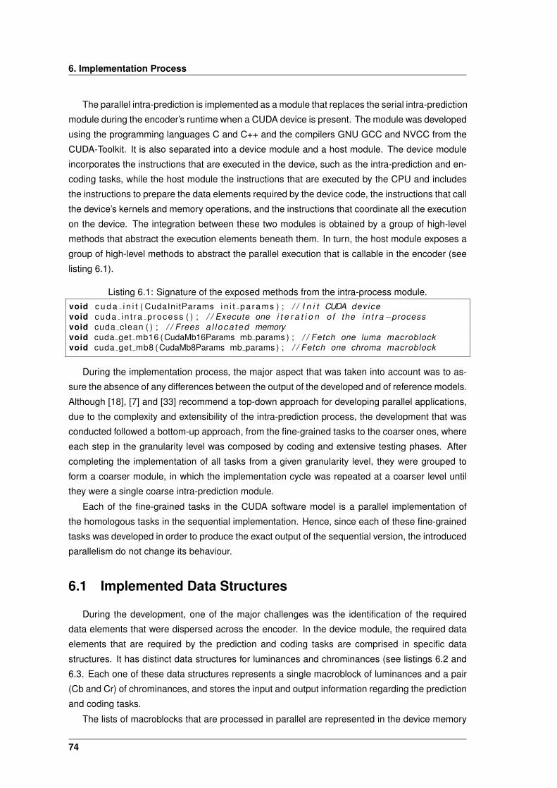
6. Implementation Process
The parallel intra-prediction is implemented as a module that replaces the serial intra-prediction
module during the encoder’s runtime when a CUDA device is present. The module was developed
using the programming languages C and C++ and the compilers GNU GCC and NVCC from the
CUDA-Toolkit. It is also separated into a device module and a host module. The device module
incorporates the instructions that are executed in the device, such as the intra-prediction and en-
coding tasks, while the host module the instructions that are executed by the CPU and includes
the instructions to prepare the data elements required by the device code, the instructions that call
the device’s kernels and memory operations, and the instructions that coordinate all the execution
on the device. The integration between these two modules is obtained by a group of high-level
methods that abstract the execution elements beneath them. In turn, the host module exposes a
group of high-level methods to abstract the parallel execution that is callable in the encoder (see
listing 6.1).
Listing 6.1: Signature of the exposed methods from the intra-process module.void c u d a i n i t ( CudaInitParams in i t pa rams ) ; / / I n i t CUDA devicevoid cuda in t ra p rocess ( ) ; / / Execute one i t e r a t i o n o f the i n t r a−processvoid cuda clean ( ) ; / / Frees a l l oc a t e d memoryvoid cuda get mb16 (CudaMb16Params mb params ) ; / / Fetch one luma macroblockvoid cuda get mb8 (CudaMb8Params mb params ) ; / / Fetch one chroma macroblock
During the implementation process, the major aspect that was taken into account was to as-
sure the absence of any differences between the output of the developed and of reference models.
Although [18], [7] and [33] recommend a top-down approach for developing parallel applications,
due to the complexity and extensibility of the intra-prediction process, the development that was
conducted followed a bottom-up approach, from the fine-grained tasks to the coarser ones, where
each step in the granularity level was composed by coding and extensive testing phases. After
completing the implementation of all tasks from a given granularity level, they were grouped to
form a coarser module, in which the implementation cycle was repeated at a coarser level until
they were a single coarse intra-prediction module.
Each of the fine-grained tasks in the CUDA software model is a parallel implementation of
the homologous tasks in the sequential implementation. Hence, since each of these fine-grained
tasks was developed in order to produce the exact output of the sequential version, the introduced
parallelism do not change its behaviour.
6.1 Implemented Data Structures
During the development, one of the major challenges was the identification of the required
data elements that were dispersed across the encoder. In the device module, the required data
elements that are required by the prediction and coding tasks are comprised in specific data
structures. It has distinct data structures for luminances and chrominances (see listings 6.2 and
6.3. Each one of these data structures represents a single macroblock of luminances and a pair
(Cb and Cr) of chrominances, and stores the input and output information regarding the prediction
and coding tasks.
The lists of macroblocks that are processed in parallel are represented in the device memory
74
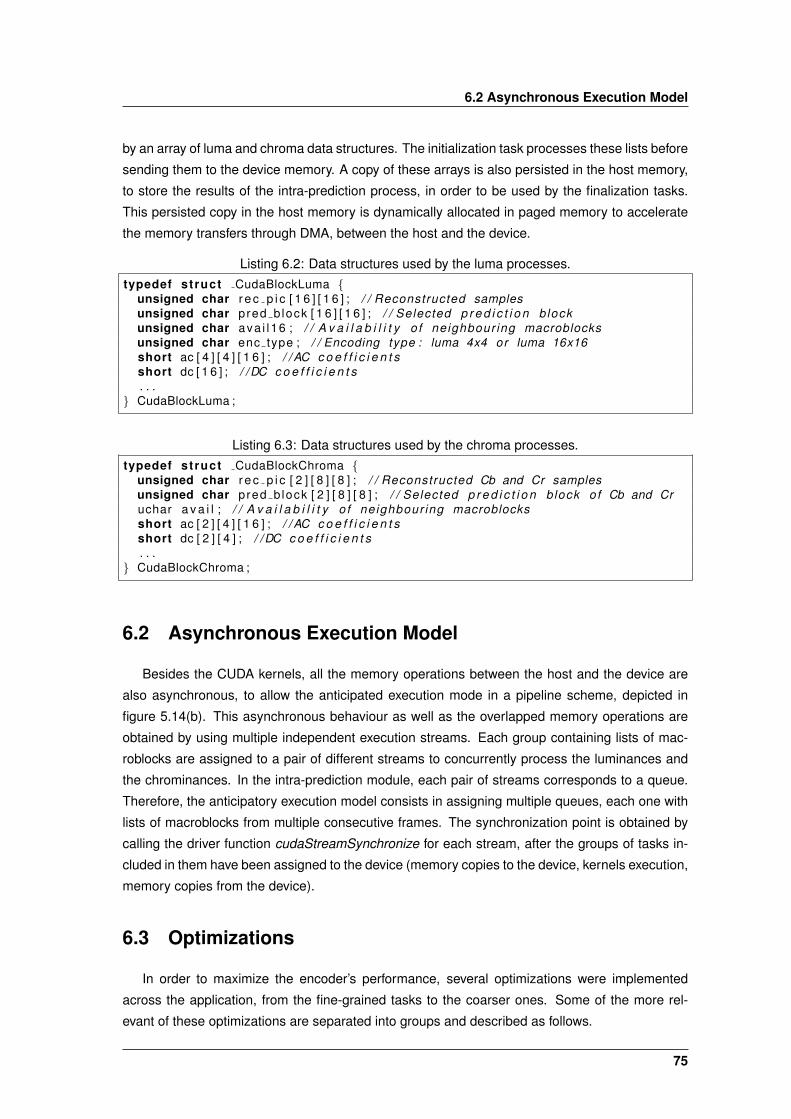
6.2 Asynchronous Execution Model
by an array of luma and chroma data structures. The initialization task processes these lists before
sending them to the device memory. A copy of these arrays is also persisted in the host memory,
to store the results of the intra-prediction process, in order to be used by the finalization tasks.
This persisted copy in the host memory is dynamically allocated in paged memory to accelerate
the memory transfers through DMA, between the host and the device.
Listing 6.2: Data structures used by the luma processes.typedef struct CudaBlockLuma {
unsigned char r e c p i c [ 1 6 ] [ 1 6 ] ; / / Reconstructed samplesunsigned char pred b lock [ 1 6 ] [ 1 6 ] ; / / Selected p r e d i c t i o n blockunsigned char ava i l 16 ; / / A v a i l a b i l i t y o f neighbour ing macroblocksunsigned char enc type ; / / Encoding type : luma 4x4 or luma 16x16short ac [ 4 ] [ 4 ] [ 1 6 ] ; / / AC c o e f f i c i e n t sshort dc [ 1 6 ] ; / /DC c o e f f i c i e n t s. . .
} CudaBlockLuma ;
Listing 6.3: Data structures used by the chroma processes.typedef struct CudaBlockChroma {
unsigned char r e c p i c [ 2 ] [ 8 ] [ 8 ] ; / / Reconstructed Cb and Cr samplesunsigned char pred b lock [ 2 ] [ 8 ] [ 8 ] ; / / Selected p r e d i c t i o n block o f Cb and Cruchar a v a i l ; / / A v a i l a b i l i t y o f neighbour ing macroblocksshort ac [ 2 ] [ 4 ] [ 1 6 ] ; / / AC c o e f f i c i e n t sshort dc [ 2 ] [ 4 ] ; / /DC c o e f f i c i e n t s. . .
} CudaBlockChroma ;
6.2 Asynchronous Execution Model
Besides the CUDA kernels, all the memory operations between the host and the device are
also asynchronous, to allow the anticipated execution mode in a pipeline scheme, depicted in
figure 5.14(b). This asynchronous behaviour as well as the overlapped memory operations are
obtained by using multiple independent execution streams. Each group containing lists of mac-
roblocks are assigned to a pair of different streams to concurrently process the luminances and
the chrominances. In the intra-prediction module, each pair of streams corresponds to a queue.
Therefore, the anticipatory execution model consists in assigning multiple queues, each one with
lists of macroblocks from multiple consecutive frames. The synchronization point is obtained by
calling the driver function cudaStreamSynchronize for each stream, after the groups of tasks in-
cluded in them have been assigned to the device (memory copies to the device, kernels execution,
memory copies from the device).
6.3 Optimizations
In order to maximize the encoder’s performance, several optimizations were implemented
across the application, from the fine-grained tasks to the coarser ones. Some of the more rel-
evant of these optimizations are separated into groups and described as follows.
75
6. Implementation Process
Coalesced Memory Access
One of the major concerns regarding the performance of a running kernel is the memory
access patterns that can degrade the performance with more than one order of magnitude. Hence,
several techniques were taken into account for the memory accesses.
One of these techniques is related to the alignment of the declared data structures to avoid
uncoalesced patterns and reduce the number of cache misses when accessing its elements.
Since the declaration using the function cudaMalloc guarantees an alignment of at least 256
bytes [6], the data elements allocated in the device global memory are organized to exploit this
alignment, by using the align (n) alignment specifier, which forces the nvidia compiler to align
the elements in a structure of n bytes.
When using groups of multiple elements, such as the structures in listings 6.2 and 6.3, they
are organized into Structures of Arrays (SoA) instead of Arrays of Structures (AoS), to avoid
coalescing issues [6] when aligning each of these arrays. Since each structure is associated
to a macroblock and consequently to a thread block, the way in which multiple structures are
organized does not influence the coalesced access, as long as the organization of their elements
is suitable for coalesced accesses. Therefore, the lists of macroblocks are organized in arrays
of SoA, where all the lists that are used in the same execution stream are allocated in the same
array. This single array facilitates the access of the reconstructed samples from the prediction
tasks to the neighbouring macroblocks.
Memory Compression
While the organization of data elements using SoA is more suitable for parallel access pat-
terns, the organization of data elements using AoS is more suitable for broadcast accesses (i.e.
multiple threads accessing the same memory location). Hence, the data elements that are ac-
cessed by broadcast are compressed into a single structure with the maximum size of a cache
line, in order to reduce the access of all its elements into a single memory access.
Memory Prefetching
Recent CUDA devices support the prefetch of memory elements. With this feature, some
assignment operations can be anticipated in a few lines of the source-code allowing the execution
to continue until the requested value has been required by some instruction. This feature is
possible due to the existence of independent Load/Store units and execution cores that allow the
simultaneous execution of computing instructions with memory fetch operations (see fig. 3.7).
This approach permits the reduction of the latency imposed by the memory operations and can
compensate for the in-order execution of the CUDA processors, by manually assigning the order
of the executed instructions. Nevertheless, this prefetch of assignment operations not only may
incur in an increase on the register usage, but also the obtained results may vary across different
CUDA devices. Moreover, to efficiently implement the prefetching, the distance (in instruction
cycles) between a memory assignment operation and the respective use of the assigned value
must be at least equal to the latency of the memory operation.
76
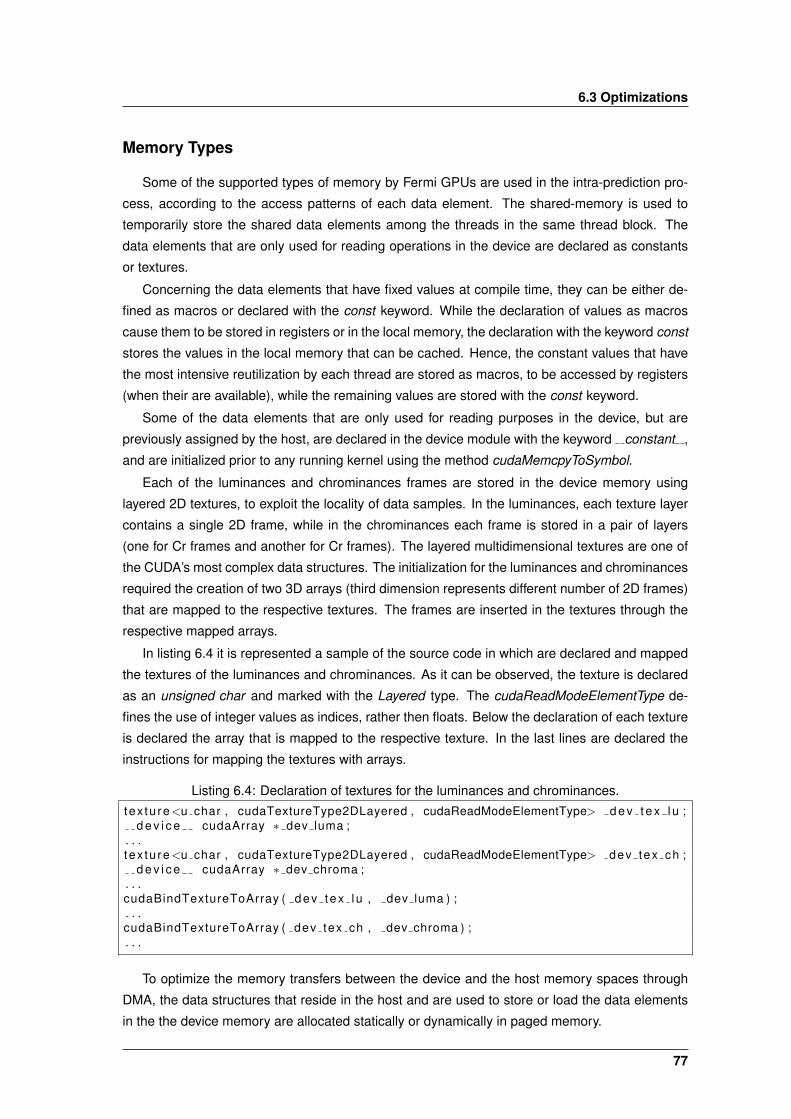
6.3 Optimizations
Memory Types
Some of the supported types of memory by Fermi GPUs are used in the intra-prediction pro-
cess, according to the access patterns of each data element. The shared-memory is used to
temporarily store the shared data elements among the threads in the same thread block. The
data elements that are only used for reading operations in the device are declared as constants
or textures.
Concerning the data elements that have fixed values at compile time, they can be either de-
fined as macros or declared with the const keyword. While the declaration of values as macros
cause them to be stored in registers or in the local memory, the declaration with the keyword const
stores the values in the local memory that can be cached. Hence, the constant values that have
the most intensive reutilization by each thread are stored as macros, to be accessed by registers
(when their are available), while the remaining values are stored with the const keyword.
Some of the data elements that are only used for reading purposes in the device, but are
previously assigned by the host, are declared in the device module with the keyword constant ,
and are initialized prior to any running kernel using the method cudaMemcpyToSymbol.
Each of the luminances and chrominances frames are stored in the device memory using
layered 2D textures, to exploit the locality of data samples. In the luminances, each texture layer
contains a single 2D frame, while in the chrominances each frame is stored in a pair of layers
(one for Cr frames and another for Cr frames). The layered multidimensional textures are one of
the CUDA’s most complex data structures. The initialization for the luminances and chrominances
required the creation of two 3D arrays (third dimension represents different number of 2D frames)
that are mapped to the respective textures. The frames are inserted in the textures through the
respective mapped arrays.
In listing 6.4 it is represented a sample of the source code in which are declared and mapped
the textures of the luminances and chrominances. As it can be observed, the texture is declared
as an unsigned char and marked with the Layered type. The cudaReadModeElementType de-
fines the use of integer values as indices, rather then floats. Below the declaration of each texture
is declared the array that is mapped to the respective texture. In the last lines are declared the
instructions for mapping the textures with arrays.
Listing 6.4: Declaration of textures for the luminances and chrominances.t ex tu re<u char , cudaTextureType2DLayered , cudaReadModeElementType> d e v t e x l u ;
d e v i c e cudaArray ∗ dev luma ;. . .t ex tu re<u char , cudaTextureType2DLayered , cudaReadModeElementType> dev tex ch ;
d e v i c e cudaArray ∗ dev chroma ;. . .cudaBindTextureToArray ( dev tex l u , dev luma ) ;. . .cudaBindTextureToArray ( dev tex ch , dev chroma ) ;. . .
To optimize the memory transfers between the device and the host memory spaces through
DMA, the data structures that reside in the host and are used to store or load the data elements
in the the device memory are allocated statically or dynamically in paged memory.
77
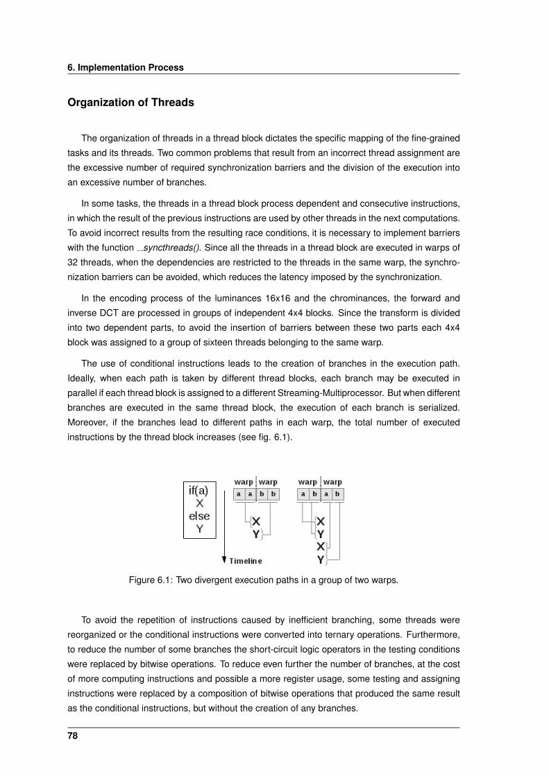
6. Implementation Process
Organization of Threads
The organization of threads in a thread block dictates the specific mapping of the fine-grained
tasks and its threads. Two common problems that result from an incorrect thread assignment are
the excessive number of required synchronization barriers and the division of the execution into
an excessive number of branches.
In some tasks, the threads in a thread block process dependent and consecutive instructions,
in which the result of the previous instructions are used by other threads in the next computations.
To avoid incorrect results from the resulting race conditions, it is necessary to implement barriers
with the function syncthreads(). Since all the threads in a thread block are executed in warps of
32 threads, when the dependencies are restricted to the threads in the same warp, the synchro-
nization barriers can be avoided, which reduces the latency imposed by the synchronization.
In the encoding process of the luminances 16x16 and the chrominances, the forward and
inverse DCT are processed in groups of independent 4x4 blocks. Since the transform is divided
into two dependent parts, to avoid the insertion of barriers between these two parts each 4x4
block was assigned to a group of sixteen threads belonging to the same warp.
The use of conditional instructions leads to the creation of branches in the execution path.
Ideally, when each path is taken by different thread blocks, each branch may be executed in
parallel if each thread block is assigned to a different Streaming-Multiprocessor. But when different
branches are executed in the same thread block, the execution of each branch is serialized.
Moreover, if the branches lead to different paths in each warp, the total number of executed
instructions by the thread block increases (see fig. 6.1).
Figure 6.1: Two divergent execution paths in a group of two warps.
To avoid the repetition of instructions caused by inefficient branching, some threads were
reorganized or the conditional instructions were converted into ternary operations. Furthermore,
to reduce the number of some branches the short-circuit logic operators in the testing conditions
were replaced by bitwise operations. To reduce even further the number of branches, at the cost
of more computing instructions and possible a more register usage, some testing and assigning
instructions were replaced by a composition of bitwise operations that produced the same result
as the conditional instructions, but without the creation of any branches.
78
6.3 Optimizations
Optimization in Computations
Because the CUDA devices have a large discrepancy between the latency of the memory
operations and the arithmetic computations, during the execution path of some instructions and
when is required to save some registers, some required values are recalculated instead of storing
the previous results in long latency memories. Also, some instructions are separated into inde-
pendent computations and grouped in the source-code to exploit the available Instruction-Level
Parallelism (ILP) [40].
Moreover, when implementing in parallel some tasks that were optimized for sequential exe-
cution, some light-weight computations were converted into heavier computations to exploit the
parallelism, where the parallelism of slow tasks compensate for faster sequential execution. One
example is the sequential implementation of the DCT, that is essentially composed by depen-
dent groups of shift and adding operations, but the dependency of these operations restrict the
parallelism to only four threads when processing 4x4 blocks. By replacing these light-weigh shift
and addition operations by heavier multiplication operations, the DCT could be parallelized with
sixteen threads and with an increase of 25% in the resulting performance.
79

6. Implementation Process
80

7Results
Contents7.1 Performance Characterization . . . . . . . . . . . . . . . . . . . . . . . . . . . . 827.2 Testing Hardware . . . . . . . . . . . . . . . . . . . . . . . . . . . . . . . . . . . 827.3 Performance . . . . . . . . . . . . . . . . . . . . . . . . . . . . . . . . . . . . . . 837.4 Analysis of Scalability . . . . . . . . . . . . . . . . . . . . . . . . . . . . . . . . 897.5 Discussion . . . . . . . . . . . . . . . . . . . . . . . . . . . . . . . . . . . . . . . 90
81
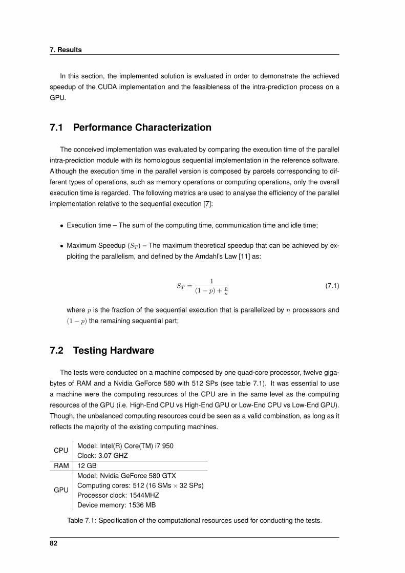
7. Results
In this section, the implemented solution is evaluated in order to demonstrate the achieved
speedup of the CUDA implementation and the feasibleness of the intra-prediction process on a
GPU.
7.1 Performance Characterization
The conceived implementation was evaluated by comparing the execution time of the parallel
intra-prediction module with its homologous sequential implementation in the reference software.
Although the execution time in the parallel version is composed by parcels corresponding to dif-
ferent types of operations, such as memory operations or computing operations, only the overall
execution time is regarded. The following metrics are used to analyse the efficiency of the parallel
implementation relative to the sequential execution [7]:
• Execution time – The sum of the computing time, communication time and idle time;
• Maximum Speedup (ST ) – The maximum theoretical speedup that can be achieved by ex-
ploiting the parallelism, and defined by the Amdahl’s Law [11] as:
ST =1
(1− p) + pn
(7.1)
where p is the fraction of the sequential execution that is parallelized by n processors and
(1− p) the remaining sequential part;
7.2 Testing Hardware
The tests were conducted on a machine composed by one quad-core processor, twelve giga-
bytes of RAM and a Nvidia GeForce 580 with 512 SPs (see table 7.1). It was essential to use
a machine were the computing resources of the CPU are in the same level as the computing
resources of the GPU (i.e. High-End CPU vs High-End GPU or Low-End CPU vs Low-End GPU).
Though, the unbalanced computing resources could be seen as a valid combination, as long as it
reflects the majority of the existing computing machines.
CPUModel: Intel(R) Core(TM) i7 950Clock: 3.07 GHZ
RAM 12 GB
GPU
Model: Nvidia GeForce 580 GTXComputing cores: 512 (16 SMs× 32 SPs)Processor clock: 1544MHZDevice memory: 1536 MB
Table 7.1: Specification of the computational resources used for conducting the tests.
82
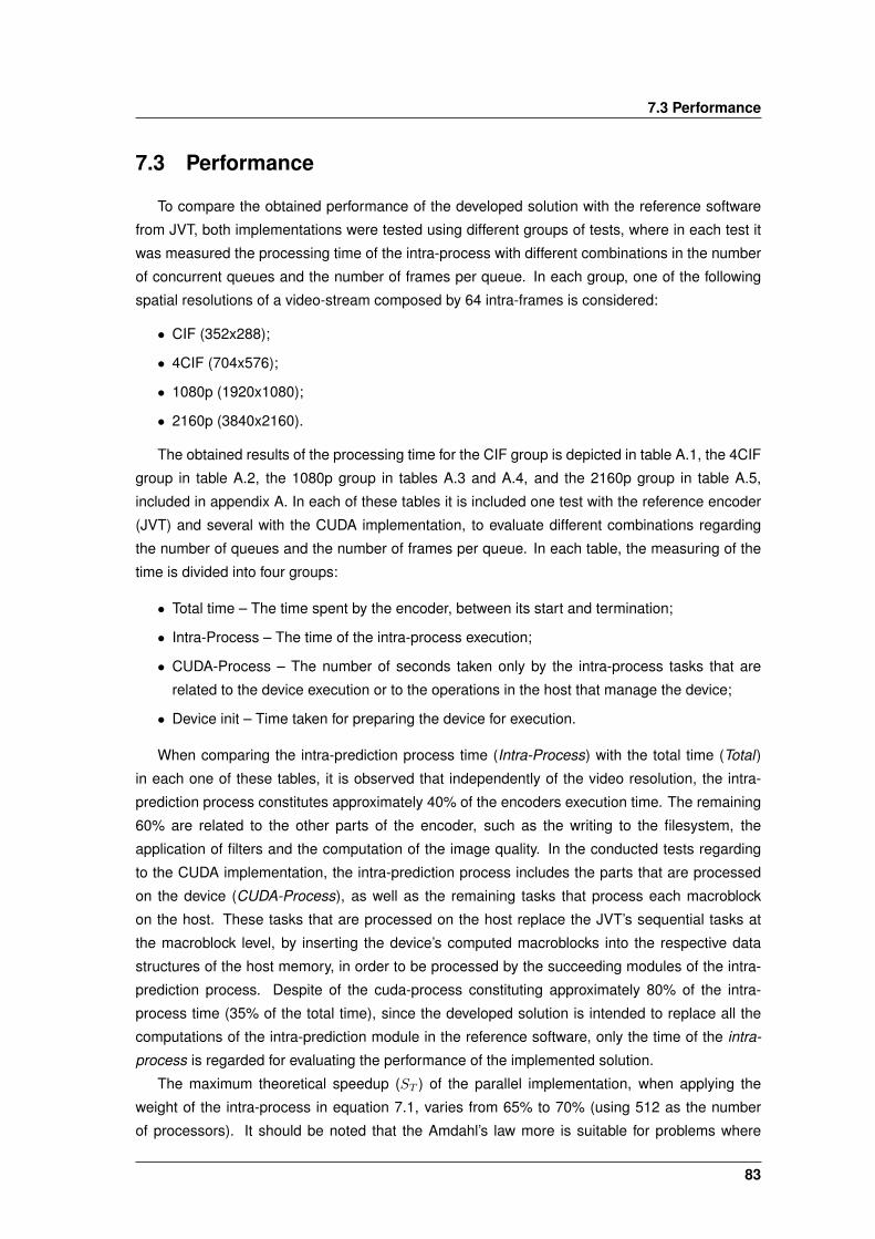
7.3 Performance
7.3 Performance
To compare the obtained performance of the developed solution with the reference software
from JVT, both implementations were tested using different groups of tests, where in each test it
was measured the processing time of the intra-process with different combinations in the number
of concurrent queues and the number of frames per queue. In each group, one of the following
spatial resolutions of a video-stream composed by 64 intra-frames is considered:
• CIF (352x288);
• 4CIF (704x576);
• 1080p (1920x1080);
• 2160p (3840x2160).
The obtained results of the processing time for the CIF group is depicted in table A.1, the 4CIF
group in table A.2, the 1080p group in tables A.3 and A.4, and the 2160p group in table A.5,
included in appendix A. In each of these tables it is included one test with the reference encoder
(JVT) and several with the CUDA implementation, to evaluate different combinations regarding
the number of queues and the number of frames per queue. In each table, the measuring of the
time is divided into four groups:
• Total time – The time spent by the encoder, between its start and termination;
• Intra-Process – The time of the intra-process execution;
• CUDA-Process – The number of seconds taken only by the intra-process tasks that are
related to the device execution or to the operations in the host that manage the device;
• Device init – Time taken for preparing the device for execution.
When comparing the intra-prediction process time (Intra-Process) with the total time (Total)
in each one of these tables, it is observed that independently of the video resolution, the intra-
prediction process constitutes approximately 40% of the encoders execution time. The remaining
60% are related to the other parts of the encoder, such as the writing to the filesystem, the
application of filters and the computation of the image quality. In the conducted tests regarding
to the CUDA implementation, the intra-prediction process includes the parts that are processed
on the device (CUDA-Process), as well as the remaining tasks that process each macroblock
on the host. These tasks that are processed on the host replace the JVT’s sequential tasks at
the macroblock level, by inserting the device’s computed macroblocks into the respective data
structures of the host memory, in order to be processed by the succeeding modules of the intra-
prediction process. Despite of the cuda-process constituting approximately 80% of the intra-
process time (35% of the total time), since the developed solution is intended to replace all the
computations of the intra-prediction module in the reference software, only the time of the intra-
process is regarded for evaluating the performance of the implemented solution.
The maximum theoretical speedup (ST ) of the parallel implementation, when applying the
weight of the intra-process in equation 7.1, varies from 65% to 70% (using 512 as the number
of processors). It should be noted that the Amdahl’s law more is suitable for problems where
83
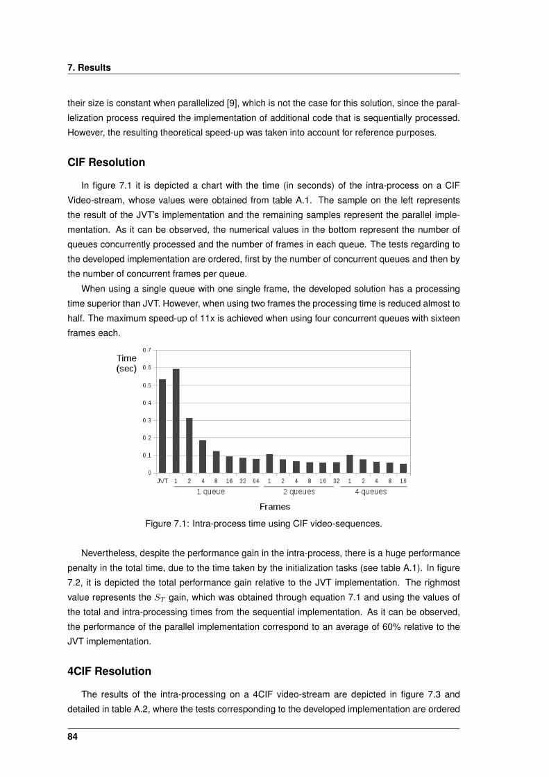
7. Results
their size is constant when parallelized [9], which is not the case for this solution, since the paral-
lelization process required the implementation of additional code that is sequentially processed.
However, the resulting theoretical speed-up was taken into account for reference purposes.
CIF Resolution
In figure 7.1 it is depicted a chart with the time (in seconds) of the intra-process on a CIF
Video-stream, whose values were obtained from table A.1. The sample on the left represents
the result of the JVT’s implementation and the remaining samples represent the parallel imple-
mentation. As it can be observed, the numerical values in the bottom represent the number of
queues concurrently processed and the number of frames in each queue. The tests regarding to
the developed implementation are ordered, first by the number of concurrent queues and then by
the number of concurrent frames per queue.
When using a single queue with one single frame, the developed solution has a processing
time superior than JVT. However, when using two frames the processing time is reduced almost to
half. The maximum speed-up of 11x is achieved when using four concurrent queues with sixteen
frames each.
Figure 7.1: Intra-process time using CIF video-sequences.
Nevertheless, despite the performance gain in the intra-process, there is a huge performance
penalty in the total time, due to the time taken by the initialization tasks (see table A.1). In figure
7.2, it is depicted the total performance gain relative to the JVT implementation. The righmost
value represents the ST gain, which was obtained through equation 7.1 and using the values of
the total and intra-processing times from the sequential implementation. As it can be observed,
the performance of the parallel implementation correspond to an average of 60% relative to the
JVT implementation.
4CIF Resolution
The results of the intra-processing on a 4CIF video-stream are depicted in figure 7.3 and
detailed in table A.2, where the tests corresponding to the developed implementation are ordered
84
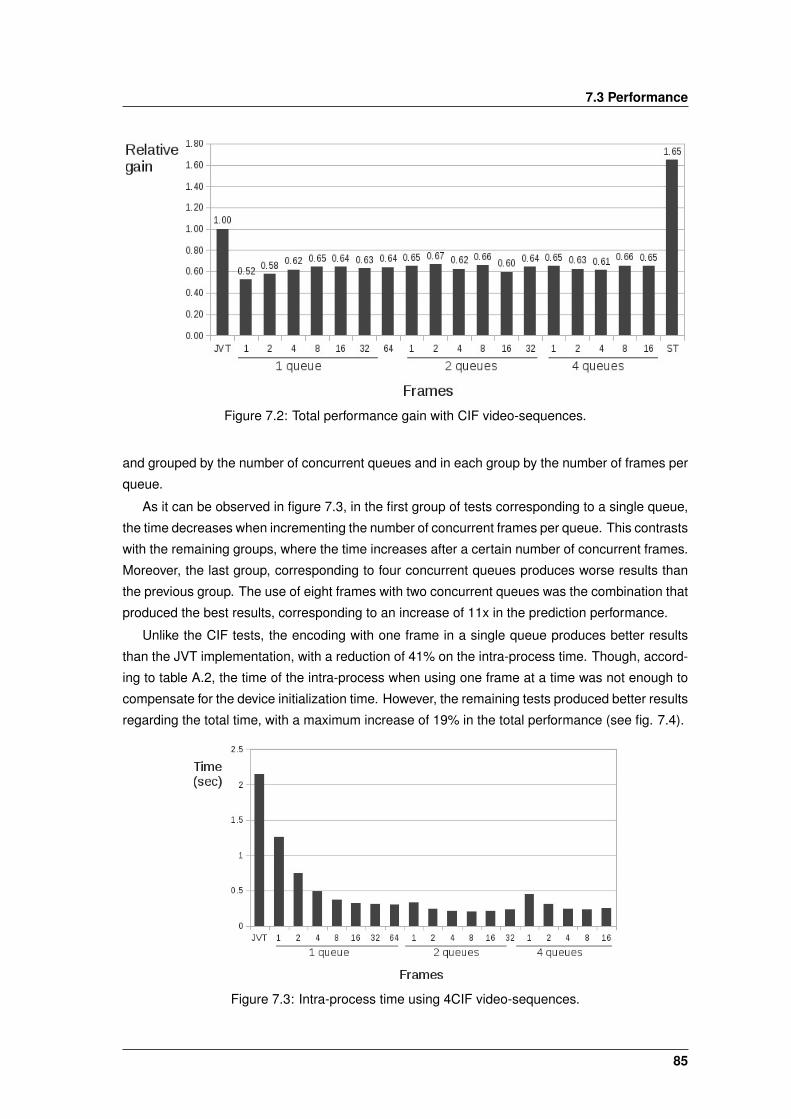
7.3 Performance
Figure 7.2: Total performance gain with CIF video-sequences.
and grouped by the number of concurrent queues and in each group by the number of frames per
queue.
As it can be observed in figure 7.3, in the first group of tests corresponding to a single queue,
the time decreases when incrementing the number of concurrent frames per queue. This contrasts
with the remaining groups, where the time increases after a certain number of concurrent frames.
Moreover, the last group, corresponding to four concurrent queues produces worse results than
the previous group. The use of eight frames with two concurrent queues was the combination that
produced the best results, corresponding to an increase of 11x in the prediction performance.
Unlike the CIF tests, the encoding with one frame in a single queue produces better results
than the JVT implementation, with a reduction of 41% on the intra-process time. Though, accord-
ing to table A.2, the time of the intra-process when using one frame at a time was not enough to
compensate for the device initialization time. However, the remaining tests produced better results
regarding the total time, with a maximum increase of 19% in the total performance (see fig. 7.4).
Figure 7.3: Intra-process time using 4CIF video-sequences.
85
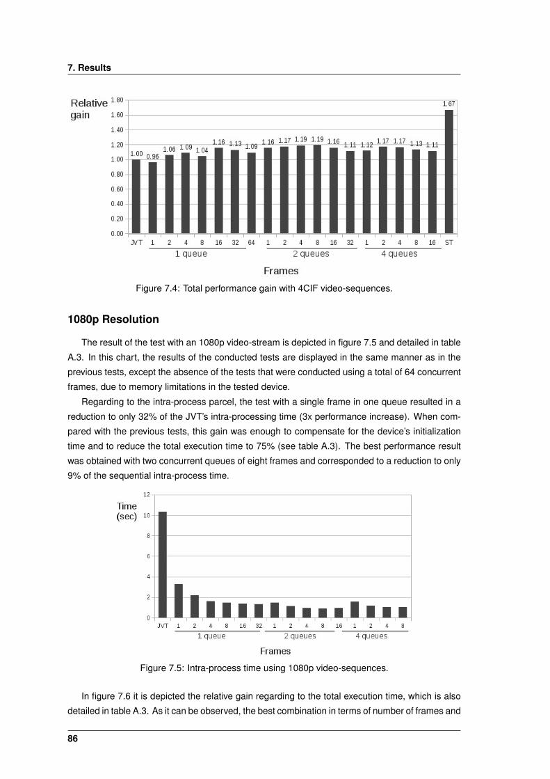
7. Results
Figure 7.4: Total performance gain with 4CIF video-sequences.
1080p Resolution
The result of the test with an 1080p video-stream is depicted in figure 7.5 and detailed in table
A.3. In this chart, the results of the conducted tests are displayed in the same manner as in the
previous tests, except the absence of the tests that were conducted using a total of 64 concurrent
frames, due to memory limitations in the tested device.
Regarding to the intra-process parcel, the test with a single frame in one queue resulted in a
reduction to only 32% of the JVT’s intra-processing time (3x performance increase). When com-
pared with the previous tests, this gain was enough to compensate for the device’s initialization
time and to reduce the total execution time to 75% (see table A.3). The best performance result
was obtained with two concurrent queues of eight frames and corresponded to a reduction to only
9% of the sequential intra-process time.
Figure 7.5: Intra-process time using 1080p video-sequences.
In figure 7.6 it is depicted the relative gain regarding to the total execution time, which is also
detailed in table A.3. As it can be observed, the best combination in terms of number of frames and
86
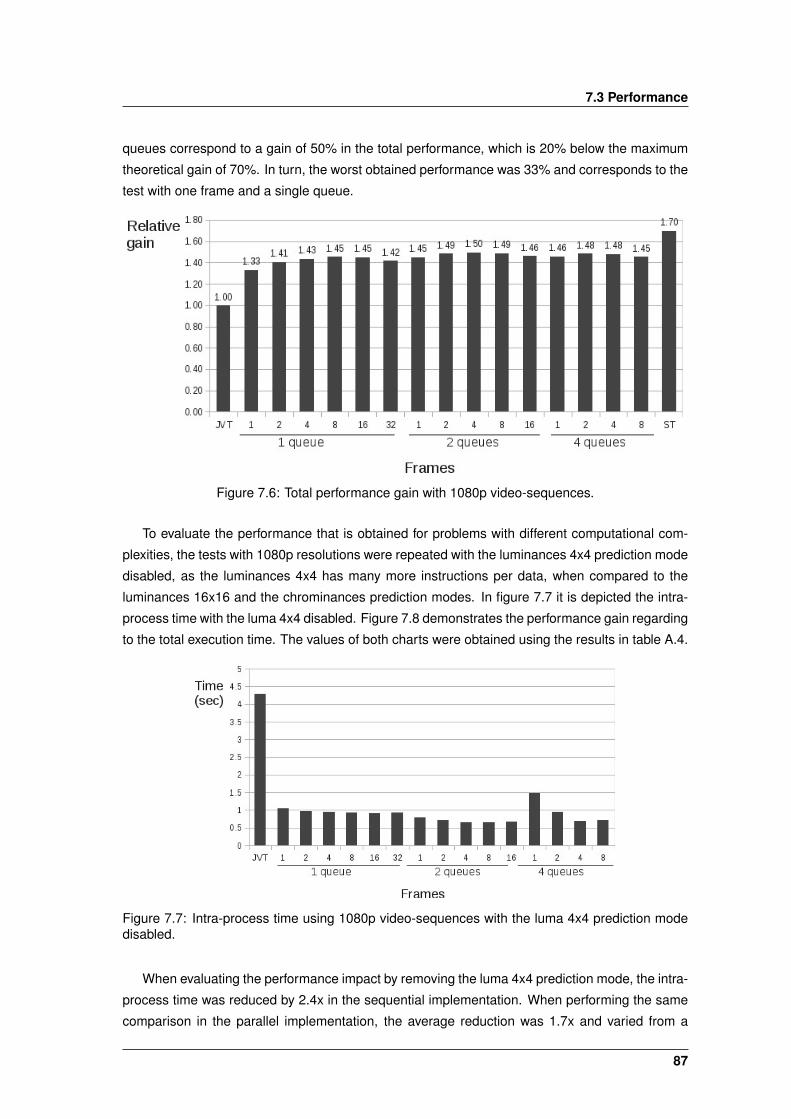
7.3 Performance
queues correspond to a gain of 50% in the total performance, which is 20% below the maximum
theoretical gain of 70%. In turn, the worst obtained performance was 33% and corresponds to the
test with one frame and a single queue.
Figure 7.6: Total performance gain with 1080p video-sequences.
To evaluate the performance that is obtained for problems with different computational com-
plexities, the tests with 1080p resolutions were repeated with the luminances 4x4 prediction mode
disabled, as the luminances 4x4 has many more instructions per data, when compared to the
luminances 16x16 and the chrominances prediction modes. In figure 7.7 it is depicted the intra-
process time with the luma 4x4 disabled. Figure 7.8 demonstrates the performance gain regarding
to the total execution time. The values of both charts were obtained using the results in table A.4.
Figure 7.7: Intra-process time using 1080p video-sequences with the luma 4x4 prediction modedisabled.
When evaluating the performance impact by removing the luma 4x4 prediction mode, the intra-
process time was reduced by 2.4x in the sequential implementation. When performing the same
comparison in the parallel implementation, the average reduction was 1.7x and varied from a
87
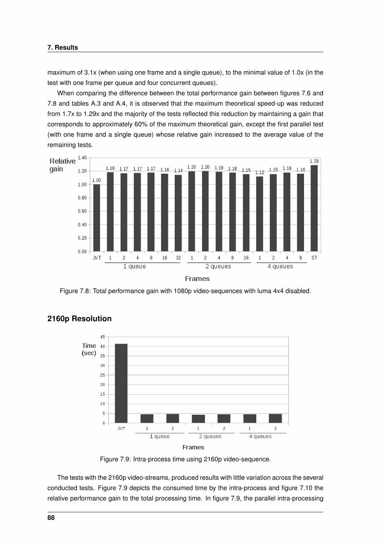
7. Results
maximum of 3.1x (when using one frame and a single queue), to the minimal value of 1.0x (in the
test with one frame per queue and four concurrent queues).
When comparing the difference between the total performance gain between figures 7.6 and
7.8 and tables A.3 and A.4, it is observed that the maximum theoretical speed-up was reduced
from 1.7x to 1.29x and the majority of the tests reflected this reduction by maintaining a gain that
corresponds to approximately 60% of the maximum theoretical gain, except the first parallel test
(with one frame and a single queue) whose relative gain increased to the average value of the
remaining tests.
Figure 7.8: Total performance gain with 1080p video-sequences with luma 4x4 disabled.
2160p Resolution
Figure 7.9: Intra-process time using 2160p video-sequence.
The tests with the 2160p video-streams, produced results with little variation across the several
conducted tests. Figure 7.9 depicts the consumed time by the intra-process and figure 7.10 the
relative performance gain to the total processing time. In figure 7.9, the parallel intra-processing
88
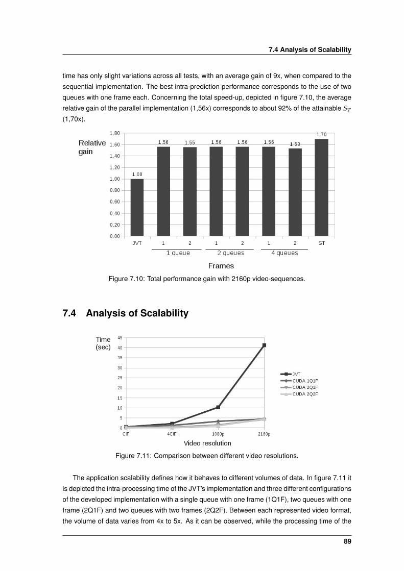
7.4 Analysis of Scalability
time has only slight variations across all tests, with an average gain of 9x, when compared to the
sequential implementation. The best intra-prediction performance corresponds to the use of two
queues with one frame each. Concerning the total speed-up, depicted in figure 7.10, the average
relative gain of the parallel implementation (1,56x) corresponds to about 92% of the attainable ST
(1,70x).
Figure 7.10: Total performance gain with 2160p video-sequences.
7.4 Analysis of Scalability
Figure 7.11: Comparison between different video resolutions.
The application scalability defines how it behaves to different volumes of data. In figure 7.11 it
is depicted the intra-processing time of the JVT’s implementation and three different configurations
of the developed implementation with a single queue with one frame (1Q1F), two queues with one
frame (2Q1F) and two queues with two frames (2Q2F). Between each represented video format,
the volume of data varies from 4x to 5x. As it can be observed, while the processing time of the
89

7. Results
sequential implementation has a proportional variation to the volume of data, in the developed
parallel implementations, the processing time increases at a rate much lower. In the developed
implementation, it is also observed that the configuration of one frame and a single queue has the
highest growing rate until the 1080p format and the lowest growing rate until the 2160p format.
This behaviour demonstrates that the GPU resources are only fully utilized in these tests, with
the 1080p and 2160p video formats. This also demonstrates the scalability of the implemented
solution for video formats with resolutions higher than 2160p.
7.5 Discussion
The performance of the developed solution is influenced by several aspects, such as memory
transfers, organization and management of tasks, or the relation between the number of compu-
tations and the volume of data in which these computations are performed.
From the previous results, it is observed that the processing time of the several parallel imple-
mentations has different values, when compared to its sequential counterpart. Regarding to the
intra-prediction process, the volume of data corresponding to a single frame with the CIF reso-
lution is not sufficient to mitigate the latency imposed by the memory transfers between the host
and the device memory spaces. Concerning the total execution time, the to results presented
in table A.1 demonstrate that to outperform the sequential implementation it would be required a
video sequence with at least twice the length of the video sequence used in the tests, as the time
taken by the sequential implementation to process 64 frames is nearly identical to the time taken
just to initialize the CUDA device.
It was also observed that when increasing the volume of data delivered to the GPU for pro-
cessing, the processing time tends to decrease until a certain amount of data, from which it starts
to increase slowly. This turning point marks the exact volume of data required to be processed in
the device with the maximum efficiency. The GPU resources are being wasted below this point,
and starting to be overloaded above it. Nevertheless, in figure 7.11 it can be noticed the difference
in the observed scalability between the sequential and the CUDA implementation, where the later
is much more scalable then the former.
In figure 7.6, it can be observed a small discrepancy in the tests regarding the parallel imple-
mentation, between the test with only one frame and a single queue, and the remaining tests.
While the first test achieves a gain of 33%, the remaining tests achieve a gain of averagely 46%.
However, this discrepancy is not verified in figure 7.8, which respects to the tests with the luma 4x4
intra-prediction mode disabled. This demonstrates the limitation of the GPU to perform complex
computations. Moreover, since the luma 4x4 intra-prediction is computed on the GPU with low
parallelism, which in turn is compensated by using more instructions per thread, this behaviour
tends to be contradictory to [40] regarding the performance with low parallelism. It should be
noted that this discrepancy is only verified in the tests with a single frame and a single queue,
as this effect is not observed by the remaining tasks, where the low parallelism is hidden by the
concurrency of multiple frames.
90

8Conclusions and Future Work
Contents8.1 Conclusions . . . . . . . . . . . . . . . . . . . . . . . . . . . . . . . . . . . . . . 928.2 Future Work . . . . . . . . . . . . . . . . . . . . . . . . . . . . . . . . . . . . . . 93
91
8. Conclusions and Future Work
The purpose of this work was to develop a parallel implementation of the intra-prediction and
encoding module of the H.264/AVC standard, by using the computational resources of a GPU.
One of the considered requisites was the integration of the developed solution to be in an existing
implementation, where the intra-prediction was originally processed sequentially.
The development process essentially consisted in mapping tasks, which had been optimized
to be sequentially processed, into data-parallel tasks. As the existing sequential tasks could not
be straightforwardly implemented, the process of mapping required a great effort by following a
bottom-up approach, where each task was decomposed and reimplemented in a data-parallel
fashion.
The developed solution resulted in a module that can be easily integrated in the original se-
quential implementation and can be replaced at run time whenever a CUDA device is available.
Regarding to the intra-prediction, the developed solution supports the 4x4 and the 16x16 pre-
diction modes of the luminances and the 8x8 modes of the chrominances. It is also capable of
processing any spatial resolution of the video sequences from CIF and HD video formats.
8.1 Conclusions
The developed solution proved to be a viable and alternative approach to encode intra type
frames. As can be observed in the results section, the parallel implementation of the intra-
prediction module achieved a speedup of 11x, relatively to the sequential implementation of the
reference software.
By taking into account the obtained results, it can be concluded that the process of the intra-
prediction on the GPU resulted in a more scalable solution than a similar approach using exclu-
sively the multi-core capabilities of the CPU.
The proposed solution also proved to be adaptable to different video formats with different
spatial resolutions. By offloading the computations to the GPU in a pipeline scheme, the execution
cost of the the intra-prediction module could be mitigated, by allowing the remaining parts of the
encoder to be processed on the CPU, while the data elements required in the next iterations were
computed in advance by the GPU.
The possibility of processing the intra-prediction using macroblocks from several frames in par-
allel permits an efficient usage of the computing resources available in the GPU, by increasing the
number of processed frames in parallel to compensate for the sub-utilization of the computational
resources, when using video streams with low spatial resolutions.
Due to the negative impact of the long communication latency between the host the device
memory spaces, it was also concluded that there is a limit in the spatial resolution or in the number
of intra type frames processed in parallel to allow any performance gain with a GPU. Therefore,
according to the previous results, the video stream must have at least a 1080p spatial resolution
in order to process a single frame at a time in the GPU, or when processing CIF video streams,
at least as twice as the number of parallel frames used in the previous results (ex: at least 128
frames).
92
8.2 Future Work
8.2 Future Work
Taking into account the obtained results, the computing capabilities of the CUDA GPUs and the
remaining modules of the H.264 standard, there are still many possibilities to continue this work.
The developed solution can be extended into a hybrid solution, which combines the simultaneous
use of multi-core CPUs with the computing resources of multiple GPUs, by assigning the intra-
prediction and coding tasks in a load balanced Round-Robbin fashion to the CPUs and GPUs.
This solution can even be further extended by being implemented in a distributed environment
with the combination of MPI and CUDA [6].
Another possibility consist in the implementation of the developed solution with the OpenCL
API. Even though this API is somewhat more limited than CUDA, it is a technology that is evolving
and is supported by a larger diversity of computing devices.
Other possibility to continue this work consists in using the same design methodology to extend
the data-parallelism still available in other H.264 modules, such as the inter-prediction, which
not only is more demanding in terms of computational complexity, but also may allow a better
exploitation of the data-level parallelism.
Alternatively, the developed solution could also be extended to implement the intra-prediction
module in the recent High Efficiency Video Coding (HEVC) standard [27]. Despite being more
computational demanding than the H.264, due to its greater capabilities, the new NVIDIA GPUs
based on the Kepler architecture may offer greater compute capabilities and provide yet more
significant gains.
93
Bibliography
[1] Acharya, T. and Ray, A. K. (2005). Image Processing Principles and Applications. Wiley.
[2] Bialkowski, J., Kaup, A., and Illgner, K. (2004). Fast transcoding of intra frames between H.263
and H.264. In Image Processing, 2004. ICIP ’04. 2004 International Conference on, volume 4,
pages 2785 – 2788 Vol. 4.
[3] Bovik, A. (2009). The Essential Guide to Video Processing. Academic Press.
[4] Cheung, N.-M., Au, O., Kung, M.-C., Wong, P., and Liu, C. H. (2009). Highly Parallel Rate-
Distortion Optimized Intra-Mode Decision on Multicore Graphics Processors. Circuits and
Systems for Video Technology, IEEE Transactions on, 19(11):1692 –1703.
[5] Cheung, N.-M., Fan, X., Au, O., and Kung, M.-C. (2010). Video Coding on Multicore Graphics
Processors. Signal Processing Magazine, IEEE, 27(2):79 –89.
[6] Farber, R. (2011). CUDA Application Design and Development. Morgan Kaufman.
[7] Foster, I. (1995). Designing and Building Parallel Programs. Addison Wesley.
[8] Glaskowsky, P. (2009). Nvidia’s fermi: the first complete gpu computing architecture. NVIDIA.
[9] Gustafson, J. (1988). Reevaluating amdahl’s law. Communications of the ACM, 31(5):532–
533.
[10] Hanzo, L., Cherriman, P. J., and Streit, J. (2007). Video Compression and Communications.
Wiley.
[11] Herlihy, M. and Shavit, N. (2008). The Art of Multiprocessor Programming. Morgan Kauf-
mann.
[12] Jin, G. and Lee, H.-J. (2006). A Parallel and Pipelined Execution of H.264/AVC Intra Pre-
diction. In Computer and Information Technology, 2006. CIT ’06. The Sixth IEEE International
Conference on, page 246.
[13] Kirk, D. B. and mei W. Hwu, W. (2010). Programming Massively Parallel Processors. Morgan
Kaufmann.
[14] Kung, M., Au, O., Wong, P., and Liu, C.-H. (2007). Intra Frame Encoding Using Pro-
grammable Graphics Hardware. In Advances in Multimedia Information Processing – PCM
2007, volume 4810 of Lecture Notes in Computer Science, pages 609–618. Springer Berlin /
Heidelberg.
94
Bibliography
[15] Lee, W., Lee, S., and Kim, J. (2006). Pipelined Intra Prediction Using Shuffled Encoding
Order for H.264/AVC. In TENCON 2006. 2006 IEEE Region 10 Conference, pages 1 –4.
[16] Lindholm, E., Nickolls, J., Oberman, S., and Montrym, J. (2008). NVIDIA Tesla: A Unified
Graphics and Computing Architecture. Micro, IEEE, 28(2):39 –55.
[17] Malvar, H., Hallapuro, A., Karczewicz, M., and Kerofsky, L. (2003). Low-complexity transform
and quantization in h.264/avc. Circuits and Systems for Video Technology, IEEE Transactions
on, 13(7):598 – 603.
[18] Mattson, T. G., Sanders, B. A., and Massingill, B. L. (2010).
Patterns for Parallel Programming. Addison-Wesley.
[19] Nickolls, J. and Dally, W. (2010). The GPU Computing Era. Micro, IEEE, 30(2):56 –69.
[20] NVIDIA (2009). NVIDIA Fermi Compute Architecture Whitepaper. http://www.nvidia.com/
content/PDF/fermi_white_papers/NVIDIA_Fermi_Compute_Architecture_Whitepaper.
pdf. Retrieved on September 01, 2012.
[21] NVIDIA (2011). The CUDA Compiler Driver NVCC. http://developer.download.nvidia.
com/compute/DevZone/docs/html/C/doc/nvcc.pdf. Retrieved on September 01, 2012.
[22] NVIDIA (2012a). CUDA API Reference Manual, Version 4.2. http://developer.download.
nvidia.com/compute/DevZone/docs/html/C/doc/CUDA_Toolkit_Reference_Manual.pdf.
Retrieved September 01, 2012.
[23] NVIDIA (2012b). CUDA C Best Practices Guide, Version 4.1. http://developer.download.
nvidia.com/compute/DevZone/docs/html/C/doc/CUDA_C_Best_Practices_Guide.pdf. Re-
trieved September 01, 2012.
[24] NVIDIA (2012c). NVIDIA CUDA C Programming Guide, Version 4.2. http:
//developer.download.nvidia.com/compute/DevZone/docs/html/C/doc/CUDA_C_
Programming_Guide.pdf. Retrieved September 01, 2012.
[25] NVIDIA (2012d). Parallel Thread Execution, ISA Version 3.0. http://developer.download.
nvidia.com/compute/DevZone/docs/html/C/doc/ptx_isa_3.0.pdf. Retrieved September
01, 2012.
[26] Ostermann, J., Bormans, J., List, P., Marpe, D., Narroschke, M., Pereira, F., Stockhammer,
T., and Wedi, T. (2004). Video coding with H.264/AVC: tools, performance, and complexity.
Circuits and Systems Magazine, IEEE, 4(1):7 – 28.
[27] Pourazad, M., Doutre, C., Azimi, M., and Nasiopoulos, P. (2012). Hevc: The new gold stan-
dard for video compression: How does hevc compare with h. 264/avc? Consumer Electronics
Magazine, IEEE, 1(3):36–46.
[28] Richardson, I. E. G. (2002). The H.264 Advanced Video Compression Standard. Wiley,
second edition.
95
Bibliography
[29] Richardson, I. E. G. (2003). H.264 and MPEG-4 Video Compression: Video Coding for
Next-generation Multimedia. Wiley.
[30] Roma, N. and Sousa, L. (2011). A tutorial overview on the properties of the discrete cosine
transform for encoded image and video processing. Signal Processing, 91(11):2443 – 2464.
[31] Sanders, J. and Kandrot, E. (2010). CUDA by Example. Addison Wesley.
[32] Santos, L., Lopez, S., Callico, G., Lopez, J., and Sarmiento, R. (2012). Performance
evaluation of the h. 264/avc video coding standard for lossy hyperspectral image compres-
sion. Selected Topics in Applied Earth Observations and Remote Sensing, IEEE Journal of,
5(2):451–461.
[33] Scott, M. L. (2009). Programming Language Pragmantics. Morgan Kaufman, third edition.
[34] Siegel, J., Ributzka, J., and Li, X. (2009). Cuda memory optimizations for large data-
structures in the gravit simulator. In Parallel Processing Workshops, 2009. ICPPW ’09.
International Conference on, pages 174 –181.
[35] Simpson, W. (2008). Video Over IP: IPTV, Internet Video, H.264, P2P, Web TV, and
Streaming: A Complete Guide to Understanding the Technology. Focal Press, second edition.
[36] Su, R., Liu, G., and Zhang, T. (2006). Fast Mode Decision Algorithm for Intra Prediction in
H.264/AVC. In Acoustics, Speech and Signal Processing, 2006. ICASSP 2006 Proceedings.
2006 IEEE International Conference on, volume 2, page II.
[37] T., W. (2003). Draft itu-t recommendation and final draft international standard of joint video
specification. ITU-T rec. H.264—ISO/IEC 14496-10 AVC.
[38] Torres, Y., Gonzalez-Escribano, A., and Llanos, D. (2011). Understanding the impact of cuda
tuning techniques for fermi. In High Performance Computing and Simulation (HPCS), 2011
International Conference on, pages 631 –639.
[39] Tourapis, A. M., Leontaris, A., Suhring, K., and Sullivan, G. (2009). H.264/14496-10 AVC
Reference Software Manual. In Joint Video Team (JVT) of ISO/IEC MPEG & ITU-T VCEG
(ISO/IEC JTC1/SC29/WG11 and ITU-T SG16 Q.6). Joint Video Team (JVT).
[40] Volkov, V. (2010). Better performance at lower occupancy. In Proceedings of the GPU
Technology Conference, GTC, volume 10.
[41] Wiegand, T., Sullivan, G., Bjontegaard, G., and Luthra, A. (2003). Overview of the H.264/AVC
video coding standard. Circuits and Systems for Video Technology, IEEE Transactions on,
13(7):560 –576.
[42] Zhang, Y., Jiang, G., Yi, W., Yu, M., Li, F., Jiang, Z., and Liu, W. (2006). An Improved Design
of Quantization for H.264 Video Coding Standard. In Signal Processing, 2006 8th International
Conference on, volume 2.
96

AAppendix A
97
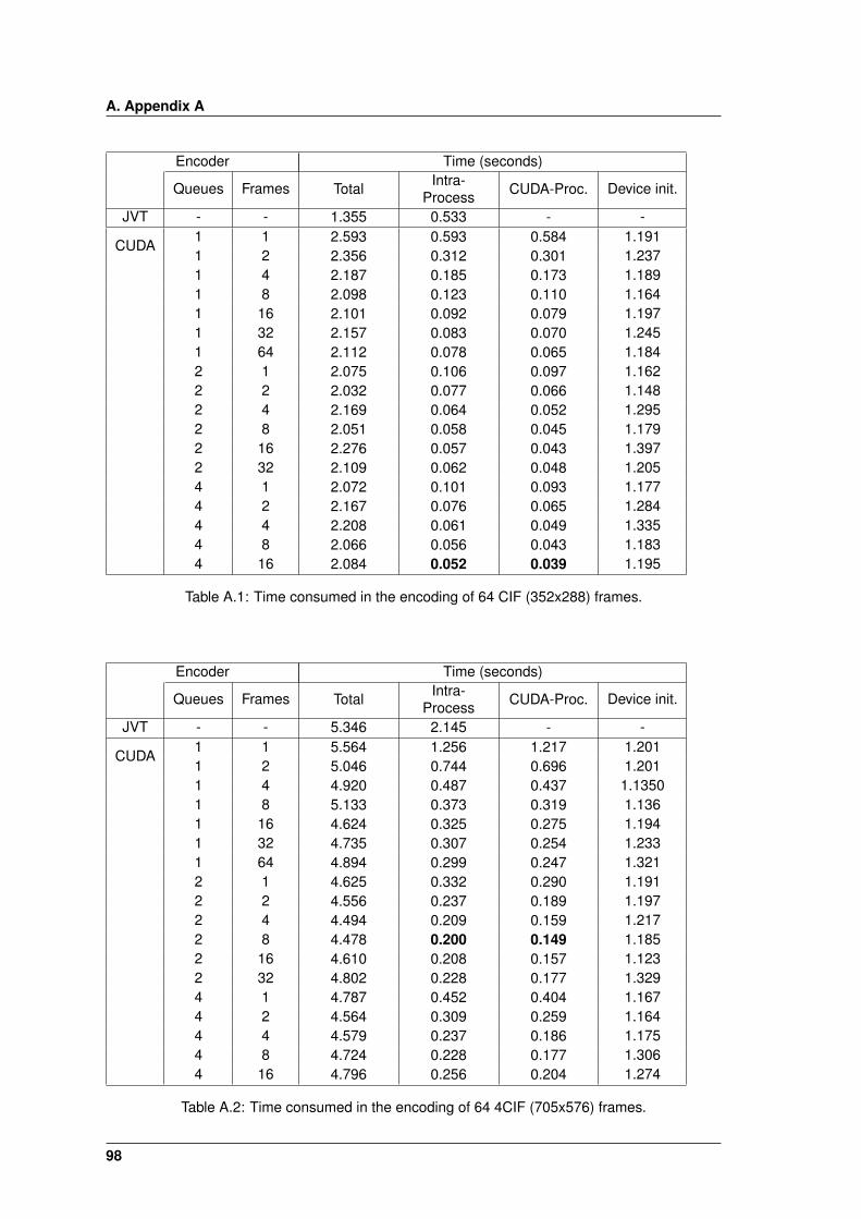
A. Appendix A
Encoder Time (seconds)
Queues Frames Total Intra-Process CUDA-Proc. Device init.
JVT - - 1.355 0.533 - -
CUDA1 1 2.593 0.593 0.584 1.1911 2 2.356 0.312 0.301 1.2371 4 2.187 0.185 0.173 1.1891 8 2.098 0.123 0.110 1.1641 16 2.101 0.092 0.079 1.1971 32 2.157 0.083 0.070 1.2451 64 2.112 0.078 0.065 1.1842 1 2.075 0.106 0.097 1.1622 2 2.032 0.077 0.066 1.1482 4 2.169 0.064 0.052 1.2952 8 2.051 0.058 0.045 1.1792 16 2.276 0.057 0.043 1.3972 32 2.109 0.062 0.048 1.2054 1 2.072 0.101 0.093 1.1774 2 2.167 0.076 0.065 1.2844 4 2.208 0.061 0.049 1.3354 8 2.066 0.056 0.043 1.1834 16 2.084 0.052 0.039 1.195
Table A.1: Time consumed in the encoding of 64 CIF (352x288) frames.
Encoder Time (seconds)
Queues Frames Total Intra-Process CUDA-Proc. Device init.
JVT - - 5.346 2.145 - -
CUDA1 1 5.564 1.256 1.217 1.2011 2 5.046 0.744 0.696 1.2011 4 4.920 0.487 0.437 1.13501 8 5.133 0.373 0.319 1.1361 16 4.624 0.325 0.275 1.1941 32 4.735 0.307 0.254 1.2331 64 4.894 0.299 0.247 1.3212 1 4.625 0.332 0.290 1.1912 2 4.556 0.237 0.189 1.1972 4 4.494 0.209 0.159 1.2172 8 4.478 0.200 0.149 1.1852 16 4.610 0.208 0.157 1.1232 32 4.802 0.228 0.177 1.3294 1 4.787 0.452 0.404 1.1674 2 4.564 0.309 0.259 1.1644 4 4.579 0.237 0.186 1.1754 8 4.724 0.228 0.177 1.3064 16 4.796 0.256 0.204 1.274
Table A.2: Time consumed in the encoding of 64 4CIF (705x576) frames.
98
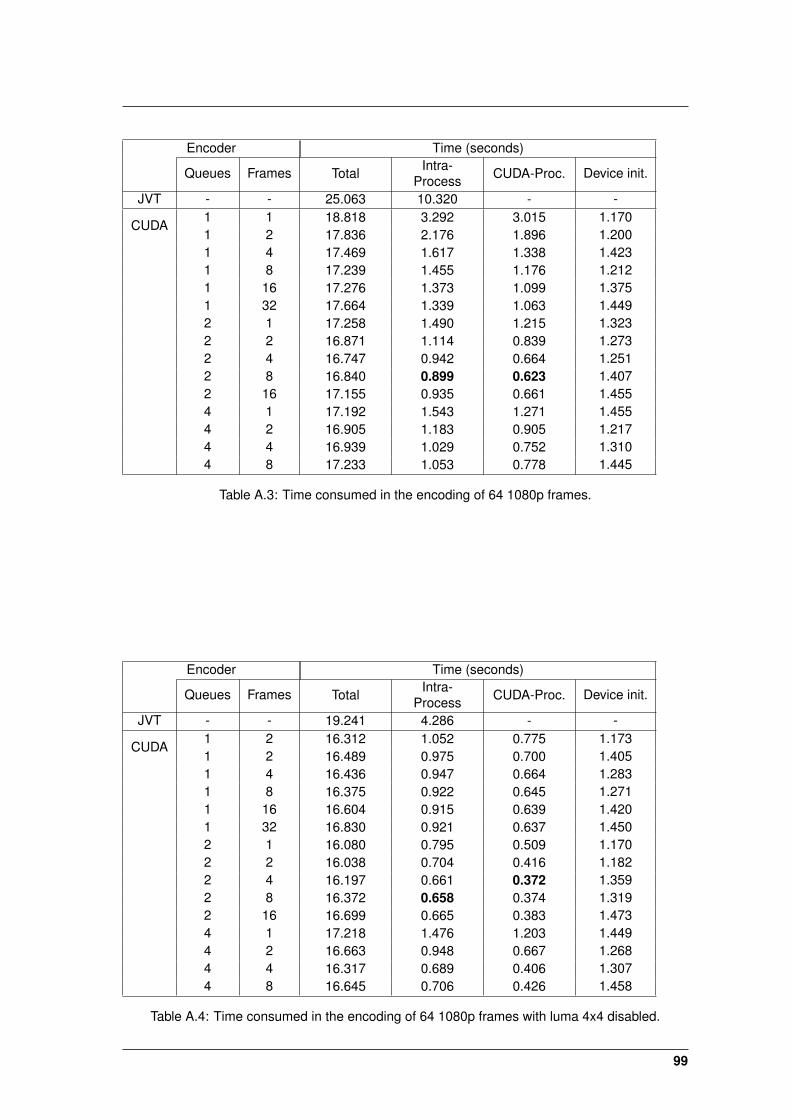
Encoder Time (seconds)
Queues Frames Total Intra-Process CUDA-Proc. Device init.
JVT - - 25.063 10.320 - -
CUDA1 1 18.818 3.292 3.015 1.1701 2 17.836 2.176 1.896 1.2001 4 17.469 1.617 1.338 1.4231 8 17.239 1.455 1.176 1.2121 16 17.276 1.373 1.099 1.3751 32 17.664 1.339 1.063 1.4492 1 17.258 1.490 1.215 1.3232 2 16.871 1.114 0.839 1.2732 4 16.747 0.942 0.664 1.2512 8 16.840 0.899 0.623 1.4072 16 17.155 0.935 0.661 1.4554 1 17.192 1.543 1.271 1.4554 2 16.905 1.183 0.905 1.2174 4 16.939 1.029 0.752 1.3104 8 17.233 1.053 0.778 1.445
Table A.3: Time consumed in the encoding of 64 1080p frames.
Encoder Time (seconds)
Queues Frames Total Intra-Process CUDA-Proc. Device init.
JVT - - 19.241 4.286 - -
CUDA1 2 16.312 1.052 0.775 1.1731 2 16.489 0.975 0.700 1.4051 4 16.436 0.947 0.664 1.2831 8 16.375 0.922 0.645 1.2711 16 16.604 0.915 0.639 1.4201 32 16.830 0.921 0.637 1.4502 1 16.080 0.795 0.509 1.1702 2 16.038 0.704 0.416 1.1822 4 16.197 0.661 0.372 1.3592 8 16.372 0.658 0.374 1.3192 16 16.699 0.665 0.383 1.4734 1 17.218 1.476 1.203 1.4494 2 16.663 0.948 0.667 1.2684 4 16.317 0.689 0.406 1.3074 8 16.645 0.706 0.426 1.458
Table A.4: Time consumed in the encoding of 64 1080p frames with luma 4x4 disabled.
99
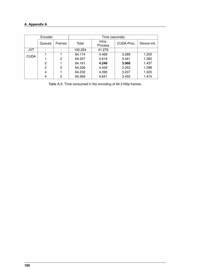
A. Appendix A
Encoder Time (seconds)
Queues Frames Total Intra-Process CUDA-Proc. Device init.
JVT - - 100.254 41.279 - -
CUDA1 1 64.174 4.469 3.289 1.2001 2 64.507 4.619 3.441 1.3822 1 64.161 4.248 3.068 1.4372 2 64.206 4.429 3.253 1.2984 1 64.232 4.390 3.207 1.3204 2 65.569 4.641 3.455 1.415
Table A.5: Time consumed in the encoding of 64 2160p frames.
100

101