Video Enhancement Using Per-Pixel Virtual ExposuresEric P. Bennett Leonard McMillan

The University of North Carolina at Chapel Hill

Abstract We enhance underexposed, low dynamic range videos by adaptively and independently varying the exposure at each photoreceptor in a post-process. This virtual exposure is a dynamic function of both the spatial neighborhood and temporal history at each pixel. Temporal integration enables us to expand the image’s dynamic range while simultaneously reducing noise. Our non-linear exposure variation and denoising filters smoothly transition from temporal to spatial for moving scene elements. Our virtual exposure framework also supports temporally coherent per frame tone mapping. Our system outputs restored video sequences with significantly reduced noise, increased exposure time of dark pixels, intact motion, and improved details. CR Categories: I.4.3: Image Processing and Computer Vision – enhancement, filtering. I.3.3: Computer Graphics – picture/image generation, display algorithms. Keywords: Digital video, Noise reduction, Low dynamic range, Exposure, Bilateral filter, Restoration, Tone mapping.

1 Introduction Alternatively, HDR images can be assembled by additively combining multiple uniformly exposed digital images [Liu et al 03] [Jostschulte et al 98]. This approach is particularly compatible with digital video, but it has been largely overlooked since it requires processing O(N) source images compared to the O(log(N)) of variable exposure methods. Nevertheless, the combination of multiple uniformly exposed images affords certain advantages, including noise reduction. Moreover, if one varies the number of uniformly exposed images combined on a pixel-by-pixel basis, it becomes possible to adjust each pixel’s exposure independently, allowing for direct tone mapping without explicit construction of an intermediate HDR image. Local exposure control also provides a tool for handling dynamic scenes. This approach constitutes our Virtual Exposure Camera (VEC) conceptual model.

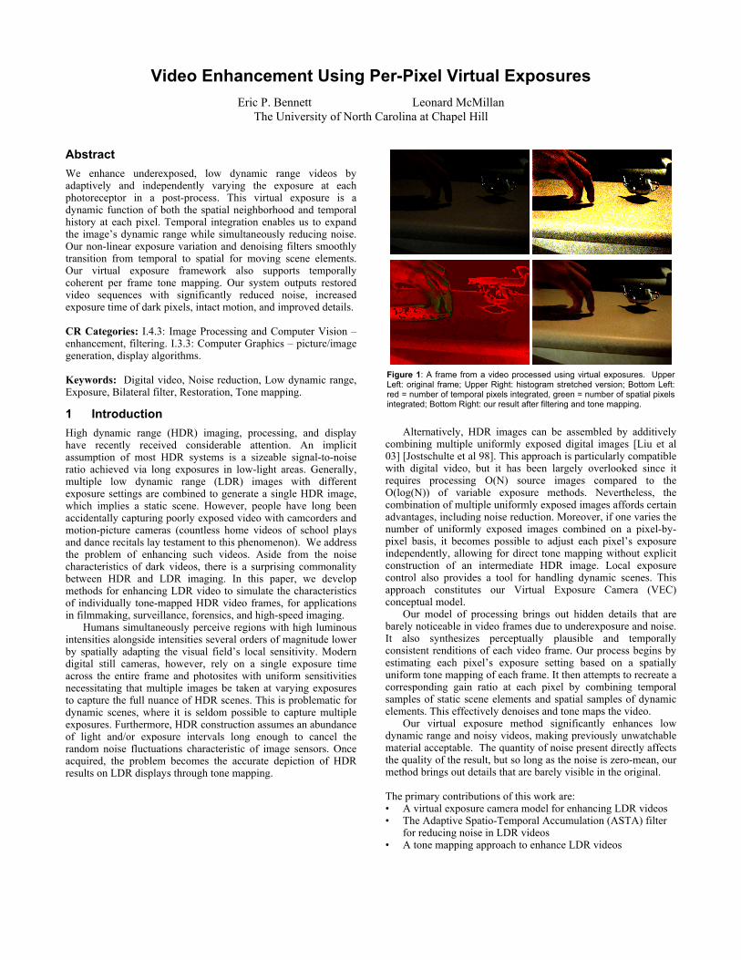
Figure 1: A frame from a video processed using virtual exposures. Upper Left: original frame; Upper Right: histogram stretched version; Bottom Left: red = number of temporal pixels integrated, green = number of spatial pixels integrated; Bottom Right: our result after filtering and tone mapping.

High dynamic range (HDR) imaging, processing, and display have recently received considerable attention. An implicit assumption of most HDR systems is a sizeable signal-to-noise ratio achieved via long exposures in low-light areas. Generally, multiple low dynamic range (LDR) images with different exposure settings are combined to generate a single HDR image, which implies a static scene. However, people have long been accidentally capturing poorly exposed video with camcorders and motion-picture cameras (countless home videos of school plays and dance recitals lay testament to this phenomenon). We address the problem of enhancing such videos. Aside from the noise characteristics of dark videos, there is a surprising commonality between HDR and LDR imaging. In this paper, we develop methods for enhancing LDR video to simulate the characteristics of individually tone-mapped HDR video frames, for applications in filmmaking, surveillance, forensics, and high-speed imaging. Our model of processing brings out hidden details that are

barely noticeable in video frames due to underexposure and noise. It also synthesizes perceptually plausible and temporally consistent renditions of each video frame. Our process begins by estimating each pixel’s exposure setting based on a spatially uniform tone mapping of each frame. It then attempts to recreate a corresponding gain ratio at each pixel by combining temporal samples of static scene elements and spatial samples of dynamic elements. This effectively denoises and tone maps the video.

Humans simultaneously perceive regions with high luminous intensities alongside intensities several orders of magnitude lower by spatially adapting the visual field’s local sensitivity. Modern digital still cameras, however, rely on a single exposure time across the entire frame and photosites with uniform sensitivities necessitating that multiple images be taken at varying exposures to capture the full nuance of HDR scenes. This is problematic for dynamic scenes, where it is seldom possible to capture multiple exposures. Furthermore, HDR construction assumes an abundance of light and/or exposure intervals long enough to cancel the random noise fluctuations characteristic of image sensors. Once acquired, the problem becomes the accurate depiction of HDR results on LDR displays through tone mapping.

Our virtual exposure method significantly enhances low dynamic range and noisy videos, making previously unwatchable material acceptable. The quantity of noise present directly affects the quality of the result, but so long as the noise is zero-mean, our method brings out details that are barely visible in the original.

The primary contributions of this work are: • A virtual exposure camera model for enhancing LDR videos • The Adaptive Spatio-Temporal Accumulation (ASTA) filter for reducing noise in LDR videos • A tone mapping approach to enhance LDR videos

Other video filtering approaches have appeared that use temporal filtering. Dubois and Sabri [84] performed nonlinear temporal noise filtering assisted by displacement estimation. Each pixel is combined temporally using a recursive low-pass temporal filter weighted by the reliability of the displacement estimate. This method requires well-exposed, easy-to-track video to correctly filter. Our method adapts from temporal to spatial filtering to be robust to tracking inaccuracies. Jostschulte et al [98] presented a spatio-temporal shot noise filter that first spatially and then temporally filters video while preserving edges that match a template set. A motion-sensing algorithm is used to vary the amount of temporal filtering. We prefer to only use temporal filtering when possible and adapt the mix of temporal and spatial filtering based on a tone-mapping objective and local motion characteristics. Acosta-Serafini et al [04] described an HDR camera that selectively resets a pixel based on a prediction of when it will saturate. The reset interval and the digitized pixel level combine to form a floating-point value. They primarily focused on high-speed, HDR sensing and do not specifically address low-light situations. Liu et al [03] combined high-speed samples to reduce noise and improve dynamic range. Their approach is similar, but much lower-level than ours. It depends on specific imaging device features such as high-speed non-destructive reads. It also relies mostly on linear filters, and uses only single pixel areas to detect motion. In contrast, our method uses bilateral filtering, considers a larger context for motion detection, and targets a tone-mapped objective. Bidermann et al [03] described an HDR high-speed CMOS imager platform with per-pixel ADCs and storage, which could use the Liu et al [03] algorithm and targets well-lit scenes.

2 Related Work Enhancing low-dynamic range images has much in common with HDR acquisition, processing, and display. HDR representations have long been recognized as essential for accurately modeling light transport [Ward 91]. More recently, Debevec and Malik [97] developed accurate methods for assembling HDR images from a series of still photographs with increasingly long exposure times. The problem of mapping an HDR image for display on devices with limited dynamic range was formalized by Tumblin and Rushmier [93], and has led to a variety of spatially uniform [Drago et al 03] and spatially varying [Tumblin and Turk 99] [Durand and Dorsey 02] [Fattal et al 02] tone mapping approaches. A variety of methods have been proposed to tone map HDR images so that the maximum amount of information is visible on a monitor. Retinex theory, such as in the multiscale Retinex [Jobson et al 97], suggests that a Gaussian-like kernel can be convolved at each point in the image and subtracted from the original image in log space, providing for a more “viewable” version of a still image. The advantage of the Retinex approach is that it is non-iterative, but it can generate unwanted edge blurring artifacts. Durand and Dorsey [02] built a similar system, but used an edge preserving bilateral filter to maintain sharp edges. Pattanaik et al [00] presented an approach that mimics the time dependent local adaptation of the human visual system. They also discussed temporal coherence to avoid introducing frame-by-frame tone mapping “flicker”. In gradient domain HDR compression [Fattal et al 02], the gradient of an image is attenuated and then reintegrated. They also described a modification for improving images that already use a display’s full dynamic range. Raskar et al [04] also used gradient domain methods, but to fuse day and night images together— adding daytime context to nighttime footage.

Recently, Eisemann and Durand [04] and Petschnigg et al [04] have developed methods to remove noise and improve the dynamic range of underexposed images by incorporating features derived from properly exposed “flash images”. The extent of noise removal depends on how well exposed a given region is in the flash image. Furthermore, the underlying luminance model used in the processing is not HDR, either explicitly (as in previous tone-mapping systems) or implicitly (as in our case). It is also unclear how to extend these methods to video sequences. The goal of our virtual exposure approach is similar to these methods, but we incorporate temporal information instead of flash image features to improve the exposure. Thus, the illuminations of our enhancements are consistent with the original source.

The idea of using multiple temporally adjacent frames to enhance knowledge about a pixel’s true or desired value was considered in Cohen et al [03]. Multiple images were registered and then each pixel of the output image was computed as a function of its temporal neighbors. HDR compression using this algorithm was also described. Sand and Teller [04] discussed a video matching method for aligning slightly different video sources. Specifically, it contains a robust system for frame-to-frame alignment. We handle moving cameras by warping spatio-temporal volumes as described by Bennett and McMillan [03]. There is a long history of noise filtering methods throughout the signal processing literature. We are most interested in edge-preserving filters from the anisotropic diffusion and bilateral filter families. Anisotropic diffusion of images [Perona and Malik 90] provides an iterative filtering method that adapts to the image’s gradient. Bilateral filtering [Tomasi and Manduchi 98] provides a single-step noise removal process that shares many visual and mathematical qualities with anisotropic diffusion [Barash 02]. However, both of these methods are designed for single images and not for videos. The Trilateral filter [Choudhury and Tumblin 03] builds on the bilateral filter model by biasing its kernel away from edges and dynamically choosing the kernel’s size in an attempt to model signals as piecewise linear rather than piecewise constant functions. Other modifications have been proposed to improve the standard bilateral filter’s ability to handle noise [Boomgaard and Weijer 02] [Francis and Jager 03]. We combine the attributes of median filters with the bilateral filter. A “bilateral median” filter was described by Francis and Jager [03], but it uses a weighted median for summation purposes, unlike ours that uses it to establish a similarity distance. Spatio-Temporal Anisotropic Diffusion [Lee et al 98] discussed the possibility of using a three dimensional kernel to remove noise from videos where time is handled similarly to the spatial dimensions.

Researchers have also constructed actual high dynamic range video capture systems. Kang et al [03] built a system based on a camera that could sequence through different exposure settings. Once the images were registered using optical flow, it was possible to combine exposures to improve the dynamic range. The small number of frames combined suggests that a high signal-to-noise ratio (SNR) was assumed, and therefore, it would only be useful for well-lit scenes. Nayar and Branzoi [03] presented a system whereby a computer controlled LCD panel was placed in front of the CCD. The per-pixel transparency was varied to modulate the exposure of image regions based on the previous frame’s luminance. They also discussed a local and global tone mapping approach that addresses temporal coherence issues. Using LCDs implies attenuation of the incoming light, thus further complicating low-light imaging. Nayar and Branzoi [04] later suggested a second variant using a DLP micromirror array to modulate the exposure, via time-division multiplexing (like a camera shutter), throughout the image. In theory, such systems could provide continuous exposure control at each pixel compared to our discretized exposure settings. However, they require additional hardware and are strictly causal; whereas our virtual exposure approach allows the incorporation of future information into virtual exposure decisions, assuming a constant latency.

Previous Exposures

Frame FIFO n+2 Video In n+1 n n-1 n-2

Combine/Filter

Video OutExposure/Tone Map n-1

n-2

n-3 Guess # Pixels Wanted

Figure 2: The VEC model for processing LDR video. Since no single frame contains sufficient information for noise reduction and tone mapping, processing is done with knowledge of recent frames and how tone mapping was applied. Rudimentary tone mapping is performed before filtering to guide the adaptive filter’s settings.

We process a spatio-temporal volume implemented as a FIFO queue (Fig. 2), where filtering occurs in the current frame but with knowledge of the frames that come before or after it (in a real-time, low latency system, the future might not be known). Therefore, the processing of a pixel can benefit from information in adjacent frames while also ensuring that tone mapping is temporally consistent. Pixels are indexed using (x,y,t) notation, with t being the frame number. When integrating the contributions of multiple pixels together to simulate a longer exposure time, pixels that come before and after temporally can often be used. However, since some frames capture individual pixels with varying noise contributions, it is advantageous to exclude the noisiest pixels from the integration. Similarly, pixels that change due to object motion should not be included, to avoid blurring and “ghosting” artifacts. Given LDR video, we apply a tone mapping algorithm targeted at improving poorly exposed areas and handling noise. Such a tone mapper is discussed in Section 5. 3 The Virtual Exposure Camera Model Prior to filtering, we estimate a priori the gain factor for each pixel that multiplies its original luminance to achieve the pixel’s final filtered output level. Because we cannot know this before filtering, we choose to estimate the filtered and tone mapped luminance by applying a spatially uniform tone mapping function m(x,y) to a Gaussian blurred version of the image. This gain factor is used by our non-linear filter, described in section 4, to determine how many pixels are additively combined thus establishing a per-pixel exposure time. We call this gain value l and we use it to establish our adaptive filter’s support.

The Virtual Exposure Camera (VEC) is our conceptual model for analyzing and enhancing low dynamic range (LDR) video. Many common applications result in LDR videos. For instance, filming theatrical lighting is difficult because background scenery is seldom well exposed in comparison to the spotlights placed on the actors. LDR video also results from high speed imaging, where fast shutter speeds are desirable. Small aperture video, to increase depth-of-field, can also lead to LDR video. Poor lighting scenarios, such as is common in surveillance applications, also lead to underexposed videos.

4 The ASTA Filter 3.1 LDR Video Noise Characteristics Our virtual exposure filter seeks out similar pixels to integrate. Two major factors affect how ASTA filters: how many pixels it wants to combine and if these pixels are in an area of the image with motion. ASTA adapts by transitioning between temporal-only and spatial-only bilateral-inspired filtering while choosing parameters based on local illumination.

The LDR videos we are interested in processing have a small signal-to-noise ratio and low precision. Our system also enhances videos with “peaky” histograms. Such scenes are composed of elements that span a significant dynamic range, but the combination of exposure settings and quantization leads to low precision renditions of all elements.

There are a variety of noise sources in CCD and CMOS sensors that confound imaging in low-light situations, such as readout, photon shot, dark current, and fixed pattern noise in addition to photon response non-uniformities [Reibel et al 03]. We assume that dark current noise and fixed pattern noise can be removed via subtraction of a reference dark image at the same temperature and exposure setting. Photon shot and readout noise are our primary problems, but we assume they are zero-mean, so if we can get multiple samples of the same pixel from temporally adjacent frames, we can average out the error. A significant problem for dealing with dark areas captured with CCDs is that the amplitude of sensor read noise is independent of exposure whereas photon shot noise varies linearly with exposure time. Read noise is more significant than shot noise at very dark pixels. Thus, for the darkest pixels, the SNR is comparatively smaller.

4.1 The Spatial Bilateral Filter ASTA is based on the edge-preserving bilateral filter [Tomasi and Manduchi 98]. The bilateral filter maintains edges by performing a Gaussian convolution but attenuates the contributions of pixels by how different their intensities are from the intensity at the center of the kernel. Although simple subtractive difference is often used to measure this difference of intensities, we generalize this notion to include non-photometric differences which we treat as similarity distances. A similarity distance is any relationship that satisfies the following properties: D(x,x) = 0 and D(x,y) = D(y,x). A similarity distance is metric if the triangle inequality holds: D(x,y) + D(y,z) ≥ D(x,z). The spatial bilateral filter (for a pixel s), with a subtractive similarity distance D(p,s), is shown in Equations 1 and 2:

Computing the mean of n samples will improve the precision of the luminance readings by a n factor. These assumptions are not true for compressed video footage, where quantization is non-uniform across frequencies. We assume a linear camera response, which is true for raw CCD samples, but not for the hidden post-processing found in many camcorders.

( ) ( )

( ) ( )∑∑

∈

∈

−

−=

s

s

Npih

Nppih

ih spDgspg

IspDgspgsB

σσ

σσσσ

),,(,

),,(,),,( (1)

( ) ( )πσσ σ 2/, 2

2

2x

exg−

= 3.2 Synthesizing Virtual Exposures Our VEC model identifies poorly exposed regions of video and increases precision by simulating longer exposure times. This simulation involves temporal integration of the contributions of as many pixel values as would have been sampled over the interval of the longer exposure.

[ ][ ]

+−=+−=

==kskspksksp

KernelNyyy

xxxs ,

,

where D (2) sp IIsp −≡),(

Three variables control the bilateral filter’s operation. First, σh controls how quickly the spatial Gaussian falls off. The second, σi, controls the Gaussian similarity weighting. It attenuates the contributions of neighboring pixels that are that are too different and is typically chosen based on an estimate of the signal’s SNR. Finally, k determines kernel size. The bilateral filter does a good job of smoothing out small imperfections while preserving edges, but it is incapable of removing shot noise from a signal (Fig. 3). When the filter kernel is centered on an outlier pixel, the intensity Gaussian will exclude all other values, leaving it unchanged, which accentuates it compared to the otherwise cleaned signal.

4.2 Bilateral Filtering in Time In the case of a fixed camera, the best estimate of a pixel’s true value is predicted from those pixels at the same location in different frames. In the absence of motion, a simple average of all pixels at each (x,y) coordinate through time gives an optimal answer, assuming zero-mean noise. However, averaging in the presence of motion creates “ghosting” artifacts. Our solution is to consider changes in a pixel’s value due to motion as “temporal edges”. A bilateral filter maintains edges while providing noise reduction in areas with small amplitude noise. Thus, we employ a temporal 1D-bilateral filter as a primary component in our noise reduction process. A difficulty of applying a temporal bilateral filter is choosing an appropriate value for σi (the similarity falloff) that simultaneously removes noise while preserving motion based entirely on differences of pixel luminance. If σi is too large, “ghosting” still results, and if σi is too small, noise will remain. Such a simple σi does often not exist for noisy video.

An alternative is to filter video with a volumetric bilateral kernel that operates in spatio-temporal volumes, much like how anisotropic diffusion was extended to 3D by Lee et al [98]. However, this symmetric approach does not take into account the difference in sampling density between space and time in a spatio-temporal volume.

4.3 Alternate Similarity Distances As a solution to the typical bilateral filter’s inability to remove shot noise, we introduce an alternate similarity distance D(p,s) in the bilateral filter. Instead of using the simple intensity difference, we substitute an arbitrary function that returns a value for each pair of pixels in a video or image that may or may not be solely intensity-based. For example, the similarity measure could be the difference between p and some statistic of the local spatial neighborhood around s, making the filter more robust to shot noise. We use a median-centered bilateral filter that uses a small kernel median filter centered at s to improve quality in noisy image areas. The problem of choosing the intensity at the bilateral filter’s center as

the sole reference was discussed by Boomgaard and Weijer [02], but no suggestion of an alternative statistic was given. A wide variety of statistics could be applied to choose the s pixel’s intensity, such as local minima, local maxima, or even other bilateral filters. Even measures not directly associated with luminance could be used.

Time Time

Inte

nsity

Inte

nsity

Figure 3: Left: The bilateral filter recovers the signal (blue) from the noisy input (red). Right: The bilateral filter is unable to attenuate the shot noise because no other pixels fall within the intensity similarity distance.

4.4 Spatial Neighborhood Similarity Distance We use a different similarity distance in our temporal bilateral filter. Specifically, the method is to compare the local spatial neighborhoods centered at the same pixel in different frames. Equation 3 shows our normalized Gaussian weighted similarity for an n × n neighborhood and a temporal edge tolerance of σe.

( )( )

( )∑ ∑

∑ ∑+

−=

+

−=

+

−=

+

−=

−−

−−−=

nsx

nsxx

nsy

nsyyeyx

nsx

nsxxstyxptyx

nsy

nsyyeyx

xytxyt

pypxg

IIpypxgspD

σ

σ

,,

,,,

,,,, (3)

The difference between two pixels’ intensities does not provide enough information to judge if they are significantly different. However, by comparing spatial neighborhoods, a judgment can be reached. Thus if only a small percentage of pixels change, we assume it to be noise and integrate into the filter. If many pixels change, we assume it to be a more significant event, and no blending occurs. For clarification, despite the fact we are comparing neighborhoods, it is only the pixels at the center of each neighborhood that will ultimately be blended together. The neighborhood size, often between 3 and 5, can be varied depending on noise characteristics, as can σe (usually between 2 and 6). Our similarity distance is inspired by correspondence measures frequently used in stereo imaging. We have used Sum of Absolute Differences (SAD) and Sum of Squared Differences (SSD). We implemented both versions and got similar results, although SSD occasionally created artificially sharp edges. Figure 4 illustrates our SAD version.

Figure 4: Illustration of our spatial neighborhood similarity distance used in temporal filtering. The original frame is shown in the upper left. Each (x,y) for a pair of nearby frames are shown in the upper right. Two metronome arms are seen because the similarity distance is based on absolute value. The bottom image is the same frame processed using ASTA and our tone mapper.

4.5 Implementing ASTA The VEC model determines how many pixels should be combined to achieve our tone map brightness target. If only temporal bilateral filtering with the spatial neighborhood distance metric is used, and it is in an area of high motion, only the center pixel of the kernel will make a sizable contribution to the result. In this case, it would not integrate enough pixels to achieve the desired gain factor. To overcome this problem we instead use an Adaptive Spatio-Temporal Accumulation filter (ASTA) that adapts to its surroundings to find enough pixels in the presence of motion. For a static pixel, it reduces to a temporal bilateral filter with the spatial neighborhood difference similarity distance. However, if it does not find enough similar pixels to achieve the desired exposure based on the size of the normalizing factor in the denominator of Equation 1, it transitions to a spatial-only median-centered bilateral filter, as shown in Figure 5. Like Yee et al [01], we also exploit the psychophysical phenomenon that in areas of motion, the human visual system’s ability to perceive high frequencies is reduced. Thus, in areas with insufficient temporal information due to motion, we can transition to spatial filtering.

Temporal bilateral filters are run on the image’s luminance and mapped to each channel, but only spatial filtering is done on each color channel. Furthermore, spatial filtering is done in the log domain, whereas temporal filtering is not.

Figure 5: Illustration of the temporal-only and spatial-only nature of ASTA. The temporally filtered red pixels are preferred to be integrated into the filter, but if not enough are similar to the center of the kernel, the blue spatial pixels begin to be integrated.

So far, we have assumed that the camera used to capture footage is stationary, assuring spatial correspondences for background pixels. For moving cameras, feature tracking is used. Sand and Teller [03] detail a system for finding accurate frame-to-frame correspondences which can identify temporal neighbors. In our system video registration and alignment takes place prior to noise reduction. We only consider “high-confidence” trackable points (as determined by OpenCV’s GoodFeaturesToTrack()). We then select high-confidence optical-flow vectors (as determined using OpenCV’s feature tracking) that correspond to the trackable points that occur on the dominant flow field (typically the background). Finally, we select the mean of this feature set as a translation for each frame. Although more complex and further automated tracking methods could also be used, our approach effectively removes the dominant motion. We used the spatio-temporal video editing system of [Bennett and McMillan 03] to do this. Once stabilized, video can be processed and then the stabilization can be removed. Any residual motions or misalignment are treated as moving objects by our ASTA filter.

One way to conceptualize ASTA is as a voting scheme, where each vote is a measure of the support of the filter. Before ASTA is run on a pixel, we determine how many votes (pixels) are required (defined as l, Section 3.2). The temporal bilateral filter gathers some votes, and if they are not sufficient, more votes are gathered from the spatial bilateral filter. The number of votes desired is defined as l×g(0,σh) ×g(0,σi). The factor g(0,σh)×g(0,σi) is our definition of a vote because it is the contribution to the denominator of the bilateral filter from a pixel that is an exact match in space and intensity (D(x,y)=0). The larger the similarity distance, the lower its contribution to the denominator is. Thus, by analyzing the denominator of a bilateral filter, we can determine if a sufficient number of votes were tallied. ASTA is thus formalized in Equation 4. The terms n and d represent the numerator and denominator of Equation 1, respectively.

( )

≥+<

−+

<+<++

≥

=

××=

=

=

ωω

ωω

ω

σσλ

σσλω

σσ

σσ

STTs

tst

STTST

ST

TT

T

ii

ih

ihS

S

ihT

T

ddANDdw

ddw

nn

ddANDdddnn

ddn

tyxASTA

gg

tyxateralspatialBildn

tyxlateraltemporalBidn

,

,

,

)',,,,,(

),0(),0(

)',',,,(

),,,,(

(4) 5 LDR Tone Mapping Our tone mapping approach considers that SNR varies with intensity. Thus, details in dark regions are less accurate than those in brighter regions. A tone mapper specialized for underexposed video should therefore associate a confidence level for details based on their luminous intensity. For instance, in the brightest areas of a video where the CCD received a reasonable exposure, the mix of details and large-scale features should be adjusted to achieve the tone mapping objectives. In darker areas the details should be attenuated to suppress noise. Using the tone-mapping approach of Durand and Dorsey [02], it is possible to separate an image into details and large scale features. Subtracting the original log-image from a bilaterally filtered log-image provides an estimate of the image details. Durand and Dorsey then attenuate the large scale features by a uniform scale factor in the log domain to reduce the overall contrast of the HDR image, but leave the details untouched. This is not a problem for low-noise source images. In contrast, our LDR tone-mapping processes the details and large scale parts with different pipelines that attenuate details based on their estimated accuracy, as determined by local luminance, and it attenuates the large scale features to achieve the desired contrast. These two signals are then remixed to form the final output.

ASTA changes its filtering settings based on the number of pixels it wants to combine. First, not every pixel could ever get a full vote, because even though it may have the same neighborhood it is attenuated by the distance Gaussian. Therefore, we choose the temporal filter kernel size and Gaussian σh dynamically such that if every comparison were a perfect match, Dt º 2×w. Similarly, if the vote count for the temporal bilateral comes up short, the spatial bilateral attempts to have the remaining number of votes fall within the area of one standard deviation of its distance Gaussian by dynamically choosing σh′. The remaining sigmas, σi for the temporal bilateral (and σe for its similarity distance) and σi′ for the spatial bilateral, are held constant in each video’s processing.

The same nonlinear mapping function, with independent parameters, is used to attenuate image details and to adjust the

contrast of large scale features. It obeys the Weber-Fechner law of just-noticeable difference response in human perception but provides a parameter to adapt the logarithmic mapping in a way similar to the logmap function of Drago et al [03] and Stockham [72]. The mapping is given by:

0 5 10 15 200

20

40

60

80

100

120

Input Luminance

Out

put L

umin

ance

gammam(x)

0 2550

255

0 50 100 150 200 2500

50

100

150

200

250

Input Luminance

Out

put L

umin

ance

Figure 6: Plots showing our nonlinear mapping function. The left plot shows how our function does not have as severe a slope for luminances near 0 as does gamma correction as to not over accentuate dark regions (g=2.0 for gamma correction, y=64 for m(x, y)). The inset shows that over the rest of 0-255, they are mostly similar. The right plot shows a family of m(x, y) curves of y=2 (the most linear) through y=1024 (the most curved).

Figure 1 depicts the entire VEC process for a noisy piece of footage of “walking fingers” with a single, dim light source. The pseudo-color image demonstrates how ASTA adapts its integration strategy in different areas of each frame. All color video footage in this paper was captured using a Sony DFW-V500 4:2:2 uncompressed video camera. The high-speed grayscale footage in the supplementary video was captured using a Point Grey Research Dragonfly Express operating at 120 frames per second. Some of the videos in the supplemental video were captured via the Point Grey Research Color Flea at 30 frames per second. Figures 8 and 9 show similar examples of our method. Figure 8 illustrates the processing of a typical LDR frame, and Figure 9 shows an example of initial poor utilization of the full dynamic range. Figure 10 illustrates the histograms of raw and processed virtual exposures. ASTA does not noticeably change the histogram from the original, but our tone mapped result demonstrates the enhanced dynamic range of our virtual exposure approach.

7 Future Work Our current system enhances raw uncompressed video streams offline. This allows us to consider temporal extents of arbitrary lengths into both the past and the future. Ideally, we would like to apply our methods in real-time and assume more modest resources— perhaps only a second or two of temporal state sampled at 180 fps. This would allow our enhancement algorithms to be performed in-camera prior to compression. Our approach is a good fit for next generation video cameras incorporating capabilities like those described by Bidermann et al [03]. Noise filtering prior to compression might also lead to reduced bit rates, and better support compression schemes that incorporate foreground and background models.

( )( )

( )ψ

ψψ

log

11log,

+−

= xMaxx

xm (5)

The white level of the input luminance is set by xMax and y controls the attenuation profile. As shown in Figure 6, the shape of our detail attenuation and contrast mapping function, m(x, y), is similar to a traditional gamma function, but it exhibits better behavior near the origin. As noted by Drago [03] the high slope of standard gamma correction for low intensities can result in loss of detail in shadow regions. This is particularly troublesome for underexposed images like those we target.

Tone Mapping

Video

ASTA

Luminance

Spatial Gaussian

Filtered Video

Luminance

ln(x)

-

×

m(x, y1)*255

Spatial Bilateral

m(x, y2)*1

ln(x)

+

ex

Tone Mapped Video

m(x, y1)*255 Filtering

Temporal Bilateral

Chrominance

Spatial Gaussian

Combine

ex

Larg

e Sc

ale

Det

ails

Figure 7: A flowchart of the entire process for creating virtual exposures, including detail of the LDR tone-mapping process. The highlighted areas show the different processing paths of large scale and detail features.

Tone mapping (Fig. 7) begins by extracting the luminance of each frame and the chrominance ratio of each color component as discussed by Eisemann and Durand [04]. A bilateral filter is then applied to the log-image to extract the large scale image features. A temporal bilateral filter, with narrow support (small σi), is then applied to maintain temporal coherence. This result is then subtracted of from the log luminance of the original image to yields the detail features. The linear intensities of the large scale features are next uniformly tone mapped using Equation 5, with a y1 of approximately 40. The log-intensities of the details are attenuated based on the brightness of the linear large scale features. With a linear attenuation, a pixel with a brightness of .5×maximum would have half of its high frequency masked. Since the confidence of details degrades at dark values, we attenuate based on the curve in Equation 5 with a different y2 (often around 700.0), resulting in a steep roll off for low intensities. The log large scale features and log detail features are recombined to generate the final output luminance. Noise in the chrominance is attenuated via standard Gaussian blurring. The luminance and chrominance ratios are then recombined into the final output.

6 Results When looking at LDR video processing results, it is difficult to obtain a “ground truth” comparison because increased lighting for better exposure would change the scene’s appearance. Still images can depict tone mapping well, but it is difficult to discern noise reduction from still images. Thus, we suggest that the supplementary video be used as the primary source for evaluating results. Its size is large to minimize compression artifacts.

Our current implementation is slow since it relies on multiple non-linear filtering steps. Currently, the processing of 640x480 video takes approximately one minute per frame, and the processing times depend on the lighting level (since the filter’s temporal extent varies with luminance) and various parameters that control the filter extents. Durand and Dorsey [02] discuss a “fast-bilateral” approximation which would significantly improve our system’s performance.

BOOMGAARD R. v. d., and WEIJER, J. v. d. 2002. On the Equivalence of Local-Mode Finding, Robust Estimation and Mean Shift Analysis As Used In Early Vision Tasks. In Proceedings of the International Conference on Pattern Recognition, 927-930.

CHOUDHURY, P. and TUMBLIN, J. 2003. The Trilateral Filter for High Contrast Images and Meshes. In Proceedings of the Eurographics Symposium on Rendering 2003. 1-11.

We have demonstrated the effectiveness of our methods for moving cameras, but its success depends on the ability to reliably track features in an underexposed video sequence. This becomes more difficult when the image is composed of many independently moving regions. Our moving camera scenes currently stabilize only the single largest flow field, which was the background in our experiments. A more general solution would establish temporal correspondence for all image regions, perhaps by using optical flow methods. However, it is likely that typical optical flow techniques, which depend on robust gradient estimates, would fail on our noisy underexposed source images.

COHEN, M., COLBURN, A., and DRUCKER, S. 2003. Image Stacks. Microsoft Research Technical Report, MSR-TR-2003-40.

DEBEVEC, P. E. and MALIK, J. 1997. Recovering High Dynamic Range Radiance Maps from Photographs. In Proceedings of ACM SIGGRAPH 1997, ACM SIGGRAPH / Addison Wesley, Computer Graphics Proceedings, Annual Conference Series, 369-378.

DRAGO, F., MYSZKOWSKI, K., ANNEN, T., and CHIBA, N. 2003. Adaptive Logarithmic Mapping for Displaying High Contrast Scenes. In Proceedings of EUROGRAPHICS 2003, 22, 3, 419-426.

DUBOIS, E. and SABRI, S., 1984. Noise Reduction in Image Sequences Using Motion-Compensated Temporal Filtering, IEEE Transactions on Communications, 32, 7, 826-831. 8 Conclusions DURAND, F. and DORSEY, J. 2002. Fast Bilateral Filtering for the Display of High-Dynamic Range Images. ACM Transactions on Graphics, 21, 3, 257-266.

We have presented a conceptual model of a Virtual Exposure Camera as a framework for enhancing noisy, underexposed, and poorly exposed video sequences. Our system enhances each frame’s dynamic range subject to a tone-mapping objective, thus computing a perceptually consistent image rather than a photometric measurement. We employ an adaptive filtering approach that simulates virtual exposure control and transitions from a temporal to a spatial filter depending on the motion in the scene. We have presented a tone-mapping algorithm targeted at the special needs of LDR imagery. With our virtual exposure framework, we can process underexposed video sequences such that they have a visual appearance similar to that of a well-exposed video, or, ideally, a compressed HDR video. Finally we are able to restore virtually unwatchable videos into acceptable footage with reduced noise, improved dynamic range, and preserved motion.

EISEMANN, E. and DURAND, F. 2004. Flash Photography Enhancement via Intrinsic Relighting. ACM Transactions on Graphics, 23, 3, 670-675.

FATTAL, R., LISCHINSKI, D., and WERMAN, M. 2002. Gradient Domain High Dynamic Range Compression. ACM Transactions on Graphics, 21, 3, 249-256.

FRANCIS, J. J. and JAGER, G. D. 2003. The Bilateral Median Filter. In Proceedings of the 14th Symposium of the Pattern Recognition Association of South Africa.

JOBSON, D. J., RAHMAN, Z.-U., and WOODELL, G. A. 1997. A Multiscale Retinex for Bridging the Gap Between Color Images and the Human Observation of Scenes. IEEE Transactions on Image Processing, 6, 7, 965-976.

JOSTSCHULTE, K., AMER, A., SCHU, M., and SCRODER, H., 1998. Perception Adaptive Temporal TV-Noise Reduction Using Contour Preserving Prefilter Techniques, IEEE Transactions on Consumer Electronics, 44, 3 (August), 1091-1096.

9 Acknowledgements The authors wish to thank our actors: Aaron Block, Tim Malone, John Moriconi, and the pyramid of marshmallows. Thanks also to Jingyi Yu for advice and proofreading. This work was sponsored through DARPA-funded, AFRL-managed Agreement FA8650-04-2-6543.

KANG, S. B., UYTTENDAELE, M., WINDER, S., and SZELISKI, R. 2003. High Dynamic Range Video, ACM Transactions on Graphics, 22, 3, 319-325.

LEE, S. H. and KANG, M. G. 1998. Spatio-Temporal Video Filtering Algorithm based on 3-D Anisotropic Diffusion Equation. In Proceedings of the International Conference on Image Processing, 98, 2, 447-450.

10 References ACOSTA-SERAFINI, P. M., MASAKI, I., and SODINI, C.G. 2004, Predictive Multiple Sampling Algorithm with Overlapping Integration Intervals for Linear Wide Dynamic Range Integrating Image Sensors. IEEE Transactions on Intelligent Transportation Systems, 5, 1, 33-41.

LIU, X., and EL GAMAL, A., 2003. Synthesis of High Dynamic Range Motion Blur Free Image From Multiple Captures. IEEE Transactions on Circuits and Systems, Fundamental Theory and Applications, 50, 4, 530-539. BARASH, D. 2002. A Fundamental Relationship Between Bilateral

Filtering, Adaptive Smoothing, and the Nonlinear Diffusion Equation. Transactions on Pattern Matching and Machine Learning, 24, 6, 844-847.

NAYAR, S. and BRANZOI, V. 2003. Adaptive Dynamic Range Imaging: Optical Control of Pixel Exposures over Space and Time. In Proceedings of the International Conference on Computer Vision, 1-8. BENNETT E.P. and MCMILLAN, L. 2003. Proscenium: A Framework

for Spatio-Temporal Video Editing. In Proceedings of ACM Multimedia 2003, 177-183.

NAYAR, S. and BRANZOI, V. 2004. Programmable Imaging Using a Digital Micromirror Array. In Proceedings of the IEEE Conference on Computer Vision and Pattern Recognition, 436-443. BIDERMANN, W., EL GAMAL, A., EWEDEMI, S., REYNERI, J.,

TIAN, H., WILE, D., and YANG, D., 2003. A .18µm High Dynamic Range NTSC/PAL Imaging System-on-Chip with Embedded DRAM Frame Buffer, In Proceedings of the IEEE International Solid-State Circuits Conference, 212-213.

PATTANAIK, S. N., TUMBLIN, J., YEE, H. and GREENBERG, D. 2000. Time Dependent Visual Adaptation for Fast Realistic Image Display. In Proceedings of ACM SIGGRAPH 2000, ACM SIGGRAPH / Addison Wesley, Computer Graphics Proceedings, 47-54.

STOCKHAM, T.G. 1972. Image Processing in the Context of a Visual Model, In Proceedings of the IEEE, 60, 828-842.

PERONA, P. and MALIK, J. 1990. Scale-Space and Edge Detection Using Anisotropic Diffusion. IEEE Transactions of Pattern Matching and Machine Intelligence, 12, 7, 629-639. TOMASI, C. and MANDUCHI, R. 1998. Bilateral Filtering for Gray and

Color Images. In Proceedings of the International Conference on Computer Vision, 836-846.

PETSCHNIGG, G., AGRAWALA, M., HOPPE, H., SZELISKI, R., COHEN, M.F., and TOYAMA, K. 2004. Digital Photograph with Flash and No-Flash Pairs. ACM Transactions on Graphics, 23, 3, 661-669. TUMBLIN, J. and RUSHMEIER, H.E. 1993. Tone Reproduction for

Realistic Images. IEEE Computer Graphics and Applications,13,6,42-48. RASKAR, R., ILIE, A., and YU, J. 2004. Image Fusion for Context Enhancement and Video Surrealism. In Proceedings of the International Symposium on Non-Photorealistic Animation and Rendering, 85-94. TUMBLIN, J. and TURK, G. 1999. LCIS: A boundary hierarchy for detail

preserving contrast reductions. In Proceedings of SIGGRAPH 1999,83-90. REIBEL, Y., JUNG, M., BOUHIFD, M., CUNIN, B., and DRAMAN, C. 2003. CCD or CMOS Camera Noise Characteristics. In Proceedings of the European Physical Journal of Applied Physics, 75-80.

WARD, G. 1991. Real Pixels. Graphics Gems II. Academic Press. 80-83.

YEE, H., PATTANAIK, S, and GREENBERG, D. P. 2001. Spatio-Temporal Sensitivity and Visual Attention for Efficient Rendering of Dynamic Environments. ACM Transactions on Graphics, 20, 1, 39-65. SAND, P. and TELLER, S. 2004. Video Matching. ACM Transactions on

Graphics, 23, 3, 592-599.

Figure 8: A frame from a video processed using virtual exposures. Upper Left: original frame; Upper Right: histogram stretched version; Bottom Left: red = number of temporal pixels integrated, green = number of spatial pixels integrated; Bottom Right: our result after filtering and tone mapping.

Figure 10: Inspection of color histograms in our process. From top to bottom: the original video frame and its histogram; a histogram stretched frame and its histogram showing quantization error; an ASTA processed frame and its histogram which is similar to the unfiltered histogram; the tone mapped ASTA frame and its stretched histogram without quantization error. Note the vertical scale in these histograms is vertically stretched to show maximum detail in each.

Figure 9: A frame from a video processed using virtual exposures. Upper Left: original frame; Upper Right: histogram stretched version; Bottom Left: red = number of temporal pixels integrated, green = number of spatial pixels integrated; Bottom Right: our result after filtering and tone mapping.