video-rate processing in tomographic phase microscopy …omni/cuda_tpm_oe2016.pdf · video-rate...

Video-rate processing in tomographic phase microscopy of biological cells using CUDA

Gili Dardikman,1 Mor Habaza,1 Laura Waller,2 and Natan T. Shaked1,* 1Department of Biomedical Engineering, Faculty of Engineering, Tel Aviv University, Tel Aviv 69978, Israel

2Department of Electrical Engineering and Computer Sciences, University of California, Berkeley USA *[email protected]

Abstract: We suggest a new implementation for rapid reconstruction of three-dimensional (3-D) refractive index (RI) maps of biological cells acquired by tomographic phase microscopy (TPM). The TPM computational reconstruction process is extremely time consuming, making the analysis of large data sets unreasonably slow and the real-time 3-D visualization of the results impossible. Our implementation uses new phase extraction, phase unwrapping and Fourier slice algorithms, suitable for efficient CPU or GPU implementations. The experimental setup includes an external off-axis interferometric module connected to an inverted microscope illuminated coherently. We used single cell rotation by micro-manipulation to obtain interferometric projections from 73 viewing angles over a 180° angular range. Our parallel algorithms were implemented using Nvidia's CUDA C platform, running on Nvidia's Tesla K20c GPU. This implementation yields, for the first time to our knowledge, a 3-D reconstruction rate higher than video rate of 25 frames per second for 256 × 256-pixel interferograms with 73 different projection angles (64 × 64 × 64 output). This allows us to calculate additional cellular parameters, while still processing faster than video rate. This technique is expected to find uses for real-time 3-D cell visualization and processing, while yielding fast feedback for medical diagnosis and cell sorting. ©2016 Optical Society of America OCIS codes: (090.5694) Real-time holography; (180.6900) Three-dimensional microscopy; (090.1995) Digital holography; (100.5070) Phase retrieval; (100.5088) Phase unwrapping; (110.3175) Interferometric imaging.

References and links 1. W. Choi, C. Fang-Yen, K. Badizadegan, S. Oh, N. Lue, R. R. Dasari, and M. S. Feld, “Tomographic phase

microscopy,” Nat. Methods 4(9), 717–719 (2007). 2. F. Charrière, A. Marian, F. Montfort, J. Kuehn, T. Colomb, E. Cuche, P. Marquet, and C. Depeursinge, “Cell

refractive index tomography by digital holographic microscopy,” Opt. Lett. 31(2), 178–180 (2006). 3. A. V. Goncharsky and S. Y. Romanov, “Supercomputer technologies in inverse problems of ultrasound

tomography,” Inverse Probl. 29(7), 075004 (2013). 4. Y. Okitsu, F. Ino, and K. Hagihara, “High-performance cone beam reconstruction using CUDA compatible

GPUs,” Parallel Comput. 36(2), 129–141 (2010). 5. P. B. Noël, A. M. Walczak, J. Xu, J. J. Corso, K. R. Hoffmann, and S. Schafer, “GPU-based cone beam

computed tomography,” Comput. Methods Programs Biomed. 98(3), 271–277 (2010). 6. D. Xiao, Y. Chen, B. Qian, L. Yang, and Y. Kang, “Cone-beam computed tomography reconstruction

accelerated with CUDA,” in Proceedings of IEEE conference on Biomedical Engineering and Informatics (IEEE, 2011), pp. 214–218.

7. H. Scherl, B. Keck, M. Kowarschik, and J. Hornegger, “Fast GPU-based CT reconstruction using the common unified device architecture (CUDA),” in Proceedings of IEEE conference on Nuclear Science (IEEE, 2007), pp. 4464–4466.

8. M. G. McGaffin and J. A. Fessler, “Alternating dual updates algorithm for X-ray CT reconstruction on the GPU,” IEEE Trans Comput Imaging 1(3), 186–199 (2015).

9. F. R. N. C. Maia, A. MacDowell, S. Marchesini, H. A. Padmore, D. Y. Parkinson, J. Pien, A. Schirotzek, and C. Yang, “Compressive Phase Contrast Tomography,” Proc. SPIE 7800, 78000F (2010).

10. N. Gac, S. Mancini, M. Desvignes, and D. Houzet, “High speed 3D tomography on CPU, GPU, and FPGA,” EURASIP J. Embed. Syst. 2008(1), 930250 (2008).

#259921 Received 23 Feb 2016; revised 19 Apr 2016; accepted 23 Apr 2016; published 23 May 2016 © 2016 OSA 30 May 2016 | Vol. 24, No. 11 | DOI:10.1364/OE.24.011839 | OPTICS EXPRESS 11839

11. M. Birk, M. Zapf, M. Balzer, N. Ruiter, and J. Becker, “A comprehensive comparison of GPU-and FPGA-based acceleration of reflection image reconstruction for 3D ultrasound computer tomography,” J. Real-Time. Image. Proc. 9(1), 159–170 (2014).

12. E. Kretzek, M. Zapf, M. Birk, H. Gemmeke, and N. V. Ruiter, “GPU based acceleration of 3D USCT image reconstruction with efficient integration into MATLAB,” Proc. SPIE 8675, 86750O (2013).

13. D. Castaño Díez, H. Mueller, and A. S. Frangakis, “Implementation and performance evaluation of reconstruction algorithms on graphics processors,” J. Struct. Biol. 157(1), 288–295 (2007).

14. J. J. Fernández, J. M. Carazo, and I. García, “Three-dimensional reconstruction of cellular structures by electron microscope tomography and parallel computing,” J. Parallel Distrib. Comput. 64(2), 285–300 (2004).

15. N. Loomis, L. Waller, and G. Barbastathis, “High-speed phase recovery using chromatic transport of intensity computation in graphics processing units,” in Proc. Biomedical Optics and 3-D imaging (2010), paper JMA7.

16. H. Pham, H. Ding, N. Sobh, M. Do, S. Patel, and G. Popescu, “Off-axis quantitative phase imaging processing using CUDA: toward real-time applications,” Biomed. Opt. Express 2(7), 1781–1793 (2011).

17. O. Backoach, S. Kariv, P. Girshovitz, and N. T. Shaked, “Fast phase processing in off-axis holography by CUDA including parallel phase unwrapping,” Opt. Express 24(4), 3177–3188 (2016).

18. J. Bailleul, B. Simon, M. Debailleul, H. Liu, and O. Haeberlé, “GPU acceleration towards real-time image reconstruction in 3D tomographic diffractive microscopy,” Proc. SPIE 8437, 843707 (2012).

19. G. Ortega, J. Lobera, M. Arroyo, I. García, and E. M. Garzon, “High performance computing for optical diffraction tomography,” in Proceedings of IEEE conference on High Performance Computing and Simulation (IEEE, 2012), pp. 195–201.

20. K. Kim, K. S. Kim, H. Park, J. C. Ye, and Y. Park, “Real-time visualization of 3-D dynamic microscopic objects using optical diffraction tomography,” Opt. Express 21(26), 32269–32278 (2013).

21. P. Girshovitz and N. T. Shaked, “Real-time quantitative phase reconstruction in off-axis digital holography using multiplexing,” Opt. Lett. 39(8), 2262–2265 (2014).

22. D. C. Ghihlia and M. D. Pritt, Two-Dimensional Phase Unwrapping: Theory, Algorithms, and Software (Wiley, 1998).

23. K. Kim, H. Yoon, M. Diez-Silva, M. Dao, R. R. Dasari, and Y. Park, “High-resolution three-dimensional imaging of red blood cells parasitized by Plasmodium falciparum and in situ hemozoin crystals using optical diffraction tomography,” J. Biomed. Opt. 19(1), 011005 (2013).

24. N. T. Shaked, Z. Zalevsky, and L. L. Satterwhite, Biomedical Optical Phase Microscopy and Nanoscopy (Academic Press, 2012).

25. Y. Sung, W. Choi, C. Fang-Yen, K. Badizadegan, R. R. Dasari, and M. S. Feld, “Optical diffraction tomography for high resolution live cell imaging,” Opt. Express 17(1), 266–277 (2009).

26. M. Habaza, B. Gilboa, Y. Roichman, and N. T. Shaked, “Tomographic phase microscopy with 180° rotation of live cells in suspension by holographic optical tweezers,” Opt. Lett. 40(8), 1881–1884 (2015).

27. A. C. Kak and M. Slaney, Principles of Computerized Tomographic Imaging, (SIAM, 2001). 28. P. Girshovitz and N. T. Shaked, “Fast phase processing in off-axis holography using multiplexing with complex

encoding and live-cell fluctuation map calculation in real-time,” Opt. Express 23(7), 8773–8787 (2015). 29. R. G. Keys, “Cubic convolution interpolation for digital image processing,” IEEE Trans. Acoust. Speech Signal

Process. 29(6), 1153–1160 (1981). 30. R. N. Bracewell, Two-Dimensional Imaging, (Prentice Hall, 1995). 31. J. D. Schmidt, Numerical Simulation of Optical Wave Propagation with Examples in MATLAB, (SPIE, 2010),

Chap 2. 32. J. Stratton, N. Anssari, C. Rodrigues, I. J. Sung, N. Obeid, L. Chang, G. D. Liu, and W. M. Hwu, “Optimization

and architecture effects on GPU computing workload performance,” in Proceedings of IEEE conference on Innovative Parallel Computing (IEEE, 2012), pp. 1–10.

33. R. Qyvind, D. Geir, and M. Knut, “Fourier theory, wavelet analysis and nonlinear optimization,” http://www.uio.no/studier/emner/matnat/math/MAT-INF2360/v12/fft.pdf

34. G. Ruetsch and P. Micikevicius, “Optimizing matrix transpose in CUDA,” http://docs.nvidia.com/cuda/samples/6_Advanced/transpose/doc/MatrixTranspose.pdf

35. N. T. Shaked, “Quantitative phase microscopy of biological samples using a portable interferometer,” Opt. Lett. 37(11), 2016–2018 (2012).

36. P. Girshovitz and N. T. Shaked, “Compact and portable low-coherence interferometer with off-axis geometry for quantitative phase microscopy and nanoscopy,” Opt. Express 21(5), 5701–5714 (2013).

37. J. Yoon, K. Kim, H. Park, C. Choi, S. Jang, and Y. Park, “Label-free characterization of white blood cells by measuring 3D refractive index maps,” Biomed. Opt. Express 6(10), 3865–3875 (2015).

38. P. Memmolo, L. Miccio, M. Paturzo, G. Di Caprio, G. Coppola, P. A. Netti, and P. Ferraro, “Recent advances in holographic 3D particle tracking,” Adv. Opt. Photonics 7(4), 713–755 (2015).

1. Introduction

The ability to image the three-dimensional (3-D) structures inside biological cells is highly important to both medical diagnosis and biological research. Tomographic phase microscopy (TPM) provides a means to obtaining the 3-D structure of a cell without the need for staining [1,2]. Staining for 3-D imaging of cells, used for example in confocal fluorescent microscopy, is time consuming, suffers from photobleaching and may disturb the cellular behavior of


interest. Instead, in stain-free TPM, a two-dimensional (2-D) quantitative phase map of the 3-D cell is taken from various angles and the entire set of maps is then processed to reconstruct the 3-D distribution of the refractive index (RI) of the cell. Thus, the cellular RI is the intrinsic source of imaging contrast, where no staining is needed to obtain 3-D imaging of the cell.

However, the reconstruction process in TPM is computationally heavy and therefore poses a significant obstacle when imaging a large data set with many voxels to be reconstructed (for example, for multiple cells acquired in high resolution), where the overall processing time becomes unreasonably long. High processing rate in TPM is also necessary in order to produce real-time visualization of the 3-D image; real-time feedback is important for the user experience, as well as for fast feedback based on the cell 3-D image, which is needed to obtain decisions that might change the continuation of the experiment.

To speed up tomographic computations in general, supercomputers have been used [3], but they are typically costly and not generally available on local machines. A far more practical option is to utilize the abilities of the graphic processing unit (GPU) of a regular computer, where the computation can be divided into many sub-problems (thread blocks) that can be solved in parallel on multiple GPU processors, performing computation independently on a local machine. Nvidia's compute unified device architecture (CUDA) is a software development platform for an easy implementation of such parallel computing tasks on the GPU, and the integration of CUDA with the efficient C programming language allows excellent performance.

The concept of speeding up tomographic reconstruction with GPU computing was previously used in the field of medical imaging for X-ray CT, including both the standard absorption coefficient contrast and phase contrast [4–9], positron emission tomography (PET) [10] and ultrasound computed tomography [11, 12]. In the field of microscopy, relevant publications are less common, most of which are for electron microscope tomography [13,14]. For light microscopy, 2-D phase reconstruction was previously performed on the GPU, based both on the transport of intensity (TIE) technique [15] and holographic imaging [16,17]. The extraction of 2-D phase maps is a crucial step in the TPM reconstruction process. The idea was further developed to full TPM reconstruction on the GPU in [18–20]; Specifically, Ref [20] presents real-time TPM of cells (measurement, 3-D reconstruction, and visualization) at a total cycle time of 1.3 s for a sample with 96 × 96 × 96 voxels. However, all of these previous works present 3-D reconstruction rates which are far from video rate (25 frames per second (fps)). Solving this problem requires not only implementation on a parallel platform, such as the one provided by the GPU, but also new algorithm development.

In the present paper, we suggest an ultra-rapid algorithm and both CPU and GPU implementations for 3-D RI maps obtained from interferometric TPM of biological cells. Our parallel TPM implementation, for the first time, allows more than video-rate processing for reconstructing the 3-D RI distributions from input off-axis interferograms containing 256 × 256 pixels with 73 different projection angles (yielding a 64 × 64 × 64 output. In addition, our implementation enables additional cellular parameter calculation while still maintaining more than video-rate processing.

2. TPM reconstruction algorithm

The algorithm is composed of two main parts: retrieval of the object phase map, which is proportional to the optical path delay (OPD), for each of the 2-D interferometric projections acquired at the various angles, and mapping these 2-D phase projections into the 3-D Fourier space of the object. Here we first present the conventional algorithm used on the CPU, then the improved algorithm chosen to enable parallelism, and eventually its GPU implementation.

2.1 Standard TPM reconstruction algorithm

The data received from the experimental setup of interferometric TPM is a set of 2-D off-axis holograms, taken from various angles relative to the imaged object, termed as the interferometric projections. Each of these holograms contains the quantitative phase map of the sample from a different viewing angle. The conventional algorithm for extracting the 2-D


quantitative phase map from the off-axis hologram (named 'Algorithm A' in [21]) includes performing a 2-D discrete Fourier transform (DFT), enabling the isolation of one of the cross-correlation (C.C.) terms in the spatial frequency domain, followed by padding the Fourier space back to its original size (typically used to ensure that the output image will have the same size as the original image) and performing a 2-D inverse DFT (IDFT) to return to the image space. At this point, the phase map can be restored from the complex image; Yet, it may suffer from two phase artifacts. The first artifact is the stationary beam inhomogeneities that can be removed by subtracting the phase map retrieved from a hologram taken with no sample present (namely a reference hologram). The second problem is that the phase might be wrapped, containing 2π jumps in spatial locations where the sample OPD is larger than the wavelength. Assuming that the actual phase should not have steep jumps, the unwrapped phase map can be restored using various 2-D phase unwrapping algorithms [22]. Most of them, however, are highly intense in terms of computational resources, since the problem of 2-D phase unwrapping is inherently ill-posed and hence difficult to solve.

At this point, the tomographic reconstruction can take place. There are two main approaches for reconstructing the 3-D distribution of the RI: the Fourier slice algorithm and the optical diffraction tomography (ODT) algorithm. The Fourier slice algorithm neglects diffraction and assumes that light propagates along straight lines with unchanged spatial frequency vectors, a good approximation for objects with a small RI span, such as weakly scattering biological cells in vitro [18, 23–25]. ODT takes diffraction of light into account [18–20, 25]. While there is no disagreement that the ODT algorithm is more loyal to the true nature of light propagation, the Fourier slice theorem algorithm, which is more suitable for parallelism, is also able to reconstruct the 3-D space of cells in vitro in a satisfactory manner, yielding similar results [26], and was therefore chosen over the ODT algorithm for this efficiency-driven implementation.

Once the quantitative phase map is restored, it can be used to find the OPD map by multiplying by the wavelength and dividing by 2 .π Neglecting diffraction, the 2-D OPD map obtained from the interferometric projection for a cell viewed at angle θ is given by the following equation:

( )( , )( ) ,( , , )0h x yOPD dzn ncell x y z ambientθ = −∫ (1)

where h(x, y) is the physical thickness of the sample in the z dimension, ncell(x, y, z) is the RI of the cell, nambient is the RI of the surroundings and (x, y, z) are the Cartesian coordinates, where the (x, z) axes are rotated at angle θ around the y axis, relative to a stationary coordinate system (x0, y0, z0) (see Fig. 1). Hence, the OPD is the integration of the difference between the RI of the cell and the surroundings in the direction of light propagation z.

Fig. 1. The Fourier slice theorem maps the Fourier transform of a 2-D projection into a radial plane in the 3-D Fourier space. (x0, y0, z0) and (kx0, kyo, kzo) are stationary coordinate systems in the image and Fourier spaces, respectively. (x, y, z) and (kx, ky, kz) are coordinate systems rotated around the y0 and ky0 axes, respectively, at angle θ . The cell rotation direction is indicated by the arrow around the y0 axis.


The Fourier slice algorithm neglects diffraction; thus, the OPD is the Radon transform of the function inside the brackets in Eq. (1) [27]. According to this assumption, in order to reconstruct ncell(x, y, z), we can employ the Fourier slice theorem, mapping the 2-D Fourier transform of each OPD taken at angle θ into a radial plane (kx, ky), rotated at an angle of θ around ky0 in the 3-D spatial Fourier space (kx0, ky0, kz0) (see Fig. 1). The 3-D RI distribution of the original object can then be obtained by performing an inverse 3-D Fourier Transform, after averaging voxels that were incremented multiple times.

Using the original algorithm implemented in Matlab, the process described above is computationally heavy and results in a reconstruction rate which is far from video rate. For example, the reconstruction of a 3-D RI distribution from 36 holograms of size 300 × 300 each took 32 sec in [26], which is 800 times slower than video rate.

2.2 New TPM algorithm

To significantly speed up the computation, a new TPM algorithm is proposed. First, the phase extraction was accelerated by choosing to implement a modified version of the conventional quantitative phase extraction algorithm from off-axis holograms (Algorithm E in [28]), presented in Fig. 2. This algorithm is more suitable for parallelizing, but also more efficient than the conventional algorithm even on a sequential implementation. In this algorithm, there is no padding with zeros after cutting the C.C., and thus it allows us to process 43 times less voxels in the tomographic reconstruction without losing information. In addition, in this algorithm, resampling of the input hologram four times in the columns dimension is performed before further processing, enabling the replacement of the 2-D DFT with one-dimensional (1-D) DFT performed on each row separately, thus creating many small problems that can be efficiently solved in parallel on the GPU. This algorithm provides similar reconstruction quality to the one obtained from the conventional algorithm, with minor artifacts, smaller than the point spread function of the imaging system, which are related to numerical noise, and has the same noise robustness as the conventional algorithm [28].

The resampling process (step E1 in Fig. 2) is typically performed with bicuibic interpolation [29], and must be preceded by applying an anti-aliasing filter, a very computationally intense process. Another option is using simple weighted averaging, which intrinsically includes an anti-aliasing (low pass) filter, and therefore saves much computation time with minor loss of precision. In the parallel implementation, this process can be performed simultaneously for all pixels in the resampled images, where each new pixel value is calculated using the four corresponding pixels x1 ,x2, x3, x4 that the new pixel xnew replaces, with the following weighted average:

1 2 3 4

1 3 3 1 .8 8 8 8newx x x x x= ⋅ + ⋅ + ⋅ + ⋅ (2)

To speed up the basic computation throughout the algorithm, we employed R2C (real to complex-Hermitian) and C2R (complex-Hermitian to real) DFTs where applicable [30, 31], exploiting the fact that when either the input of a DFT or the output of an inverse DFT is known to be real, there will be redundancy in the calculated coefficients, due to Hermitian (conjugate) symmetry. The full set of information in the complex side of the transform is present in N/2 + 1 coefficients for a 1-D transform of an array of N elements, or N/2 + 1 columns for a 2-D transform of an array of size M × N. Hence, the full transform need not be computed.


Fig. 2. An efficient algorithm for quantitative phase extraction from off-axis holograms (Algorithm E in [28]).

Once the images are resampled to contain one quarter of the initial number of rows, a 1-D R2C DFT is performed on all rows of all holograms (to conduct Step E2 in Fig. 2). This can be done in parallel and independently on all rows. Using the R2C transform saves roughly half the calculation time, made possible by the fact that the input is known to be real (since it is an intensity pattern).

In the following step (Step E3 in Fig. 2), the C.C. term is isolated based on its known dimensions of a quarter of the total number of pixels and the location of its center, which has the local maximum value. The same location can be used for the entire hologram set assuming that the interference fringe frequency was not changed during the hologram acquisition. In the next step (Step E4 in Fig. 2), a 1-D IDFT is applied to all rows of all holograms (carried out in parallel and independently for the parallel implementation), followed by extraction of the wrapped phase with a simple four quadrant arctangent function. Finally, we subtract the sample-free phase for beam referencing (Step E5 in Fig. 2). Both of these procedures can be performed in parallel for all pixels.

After the wrapped phase has been extracted, the phase unwrapping process is applied on the wrapped phase map (Step E6 in Fig. 2). Path following methods for phase unwrapping such as Goldstein's phase unwrapping algorithm (used for a parallel implementation in [16]) are less suitable for parallelizing due to a large number of sequential operations, while the minimum norm methods, such as the discrete cosine transform (DCT) based unweighted least squares (UWLS) algorithm [22] can be more efficiently parallelized, as was demonstrated in [17]. The details of this algorithm are described in Fig. 3. The first three steps of the phase unwrapping process (Steps 1-3 in Fig. 3) include applying a derivative on the rows (x dimension) of the wrapped phase profile, wrapping the result between –π and π, and applying another derivative on the rows. The same is performed on the columns (y dimension) of the wrapped phase profile. The operations on the rows and columns can be performed independently and in parallel, since the input to both processes is the wrapped phase profile. Moreover, each step by itself can be performed in parallel for different segments of the image (row/columns/pixels, accordingly). The numeric derivatives (Steps 1 and 3 in Fig. 3) are performed for each pixel by subtracting the corresponding pixel in the input image from its adjacent pixel, where the problem is divided to sub-problems in the form of independent rows or columns. The wrapped phase derivative '( , )x yy at the (x, y)’th pixel (Step 2 in Fig. 3) can be calculated in a straightforward manner by applying trigonometric functions on the unwrapped phase derivative '( , ),x yϕ followed by their inverse; yet the process can be more efficiently performed using the following formula (can be applied for all pixels in parallel):

{ } .'( , ) ( '( , ))

'( , ) '( , ) 2 '( , )2

x y sign x yx y x y sign x y floor

ϕ ϕ πy ϕ π ϕ

π+ ⋅

= − ⋅ ⋅

(3)


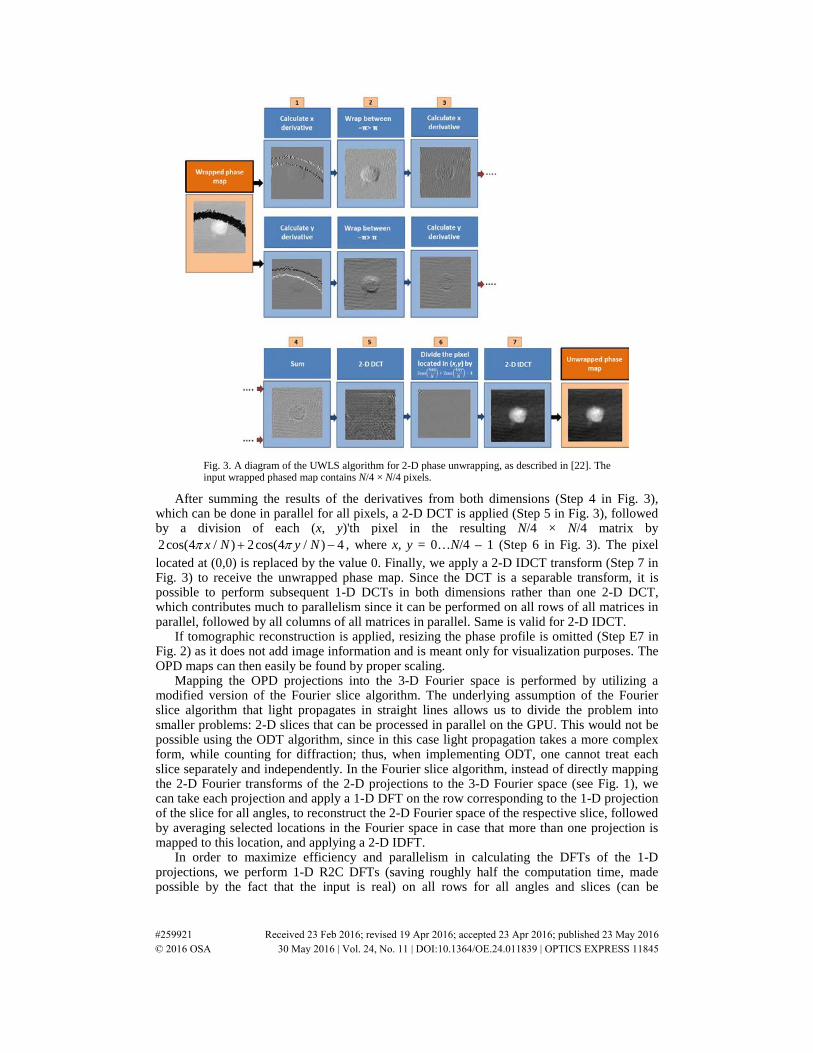
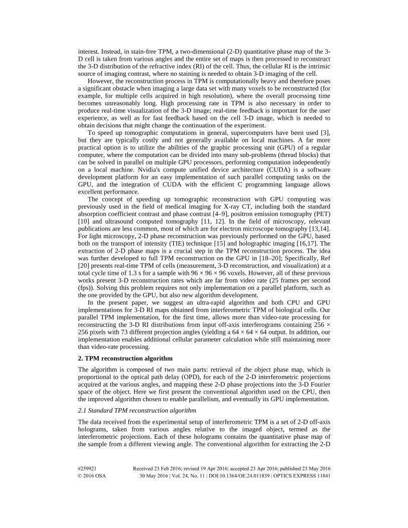
Fig. 3. A diagram of the UWLS algorithm for 2-D phase unwrapping, as described in [22]. The input wrapped phased map contains N/4 × N/4 pixels.

After summing the results of the derivatives from both dimensions (Step 4 in Fig. 3), which can be done in parallel for all pixels, a 2-D DCT is applied (Step 5 in Fig. 3), followed by a division of each (x, y)'th pixel in the resulting N/4 × N/4 matrix by 2cos(4 / ) 2cos(4 / ) 4x N y Nπ π+ − , where x, y = 0…N/4 – 1 (Step 6 in Fig. 3). The pixel located at (0,0) is replaced by the value 0. Finally, we apply a 2-D IDCT transform (Step 7 in Fig. 3) to receive the unwrapped phase map. Since the DCT is a separable transform, it is possible to perform subsequent 1-D DCTs in both dimensions rather than one 2-D DCT, which contributes much to parallelism since it can be performed on all rows of all matrices in parallel, followed by all columns of all matrices in parallel. Same is valid for 2-D IDCT.

If tomographic reconstruction is applied, resizing the phase profile is omitted (Step E7 in Fig. 2) as it does not add image information and is meant only for visualization purposes. The OPD maps can then easily be found by proper scaling.

Mapping the OPD projections into the 3-D Fourier space is performed by utilizing a modified version of the Fourier slice algorithm. The underlying assumption of the Fourier slice algorithm that light propagates in straight lines allows us to divide the problem into smaller problems: 2-D slices that can be processed in parallel on the GPU. This would not be possible using the ODT algorithm, since in this case light propagation takes a more complex form, while counting for diffraction; thus, when implementing ODT, one cannot treat each slice separately and independently. In the Fourier slice algorithm, instead of directly mapping the 2-D Fourier transforms of the 2-D projections to the 3-D Fourier space (see Fig. 1), we can take each projection and apply a 1-D DFT on the row corresponding to the 1-D projection of the slice for all angles, to reconstruct the 2-D Fourier space of the respective slice, followed by averaging selected locations in the Fourier space in case that more than one projection is mapped to this location, and applying a 2-D IDFT.

In order to maximize efficiency and parallelism in calculating the DFTs of the 1-D projections, we perform 1-D R2C DFTs (saving roughly half the computation time, made possible by the fact that the input is real) on all rows for all angles and slices (can be


implemented in parallel). When mapping the 2-D Fourier spaces of the various slices, we again use the Hermitian symmetry principle, which is useful here since only slightly more than half the Fourier space needs to be mapped in order to reconstruct the full slice in the image space (namely the non-redundant half of the Fourier space). This is done in the parallel implementation by having all pixels add their value to the corresponding location in the Fourier space in parallel, according to the specific row and the OPD map corresponding to the specific slice and angle, given that the location is in the non-redundant part of the Fourier space. After averaging the resultant Fourier space for all voxels in parallel, based on the number of projections added to each of the voxels (since more than one projection may be mapped to the same location), we perform N/4 2-D C2R IDFTs, once for each slice, in order to restore the 3-D distribution of the difference between the RI inside the object and in the medium. Finally, in order to restore the 3-D distribution of the RI of the object, the constant value of the RI of the medium can be added voxel-wise.

2.3 Implementation of the parallel algorithm on the GPU

Figure 4 illustrates the implementation of the proposed algorithm on the GPU. As shown in Fig. 4(a), prior to the reconstruction process, there is an offline initialization step performed once for every experimental setup. This step includes an offline processing of a single sample-free hologram, for beam referencing, and extraction of the location of the C.C. term, as explained in the previous section. The location matrix in the 2-D Fourier space used for the TPM processing, specifying where to map each projection in the 2-D cartesian grid as a function of the angle of the mapped projection, can also be computed offline as a part of the initialization step, since it is identical for all slices and reconstructions, for a constant number of projections. This information is then transferred to the GPU together with the experimental setup constants, such as the illumination wavelength, the pixel size of the camera, and the optical magnification (used for the DFTs, see [31]). In the GPU, proper space allocations are made, and plans for the various DFTs used in the algorithms are created using the CUDA FFT library (CuFFT), based on the proper number of projections and the input image size.

Fig. 4. A diagram of the GPU implementation of the parallel algorithm for TPM reconstruction: (a) The offline initialization step performed once for every hologram set. (b) Online reconstruction using the GPU.


After the one-time initialization process is completed, in the online reconstruction schematically illustrated in Fig. 4(b), a new set of interferometric projections is read by the CPU from the camera and transferred to the GPU. Then, all projections are processed in parallel to reconstruct the 3-D RI map of the imaged cell. Finally, the result is copied back to the CPU, where it is saved. This process is cyclic, repeated for every new set of interferometric projections, and since all variables can be overwritten, many TPM reconstruction cycles can be performed without special memory limitations. The timing of the full cycle of the algorithm includes reading to the CPU, memory transfer to the GPU, calculation on the GPU, memory transfer back to the CPU and saving on the CPU.

Up to the phase unwrapping stage, all steps described in the previous section can be implemented using CUDA with no special alterations. The hologram resampling (Step E1 in Fig. 2) can be done by considering each row in each of the resized images as a separate problem, or a thread block, where each thread performs the small task of calculating the value of the corresponding member in the row from the values it replaces according to Eq. (2). The subsequent 1-D R2C DFTs can be performed in parallel on all rows using the CuFFT library (which parallelizes the calculation of each transform as well). The C.C. term can then be extracted by using a number of blocks which is equal to the total number of rows in all holograms, where in each block each thread corresponds to one pixel in the cropped row, finding its value based on its known location in the block and the known location of the center of the C.C. term, which is found in the initialization step. After this step, the 1-D IDFTs can be performed in parallel for all rows using the CuFFT library, followed by extraction of the wrapped phase and beam referencing, both performed in parallel for all pixels, again by using a number of blocks equal to the total number of rows in all images, where in each block each thread corresponds to one pixel performing a simple calculation.

The phase unwrapping part requires several adjustments when implemented in CUDA. In the numeric derivative part, dividing the problem into sub-problems (thread-blocks) can be easily done for the x derivative by dividing to rows. Since the matrices are arranged in row-major order by default, such that rows are concatenated in the GPU memory and adjacent members in the same row (block) are also adjacent members in memory, this division allows efficient memory access, termed as good coalescing. For the y dimension, however, dividing the problem into thread blocks in the complementary form of columns would be bad practice, since adjacent rows are separated by a number of members equal to the number of columns in memory, making the global memory access highly inefficient, known as bad coalescing [32]. It is therefore better to find another approach for the y derivative. A simple strategy would be to simply transpose each matrix and apply the same process performed in the new x-direction. However, a more efficient strategy is to simply divide each image into rectangular tiles (where each tile is a thread block) instead of columns (where each column is a block) for calculating the y derivative, such that better coalescing is achieved in reading from global memory to shared memory in each tile. This, of course, comes with a price, since it forces the elements on the border to access global memory rather than shared memory, which is quicker, more than once; yet overall, it is the better alternative. In either setup of blocks, each thread corresponds to a single pixel, and all threads in the block use memory shared by the entire block to calculate the derivative, saving redundant time-consuming accesses to global memory, since in the numeric derivative calculation there is an overlap in the information used by each two neighboring pixels. Wrapping the derivatives (Step 2 in Fig. 3) can be done in parallel for all threads in the respective blocks used for the appropriate numeric derivative (x or y), as each of the threads corresponds to a single pixel. The parallel computation of the x and y derivatives can be implemented using streams, allowing the different kernels for the x and y derivatives to run simultaneously if free processors are available. It should however be noted, that the parallel calculation of the x and y derivatives is limited only to the first derivative in the y dimension, since the special tile-based implementation for the y dimension mandates separate kernels for the first and second derivative. This is due to the fact that there is use of information present outside of the tile for boundary elements, requiring that all blocks performing the first derivatives are done before starting the second derivative, and that


different blocks cannot be synchronized without terminating the kernel. The two x derivatives and wrappings can therefore be performed within one kernel in parallel to calculating the wrapped first derivative in y, while the kernel performing the second derivative in y can include the summation of the two matrices (Step 4 in Fig. 3).

The implementation of the 1-D DCTs and IDCTs in CUDA was based on the CuFFT library and the DCT-FFT relations given in [33], which can be implemented pixel-wise in a straightforward manner. In the 1-D DCT, a R2C DFT can be used for a more efficient calculation, and similarly in the 1-D IDCT, a C2R IDFT can be used. Note that another problem arises here with operations performed in the columns dimension due to the row-major format in the CuFFT library, which we solved by performing transpose on each matrix separately (such that in practice we arranged the original columns in row-major order). In order to save resources, the second part of the phase unwrapping algorithm can be modified to first perform a 1-D DCT on the rows, then transpose the resultant image, perform a 1-D DCT on the new rows, divide each pixel by the appropriate value as specified in Step 6 in Fig. 3, perform a 1-D IDCT on the rows, transpose the result, and perform the final 1-D IDCT on the new rows. This is equivalent to the process shown in Steps 5-7 in Fig. 3, since this transform is separable (therefore the order of rows/columns execution is irrelevant). The transpose function can also be time consuming and is best implemented here by dividing each transpose problem into rectangular thread-blocks to achieve better coalescing [34].

After extracting the unwrapped phase, calculating the OPD maps can be done in parallel in a straightforward manner, followed by performing 1-D R2C DFTs in parallel for all rows in all OPD maps with the CuFFT library. Before mapping the results to the respective 2-D Fourier spaces, all Fourier spaces must be initialized, as can be done efficiently using the cudaMemset function. Mapping each Fourier space can then be done as explained in the previous section, where every 1-D projection corresponds to a thread block, and each of its members corresponds to a thread, adding its value to the relevant location in the appropriate 2-D Fourier space respective of its row, given that it is mapped to the non-redundant part of the Fourier space. In order to apply this addition, we had to prevent a race condition in the multiple simultaneous reads and writes to memory, which occurs often since in many cases several values are mapped into the same pixel. All additions in those steps are therefore done using atomic add operations, meant to prevent race conditions by locking the memory slot until the read-increment-write operation is done. Though atomic operations are known as inefficient, the overall run time of the corresponding function relative to other more complicated options of implementation is still better. It is also useful to keep an accessory 2-D space for each 2-D Fourier space, used to count the number of projections added to each pixel (again, using an atomic add operation) for averaging purposes. Once the parallel, pixel-wise averaging is completed, 2-D C2R DFTs can be performed in parallel for all slices using the CuFFT library, to reconstruct the 3-D distribution of the RI of the imaged object.

3. Simulation results

We conducted interferometric tomography simulations based on a known RI distribution of a 3-D test target typically used for tomography, enabling the quantification of the reconstruction precision. The simulations imitated an off-axis interferometric system, where light was assumed to travel in straight lines.

For the first simulation, meant to compare the reconstruction quality of different algorithms implemented on different platforms, the input was 73 simulative off-axis image holograms, containing 256 × 256-pixels each, and taken in equal increments over a 180° range. For comparison, we implemented the following algorithms: (a) the standard algorithm on the CPU using Matlab, employing algorithm ‘A’ for phase extraction and the slice-version of the Fourier slice algorithm; (b) the sequential efficient algorithm (specified in Section 2.2, utilizing R2C and C2R transforms when applicable with the FFTW library) on the CPU using C programming language; and (c) the parallel efficient algorithm for the GPU using CUDA C on the GPU (specified in Section 2.3). The reconstruction results are presented in Fig. 5.


Fig. 5. A comparison between the reconstruction results obtained for simulation data for various reconstruction implementations. (a) A schematic model of the input object. (b–e) axial slice, (f–i) coronal slice, (j–m) sagittal slice. Images (b), (f), and (j) are the true (input) RI distribution. Images (c), (g), and (k) are the results for the standard CPU reconstruction in Matlab. Images (d), (h), and (l) are the results for the efficient CPU implementation in C. Images (e), (i), and (m) are the results for the efficient GPU implementation with CUDA C. Colorbar represents RI values.

The error in reconstruction was calculated for each implementation as the mean squared error (MSE) relative to the true distribution, and was 4.9179×10˗6 for the Matlab implementation and 3.7551×10˗5 for both the CPU/C and GPU/CUDA C implementations. In order to make this comparison, as well as for visualization purposes, we resampled both the true RI distribution and the result of the Matlab implementation four times in each dimension to a size of 64 × 64 × 64, so that they would be comparable to the results received by the efficient algorithms implemented in CPU/C and GPU/CUDA C.

Fig. 6. The dependency of the 3-D RI reconstruction quality in the resolution of the input holograms (a) A schematic model of the input object. (b–d) axial slice, (e–g) coronal slice, (h-j) sagittal slice. Images (b), (e), and (h) are the reconstruction results for a 256 × 256 hologram set input, images (c), (f), and (i) are for the 512 × 512 hologram set input and images (d), (g), and (j) are for the 1024 × 1024 hologram set input. Colorbar represents RI values.


For the second simulation, meant to compare the reconstruction quality for input holograms of different resolutions, the input was 73 simulative off-axis image holograms, containing either 256 × 256, 512 × 512 or 1024 × 1024-pixels each, and taken in equal increments over a 180° range. All reconstructions were implemented using the parallel efficient algorithm for the GPU using CUDA C on the GPU. The reconstruction results are presented in Fig. 6. As can be seen from the results in Figs. 6(b)–6(j), an increase in the quality of reconstruction is visible with the increase in resolution, yet it is most prominent in the transition from 256 × 256 holograms (Figs. 6(b), 6(e), and 6(h)) to 512 × 512 holograms (Figs. 6(c), 6(f), and 6(i)), as the size of the feature is too small to be properly imaged with such resolution.

4. Experimental results

4.1 Experimental setup

For data acquisition, we used single-cell rotation by micro-manipulation, while recording off-axis image holograms. Figure 7(a) shows a schematic of the experimental system used. Light from a helium-neon laser is reflected to the sample by mirror M1 and then magnified by a 60 × immersion-oil microscope objective. The enlarged image is projected by tube lens TL onto the exit of the microscope, where an external off-axis interferometric module is positioned [35,36]. In this module, the magnified sample beam is split using beam splitter BS. One of the beams is spatially filtered using lenses L1 and L2 and pinhole P that effectively creates a reference beam that does not contain spatial modulation from the sample. The other beam from BS is projected through retro-reflector RR at a small angle, and together with the reference beam creates an off-axis hologram on the camera. We acquired interferometric projections of T-cells isolated from blood. The resulting mid-sagittal, mid-coronal and mid-axial sections of the reconstructed 3-D RI profile using the efficient GPU implementation are shown in Figs. 7(b)-7(d). Figures 7(e)-7(g) present the data as reconstructed with the conventional, time-consuming 'Algorithm A' for phase extraction and the ODT algorithm for tomographic reconstruction, as implemented in Matlab. As can be seen, these results are similar to the ones achieved using the efficient implementation presented in this paper.

Fig. 7. (a) Optical setup scheme for interferometric TPM with rotation of single cells. The system combines cell micro-manipulation for cell rotation and an external interferometric module for acquisition of off-axis holograms during cell rotation. MO: Microscope objective; S: sample; TL: Tube lens; M1˗M3: Mirrors; L1, L2: Lenses in 4f configuration; BS: Beam splitter; RR: Retro-reflector; P: Pinhole. (b-g) The reconstructed 3-D RI map of a T-cell suspended in a medium, as acquired with the experimental setup. The input for the reconstruction was 73 off-axis holograms taken in equal angular increments over a 180° range, each of which in the size of 256 × 256 pixels. Colorbar represents RI values, where 1.33 is the RI of the medium. (b-d) Reconstruction results using the efficient algorithm presented in Section 2 implemented in C language on the GPU. (b) Mid-sagittal slice; (c) Mid-coronal slice; (d) Mid-axial slice; (e-g) The coinciding cases for (b-d), but when implementing the conventional phase extraction and ODT in Matlab. These results show minimal loss of accuracy when implementing the proposed efficient algorithms.


4.2 Reconstruction timing

All computations were performed on a desktop computer equipped with Intel's core i7-5960X 3.00 GHz 64.0 GB RAM 64 bit CPU, and a Tesla K20c GPU. We implemented and compared three cases, the proposed GPU implementation using C, the proposed CPU implementation using C, and the conventional (slow) CPU implementation using Matlab. For the GPU, we implemented the algorithm described in Section 2.3, where the programming environment was Visual Studio 2013 and Nvidia's CUDA C. We used a 64-bit project and single floating-point precision. Timing was done using the Nvidia visual profiler. To have a fair comparison to the CPU, we implemented the equivalent sequential algorithm, still using the efficient algorithms specified in Section 2.2, utilizing R2C and C2R transforms when applicable with the FFTW library. The computation was performed on a 64-bit project with single floating point precision in Visual Studio 2013 with C programming language. Timing was done using the Windows QueryPerformanceCounter function. We also implemented the standard algorithm on the CPU, employing algorithm ‘A’ for phase extraction and the slice-version of the Fourier slice algorithm similar to the one used for the parallel algorithm, using MatlabR2015b with double precision. Timing was done using the Matlab “Tic-Toc” function. The presented run times include the calculation time, as well as memory transfers to and from the GPU, when relevant, but do not include the one-time initialization step.

We first compared the three algorithm for simulative input data (see Section 3) of 73 projections taken in equal increments over a 180° range for a 256 × 256 input (not including reading and writing to/from the CPU). The standard Matlab implementation run time was 8.452 s, the efficient C implementation was 0.1 s, and the efficient CUDA C implementation was 0.007 s, illustrating the large gain obtained by using the proposed algorithms.

To further evaluate the increase in the reconstruction rate obtained by the proposed method, we performed tomographic reconstruction for input holograms of 256 × 256, 512 × 512 and 1024 × 1024 pixels, all with 73 projections taken while rotating over 180° in equal increments, comparing the efficient C/CPU implementation to the CUDA C/GPU implementation. The results are presented in Fig. 8 (in terms of reconstruction rate, in fps) and Table 1 (in terms of timing in ms).

Figure 8 shows two different comparisons of reconstruction rates between the CPU and GPU for various sizes of input holograms: when we include reading and writing to/from the CPU (Fig. 8(a)), and when we do not include them (Fig. 8(b)).

Fig. 8. Average reconstruction rates (fps) and speedups when comparing the CPU and GPU efficient implementations, for various input hologram sizes (a) Rates including reading and writing to/from the CPU and memory transfers to/from the GPU when relevant; (b) Rates not including reading and writing to/from the CPU.


As can be seen in Fig. 8(b), even though the GPU timing included memory transfers that did not exist for the CPU implementation, the speedup obtained by the GPU is substantial, reaching an improvement of 24 × for 1 Megapixel input holograms, when not including reading and writing (Fig. 8(b)), which is identical in both implementations. When including the time consumed by reading and writing to the CPU (Fig. 8(a)), we were still able to reach a rate of 67.52 3-D reconstructions per second using the GPU for 256 × 256 pixels inputs with 73 projection angles (yielding 64 × 64 × 64 voxels outputs); still much higher than video rate.

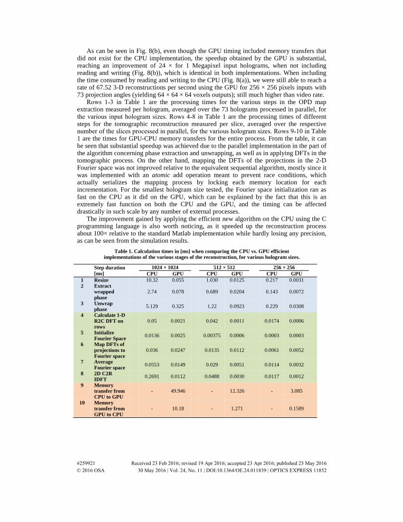
Rows 1˗3 in Table 1 are the processing times for the various steps in the OPD map extraction measured per hologram, averaged over the 73 holograms processed in parallel, for the various input hologram sizes. Rows 4˗8 in Table 1 are the processing times of different steps for the tomographic reconstruction measured per slice, averaged over the respective number of the slices processed in parallel, for the various hologram sizes. Rows 9˗10 in Table 1 are the times for GPU-CPU memory transfers for the entire process. From the table, it can be seen that substantial speedup was achieved due to the parallel implementation in the part of the algorithm concerning phase extraction and unwrapping, as well as in applying DFTs in the tomographic process. On the other hand, mapping the DFTs of the projections in the 2-D Fourier space was not improved relative to the equivalent sequential algorithm, mostly since it was implemented with an atomic add operation meant to prevent race conditions, which actually serializes the mapping process by locking each memory location for each incrementation. For the smallest hologram size tested, the Fourier space initialization ran as fast on the CPU as it did on the GPU, which can be explained by the fact that this is an extremely fast function on both the CPU and the GPU, and the timing can be affected drastically in such scale by any number of external processes.

The improvement gained by applying the efficient new algorithm on the CPU using the C programming language is also worth noticing, as it speeded up the reconstruction process about 100× relative to the standard Matlab implementation while hardly losing any precision, as can be seen from the simulation results.

Table 1. Calculation times in [ms] when comparing the CPU vs. GPU efficient implementations of the various stages of the reconstruction, for various hologram sizes.

Step duration [ms]

1024 × 1024 512 × 512 256 × 256 CPU GPU CPU GPU CPU GPU 1 Resize 10.32 0.055 1.030 0.0125 0.217 0.0031 2 Extract

wrapped phase

2.74 0.078 0.689 0.0204 0.143 0.0072

3 Unwrap phase

5.129 0.325 1.22 0.0923 0.229 0.0308

4 Calculate 1-D R2C DFT on rows

0.05 0.0021 0.042 0.0011 0.0174 0.0006

5 Initialize Fourier Space

0.0136 0.0025 0.00375 0.0006 0.0003 0.0003

6 Map DFTs of projections to Fourier space

0.036 0.0247 0.0135 0.0112 0.0061 0.0052

7 Average Fourier space

0.0553 0.0149 0.029 0.0051 0.0114 0.0032

8 2D C2R IDFT

0.2691 0.0112 0.0488 0.0030 0.0117 0.0012

9 Memory transfer from CPU to GPU

- 49.946 - 12.326 - 3.085

10 Memory transfer from GPU to CPU

- 10.18 - 1.271 - 0.1589


4.3 Calculating cellular parameters

Since the new implementation enables processing rates far higher than video rate for reconstructions obtained from input holograms of 256 × 256 pixels, we were able to perform further calculations to extract various quantitative parameters from the 3-D distribution, while still maintaining higher than video-rate calculation. The 3-D RI distribution of a cell provides quantitative morphological and biochemical information, including the cellular dry mass, volume, surface area, and sphericity, and allows separation of heterogeneous populations as was demonstrated for white blood cells [37], which could be valuable for label-free cell sorting following a blood test. This application would also require fast processing capabilities. We obtained the cellular volume by counting the number of voxels inside the cell 3-D RI map multiplied by the voxel size. This was implemented in CUDA using a threshold value differentiating the object from the medium and an atomic add operation. The average value of the RI of the cytoplasm was also calculated, by summing the values of the RIs in the appropriate range with an atomic add operation and dividing the result with the number of voxels. The surface area was calculated by counting the number of boundary voxels in the binary image obtained from the volume threshold, and was implemented using morphological operations in cubic parallel thread blocks and the atomic add operation. Based on these measurements, the sphericity, dry mass and dry mass density can be calculated in a straightforward manner [37].

We were able to deduce various cellular parameters in video rate for reconstructions obtained from input holograms of 256 × 256 pixels with 73 different projection angles. The cell volume was calculated as 169 fL, its surface area as 183 µm2, its average cytoplasm RI as 1.364, its sphericity as 0.8, its dry mass density as 17.45 g/dL, and its dry mass as 29.54 pg. Performing these additional calculations cost less than 30% of the 3-D reconstruction time, still enabling much higher than video rate for the full process.

5. Discussion and conclusions

The parallel algorithm for rapid TPM processing presented in this paper requires the dimensions of the data as well as the number of projections and parameters of the experimental setup to be known at the initialization part and remain constant for all iterations. This requirement, while being somewhat restricting in its demand for a constant setup, allows for an unlimited number of iterations from the memory point of view. In our implementation, we assumed that each input hologram is square, where each of its dimensions must be a power of 2 which is not greater than 1024 × 1024 (since each row is processed as a thread block where each member is respective of a thread, and the CUDA architecture is limited by 1024 threads per block). The demand for a power of 2 dimension also increases efficiency, as it allows execution in units that are multiplications of 32, which is the number of threads that can be executed simultaneously on the same processor. The algorithm also assumes that the input from the imaging system is a set of off-axis holograms taken at equal rotation increments over a 180° range with a wide illumination beam covering the entire sample, as well as that the rotation axis is constant and centered for all projections. In case of transverse axial or axial rotation errors, digital centering of mass [26] and holographic 3D tracking [38] must be used, which might increase the computation complexity. It is also assumed that quality of acquisition is such that no illumination slope is present, that the object is static during acquisition, and that no pre-filtering of the phase maps is required due to noise.

In this implementation, we chose to use the Fourier slice algorithm for the tomographic reconstruction, which neglects diffraction, rather than the more accurate but less parallelizable ODT algorithm. We do not claim to compete with the reconstruction quality of ODT, but rather to give a good approximation, as experimentally verified, in an unprecedented time.

To further increase computation rate and allow video-rate computation for larger inputs, fewer projections can be taken per reconstruction. For example, in this paper all timings were made for a rotation increment of 2.5°; however, if a 5° increment was used, roughly half the projections would be processed and the processing time would decrease substantially, but at


the price of reconstruction quality. The trade-off between reconstruction quality and processing time as a function of the rotation increment for large inputs must therefore be considered individually, according to the application and its specific requirements.

Finally, our implementation assumes that all input projections for one sample instance (e.g. 73 projections in our experiments) are already acquired at the time of computation, so a proper experimental setup must be developed in order to acquire the holograms in rates high enough to allow the full process, including both acquisition and computation, to reach a rate of 25 reconstructions per second, where the exact rate needed for the acquisition depends on the computation rate. In our experiments, we used micro-manipulation on a single cell to rotate the cell and acquired the projections within 12 s. A faster method for TPM cell capturing is the rotation of the illumination angle using a rapid scanning mirror (e.g., [20]).

In conclusion, we presented a new parallel algorithm that enables a significant speedup in the processing times of TPM. For the first time, we obtained more than video rate processing times for 256 × 256 pixel input off-axis holograms with 73 different projection angles, which enables the calculation of additional cellular parameters, while still maintaining video-rate processing. We foresee that the proposed algorithm will be used for real-time label-free 3-D visualization, control and sorting of live cells in medical applications and biological research.

Acknowledgments

This research was supported by the TAU-Berkeley Raymond and Beverly Sackler Fund for Convergence Research. We thank Dr. Ksawery Kalinowski from the OMNI group in Tel Aviv University for useful remarks.


video-rate processing in tomographic phase microscopy …omni/cuda_tpm_oe2016.pdf · video-rate...

Documents