helpgecmit.files.wordpress.com · web viewaim : create an .arff file for following attributes and...

Data Mining and Business Intelligence (2170715) Enrollment No: 130160116019

EXPERIMENT-1

Aim :- Write programs to perform Equal Frequency Binning.

#include<stdio.h>int main(){

int data[9],old[9];int x,y;int i,j,sum=0,avg=0;

printf("\nProgram for equal frequency binning");printf("\n------------------------------------------\n");

printf("\nEnter data:-\n");for(i=0;i<9;i++){

printf("Data %d :- ",i+1);scanf("%d",&data[i]);old[i]=data[i];

}

for(j=0;j<9;j+=3){

sum=0;for(i=0;i<3;i++){

sum+=data[i+j];}avg=sum/3;for(i=0;i<3;i++){

data[i+j]=avg;}//printf("\nAvg:- %d",sum/3);

}

printf("\nData after binning using mean:-");

for(i=0;i<9;i++){

printf("\ndata %d :- %d",i+1,data[i]);}

for(i=0;i<9;i++){

data[i]=old[i];}

for(i=0;i<9;i+=3)

GECM (BE IT-SEM-VII) 1


{

x=data[i+1]-data[i];y=data[i+2]-data[i+1];if(x<y){

data[i+1]=data[i];}else if(x>y){

data[i+1]=data[i+2];}else{

data[i+1]=data[i];}

}

printf("\nData after binning using bounding:-");

for(i=0;i<9;i++){

printf("\ndata %d :- %d",i+1,data[i]);}

}Output:



EXPERIMENT-2

Aim :- Write programs to perform the following tasks:

a) Min max normalization

b) Z score normalization

c) Decimal scaling

#include<stdio.h>

#define n 5

int main()

{

int i,j;

float num[10];

float min,max,v,newmin,newmax;

float vd,mean,divider,dev;

printf("\nProgram for transformation techniques");

printf("\n------------------------------------------\n");

for(i=0;i<n;i++)

{

printf("\nEnter value of num %d :-",i+1);

scanf("%f",&num[i]);

}

min=35000;

max=0;

for(i=0;i<(n-1);i++)

{

if(num[i]<num[i+1])

{



min=(min<num[i])?min:num[i];

max=(max>num[i+1])?max:num[i+1];

}

else

{ min=(min<num[i+1])?min:num[i+1];

max=(max>num[i])?max:num[i];

}

}

printf("\nMin :- %f",min);

printf("\nMax :- %f",max);

printf("\n\nEnter value to be normalized(v) :-");

scanf("%f",&v);

printf("\n\n\nMIN-MAX NORMALIZATION:-");

printf("\n----------------------------------");

printf("\nEnter value of new min :-");

scanf("%f",&newmin);

printf("\nEnter value of new max :-");

scanf("%f",&newmax);

vd=(v-min)*(newmax-newmin)/(max-min)+newmin;

printf("\nNORMALISED VALUE(v') :- %f",vd);

printf("\n\n\nZ-SCORE NORMALIZATION:-");

printf("\n----------------------------------");

printf("\nEnter value of mean :-");

scanf("%f",&mean);

printf("\nEnter value of deviation :-");

scanf("%f",&dev);

vd=(v-mean)/dev;



printf("\nNORMALIZED VALUE(v') :- %f",vd);

printf("\n\n\nNORMALIZATION BY DECIMAL SCALING:-");

printf("\n----------------------------------");

i=0;

while(!(max>0 && max<1))

{

max=max/10;

i++;

}

divider=1;

for(j=0;j<i;j++)

{

divider=10*divider;

}

printf("\nDIVIDER :- %f",divider);

printf("\n\nNORMALIZED VALUES OF ITEMS :-");

for(i=0;i<n;i++)

{

printf("\nNum %d :- %f",i+1,(num[i]/divider));

}

}



Output:



EXPERIMENT-3

Aim :- Overview of SQL Server 2005 Databases and analysis services.

Software Required: Analysis services- SQL Server-2005.

Knowledge Required: Data Mining Concepts

Theory/Logic:

� Data Mining

¾ Act of excavation in the data from which patterns can be extracted

¾ Alternative name: Knowledge discovery in databases (KDD)

¾ Multiple disciplines: database, statistics, artificial intelligence

¾ Fastly maturing technology ¾ Unlimited applicability

Data Mining Tasks - Summary

� Classification ƒ Regression

� Segmentation

� Association Analysis

� Anomaly detection � Sequence Analysis

� Time-series Analysis

� Text categorization


Figure 1 D: ata mining process

Data Mining Management System

(DMMS)

Mining Model

Define a model

Train the model Training Data

Test Data Test the model

Prediction u

sing the model

Prediction Input Data


� Advanced insights discovery

� Others

The data mining tutorial is designed to walk you through the process of creating data mining models in Microsoft SQL Server 2005. The data mining algorithms and tools in SQL Server 2005 make it easy to build a comprehensive solution for a variety of projects, including market basket analysis, forecasting analysis, and targeted mailing analysis. The scenarios for these solutions are explained in greater detail later in the tutorial.

The most visible components in SQL Server 2005 are the workspaces that you use to create and work with data mining models. The online analytical processing (OLAP) and data mining tools are consolidated into two working environments: Business Intelligence Development Studio and SQL Server Management Studio. Using Business Intelligence Development Studio, you can develop an Analysis Services project disconnected from the server. When the project is ready, you can deploy it to the server. You can also work directly against the server. The main function of SQL Server Management Studio is to manage the server. Each environment is described in more detail later in this introduction.

All of the data mining tools exist in the data mining editor. Using the editor you can manage mining models, create new models, view models, compare models, and create predictions based on existing models.

After you build a mining model, you will want to explore it, looking for interesting patterns and rules. Each mining model viewer in the editor is customized to explore models built with a specific algorithm.

Often your project will contain several mining models, so before you can use a model to create predictions, you need to be able to determine which model is the most accurate. For this reason, the editor contains a model comparison tool called the Mining Accuracy Chart tab. Using this tool you can compare the predictive accuracy of your models and determine the best model.

To create predictions, you will use the Data Mining Extensions (DMX) language. DMX extends SQL, containing commands to create, modify, and predict against mining models. Because creating a prediction can be complicated, the data mining editor contains a tool called Prediction Query Builder, which allows you to build queries using a graphical interface. You can also view the DMX code that is generated by the query builder.

The key to creating a mining model is the data mining algorithm. The algorithm finds patterns in the data that you pass it, and it translates them into a mining model — it is the engine behind the process. SQL Server 2005 includes nine algorithms:

1. Microsoft Decision Trees

2. Microsoft Clustering

3. Microsoft Naïve Bayes

4. Microsoft Sequence Clustering

5. Microsoft Time Series

6. Microsoft Association



7. Microsoft Neural Network

8. Microsoft Linear Regression

9. Microsoft Logistic Regression

Using a combination of these nine algorithms, you can create solutions to common business problems. Some of the most important steps in creating a data mining solution are consolidating, cleaning, and preparing the data to be used to create the mining models. SQL Server 2005 includes the Data Transformation Services (DTS) working environment, which contains tools that you can use to clean, validate, and prepare your data. The audience for this tutorial is business analysts, developers, and database administrators who have used data mining tools before and are familiar with data mining concepts.

Business Intelligence Development Studio

Business Intelligence Development Studio is a set of tools designed for creating business intelligence projects. Because Business Intelligence Development Studio was created as an IDE environment in which you can create a complete solution, you work disconnected from the server. You can change your data mining objects as much as you want, but the changes are not reflected on the server until after you deploy the project.

Working in an IDE is beneficial for the following reasons:

• You have powerful customization tools available to configure Business Intelligence Development Studio to suit your needs.

• You can integrate your Analysis Services project with a variety of other business intelligence projects encapsulating your entire solution into a single view.

• Full source control integration enables your entire team to collaborate in creating a complete business intelligence solution.

The Analysis Services project is the entry point for a business intelligence solution. An Analysis Services project encapsulates mining models and OLAP cubes, along with supplemental objects that make up the Analysis Services database. From Business Intelligence Development Studio, you can create and edit Analysis Services objects within a project and deploy the project to the appropriate Analysis Services server or servers.

Working with Data Mining

Data mining gives you access to the information that you need to make intelligent decisions about difficult business problems. Microsoft SQL Server 2005 Analysis Services (SSAS) provides tools for data mining with which you can identify rules and patterns in your data, so that you can determine why things happen and predict what will happen in the future. When you create a data mining solution in Analysis Services, you first create a model that describes your business problem, and then you run your data through an algorithm that generates a mathematical model of the data, a process that is known as training the model. You can then either visually explore the mining model or create prediction queries against it. Analysis Services can use datasets from both relational and OLAP databases, and includes a variety of algorithms that you can use to investigate that data.



SQL Server 2005 provides different environments and tools that you can use for data mining. The following sections outline a typical process for creating a data mining solution, and identify the resources to use for each step.

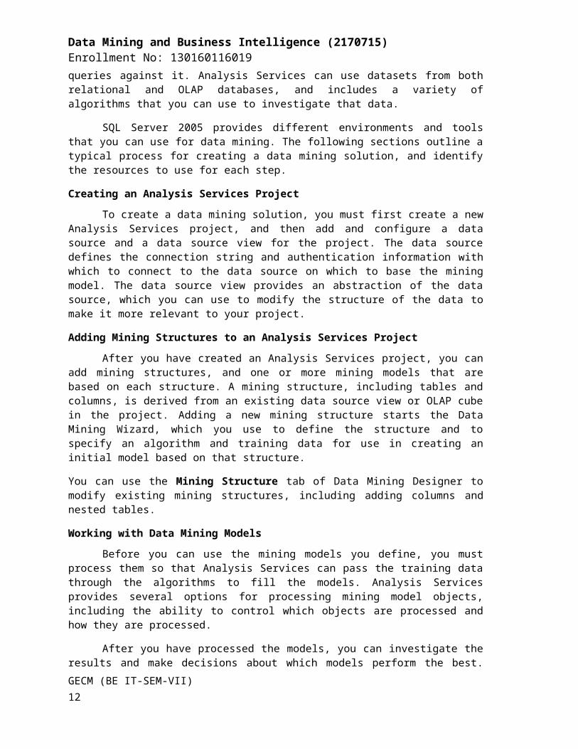
Creating an Analysis Services Project

To create a data mining solution, you must first create a new Analysis Services project, and then add and configure a data source and a data source view for the project. The data source defines the connection string and authentication information with which to connect to the data source on which to base the mining model. The data source view provides an abstraction of the data source, which you can use to modify the structure of the data to make it more relevant to your project.

Adding Mining Structures to an Analysis Services Project

After you have created an Analysis Services project, you can add mining structures, and one or more mining models that are based on each structure. A mining structure, including tables and columns, is derived from an existing data source view or OLAP cube in the project. Adding a new mining structure starts the Data Mining Wizard, which you use to define the structure and to specify an algorithm and training data for use in creating an initial model based on that structure.

You can use the Mining Structure tab of Data Mining Designer to modify existing mining structures, including adding columns and nested tables.

Working with Data Mining Models

Before you can use the mining models you define, you must process them so that Analysis Services can pass the training data through the algorithms to fill the models. Analysis Services provides several options for processing mining model objects, including the ability to control which objects are processed and how they are processed.

After you have processed the models, you can investigate the results and make decisions about which models perform the best. Analysis Services provides viewers for each mining model type, within the Mining Model Viewer tab in Data Mining Designer, which you can use to explore the mining models. Analysis Services also provides tools, in the Mining Accuracy Chart tab of the designer, that you can use to directly compare mining models and to choose the mining model that works best for your purpose. These tools include a lift chart, a profit chart, and a classification matrix.

Creating Predictions

The main goal of most data mining projects is to use a mining model to create predictions. After you explore and compare mining models, you can use one of several tools to create predictions. Analysis Services provides a query language called Data Mining Extensions (DMX) that is the basis for creating predictions. To help you build DMX prediction queries, SQL Server provides a query builder, available in SQL Server Management Studio and Business Intelligence Development Studio, and DMX templates for the query editor in Management Studio. Within BI Development Studio, you access the query builder from the Mining Model Prediction tab of Data Mining Designer.

SQL Server Management Studio

After you have used BI Development Studio to build mining models for your data mining project, you can manage and work with the models and create predictions in Management Studio.



SQL Server Reporting Services

After you create a mining model, you may want to distribute the results to a wider audience. You can use Report Designer in Microsoft SQL Server 2005 Reporting Services (SSRS) to create reports, which you can use to present the information that a mining model contains. You can use the result of any DMX query as the basis of a report, and can take advantage of the parameterization and formatting features that are available in Reporting Services.

Working Programmatically with Data Mining

Analysis Services provides several tools that you can use to programmatically work with data mining. The Data Mining Extensions (DMX) language provides statements that you can use to create, train, and use data mining models. You can also perform these tasks by using a combination of XML for Analysis (XMLA) and Analysis Services Scripting Language (ASSL), or by using Analysis Management Objects (AMO). You can access all the metadata that is associated with data mining by using data mining schema rowsets. For example, you can use schema rowsets to determine the data types that an algorithm supports, or the model names that exist in a database.

Data Mining Concepts

Data mining is frequently described as "the process of extracting valid, authentic, and actionable information from large databases." In other words, data mining derives patterns and trends that exist in data. These patterns and trends can be collected together and defined as a mining model. Mining models can be applied to specific business scenarios, such as:

• Forecasting sales.

• Targeting mailings toward specific customers.

• Determining which products are likely to be sold together.

• Finding sequences in the order that customers add products to a shopping cart.

An important concept is that building a mining model is part of a larger process that includes everything from defining the basic problem that the model will solve, to deploying the model into a working environment. This process can be defined by using the following six basic steps:

1. Defining the Problem

2. Preparing Data

3. Exploring Data

4. Building Models

5. Exploring and Validating Models

6. Deploying and Updating Models



The following diagram describes the relationships between each step in the process, and the technologies in Microsoft SQL Server 2005 that you can use to complete each step.

Although the process that is illustrated in the diagram is circular, each step does not necessarily lead directly to the next step. Creating a data mining model is a dynamic and iterative process. After you explore the data, you may find that the data is insufficient to create the appropriate mining models, and that you therefore have to look for more data. You may build several models and realize that they do not answer the problem posed when you defined the problem, and that you therefore must redefine the problem. You may have to update the models after they have been deployed because more data has become available. It is therefore important to understand that creating a data mining model is a process, and that each step in the process may be repeated as many times as needed to create a good model.

SQL Server 2005 provides an integrated environment for creating and working with data mining models, called Business Intelligence Development Studio. The environment includes data mining algorithms and tools that make it easy to build a comprehensive solution for a variety of projects.



Defining the Problem

The first step in the data mining process, as highlighted in the following diagram, is to clearly define the business problem.

This step includes analyzing business requirements, defining the scope of the problem, defining the metrics by which the model will be evaluated, and defining the final objective for the data mining project. These tasks translate into questions such as the following:

• What are you looking for?

• Which attribute of the dataset do you want to try to predict?

• What types of relationships are you trying to find?

• Do you want to make predictions from the data mining model or just look for interesting patterns and associations?

• How is the data distributed?

• How are the columns related, or if there are multiple tables, how are the tables related?

To answer these questions, you may have to conduct a data availability study, to investigate the needs of the business users with regard to the available data. If the data does not support the needs of the users, you may have to redefine the project.



Preparing Data

The second step in the data mining process, as highlighted in the following diagram, is to consolidate and clean the data that was identified in the Defining the Problem step.

Microsoft SQL Server 2005 Integration Services (SSIS) contains all the tools that you need to complete this step, including transforms to automate data cleaning and consolidation.

Data can be scattered across a company and stored in different formats, or may contain inconsistencies such as flawed or missing entries. For example, the data might show that a customer bought a product before that customer was actually even born, or that the customer shops regularly at a store located 2,000 miles from her home. Before you start to build models, you must fix these problems. Typically, you are working with a very large dataset and cannot look through every transaction. Therefore, you have to use some form of automation, such as in Integration Services, to explore the data and find the inconsistencies.

Exploring Data

The third step in the data mining process, as highlighted in the following diagram, is to explore the prepared data.



You must understand the data in order to make appropriate decisions when you create the models. Exploration techniques include calculating the minimum and maximum values, calculating mean and standard deviations, and looking at the distribution of the data. After you explore the data, you can decide if the dataset contains flawed data, and then you can devise a strategy for fixing the problems.

Data Source View Designer in BI Development Studio contains several tools that you can use to explore data.

Building Models

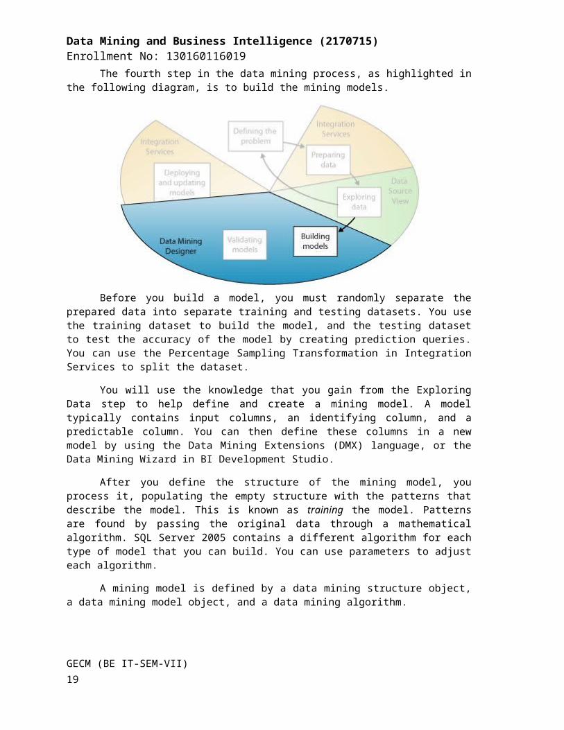
The fourth step in the data mining process, as highlighted in the following diagram, is to build the mining models.

Before you build a model, you must randomly separate the prepared data into separate training and testing datasets. You use the training dataset to build the model, and the testing dataset to test the accuracy of the model by creating prediction queries. You can use the Percentage Sampling Transformation in Integration Services to split the dataset.

You will use the knowledge that you gain from the Exploring Data step to help define and create a mining model. A model typically contains input columns, an identifying column, and a predictable column. You can then define these columns in a new model by using the Data Mining Extensions (DMX) language, or the Data Mining Wizard in BI Development Studio.

After you define the structure of the mining model, you process it, populating the empty structure with the patterns that describe the model. This is known as training the model. Patterns are found by passing the original data through a mathematical algorithm. SQL Server 2005 contains a different algorithm for each type of model that you can build. You can use parameters to adjust each algorithm.

A mining model is defined by a data mining structure object, a data mining model object, and a data mining algorithm.



Microsoft SQL Server 2005 Analysis Services (SSAS) includes the following algorithms:

• Microsoft Decision Trees Algorithm

• Microsoft Clustering Algorithm

• Microsoft Naive Bayes Algorithm

• Microsoft Association Algorithm

• Microsoft Sequence Clustering Algorithm

• Microsoft Time Series Algorithm

• Microsoft Neural Network Algorithm (SSAS)

• Microsoft Logistic Regression Algorithm

• Microsoft Linear Regression Algorithm

Exploring and Validating Models

The fifth step in the data mining process, as highlighted in the following diagram, is to explore the models that you have built and test their effectiveness.

You do not want to deploy a model into a production environment without first testing how well the model performs. Also, you may have created several models and will have to decide which model will perform the best. If none of the models that you created in the Building Models step perform well, you may have to return to a previous step in the process, either by redefining the problem or by reinvestigating the data in the original dataset.

You can explore the trends and patterns that the algorithms discover by using the viewers in Data Mining Designer in BI Development Studio. You can also test how well the models create predictions by using tools in the designer such as the lift chart and classification matrix. These tools require the testing data that you separated from the original dataset in the model-building step.



Deploying and Updating Models

The last step in the data mining process, as highlighted in the following diagram, is to deploy to a production environment the models that performed the best.

After the mining models exist in a production environment, you can perform many tasks, depending on your needs. Following are some of the tasks you can perform:

• Use the models to create predictions, which you can then use to make business decisions. SQL Server provides the DMX language that you can use to create prediction queries, and Prediction Query Builder to help you build the queries.

• Embed data mining functionality directly into an application. You can include Analysis Management Objects (AMO) or an assembly that contains a set of objects that your application can use to create, alter, process, and delete mining structures and mining models. Alternatively, you can send XML for Analysis (XMLA) messages directly to an instance of Analysis Services.

• Use Integration Services to create a package in which a mining model is used to intelligently separate incoming data into multiple tables. For example, if a database is continually updated with potential customers, you could use a mining model together with Integration Services to split the incoming data into customers who are likely to purchase a product and customers who are likely to not purchase a product.

Create a report that lets users directly query against an existing mining model. Updating the model is part of the deployment strategy. As more data comes into the organization, you must reprocess the models, thereby improving their effectiveness.



EXPERIMENT-4

Aim :- Design and Create cube by identifying measures and dimensions for Star Schema, Snowflake Schema.


Knowledge Required: Data cube

Theory/Logic:

Creating a Data Cube To build a new data cube using BIDS, you need to perform these steps:

• Create a new Analysis Services project

• Define a data source

• Define a data source view

• Invoke the Cube Wizard

We’ll look at each of these steps in turn.

Creating a New Analysis Services Project To create a new Analysis Services project, you use the New Project dialog box in BIDS.

This is very similar to creating any other type of new project in Visual Studio.

To create a new Analysis Services project, follow these steps:

1. Select Microsoft SQL Server 2005 ⇒SQL Server Business Intelligence. Development Studio from the Programs menu to launch Business Intelligence Development Studio.

2. Select File ⇒ New ⇒ Project.

3. In the New Project dialog box, select the Business Intelligence Projects project type.

4. Select the Analysis Services Project template.

5. Name the new project AdventureWorksCube1 and select a convenient location to save it.

6. Click OK to create the new project.



Figure 1 shows the Solution Explorer window of the new project, ready to be populated with objects

Figure 1: New Analysis Services project

Defining a Data Source To define a data source, you’ll use the Data Source Wizard. You can launch this wizard by right-clicking on the Data Sources folder in your new Analysis Services project. The wizard will walk you through the process of defining a data source for your cube, including choosing a connection and specifying security credentials to be used to connect to the data source.

To define a data source for the new cube, follow these steps:

1. Right-click on the Data Sources folder in Solution Explorer and select New Data Source.

2. Read the first page of the Data Source Wizard and click Next.

3. You can base a data source on a new or an existing connection. Because you don’t have any existing connections, click New.

4. In the Connection Manager dialog box, select the server containing your analysis services sample database from the Server Name combo box.

5. Fill in your authentication information.

6. Select the Native OLE DB\SQL Native Client provider (this is the default provider).

7. Select the AdventureWorksDW database. Figure 2 shows the filled-in Connection Manager dialog box.

8. Click OK to dismiss the Connection Manager dialog box. 9. Click Next.



Figure 2: Setting up a connection

10. Select Default impersonation information to use the credentials you just supplied for the connection and click Next.

11. Accept the default data source name and click Finish.



Defining a Data Source View A data source view is a persistent set of tables from a data source that supply the data for a particular cube. BIDS also includes a wizard for creating data source views, which you can invoke by right-clicking on the Data Source Views folder in Solution Explorer. To create a new data source view, follow these steps:

1. Right-click on the Data Source Views folder in Solution Explorer and select New Data Source View.

2. Read the first page of the Data Source View Wizard and click Next.

3. Select the Adventure Works DW data source and click Next. Note that you could also launch the Data Source Wizard from here by clicking New Data Source.

4. Select the dbo.FactFinance table in the Available Objects list and click the ⇒ button to move it to the Included Object list. This will be the fact table in the new cube.

5. Click the Add Related Tables button to automatically add all of the tables that are directly related to the dbo.FactFinance table. These will be the dimension tables for the new cube. Figure 3 shows the wizard with all of the tables selected.

6. Click Next.

7. Name the new view Finance and click Finish. BIDS will automatically display the schema of the new data source view, as shown in Figure 4.

Figure 3: Selecting tables for the data source view



Analysis Services

Figure 4: The Finance data source view Invoking the Cube Wizard As you can probably guess at this point, you invoke the Cube Wizard by right clicking on the Cubes folder in Solution Explorer. The Cube Wizard interactively explores the structure of your data source view to identify the dimensions, levels, and measures in your cube.

To create the new cube, follow these steps:

1. Right-click on the Cubes folder in Solution Explorer and select New Cube.

2. Read the first page of the Cube Wizard and click Next.

3. Select the option to build the cube using a data source.

4. Check the Auto Build checkbox.

5. Select the option to create attributes and hierarchies.

6. Click Next. 7. Select the Finance data source view and click Next.

8. Wait for the Cube Wizard to analyze the data and then click Next.



9. The Wizard will get most of the analysis right, but you can fine-tune it a bit. Select DimTime in the Time Dimension combo box. Uncheck the Fact checkbox on the line for the dbo.DimTime table. This will allow you to analyze this dimension using standard time periods.

10. Click Next.

11. On the Select Time Periods page, use the combo boxes to match time property names to time columns according to Table 1

Table 1: Time columns for Finance cube 12. Click Next.

13. Accept the default measures and click Next.

14. Wait for the Cube Wizard to detect hierarchies and then click Next.

15. Accept the default dimension structure and click Next.

16. Name the new cube FinanceCube and click Finish.



Deploying and Processing a Cube

At this point, you’ve defined the structure of the new cube - but there’s still more work to be done. You still need to deploy this structure to an Analysis Services server and then process the cube to create the aggregates that make querying fast and easy.

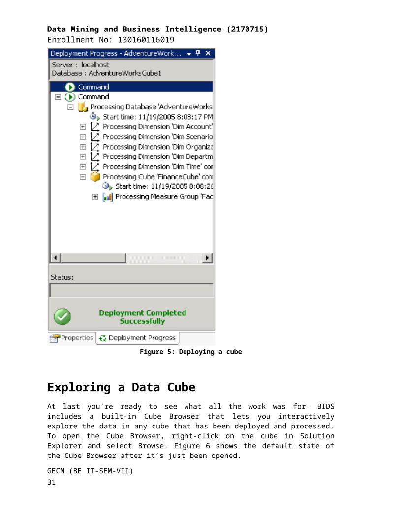
To deploy the cube you just created, select Build ⇒ Deploy AdventureWorksCube1. This will deploy the cube to your local Analysis Server, and also process the cube, building the aggregates for you. BIDS will open the Deployment Progress window, as shown in Figure 5, to keep you informed during deployment and processing.

Figure 5: Deploying a cube



Exploring a Data Cube At last you’re ready to see what all the work was for. BIDS includes a built-in Cube Browser that lets you interactively explore the data in any cube that has been deployed and processed. To open the Cube Browser, right-click on the cube in Solution Explorer and select Browse. Figure 6 shows the default state of the Cube Browser after it’s just been opened. The Cube Browser is a drag-and-drop environment. If you’ve worked with pivot tables in Microsoft Excel, you should have no trouble using the Cube browser. The pane to the left includes all of the measures and dimensions in your cube, and the pane to the right gives you drop targets for these measures and dimensions. Among other operations, you can:

Figure 6: The cube browser in BIDS • Drop a measure in the Totals/Detail area to see the aggregated data for that measure.

• Drop a dimension or level in the Row Fields area to summarize by that level or dimension on rows.



• Drop a dimension or level in the Column Fields area to summarize by that level or dimension on columns

• Drop a dimension or level in the Filter Fields area to enable filtering by members of that dimension or level.

• Use the controls at the top of the report area to select additional filtering expressions.

To see the data in the cube you just created, follow these steps:

1. Right-click on the cube in Solution Explorer and select Browse.

2. Expand the Measures node in the metadata panel (the area at the left of the user interface).

3. Expand the Fact Finance node.

4. Drag the Amount measure and drop it on the Totals/Detail area.

5. Expand the Dim Account node in the metadata panel.

6. Drag the Account Description property and drop it on the Row Fields area.

7. Expand the Dim Time node in the metadata panel.

8. Drag the Calendar Year-Calendar Quarter-Month Number of Year hierarchy and drop it on the Column Fields area.

9. Click the + sign next to year 2001 and then the + sign next to quarter 3.

10. Expand the Dim Scenario node in the metadata panel.

11. Drag the Scenario Name property and drop it on the Filter Fields area.

12. Click the dropdown arrow next to scenario name. Uncheck all of the checkboxes except for the one next to the Budget name.



Figure 7 shows the result. The Cube Browser displays month-by-month budgets by account for the third quarter of 2001. Although you could have written queries to extract this information from the original source data, it’s much easier to let Analysis Services do the heavy lifting for you.

Figure 7: Exploring cube data in the cube browser



EXPERIMENT-5

Aim :- Design and Create cube by identifying measures and dimensions for Design storage for cube using storage mode MOLAP, ROLAP and HOLAP.


Knowledge Required: MOLAP, ROLAP, HOLAP

Theory/Logic:

Partition Storage (SSAS) Physical storage options affect the performance, storage requirements, and storage locations of partitions and their parent measure groups and cubes. A partition can have one of three basic storage modes:

• Multidimensional OLAP (MOLAP)

• Relational OLAP (ROLAP)

• Hybrid OLAP (HOLAP)

Microsoft SQL Server 2005 Analysis Services (SSAS) supports all three basic storage modes. It also supports proactive caching, which enables you to combine the characteristics of ROLAP and MOLAP storage for both immediacy of data and query performance. You can configure the storage mode and proactive caching options in one of three ways.

Storage Configuration Method

Description

Storage Settings dialog

You can configure storage settings for a partition or configure default storage settings for a measure group.

Storage Design Wizard

You can configure storage settings for a partition at the same time that you design aggregations.

You can also define a filter to restrict the source data that is read into the partition using any of the three storage modes.

Usage-Based Optimization Wizard

You can select a storage mode and optimize aggregation design based on queries that have been sent to the cube.



MOLAP

The MOLAP storage mode causes the aggregations of the partition and a copy of its source data to be stored in a multidimensional structure in Analysis Services, which structure is highly optimized to maximize query performance. This can be storage on the computer where the partition is defined or on another Analysis Services computer. Storing data on the computer where the partition is defined creates a local partition. Storing data on another Analysis Services computer creates a remote partition. The multidimensional structure that stores the partition's data is located in a subfolder of the Data folder of the Analysis Services program files or another location specified during setup of Analysis Services.

Because a copy of the source data resides in the Analysis Services data folder, queries can be resolved without accessing the partition's source data even when the results cannot be obtained from the partition's aggregations. The MOLAP storage mode provides the most rapid query response times, even without aggregations, but which can be improved substantially through the use of aggregations.

As the source data changes, objects in MOLAP storage must be processed periodically to incorporate those changes. The time between one processing and the next creates a latency period during which data in OLAP objects may not match the current data. You can incrementally update objects in MOLAP storage without downtime. However, there may be some downtime required to process certain changes to OLAP objects, such as structural changes. You can minimize the downtime required to update MOLAP storage by updating and processing cubes on a staging server and using database synchronization to copy the processed objects to the production server. You can also use proactive caching to minimize latency and maximize availability while retaining much of the performance advantage of MOLAP storage.

ROLAP

The ROLAP storage mode causes the aggregations of the partition to be stored in tables in the relational database specified in the partition's data source. Unlike the MOLAP storage mode, ROLAP does not cause a copy of the source data to be stored in the Analysis Services data folders. When results cannot be derived from the aggregations or query cache, the fact table in the data source is accessed to answer queries. With the ROLAP storage mode, query response is generally slower than that available with the other MOLAP or HOLAP storage modes. Processing time is also typically slower. Realtime ROLAP is typically used when clients need to see changes immediately. No aggregations are stored with real-time ROLAP. ROLAP is also used to save storage space for large datasets that are infrequently queried, such as purely historical data.

Note: When using ROLAP, Analysis Services may return incorrect information related to the unknown member if a join is combined with a group by, which eliminates relational integrity errors rather than returning the unknown member value.

If a partition uses the ROLAP storage mode and its source data is stored in SQL Server 2005 Analysis Services (SSAS), Analysis Services attempts to create indexed views to contain aggregations of the partition. If Analysis Services cannot create indexed views, it does not create aggregation tables. While Analysis Services handles the session requirements for creating indexed views on SQL Server 2005 Analysis Services (SSAS), the creation and use of indexed views for aggregations requires the following conditions to be met by the ROLAP partition and the tables in its schema:



• The partition cannot contain measures that use the Min or Max aggregate functions.

• Each table in the schema of the ROLAP partition must be used only once. For example, the schema cannot contain "dbo"."address" AS "Customer Address" and "dbo"."address" AS "SalesRep Address".

• Each table must be a table, not a view.

• All table names in the partition's schema must be qualified with the owner name, for example, "dbo"."customer".

• All tables in the partition's schema must have the same owner; for example, you cannot have a FromClause like : "tk"."customer", "john"."store", or "dave"."sales_fact_2004".

• The source columns of the partition's measures must not be nullable.

• All tables used in the view must have been created with the following options set to ON:

o ANSI_NULLS o QUOTED_IDENTIFIER • The total size of the index key, in SQL Server 2005, cannot exceed 900 bytes. SQL Server

2005 will assert this condition based on the fixed length key columns when the CREATE INDEX statement is processed. However, if there are variable length columns in the index key, SQL Server 2005 will also assert this condition for every update to the base tables. Because different aggregations have different view definitions, ROLAP processing using indexed views can succeed or fail depending on the aggregation design.

• The session creating the indexed view must have the following options on: ARITHABORT, CONCAT_NULL_YEILDS_NULL, QUOTED_IDENTIFIER, ANSI_NULLS, ANSI_PADDING, and ANSI_WARNING. This setting can be made in SQL Server Management Studio.

• The session creating the indexed view must have the following option off: NUMERIC_ROUNDABORT. This setting can be made in SQL Server Management Studio.

HOLAP

The HOLAP storage mode combines attributes of both MOLAP and ROLAP. Like MOLAP, HOLAP causes the aggregations of the partition to be stored in a multidimensional structure on an Analysis Services server computer. HOLAP does not cause a copy of the source data to be stored. For queries that access only summary data contained in the aggregations of a partition, HOLAP is the equivalent of MOLAP. Queries that access source data, such as a drilldown to an atomic cube cell for which there is no aggregation data, must retrieve data from the relational database and will not be as fast as if the source data were stored in the MOLAP structure.

Partitions stored as HOLAP are smaller than equivalent MOLAP partitions and respond faster than ROLAP partitions for queries involving summary data. HOLAP storage mode is generally suitable for partitions in cubes that require rapid query response for summaries based on a large amount of source data. However, where users generate queries that must touch leaf level data, such as for calculating median values, MOLAP is generally a better choice.



Steps: 1. In the Analysis service object explorer tree pane, expand the Cubes folder, rightclick the

created cube, and then click Property.

2. In the property wizard, select proactive caching and then select option button.



3. Select MOLAP/HOLAP/ROLAP as your data storage type, and then click Next.

4. After setting required parameters, click ok button.

5. After that right click on created cube and then select Process.

Application: -- To analyze data for decision making.



EXPERIMENT-6

Aim :- Process cube and Browse cube data. Perform different operations on cube.

a. By replacing a dimension in the grid, filtering and drilldown using cube browser.

b. Browse dimension data and view dimension members, member properties, member property values.

c. Create calculated member using arithmetic operators and member property of dimension member.


Knowledge Required: Data Mining Concepts Theory/Logic:

Browsing Cube Data Use the Browser tab of Cube Designer to browse cube data. You can use this view to examine the structure of a cube and to check data, calculation, formatting, and security of database objects. You can quickly examine a cube as end users see it in reporting tools or other client applications. When you browse cube data, you can view different dimensions, drill down into members, and slice through dimensions.

Before you browse a cube, you must process it. After you process it, open the Browser tab of Cube Designer. The Browser tab has three panes — the Metadata pane, the Filter pane, and the Data pane. Use the Metadata pane to examine the structure of the cube in tree format. Use the Filter pane at the top of the Browser tab to define any subcube you want to browse. Use the Data pane to examine the data and drill down through dimension hierarchies.

Setting up the Browser

To prepare to browse a cube, you can specify a perspective or translation that you want to use. You add measures and dimensions to the Data pane and specify any filters in the Filter pane.

Specifying a Perspective Use the Perspective list to choose a perspective that is defined for the cube. Perspectives are defined in the Perspectives tab of Cube Designer. To switch to a different perspective, select any perspective in the list.

Specifying a Translation

Use the Language list to choose a translation that is defined for the cube. Translations are defined in the Translations tab of Cube Designer. The Browser tab initially shows captions for the default language, which is specified by the Language property for the cube. To switch to a different language, select any language in the list.

Formatting the Data Pane You can format captions and cells in the Data pane. Right-click the selected cells or captions that you want to format, and then click Commands and Options. Depending on the selection, the



Commands and Options dialog box displays settings for Format, Filter and Group, Report, and Behavior.

Setting up the Data

Adding or Removing Measures

Drag the measures you want to browse from the Metadata pane to the details area of the Data pane, which is labeled Drop Totals or Detail Fields Here. As you drag additional measures, they are added as columns in the details area. A vertical line indicates where each additional measure will drop. Dragging the Measures folder drops all the measures into the details area.

To remove a measure from the details area, either drag it out of the Data pane, or rightclick it and then click Remove Total on the shortcut menu.

Adding or Removing Dimensions

Drag the hierarchies or dimensions to the row or column field areas.

To remove a dimension, either drag it out of the Data pane, or right-click it and then click Remove Field on the shortcut menu.

Adding or Removing Filters

You can use either of two methods to add a filter: • Expand a dimension in the Metadata pane, and then drag a hierarchy to the Filter pane.

- or -

• In the Dimension column of the Filter pane, click <Select dimension> and select a dimension from the list, then click <Select hierarchy> in the Hierarchy column and select a hierarchy from the list.

After you specify the hierarchy, specify the operator and filter expression. The following table describes the operators and filter expressions.

Operator Filter Expression Description

Equal One or members

more Values must be equal to a specified member. (Provides multiple member selection for attribute hierarchies, other than parent-child hierarchies, and single member selection for other hierarchies.)

Not Equal One or members

more Values must not equal a specified member. (Provides multiple member selection for attribute hierarchies, other than parent-child hierarchies, and single member selection for other hierarchies.)

In One or

named sets

more Values must be in a specified named set.

(Supported for attribute hierarchies only.)



Not In One or

named sets

more Values must not be in a specified named set.

(Supported for attribute hierarchies only.)

Range

(Inclusive)

One or

delimiting members range

two

of a

Values must be between or equal to the delimiting members. If the delimiting members are equal or only one member is specified, no range is imposed and all values are permitted.

(Supported only for attribute hierarchies. The

range must be on one level of a hierarchy.

Unbounded ranges are not currently supported.)

Range

(Exclusive)

One or two

delimiting

members of a

range

Values must be between the delimiting members. If the delimiting members are the equal or only one member is specified, values must be either greater than or less than the delimiting member. (Supported only for attribute hierarchies. The range must be on one level of a hierarchy. Unbounded ranges are not currently supported.)

MDX An MDX

expression

returning a

member set

Values must be in the calculated member set. Selecting this option displays the Calculated Member Builder dialog box for creating MDX expressions.

For user-defined hierarchies, in which multiple members may be specified in the filter expression, all the specified members must be at the same level and share the same parent. This restriction does not apply for parent-child hierarchies.

Working with Data

Drilling Down into a Member

To drill down into a particular member, click the plus sign (+) next to the member or double-click the member.



Slicing Through Cube Dimensions

To filter the cube data, click the drop-down list box on the top-level column heading. You can expand the hierarchy and select or clear a member on any level to show or hide it and all its descendants. Clear the check box next to (All) to clear all the members in the hierarchy.

After you have set this filter on dimensions, you can toggle it on or off by right-clicking anywhere in the Data pane and clicking Auto Filter.

Filtering Data You can use the filter area to define a subcube on which to browse. You can add a filter by either clicking a dimension in the Filter pane or by expanding a dimension in the Metadata pane and then dragging a hierarchy to the Filter pane. Then specify an Operator and Filter Expression.

Performing Actions

A triangle marks any heading or cell in the Data pane for which there is an action. This might apply for a dimension, level, member, or cube cell. Move the pointer over the heading object to see a list of available actions. Click the triangle in the cell to display a menu and start the associated process.

For security, the Browser tab only supports the following actions:

• URL

• Rowset

• Drillthrough

Command Line, Statement, and Proprietary actions are not supported. URL actions are only as safe as the Web page to which they link.

Viewing Member Properties and Cube Cell Information

To view information about a dimension object or cell value, move the pointer over the cell.

Showing or Hiding Empty Cells

You can hide empty cells in the data grid by right-clicking anywhere in the Data pane and clicking Show Empty Cells.

c. Create calculated member using arithmetic operators and member property of dimension

member

Calculated members are members of a dimension or a measure group that is defined based on a combination of cube data, arithmetic operators, numbers, and functions. For example, you can create a calculated member that calculates the sum of two physical measures in the cube. Calculated member definitions are stored in cubes, but their values are calculated at query time.

To create a calculated member, use the New Calculated Member command on the Calculations tab of Cube Designer. You can create a calculated member within any dimension, including the measures dimension. You can also place a calculated member within a display folder in the Calculation Properties dialog box.



In the tasks in this topic, you define calculated measures to let users view the gross profit margin percentage and sales ratios for Internet sales, reseller sales, and for all sales.

To define calculations to aggregate physical measures

1. Open Cube Designer for the Analysis Services Tutorial cube, and then click the Calculations tab.

Notice the default CALCULATE command in the Calculation Expressions pane and in the Script Organizer pane. This command specifies that the measures in the cube should be aggregated according to the value that is specified by their AggregateFunction properties. Measure values are generally summed, but may also be counted or aggregated in some other manner.

The following image shows the Calculations tab of Cube Designer.

2. On the toolbar of the Calculations tab, click New Calculated Member. A new form appears in the Calculation Expressions pane within which you define the properties of this new calculated member. The new member also appears in the Script Organizer pane.



The following image shows the form that appears in the Calculation Expressions pane when you click New Calculated Member.

3. In the Name box, change the name of the calculated measure to [Total Sales Amount].

If the name of a calculated member contains a space, the calculated member name must be enclosed in square brackets.

Notice in the Parent hierarchy list that, by default, a new calculated member is created in the Measures dimension. A calculated member in the Measures dimension is also frequently called a calculated measure.

4. On the Metadata tab in the Calculation Tools pane of the Calculations tab, expand Measures and then expand Internet Sales to view the metadata for the Internet Sales measure group.

You can drag metadata elements from the Calculation Tools pane into the Expression box and then add operators and other elements to create Multidimensional Expressions (MDX) expressions. Alternatively, you can type the MDX expression directly into the Expression box.

If you cannot view any metadata in the Calculation Tools pane, click Reconnect on the toolbar. If this does not work, you may have to process the cube or start the instance of


Note:


Analysis Services. 1. Drag Internet Sales-Sales Amount from the Metadata tab in the Calculation Tools pane into

the Expression box in the Calculation Expressions pane.

2. In the Expression box, type a plus sign (+) after [Measures].[Internet SalesSales Amount].

3. On the Metadata tab in the Calculation Tools pane, expand Reseller Sales, and then drag Reseller Sales-Sales Amount into the Expression box in the Calculation Expressions pane after the plus sign (+).

4. In the Format string list, select "Currency".

5. In the Non-empty behavior list, select the check boxes for Internet Sales-Sales

Amount and Reseller Sales-Sales Amount, and then click OK.

The measures you specify in the Non-empty behavior list are used to resolve NON EMPTY queries in MDX. When you specify one or more measures in the Non-empty behavior list, Analysis Services treats the calculated member as empty if all the specified measures are empty. If the Non-empty behavior property is blank, Analysis Services must evaluate the calculated member itself to determine whether the member is empty.

The following image shows the Calculation Expressions pane populated with the settings that you specified in the previous steps.

6. On the toolbar of the Calculations tab, click Script View, and then review the calculation script in the Calculation Expressions pane.

Notice that the new calculation is added to the initial CALCULATE expression; each individual calculation is separated by a semicolon. Notice also that a comment appears at the beginning of the calculation script. Adding comments within the calculation script for groups of calculations is a good practice, to help you and other developers understand complex calculation scripts.



7. Add a new line in the calculation script after the Calculate; command and before the newly added calculation script, and then add the following text to the script on its own line:

/* Calculations to aggregate Internet Sales and Reseller Sales measures */

The following image shows the calculation scripts as they should appear in the Calculation Expressions pane at this point in the tutorial.

8. On the toolbar of the Calculations tab, click Form View, verify that [Total Sales Amount] is selected in the Script Organizer pane, and then click New Calculated Member.

9. Change the name of this new calculated member to [Total Product Cost], and then create the following expression in the Expression box:

[Measures].[Internet Sales-Total Product Cost] + [Measures].[Reseller Sales-Total Product Cost]

10. In the Format string list, select "Currency".

11. In the Non-empty behavior list, select the check boxes for Internet Sales-Total Product Cost and Reseller Sales-Total Product Cost, and then click OK. You have now defined two calculated members, both of which are visible in the Script Organizer pane. These calculated members can be used by other calculations that you define later in the calculation script. You can view the definition of any calculated member by selecting the calculated member in the Script Organizer pane; the definition of the calculated member will appear in the Calculation Expressions pane in the Form view. Newly defined calculated members will not appear in the Calculation Tools pane until these objects have been deployed. Calculations do not require processing.

Defining Gross Profit Margin Calculations To define gross profit margin calculations

1. Verify that [Total Product Cost] is selected in the Script Organizer pane, and then click New Calculated Member on the toolbar of the Calculations tab.

2. In the Name box, change the name of this new calculated measure to [Internet GPM].



3. In the Expression box, create the following MDX expression:

([Measures].[Internet Sales-Sales Amount] - [Measures].[Internet Sales-Total Product Cost]) /

[Measures].[Internet Sales-Sales Amount]

4. In the Format string list, select "Percent".

5. In the Non-empty behavior list, select the check box for Internet Sales-Sales Amount, and then click OK.

6. On the toolbar of the Calculations tab, click New Calculated Member.

7. In the Name box, change the name of this new calculated measure to [Reseller GPM].


([Measures].[Reseller Sales-Sales Amount] - [Measures].[Reseller Sales-Total Product Cost]) /

[Measures].[Reseller Sales-Sales Amount]


10. In the Non-empty behavior list, select the check box for Reseller Sales-Sales Amount, and then click OK.


12. In the Name box, change the name of this calculated measure to [Total GPM].


([Measures].[Total Sales Amount] -

[Measures].[Total Product Cost]) /

[Measures].[Total Sales Amount]

Notice that this calculated member is referencing other calculated members. Because this calculated member will be calculated after the calculated members that it references, this is a valid calculated member.

14. In the Format string list, select "Percent". 15. In the Non-empty behavior list, select the check boxes for Internet Sales-Sales Amount and

Reseller Sales-Sales Amount, and then click OK.

16. On the toolbar of the Calculations tab, click Script View and review the three calculations you just added to the calculation script.

17. Add a new line in the calculation script immediately before the [Internet GPM] calculation, and then add the following text to the script on its own line:

/* Calculations to calculate gross profit margin */



The following image shows the Expressions pane with the three new calculations.

Defining the Percent of Total Calculations

To define the percent of total calculations

1. On the toolbar of the Calculations tab, click Form View.

2. In the Script Organizer pane, select [Total GPM], and then click New Calculated Member on the toolbar of the Calculations tab.

Clicking the final calculated member in the Script Organizer pane before you click New Calculated Member guarantees that the new calculated member will be entered at the end of the script. Scripts execute in the order that they appear in the Script Organizer pane.

3. Change the name of this new calculated member to [Internet Sales Ratio to All Products]. 4. Type the following expression in the Expression box:

Case

When IsEmpty( [Measures].[Internet Sales-Sales Amount] )

Then 0

Else ( [Product].[Product Categories].CurrentMember,

[Measures].[Internet Sales-Sales Amount]) /

( [Product].[Product Categories].[(All)].[All],

[Measures].[Internet Sales-Sales Amount] )

End



This MDX expression calculates the contribution to total Internet sales of each product. The Case statement together with the IS EMPTY function ensures that a divide by zero error does not occur when a product has no sales.


6. In the Non-empty behavior list, select the check box for Internet Sales-Sales Amount, and then click OK.


8. Change the name of this calculated member to [Reseller Sales Ratio to All Products].

9. Type the following expression in the Expression box:

Case

When IsEmpty( [Measures].[Reseller Sales-Sales Amount] )

Then 0


[Measures].[Reseller Sales-Sales Amount]) /


[Measures].[Reseller Sales-Sales Amount] ) End


11. In the Non-empty behavior list, select the check box for Reseller Sales-Sales Amount, and then click OK.

12. On the toolbar of the Calculations tab, click New Calculated Member. 13. Change the name of this calculated member to [Total Sales Ratio to All Products].

14. Type the following expression in the Expression box:

Case

When IsEmpty( [Measures].[Total Sales Amount] )

Then 0


[Measures].[Total Sales Amount]) /


[Measures].[Total Sales Amount] ) End


16. In the Non-empty behavior list, select the check boxes for Internet Sales-Sales Amount and Reseller Sales-Sales Amount, and then click OK.



17. On the toolbar of the Calculations tab, click Script View, and then review the three calculations that you just added to the calculation script.

18. Add a new line in the calculation script immediately before the [Internet Sales Ratio to All Products] calculation, and then add the following text to the script on its own line:

/* Calculations to calculate percentage of product to total product sales */

You have now defined a total of eight calculated members, which are visible in the Script Organizer pane when you are in Form view.

Browsing the New Calculated Members To browse the new calculated members

1. On the Build menu of Business Intelligence Development Studio, click Deploy Analysis Services Tutorial.

2. When deployment has successfully completed, switch to the Browser tab, click Reconnect, and then remove all hierarchies and measures from the Data pane.

3. In the Metadata pane, expand Measures to view the new calculated members in the Measures dimension.

4. Add the Total Sales Amount, Internet Sales-Sales Amount, and Reseller SalesSales Amount measures to the data area, and then review the results.

Notice that the Total Sales Amount measure is the sum of the Internet SalesSales Amount measure and the Reseller Sales-Sales Amount measure.

5. Add the Product Categories user-defined hierarchy to the filter area of the Data pane, and then filter the data by Mountain Bikes.

Notice that the Total Sales Amount measure is calculated for the Mountain Bikes category of product sales based on the Internet Sales-Sales Amount and the Reseller Sales-Sales Amount measures for Mountain Bikes.

6. Add the Date.Calendar Time user-defined hierarchy to the row area, and then review the results.

Notice that the Total Sales Amount measure for each calendar year is calculated for the Mountain Bikes category of product sales based on the Internet SalesSales Amount and the Reseller Sales-Sales Amount measures for Mountain Bikes.

7. Add the Total GPM, Internet GPM, and Reseller GPM measures to the data area, and then review the results.

Notice that the gross profit margin for reseller sales is significantly lower than for sales over the Internet. Notice also that the gross profit margin on the sales of mountain bikes is increasing over time, as shown in the following image.



8. Add the Total Sales Ratio to All Products, Internet Sales Ratio to All Products, and Reseller Sales Ratio to All Products measures to the data area. Notice that the ratio of the sales of mountain bikes to all products has increased over time for Internet sales, but is decreasing over time for reseller sales. Notice also that the ratio of the sale of mountain bikes to all products is lower from sales through resellers than it is for sales over the Internet.

9. Change the filter from Mountain Bikes to Bikes, and review the results. Notice that the gross profit margin for all bikes sold through resellers is negative, because touring bikes and road bikes are being sold at a loss. 10. Change the filter to Accessories, and then review the results.

Notice that the sale of accessories is increasing over time, but that these sales make up only a small fraction of total sales. Notice also that the gross profit margin for sales of accessories is higher than for bikes.

10. Expand CY 2004, expand H2 CY 2004, and then expand Q3 CY 2004.

Notice that there are no Internet sales in this cube for after July, 2004, and no reseller sales for after June, 2004. These sales values have not yet been added from the source systems to the Adventure Works DW database.

EXPERIMENT-7



Aim :- Design and create data mining models using Analysis Service of SQL Server 2005


Knowledge Required: Data Mining Models Theory/Logic:

The tutorial is broken up into three sections.

1. Preparing the SQL Server Database,

2. Preparing the Analysis Services Database, and

3. Building and Working with the Mining Models.

Preparing the SQL Server Database

The AdventureWorksDW database, which is the basis for this tutorial, is installed with SQL Server (not by default, but as an option at installation time) and already contains views that will be used to create the mining models. If it was not installed at the installation time, you can add it by selecting Change button from Control Panel Æ Add/Remove Programs Æ Microsoft SQL Server 2005.

Preparing the Analysis Services Database

Before you begin to create and work with mining models, you must perform the following tasks:

1. Create a new Analysis Services project

2. Create a data source.

3. Create a data source view.

a) Creating an Analysis Services Project

Each Analysis Services project defines the schema for the objects in a single Analysis Services database. The Analysis Services database is defined by the mining models, OLAP cubes, and supplemental objects that it contains.

To create an Analysis Services project

4. Open Business Intelligence Development Studio.

5. Select New and Project from the File menu. 6. Select Analysis Services Project as the type for the new project and name it AdventureWorks.

7. Click Ok.

The new project opens in Business Intelligence Development Studio.

b) Creating a Data Source



A data source is a data connection that is saved and managed within your project and deployed to your Analysis Services database. It contains the server name and database where your source data resides, as well as any other required connection properties. To create a data source

1. Right-click the Data Source project item in Solution Explorer and select New Data Source.

2. On the Welcome page, click Next.

3. Click New to add a connection to the AdventureWorksDW database.

4. The Connection Manager dialog box opens. In the Server name drop-down box, select the server where AdventureWorksDW is hosted (for example, localhost), enter your credentials, and then in the Select the database on the server drop-down box select the AdventureWorksDW database.

5. Click OK to close the Connection Manager dialog box.

6. Click Next.

7. By default the data source is named Adventure Works DW. Click Finish The new data source, Adventure Works DW, appears in the Data Sources folder in Solution Explorer.

c) Creating a Data Source View

A data source view provides an abstraction of the data source, enabling you to modify the structure of the data to make it more relevant to your project. Using data source views, you can select only the tables that relate to your particular project, establish relationships between tables, and add calculated columns and named views without modifying the original data source.

To create a data source view 1. In Solution Explorer, right-click Data Source View, and then click New Data Source View. 2. On the Welcome page, click Next.

3. The Adventure Works DW data source you created in the last step is selected by default in the Relational data sources window. Click Next.

4. If you want to create a new data source, click New Data Source to launch the Data Source Wizard.

5. Select the tables in the following list and click the right arrow button to include them in the new data source view:

6. vAssocSeqLineItems

7. vAssocSeqOrders

8. vTargetMail

9. vTimeSeries

10. Click Next.

11. By default the data source view is named Adventure Works DW. Click Finish. Data Source View Editor opens to display the Adventure Works DW data source view, as shown in Figure 2. Solution Explorer is also updated to include the new data source view.



Figure 2: Adventure Works DW data source view

Building and Working with the Mining Models The data mining editor (shown in Figure 3) contains all of the tools and viewers that you will use to build and work with the mining models.



Figure 3: Data mining editor

EXPERIMENT-8



Aim :- To study data mining MDX query language.

Software Required: Analysis Services - SQL Server 2005 Knowledge Required: Query language Theory/Logic:

Data Mining Extensions (DMX) is a language that you can use to create and work with data mining models in Microsoft SQL Server 2005 Analysis Services (SSAS). You can use DMX to create the structure of new data mining models, to train these models, and to browse, manage, and predict against them. DMX is composed of data definition language (DDL) statements, data manipulation language (DML) statements, and functions and operators.

Microsoft OLE DB for Data Mining Specification

The data mining features in Analysis Services are built to comply with the Microsoft OLE DB for Data Mining specification, which was first released to coincide with the release of Microsoft SQL Server 2000.

The Microsoft OLE DB for Data Mining specification defines the following:

• A structure to hold the information that defines a data mining model.

• A language for creating and working with data mining models.

The specification defines the basis of data mining as the data mining model virtual object. The data mining model object encapsulates all that is known about a particular mining model. The data mining model object is structured like an SQL table, with columns, data types, and meta information that describe the model. This structure lets you use the DMX language, which is an extension of SQL, to create and work with models.

DMX Statements

You can use DMX statements to create, process, delete, copy, browse, and predict against data mining models. There are two types of statements in DMX: data definition statements and data manipulation statements. You can use each type of statement to perform different kinds of tasks.

The following sections provide more information about working with DMX statements:

• Data Definition Statements • Data Manipulation Statements • Query Fundamentals

Data Definition Statements



Use data definition statements in DMX to create and define new mining structures and models, to import and export mining models and mining structures, and to drop existing models from a database. Data definition statements in DMX are part of the data definition language (DDL).

You can perform the following tasks with the data definition statements in DMX:

• Create a mining structure by using the CREATE MINING STRUCTURE (DMX) statement, and add a mining model to the mining structure by using the ALTER MINING STRUCTURE (DMX) statement.

• Create a mining model and associated mining structure simultaneously by using the CREATE MINING MODEL (DMX) statement to build an empty data mining model object.

• Export a mining model and associated mining structure to a file by using the EXPORT (DMX) statement. Import a mining model and associated mining structure from a file that is created by the EXPORT statement by using the IMPORT (DMX) statement.

• Copy the structure of an existing mining model into a new model, and train it with the same data, by using the SELECT INTO (DMX) statement.

• Completely remove a mining model from a database by using the DROP MINING MODEL (DMX) statement. Completely remove a mining structure and all its associated mining models from the database by using the DROP MINING STRUCTURE (DMX) statement.

Data Manipulation Statements

Use data manipulation statements in DMX to work with existing mining models, to browse the models and to create predictions against them. Data manipulation statements in DMX are part of the data manipulation language (DML).

You can perform the following tasks with the data manipulation statements in DMX:

• Train a mining model by using the INSERT INTO (DMX) statement. This does not insert the actual source data into a data mining model object, but instead creates an abstraction that describes the mining model that the algorithm creates. The source query for an INSERT INTO statement is described in <source data query>.

• Extend the SELECT statement to browse the information that is calculated during model training and stored in the data mining model, such as statistics of the source data. Following are the clauses that you can include to extend the power of the SELECT statement: o SELECT DISTINCT FROM <model > (DMX) o SELECT FROM <model>.CONTENT (DMX) o SELECT FROM <model>.CASES (DMX) o SELECT FROM <model>.SAMPLE_CASES (DMX) o SELECT FROM <model>.DIMENSION_CONTENT (DMX)

• Create predictions that are based on an existing mining model by using the PREDICTION JOIN clause of the SELECT statement. The source query for a PREDICTION JOIN statement is described in <source data query>.

• Remove all the trained data from a model or a structure by using the DELETE (DMX) statement.



DMX Query Fundamentals

The SELECT statement is the basis for most DMX queries. Depending on the clauses that you use with such statements, you can browse, copy, or predict against mining models. The prediction query uses a form of SELECT to create predictions based on existing mining models. Functions extend your ability to browse and query the mining models beyond the intrinsic capabilities of the data mining model.

You can use DMX functions to obtain information that is discovered during the training of your models, and to calculate new information. You can use these functions for many purposes, including to return statistics that describe the underlying data or the accuracy of a prediction, or to return an expanded explanation of a prediction.

Working with data mining models in Microsoft SQL Server 2005 Analysis Services (SSAS) involves the following primary tasks:

• Creating mining structures and mining models

• Processing mining structures and mining models

• Deleting or dropping mining structures or mining models

• Copying mining models

• Browsing mining models

• Predicting against mining models

You can use Data Mining Extensions (DMX) statements to perform each of these tasks programmatically. Creating mining structures and mining models Use the CREATE MINING STRUCTURE (DMX) statement to add a new mining structure to a database. You can then use the ALTER MINING STRUCTURE (DMX) statement to add mining models to the mining structure.

Use the CREATE MINING MODEL (DMX) statement to build a new mining model and associated mining structure.

Processing mining structures and mining models Use the INSERT INTO (DMX) statement to process a mining structure and mining model.

Deleting or dropping mining structures or mining models Use the DELETE (DMX) statement to remove all the trained data from a mining model or mining structure. Use the DROP MINING STRUCTURE (DMX) or DROP MINING MODEL (DMX) statements to completely remove a mining structure or mining model from a database.

Copying mining models



Use the SELECT INTO (DMX) statement to copy the structure of an existing mining model into a new mining model and to train the new model with the same data.

Browsing mining models Use the SELECT (DMX) statement to browse the information that the data mining algorithm calculates and stores in the data mining model during model training. Much like with Transact-SQL, you can use several clauses with the SELECT statement, to extend its power. These clauses include DISTINCT FROM <model>, FROM <model>.CASES, FROM <model>.SAMPLE_CASES, FROM <model>.CONTENT and FROM <model>.DIMENSION_CONTENT.

Predicting against mining models Use the PREDICTION JOIN clause of the SELECT statement to create predictions that are based on an existing mining model.

You can also import and export models by using the IMPORT (DMX) and EXPORT (DMX) statements.

These tasks fall into two categories, data definition statements and data manipulation statements, which are described in the following table.

Statements model or creating predictions.


Topic Description Data Mining Extensions (DMX) Data DefinitionStatements

Part of the data definition la nguage (DDL). Used to define a new mining model (including training) or to drop an existing mining model from a database.

Data Mining Extensions(DMX) Data Manipulation

Part of the data manipulation language (DML). Used work with existing mining models, including browsing a


Creating DMX Prediction Queries

The main goal of most data mining projects is to use mining models to create predictions for new data. For example, you may want to predict how many bicycles your company will sell next year during December, or whether a potential customer will purchase a bicycle in response to an advertising campaign. You can also use predictions to explore the information that the algorithms discover when they train the mining models.

Prediction queries are based on the Data Mining Extensions (DMX) language. DMX extends the SQL language, to provide support for working with mining models.

Prediction Query Tools

SQL Server provides two tools that you can use to build prediction queries: Prediction Query Builder and the Query Editor. Prediction Query Builder is included in the Mining Model Prediction tab of Data Mining Designer. When you use the query builder, you can use graphical tools to design a query, use a text editor to manually modify the query, and use a simple results pane to view the results of the query. The Query Editor provides tools that you can use to build and run DMX queries.

You can also include prediction queries as part of a SQL Server 2005 Integration Services (SSIS) package.

The main goal of most data mining projects is to use mining models to create predictions for new data. For example, you may want to predict how many bicycles your company will sell next year during December, or whether a potential customer will purchase a bicycle in response to an advertising campaign. You can also use predictions to explore the information that the algorithms discover when they train the mining models.

Prediction queries are based on the Data Mining Extensions (DMX) language. DMX extends the SQL language, to provide support for working with mining models.

Prediction Query Tools

SQL Server provides two tools that you can use to build prediction queries: Prediction Query Builder and the Query Editor. Prediction Query Builder is included in the Mining Model Prediction tab of Data Mining Designer. When you use the query builder, you can use graphical tools to design a query, use a text editor to manually modify the query, and use a simple results pane to view the results of the query. The Query Editor provides tools that you can use to build and run DMX queries.

You can also include prediction queries as part of a SQL Server 2005 Integration Services (SSIS) package.

Data Mining Extensions (DMX) Function Reference Analysis Services supports several functions in the Data Mining Extensions (DMX) language. Functions expand the results of a prediction query to include information that further describes the prediction. Functions also provide more control over how the results of the prediction are returned.



The following table lists the functions that DMX supports.

Function Description BottomCount Returns a table that contains a specified number of

bottommost rows, in increasing order of rank based on a rank expression.

BottomPercent Returns a table that contains the smallest number of bottommost rows that meet a specified percent expression, increasing order of rank based on a rank expression.

BottomSum Returns a table that contains the smallest number of bottommost rows that meet a specified sum expression, in increasing order of rank based on a rank expression.

Cluster Returns the cluster that is most likely to contain the input case.

ClusterProbability Returns the probability that the input case belongs to the cluster.

IsDescendant Indicates whether the current node descends from the specified node.

IsInNode Indicates whether the specified node contains the case.

Lag Returns the time slice between the date of the current case and the last date in the data.

Predict Performs a prediction on a specified column.

PredictAdjustedProbability Returns the adjusted probability of the specified predictable column.

PredictAssociation Predicts associative membership in a column.

PredictCaseLikelihood Returns the likelihood that an input case will f it within the existing model. This function can only be used with clustering models.

PredictHistogram Returns a table that represents the histogram for a specified column.

PredictNodeId Returns the NodeID for a selected case.

PredictProbability Returns the probability of the specified column.



EXPERIMENT-9

Aim :- To implement any one data mining algorithms in any programming language.

Apriori Algorithm

#include<stdio.h>int l2[10][2],memberinl2;bool isPresent(int a,int b){

for(int i=1;i<=memberinl2;i++){

if(l2[i][0]==a){

if(l2[i][1]==b){

return true;}

}}return false;

}


PredictSequence Predicts the next values in a sequence.

PredictStdev Retrieves the standard deviation value for a specified column.

PredictSupport Returns the support value of the column.

PredictTimeSeries Predicts the future values for a time series.

PredictVariance Returns the variance value of the specified column.

RangeMax Returns the upper value of the predicted bucket that discovered for a specified discretized column.

RangeMid Returns the midpoint value of the predicted bucket that discovered for a specified discretized column.

RangeMin Returns the lower value of the predicted bucket that discovered for a specified discretized column.

TopCount Returns a table that contains a specified number of topmost rows, in a decreasing order of rank based on a rank expression.

TopPercent Returns a table that contains the smallest number of topmost rows that meet a specified percent expression, in a decreasing order of rank based on a rank expression.

TopSum Returns a table that contains the smallest number of topmost rows that meet a specified sum expression, in a decreasing order of rank based on a rank expression.


bool isProper(int a,int b,int c){

if(isPresent(a,b)){

if(isPresent(b,c)){

if(isPresent(a,c)){

return true;}

}}return false;

}

int main(){int i,j,temp=0,count=0,min_sup=2;int t[10][4]={{-1,-1,-1,-1},{1,2,5,0},{2,4,0,0},{2,3,0,0},{1,2,4,0},{1,3,0,0},{2,3,0,0},{1,3,0,0}, {1,2,3,5},{1,2,3,0}};

printf("Apriori algorithm\n");printf("--------------------------------\n");printf("\nTransactions\n\n");

for(i=1;i<10;i++){printf("t%d :- \t",i);

for(j=0;j<4;j++){

if(t[i][j]==0)continue;

printf("%d\t",t[i][j]);}

printf("\n");}

printf("--------------------------------\n");printf("\n\nCandidate 1 itemset:-\n\n");

int totalitems=5;

int countofc1[totalitems+1],c1[totalitems+1];

for(i=1;i<totalitems+1;i++){

countofc1[i]=0;c1[i]=i;



}

for(i=1;i<10;i++){

for(j=0;j<4;j++){

temp=t[i][j];countofc1[temp]++;

}}

for(i=1;i<totalitems+1;i++){

printf("{%d}-->%d\n",i,countofc1[i]);if(countofc1[i]>=min_sup)

count++;}

int l1[count+1],countofl1[count+1];int p=1;

for(i=1;i<6;i++){

if(countofc1[i]>=min_sup){l1[p]=c1[i];countofl1[p]=countofc1[i];p++;}

}

printf("--------------------------------\n");printf("\n\nFrequent 1 itemset:-\n\n");

for(i=1;i<=count;i++){

printf("{%d}-->%d\n",l1[i],countofl1[i]);}

int totalinl1=count;

int memberinc2=0;

while(totalinl1!=0){memberinc2=memberinc2+(totalinl1-1);totalinl1--;}

totalinl1=5;



//printf("%d",memberinc2);

int c2[memberinc2+1][2],countofc2[memberinc2+1];j=1;

for(int i=1;i<totalinl1;i++){

for(int k=i+1;k<=totalinl1;k++){

c2[j][0]=l1[i];c2[j][1]=l1[k];j++;

}}

for(i=1;i<=10;i++){

countofc2[i]=0;}

for(i=1;i<=10;i++){

for(int k=1;k<10;k++){

for(j=0;j<4;j++){

if(t[k][j]==c2[i][0]){

for(j=0;j<4;j++){if(t[k][j]==c2[i][1]){countofc2[i]++;}}

}}

}}

printf("--------------------------------\n");printf("\n\nCandidate 2-itemset:-\n\n");

count=0;for(i=1;i<=10;i++){

printf("{%d,%d}-->%d\n",c2[i][0],c2[i][1],countofc2[i]);if(countofc2[i]>=2)

count++;}

//int l2[count+1][2],memberinl2=count;int countofl2[count+1];



int c=1;for(i=1;i<=10;i++){

if(countofc2[i]>=2){

l2[c][0]=c2[i][0];l2[c][1]=c2[i][1];countofl2[c]=countofc2[i];c++;

}}printf("--------------------------------\n");printf("\n\nFrequent 2 itemset:-\n\n");

for(i=1;i<c;i++){

printf("{%d,%d}-->%d\n",l2[i][0],l2[i][1],countofl2[i]);}

int totalinl2=memberinl2;

count=0;int c3[totalinl2][3];

for(int i=1;i<totalinl2;i++){

for(int k=i+1;k<=totalinl2;k++){

if(l2[i][0]==l2[k][0] && l2[i][1]<l2[k][1]){

if(isProper(l2[i][0],l2[i][1],l2[k][1])){

count++;c3[count][0]=l2[i][0];c3[count][1]=l2[i][1];c3[count][2]=l2[k][1];

}

}}

}

printf("--------------------------------\n");printf("\n\nCandidate 3-itemset:-\n\n");

int countofc3[3];

for(i=1;i<=2;i++){

countofc3[i]=0;}



for(i=1;i<=2;i++){

for(int k=1;k<10;k++){

for(j=0;j<4;j++){

if(t[k][j]==c3[i][0]){

for(j=0;j<4;j++){

if(t[k][j]==c3[i][1]){

for(j=0;j<4;j++){

if(t[k][j]==c3[i][2]){

countofc3[i]++;}

}}

}}

}}

}

count=0;for(i=1;i<3;i++){

printf("{%d,%d,%d}-->%d\n",c3[i][0],c3[i][1],c3[i][2],countofc3[i]);if(countofc3[i]>=2)

count++;}

int l3[count+1][3],countofl3[count+1];c=1;for(i=1;i<=count;i++){

if(countofc3[i]>=2){

l3[c][0]=c3[i][0];l3[c][1]=c3[i][1];l3[c][2]=c3[i][2];countofl3[c]=countofc3[i];c++;

}

}printf("--------------------------------\n");



printf("\n\nFrequent 3 itemset:-\n\n");

for(int j=1;j<c;j++){

printf("{%d,%d,%d}-->%d\n",l3[j][0],l3[j][1],l3[j][2],countofl3[j]);}

return 0;}OUTPUT:

EXPERIMENT-10

Aim :- To perform hand on experiments with sample data sets on XLMiner.

XLMiner is the only comprehensive data mining add-in for Excel, with neural nets, classification and regression trees, logistic regression, linear regression, Bayes classifier, K-nearest neighbors, discriminant analysis, association rules, clustering, principal components, and more.

XLMiner provides everything you need to sample data from many sources -- PowerPivot, Microsoft/IBM/Oracle databases, or spreadsheets; explore and visualize your data with multiple linked charts; preprocess and 'clean' your data, fit data mining models, and evaluate your models' predictive power.

Sample Data Sets:

T1= {M, O, N, K, E, Y}T2= {D, O, N, K, E, Y}T3= {M, U, C, K, Y}T4= {M, A, K, E}T5= {C, O, K, I, E}

Steps:



1. Open XLMiner then from the file menu open new file.2. Define the item sets as shown in figure 1.

Figure 1

3. From Add-Ins tab choose XLMInerAffintyAssociation Rules as shown in figure 2.



Figure 2

4. From Parameters define minimum support and minimum confidence for mining as shown in figure 3.

Figure 3

5. Association Rules will be shown like figure 4.



Figure 4

EXPERIMENT-11

AIM : Create an .arff file for following attributes and study histogram for that data.

Weather outlook, temperature, humidity, windy and play

Solution:

@relation weather

@attribute outlook {sunny, overcast, rainy}@attribute temperature {hot, mild, cool}@attribute humidity {high, normal}@attribute windy {TRUE, FALSE}@attribute play {yes, no}

@datasunny,hot,high,FALSE,nosunny,hot,high,TRUE,noovercast,hot,high,FALSE,yesrainy,mild,high,FALSE,yes



rainy,cool,normal,FALSE,yesrainy,cool,normal,TRUE,noovercast,cool,normal,TRUE,yessunny,mild,high,FALSE,nosunny,cool,normal,FALSE,yesrainy,mild,normal,FALSE,yessunny,mild,normal,TRUE,yesovercast,mild,high,TRUE,yesovercast,hot,normal,FALSE,yesrainy,mild,high,TRUE,no

Histogram for Outlook:



Histogram for Temperature:

Histogram for humidity:



Histogram for windy:

Histogram for play:



Visualization of all:

EXPERIMENT-12(a)

Aim :- To perform Association Rule Mining experiment with sample data sets in weka.

Step 1: Choose dataset.



Step 2: Choose Apriori algorithm.



Step 3: Set measures.

Step 4 : List of Generated Rules



EXPERIMENT-12(b)



AIM : Implement classification with Decision tree in weka.

Step 1 : Open Weka Explorer Preprocess Go to Open files and select proper file.

Step 2 : Go to Classify Choose Tree Choose Id3.



Step 3 : Select Use training set Start.

Step 4 : Select Cross-validation Start.



Step 5 : Select Percentage split Start.



Step 6 : Go to Classify Choose Tree Choose J48 Select Use training set Start.

Step 7 : Select Cross-validation Start.



Step 8 : Select Percentage split Start.

Visualize tree



EXPERIMENT-12(c)

AIM : Demonstration of classification rule process on dataset weather.nominal.arff using naïve bayes algorithm.

Step 1: Select database



Step 2: Choose Algorithm and Classify.



EXPERIMENT-13

Aim :- To study two research papers related to data mining and derive conclusions in your own language.



EXPERIMENT-14

Aim :- Make a presentation on any one Advance topic.

TOPIC:


helpgecmit.files.wordpress.com · web viewaim : create an .arff file for following attributes and...

Documents