viewing (perspective) the graphics · pdf file–history of computer graphics ......

© 2012 Kavita Bala •(with previous instructors James/Marschner)

Cornell CS4620/5620 Fall 2012 • Lecture 11 1

CS4620/5620: Lecture 11

Viewing (Perspective)The Graphics Pipeline


Cornell CS4620/5620 Fall 2012 • Lecture 11

Announcements

• Friday– History of Computer Graphics

• Wednesday– HW 1 is due– PPA 1 is out

2



Pipeline of transformations

• Standard sequence of transforms

3

!

!

!

!

!

!

!

!

7.1. Viewing Transformations 147

object space

world space

camera space

canonicalview volume

scre

en

sp

ace

modelingtransformation

viewporttransformation

projectiontransformation

cameratransformation

Figure 7.2. The sequence of spaces and transformations that gets objects from their

original coordinates into screen space.

space) to camera coordinates or places them in camera space. The projection

transformation moves points from camera space to the canonical view volume.

Finally, the viewport transformation maps the canonical view volume to screen Other names: camera

space is also “eye space”

and the camera

transformation is

sometimes the “viewing

transformation;” the

canonical view volume is

also “clip space” or

“normalized device

coordinates;” screen space

is also “pixel coordinates.”

space.

Each of these transformations is individually quite simple. We’ll discuss them

in detail for the orthographic case beginning with the viewport transformation,

then cover the changes required to support perspective projection.

7.1.1 The Viewport Transformation

We begin with a problemwhose solution will be reused for any viewing condition.

We assume that the geometry we want to view is in the canonical view volume The word “canonical” crops

up again—it means

something arbitrarily

chosen for convenience.

For instance, the unit circle

could be called the

“canonical circle.”

and we wish to view it with an orthographic camera looking in the !z direction.The canonical view volume is the cube containing all 3D points whose Cartesian

coordinates are between !1 and +1—that is, (x, y, z) " [!1, 1]3 (Figure 7.3).We project x = !1 to the left side of the screen, x = +1 to the right side of thescreen, y = !1 to the bottom of the screen, and y = +1 to the top of the screen.

Recall the conventions for pixel coordinates fromChapter 3: each pixel “owns”

a unit square centered at integer coordinates; the image boundaries have a half-

unit overshoot from the pixel centers; and the smallest pixel center coordinates



Orthographic transformation chain

• Start with coordinates in object’s local coordinates• Transform into world coords (modeling transform, Mm)

• Transform into eye coords (camera xf., Mcam = Fc–1)

• Orthographic projection, Morth

• Viewport transform, Mvp

4

⇤

⌥⌥⇧

xs

ys

zc

1

⌅

��⌃ =

⇤

⌥⌥⇧

nx2 0 0 nx�1

2

0 ny

2 0 ny�12

0 0 1 00 0 0 1

⌅

��⌃

⇤

⌥⌥⇧

2r�l 0 0 � r+l

r�l

0 2t�b 0 � t+b

t�b

0 0 2n�f �n+f

n�f

0 0 0 1

⌅

��⌃

�u v w e0 0 0 1

⇥�1

Mm

⇤

⌥⌥⇧

xo

yo

zo

1

⌅

��⌃

ps = MvpMorthMcamMmpo



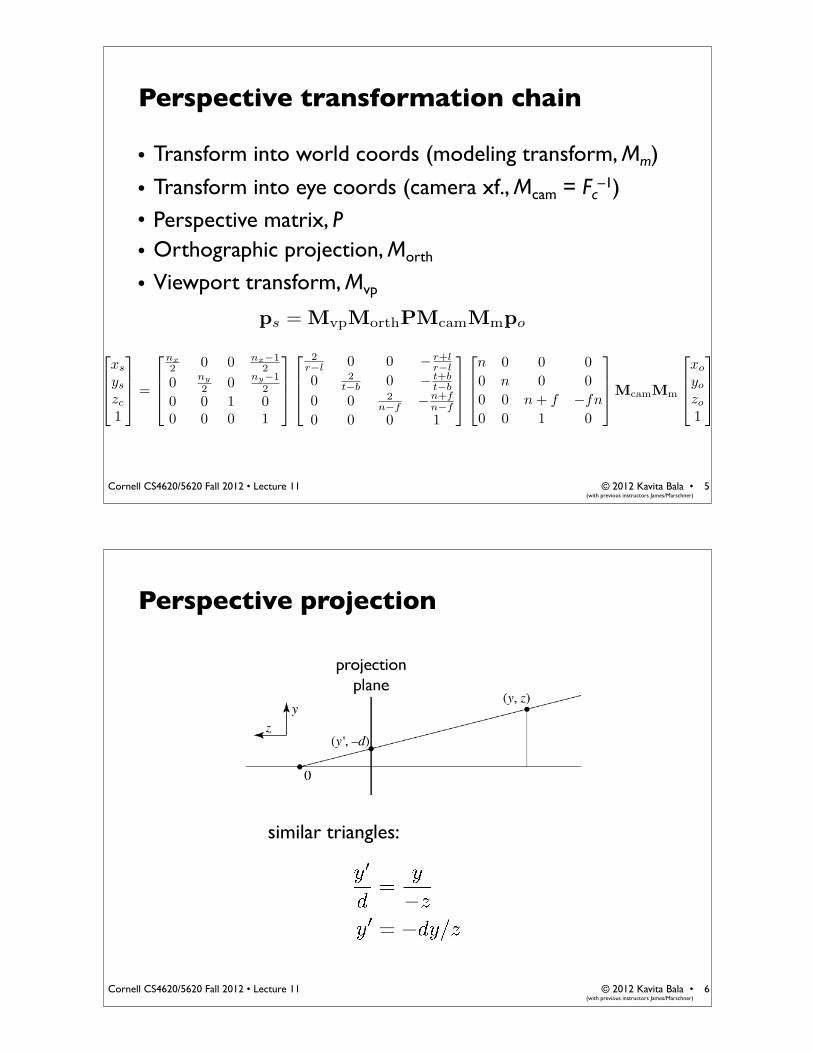
Perspective transformation chain

• Transform into world coords (modeling transform, Mm)


• Perspective matrix, P• Orthographic projection, Morth


5

ps = MvpMorthPMcamMmpo

�

⇧⇧⇤

xs

ys

zc

1

⇥

⌃⌃⌅ =

�

⇧⇧⇤

nx2 0 0 nx�1

2

0 ny

2 0 ny�12

0 0 1 00 0 0 1

⇥

⌃⌃⌅

�

⇧⇧⇤

2r�l 0 0 � r+l

r�l

0 2t�b 0 � t+b

t�b

0 0 2n�f �n+f

n�f

0 0 0 1

⇥

⌃⌃⌅

�

⇧⇧⇤

n 0 0 00 n 0 00 0 n + f �fn0 0 1 0

⇥

⌃⌃⌅McamMm

�

⇧⇧⇤

xo

yo

zo

1

⇥

⌃⌃⌅



Perspective projection

similar triangles:

6



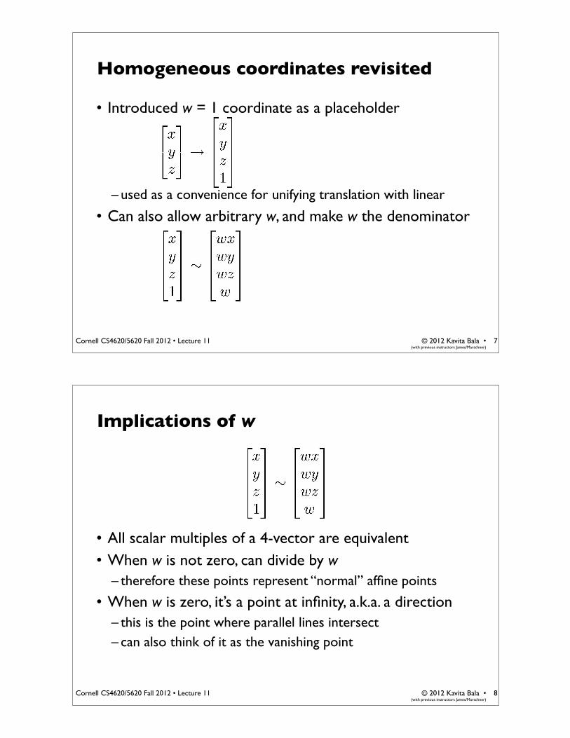
Homogeneous coordinates revisited

• Introduced w = 1 coordinate as a placeholder

– used as a convenience for unifying translation with linear

• Can also allow arbitrary w, and make w the denominator

7



Implications of w

• All scalar multiples of a 4-vector are equivalent• When w is not zero, can divide by w

– therefore these points represent “normal” affine points

• When w is zero, it’s a point at infinity, a.k.a. a direction– this is the point where parallel lines intersect– can also think of it as the vanishing point

8



Mas

acci

o, T

rini

ty, F

lore

nce



Projective Plane

• When W is not 0, the point represented is (X/W, Y/W) in the Euclidean plane

• When W is 0, the point represented is a point at infinity (direction)

• Note that the triple (0, 0, 0) is omitted and does not represent any point

• The origin is represented by (0, 0, 1)

10



Perspective projection

to implement perspective, just move z to w:

11



View volume: perspective

12



View volume: perspective (clipped)

13



Carrying depth through perspective

• Perspective has a varying denominator—can’t preserve depth!• Compromise: preserve depth on near and far planes

– that is, choose a and b so that z’(n) = n and z’(f) = f.

14



Official perspective matrix

• Use near plane distance as the projection distance– i.e., d = –n

• Scale by –1 to have fewer minus signs– scaling the matrix does not change the projective

transformation

15

P =

�

⇧⇧⇤

n 0 0 00 n 0 00 0 n + f �fn0 0 1 0

⇥

⌃⌃⌅



Perspective projection matrix

• Product of perspective matrix with orth. projection matrix

16

Mper = MorthP

=

�

⇧⇧⇧⇤

2r�l 0 0 � r+l

r�l

0 2t�b 0 � t+b

t�b

0 0 2n�f �n+f

n�f

0 0 0 1

⇥

⌃⌃⌃⌅

�

⇧⇧⇤

n 0 0 00 n 0 00 0 n + f �fn0 0 1 0

⇥

⌃⌃⌅

=

�

⇧⇧⇧⇧⇤

2nr�l 0 l+r

l�r 0

0 2nt�b

b+tb�t 0

0 0 f+nn�f

2fnf�n

0 0 1 0

⇥

⌃⌃⌃⌃⌅



Perspective transformation chain

• Transform into world coords (modeling transform, Mm)


• Perspective matrix, P• Orthographic projection, Morth


17

ps = MvpMorthPMcamMmpo

�

⇧⇧⇤

xs

ys

zc

1

⇥

⌃⌃⌅ =

�

⇧⇧⇤

nx2 0 0 nx�1

2

0 ny

2 0 ny�12

0 0 1 00 0 0 1

⇥

⌃⌃⌅

�

⇧⇧⇤

2r�l 0 0 � r+l

r�l

0 2t�b 0 � t+b

t�b

0 0 2n�f �n+f

n�f

0 0 0 1

⇥

⌃⌃⌅

�

⇧⇧⇤

n 0 0 00 n 0 00 0 n + f �fn0 0 1 0

⇥

⌃⌃⌅McamMm

�

⇧⇧⇤

xo

yo

zo

1

⇥

⌃⌃⌅



OpenGL view frustum: orthographic

Note OpenGL puts the near and far planes at –n and –fso that the user can give positive numbers

18



OpenGL view frustum: perspective

Note OpenGL puts the near and far planes at –n and –fso that the user can give positive numbers

19



Pipeline of transformations

• Standard sequence of transforms

20

!

!

!

!

!

!

!

!

7.1. Viewing Transformations 147

object space

world space

camera space

canonicalview volume

scre

en

sp

ace

modelingtransformation

viewporttransformation

projectiontransformation

cameratransformation

Figure 7.2. The sequence of spaces and transformations that gets objects from their

original coordinates into screen space.

space) to camera coordinates or places them in camera space. The projection

transformation moves points from camera space to the canonical view volume.

Finally, the viewport transformation maps the canonical view volume to screen Other names: camera

space is also “eye space”

and the camera

transformation is

sometimes the “viewing

transformation;” the

canonical view volume is

also “clip space” or

“normalized device

coordinates;” screen space

is also “pixel coordinates.”

space.

Each of these transformations is individually quite simple. We’ll discuss them

in detail for the orthographic case beginning with the viewport transformation,

then cover the changes required to support perspective projection.

7.1.1 The Viewport Transformation

We begin with a problemwhose solution will be reused for any viewing condition.

We assume that the geometry we want to view is in the canonical view volume The word “canonical” crops

up again—it means

something arbitrarily

chosen for convenience.

For instance, the unit circle

could be called the

“canonical circle.”

and we wish to view it with an orthographic camera looking in the !z direction.The canonical view volume is the cube containing all 3D points whose Cartesian

coordinates are between !1 and +1—that is, (x, y, z) " [!1, 1]3 (Figure 7.3).We project x = !1 to the left side of the screen, x = +1 to the right side of thescreen, y = !1 to the bottom of the screen, and y = +1 to the top of the screen.

Recall the conventions for pixel coordinates fromChapter 3: each pixel “owns”

a unit square centered at integer coordinates; the image boundaries have a half-

unit overshoot from the pixel centers; and the smallest pixel center coordinates



CS4620/5620

Pipeline



The graphics pipeline

• The standard approach to object-order graphics• Many versions exist

– software, e.g. Pixar’s REYES architecture• many options for quality and flexibility

– hardware, e.g. graphics cards in PCs• amazing performance: millions of triangles per frame

• We’ll focus on an abstract version of hardware pipeline

22



The graphics pipeline

• “Pipeline” because of the many stages– very parallelizable– leads to remarkable performance of graphics cards (many times

the flops of the CPU at ~1/3 the clock speed)– gigaflops (10 to the 9th power), teraflop (12th power), petaflops

(15th power)

• GeForce GTX690, 915MHz, 2x1536 stream processors

23



Supercomputers

• Tesla K10– Peak performance

• 4577 Gigaflops• 3072 cores (1536/GPU)

• Tianhe-1A, Tesla: 14,336 Xeon + 7,1688 Tesla boards – 448 cores (2 petaflops)

• Current supercomputer– IBM Sequoia (petascale) Blue Gene (16 petaflops)

24



Primitives• Points• Line segments

– and chains of connected line segments

• Triangles• And that’s all!

– Curves? Approximate them with chains of line segments– Polygons? Break them up into triangles– Curved regions? Approximate them with triangles

• Hardware desire: minimal primitives– simple, uniform, repetitive: good for parallelism– and of course, cyclical; now you can send curves, and the vertex

shader will convert to primitives25



Rasterization

• First job: enumerate the pixels covered by a primitive– simple, aliased definition: pixels whose centers fall inside

• Second job: interpolate values across the primitive– e.g. colors computed at vertices– e.g. normals at vertices– will see applications later on

26



Rasterizing lines

• Define line as a rectangle

• Specify by two endpoints

• Ideal image: black inside, white outside

27



Point sampling

• Approximate rectangle by drawing all pixels whose centers fall within the line

• Problem: sometimes turns on adjacent pixels

28



Point samplingin action

29

viewing (perspective) the graphics · pdf file–history of computer graphics ......

Documents