vii. an empirical analysis of the dutch fdi activities ... · 95 vii. an empirical analysis of the...

95

VII.An empirical analysis of the Dutch FDI activities 1984-2002

7.1 Introduction

In Chapter 6 I briefly reviewed the most important theoretical aspects of Foreign Di-rect Investments and the Knowledge-Capital (K-K) Model in detail and also I attempted to identify the most important factors and variables affecting investment decisions. In this chapter I apply empirical methods to answer the following research questions:

• What is the relationship between the Dutch FDI and trade? This question frequently arises in the literature, and there is evidence for both substitution and complementar-ity. The direction of this causal relationship can be related to the investment motives.

• What are the main determinants of the out- and inward FDI activities from/to the

Netherlands, in other words, what are the main motives behind investments? The causal relationship between FDI and trade may give us hints about the main motives behind FDI activities, but whether this is related to a tariff-jumping, an efficiency- orresource-seeking strategy can be decided on ground of a structural model only.

• Finally, do the European economic (EEC/EU) and monetary (EMU) integration have any significant impact on the Dutch FDI activities? On ground of the K-K model, onehas reason to expect that both EEC and EMU lead to a rise of the vertical multination-als while the weight of horizontal MNEs decreases. If this really happened so, the EEC or the EMU should not only have a positive impact on the value of FDI, but also affect its relationship with foreign trade.

The chapter is structured as follows: Section 7.2 briefly reviews the data sources andprovides a general picture about the evolution of Dutch FDI activities in the last twenty years. In Section 7.3, after a short literature overview, I carry out a causality test in order to obtain a clear picture about the relationship between foreign trade and FDI. In Section 7.4, I will estimate static and dynamic panel model for both out- and inward FDI and look for answers to the above-mentioned research questions. Finally, Section 7.5 summarizes the findings.

7.2 Data and sources

In this chapter, similarly to many empirical works, I use FDI stock data rather than flows. The main reason is that flows may often be negative (caused by repatriation of

Péter Földvári The Economic Impact of the European Integration on the Netherlands

96

profits for example), while stocks are strictly positive.1 This enables one to loglinearize the empirical model, which makes the estimation more convenient.

The panel for outward FDI consists of 37 countries and 19 years (1984-2002), while the panel for inward FDI has 23 countries and 19 years. The reason for the difference in the number of countries is that inward FDI are more concentrated geographically than outward FDI. In 2000, for example, the five most important sources and destinations ofFDI (the USA, Belgium, Germany, the United Kingdom, and France) accounted for about 63.6 percent of the total Dutch FDI stocks abroad and roughly 71.6 percent of the foreign FDI stocks in the Netherlands (see Table 7.1). The evolution of the share of different continents and country-groups in total FDI stocks, however, shows a quite similar picture (see Figure 7.1a and b).

Table 7.1Share of different sources and destinations of Dutch FDI in 2000

Partner Share in Dutch FDI stocks abroad

Share in foreign FDI stocks in the Netherlands

USA 25.8% 21.5%Belgium 10.9% 15.7%

United Kingdom 10.6% 15.6%Germany 10.2% 13.7%France 6.1% 5.1%

Top5 total 63.6% 71.6%Other EU 13% 11.8%EU total 50.8% 61.9%

Europe other 9.6% 6%Asia 6% 4.5%

Rest of the World 7.8% 6.2%

Source: De Nederlandsche BankNote that the table is constructed so that it does not add up to 100%.

1 I omit those observations however where the FDI stock is zero. This is a general practice in empirical research even though leads to a sample-selection bias.

Chapter 7 A theoretical approach to Foreign Direct Investments

97

Figure 7.1aThe geographical distribution of Dutch FDI stock abroad (outward FDI stocks)1984-2002

Source: De Nederlandsche Bank

Figure 7.1bThe geographical distribution of foreign FDI stock in the Netherlands (inward FDI stocks)1984-2002

Source: De Nederlandsche Bank

In both figures one can observe a significant increase of the share of EU members,apparently mostly at the expense of the United States: the US investors’ share in total FDI


98

stocks in the Netherlands falls from 36% in 1984 to 21.2% in 2002. The weight of USA as a destination of Dutch FDI also decreases significantly from 49.2% in 1984 to 20.3%in 2002. In the same period the share of EU countries in total incoming FDI stock grows steadily from 34.8% to 63.9%, and the share of EU countries in total Dutch outward FDI stocks expands from 31% to 52.3%. Whether this is an impact of the European integration is a main question of this chapter. An important difference is that while the share of non-EU member European countries increased in total Dutch FDI stocks abroad, their share decreased in the foreign FDI stocks in the Netherlands. It appears as if the increase of the share of EU members occurred also at the expense of non-EU members. One should not forget, however, that both in 1986 and 1995 new members joined the EU and this resulted upward shift in the share of the European Union. The sum of the shares of EU members and other European countries increases in both figures, which indicates that the share ofEurope increased at the expense of other continents.

Data on the Dutch FDI (both stocks and flows) is available online on the homep-age of De Nederlandsche Bank (http://www.dnb.nl). The collection of FDI statistics is, however, often problematic, and one may find serious differences between the theoreticaland statistical definition of foreign direct investments. The widely accepted definitionof Foreign Direct Investments states that “FDI occurs when an investor based in one country, acquires an asset in another country with the intent to manage that asset.”2 As the FDI statistics are collected as part of the balance of payment statistics according to IMF guidelines, an increase in the FDI does not necessarily mean that a new investment really took place. A large share of FDI flows occur in order to acquire existing firms orfinance merger operations, without directly creating a new stock of assets. Another sourceof measurement problems is that profits of foreign-owned firms are generally measured asoutflows from the host country, while undivided profits are taken into account as inwardFDI, even though there is no guarantee that these resources will be spent on investments. Also, if a foreign-owned affiliate borrows from the host-country, it will also appear in theFDI statistics as inward investment. Problems may arise from different institutional and legal structures too. For example, some may regard 20% foreign ownership as the lower limit of a firm being under foreign control, others may find the threshold being at 50%(see South Centre, 1997).

These differences in national rules and definitions should not cause any problem fornow, since only the definitions of the De Nederlandsche Bank are used. According to this,all transactions that are meant to acquire or found an enterprise with the intent to manage it, and also all financial transactions between the owner company and its affiliates countas FDI.

The GDP and GDP per capita are taken from the Groningen Growth and Development Center (http://www.ggdc.nl). The real exchange rates are calculated from the data avail-able in the Penn World Table 6.1 (http://pwt.econ.upenn.edu). The data on the average years of schooling are from the Barro-Lee dataset3

2 World Trade Organization: Annual Report, Vol.1. Trade and Foreign Direct Investment, WTO, Geneva3 There are other similar datasets available, for example that of Domenech and de la Fuente (2002), still the data of Barro and Lee are still the most widely used.


99

(http://www.cid.harvard.edu/ciddata//Appendix%20Data%20Tables.xls), which provides data for each fifth year only. I use the “spline smoothing” function of the GiveWin2 tointerpolate the missing observations. The data on the competitive position of the Neth-erlands expressed as annual change in percentages are published as Appendix B1 in the Central Economisch Plan (Central Economic Plan) by the Centraal Planbureau (http://www.cpb.nl/nl/data/cep2005/b1.xls). The competitive position of the Netherlands indica-tor is calculated as the difference of the average annual change of unit labor costs in the competitor countries and in the Netherlands. Consequently, a negative value indicates that the unit labor costs increases in the Netherlands at a higher pace than in the rest of the World, which has a detrimental impact on the competitiveness of Dutch goods. This indicator is applied as a proxy for the relative efficiency of the Dutch producers. The datasources and conversion methods are summarized in the Appendix.

7.3 Does FDI cause trade or vica versa? A causality analysis.

7.3.1 Substitutes or complements?

Before building an empirical model for FDI, an important question arises, namely the direction of causal relationship between FDI and foreign trade. As it was shown in the previous chapter, the expectations about the direction of causal relationship between trade and FDI depend mainly on the incentives behind FDI.

In case of horizontal (or tariff-jumping) FDI, multinationals move their production abroad because the variable costs of exporting (tariffs and transaction costs) are high enough to make it profitable. From this perspective one can expect that exports and FDIare negatively related, that is, FDI is a substitute for exports. In other words, as the Heck-sher-Ohlin Model suggests, factor movements eliminate the price differentials and there-fore the reason for trade (Mundell, 1957).

On the other hand, theories concerning the possession of intangible assets (Dunning, 1981; Caves, 1982), or increasing returns to scale (Helpman, 1984; Helpman and Krug-man, 1985) all support the possibility that outward FDI and exports are complements. Ethier (1986) shows that under uncertainty, FDI between countries with similar endow-ments becomes higher in both directions, paired with an increasing intra-industry and intra-firm trade. The K-K Model (Markusen, 1997) that was reviewed in detail in theprevious chapter, also suggests that under liberal investment policy and gradually liberal-ized international trade one may expect the increase of vertical FDI activities and foreign trade (exports) at the expense of horizontal MNEs. This should also lead to the further strengthening of the complementary relationship.

Many empirical studies appear to confirm the complementarity hypothesis. Lipseyand Weiss (1981, 1984) carry out a cross-section analysis for the year 1970 and found exclusively positive coefficients (not all are significant though). Blomström et al. (1988)use data for the FDI from the USA and Sweden in the period 1978-1982, and find apositive relationship between exports and FDI, which is especially evident, when FDI is regressed on the change of exports. Furthemore, Yamawaki (1991), Pfaffermayr (1994, 1996) and Bajo-Rubio and Montero-Munoz (2001) also find evidence that FDI and ex-


100

ports are complements, however, only Pfaffermayr (1994, 1996) and Bajo-Rubio and Montero-Munoz apply Granger causality tests for Austria and Spain respectively.

There are results, which question complementarity though: Kim and Rang (1997) use a cross-section approach for South-Korea and Japan cannot find any relationship betweenexports and outward FDI. The work of Beers et al. (1996) is especially important for this dissertation as they estimate an empirical model on the Dutch exports and imports to/from 11 partners in the period 1986-1996 with the out- and inward FDI among the regressors. They find the impact of outward FDI stock on exports significant and negative, whichalso indicates a relationship of substitution. In case of imports, however, the relationship between inward FDI and imports is found to be positive and significant, an evidence infavor of complementarity.

Independently of the interpretation of results, however, the link between FDI and for-eign trade seems to be firmly confirmed. Aizenman and Noy (2005) apply disaggregatedtrade and FDI data to analyze the two-way relationship between trade and investments. Using a decomposition method proposed by Geweke (1982) they find that 81% of thefeedback observed between trade and FDI are attributable to a two-way Granger causality while the rest is explained by the simultaneous correlation of the time-series.

In the followings, I carry out a Granger causality test for the outward FDI and exports of the Netherlands in the period 1984-2002. On ground of the previous chapter and the results from earlier studies, the following hypotheses can be formed about the causal re-lationship between outward FDI (inward FDI) and exports (imports):

• Hypothesis 1: It is expected that outward (inward) FDI causes exports (imports), that is there is a positive, statistically significant causal relationship. This would reinforcethe complementariness hypothesis. Pfaffermayr (1994) could not reject the existence of such a causal link for Austria at 10% level of significance, and Bajo-Rubio andMontero-Munoz (2001) found the same for Spain.

• Hypothesis 2: It is less straightforward whether exports (imports) also cause outward (inward) FDI. If exports are indeed market signals, the relationship should be positive. Bajo-Rubio and Muntero-Munoz, however, cannot confirm the existence of such acausal relationship in Spain, and Pfaffermayr found it to be negative for Austria.

• Hypothesis 3: As a third possible outcome, one may hypothesize that a two-way rela-tionship exists between outward (inward) FDI and exports (imports). In case of time-series analysis or with a panel with a longer time dimension one can even go further and expect cointegration (a long-run equilibrial relationship between FDI and trade). The evidence for cointegration would indicate that there is a long-run equilibrium between FDI and foreign trade. The results are contradictory though: Pfaffermayr cannot confirm that outward FDI and exports are cointegrated, while Bajo-Rubio andMontero-Munoz actually find a cointegrating relationship for Spain.


101

7.3.2. A test of causal relationship

My approach is somewhat different from that of Pfaffermayr (1994, 1996) and Bajo-Rubio and Montero-Munoz (2001): they applied time-series analysis while I opt for a panel causality test. This decision is motivated by the relatively short observation period (19 years). The panel applied for this analysis has consequently a relatively small time dimension but contains 37 countries. As such, it is not likely that foreign trade and FDI are found cointegrated.

The Granger test was used in Chapter 3 already to explore the relationship between openness and per capita GDP growth, and there I presented the main idea behind this causality test. In short, if one finds that the past values of process X can significantlyexplain the variation of the present value of Y, one can argue that X Granger causes Y. Pfaffermayr (1994) proposes the use of a third variable for Granger causality tests in or-der to avoid the omitted variable bias. In case of an open economy, one may assume that GDP affects both FDI and exports, and omitting it would result in a biased estimation. For this reason, I will carry out the Granger test both with and without the GDP as third regressor (Y).

The causality regressions are the following (if GDP is included):

(7.1)

and

(7.2)

Where Yi,t denote the Dutch FDI stock in country i (outward FDI), or the foreign FDI stock in the Netherlands (inward FDI) originated from country i in year t. Xi,t denotes the exports to or the imports from country i respectively, while Zi,t denotes GDP of the country i in year t. The variable ηi denotes the country-specific effect that is a fixed-effectsspecification is used. The strict exogeneity of the regressors is assumed.

A simple GLS estimation of the transformed equations would be biased, since the lagged endogenous variable is correlated with the lagged error-term (Nickell, 1981). This bias diminishes as the time dimension of the panel gets large, but as the T is just 19, it is necessary to apply the GMM-SYS estimation proposed by Arellano and Bover (1995), Blundell and Bond (1998), or a bias-correction method suggested by Kiviet (1995) and Bun and Kiviet (2003). The standard Arellano-Bond (1991) estimator assumes the fol-lowing standard moment restrictions:


102

(7.3)

The GMM-SYS estimator utilizes not only transformed but also level equations and therefore is more efficient than the Arellano-Bond estimator. The additional restrictionsare:

(7.4)

As (7.3) suggests, almost all lagged values of the endogenous variable can be used as instrument. Using all available lags however results in too many instruments, which is the reason why I choose to maximize the number of lags used for instrumentation at 2. Furthermore, I assume the strict exogeneity of the log of GDP (that is I use it as a standard instrument):

(7.5)The estimation yields the following results (I report the coefficients of the parsimoni-

ous regressions, that is, the model is reduced until only significant coefficients remain),from a two-step GMM-SYS estimation:

Table 7.2aResults of the Granger causality test without GDP as exogenous regressor

exports→FDIout FDIout→exports imports→FDIin FDIin→imports

α10.701***

(6.50)0.628***

(4.66)0.958***

(42.98)1.018***

(33.80)

α2 - 0.253*

(2.00) - -

α30.208***

(4.34)0.164**

(2.36)- -

γ10.117*

(1.72) - 0.061*

(1.77) -

γ2 - -0.034*

(-1.88) - -0.023*

(-2.00)

AR(1) -1.30(p=0.194)

-1.90*

(p=0.057)-3.21***

(p=0.001)-3.25***

(p=0.001)

AR(2) -0.81(p=416)

0.05(p=0.964)

0.02(p=0.520)

0.79(p=0.429)

Hansen-test of overi-dent. restrictions

36.73 (d.f.=89)

36.03 (d.f.=88)

22.30(d.f.=96)

22.94(d.f.=96)

Exclusion F-test of the γ coefficients

2.95*

(d.f.= 1, 36)3.53*

(d.f.= 1, 36)3.15*

(d.f.= 1, 22)3.98*

(d.f.=1, 22)

Note: Robust t-statistics are reported in parentheses. All coefficients and statistics reported are from the two-stepestimation, where robust standard errors are finite sample corrected by the method of Windmeijer (2000).***,**,* denote that the coefficient is significant at 1, 5, 10 percent level of significance respectively.


103

Table 7.2bResults of the Granger causality test with GDP as exogenous regressor

Exports→FDIout FDIout→exports imports→FDIin FDIin→imports

α10.695***

(5.77)0.606***

(4.71)0.948***

(30.19)0.999***

(25.07)

α2 - 0.255**

(2.04) - -

α30.184***

(3.33)0.125*

(1.95) - -

β 0.042(0.93)

0.029(1.60)

-0.028(-0.80)

0.013(0.57)

γ10.066(0.96)

0.027**

(2.12) - -

γ2 - -0.060**

(-2.28)0.111(1.43)

-0.019**

(-1.58)

AR(1) -1.29(p=0.197)

-1.92*

(p=0.054)-3.24***

(p=0.001)-3.24***

(p=0.001)

AR(2) -0.82(p=0.410)

-0.07(p=0.943)

0.03(p=0.505)

0.78 (p=0.434

Hansen-test of overident. restrictions

35.96(d.f.= 89)

36.75(d.f.= 87)

22.09(d.f.=96)

22.84(d.f.=96)

Exclusion F-test of the γ coefficients

0.91(d.f.= 3, 36)

4.33**

(d.f.= 2, 36)2.04

(d.f.= 1, 22)2.50

(d.f.=1, 22)

Note: Robust t-statistics are reported in parentheses. All coefficients and statistics reported are from the two-stepestimation, where robust standard errors are finite sample corrected by the method of Windmeijer (2000).***,**,* denote that the coefficient is significant at 1, 5, 10 percent level of significance respectively.

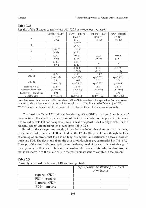
The results in Table 7.2b indicate that the log of the GDP is not significant in any ofthe equations. It seems that the inclusion of the GDP is much more important in time-se-ries causality tests but has no apparent role in case of a panel based Granger-test. For this reason, I accept and interpret the results from Table 7.2a.

Based on the Granger-test results, it can be concluded that there exists a two-way causal relationship between FDI and trade in the 1984-2002 period, even though the lack of cointegration means that there is no long-run equilibrial relationship between foreign trade and FDI. The decisions about the causal relationships are summarized in Table 7.3. The sign of the causal relationship is determined on ground of the sum of the jointly signif-icant gamma coefficients. If their sum is positive, the causal relationship is also positive,that is an increase of the X variable in the past increases the Y variable in the present.

Table 7.3Causality relationships between FDI and foreign trade

Sign of causal relationship at 10% of significance

exports→FDIout +FDIout→exports -Imports→FDIin +FDIin→imports -


104

Exports appear to have a positive effect on outward FDI, which coincides with what Pfaffermayr (1994) and Bajo-Rubio and Montero-Munoz (2001) found for Austria and Spain.4 Export therefore indeed seems to function as market-signal, and consequently has a positive impact on outward FDI.

The results show, however, that outward FDI negatively Granger-causes exports. This finding is similar to Pfaffermayr (1994) who also finds a negative causal relationship fromFDI toward exports in Austria, reinforcing the substitution hypothesis. On the other hand, Bajo-Rubio and Montero-Munoz provides evidence in favor of both short- and long-run positive causal relationship (complementarity). It can be concluded that this result indi-cate substitution in case of outward FDI and exports.

As for imports the direction of causal relationships is basically the same. Imports in-deed Granger-cause inward FDI, but with a positive sign: imports tend to increase future inward investments. The results suggest inward FDI having a negative impact on the imports, which is indicative of substitution again.

The final conclusion is that the Granger tests seem to confirm all hypotheses exceptcointegration. Both out- and inward FDI Granger cause exports and imports, indicating a substitution relationship. This is somewhat different from what Beers et al. find. Theirresults confirm substitution in case of outward FDI and exports, but complementarity incase of inward FDI and imports. Most likely this difference is caused by the different estimation techniques and the difference in the sample size.

The significant substitution relationship is indicative that the majority of investmentswere horizontal. This appears to be a quite general among developed countries both in- and outside the EU, even though, this contradicts the theoretical expectations: in Chapter 6 the K-K Model indicated that trade liberalization should lead to a dominance of vertical FDI and a gradual disappearance of vertical FDI. This does not seem to have happened, but before drawing final conclusions I turn to a more detailed panel analysis.

7.4 A panel analysis of FDI

7.4.1. Model specifications

In this section, an empirical model is applied to explore the motives behind foreign direct investments. As shown in Chapter 6, one may need to include the lagged value of FDI in the right-hand side of our regression, which makes the model dynamic. This is important because of the agglomeration effect and also because investments are expected to be at least partly lumpy and inflexible.

Also as market-related variables such as GDP and population are thought to be an important determinant of Foreign Direct Investments, the empirical model is gravity-like. I estimate the following dynamic models with and without the interaction variable:

4 Bajo-Rubio and Montero-Munoz found that exports affect FDI positively only in the long-run, and they found no relationship in the short-run. Since in this case no cointegration is found, one can conclude that only a short-run relationship exists.


105

(7.6)

and

(7.7)

The notation is summarized in Table 7.4:

Table 7.4Notation and variables in the FDI models

Variable Description Variable Description

FDIi,tout

Dutch FDI stocks in country i in year t concpos,t

The competitive position of the Netherlands in year t. (see Section

7.2)

FDIi,tout FDI stocks in the Netherlands

originated from country i in year t schoolyearsi,t

The ratio of the average educational attainment expressed in years in country i and the Netherlands in

year t.

Yi,tYNL

t

GDP of country i in year t, superscript “NL” denotes the

NetherlandsEECi,t

Dummy variable, set to unity if country i is a member of the EEC/

EU in year t. POPi,tPOPNL

t

population of country i in year t, superscript “NL” denotes the

NetherlandsEMUi,t

Dummy variable, set to unity if country i is a member of the EMU

in year t.

EXPi,t

Exports from the Netherlands to country i in year t (in millions of

1990 USD)EXPi,t·EECi,t

Interaction variable for the relationship between EEC

membership and the impact of exports on outward FDI.

IMPi,t

Imports from country i in year t to the Netherlands (in millions of

1990 USD)IMPi,t·EECi,t

Interaction variable for the relationship between EEC

membership and the impact of imports on inward FDI.

REXCHi,t

Real exchange rate between the guilder and country i’s currency

in year t. trendt Time trend

The use of the first lags exports and imports are important because of the possibleendogenous relationship between FDI and trade. Because of the only time-variant Dutch specific variables I include no year dummies in the regression but attempt to capture theunobserved time-varying effect with the help of a linear time trend (a higher order poly-nomial time trend proved to be insignificant). With help of models (7.6) and (7.7), I testthe following five hypotheses:


106

• Hypothesis 1 assumes that both outward and inward FDI can be modeled by a very simple gravity-like equation with market-related variables (GDP, population) among the regressors. This assumption is very general in FDI modeling, and is supported by a considerable amount of empirical evidence (see Chapter 6). Furthermore, market-size is suggested to be of importance in the Knowledge-Capital (K-K) Model of Markusen (1997, 2002), as discussed in Chapter 6. Both GDP and population capture a different aspect of market size. The Dutch GDP and population (YNL

t and POPNLt) are also im-

portant variables because the K-K Model emphasizes the relative differences in size.

• Hypothesis 2 assumes that the real exchange rate (REEXCHi,t) is an important factor that influences the decision of investors. The direction of the impact of real exchangerate on FDI depends strongly on the relationship between FDI and trade: in case of substitution, for example, the sign of the coefficient should be exactly the opposite ofwhat one would obtain in an export (import) regression. The same sign, on the other hand, reinforces the complementarity relationship. This variable is also connected to the K-K Model since real exchange rates are generally regarded as important compo-nents of transaction costs.

• Hypothesis 3 is related to the main motives behind foreign investments. For this pur-pose two variables are used in the regression: the competitive position of the Neth-erlands (concpost), and the logarithm of the ratio of the average schooling years in a partner country and the Netherlands (schoolyearsi,t). This latter is again directly related to the Knowledge-Capital Model discussed in Chapter 6. Markusen’s model implies that the relative abundance in skills might be of importance for FDI. In other words, these variables are used to test for the “efficiency-seeking”, and the “resource-seeking” hypothesis. At least one of these coefficients is expected to be positive andsignificant.

• Hypothesis 4 assumes that the EEC and EMU membership results in a positive shift in the value of FDI. Therefore, I include the EECi,t and the EMUi,t dummies. It is ex-pected that both variables have a significant positive impact on both out- and inwardFDI. These policy variables represent institutional factors that directly affect transac-tion costs and the freedom of capital flows. Therefore they can also be considered aspractical counterparts of a key factor of the K-K Model: the degree of liberalization of trade and capital flows.

• Finally, Hypothesis 5 assumes that complementary relationship between exports (im-ports) and outward (inward) FDI strengthens over time. Namely, this is what one can expect on ground of the Scenarios 3 and 4 of the K-K model: the simulations indicate that when the free flow of capital is paired by trade liberalization, horizontal FDIsgradually cease to exist. As horizontal FDI is substitute for foreign trade, the positive relationship between exports (imports) and outward (inward) FDI should be stron-ger within the EU. In order to test this hypothesis, a cross-effect variable EEC·EXP (EEC·IMP) is included in the empirical model.


107

7.4.2 Estimation

The above mentioned dynamic specification is essentially Partial Adjustment Models(PAM), as I demonstrate below. Before doing so, one has to make two assumptions: there is an equilibrium level of FDI stock (FDI*), and the FDI stock tends to move toward this equilibrium but this process requires time. Algebraically:

(7.8)where

(7.9)

The coefficient φ reflects the speed of adjustment. Convergence requires that0<|φ|<1.

(7.8) and (7.9) after some transformations yields:(7.10)

Where ηi denotes the individual (country-specific) effect. Also it is assumed that theequilibrium value of FDI stock depends on some exogenous regressors (X) and the indi-vidual effects αi:

(7.11)or using another notation.

(7.12)The speed of adjustment can be calculated as 1/(1-γ) and is expressed in years. This

can be interpreted as the time needed for the system to return to its equilibrium, or as the time which is needed for the impact of an innovation to completely wear out. β denote the short-term impacts of the exogenous variables on lnFDI, and β/(1-γ) are the long-term im-pacts of an exogenous regressor on lnFDI and the equilibrium FDI stock ceteris paribus in an AR(1) specification. Equation (7.11) states implicitly that the speed of adjustment isthe same for all countries. Finally, the strict exogeneity of the regressors is assumed.

Unlike in Chapter 5, the time dimension of the panel is relatively low, 19 years, and therefore one may not hope that the bias in the dynamic panel estimation is negligible.5 Consequently, the coefficients from the GMM-SYS estimation are reported only. Againthe length of the dependent variable used as instruments is maximized at 2. Furthermore, I treat the two population variables as strictly exogenous, and the two GDP variables as predetermined, that is their first lag is used as instrument.

5 Using the formula of Nickell (1981) for the magnitude of bias, I calculated that the bias would be about -0.0937, under the assumption of an autoregressive coefficient 0.5. In other words, the relative bias is almost20%.


108

7.4.3. Results

The results from the estimation of the outward FDI model are reported in the Table 7.5 below. In the third column I report the parsimonious version of the dynamic model, that is, all regressors of the original model with a t-statistics less than one is excluded.

Table 7.5Estimation results from the outward FDI model. GMM-SYS estimation. The dependent variable is Ln(FDIi,t

out)Dynamic

GMM-SYSDynamic with

interaction variableParsimonious

dynamic model

ln(FDIi,t-1out) 0.516**

(2.51)0.520**

(2.68)0.671***

(7.66)

ln(Yi,t)0.603**

(2.65)0.640**

(2.44)0.597***

(3.04)

Ln(YNLt)

0.140(0.10)

0.233(0.16)

2.514***

(3.17)

ln(POPi,t)-0.378**

(-2.05)-0.394*

(-2.01)-0.403***

(-3.09)

Ln(POPNLt)

-0.637(-0.41)

-0.751(-0.49)

-2.951***

(-3.37)

lnEXPi,t-10.188(0.75)

0.157(0.57) -

lnREXCHi,t-0.041(-0.88)

-0.033(-0.69) -

concpost0.009***

(3.20)0.009*

(1.91)0.006**

(2.73)

ln(schoolyearsi,t)0.583(0.67)

0.648(0.74)

-

EECi,t-0.045(-0.10)

0.119(0.17) -

EMUi,t-0.217(0.86)

-0.135(0.17)

-0.289(-1.03)

trendt0.063**

(2.10)0.056(1.52)

ln(EECi,t-1·lnEXPi,t-1) - -0.005(-0.04) -

AR(1) -1.27[p=0.205]

-1.28[p=0.201]

-1.32[p=0.188]

AR(2) -0.99[p=0.325]

-0.98[p=0.329]

-1.05[p=0.295]

Hansen-test of overidentification

27.36(d.f.=33)

25.34(d.f.=32)

33.46(d.f.=4)

Note: Robust t-statistics are reported in parentheses. All coefficients and statistics reported are from the two-stepestimation, where robust standard errors are finite sample corrected by the method of Windmeijer (2000). ***,**,* denote coefficients significant at 1, 5 and 10% respectively.

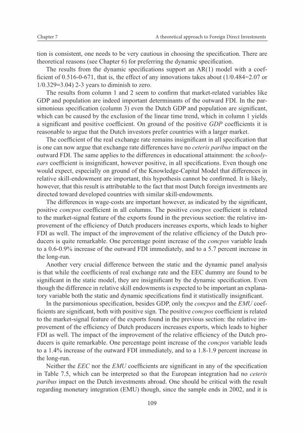
One can observe in Table 7.5 that the lagged dependent variable yields significantcoefficients. Even if one can argue that the Within-Group estimator in a static specifica-


109

tion is consistent, one needs to be very cautious in choosing the specification. There aretheoretical reasons (see Chapter 6) for preferring the dynamic specification.

The results from the dynamic specifications support an AR(1) model with a coef-ficient of 0.516-0-671, that is, the effect of any innovations takes about (1/0.484=2.07 or1/0.329=3.04) 2-3 years to diminish to zero.

The results from column 1 and 2 seem to confirm that market-related variables likeGDP and population are indeed important determinants of the outward FDI. In the par-simonious specification (column 3) even the Dutch GDP and population are significant,which can be caused by the exclusion of the linear time trend, which in column 1 yields a significant and positive coefficient. On ground of the positive GDP coefficients it isreasonable to argue that the Dutch investors prefer countries with a larger market.

The coefficient of the real exchange rate remains insignificant in all specification thatis one can now argue that exchange rate differences have no ceteris paribus impact on the outward FDI. The same applies to the differences in educational attainment: the schooly-ears coefficient is insignificant, however positive, in all specifications. Even though onewould expect, especially on ground of the Knowledge-Capital Model that differences in relative skill-endowment are important, this hypothesis cannot be confirmed. It is likely,however, that this result is attributable to the fact that most Dutch foreign investments are directed toward developed countries with similar skill-endowments.

The differences in wage-costs are important however, as indicated by the significant,positive concpos coefficient in all columns. The positive concpos coefficient is relatedto the market-signal feature of the exports found in the previous section: the relative im-provement of the efficiency of Dutch producers increases exports, which leads to higherFDI as well. The impact of the improvement of the relative efficiency of the Dutch pro-ducers is quite remarkable. One percentage point increase of the concpos variable leads to a 0.6-0.9% increase of the outward FDI immediately, and to a 5.7 percent increase in the long-run.

Another very crucial difference between the static and the dynamic panel analysis is that while the coefficients of real exchange rate and the EEC dummy are found to besignificant in the static model, they are insignificant by the dynamic specification. Eventhough the difference in relative skill endowments is expected to be important an explana-tory variable both the static and dynamic specifications find it statistically insignificant.

In the parsimonious specification, besides GDP, only the concpos and the EMU coef-ficients are significant, both with positive sign. The positive concpos coefficient is relatedto the market-signal feature of the exports found in the previous section: the relative im-provement of the efficiency of Dutch producers increases exports, which leads to higherFDI as well. The impact of the improvement of the relative efficiency of the Dutch pro-ducers is quite remarkable. One percentage point increase of the concpos variable leads to a 1.4% increase of the outward FDI immediately, and to a 1.8-1.9 percent increase in the long-run.

Neither the EEC nor the EMU coefficients are significant in any of the specificationin Table 7.5, which can be interpreted so that the European integration had no ceteris paribus impact on the Dutch investments abroad. One should be critical with the result regarding monetary integration (EMU) though, since the sample ends in 2002, and it is


110

not possible to tell anything about the long-run impacts of the Economic and Monetary Union based on four years.

The interaction variable (EEC·EXP) is insignificant in column 2. This provides anindirect evidence about the share of vertical FDI in the sample. The assumption is that vertical FDI has a complementary relationship with foreign trade, and since Scenario 3 and 4 of the K-K Model in Chapter 6 suggest that in case of trade liberalization and free movement of capital, the share of vertical multinationals should increase, one can expect a strengthening of the positive relationship between exports and outward FDI within the EEC/EU. This is not the case however: the results from the Granger-test and the structural panel analysis both indicate that horizontal FDI remained dominant in the foreign direct investments, even after trade has significantly been liberalized.

Now, let us see the results for the inward FDI stocks (Table7.6).

Table 7.6Estimation results from the inward FDI model. GMM-SYS estimation

Dynamic GMM-SYS

Dynamic with interaction variable

Parsimonious dynamic model

ln(FDIi,t-1in) 0.685**

(2.66)0.656(1.63)

0.967***

(30.38)

ln(Yi,t)0.890(1.16)

0.892(0.66) -

Ln(YNLt)

0.818(0.51)

0.268(0.16) -

ln(POPi,t)-0. 748(-1.17)

-0.795(-0.72)

-

Ln(POPNLt)

-1.514(-0.87)

-1.169(-0.61)

-0.047**

(2.24)

lnIMPi,t-10.027(0.02)

0.232(0.76) -

lnREXCHi,t-0.025(-0.22)

-0.034(-0.17) -

concpost-0.003(-0.70)

-0.001(-0.19) -

ln(schoolyearsi,t)1.133(0.33)

-1.722(-0.33)

-

EECi,t-0.749(-0.99)

-0.342(-0.28)

-0.303*

(-1.88)

EMUi,t-0.068(-0.27)

0.066(0.24)

0.221*

(1.94)

trendt0.027(0.70)

0.048(0.86)

ln(EECi,t-1·lnIMPi,t-1) - -0.111(-0.72) -

AR(1) -1.27[p=0.205]

-1.33[p=0.183]

-3.23[p=0.001]

AR(2) -0.99[p=0.325]

-0.76[p=0.446]

-0.34[p=0.735]

Hansen-test of overidentification

11.13(d.f.=36)

10.60(d.f.=35)

19.45(d.f.=47)


111

Note: Robust t-statistics are reported in parentheses (the t-statistics reported for the static model are also robust for serial correlation). All coefficients and statistics reported for the dynamic models are from the two-step esti-mation, where robust standard errors are finite sample corrected by the method of Windmeijer (2000). ***,**,* denote coefficients significant at 1, 5 and 10% respectively.

Again, the first lag of the dependent variable seems to yield significant coefficient,however, in the column 2 the inclusion of the interaction variable causes the AR coef-ficient to become insignificant. The autoregressive coefficient is 0.685 in the first columnthat is the time needed for the adjustment is about 3 years. In column 3 the coefficient ismuch higher, close to unity which indicates a much more persistent process.

It is important to remark, however, that the model for inward FDI underperforms even the most pessimistic expectations. Even though I do not report the results from alterna-tive estimation methods (Anderson-Hsiao estimator and the corrected LSDVC method implemented by Bruno (2004)), these yield very similar results, that is only the lagged dependent variable has a significant coefficient and in case of the LSDVC method thelnGDPi,t coefficient is also significant and positive. If the model (7.7) is estimated withan uncorrected fixed-effect (within group) estimator, the lnGDPi,t, the lnPOPi,t, the lagged imports and the ln(schoolyearsi,t) coefficients are significant at 10%, but because of thelow time dimension of the panel these results are certainly biased.

As a result, I must conclude that even though my empirical model contains those variables which are favored by most empirical models and thought to be important in explaining FDI, a very important determinant of inward FDI is still missing. The only hypothesis which this model can confirm is that the dynamic specification is preferableover the static one.

In column 3, I report the results from the reduced model, which contains significantvariables only. These results indicate the importance of the European integration, with a significant negative EEC and a positive EMU coefficient, but as this model is basicallyan AR(1) model with two policy variables, the chance of omitted variable bias is quite high and these results are not convincing. The interaction term (EEC·IMP) is again in-significant, which is in accordance with the findings for outward FDI, and the conclusionsuggested by the Granger-test.

7.5 Conclusions

In this chapter I applied Granger causality test and a dynamic panel model to analyze the causal relationship between FDI and foreign trade and in order to obtain a clear pic-ture about the motives behind in- and outward FDI activities.

Based on the results in Section 7.3, the followings can be concluded:

• It is confirmed that there is a two-way causal relationship between FDI and trade. Out-ward (inward) FDI has a negative impact on the exports (imports), which indicates a relationship of substitution, while exports (imports) positively Granger-cause outward (inward) FDI. Thereby the market-signal hypothesis is confirmed, that is, importanttrade partners are also likely to be important sources and destinations of investments.


112

In Section 7.4 five hypotheses were tested concerning the motives behind in- and outwardFDI. Based on the results from the dynamic panel analysis, the following conclusions can be drawn:

• There is no evidence in favor of the hypothesis that trade liberalization has any signifi-cant ceteris paribus impact on outward FDI. In case of the inward FDI, the empirical model underperforms all expectations, and even if it yields significant estimates forthe EEC and the EMU coefficients, I do not accept these results.

• It is somewhat unexpected but it seems the differences in knowledge endowment have no ceteris paribus impact on either in- or outward FDI. This finding clearly contra-dicts the K-K Model, but can be explained nevertheless. As most Dutch investments take place in countries where the population has similar educational attainment than in the Netherlands, this variable has no significant ceteris paribus impact.

• On the other hand, the competitive position of the Dutch producers, measured in terms of wage changes relative to competitors, seems to be an important determinant of outward FDI. The relative improvement of the Dutch producers’ efficiency leads tohigher exports and profits that are partly invested abroad.

• Both the Granger-test and the gravity- like dynamic panel model suggest that even if trade barriers were significantly reduced, horizontal FDI was not replaced by verticalFDI. This hypothesis of the K-K Model cannot be confirmed thus. A possible expla-nation can be offered by the export-platform hypothesis, that is, investors outside the EU use the Netherlands as an export-platform to gain access to other EU members’ markets (see Ekholm et al., 2003 for a theoretical paper and Blonigen et al., 2004 for an empirical analysis).

• And finally, the results for the outward FDI confirm that a gravity-like model is ap-plicable to empirical FDI analysis. The market size is indeed an important factor in the decision of Dutch investors, who seem to prefer countries with larger markets.

• Finally, a technical conclusion: The theoretical considerations and the empirical re-sults suggest that it is advisable to prefer dynamic panel specifications over staticmodels in empirical FDI analysis.

vii. an empirical analysis of the dutch fdi activities ... · 95 vii. an empirical analysis of the...

Documents