Viscoelastic Fluid Simulation with OpenFOAM

Joan Marco Rimmek and Adria Barja RomeroUniversitat Politecnica de Catalunya. BarcelonaTECH.

(Dated: May 31, 2017)

Viscoelastic fluids do not behave like newtonian fluids and have to be explained in a different waythan classical ones. In this report we will learn a bit about the models which explain viscoelasticfluids and we will base the project in the characterization and simulation of them acting in aparticular experiment. This experiment is the oscillation of the fluid between infinite parallel planes.We are going to analyze and compare the obtained results with the theoretical behaviour.

INTRODUCTION

Complex fluids as a whole (which include viscoelasticfluids), do not behave as classical ones. They have aninternal structure that makes them show non-newtonianrheological properties. They need to be studied sincethey are present in our every-day life. For instance,blood, sauces, creams, are examples which need to bestudied in order to control their flow in industry.

OBJECTIVE

The objective of this work, was to learn to use thecomplex fluid simulator OpenFOAM and the extensionRheoTool “an open-source toolbox based on OpenFOAMto simulate the flow of Generalized Newtonian Fluids(GNF) and viscoelastic fluids”.

In order to accomplish it, we are going to simulate anexperiment and study some of its non-classical properties.With the aid of these open source software we will designa grid and use the specific solver for the fluid under study.In addition, we will extract data and compare it with thetheoretical results found in [1] and [2].

The fluid under study is a viscoelastic fluid. Un-like classical Newtonian fluids, which present a constantviscosity, complex fluids (and in particular, viscoelasticones) exhibit rate dependant shear viscosity, which willcause different behaviours at different time-scales. Thischange in behaviour can be explained through the Deb-orah number, but we are not going to enter in detail onthe theory. More information about complex fluids canbe found in [3].

The experiment we are going to analyze is the responseof the fluid to an harmonic movement between two par-allel infinite plates. Since the resonant frequencies canbe theoretically found [1], we are going to perform thesame simulation for two resonant frequencies and one inbetween, to see the response for different forcings of thesystem.

MODEL

The theoretical model we are going to use in this sim-ulation is known as Giesekus model. It derives from the

well known Oldroyd-B model which represents a solutionof a Maxwellian viscoelastic fluid. The parameters in-volved in this model are: λ which is the single relaxationtime, the rate independent viscosity ηp, and constant vis-cosity ηs. Its constitutive equations for the stress tensorare:

τ = τs + τp (1)

τs = ηsγ(1) (2)

τp + λτp(1) − αλ

ηp{τp · τp} = ηpγ(1) (3)

In these equations, τ is the stress tensor and α the non-linearity introduced in the Oldroyd-B model in order toobtain the Giesekus model. As it may seem obvious, ifα = 0 we recover the basic Oldroyd-B equations. It alsohas to be taken into account that this solver does not onlyuse these constitutive equations but also solves them allalong with the well-known Navier-Stokes equations forfluids.

We are not going to analyze these equations but justpresent them. In the simulation, these equations are effi-ciently implemented by the solver included in RheoTool,so we will not need to worry about them.

SETUP

A. General aspects

It would be great to simulate the behaviour of a fluidoscillating in a cylindrical pipe in order to compare itwith the empirical results (apart from the theoreticalones). However, as we mentioned above, we will simu-late the behaviour of a viscoelastic fluid subjected to asinusoidal movement between two infinite plates as a firstapproximation to the cylindrical case.

The different steps we followed to perform the simula-tions in OpenFOAM along with the RheoTool library areexplained in the next sections.

2

B. Geometry

First of all we need a geometry for the simulation totake place in. The geometry needs to be translated intoa grid in an understandable way. In order to do so wegenerate a mesh using the BlockMesh utility with thefollowing configuration:

We generate a square based prism of dimensions(0.3, 0.05, 0.05)m. The x axis is the one in which thepistons will move. For this prism to become what wewant (two infinite planes) we set a symmetry conditionin the z axis. We will call a = 0.0025m the half-width ofthe distance between the infinite plates.

Furthermore, this geometry has to be discretized, asthe x and y axis are the most important in our case, weset the number of divisions to be (60, 60, 16). A figure ofthe resulting grid can be found in Annex II.

C. Boundary conditions and initial conditions

The best way we found to simulate an oscillating pistonwas to impose a sinusoidal movement at the inlet andthe outlet for the velocity of the fluid. To do so, we willimpose the following function in time at x = 0 (the fluidfirst entering the grid) and at x = 0.3 (first leaving thegrid). In Annex II we can see the flow of the fluid at theinitial time.

U(t) = x0ω0 cos(ω0t) (4)

Which is trivially derived from:

x(t) = x0 sin(ω0t) (5)

Where x0 is the amplitude of the oscillation and ω0

is its frequency. Observe that since cos(0) = 1 the fluidstarts in movement at the boundaries.

The initial condition for the fluid will be of zero veloc-ity except at the boundaries.

D. Simulation parameters

The parameters used for the viscoelastic fluid are theones which will allow us to compare with the empiricalresults for a specific viscoelastic fluid:

λ = 1.9s ηp = 64 Kgm·s

ρ = 1050Kgm3 ηs = 0 Kg

m·s

We will first simulate the linear case with α = 0 andthen α = 0.85.

The amplitude we will use in our simulation is x0 =0.001m.

There is no specific way in the references to calculatethe resonant frequencies but we can use the ones for a

very similar case studied in [1]. Those can be calculatedas:

ω0 =ηpπ

2(1 + 2n)2

2a2ρ(1 +

ηpπ2(1 + 2n)2λ

a2ρ)−

12 (6)

We will perform the simulation in two resonant casesand one in between:

ω10 = 11.250704Hz ω3

0 = 33.760313Hz

ω20 = 22Hz

RESULTS

E. General aspects

In this section we are going to analyze the results ob-tained from the simulation and compare them to theoret-ical external results. The main results are obtained for alinear viscoelastic fluid, so for α = 0.

What we are studying in this section is the profile ofvelocity parallel to the infinite plates (namely the direc-tion of the oscillation) along the perpendicular directionbetween the plates (y axis). This will allow us to eas-ily compare the changes in the simulation. The pointof study will be the center of the grid, x = 0.15m andx = 0.6m for the long case.

We are going to make the same measurements for dif-ferent cases. On one hand we are going to study if thesimulation reaches laminar flow at the center for a certainlongitude, that is to say, we will simulate two different xlengths and see how this affects the results.

On the other hand we are going to study the effects ofthe discretization. First we are going to simulate with athick grid and then with a thinner one.

As a last step of the whole project we are going toanalyze the case with α = 0.85.

All the numerical results are obtained after some pe-riods of the oscillatory forcing, when the system hasreached a steady state i. e. the velocity profile doesnot change after a integer number of periods.

F. Theoretical results

The theoretical result with which we will compare areobtained by [2]:

v(y, ω) = dvkL

kL− tanh(kL)(1− cosh(ky)

cosh(kL)) (7)

v(y, t) = Re{v(y, ω) exp(iωt)} (8)

with dv = z0ω and k =√

(iωρ/η)(1 + iλω).In figure [1] we can see the plot obtained with these

equations for different frequencies.The x axis represents the position between the plane

and the y axis the velocity.

3

Figure 1: Theoretical U profile for different frequenciesfor different times in the same period. From left to

right: ω10 , ω3

0 and ω20

G. Simulation results

The results obtained for the simulation in the sameconditions has figure [1] are:

Figure 2: Simulation for ω10 (1st resonant frequency) for

different times in the same period

We can see how ω10 qualitatively behaves as the the-

oretical results predict whilst ω20 and ω3

0 do not matchthe predictions. In order to explain this we are going toanalyze some variables of the simulation.

H. Longitude analysis

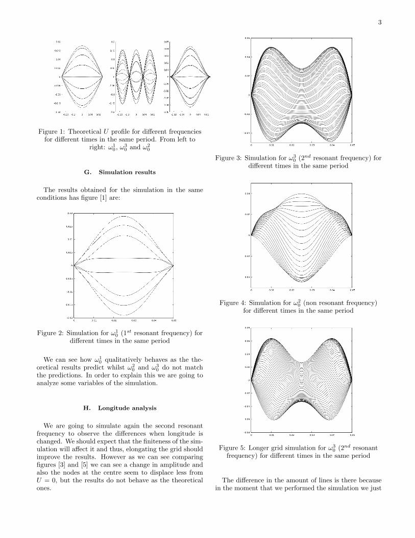
We are going to simulate again the second resonantfrequency to observe the differences when longitude ischanged. We should expect that the finiteness of the sim-ulation will affect it and thus, elongating the grid shouldimprove the results. However as we can see comparingfigures [3] and [5] we can see a change in amplitude andalso the nodes at the centre seem to displace less fromU = 0, but the results do not behave as the theoreticalones.

Figure 3: Simulation for ω30 (2nd resonant frequency) for

different times in the same period

Figure 4: Simulation for ω20 (non resonant frequency)

for different times in the same period

Figure 5: Longer grid simulation for ω30 (2nd resonant

frequency) for different times in the same period

The difference in the amount of lines is there becausein the moment that we performed the simulation we just

4

graphed a different amount of lines, it has nothing to dowith the simulation in itself.

I. Fineness analysis

It is well known that in most cases increasing the fine-ness does not affect the results. However, in this simu-lation the nodes of the graph seem to displace less fromU = 0 as we increase the number of cells in the grid. Butthe results still do not resemble the predictions.

Figure 6: Thin grid simulation for ω30

J. Non-linear case

Just to see how a more complex model would behave insuch simulations, we simulated the non-linear case withα = 0.85 obtaining similar results (figure [7]).

Figure 7: Simulation for ω30 (2nd resonant frequency)

and α = 0.85 for different times in the same period

K. Convergence

In every one of the cases aforementioned, we checkedthat the system reached steady state, comparing how thevelocity profile evolved at the maximum velocity of oscil-lation in each period (in a particular direction). Obtain-ing a graph like [8].

Figure 8: Convergence plot

Normally, we reached steady state after 5 or 6 periods.

CONCLUSIONS

First of all we should say that making such a simulatorwork was not as easy as it may seem. Installing all thedependencies, understanding how to input the model, theparameters and the grid, and then extracting the infor-mation that we can see in the plots was difficult given thelimited documentation available of the software. How-ever, we managed to do it and obtain the results shown.

The simulation results, though coherent between them,do not coincide with the theoretical results at all. Wehave thought of different reasons for why this could hap-pen and reached some conclusions.

Both increasing the separation of the pistons and thethinness of the grid alters a little bit the amplitude andmakes the profiles pass nearer U = 0 at the middle pointbetween the parallel plates as in the theoretical results.However this does not seem to tend to the desired result.Maybe increasing the thinness of the grid a lot more couldend up converging to the theoretical result but it does notlook promising.

There are two main reasons that we think may explainthe obtained results. On one hand, the simulator mightnot be doing what we wanted at all. A thorougher studyand work with the software would have been great andwe could have a better performance of the simulation,though it was not possible with limited time. On theother hand we may have wronged by approximating the

5

boundary conditions of the pistons with the function invelocities.

Finally we would like to that say we have learned a lot

about the scientific method and the trial and error whichcharacterizes it. We would also like to thank L. Ramırez-Piscina for conducting such an interesting project.

REFERENCES

[1] Laura Casanellas Vilageliu. Oscillatory pipe flow of worm-like micellar solutions, PhD Thesis, Physics Dept., UB.

January 2013.[2] L. Ramırez-Piscina via private communication.[3] Alexander Morozov and Saverio E. Spagnolie. Introduction

to Complex Fluids (book)

ANNEX IAdrià Barja Romero and Joan Marco Rimmek

May 2017

IntroductionIn this annex, the most important code files are presented. They define theproperties of the fluid, the configuration of the simulation, the geomentry andmesh used and the initial conditions.

Properties of the fluid constant/

In this folder you can find the dictionary constitutiveProperties.In this file, the properties of the fluid are defined. In the example shown

bellow the properties where defined by: ηP = 64 kgm·s , ηS = 0, ρ = 1050 kg

m3 andλ = 1.9s.

1 /∗−−−−−−−−−−−−−−−−−−−−−−−−−−−−−−−−∗− C++−∗−−−−−−−−−−−−−−−−−−−−−−−−−−−−−−−−−−∗\2 | ========= | |3 | \\ / F ie ld | OpenFOAM: The Open Source CFD Toolbox |4 | \\ / O peration | Version : 4.0 |5 | \\ / A nd | Web: www.OpenFOAM. org |6 | \\/ M anipulation | |7 \∗−−−−−−−−−−−−−−−−−−−−−−−−−−−−−−−−−−−−−−−−−−−−−−−−−−−−−−−−−−−−−−−−−−−−−−−−−−−∗/8 FoamFile9 {

10 version 2.0;11 format asc i i ;12 class dictionary ;13 object constitutiveProperties ;14 }15 // ∗ ∗ ∗ ∗ ∗ ∗ ∗ ∗ ∗ ∗ ∗ ∗ ∗ ∗ ∗ ∗ ∗ ∗ ∗ ∗ ∗ ∗ ∗ ∗ ∗ ∗ ∗ ∗ ∗ ∗ ∗ ∗ ∗ ∗ ∗ ∗ ∗ //1617 parameters18 {19 type Oldroyd−BLog;2021 rho rho [1 −3 0 0 0 0 0] 1050;22 etaS etaS [1 −1 −1 0 0 0 0] 0;23 etaP etaP [1 −1 −1 0 0 0 0] 64;24 lambda lambda [0 0 1 0 0 0 0] 1.9 ;25 uTauCoupling true ;26 }2728 passiveScalarProperties

1

29 {30 solvePassiveScalar of f ;31 D D [ 0 2 −1 0 0 0 0 ] 1e−9;32 }33 // ∗∗∗∗∗∗∗∗∗∗∗∗∗∗∗∗∗∗∗∗∗∗∗∗∗∗∗∗∗∗∗∗∗∗∗∗∗∗∗∗∗∗∗∗∗∗∗∗∗∗∗∗∗∗∗∗∗∗∗∗∗∗∗∗∗∗∗∗∗∗∗∗∗ //

The numbers between brackets define the units of each constant, they cor-respond to [kg m s K mol A cd].

Initial conditions 0/

In this folder there are four files: p, tau, theta and U.We will show the file U since it is the most interesting in our case. The syntax

of the others is very similar in any case.Bellow is the initial condition for an oscillation of amplitude 0.001m and

frequency of 33.76...rad/s.1 /∗−−−−−−−−−−−−−−−−−−−−−−−−−−−−−−−−∗− C++−∗−−−−−−−−−−−−−−−−−−−−−−−−−−−−−−−−−−∗\2 | ========= | |3 | \\ / F ie ld | OpenFOAM: The Open Source CFD Toolbox |4 | \\ / O peration | Version : 4.0 |5 | \\ / A nd | Web: www.OpenFOAM. org |6 | \\/ M anipulation | |7 \∗−−−−−−−−−−−−−−−−−−−−−−−−−−−−−−−−−−−−−−−−−−−−−−−−−−−−−−−−−−−−−−−−−−−−−−−−−−−∗/8 FoamFile9 {

10 version 2.0;11 format asc i i ;12 class volVectorField ;13 object U;14 }15 // ∗ ∗ ∗ ∗ ∗ ∗ ∗ ∗ ∗ ∗ ∗ ∗ ∗ ∗ ∗ ∗ ∗ ∗ ∗ ∗ ∗ ∗ ∗ ∗ ∗ ∗ ∗ ∗ ∗ ∗ ∗ ∗ ∗ ∗ ∗ ∗ ∗ //1617 dimensions [0 1 −1 0 0 0 0 ] ;1819 internalField uniform (0 0 0) ;2021 boundaryField22 {23 in let24 {25 type codedFixedValue ;26 value uniform (0 0 0) ;27 redirectType smoothU;28 code29 //Cosinusoidal30 #{31 const scalar& t = this−>db() . time() . timeOutputValue() ;32 vector Uav(1 , 0 , 0) ;33 vector dirN(1 , 0 , 0) ;34 Uav = ((0.001∗33.760313226149∗Foam: : cos(33.760313226149∗t ) ) ∗ dirN) ;35 operator == (Uav) ;36 #};37 }3839 walls40 {41 type fixedValue ;

2

42 value uniform (0 0 0) ;43 }4445 outlet46 {47 type codedFixedValue ;48 value uniform (0 0 0) ;49 redirectType smoothU;50 code51 //Cosinusoidal52 #{53 const scalar& t = this−>db() . time() . timeOutputValue() ;54 vector Uav(1 , 0 , 0) ;55 vector dirN(1 , 0 , 0) ;56 Uav = ((0.001∗33.760313226149∗Foam: : cos(33.760313226149∗t ) ) ∗ dirN) ;57 operator == (Uav) ;58 #};59 }6061 frontAndBack62 {63 type symmetry;64 }65 }66 // ∗∗∗∗∗∗∗∗∗∗∗∗∗∗∗∗∗∗∗∗∗∗∗∗∗∗∗∗∗∗∗∗∗∗∗∗∗∗∗∗∗∗∗∗∗∗∗∗∗∗∗∗∗∗∗∗∗∗∗∗∗∗∗∗∗∗∗∗∗∗∗∗∗ //

Mesh properties system/

In this folder we can find the file blockMeshDict which dictates the geometryin which the simulation will take place.

1 /∗−−−−−−−−−−−−−−−−−−−−−−−−−−−−−−−−∗− C++−∗−−−−−−−−−−−−−−−−−−−−−−−−−−−−−−−−−−∗\2 | ========= | |3 | \\ / F ie ld | OpenFOAM: The Open Source CFD Toolbox |4 | \\ / O peration | Version : 4.0 |5 | \\ / A nd | Web: www.OpenFOAM. org |6 | \\/ M anipulation | |7 \∗−−−−−−−−−−−−−−−−−−−−−−−−−−−−−−−−−−−−−−−−−−−−−−−−−−−−−−−−−−−−−−−−−−−−−−−−−−−∗/8 FoamFile9 {

10 version 2.0;11 format asc i i ;12 class dictionary ;13 object blockMeshDict ;14 }15 // ∗ ∗ ∗ ∗ ∗ ∗ ∗ ∗ ∗ ∗ ∗ ∗ ∗ ∗ ∗ ∗ ∗ ∗ ∗ ∗ ∗ ∗ ∗ ∗ ∗ ∗ ∗ ∗ ∗ ∗ ∗ ∗ ∗ ∗ ∗ ∗ ∗ //1617 convertToMeters 0.1 ;1819 vertices20 (21 (0 −0.25 −0.25)22 (3 −0.25 −0.25)23 (3 0.25 −0.25)24 (0 0.25 −0.25)25 (0 −0.25 0.25)26 (3 −0.25 0.25)27 (3 0.25 0.25)28 (0 0.25 0.25)29 ) ;30

3

31 blocks32 (33 hex (0 1 2 3 4 5 6 7) (50 60 12) simpleGrading (1 1 1) //034 ) ;3536 edges37 (38 ) ;3940 boundary41 (42 in let43 {44 type patch ;45 faces46 (47 (0 4 7 3)48 ) ;49 }5051 outlet52 {53 type patch ;54 faces55 (56 (1 2 6 5)57 ) ;58 }5960 walls61 {62 type wall ;63 faces64 (65 (2 3 7 6)66 (0 1 5 4)67 ) ;68 }6970 frontAndBack71 {72 type symmetry;73 faces74 (75 (4 5 6 7)76 (1 0 3 2)77 ) ;78 }79 ) ;8081 mergePatchPairs82 (83 ) ;84 // ∗∗∗∗∗∗∗∗∗∗∗∗∗∗∗∗∗∗∗∗∗∗∗∗∗∗∗∗∗∗∗∗∗∗∗∗∗∗∗∗∗∗∗∗∗∗∗∗∗∗∗∗∗∗∗∗∗∗∗∗∗∗∗∗∗∗∗∗∗∗∗∗∗ //

The option convertToMeters 0.1 multiplies each dimension by 0.1. There-fore, our parallel planes have a separation of 0.025m and the distance betweenthe two pistons is of 0.3m.

4

Simulation parameters system/

Also, in folder system we can find the file controlDict which dictates theparameters of the the simulation in itself. Here you can configure the initial andfinal times, the time-step and personalized functions in order to retrieve datafrom the raw files.

1 /∗−−−−−−−−−−−−−−−−−−−−−−−−−−−−−−−−∗− C++−∗−−−−−−−−−−−−−−−−−−−−−−−−−−−−−−−−−−∗\2 | ========= | |3 | \\ / F ie ld | OpenFOAM: The Open Source CFD Toolbox |4 | \\ / O peration | Version : 4.0 |5 | \\ / A nd | Web: www.OpenFOAM. org |6 | \\/ M anipulation | |7 \∗−−−−−−−−−−−−−−−−−−−−−−−−−−−−−−−−−−−−−−−−−−−−−−−−−−−−−−−−−−−−−−−−−−−−−−−−−−−∗/8 FoamFile9 {

10 version 2.0;11 format asc i i ;12 class dictionary ;13 object controlDict ;14 }15 // ∗ ∗ ∗ ∗ ∗ ∗ ∗ ∗ ∗ ∗ ∗ ∗ ∗ ∗ ∗ ∗ ∗ ∗ ∗ ∗ ∗ ∗ ∗ ∗ ∗ ∗ ∗ ∗ ∗ ∗ ∗ ∗ ∗ ∗ ∗ ∗ ∗ //1617 application rheoFoam;1819 startFrom startTime ;20 startTime 0;2122 stopAt endTime;23 endTime 0.95;2425 deltaT 0.0002;2627 writeControl timeStep ;28 writeInterval 1;29 purgeWrite 0;30 writeFormat asc i i ;31 writePrecision 12;32 writeCompression compressed ;33 timeFormat general ;34 timePrecision 10;35 graphFormat raw;36 runTimeModifiable no ;37 adjustTimeStep of f ;38 maxCo 0.1;39 maxDeltaT 0.01;4041 functions42 {43 #includeFunc singleGraph44 }45 // ∗∗∗∗∗∗∗∗∗∗∗∗∗∗∗∗∗∗∗∗∗∗∗∗∗∗∗∗∗∗∗∗∗∗∗∗∗∗∗∗∗∗∗∗∗∗∗∗∗∗∗∗∗∗∗∗∗∗∗∗∗∗∗∗∗∗∗∗∗∗∗∗∗ //

In this case we start the simulation at time 0s and end it at time 0.95s usinga time-step of 0.0002s. Moreover, the function singleGraph can be found inanother file in the same folder, and is the one that retrieves the data of thevelocity profiles:

5

1 /∗−−−−−−−−−−−−−−−−−−−−−−−−−−−−−−−−∗− C++−∗−−−−−−−−−−−−−−−−−−−−−−−−−−−−−−−−−−∗\2 ========= |3 \\ / F ield | OpenFOAM: The Open Source CFD Toolbox4 \\ / O peration |5 \\ / A nd | Web: www.OpenFOAM. org6 \\/ M anipulation |7 −−−−−−−−−−−−−−−−−−−−−−−−−−−−−−−−−−−−−−−−−−−−−−−−−−−−−−−−−−−−−−−−−−−−−−−−−−−−−−−8 Description9 Writes graph data for specif ied f i e l d s along a line , speci f ied by start

10 and end points .11 \∗−−−−−−−−−−−−−−−−−−−−−−−−−−−−−−−−−−−−−−−−−−−−−−−−−−−−−−−−−−−−−−−−−−−−−−−−−−−∗/1213 start (0.15 −0.025 0) ;14 end (0.15 0.025 0) ;15 f i e l d s (U) ;1617 // Sampling and I/O settings18 #includeEtc ”caseDicts/postProcessing/graphs/sampleDict . cfg”1920 // Override settings here , e . g .21 // setConfig { type midPoint ; }2223 // Must be last entry24 #includeEtc ”caseDicts/postProcessing/graphs/graph . cfg”25 // ∗∗∗∗∗∗∗∗∗∗∗∗∗∗∗∗∗∗∗∗∗∗∗∗∗∗∗∗∗∗∗∗∗∗∗∗∗∗∗∗∗∗∗∗∗∗∗∗∗∗∗∗∗∗∗∗∗∗∗∗∗∗∗∗∗∗∗∗∗∗∗∗∗ //

Although there are many more files in each OpenFOAM case, those wherethe most important and the only ones we had to modify to make one simulationor another.

6

ANNEX IIAdrià Barja Romero and Joan Marco Rimmek

May 2017

IntroductionIn this annex images and plots obtained from the simulation are present.

GridThe grid we used in our simulations, which is 0.3m long and has 60 divisions inthe x axis, is 0.05m long and has 60 divisions in the y axis and is 0.05m longand has 16 divisions in the z axis.

Figure 1: Grid used in the simulations

1

Post-processed simulations

Figure 2: Image of the post-processed simulation at the first moments of thesimulation

Figure 3: Image of the post-processed simulation at a change of direction in thevelocity

2