vision 3d artificielle session 1: projective geometry

3D Computer VisionSession 1: Projective geometry, camera matrix,

panorama

Pascal [email protected]

IMAGINE, École des Ponts ParisTech

This work is licensed under the Creative Commons Attribution 4.0International License. To view a copy of this license, visit

http://creativecommons.org/licenses/by/4.0/.

mailto:[email protected]

http://creativecommons.org/licenses/by/4.0/

Contents

Pinhole camera model

Projective geometry

Homographies

Panorama

Internal calibration

Optimization techniques

Conclusion

Practical session/Home assignment

The �pinhole� camera model

Projection (Source: Wikipedia)x

y

z

m

M

C

camera center

image plane

image point

World point

ModelThe�pinhole� camera (French: sténopé):

I Ideal model with an aperture reduced to a single point.

I No account for blur of out of focus objects, nor for the lensgeometric distortion.

Central projection in camera coordinate frame

I Rays from C are the same: ~Cm = λ ~CM

I In the camera coordinate frame CXYZ :xyf

= λ

XYZ

I Thus λ = f /Z and (

xy

)= f

(X/ZY /Z

)I In pixel coordinates:(

uv

)=

(αx + cxαy + cy

)=

((αf )X/Z + cx(αf )Y /Z + cy

)I αf : focal length in pixels, (cx , cy ): position of principal point

P in pixels.

Contents


Projective geometry

Homographies

Panorama



Conclusion


Projective plane

I We identify two points of R3 on the same ray from the originthrough the equivalence relation:

R : xRy⇔ ∃λ 6= 0 : x = λy

I Projective plane: P2 = (R3 \ O)/RI Point

(x y z

)=(x/z y/z 1

)if z 6= 0.

I The point(x/ε y/ε 1

)=(x y ε

)is a point �far away� in

the direction of the line of slope y/x . The limit value(x y 0

)is the in�nite point in this direction.

I Given a plane of R3 through O, its equation isaX + bY + cZ = 0. It corresponds to a line in P2 representedin homogeneous coordinates by

(a b c

). Its equation is:(

a b c) (

X Y Z)>

= 0.

Projective plane

I Line through points x1 and x2:

` = x1 × x2 since (x1 × x2)>xi = |x1 x2 xi| = 0

I Intersection of two lines `1 and `2:

x = `1 × `2 since `>i (`1 × `2) = |`i `1 `2| = 0

I Line at in�nity:

`∞ =

001

since `>∞

xy0

= 0

I Intersection of two �parallel� lines: abc1

× a

bc2

= (c2 − c1)

b−a0

∈ `∞

Calibration matrix

I Let us get back to the projection equation:(uv

)=

(fX/Z + cxfY /Z + cy

)=

1

Z

(fX + cxZfY + cyZ

)(replacing αf by f )

I We rewrite:

Z

uv1

:= x =

f cxf cy

1

XYZ

I The 3D point being expressed in another orthonormal

coordinate frame:

x =

f cxf cy

1

(R T)

XYZ1

Calibration matrixI The (internal) calibration matrix (3× 3) is:

K =

f cxf cy

1

I The projection matrix (3× 4) is:

P = K(R T

)I If pixels are trapezoids, we can generalize K :

K =

fx s cxfy cy

1

(with s = −fx cotan θ)

Theorem

Let P be a 3× 4 matrix whose left 3× 3 sub-matrix is invertible.

There is a unique decomposition P = K(R T

).

Proof: Gram-Schmidt on rows of left sub-matrix of P starting fromlast row (RQ decomposition), then T = K−1P4.

Projective plane (perspective e�ect)

I Lines parallel in space project to a line bundle (set of linesparallel or concurrent). Let d be a �xed direction vector:

K (X+ λd) = KX+ λKd

`X = (KX)× (Kd)

∀X, `>Xv = 0 for v := Kd

I v is the vanishing point of lines of direction d.

I If v1 = Kd1 and v2 = Kd2 are vp of �horizontal� lines,another set of horizontal lines has direction αd1 + βd2, henceits vp αv1 + βv2, which belongs to line v1 × v2, the �horizon�.

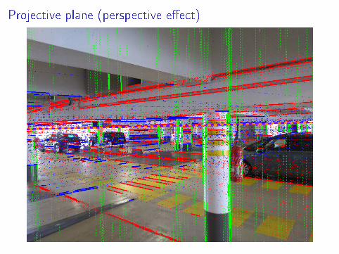
Projective plane (perspective e�ect)

Contents


Projective geometry

Homographies

Panorama



Conclusion


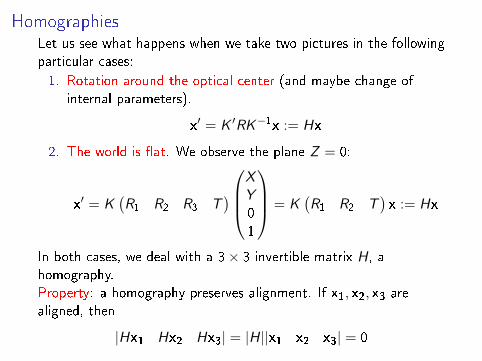
HomographiesLet us see what happens when we take two pictures in the followingparticular cases:

1. Rotation around the optical center (and maybe change ofinternal parameters).

x′ = K ′RK−1x := Hx

2. The world is �at. We observe the plane Z = 0:

x′ = K(R1 R2 R3 T

)XY01

= K(R1 R2 T

)x := Hx

In both cases, we deal with a 3× 3 invertible matrix H, ahomography.Property: a homography preserves alignment. If x1, x2, x3 arealigned, then

|Hx1 Hx2 Hx3| = |H||x1 x2 x3| = 0

HomographiesType Matrix Invariants

Rigid (Rot.+Trans.) H =

c −s txs c ty0 0 1

(c2 + s2 = 1)angles,distances

Similarity H =

c −s txs c ty0 0 1

angles,ratio ofdistances

A�ne H =

a b txc d ty0 0 1

parallelism

Homography H invertible

cross-ratio of4 alignedpoints

Given 4 aligned points A, B , C , D, their cross-ratio is:

(A,B;C ,D) =AC

BC:AD

BD

Homographies: estimation from point correspondencesTheorem Let e1, · · · , ed+1, f1, · · · , fd+1 ∈ Rd such that any dvectors ei (resp. fi ) are linearly independent. Then there are (up toscale) a unique isomorphism H and a unique set of scalars λi 6= 0so that ∀i ,Hei = λi fi .

1. Analysis: writing ed+1 =∑d

i=1 µiei and fd+1 =∑d

i=1 νi fi ,

d∑i=1

νiλd+1fi = λd+1fd+1 = Hed+1 =d∑

i=1

µiλi fi

so that ∀i = 1, . . . , d : µiλi = νiλd+1.

2. ∀i , µi 6= 0 and νi 6= 0, since µi = 0⇒ {ej}j 6=i are linearlydependent.

3. Therefore we get λi =νiµiλd+1.

4. Synthesis: �x λd+1 = 1 and ∀i : λi = νiµi6= 0.

5. There is a unique H mapping basis {ei}i=1,...,d to basis{λi fi}i=1,...,d

Application: given n + 2 pairs (xi, x′i) ∈ Pn, there is a unique

homography mapping xi to x′i.

Contents


Projective geometry

Homographies

Panorama



Conclusion


Panorama constructionI We stitch together images by correcting homographies. This

assumes that the scene is �at or that we are rotating thecamera.

I Homography estimation:

λx′ = Hx⇒ x′ × (Hx) = 0,

which amounts to 2 independent linear equations percorrespondence (x, x′).

I 4 correspondences are enough to estimate H (but more can beused to estimate through mean squares minimization).

Panorama from 14 photos

Algebraic error minimization

I x′i× (Hxi) = 0 is a system of three linear equations in H.

I We gather the unkwown coe�cients of H in a vector of 9 rows

h =(H11 H12 . . . H33

)>I We write the equations as Aih = 0 with

Ai =

(xi yi 1 0 0 0 −x ′i xi −x ′i yi −x ′i0 0 0 xi yi 1 −y ′

i xi −y ′i yi −y ′

i

−xiy ′i −yiy ′

i −y ′i x ′i xi x ′i yi x ′i 0 0 0

)

I We can discard the third line and stack the di�erent Ai in A.

I h is a vector of the kernel of A (8× 9 matrix)

I We can also suppose H3,3 = h9 = 1 and solve

A:,1:8h1:8 = −A:,9

Geometric errorI When we have more than 4 correspondences, we minimize the

algebraic error

ε =∑i

‖x′i × (Hxi)‖2,

but it has no geometric meaning.I A more signi�cant error is geometric:

Image 1 Image 2d’

d

H

H−1

xx’

Hx

−1H x’

I Either d′2 = d(x′,Hx)2 (transfer error) or

d2 + d′2 = d(x,H−1x′)2 + d(x′,Hx)2(Symmetric transfer error)

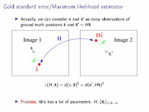
Gold standard error/Maximum likelihood estimator

I Actually, we can consider x and x′ as noisy observations ofground truth positions x̂ and x̂′ = H x̂.

Image 1 Image 2d’

d

xx’

HHx

^x

^

ε(H, x̂) = d(x , x̂)2 + d(x′,H x̂)2

I Problem: this has a lot of parameters: H, {x̂i}i=1...n

Sampson error

I A method that linearizes the dependency on x̂ in the goldstandard error so as to eliminate these unknowns.

0 = ε(H, x̂) = ε(H, x) + J (̂x− x) with J =∂ε

∂x(H, x)

I Find x̂ minimizing ‖x− x̂‖2 subject to J(x− x̂) = ε

I Solution: x− x̂ = J>(JJ>)−1ε and thus:

‖x− x̂‖2 = ε>(JJ>)−1ε (1)

I Here, εi = Aih = x′i× (Hxi) is a 3-vector.

I For each i , there are 4 variables (xi, x′i), so J is 3× 4.

I This is almost the algebraic error ε>ε but with adapted scalarproduct.

I The resolution, through iterative method, must be initializedwith the algebraic minimization.

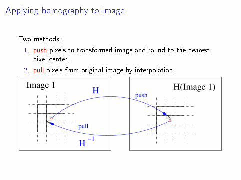
Applying homography to image

Two methods:

1. push pixels to transformed image and round to the nearestpixel center.

2. pull pixels from original image by interpolation.

H(Image 1)Image 1H

H−1

push

pull

Contents


Projective geometry

Homographies

Panorama



Conclusion


Camera calibration by resection[R.Y. Tsai,An e�cient and accurate camera calibration technique

for 3D machine vision, CVPR'86] We estimate the camera internalparameters from a known rig, composed of 3D points whosecoordinates are known.

I We have points Xi and their projection xi in an image.

I In homogeneous coordinates: xi = PXi or the 3 equations (butonly 2 of them are independent)

xi × (PXi) = 0

I Linear system in unknown P . There are 12 parameters in P ,we need 6 points in general (actually only 5.5).

I Decomposition of P allows �nding K .

Restriction: The 6 points cannot be on a plane,otherwise we have a degenerate situation; in thatcase, 4 points de�ne the homography and the twoextra points yield no additional constraint.

Calibration with planar rig[Z. Zhang A �exible new technique for camera calibration 2000]I Problem: One picture is not enough to �nd K .I Solution: Several snapshots are used.I For each one, we determine the homography H between the

rig and the image.I The homography being computed with an arbitrary

multiplicative factor, we write

λH = K(R1 R2 T

)I We rewrite:

λK−1H = λ(K−1H1 K−1H2 K−1H3

)=(R1 R2 T

)I 2 equations expressing orthonormality of R1 and R2:

H>1 (K−>K−1)H1 = H>2 (K−>K−1)H2

H>1 (K−>K−1)H2 = 0

I With 3 views, we have 6 equations for the 5 parameters ofK−>K−1; then Cholesky decomposition.

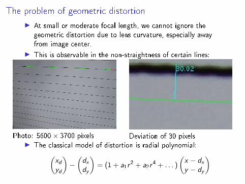
The problem of geometric distortion

I At small or moderate focal length, we cannot ignore thegeometric distortion due to lens curvature, especially awayfrom image center.

I This is observable in the non-straightness of certain lines:

Photo: 5600× 3700 pixels Deviation of 30 pixelsI The classical model of distortion is radial polynomial:(

xdyd

)−(dxdy

)= (1+ a1r

2 + a2r4 + . . . )

(x − dxy − dy

)

Estimation of geometric distortion

I If we integrate distortion coe�cients as unknowns, there is nomore closed formula estimating K .

I We have a non-linear minimization problem, which can besolved by an iterative method.

I To initialize the minimization, we assume no distortion(a1 = a2 = 0) and estimate K with the previous linearprocedure.

Contents


Projective geometry

Homographies

Panorama



Conclusion


Linear least squares problemI For example, when we have more than 4 point

correspondences in homography estimation:

Am×8h = Bm m ≥ 8

I In the case of an overdetermined linear system, we minimize

ε(X) = ‖AX− B‖2 = ‖f (X)‖2

I The gradient of ε can be easily computed:

∇ε(X) = 2(A>AX− A>B)

I The solution is obtained by equating the gradient to 0:

X = (A>A)−1A>B

I Remark 1: this is correct only if A>A is invertible, that is Ahas full rank.

I Remark 2: if A is square, it is the standard solution X = A−1BI Remark 3: A(−1) = (A>A)−1A> is called the pseudo-inverse of

A, because A(−1)A = In.

Non-linear least squares problem

I We would like to solve as best we can f (X) = 0 with fnon-linear. We thus minimize

ε(X) = ‖f (X)‖2

I Let us compute the gradient of ε:

∇ε(X) = 2J>f (X) with Jij =∂fi∂xj

I Gradient descent: we iterate until convergence

4X = −αJ>f (X), α > 0

I When we are close to the minimum, a faster convergence isobtained by Newton's method:

ε(X0) ∼ ε(X) +∇ε(X)>(4X) + (4X)>(∇2ε)(4X)/2

and minimum is for 4X = −(∇2ε)−1∇ε

Levenberg-Marquardt algorithm

I This is a mix of gradient descent and quasi-Newton method(quasi since we do not compute explictly the Hessian matrix,but approximate it).

I The gradient of ε is

∇ε(X) = 2J>f (X)

so the Hessian matrix of ε is composed of sums of two terms:1. Product of first derivatives of f .2. Product of f and second derivatives of f .

I The idea is to ignore the second terms, as they should be smallwhen we are close to the minimum (f ∼ 0). The Hessian isthus approximated by

H = 2J>J

I Levenberg-Marquardt iteration:

4X = −(J>J + λI )−1J>f (X), λ > 0

Levenberg-Marquardt algorithm

I Principle: gradient descent when we are far from the solution(λ large) and Newton's step when we are close (λ small).

1. Start from initial X and λ = 10−3.

2. Compute

4X = −(J>J + λI )−1J>f (X), λ > 0

3. Compare ε(X+4X) and ε(X):3a If ε(X +4X) ∼ ε(X), finish.3b If ε(X +4X) < ε(X),

X← X +4X λ← λ/10

3c If ε(X +4X) > ε(X), λ← 10λ

4. Go to step 2.

Example of distortion correction

Results of Zhang:

Snapshot 1 Snapshot 2

Example of distortion correction

Results of Zhang:

Corrected image 1 Corrected image 2

Contents


Projective geometry

Homographies

Panorama



Conclusion


Conclusion

I Camera matrix K (3× 3) depends only on internal parametersof the camera.

I Projection matrix P (3× 4) depends on K andposition/orientation.

I Homogeneous coordinates are convenient as they linearize theequations.

I A homography between two images arises when the observedscene is �at or the principal point is �xed.

I 4 or more correspondences are enough to estimate ahomography (in general)

References

Hartley & Zisserman (2004)

I Chapter 2: Projective Geometry andTransformations of 2D

I Chapter 4: Estimation�2D ProjectiveTransformations

I Chapter 6: Camera Models

I Chapter 7: Computation of the Camera Matrix P

Semple & Kneebone (1962)

I Chapter IV: Projective Geometry of TwoDimensions

I Appendix: Two Basic Algebraic Theorems

Contents


Projective geometry

Homographies

Panorama



Conclusion


Practical session: panorama construction

Objective: the user clicks 4 or more corresponding points in left andright images. After a right button click, the program computes thehomography and shows the resulting panorama in a new window.

I Install Imagine++(http://imagine.enpc.fr/~monasse/Imagine++/) on yourmachine.

I Let the user click the matching points.

I Build the linear system to solve Ax = b and �nd x .

I Compute the bounding box of the panorama.

I Stitch the images: on overlapping area, take the average ofcolors at corresponding pixels in both images.

Useful Imagine++ types/functions: Matrix, Vector, Image,anyGetMouse, linSolve

http://imagine.enpc.fr/~monasse/Imagine++/

vision 3d artificielle session 1: projective geometry

Documents