vision - nrcmec.org master.pdf · vision: to emerge as a destination for higher education by...

Humanities & Sciences Engineering Physics Lab

Narsimha Reddy Engineering College Page -1

Vision:

To emerge as a destination for higher education by

transforming learners into achievers by creating, encouraging

and thus building a supportive academic environment.

Mission:

To impart Quality Technical Education and to undertake

Research and Development with a focus on application and

innovation which offers an appropriate solution to the

emerging societal needs by making the students globally

competitive, morally valuable and socially responsible citizens.



INSTRUCTIONS FOR LABORATORY

1) The objective of the laboratory is learning. The experiments are designed to

illustrate phenomena in different areas of Physics and to expose you to

measuring instruments. Conduct the experiments with interest and an attitude

of learning.

2) You need to come well prepared for the experiment

3) Work quietly and carefully (the whole purpose of experimentation is to make

reliable measurements!) and equally share the work with your partners.

4) Be honest in recording and representing your data. Never make up readings or

doctor them to get a better fit for a graph. If a particular reading appears wrong

repeat the measurement carefully. In any event all the data recorded in the

tables have to be faithfully displayed on the graph.

5) All presentations of data, tables and graphs calculations should be neatly and

carefully done.

6) Bring necessary graph papers for each of experiment. Learn to optimize on

usage of graph papers.

7) Graphs should be neatly drawn with pencil. Always label graphs and the axes

and display units.

8) If you finish early, spend the remaining time to complete the calculations and

drawing graphs. Come equipped with calculator, scales, pencils etc.

9) Do not fiddle idly with apparatus. Handle instruments with care. Report any

breakage to the Instructor. Return all the equipment you have signed out for

the purpose of your experiment.



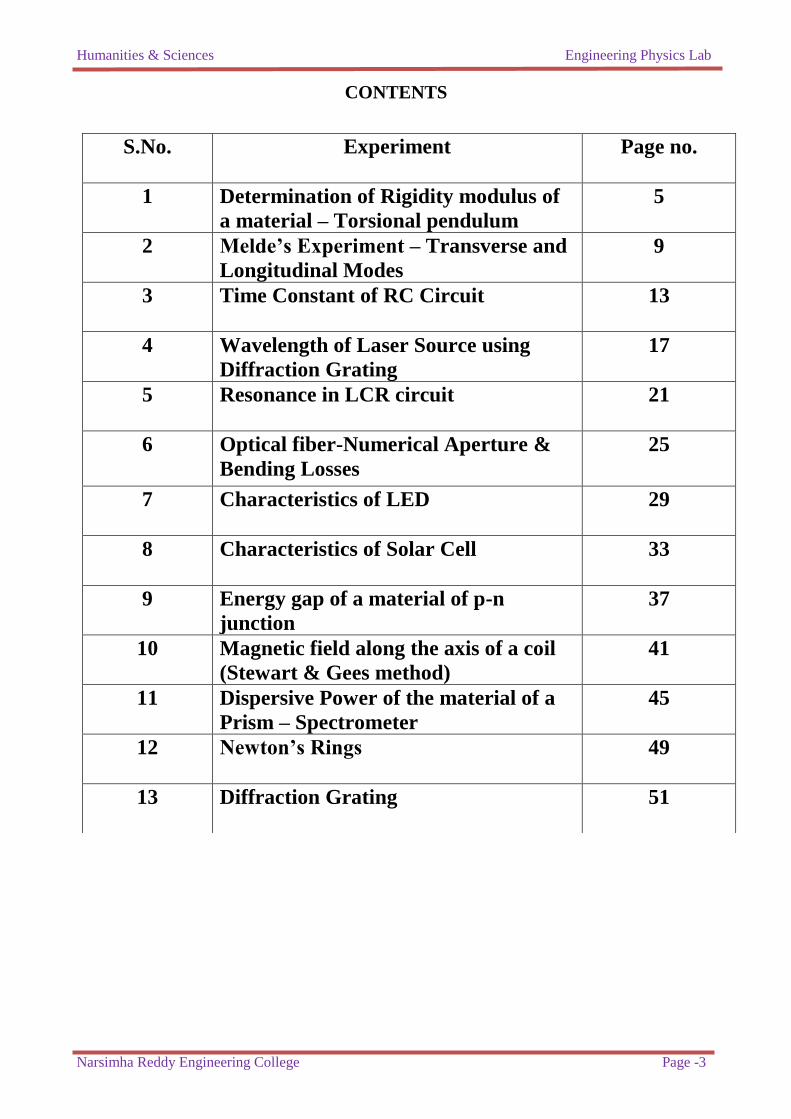
CONTENTS

S.No. Experiment Page no.

1 Determination of Rigidity modulus of

a material – Torsional pendulum

5

2 Melde’s Experiment – Transverse and

Longitudinal Modes

9

3 Time Constant of RC Circuit 13

4 Wavelength of Laser Source using

Diffraction Grating

17

5 Resonance in LCR circuit 21

6 Optical fiber-Numerical Aperture &

Bending Losses

25

7 Characteristics of LED 29

8 Characteristics of Solar Cell 33

9 Energy gap of a material of p-n

junction

37

10 Magnetic field along the axis of a coil

(Stewart & Gees method)

41

11 Dispersive Power of the material of a

Prism – Spectrometer

45

12 Newton’s Rings

49

13 Diffraction Grating 51



1. Torsional Pendulum

AIM:

To determine the rigidity modulus (η) of the given wire using a Torsional

pendulum.

Apparatus:

Torsional Pendulum, steel wire, stopwatch, meter scale, screw gauge, Vernier

calipers.

Principle:

Rigidity Modulus: η =

)dynes/cm

2

M - Mass of the disc.(gm)

R - Radius of the disc.(cm)

a - Radius of the wire.(cm)

l - Length of the pendulum.(cm)

T - Time period.(sec)

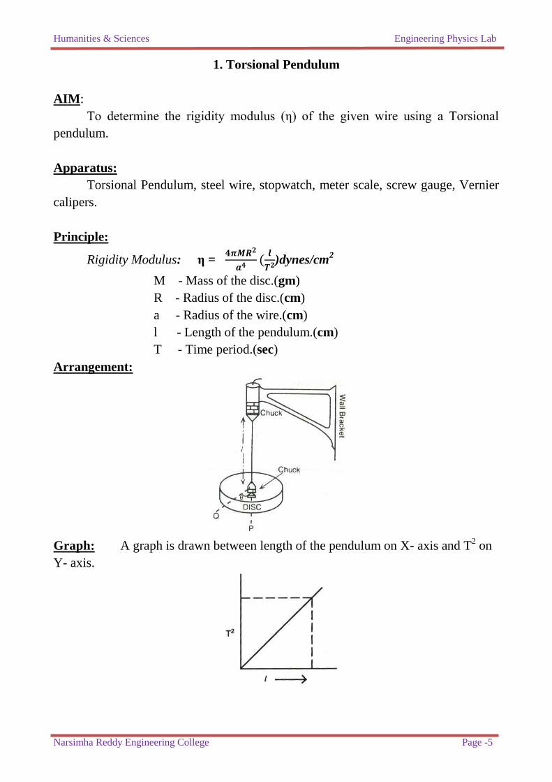
Arrangement:

Graph: A graph is drawn between length of the pendulum on X- axis and T

2 on

Y- axis.



Procedure:

The circular metal disc is suspended by steel wire as shown in the fig. The

length of the wire between the chuck nuts is adjusted to 100cm.A small mark is made

on the curved edge of the disc. The disc is set to oscillate by slow by turning the disc

through a small angle. There should be no lateral movement of the disc.

When the disc is oscillating the time taken for 20 oscillations is noted with the

help of a stop watch and recorded in the observation table as trial1. This procedure is

repeated for the same length and noted as trial2 in the observation table and mean

value is obtained from the trail1&trail2, calculate the time period(T).The above

procedure is repeated for the lengths 90,80,70&60cm and noted in the observation

table and time period(T) is calculated ie. Time for one oscillation.

The radius of the wire (a) is noted with the help of the screw gauge and

readings are recorded in the observation table and mean radius of the wire (a) is

calculated. Similarly the radius of disc is noted with the help of vernier calipers and

recorded in the observation table and mean radius of the disc is calculated.

A graph is drawn between the „l‟ on the x-axis and T2 on the y-axis.

value is

calculated from the graph .The rigidity modulus (η) is calculated by substituting the

observations in the formula.

Observations:

Mass of the disc (M) = 690 gms

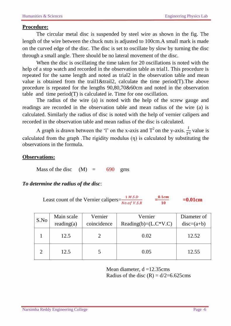
To determine the radius of the disc:

Least count of the Vernier calipers=

=

=0.01cm

S.No Main scale

reading(a)

Vernier

coincidence

Vernier

Reading(b)=(L.C*V.C)

Diameter of

disc=(a+b)

1 12.5 2 0.02 12.52

2 12.5 5 0.05 12.55

Mean diameter, d =12.35cms

Radius of the disc (R) = d/2=6.625cms



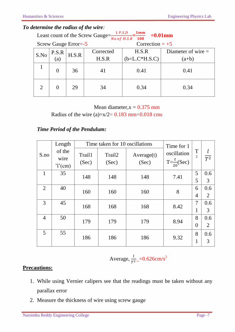
To determine the radius of the wire:

Least count of the Screw Gauge=

=

=0.01mm

Screw Gauge Error=-5 Correction = +5

S.No P.S.R

(a) H.S.R

Corrected

H.S.R

H.S.R

(b=L.C*H.S.C)

Diameter of wire =

(a+b)

1

0 36 41 0.41 0.41

2 0 29 34 0.34 0.34

Mean diameter,x = 0.375 mm

Radius of the wire (a)=x/2= 0.183 mm=0.018 cms

Time Period of the Pendulum:

S.no

Length

of the

wire

‟l‟(cm)

Time taken for 10 oscillations Time for 1

oscillation

T=

(Sec)

T2

Trail1

(Sec)

Trail2

(Sec)

Average(t)

(Sec)

1

35 148 148 148 7.41

5

5

0.6

3

2

40

160 160 160 8

6

4

0.6

2

3

45

168 168 168 8.42

7

1

0.6

3

4

50

179 179 179 8.94

8

0

0.6

2

5 55 186 186 186 9.32

8

1

0.6

3

Average,

_=0.626cm/s

2

Precautions:

1. While using Vernier calipers see that the readings must be taken without any

parallax error

2. Measure the thickness of wire using screw gauge



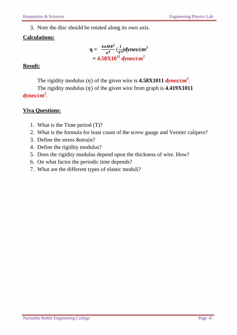
3. Note the disc should be rotated along its own axis.

Calculations:

η =

)dynes/cm

2

= 4.58X1011

dynes/cm2

Result:

The rigidity modulus ( of the given wire is 4.58X1011 dynes/cm2.

The rigidity modulus ( of the given wire from graph is 4.419X1011

dynes/cm2.

Viva Questions:

1. What is the Time period (T)?

2. What is the formula for least count of the screw gauge and Vernier calipers?

3. Define the stress &strain?

4. Define the rigidity modulus?

5. Does the rigidity modulus depend upon the thickness of wire. How?

6. On what factor the periodic time depends?

7. What are the different types of elastic moduli?



2. MELDE’S EXPERIMENT

AIM:

To determine the frequency of a vibrating bar (or) tuning fork using Melde‟s

arrangement.

Apparatus:

Melde‟s arrangement, connecting wires, meter scale, thread, weight box,

power supply.

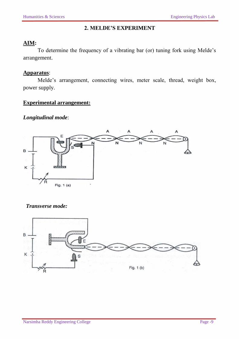
Experimental arrangement:

Longitudinal mode:

Transverse mode:



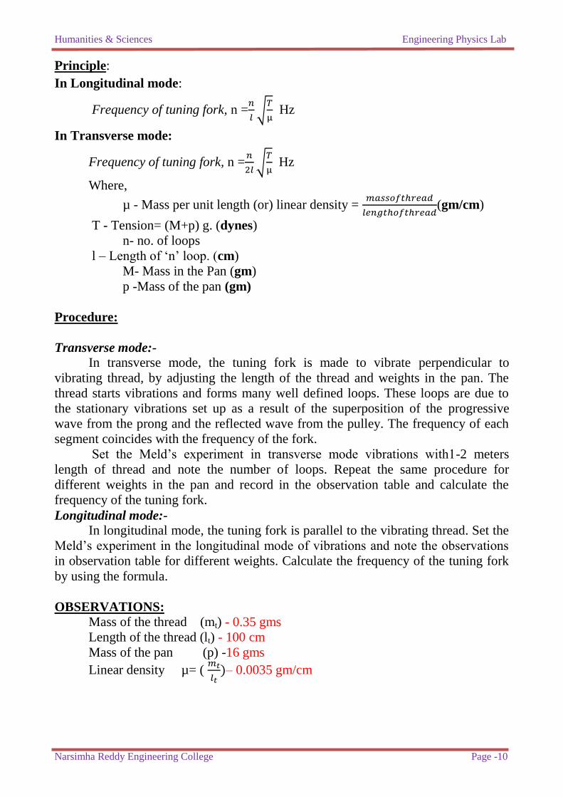
Principle:

In Longitudinal mode:

Frequency of tuning fork, n =

√

Hz

In Transverse mode:

Frequency of tuning fork, n =

√

Hz

Where,

µ - Mass per unit length (or) linear density =

(gm/cm)

T - Tension= (M+p) g. (dynes)

n- no. of loops

l – Length of „n‟ loop. (cm)

M- Mass in the Pan (gm)

p -Mass of the pan (gm)

Procedure:

Transverse mode:-

In transverse mode, the tuning fork is made to vibrate perpendicular to

vibrating thread, by adjusting the length of the thread and weights in the pan. The

thread starts vibrations and forms many well defined loops. These loops are due to

the stationary vibrations set up as a result of the superposition of the progressive

wave from the prong and the reflected wave from the pulley. The frequency of each

segment coincides with the frequency of the fork.

Set the Meld‟s experiment in transverse mode vibrations with1-2 meters

length of thread and note the number of loops. Repeat the same procedure for

different weights in the pan and record in the observation table and calculate the

frequency of the tuning fork.

Longitudinal mode:-

In longitudinal mode, the tuning fork is parallel to the vibrating thread. Set the

Meld‟s experiment in the longitudinal mode of vibrations and note the observations

in observation table for different weights. Calculate the frequency of the tuning fork

by using the formula.

OBSERVATIONS:

Mass of the thread (mt) - 0.35 gms

Length of the thread (lt) - 100 cm

Mass of the pan (p) -16 gms

Linear density µ= (

– 0.0035 gm/cm



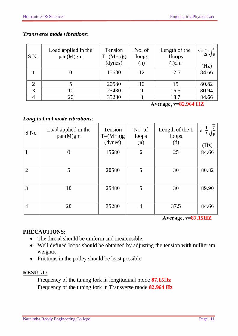
Transverse mode vibrations:

S.No

Load applied in the

pan(M)gm

Tension

T=(M+p)g

(dynes)

No. of

loops

(n)

Length of the

1loops

(l)cm

ν=

√

(Hz)

1 0 15680 12 12.5 84.66

2 5 20580 10 15 80.82

3 10 25480 9 16.6 80.94

4 20 35280 8 18.7 84.66

Average, ν=82.964 HZ

Longitudinal mode vibrations:

S.No

Load applied in the

pan(M)gm

Tension

T=(M+p)g

(dynes)

No. of

loops

(n)

Length of the 1

loops

(d)

ν=

√

(Hz)

1 0 15680 6

25

84.66

2 5 20580 5 30 80.82

3 10 25480 5 30 89.90

4 20 35280 4 37.5 84.66

Average, ν=87.15HZ

PRECAUTIONS:

The thread should be uniform and inextensible.

Well defined loops should be obtained by adjusting the tension with milligram

weights.

Frictions in the pulley should be least possible

RESULT:

Frequency of the tuning fork in longitudinal mode 87.15Hz

Frequency of the tuning fork in Transverse mode 82.964 Hz



Viva Questions:

1. What types of waves are produced in a fork when it is excited?

2. What are a transverse wave and a longitudinal wave?

3. What is a stationary wave?

4. What are beats?

5. What are nodes and antinodes?

6. What is effect of temp in the frequency of the tuning fork?

7. Define frequency and resonance?



3. R.C. CIRCUIT

Aim:

To study the charging and discharging of voltage in a circuit containing

resistance and capacitor and compare the experimental RC time constant with

theoretical RC time constant.

Apparatus:

RC trainer kit, connecting probes, split watch.

Principle:

The charging voltage across the capacitor is given

V= (1 – e -t/RC

)

The discharging voltage across the capacitor is given

V= - e -t/RC

When t=RC then V=0.36 Vο

Where

t – Time constant (sec)

R – Resistance (ohms)

C – Capacitance (farads)

Vο- Max Voltage (volts)

Formula:

Time constant of RC circuit t =RC. (Sec)

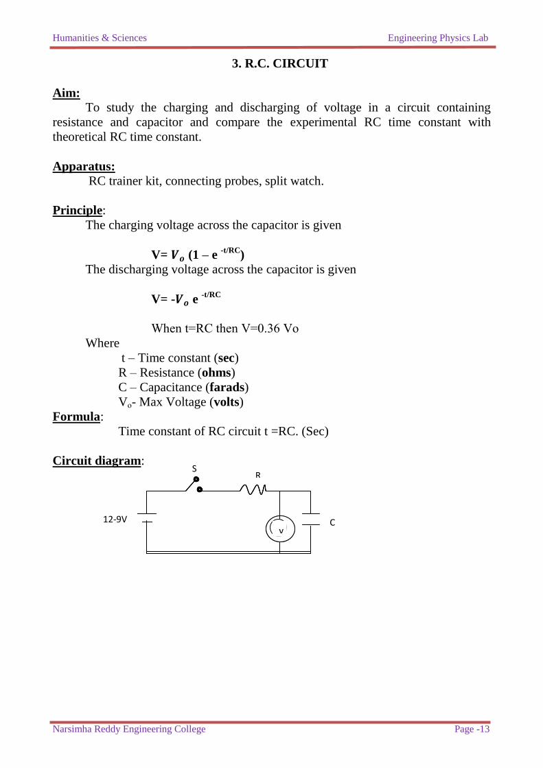
Circuit diagram:

v

R S

12-9V v

R S

12-9V v

C



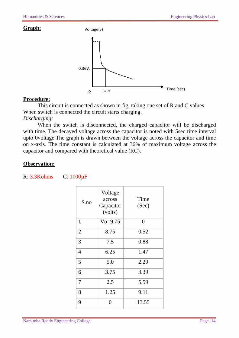
Graph:

Procedure:

This circuit is connected as shown in fig, taking one set of R and C values.

When switch is connected the circuit starts charging.

Discharging:

When the switch is disconnected, the charged capacitor will be discharged

with time. The decayed voltage across the capacitor is noted with 5sec time interval

upto 0voltage.The graph is drawn between the voltage across the capacitor and time

on x-axis. The time constant is calculated at 36% of maximum voltage across the

capacitor and compared with theoretical value (RC).

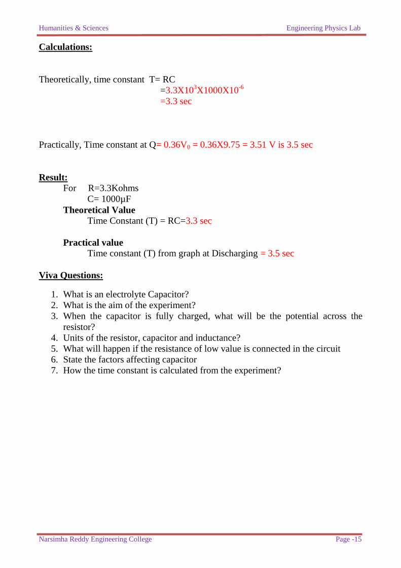
Observation:

R: 3.3Kohms C: 1000µF

S.no

Voltage

across

Capacitor

(volts)

Time

(Sec)

1 Vo=9.75 0

2 8.75 0.52

3 7.5 0.88

4 6.25 1.47

5 5.0 2.29

6 3.75 3.39

7 2.5 5.59

8 1.25 9.11

9 0 13.55

T=RC

Voltage(v)

o Time (sec)

0.36Vo

T=RC

Voltage(v)

o Time (sec)

Voltage(v)

o Time (sec) T=RC



Calculations:

Theoretically, time constant T= RC

=3.3X103X1000X10

-6

=3.3 sec

Practically, Time constant at Q= 0.36V0 = 0.36X9.75 = 3.51 V is 3.5 sec

Result:

For R=3.3Kohms

C= 1000µF

Theoretical Value Time Constant (T) = RC=3.3 sec

Practical value Time constant (T) from graph at Discharging = 3.5 sec

Viva Questions:

1. What is an electrolyte Capacitor?

2. What is the aim of the experiment?

3. When the capacitor is fully charged, what will be the potential across the

resistor?

4. Units of the resistor, capacitor and inductance?

5. What will happen if the resistance of low value is connected in the circuit

6. State the factors affecting capacitor

7. How the time constant is calculated from the experiment?



4. DIFFRACTION GRATTING USING LASER

Aim: To determine the wavelength of the Laser source using a grating.

APPARATUS:

Grating, screen, Meter scale, drawing sheet and LASER source.

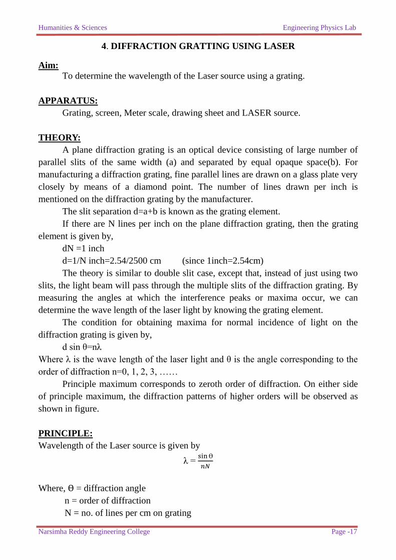
THEORY:

A plane diffraction grating is an optical device consisting of large number of

parallel slits of the same width (a) and separated by equal opaque space(b). For

manufacturing a diffraction grating, fine parallel lines are drawn on a glass plate very

closely by means of a diamond point. The number of lines drawn per inch is

mentioned on the diffraction grating by the manufacturer.

The slit separation d=a+b is known as the grating element.

If there are N lines per inch on the plane diffraction grating, then the grating

element is given by,

dN =1 inch

d=1/N inch=2.54/2500 cm (since 1inch=2.54cm)

The theory is similar to double slit case, except that, instead of just using two

slits, the light beam will pass through the multiple slits of the diffraction grating. By

measuring the angles at which the interference peaks or maxima occur, we can

determine the wave length of the laser light by knowing the grating element.

The condition for obtaining maxima for normal incidence of light on the

diffraction grating is given by,

d sin θ=nλ

Where λ is the wave length of the laser light and θ is the angle corresponding to the

order of diffraction n=0, 1, 2, 3, ……

Principle maximum corresponds to zeroth order of diffraction. On either side

of principle maximum, the diffraction patterns of higher orders will be observed as

shown in figure.

PRINCIPLE:

Wavelength of the Laser source is given by

λ =

Where, = diffraction angle

n = order of diffraction

N = no. of lines per cm on grating



EXPERIMENTAL ARRANGEMENT:

PROCEDURE:

Keep the grating in front of the laser beam such that the light is incident

normally on it. When laser light falls on the grating, the diffraction pattern is

produced on the screen in the form of bright spots which are called maxima. The

central maximum along with other maxima which are formed on either side of it

symmetrically can be seen on the screen. The positions of these bright spots can be

recorded on the graph sheet which is attached on the screen. The bright spot next to

central maxima is called the first order maxima and the light next to first order is

called second order maxima and so on. Each of the maxima corresponds to a specific

diffraction angle θ which can be measured by trigonometry. The distance central

maxima to the first order on the left are to be noted as d1 and the distance from the

central maxima to the first order on the right side is to be noted as d2. Repeat the

experiment for higher orders of diffraction and tabulate readings. Measure the

distance between the grating and the screen and tabulate it as D.

θ L

Central

Maxima

First

Order

First

Order

Second

Order

Second

Order

Screen

Single Slit

Width a =

cm

Laser

Source

Y sin θ ≈

Y/L

Diffraction

grating

Diffraction

grating



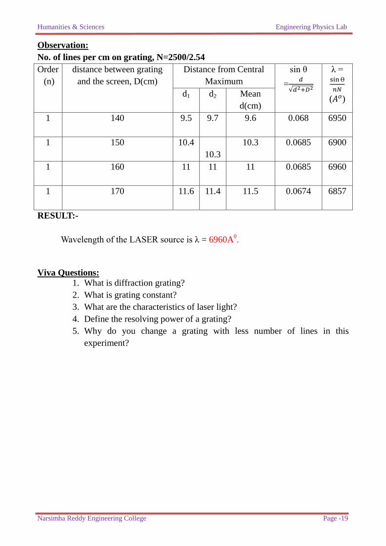
Observation:

No. of lines per cm on grating, N=2500/2.54

Order

(n)

distance between grating

and the screen, D(cm)

Distance from Central

Maximum

sin θ

=

√

λ =

( ) d1 d2 Mean

d(cm)

1 140 9.5 9.7 9.6 0.068 6950

1 150 10.4

10.3

10.3 0.0685 6900

1 160 11 11

11 0.0685 6960

1 170 11.6 11.4

11.5 0.0674 6857

RESULT:-

Wavelength of the LASER source is λ = 6960A0.

Viva Questions:

1. What is diffraction grating?

2. What is grating constant?

3. What are the characteristics of laser light?

4. Define the resolving power of a grating?

5. Why do you change a grating with less number of lines in this

experiment?



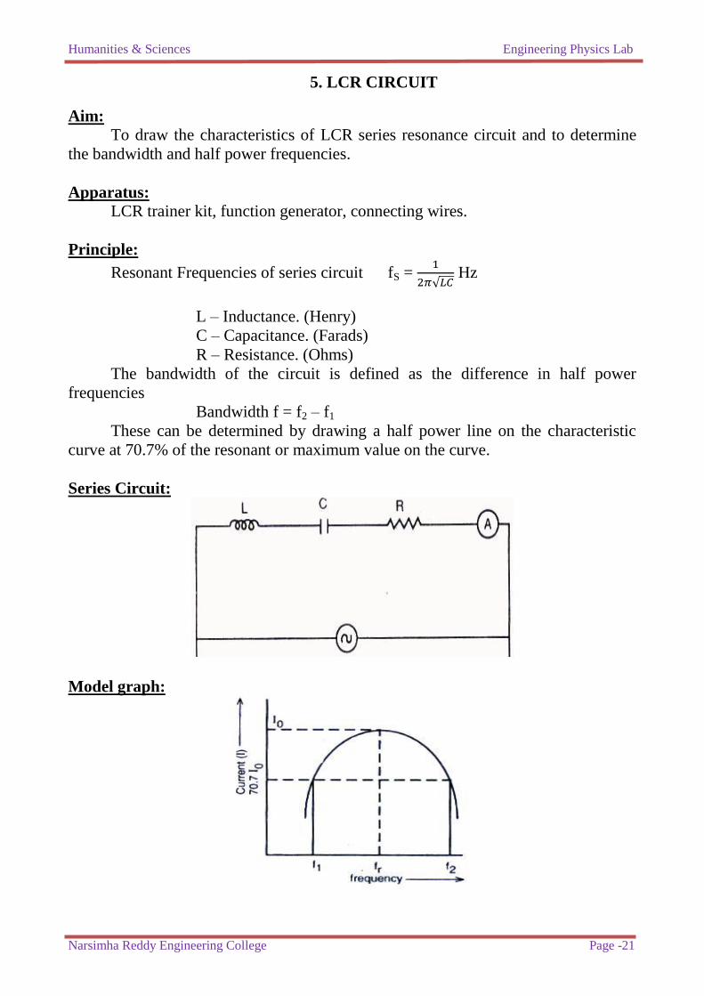
5. LCR CIRCUIT

Aim:

To draw the characteristics of LCR series resonance circuit and to determine

the bandwidth and half power frequencies.

Apparatus:

LCR trainer kit, function generator, connecting wires.

Principle:

Resonant Frequencies of series circuit fS =

√ Hz

L – Inductance. (Henry)

C – Capacitance. (Farads)

R – Resistance. (Ohms)

The bandwidth of the circuit is defined as the difference in half power

frequencies

Bandwidth f = f2 – f1

These can be determined by drawing a half power line on the characteristic

curve at 70.7% of the resonant or maximum value on the curve.

Series Circuit:

Model graph:



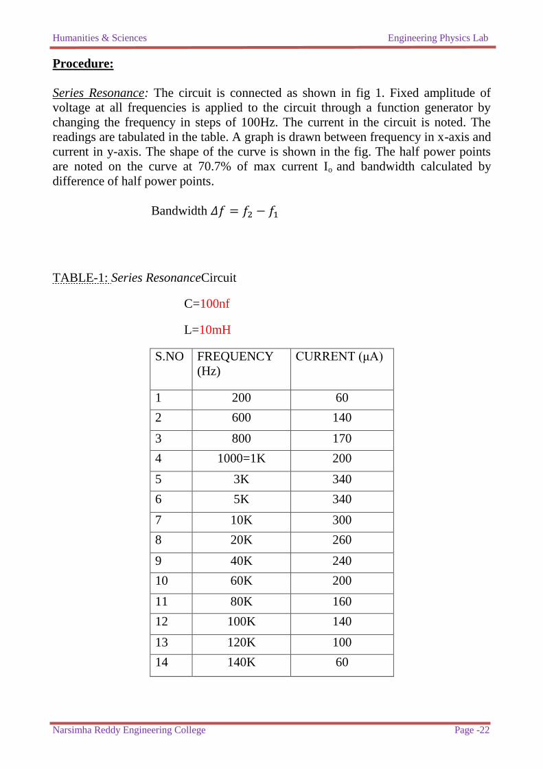
Procedure:

Series Resonance: The circuit is connected as shown in fig 1. Fixed amplitude of

voltage at all frequencies is applied to the circuit through a function generator by

changing the frequency in steps of 100Hz. The current in the circuit is noted. The

readings are tabulated in the table. A graph is drawn between frequency in x-axis and

current in y-axis. The shape of the curve is shown in the fig. The half power points

are noted on the curve at 70.7% of max current Io and bandwidth calculated by

difference of half power points.

Bandwidth

TABLE-1: Series ResonanceCircuit

C=100nf

L=10mH

S.NO FREQUENCY

(Hz)

CURRENT (μA)

1 200 60

2 600 140

3 800 170

4 1000=1K 200

5 3K 340

6 5K 340

7 10K 300

8 20K 260

9 40K 240

10 60K 200

11 80K 160

12 100K 140

13 120K 100

14 140K 60



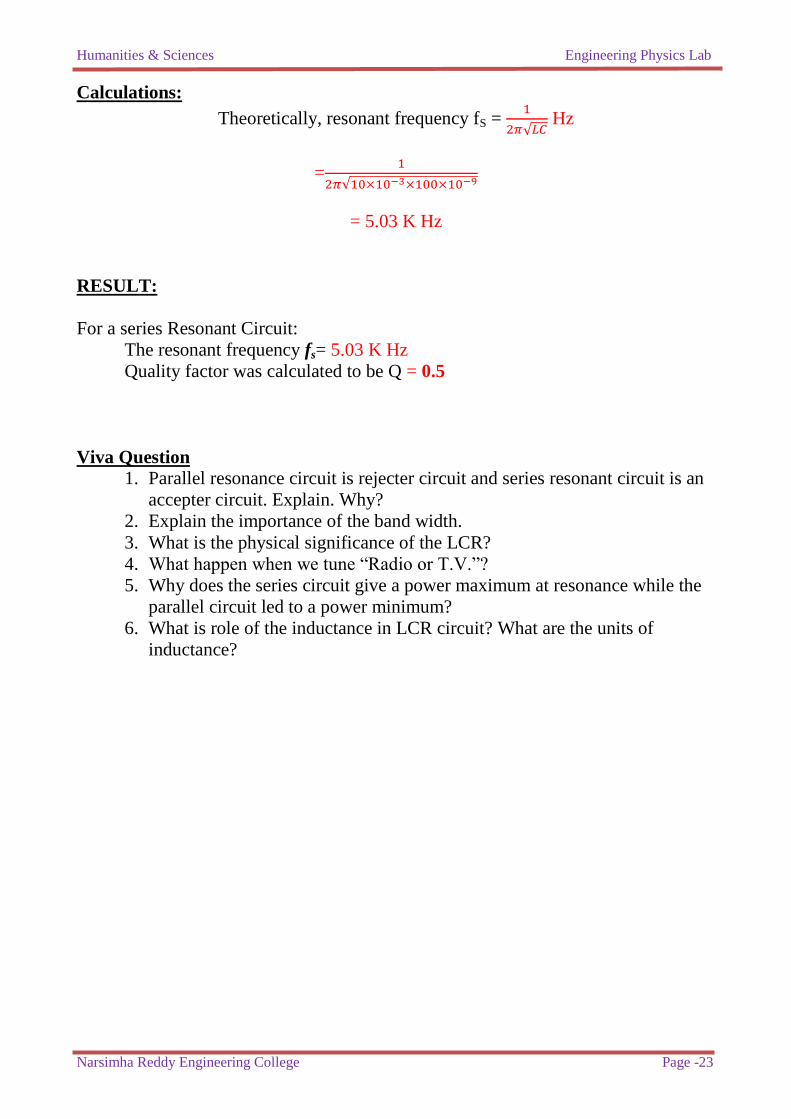
Calculations:

Theoretically, resonant frequency fS =

√ Hz

=

√

= 5.03 K Hz

RESULT:

For a series Resonant Circuit:

The resonant frequency fs= 5.03 K Hz

Quality factor was calculated to be Q = 0.5

Viva Question

1. Parallel resonance circuit is rejecter circuit and series resonant circuit is an

accepter circuit. Explain. Why?

2. Explain the importance of the band width.

3. What is the physical significance of the LCR?

4. What happen when we tune “Radio or T.V.”?

5. Why does the series circuit give a power maximum at resonance while the

parallel circuit led to a power minimum?

6. What is role of the inductance in LCR circuit? What are the units of

inductance?



6(a). Optical fiber-Numerical Aperture

Aim: To determine the Numerical aperture of the given optical fiber.

Apparatus: Optical fiber trainer module, optical fiber cables, NA jig.

Formula:

NA = sin∝ =

√

Acceptance angle = sin 𝑁

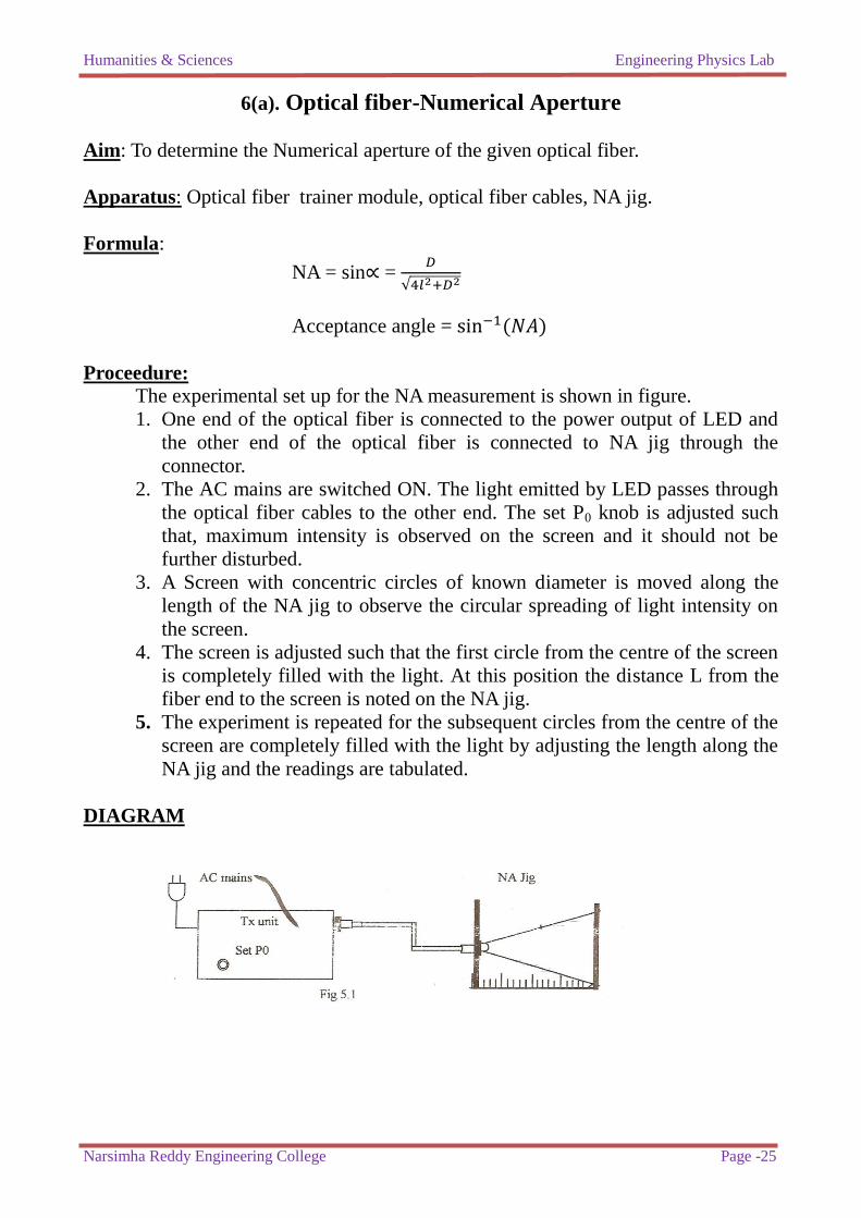
Proceedure: The experimental set up for the NA measurement is shown in figure.

1. One end of the optical fiber is connected to the power output of LED and

the other end of the optical fiber is connected to NA jig through the

connector.

2. The AC mains are switched ON. The light emitted by LED passes through

the optical fiber cables to the other end. The set P0 knob is adjusted such

that, maximum intensity is observed on the screen and it should not be

further disturbed.

3. A Screen with concentric circles of known diameter is moved along the

length of the NA jig to observe the circular spreading of light intensity on

the screen.

4. The screen is adjusted such that the first circle from the centre of the screen

is completely filled with the light. At this position the distance L from the

fiber end to the screen is noted on the NA jig.

5. The experiment is repeated for the subsequent circles from the centre of the

screen are completely filled with the light by adjusting the length along the

NA jig and the readings are tabulated.

DIAGRAM



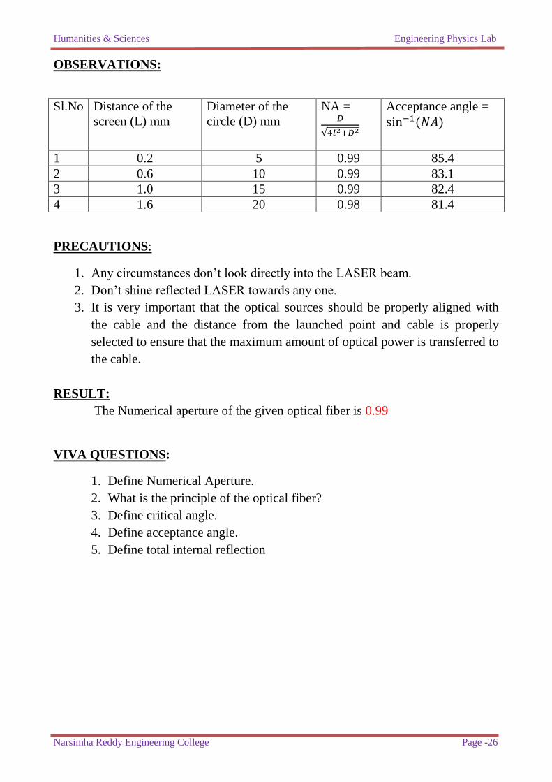
OBSERVATIONS:

Sl.No Distance of the

screen (L) mm

Diameter of the

circle (D) mm

NA =

√

Acceptance angle =

sin 𝑁

1 0.2 5 0.99 85.4

2 0.6 10 0.99 83.1

3 1.0 15 0.99 82.4

4 1.6 20 0.98 81.4

PRECAUTIONS:

1. Any circumstances don‟t look directly into the LASER beam.

2. Don‟t shine reflected LASER towards any one.

3. It is very important that the optical sources should be properly aligned with

the cable and the distance from the launched point and cable is properly

selected to ensure that the maximum amount of optical power is transferred to

the cable.

RESULT:

The Numerical aperture of the given optical fiber is 0.99

VIVA QUESTIONS:

1. Define Numerical Aperture.

2. What is the principle of the optical fiber?

3. Define critical angle.

4. Define acceptance angle.

5. Define total internal reflection



6(b). Optical fiber-Bending Losses

AIM: To determine the losses in optical fiber due to macro bending

APPARATUS: Optical fiber trainer module, optical fiber cables of different lengths,

mandrel, DMM.

FORMULAE: Loss is given by

10 log (vo/vo‟)

THEORY: Attenuation result primarily from absorption and scattering of light.

Attenuation also results from a number of effects like, fiber bending, fiber joints,

improper cleaving and also splicing due to axial displacement and mismatch of core

diameters of fibers. But here, we study the attenuation due to macro bending.

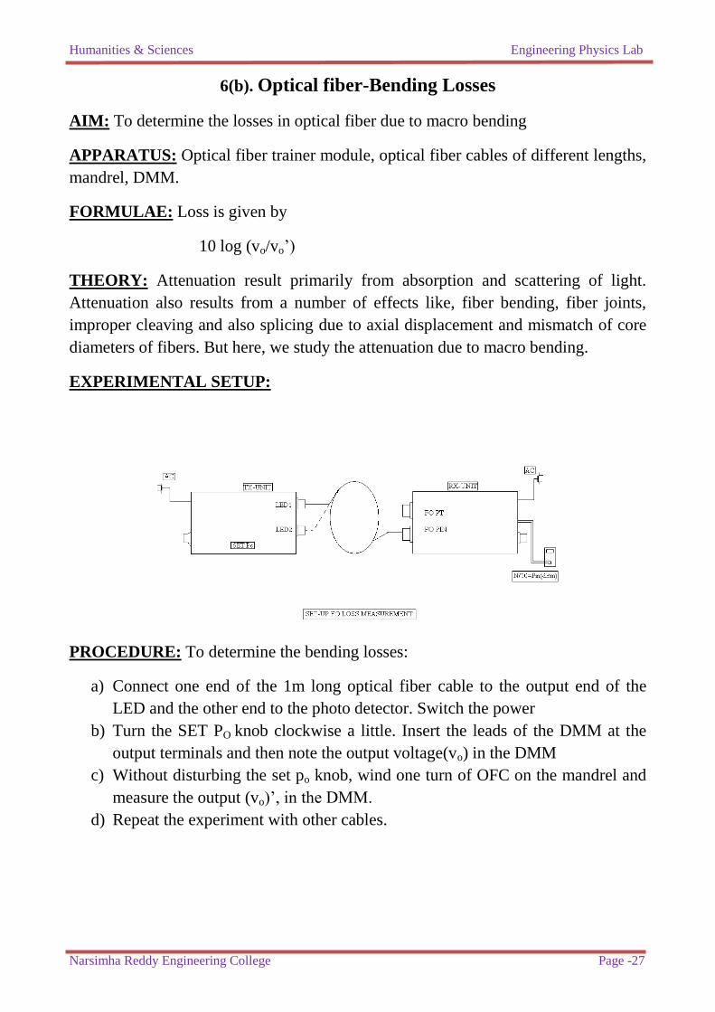
EXPERIMENTAL SETUP:

PROCEDURE: To determine the bending losses:

a) Connect one end of the 1m long optical fiber cable to the output end of the

LED and the other end to the photo detector. Switch the power

b) Turn the SET PO knob clockwise a little. Insert the leads of the DMM at the

output terminals and then note the output voltage(vo) in the DMM

c) Without disturbing the set po knob, wind one turn of OFC on the mandrel and

measure the output (vo)‟, in the DMM.

d) Repeat the experiment with other cables.



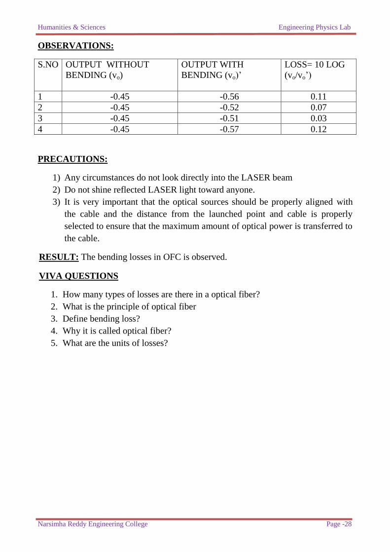
OBSERVATIONS:

S.NO OUTPUT WITHOUT

BENDING (vo)

OUTPUT WITH

BENDING (vo)‟

LOSS= 10 LOG

(vo/vo‟)

1 -0.45 -0.56 0.11

2 -0.45 -0.52 0.07

3 -0.45 -0.51 0.03

4 -0.45 -0.57 0.12

PRECAUTIONS:

1) Any circumstances do not look directly into the LASER beam

2) Do not shine reflected LASER light toward anyone.

3) It is very important that the optical sources should be properly aligned with

the cable and the distance from the launched point and cable is properly

selected to ensure that the maximum amount of optical power is transferred to

the cable.

RESULT: The bending losses in OFC is observed.

VIVA QUESTIONS

1. How many types of losses are there in a optical fiber?

2. What is the principle of optical fiber

3. Define bending loss?

4. Why it is called optical fiber?

5. What are the units of losses?



7. CHARACTERISTICS OF LED

Aim: To study the characteristics of light emitting diode.

Apparatus: LED trainer kit, connecting probes.

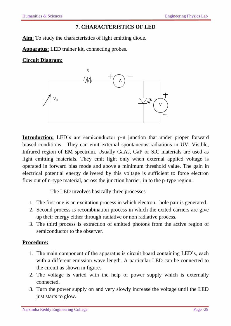
Circuit Diagram:

Introduction: LED‟s are semiconductor p-n junction that under proper forward

biased conditions. They can emit external spontaneous radiations in UV, Visible,

Infrared region of EM spectrum. Usually GaAs, GaP or SiC materials are used as

light emitting materials. They emit light only when external applied voltage is

operated in forward bias mode and above a minimum threshold value. The gain in

electrical potential energy delivered by this voltage is sufficient to force electron

flow out of n-type material, across the junction barrier, in to the p-type region.

The LED involves basically three processes

1. The first one is an excitation process in which electron –hole pair is generated.

2. Second process is recombination process in which the exited carriers are give

up their energy either through radiative or non radiative process.

3. The third process is extraction of emitted photons from the active region of

semiconductor to the observer.

Procedure:

1. The main component of the apparatus is circuit board containing LED‟s, each

with a different emission wave length. A particular LED can be connected to

the circuit as shown in figure.

2. The voltage is varied with the help of power supply which is externally

connected.

3. Turn the power supply on and very slowly increase the voltage until the LED

just starts to glow.

A

V

R

Vin



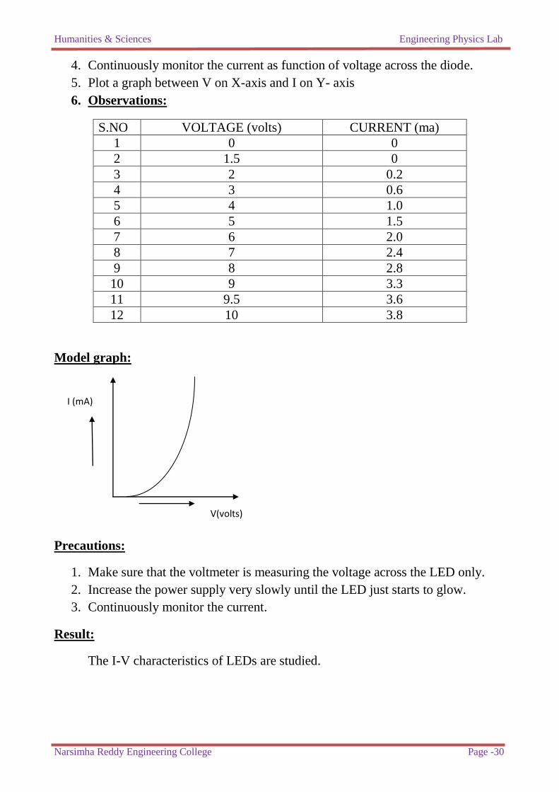
4. Continuously monitor the current as function of voltage across the diode.

5. Plot a graph between V on X-axis and I on Y- axis

6. Observations:

S.NO VOLTAGE (volts) CURRENT (ma)

1 0 0

2 1.5 0

3 2 0.2

4 3 0.6

5 4 1.0

6 5 1.5

7 6 2.0

8 7 2.4

9 8 2.8

10 9 3.3

11 9.5 3.6

12 10 3.8

Model graph:

Precautions:

1. Make sure that the voltmeter is measuring the voltage across the LED only.

2. Increase the power supply very slowly until the LED just starts to glow.

3. Continuously monitor the current.

Result:

The I-V characteristics of LEDs are studied.

I (mA)

V(volts)

V (volts)



Viva questions:

1. How does an LED emit light?

2. What is the difference between an ordinary diode and an LED?

3. Which type of materials is used to manufacture LED?

4. What are the applications of LED?



8. SOLAR CELL CHARACTERISTICS

AIM:

To determine the characteristics of solar cell.

APPARATUS:

Solar cell trainer kit, Solar cell, Variable light source.

FORMULAE:

Fill factor, f=

Where, ImXVm----- maximum obtainable power

Isc- Short circuit current

Voc- Open Circuit Voltage

THEORY:

If the depletion of unbiased junction is illuminated, charge separation takes

place, resulting in forward bias on the junction. Such device having large area

junction very close to the surface is capable of delivering power and is known as

SOLAR CELL. The cell converts directly solar energy into electricity.

The Solar Cell radiation is proportional to the delivered power of cell. The

efficiency of a cell is expressed in terms of the electrical power output compared

with the power in the incident Photon Flux. The efficiency of Solar Cell depends on

the fraction of light reflected from the surface and the fraction absorbed before

reaching the junction. Silicon is widely used for Solar Cells.

CIRCUIT DIAGRAM:



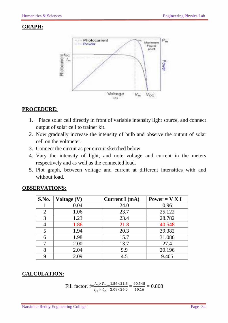
GRAPH:

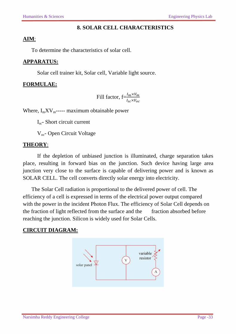
PROCEDURE:

1. Place solar cell directly in front of variable intensity light source, and connect

output of solar cell to trainer kit.

2. Now gradually increase the intensity of bulb and observe the output of solar

cell on the voltmeter.

3. Connect the circuit as per circuit sketched below.

4. Vary the intensity of light, and note voltage and current in the meters

respectively and as well as the connected load.

5. Plot graph, between voltage and current at different intensities with and

without load.

OBSERVATIONS:

S.No. Voltage (V) Current I (mA) Power = V X I

1 0.04 24.0 0.96

2 1.06 23.7 25.122

3 1.23 23.4 28.782

4 1.86 21.8 40.548

5 1.94 20.3 39.382

6 1.98 15.7 31.086

7 2.00 13.7 27.4

8 2.04 9.9 20.196

9 2.09 4.5 9.405

CALCULATION:

Fill factor, f=

=

=

= 0.808



RESULT: Characteristics of solar cell are studied.

Viva Question:

1. What factors may contribute to the lack of efficiency of the solar cell?

2. What does the energy output of a solar cell depend up on?

3. Why is it important to find out the highest power output for a solar cell?

4. Depending up on your observations , what are the best conditions for gaining

the maximum power from a solar cell?



9. ENERGY BAND GAP

Aim:

To determine the width of the forbidden energy gap in a semiconductor

material using reverse biased p-n junction diode method.

Apparatus:

Power supply, heating arrangement, thermometer, micro ammeter, germanium

diode.

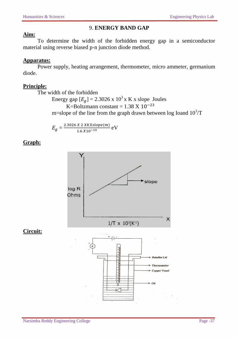
Principle:

The width of the forbidden

Energy gap [ ] = 2.3026 x 103 x K x slope Joules

K=Boltzmann constant = 1.38 X

m=slope of the line from the graph drawn between log Ioand 103/T

=

eV

Graph:

Circuit:



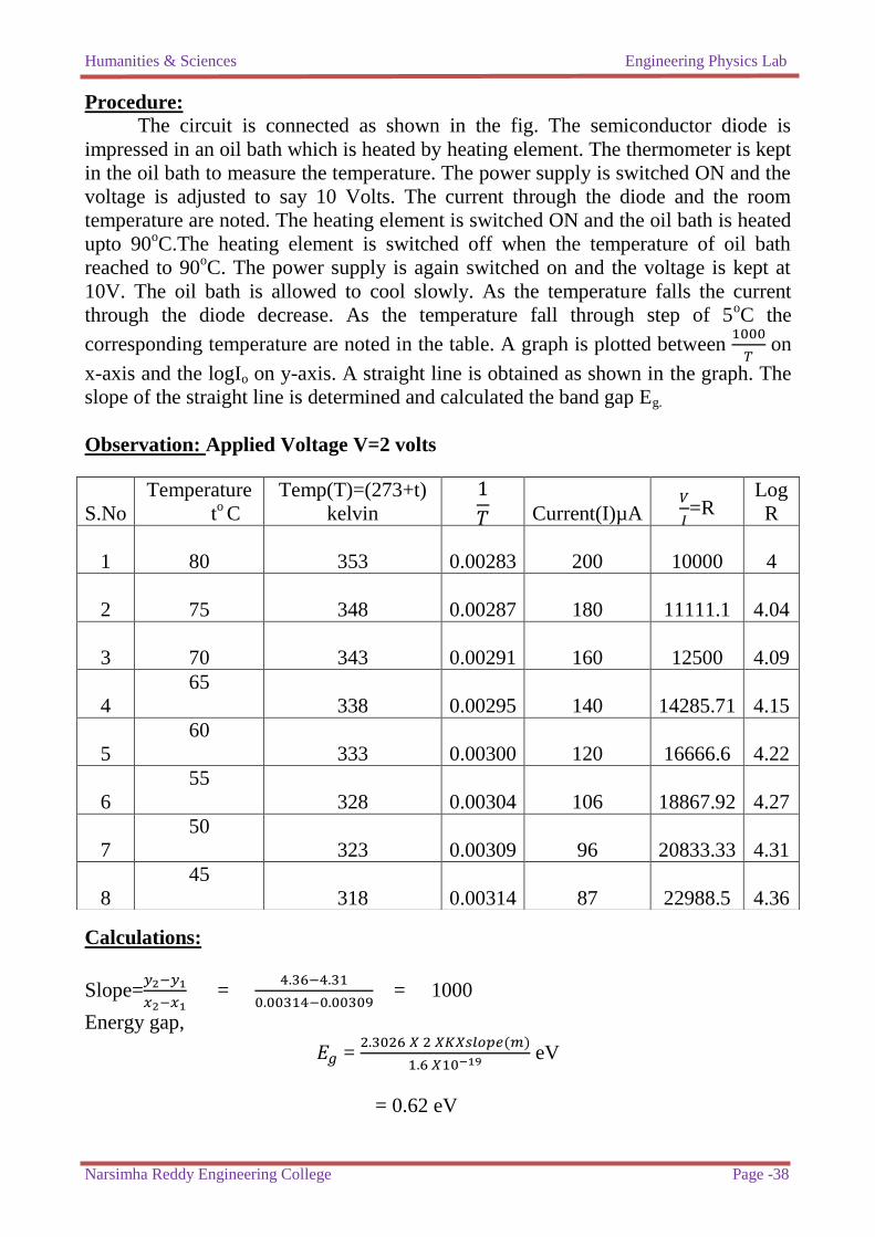
Procedure: The circuit is connected as shown in the fig. The semiconductor diode is

impressed in an oil bath which is heated by heating element. The thermometer is kept

in the oil bath to measure the temperature. The power supply is switched ON and the

voltage is adjusted to say 10 Volts. The current through the diode and the room

temperature are noted. The heating element is switched ON and the oil bath is heated

upto 90oC.The heating element is switched off when the temperature of oil bath

reached to 90oC. The power supply is again switched on and the voltage is kept at

10V. The oil bath is allowed to cool slowly. As the temperature falls the current

through the diode decrease. As the temperature fall through step of 5oC the

corresponding temperature are noted in the table. A graph is plotted between

on

x-axis and the logIo on y-axis. A straight line is obtained as shown in the graph. The

slope of the straight line is determined and calculated the band gap Eg.

Observation: Applied Voltage V=2 volts

Calculations:

Slope=

=

= 1000

Energy gap,

=

eV

= 0.62 eV

S.No

Temperature

to C

Temp(T)=(273+t)

kelvin

Current(I)µA

=R

Log

R

1 80 353 0.00283 200 10000 4

2

75 348 0.00287 180 11111.1 4.04

3

70 343 0.00291 160 12500 4.09

4

65

338 0.00295 140 14285.71 4.15

5

60

333 0.00300 120 16666.6 4.22

6

55

328 0.00304 106 18867.92 4.27

7

50

323 0.00309 96 20833.33 4.31

8

45

318 0.00314 87 22988.5 4.36



Precautions:

1. The current flow should not be too high, if the current is high then the internal

heating of the device will occur. This will cause actual temperature of the

junction to be higher than the measured value. This will produce non-linearity

in the curve.

2. There may be contact potentials, thermo emfs and meter dc offsets which must

be add and subtract from the readings.

3. Poor contacts result in huge variations in the results and must be carefully

soldered.

4. It is better to repeat a few measurements at end of each run to check the source

of error.

RESULT:

Energy Gap of p-n junction diode = 0.62 eV

Viva Questions:

1. What is a semiconductor?

2. Why Germanium specimen is preferred over silicon specimen? Why?

3. What are the units of energy gap?

4. Differentiate between conductors, semiconductors and insulators.

5. What is meant by doping?

6. What happens if the temperature of oil bath exceeds 90o C?



10. STEWART & GEE’S EXPERIMENT

(Magnetic field along the axis of a coil)

AIM:

To determine the field of induction at several points on the axis of a circular

coil carrying current using Stewart and Gee‟s method.

Apparatus:

Stewart gee‟s experiment, battery eliminator, ammeter, connecting wires,

commutator, rheostat, plug key, compass.

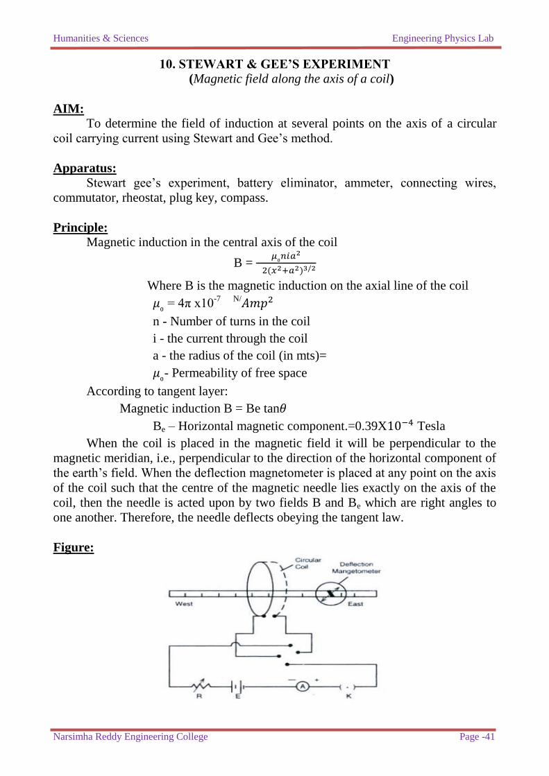
Principle: Magnetic induction in the central axis of the coil

B =

Where B is the magnetic induction on the axial line of the coil

= 4π x10-7 N/

n - Number of turns in the coil

i - the current through the coil

a - the radius of the coil (in mts)=

- Permeability of free space

According to tangent layer:

Magnetic induction B = Be tan

Be – Horizontal magnetic component.=0.39X Tesla

When the coil is placed in the magnetic field it will be perpendicular to the

magnetic meridian, i.e., perpendicular to the direction of the horizontal component of

the earth‟s field. When the deflection magnetometer is placed at any point on the axis

of the coil such that the centre of the magnetic needle lies exactly on the axis of the

coil, then the needle is acted upon by two fields B and Be which are right angles to

one another. Therefore, the needle deflects obeying the tangent law.

Figure:



Procedure:

With the help of the deflection magnetometer and a chalk, a long line of about

one meter is drawn on the working table to represent the magnetic meridian. Draw

the perpendicular lines to this line and place the coil of Stewart and gee‟s apparatus

in the magnetic meridian line. This coil is connected by connecting wires as shown

the fig. The deflection magnetometer is set at the centre of the coil and rotated to

make the aluminum pointer reading (0, 0) in the magnetometer.

The deflection reading before and after reversal of the current with the help of

commutator in the circuit are noted at distance d=0. The magnetometer is moved

towards east along the axis of the coil in steps of 5cm at a time. At each position the

deflections before and after reversal of current are noted. The deflections are noted

upto 20cm on the x-axis east side. The mean deflection is noted as .

The experiment is repeated by shifting the magnetometer towards west side

from the centre of the coil in steps of 5cm each time and deflections are noted before

and after reversal of current. The mean deflection is denoted as . A graph is drawn

between the distance on x-axis and the θ on y-axis. The slope of the curve is shown

in the fig. The points A and B marked on the curve lie at distance equal to half the

radius of the coil on either side of the coil.

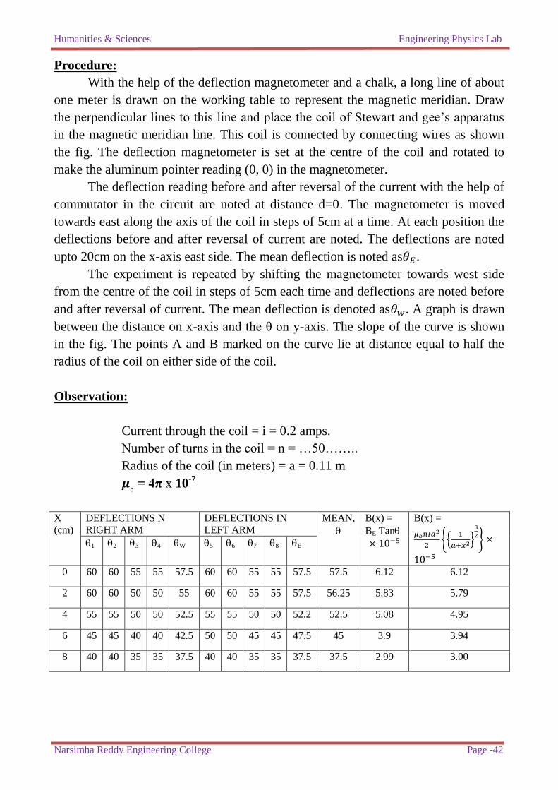
Observation:

Current through the coil = i = 0.2 amps.

Number of turns in the coil = n = …50……..

Radius of the coil (in meters) = a = 0.11 m

= 4π x 10-7

X

(cm)

DEFLECTIONS N

RIGHT ARM

DEFLECTIONS IN

LEFT ARM

MEAN,

B(x) =

BE Tan

B(x) =

{{

}

}

1 2 3 4 W 5 6 7 8 E

0 60 60 55 55 57.5 60 60 55 55 57.5 57.5 6.12 6.12

2 60 60 50 50 55 60 60 55 55 57.5 56.25 5.83 5.79

4 55 55 50 50 52.5 55 55 50 50 52.2 52.5 5.08 4.95

6 45 45 40 40 42.5 50 50 45 45 47.5 45 3.9 3.94

8 40 40 35 35 37.5 40 40 35 35 37.5 37.5 2.99 3.00



Precautions:

The ammeter, voltmeter should keep away from the deflection magnetometer

because these meters will affect the deflection in magnetometer.

The current passing through rheostat will produce magnetic field and magnetic

field produced by the permanent magnet inside the ammeter will affect the

deflection reading.

Result:

It will be found that for each distance(X) the values in the last two columns are

found to be equal in table.

Viva Questions:

1. What is the direction of magnetic field at the centre of the coil?

2. Define magnetic meridian?

3. Where magnetic field is maximum in Stewart-Gee‟s method?

4. Define magnetic field induction (B), give its units?

5. State some of the applications of magnetic field produced by a circular coil?

6. Among Helmholtz galvanometer and moving coil galvanometer, which one is

more sensitive, explain?

7. in the preset experiment why galvanometer should be kept away from

ammeter and rheostat?



11. Dispersive Power of the Prism

Aim:

To determine the dispersive power of the material of the given prism.

Apparatus:

Spectrometer, Mercury vapor lamp, glass prism, reading lens.

Principle:

The dispersive power of a prism = ω =

- Refractive index of Red light.

- Refractive index of blue light.

μ =

Refractive index μ =

A - Angle of the prism.

D - Minimum deviation.

Adjustments of the Spectrometer: The essential parts of the spectrometer are a)the

telescope b)collimator c)Prism table

Telescope adjustment:

The telescope is turned towards a distant object and its length is adjusted until

the distant object is clearly seen in the plane of the cross-wires.



The telescope is turned towards a white wall and the eyepiece is adjusted so

that the cross-wire is very clearly seen. This ensures that whenever an image is

clearly seen on the cross-wire, it may be taken that the rays entering the telescope

constitute a parallel bundle.

Collimeter adjustment:

The slit of the collimeter is illuminated with light. The telescope is turned to

view the image of the slit and the collimeter screw is adjusted such that a clear image

of the slit is obtained without parallel in the plane of the cross-wire. This slit is

narrowed by adjustment of the slit screw and coincides with vertical cross-wire of the

telescope.

Prism table and base of the instrument:

The instrument base is leveled by adjusting the leveling screws with the help

of spirit level. And prism table also leveled by adjusting the leveling screws with the

help of the spirit level.

Scale Adjustment:

The scale adjustment zero of the Vernier scale should coincide with zero of the

main scale by Vernier adjustment when the cross-wire is coincided with slit image.

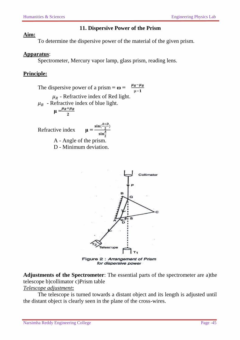
Procedure:

The prism is placed on the prism table with the ground surface of the prism to

the left or right side of the collimeter. The ray of light passing through the Collimeter

strikes the polished surface BC of the prism from the face AC. The deviated ray is

seen as spectrum through the telescope in position T2.

Looking at the spectrum the prism table is now slowly moved on to one side,

so that the spectrum moves towards the undeviated path of the beam. At one position

the spectrum starts turning back even though the prism table is moved in the same

direction. This position is called as minimum deviation position. At this position stop

the prism and cross-wire is made to coincide with red color and note the reading with

the help of the Vernier scale, recorded in the observation table. This procedure is

repeated with blue color and refractive index of these colors is calculated. This

dispersive power of the prism is calculated using given above formula.

Observations:

Least count of the Vernier of the spectrometer = 1‟

Angle of the prism (A) –60o

Direct ray reading

Vernier 1 –180o

Vernier 2 –360o



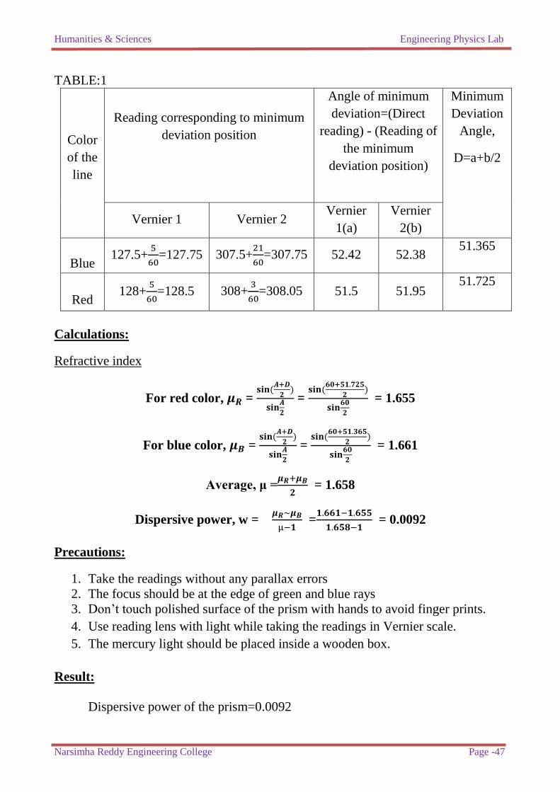
TABLE:1

Color

of the

line

Reading corresponding to minimum

deviation position

Angle of minimum

deviation=(Direct

reading) - (Reading of

the minimum

deviation position)

Minimum

Deviation

Angle,

D=a+b/2

Vernier 1 Vernier 2 Vernier

1(a)

Vernier

2(b)

Blue 127.5+

=127.75 307.5+

=307.75 52.42 52.38

51.365

Red 128+

=128.5 308+

=308.05 51.5 51.95

51.725

Calculations:

Refractive index

For red color, =

=

= 1.655

For blue color, =

=

= 1.661

Average, μ =

= 1.658

Dispersive power, w =

=

= 0.0092

Precautions:

1. Take the readings without any parallax errors

2. The focus should be at the edge of green and blue rays

3. Don‟t touch polished surface of the prism with hands to avoid finger prints.

4. Use reading lens with light while taking the readings in Vernier scale.

5. The mercury light should be placed inside a wooden box.

Result:

Dispersive power of the prism=0.0092



Viva Questions:

1. What happen when rays of light of different colors travel in a glass prism

2. What is minimum deviation

3. What are the advantages in putting the prism in the minimum deviation

position

4. What are the spectrometer adjustment

5. Explain the Collimeter adjustment

6. What is telescope adjustment

7. What are the light properties

8. What is the visible wave length range

9. How to place the prism on the table

10. What is A0 unit?

Applications:

1. The dispersion of light in optical fibers.

2. The brilliance of diamond is due to its large dispersion.



12. NEWTON’S RINGS

Aim:

To determine the Radius of curvature of the Plano convex lens (R) by forming

Newton‟s rings.

Apparatus:

Travelling microscope, sodium vapour lamp, Plano convex lens, a thick glass

plate, a magnifying glass.

Principle:

λ =

R =

λ - Wave length of sodium light source.

R - Radius of curvature of the of Plano convex lens.

Dm- Diameter of the mth

ring.

Dn - Diameter of the nth

ring.

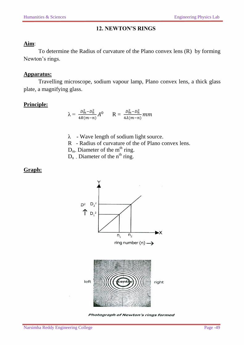
Graph:



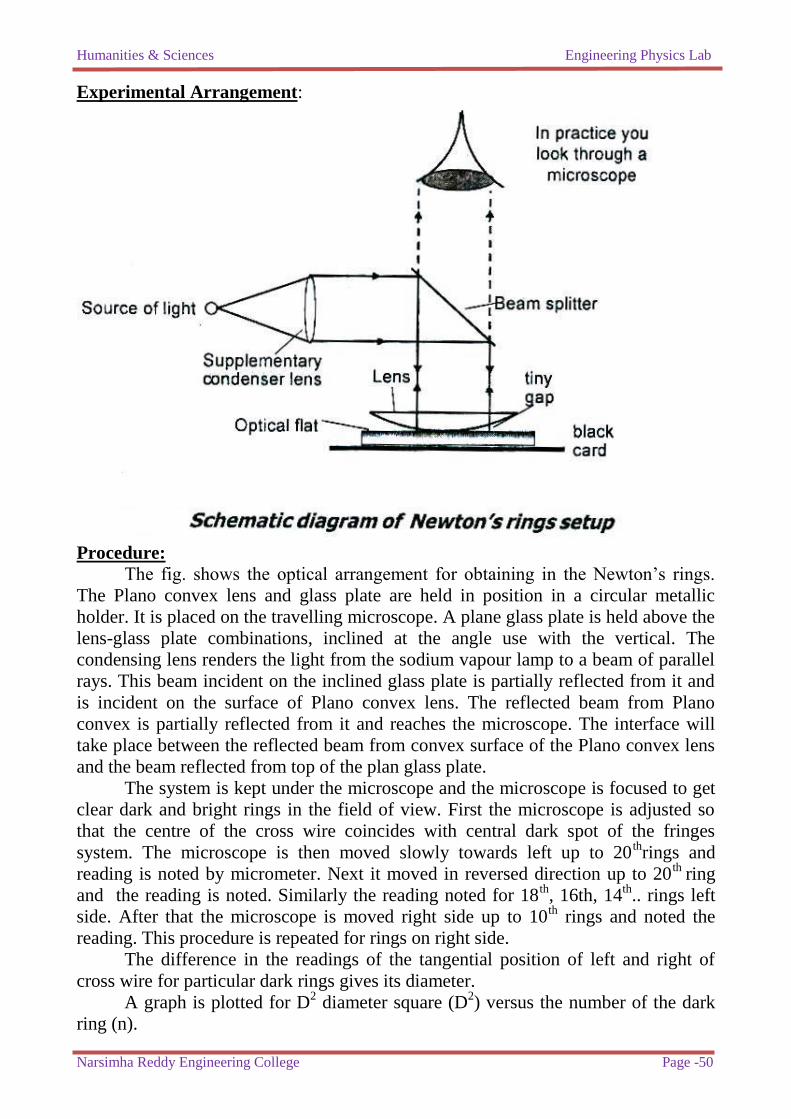
Experimental Arrangement:

Procedure:

The fig. shows the optical arrangement for obtaining in the Newton‟s rings.

The Plano convex lens and glass plate are held in position in a circular metallic

holder. It is placed on the travelling microscope. A plane glass plate is held above the

lens-glass plate combinations, inclined at the angle use with the vertical. The

condensing lens renders the light from the sodium vapour lamp to a beam of parallel

rays. This beam incident on the inclined glass plate is partially reflected from it and

is incident on the surface of Plano convex lens. The reflected beam from Plano

convex is partially reflected from it and reaches the microscope. The interface will

take place between the reflected beam from convex surface of the Plano convex lens

and the beam reflected from top of the plan glass plate.

The system is kept under the microscope and the microscope is focused to get

clear dark and bright rings in the field of view. First the microscope is adjusted so

that the centre of the cross wire coincides with central dark spot of the fringes

system. The microscope is then moved slowly towards left up to 20thrings and

reading is noted by micrometer. Next it moved in reversed direction up to 20th

ring

and the reading is noted. Similarly the reading noted for 18th

, 16th, 14th

.. rings left

side. After that the microscope is moved right side up to 10th

rings and noted the

reading. This procedure is repeated for rings on right side.

The difference in the readings of the tangential position of left and right of

cross wire for particular dark rings gives its diameter.

A graph is plotted for D2 diameter square (D

2) versus the number of the dark

ring (n).



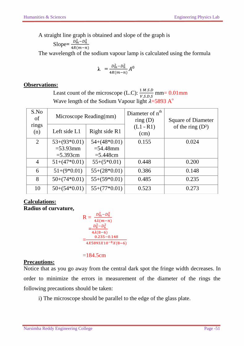
A straight line graph is obtained and slope of the graph is

Slope=

The wavelength of the sodium vapour lamp is calculated using the formula

λ =

Observations:

Least count of the microscope (L.C):

mm= 0.01mm

Wave length of the Sodium Vapour light 𝜆=5893 Ao

Calculations:

Radius of curvature,

R =

=

=

=184.5cm

Precautions:

Notice that as you go away from the central dark spot the fringe width decreases. In

order to minimize the errors in measurement of the diameter of the rings the

following precautions should be taken:

i) The microscope should be parallel to the edge of the glass plate.

S.No

of

rings

(n)

Microscope Reading(mm) Diameter of n

th

ring (D)

(L1 R1)

(cm)

Square of Diameter

of the ring (D²) Left side L1 Right side R1

2 53+(93*0.01)

=53.93mm

=5.393cm

54+(48*0.01)

=54.48mm

=5.448cm

0.155 0.024

4 51+(47*0.01) 55+(5*0.01) 0.448 0.200

6 51+(9*0.01) 55+(28*0.01) 0.386 0.148

8 50+(74*0.01) 55+(59*0.01) 0.485 0.235

10 50+(54*0.01) 55+(77*0.01) 0.523 0.273



ii) If you place the cross wire tangential to the outer side of a perpendicular

ring on one side of the central spot then the cross wire should be placed

tangential to the inner side of the same ring on the other side of the central

spot.

iii) The traveling microscope should move only in one direction

RESULT:

Radius of curvature of the given plano convex lens R =184.5cm

Viva Questions:


2. How are the Newton‟s rings formed?

3. Where are the rings formed?

4. Why are the rings circular and concentric?

5. Why is the central spot dark?

6. Why should lens of larger R be used in the experiment?

7. How will the rings change if we introduce a little water between the lens and

the plate?

8. What will happen if white light is used in place of sodium light?

9. What are the engineering applications of Newton‟s rings?



13. DIFFRACTION GRATING

AIM: To determine the wave length of a given light using diffraction grating with

normal incidence method.

Apparatus:

Plane diffraction grating, spectrometer, sodium vapour lamp, reading lens.

Principle:

λ=

=

λ - Wavelength of light.

d – Grating spacing d =

N is no. of lines per cm.

n – Order of spectrum.

– Angle of deviation corresponding to nth order.

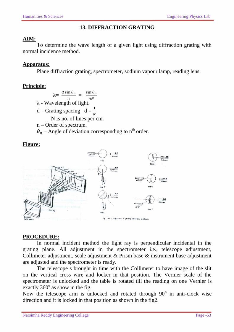
Figure:

PROCEDURE: In normal incident method the light ray is perpendicular incidental in the

grating plane. All adjustment in the spectrometer i.e., telescope adjustment,

Collimeter adjustment, scale adjustment & Prism base & instrument base adjustment

are adjusted and the spectrometer is ready.

The telescope s brought in time with the Collimeter to have image of the slit

on the vertical cross wire and locker in that position. The Vernier scale of the

spectrometer is unlocked and the table is rotated till the reading on one Vernier is

exactly 360o as show in the fig.

Now the telescope arm is unlocked and rotated through 90o in anti-clock wise

direction and it is locked in that position as shown in the fig2.



The grating is placed on the prism table with its ruled surface towards the

telescope. The grating stand should at the centre of the prism table. Then the prism

table is rotated slowly, so that a reflected image is seen in the field view of the

telescope and coincided with vertical cross wire the prism table is locked in that

position. The angle of incidence of light on grating surface is 45o as shown in

fig3.The Vernier scale is rotated along with prism table through an angle 45o so that

the grating plane becomes normal to the direction of the light as shown in fig4.

Now the telescope is unlocked and rotated to bring it in line with the

Collimeter to receive the image of the slit on the cross-wires. The telescope is slowly

rotated to the right till the image of the slit corresponding to the first order is

coinciding with cross wire and the reading is noted. The difference between the two

positions gives the angle of deviation belonging to the first order. The telescope is

rotated further right side to get the image along to second order and the angle of

deviation is calculated and the readings are noted down in the table. The wavelength

is calculated using the formula.

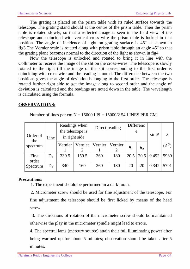
OBSERVATIONS:

Number of lines per cm N = 15000 LPI = 15000/2.54 LINES PER CM

Order of

the

spectrum

Line

Readings when

the telescope is

in right side

Direct reading

Differenc

e

sin

𝜆

Vernier

1

Vernier

2

Vernier

1

Vernier

2

( )

First

order

Spectrum

D1

D2

339.5

159.5

360

180

20.5

20.5

0.492

5930

D2

340 160 360 180 20 20 0.342 5791

Precautions:

1. The experiment should be performed in a dark room.

2. Micrometer screw should be used for fine adjustment of the telescope. For

fine adjustment the telescope should be first licked by means of the head

screw.

3. The directions of rotation of the micrometer screw should be maintained

otherwise the play in the micrometer spindle might lead to errors.

4. The spectral lams (mercury source) attain their full illuminating power after

being warmed up for about 5 minutes; observation should be taken after 5

minutes.



5. One of the essential precautions for the success of this experiment is to set

the grating normal to the incident rays (see below). Small variation on the

angle of incident causes correspondingly large error in the angle of diffraction.

If the exact normally is not observed, one find that the angle of diffraction

measured on the left and on the right are not exactly equal. Read both the

verniers to eliminate any errors due to non coincidence of the center of the

circular sale with the axis of rotation of the telescope or table.

RESULT:

Wavelength of the = 5930 .

Wavelength of the =5791 .

Viva Questions:


2. What is a diffraction grating?

3. What is meant by diffraction of light?

4. Where is the zero order fringes formed?

5. What is meant by diffraction of light?

6. What are the different types of grating?

7. Explain the normal incident method?

8. N representing _____________ per cm

vision - nrcmec.org master.pdf · vision: to emerge as a destination for higher education by...

Documents