visual explain tutorial - san diego supercomputer centerusers.sdsc.edu/~jrowley/db2/visual explain...
TRANSCRIPT

IBM®
DB2 Universal Database™
Visual Explain Tutorial
Version 8
���


IBM®
DB2 Universal Database™
Visual Explain Tutorial
Version 8
���

Before using this information and the product it supports, be sure to read the general information under Notices.
This document contains proprietary information of IBM. It is provided under a license agreement and is protected bycopyright law. The information contained in this publication does not include any product warranties, and anystatements provided in this manual should not be interpreted as such.
You can order IBM publications online or through your local IBM representative.v To order publications online, go to the IBM Publications Center at www.ibm.com/shop/publications/order
v To find your local IBM representative, go to the IBM Directory of Worldwide Contacts atwww.ibm.com/planetwide
To order DB2 publications from DB2 Marketing and Sales in the United States or Canada, call 1-800-IBM-4YOU(426-4968).
When you send information to IBM, you grant IBM a nonexclusive right to use or distribute the information in anyway it believes appropriate without incurring any obligation to you.
© Copyright International Business Machines Corporation 2000 - 2002. All rights reserved.US Government Users Restricted Rights – Use, duplication or disclosure restricted by GSA ADP Schedule Contractwith IBM Corp.

Contents
About this tutorial . . . . . . . . . . vEnvironment-specific information . . . . . vi
Lesson 1. Creating explain snapshots . . . 1Creating the explain tables . . . . . . . 1Using explain snapshots . . . . . . . . 2
Creating explain snapshots for dynamicSQL statements . . . . . . . . . . 3Creating explain snapshots for static SQLstatements . . . . . . . . . . . . 4
What’s Next . . . . . . . . . . . . 4
Lesson 2. Displaying and using an accessplan graph . . . . . . . . . . . . 5Displaying an access plan graph by choosingfrom a list of previously explained SQLstatements . . . . . . . . . . . . . 5
Reading the symbols in an access plangraph . . . . . . . . . . . . . 5Using the zoom slider to magnify parts of agraph . . . . . . . . . . . . . 6
Getting more details about the objects in agraph . . . . . . . . . . . . . . 7
Getting statistics for tables, indexes, andtable functions . . . . . . . . . . 7Getting details about operators in a graph . 8Getting statistics for functions . . . . . 8Getting statistics for tables spaces . . . . 8Getting statistics for columns in an SQLstatement . . . . . . . . . . . . 8Getting information about configurationparameters and bind options . . . . . . 9
Changing the appearance of a graph . . . . 9What’s Next . . . . . . . . . . . . 9
Lesson 3. Improving an access plan in asingle-partition database environment . . 11Working with access plan graphs . . . . . 11
Running a query with no indexes and nostatistics . . . . . . . . . . . . 12Collecting current statistics for the tablesand indexes using runstats . . . . . . 15Creating indexes on columns used to jointables in a query . . . . . . . . . 19
Creating additional indexes on tablecolumns . . . . . . . . . . . . 25
What’s Next . . . . . . . . . . . . 27
Lesson 4. Improving an access plan in apartitioned database environment . . . . 29Working with access plan graphs . . . . . 29
Running a query with no indexes and nostatistics . . . . . . . . . . . . 30Collecting current statistics for the tablesand indexes using runstats . . . . . . 33Creating indexes on columns used to jointables in a query . . . . . . . . . 37Creating additional indexes on tablecolumns . . . . . . . . . . . . 41
What’s Next . . . . . . . . . . . . 45
Appendix A. Visual Explain concepts . . . 47Access plan . . . . . . . . . . . . 47Access plan graph . . . . . . . . . . 47Access plan graph node . . . . . . . . 48Clustering. . . . . . . . . . . . . 49Container . . . . . . . . . . . . . 49Cost. . . . . . . . . . . . . . . 49Cursor blocking . . . . . . . . . . . 50Database-managed space (DMS) table space 50Dynamic SQL . . . . . . . . . . . 50Explain snapshot . . . . . . . . . . 51Explainable statement . . . . . . . . . 51Explained statement . . . . . . . . . 52Operand . . . . . . . . . . . . . 52Operator . . . . . . . . . . . . . 52CMPEXP . . . . . . . . . . . . . 53DELETE . . . . . . . . . . . . . 54EISCAN . . . . . . . . . . . . . 54FETCH. . . . . . . . . . . . . . 54FILTER. . . . . . . . . . . . . . 55GENROW. . . . . . . . . . . . . 55GRPBY. . . . . . . . . . . . . . 55HSJOIN . . . . . . . . . . . . . 56INSERT . . . . . . . . . . . . . 57IXAND . . . . . . . . . . . . . 57IXSCAN . . . . . . . . . . . . . 57MSJOIN . . . . . . . . . . . . . 58NLJOIN . . . . . . . . . . . . . 59
© Copyright IBM Corp. 2000 - 2002 iii
PIPE . . . . . . . . . . . . . . 60RETURN . . . . . . . . . . . . . 60RIDSCN . . . . . . . . . . . . . 60RQUERY . . . . . . . . . . . . . 60SORT . . . . . . . . . . . . . . 61TBSCAN . . . . . . . . . . . . . 62TEMP . . . . . . . . . . . . . . 62TQUEUE . . . . . . . . . . . . . 63UNION . . . . . . . . . . . . . 63UNIQUE . . . . . . . . . . . . . 63UPDATE . . . . . . . . . . . . . 64Optimizer . . . . . . . . . . . . . 64Package . . . . . . . . . . . . . 64Predicate . . . . . . . . . . . . . 64Query optimization class . . . . . . . . 65Selectivity of predicates . . . . . . . . 66Star joins . . . . . . . . . . . . . 67Static SQL. . . . . . . . . . . . . 68System-managed space (SMS) table spaces . . 68Table space . . . . . . . . . . . . 68Visual Explain . . . . . . . . . . . 69
Appendix B. Alphabetical list of VisualExplain operators. . . . . . . . . . 71CMPEXP . . . . . . . . . . . . . 71DELETE . . . . . . . . . . . . . 71EISCAN . . . . . . . . . . . . . 71FETCH. . . . . . . . . . . . . . 72FILTER. . . . . . . . . . . . . . 72GENROW. . . . . . . . . . . . . 72GRPBY. . . . . . . . . . . . . . 73
HSJOIN . . . . . . . . . . . . . 73INSERT . . . . . . . . . . . . . 74IXAND . . . . . . . . . . . . . 74IXSCAN . . . . . . . . . . . . . 75MSJOIN . . . . . . . . . . . . . 75NLJOIN . . . . . . . . . . . . . 76PIPE . . . . . . . . . . . . . . 77RETURN . . . . . . . . . . . . . 77RIDSCN . . . . . . . . . . . . . 77RQUERY . . . . . . . . . . . . . 78SORT . . . . . . . . . . . . . . 78TBSCAN . . . . . . . . . . . . . 79TEMP . . . . . . . . . . . . . . 80TQUEUE . . . . . . . . . . . . . 80UNION . . . . . . . . . . . . . 81UNIQUE . . . . . . . . . . . . . 81UPDATE . . . . . . . . . . . . . 81
Appendix C. DB2 concepts . . . . . . 83Databases . . . . . . . . . . . . . 83Schemas . . . . . . . . . . . . . 83Tables . . . . . . . . . . . . . . 84
Appendix D. Notices. . . . . . . . . 85Trademarks . . . . . . . . . . . . 88
Index . . . . . . . . . . . . . . 91
Contacting IBM . . . . . . . . . . 93Product information . . . . . . . . . 93
iv VE Tutorial
About this tutorial
This tutorial provides a guide to the features of DB2 Visual Explain. Bycompleting the lessons in this tutorial you will learn how Visual Explain letsyou view the access plan for explained SQL statements as a graph. You willalso learn to use the information available from such a graph to tune yourSQL queries for better performance.
Using its optimizer, DB2 examines your SQL queries and determines how bestto access your data. This path to the data is called the access plan. DB2enables you to see what the optimizer has done by allowing you to look atthe access plan that it selected to perform a particular SQL query. You can useVisual Explain to display the access plan as a graph. The graph is a visualpresentation of the database objects involved in a query (for example, tablesand indexes). It also includes the operations performed on those objects (forexample, scans and sorts) and shows the flow of data.
You can improve a query’s access to data by performing any or all of thefollowing tuning activities:1. Tune your table design and reorganizing table data.2. Create appropriate indexes.3. Use the runstats command to provide the optimizer with current statistics.4. Choose appropriate configuration parameters.5. Choose appropriate bind options.6. Design queries to retrieve only required data.7. Work with an access plan.8. Create explain snapshots.9. Use an access plan graph to improve an access plan.
These performance-related activities correspond to those shown in thefollowing illustration. (Broken lines indicate actions that are required for
© Copyright IBM Corp. 2000 - 2002 v
Visual Explain.)
DB2
Control Center
9. Accessplan graph
Optimizer
7. Access plan
Query Execution
5. Prep/BindOptions
6. Query
1. Tables2. Indexes3. Statistics4. Configuration
Parameters
8. ExplainSnapshot
VisualExplain
This tutorial contains lessons on:v Creating explain snapshots. These are requirements for displaying access
plan graphs.v Displaying and manipulating an access plan graph.v Performing tuning activities and examining how these improve your access
plan.
Note: Performance tuning is divided into a lesson for single-partitiondatabase environments and a lesson for partitioned databaseenvironments.
You will use the DB2 supplied SAMPLE database to work through thelessons. See the Administration Guide if you have not already created theSAMPLE database.
Environment-specific information
Information marked with this icon pertains only to single-partitiondatabase environments.
Information marked with this icon pertains only to partitioneddatabase environments.
vi VE Tutorial

Lesson 1. Creating explain snapshots
In this lesson, you will create explain snapshots. The SQL explain facility isused to capture information about the environment in which a static ordynamic SQL statement is compiled. The information captured allows you tounderstand the structure and potential execution performance of your SQLstatements. An explain snapshot is compressed information that is collectedwhen an SQL statement is explained. It is stored as a binary large object(BLOB) in the EXPLAIN_STATEMENT table and contains the followinginformation:v The internal representation of the access plan, including its operators and
the tables and indexes accessed.v The decision criteria used by the optimizer, including statistics for database
objects and the cumulative cost for each operation.
In order to display an access plan graph, Visual Explain requires theinformation contained in an explain snapshot.
Creating the explain tables
To create explain snapshots, you must ensure that the following explain tablesexist for your user ID:v EXPLAIN_INSTANCEv EXPLAIN_STATEMENT
To check if they exist, use the DB2 list tables command. If these tables do notexist, you must create them using the following instructions:1. If DB2 has not already been started, issue the db2start command.2. From the DB2 CLP prompt, connect to the database that you want to use.
For this tutorial, connect to the SAMPLE database using the connect tosample command.
3. Create the explain tables, using the sample command file that is providedin the EXPLAIN.DDL file. This file is located in the sqllib\misc directory.To run the command file, go to this directory and issue the db2 -tfEXPLAIN.DDL command. This command file creates explain tables thatare prefixed with the connected user ID. This user ID must haveCREATETAB privilege on the database, or SYSADM or DBADM authority.
© Copyright IBM Corp. 2000 - 2002 1

Using explain snapshots
Four sample snapshots are provided to help you learn about Visual Explain.Information about creating your own snapshots is provided in the followingsections, but you do not need to create your own snapshots to work with thistutorial.v Creating explain snapshots for dynamic SQL statementsv Creating explain snapshots for static SQL statements
The query used for the sample snapshots lists the name, department, andearnings for all non-manager employees who earn more than 90% of thehighest-paid manager’s salary.SELECT S.ID,S.NAME,O.DEPTNAME,SALARY+COMMFROM ORG O, STAFF SWHERE
O.DEPTNUMB = S.DEPT ANDS.JOB <> ’Mgr’ ANDS.SALARY+S.COMM > ALL( SELECT ST.SALARY*.9
FROM STAFF STWHERE ST.JOB=’Mgr’ )
ORDER BY S.NAME
The query has two parts:1. The subquery (in parentheses) produces rows of data that consist of 90%
of each manager’s salary. Because the subquery is qualified by ALL, onlythe largest value from this table is retrieved.
2. The main query joins all rows in the ORG and STAFF tables where thedepartment numbers are the same, JOB does not equal ’Mgr’, and salaryplus commission is greater than the value that was returned from thesubquery.
The main query contains the following three predicates (comparisons):1. O.DEPTNUMB = S.DEPT2. S.JOB <> ’Mgr’3. S.SALARY+S.COMM > ALL ( SELECT ST.SALARY*.9
FROM STAFF STWHERE ST.JOB=’Mgr’ )
These predicates represent, respectively:1. A join predicate, which joins the ORG and STAFF tables where department
numbers are equal2. A local predicate on the JOB column of the STAFF table3. A local predicate on the SALARY and COMM columns of the STAFF table
that uses the result of the subquery.
To load the sample snapshots:
2 VE Tutorial

1. If DB2 has not already been started, issue the db2start command.2. Ensure that explain tables exist in your database. To do this, follow the
instructions in Creating explain tables.3. Connect to the database that you want to use. For this tutorial you will
connect to the SAMPLE database. To connect to the SAMPLE database,from the DB2 CLP prompt issue the connect to sample command.If it is not already created, see the section on installing the SAMPLEdatabase in the Administration Guide.
4. To import the predefined snapshots, run the DB2 command fileVESAMPL.DDL.
v This file is located in the sqllib\samples\ve directory.
v This file is located in the sqllib\samples\ve\inter directory.
To run the command file, go to this directory and issue the db2 -tfvesampl.ddl command.v This command file must be run using the same user ID that was used to
create the explain tables.v This command file only imports the predefined snapshots. It does not
create tables or data. The tuning activities described later (for example,CREATE INDEX and runstats), will be run on tables and data in theSAMPLE database.
You are now ready to display and use the access plan graphs.
Creating explain snapshots for dynamic SQL statements
Note: The creating explain snapshot information in this section is providedfor your reference. Since you are provided with sample explainsnapshots, it is not necessary to complete this task in order to workthrough the tutorial.
Follow these steps to create an explain snapshot for a dynamic SQL statement:1. If DB2 has not already been started, issue the db2start command.2. Ensure that explain tables exist in your database. To do this, follow the
instructions in Creating explain tables.3. From the DB2 CLP prompt, connect to the database that you want to use.
For example, to connect to the SAMPLE database, issue the connect tosample command.To create the SAMPLE database, see the section on installing the SAMPLEdatabase in the Administration Guide.
4. Create an explain snapshot for a dynamic SQL statement, using either ofthe following commands from the DB2 CLP prompt:
Lesson 1. Creating explain snapshots 3

v To create an explain snapshot without executing the SQL statement,issue the set current explain snapshot=explain command.
v To create an explain snapshot and execute the SQL statement, issue theset current explain snapshot=yes command.
This command sets the explain special register. Once it is set, allsubsequent SQL statements are affected. For more information, see thesections on current explain snapshots in the SQL Reference.
5. Submit your SQL statements from the DB2 CLP prompt.6. To view the access plan graph for the snapshot, refresh the Explained
Statements History window (available from the Control Center), anddouble-click on the snapshot.
7. Optional. To turn off the snapshot facility, issue the set current explainsnapshot=no command after you submit your SQL statements.
Creating explain snapshots for static SQL statements
Note: The creating explain snapshot information in this section is providedfor your reference. Since you are provided with sample explainsnapshots, it is not necessary to complete this task in order to workthrough the tutorial.
Follow these steps to create an explain snapshot for a static SQL statement:1. If DB2 has not already been started, issue the db2start command.2. Ensure that explain tables exist in your database. To do this, follow the
instructions in Creating explain tables.3. From the DB2 CLP prompt, connect to the database that you want to use.
For example, to connect to the SAMPLE database, issue the connect tosample command.
4. Create an explain snapshot for a static SQL statement by using theEXPLSNAP option when binding or preparing your application. Forexample, issue the bind your file explsnap yes command.
5. Optional. To view the access plan graph for the snapshot, refresh theExplained Statements History window (available from the Control Center),and double-click on the snapshot.
For information about using the EXPLSNAP option for equivalent APIs, seethe sections for each of these in the Application Development Guide.
What’s Next
In “Lesson 2. Displaying and using an access plan graph” on page 5, you willlearn how to view an access plan graph and understand its contents.
4 VE Tutorial

Lesson 2. Displaying and using an access plan graph
In this lesson, you will use the Access Plan Graph window to display and usean access plan graph. An access plan graph is a graphical representation of anaccess plan. From it, you can view the details for:v Tables (and their associated columns) and indexesv Operators (such as table scans, sorts, and joins)v Table spaces and functions.
You can display an access plan graph by:v Choosing from a list of previously explained statements.v Choosing from a list of explainable statements in a package.v Dynamically explaining an SQL statement.
Because you will be working with the access plan graphs for the sampleexplain snapshots that you loaded in Lesson 1, you will choose from a list ofpreviously explained statements. For information on the other methods ofdisplaying access plan graphs refer to the Visual Explain Help.
Displaying an access plan graph by choosing from a list of previously explainedSQL statements
To display an access plan graph by choosing from a list of previouslyexplained statements:1. In the Control Center, expand the object tree until you find the SAMPLE
database.2. Right-click on the database and select Show explained statements history
from the pop-up menu. The Explained Statements History window opens.3. You can only display an access plan graph for a statement that has an
explain snapshot. Statements that qualify will have an entry of YES in theExplain Snapshot column. Double-click on the entry identified as QueryNumber 1 (you may need to scroll to the right to find the Query Numbercolumn). The Access Plan Graph window for the statement opens.
Note: The graph is read from bottom to top. The first step of the query islisted at the bottom of the graph and the last step is listed at the top.
Reading the symbols in an access plan graphThe access plan graph shows the structure of an access plan as a tree. Thenodes of the tree represent:v Tables, shown as rectangles
© Copyright IBM Corp. 2000 - 2002 5

v Indexes, shown as diamondsv Operators, shown as octagons. TQUEUE operators, shown as
parallelogramsv Table functions, shown as hexagons.
For operators, the number in brackets to the right of the operator type, is aunique identifier for each node. The number below the operator type, is thecumulative cost.
Using the zoom slider to magnify parts of a graphWhen you display an access plan graph, the entire graph is shown, and youmay not be able to see the details that distinguish each node.
From the Access Plan Graph window, use the zoom slider to magnify parts ofa graph:1. Position the mouse pointer over the small scroll box in the Zoom slider
bar at the left-hand side of the graph.2. Left-click and drag the slider until the graph is at the level of
magnification you want.
To view different parts of the graph, use the scroll bar.
To view a large and complicated access plan graph, use the Graph Overviewwindow. You can use this window to see which part of the graph you areviewing, and to zoom in on or scroll through the graph. The section in thezoom box is shown in the access plan.
6 VE Tutorial

To scroll through the graph, position the mouse pointer over the highlightedarea in the Graph Overview window, press and hold mouse button 1, thenmove the mouse until you see the part of the access plan graph you want.
Getting more details about the objects in a graph
You can access more information about the objects in an access plan graph.You can display:v System catalog statistics for objects such as:
– Tables, indexes, or table functions– Information about operators, such as their cost, properties, and input
arguments– Built-in functions or user-defined functions– Table spaces– Columns referenced in an SQL statement
v Information about configuration parameters and bind options (optimizationparameters).
Getting statistics for tables, indexes, and table functionsTo view catalog statistics for a single table (rectangle), index (diamond), ortable function (hexagon) in a graph, double-click on its node. A Statisticswindow opens for the selected objects, displaying information about the
Lesson 2. Displaying and using an access plan graph 7

statistics that were in effect at the time the snapshot was created, as well asthose that currently exist in the system catalog tables.
To view catalog statistics for multiple tables, indexes, or table functions in agraph, select each one by clicking on it (it is highlighted); then selectNode–>Show statistics. A Statistics window opens for each of the selectedobjects. (The windows may be stacked and some dragging and dropping maybe required in order to access them all.)
If the entry for STATS_TIME in the Explained column contains the entryStatistics not updated, then no statistics existed when the optimizer createdthe access plan. Therefore, if the optimizer required certain statistics to createan access plan, it used defaults. If default statistics were used by theoptimizer, they are identified as (default) in the Explained column.
Getting details about operators in a graphTo view catalog statistics for a single operator (octagon), double-click on itsnode. An Operator details window opens for the selected operator, displayinginformation such as:v The estimated cumulative cost (I/O, CPU instructions, and total cost)v The cardinality (that is, the estimated number of rows searched) so farv Tables that have been accessed and joined so far in the planv Columns of those tables that have been accessed so farv Predicates that have been applied so far, including their estimated
selectivityv The input arguments for each operator.
To view details for multiple operators, select each one by clicking on it (it ishighlighted); then select Node–>Show Details. A Statistics window opens foreach of the selected objects. (The windows may be stacked and some draggingand dropping may be required in order to access them all.)
Getting statistics for functionsTo view catalog statistics for built-in functions and user-defined functions,select Statement–>Show statistics–>Functions. Select one or more entriesfrom the list displayed on the Functions window and click on OK. A FunctionStatistics window opens for each of the selected functions.
Getting statistics for tables spacesTo view catalog statistics for table spaces, select Statement–>Showstatistics–>Table spaces. Select one or more entries from the list displayed onthe Table Spaces window and click on OK. A Table Space Statistics windowopens for each of the selected table spaces.
Getting statistics for columns in an SQL statementTo get statistics for the columns referenced in an SQL statement:
8 VE Tutorial

1. Double-click on a table in the access plan graph. The Table Statisticswindow opens.
2. Click the Referenced Columns push button. The Referenced Columnswindow opens, listing the columns in the table.
3. Select one or more columns from the list, and click on OK. A ReferencedColumn Statistics window opens for each of the columns selected.
Getting information about configuration parameters and bind optionsTo view information about configuration parameters and bind options(optimization parameters), select Statement–>Show optimization parametersfrom the Access Plan Graph window. The Optimization Parameters windowopens, displaying information about the parameter values that were in effectat the time the snapshot was created, as well as the current values.
Changing the appearance of a graph
To change various characteristics of how a graph appears:1. From the Access Plan Graph window, select View–>Settings. The the
Access Plan Graph Settings notebook opens.2. To change the background color, choose the Graph tab.3. To change the color of various operators, use the Basic, Extend, Update,
and Miscellaneous tabs.4. To change the color of table, index, or table function nodes, select the
Operand tab.5. To specify which type of information is shown in operator nodes (type of
cost or cardinality, which is the estimated number of rows returned so far),choose the Operator tab.
6. To specify whether schema names or user IDs are shown in table nodes,select the Operand tab.
7. To specify whether nodes are shown two-dimensionally orthree-dimensionally, select the Node tab.
8. To update the graph with the options you chose and save the settings,click on Apply.
What’s Next
If you are working in a single-partition database environment go to “Lesson 3.Improving an access plan in a single-partition database environment” onpage 11, where you will learn how different tuning activities can change andimprove an access plan.
If you are working in a partitioned database environment go to “Running aquery with no indexes and no statistics” on page 12, where you will learnhow different tuning activities can change and improve an access plan.
Lesson 2. Displaying and using an access plan graph 9

10 VE Tutorial

Lesson 3. Improving an access plan in a single-partitiondatabase environment
In this lesson, you will learn how the access plan and related windows for thebasic query change when you perform various tuning activities. Using a seriesof examples, accompanied by illustrations, you will learn how the estimatedtotal cost for the access plan of even a simple query can be improved by usingthe runstats command and adding appropriate indexes.
As you gain experience with Visual Explain, you will discover other ways totune queries.
Working with access plan graphs
Using the four sample explain snapshots as examples, you will learn howtuning is an important part of database performance.
The queries associated with the explain snapshots are numbered 1 – 4. Eachquery uses the same SQL statement (described in Lesson 1):SELECT S.ID,S.NAME,O.DEPTNAME,SALARY+COMMFROM ORG O, STAFF SWHERE
O.DEPTNUMB = S.DEPT ANDS.JOB <> ’Mgr’ ANDS.SALARY+S.COMM > ALL( SELECT ST.SALARY*.9
FROM STAFF STWHERE ST.JOB=’Mgr’ )
ORDER BY S.NAME
But each iteration of the query uses more tuning technics than the previousexecution. For example, Query 1 has had no performance tuning, while Query4 has had the most. The differences in the queries are described below:
Query 1Running a query with no indexes and no statistics
Query 2Collecting current statistics for the tables and indexes in a query
Query 3Creating indexes on columns used to join tables in a query
Query 4Creating additional indexes on table columns
© Copyright IBM Corp. 2000 - 2002 11

Running a query with no indexes and no statisticsIn this example the access plan was created for the SQL query with noindexes and no statistics.
To view the access plan graph for this query (Query 1):1. In the Control Center, expand the object tree until you find the SAMPLE
database.2. Right-click on the database and select Show explained statements history
from the pop-up menu. The Explained Statements History window opens.3. Double-click on the entry identified as Query Number 1 (you may need to
scroll to the right to find the Query Number column). The Access PlanGraph window for the statement opens.
12 VE Tutorial

Answering the following questions will help you understand how to improvethe query.1. Do current statistics exist for each table in the query?
To check if current statistics exist for each table in the query, double-clickeach table node in the access plan graph. In the Table Statistics windowthat opens, the STATS_TIME row under the Explained column containsthe words ″Statistics not updated″ if no statistics had been collected at thetime when the snapshot was created.If current statistics do not exist, the optimizer uses default statistics, whichmay differ from the actual statistics. Default statistics are identified by theword ″default″ under the Explained column in the Table Statistics window.
Lesson 3. Improving an access plan in a single-partition database environment 13

According to the information in the Table Statistics window for the ORGtable, the optimizer used default statistics (as indicated next to theexplained values). Default statistics were used because actual statisticswere not available when the snapshot was created (as indicated in theSTATS_TIME row).
2. Does this access plan use the most effective methods of accessing data?This access plan contains table scans, not index scans. Table scans areshown as octagons and are labeled TBSCAN. If Index scans had been usedthey would appear as diamonds and would be labeled IXSCAN. The useof an index that was created for a table is more cost-effective than a tablescan if small amounts of data are being extracted.
3. How effective is this access plan?You can determine the effectiveness of an access plan only if it is based onactual statistics. Since the optimizer used default statistics in the accessplan, you cannot determine how effective the plan is.In general, you should make a note of the total estimated cost for theaccess plan for later comparison with revised access plans. The cost listedin each node is cumulative, from the first steps of your query up to andincluding the node.In the Access Plan Graph window, the total cost is approximately 1,067timerons, shown in RETURN (1) at the top of the graph. The totalestimated cost is also shown in the top area of the window.
14 VE Tutorial
4. What’s next?Query 2 looks at an access plan for the basic query after runstats has beenrun. Using the runstats command provides the optimizer with currentstatistics on all tables accessed by the query.
Collecting current statistics for the tables and indexes using runstatsThis example builds on the access plan described in Query 1 by collectingcurrent statistics with the runstats command.
It is highly recommended that you use the runstats command to collectcurrent statistics on tables and indexes, especially if significant update activityhas occurred or new indexes have been created since the last time the runstatscommand was executed. This provides the optimizer with the most accurateinformation with which to determine the best access plan. If current statisticsare not available, the optimizer can choose an inefficient access plan based oninaccurate default statistics.
Lesson 3. Improving an access plan in a single-partition database environment 15

Be sure to use runstats after making your table updates; otherwise, the tablemay appear to the optimizer to be empty. This problem is evident ifcardinality on the Operator Details window equals zero. In this case, completeyour table updates, rerun the runstats command, and recreate the explainsnapshots for affected tables.
To view the access plan graph for this query (Query 2): in the ExplainedStatements History window, double-click on the entry identified as QueryNumber 2. The Access Plan Graph window for this execution of the statementopens.
Answering the following questions will help you understand how to improvethe query.1. Do current statistics exist for each table in the query?
16 VE Tutorial

The Table Statistics window for the ORG table shows that the optimizerused actual statistics (the STATS_TIME value is the actual time that thestatistics were collected). The accuracy of the statistics depends on whetherthere were significant changes to the contents of the tables since therunstats command was run.
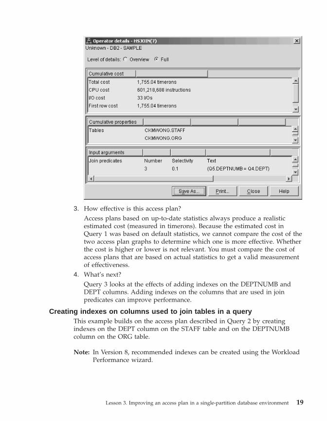
2. Does this access plan use the most effective methods of accessing data?Like Query 1, the access plan in Query 2 uses table scans (TBSCAN) notindex scans (IXSCAN). Even though current statistics exist, an index scanwas not done because there are no indexes on the columns that were usedby the query. One way to improve the query would be to provide theoptimizer with indexes on columns that are used to join tables (that is, oncolumns that are used in join predicates). In this example, this is the firstmerge scan join: HSJOIN (7).
Lesson 3. Improving an access plan in a single-partition database environment 17

In the Operator Details window for the HSJOIN (7) operator, look at theJoin predicates section under Input arguments. The columns used in thisjoin operation are listed under the Text column. In this example, thesecolumns are DEPTNUMB and DEPT.
18 VE Tutorial
3. How effective is this access plan?Access plans based on up-to-date statistics always produce a realisticestimated cost (measured in timerons). Because the estimated cost inQuery 1 was based on default statistics, we cannot compare the cost of thetwo access plan graphs to determine which one is more effective. Whetherthe cost is higher or lower is not relevant. You must compare the cost ofaccess plans that are based on actual statistics to get a valid measurementof effectiveness.
4. What’s next?Query 3 looks at the effects of adding indexes on the DEPTNUMB andDEPT columns. Adding indexes on the columns that are used in joinpredicates can improve performance.
Creating indexes on columns used to join tables in a queryThis example builds on the access plan described in Query 2 by creatingindexes on the DEPT column on the STAFF table and on the DEPTNUMBcolumn on the ORG table.
Note: In Version 8, recommended indexes can be created using the WorkloadPerformance wizard.
Lesson 3. Improving an access plan in a single-partition database environment 19

To view the access plan graph for this query (Query 3): in the ExplainedStatements History window, double-click the entry identified as QueryNumber 3. The Access Plan Graph window for this execution of the statementopens.
Note: Even though an index was created for DEPTNUM, the optimizer didnot use it.
Answering the following questions will help you understand how to improvethe query.1. What has changed in the access plan with indexes?
A nested loop join, NLJOIN (7), has replaced the merge scan join HSJOIN(7) that was used in Query 2. Using a nested loop join resulted in a lowerestimated cost than a merge scan join because this type of join does notrequire any sort or temporary tables.
20 VE Tutorial

A new diamond-shaped node, I_DEPT, has been added just above theSTAFF table. This node represents the index that was created on DEPT,and it shows that the optimizer used an index scan instead of a table scanto determine which rows to retrieve.
In this portion of the access plan graph, notice that a new index (I_DEPT)was created on the DEPT column and IXSCAN (17) was used to access theSTAFF table. In Query 2, a table scan was used to access the STAFF table.
2. Does this access plan use the most effective methods of accessing data?As a result of adding indexes, an IXSCAN node, IXSCAN (17), was usedto access the STAFF table. Query 2 did not have an index; therefore, atable scan was used in that example.The FETCH node, FETCH (11), shows that in addition to using the indexscan to retrieve the column DEPT, the optimizer retrieved additionalcolumns from the STAFF table, using the index as a pointer. In this case,the combination of index scan and fetch is calculated to be less costly thanthe full table scan used in the previous access plans.
Lesson 3. Improving an access plan in a single-partition database environment 21
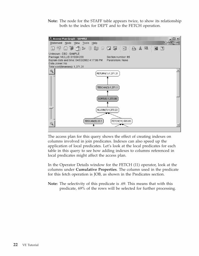
Note: The node for the STAFF table appears twice, to show its relationshipboth to the index for DEPT and to the FETCH operation.
The access plan for this query shows the effect of creating indexes oncolumns involved in join predicates. Indexes can also speed up theapplication of local predicates. Let’s look at the local predicates for eachtable in this query to see how adding indexes to columns referenced inlocal predicates might affect the access plan.
In the Operator Details window for the FETCH (11) operator, look at thecolumns under Cumulative Properties. The column used in the predicatefor this fetch operation is JOB, as shown in the Predicates section.
Note: The selectivity of this predicate is .69. This means that with thispredicate, 69% of the rows will be selected for further processing.
22 VE Tutorial
Lesson 3. Improving an access plan in a single-partition database environment 23
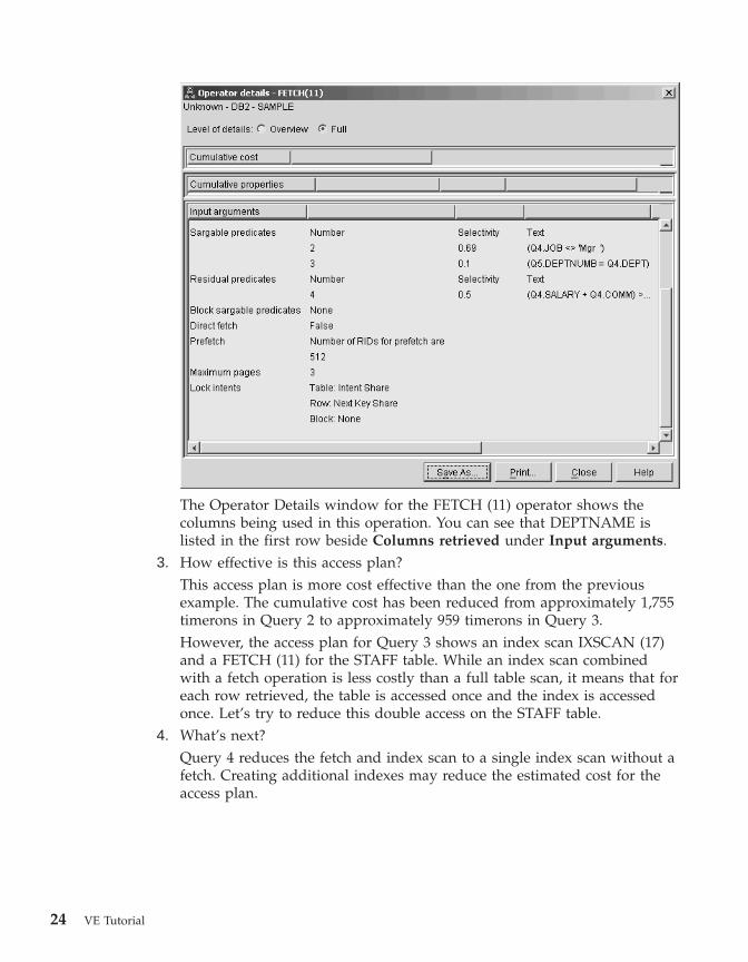
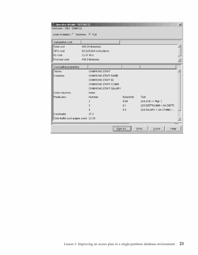
The Operator Details window for the FETCH (11) operator shows thecolumns being used in this operation. You can see that DEPTNAME islisted in the first row beside Columns retrieved under Input arguments.
3. How effective is this access plan?This access plan is more cost effective than the one from the previousexample. The cumulative cost has been reduced from approximately 1,755timerons in Query 2 to approximately 959 timerons in Query 3.However, the access plan for Query 3 shows an index scan IXSCAN (17)and a FETCH (11) for the STAFF table. While an index scan combinedwith a fetch operation is less costly than a full table scan, it means that foreach row retrieved, the table is accessed once and the index is accessedonce. Let’s try to reduce this double access on the STAFF table.
4. What’s next?Query 4 reduces the fetch and index scan to a single index scan without afetch. Creating additional indexes may reduce the estimated cost for theaccess plan.
24 VE Tutorial
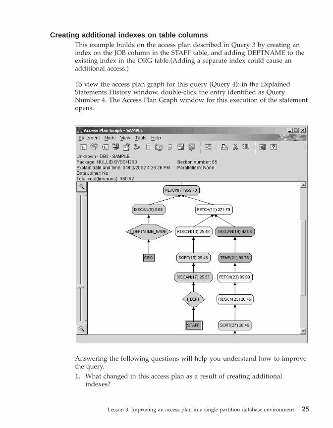
Creating additional indexes on table columnsThis example builds on the access plan described in Query 3 by creating anindex on the JOB column in the STAFF table, and adding DEPTNAME to theexisting index in the ORG table.(Adding a separate index could cause anadditional access.)
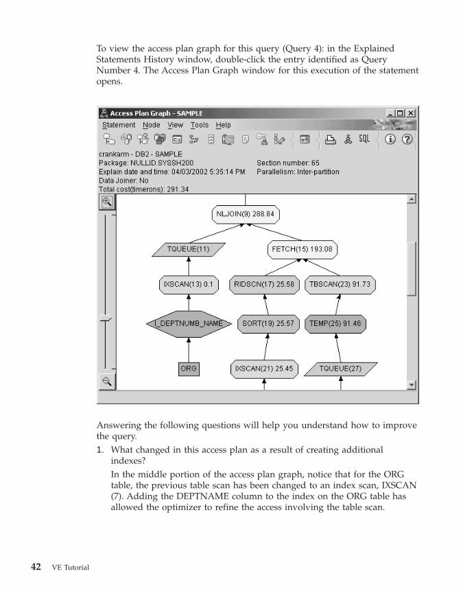
To view the access plan graph for this query (Query 4): in the ExplainedStatements History window, double-click the entry identified as QueryNumber 4. The Access Plan Graph window for this execution of the statementopens.
Answering the following questions will help you understand how to improvethe query.1. What changed in this access plan as a result of creating additional
indexes?
Lesson 3. Improving an access plan in a single-partition database environment 25

The optimizer has taken advantage of the index created on the JOBcolumn in the STAFF table (represented by a diamond labeled I_JOB) tofurther refine this access plan.
In the middle portion of the access plan graph, notice that for the ORGtable, the previous index scan and fetch have been changed to an indexscan only IXSCAN (9). Adding the DEPTNAME column to the index onthe ORG table has allowed the optimizer to eliminate the extra accessinvolving the fetch.
26 VE Tutorial

2. How effective is this access plan?This access plan is more cost effective than the one from the previousexample. The cumulative cost has been reduced from approximately 1,370timerons in Query 3 to approximately 959 timerons in Query 4.
What’s Next
Refer to the Administration Guide to find detailed information on additionalsteps that you can take to improve performance. You can then return to VisualExplain to assess the impact of your actions.
Lesson 3. Improving an access plan in a single-partition database environment 27

28 VE Tutorial

Lesson 4. Improving an access plan in a partitioneddatabase environment
In this lesson, you will learn how the access plan and related windows for thebasic query change when you perform various tuning activities. Using a seriesof examples, accompanied by illustrations, you will learn how the estimatedtotal cost for the access plan of even a simple query can be improved by usingthe runstats command and adding appropriate indexes.
As you gain experience with Visual Explain, you will discover other ways totune queries.
Working with access plan graphs
Using the four sample explain snapshots as examples, you will learn howtuning is an important part of database performance.
The queries associated with the explain snapshots are numbered 1 – 4. Eachquery uses the same SQL statement (described in Lesson 1):SELECT S.ID,S.NAME,O.DEPTNAME,SALARY+COMMFROM ORG O, STAFF SWHERE
O.DEPTNUMB = S.DEPT ANDS.JOB <> ’Mgr’ ANDS.SALARY+S.COMM > ALL( SELECT ST.SALARY*.9
FROM STAFF STWHERE ST.JOB=’Mgr’ )
ORDER BY S.NAME
But each iteration of the query uses more tuning technics than the previousexecution. For example, Query 1 has had no performance tuning, while Query4 has had the most. The differences in the queries are described below:
Query 1Running a query with no indexes and no statistics
Query 2Collecting current statistics for the tables and indexes in a query
Query 3Creating indexes on columns used to join tables in a query
Query 4Creating additional indexes on table columns
© Copyright IBM Corp. 2000 - 2002 29
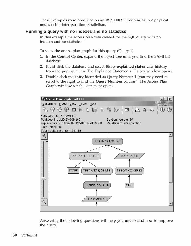
These examples were produced on an RS/6000 SP machine with 7 physicalnodes using inter-partition parallelism.
Running a query with no indexes and no statisticsIn this example the access plan was created for the SQL query with noindexes and no statistics.
To view the access plan graph for this query (Query 1):1. In the Control Center, expand the object tree until you find the SAMPLE
database.2. Right-click the database and select Show explained statements history
from the pop-up menu. The Explained Statements History window opens.3. Double-click the entry identified as Query Number 1 (you may need to
scroll to the right to find the Query Number column). The Access PlanGraph window for the statement opens.
Answering the following questions will help you understand how to improvethe query.
30 VE Tutorial

1. Do current statistics exist for each table in the query?To check if current statistics exist for each table in the query, double-clickon each table node in the access plan graph. In the corresponding TableStatistics window that opens, the STATS_TIME row under the Explainedcolumn contains the words ″Statistics not updated″ indicating that nostatistics had been collected at the time when the snapshot was created.If current statistics do not exist, the optimizer uses default statistics, whichmay differ from the actual statistics. Default statistics are identified by theword ″default″ under the Explained column in the Table Statistics window.According to the information in the Table Statistics window for the ORGtable, the optimizer used default statistics (as indicated next to theexplained values). Default statistics were used because actual statisticswere not available when the snapshot was created (as indicated in theSTATS_TIME row).
2. Does this access plan use the most effective methods of accessing data?This access plan contains table scans, not index scans. Table scans areshown as octagons and are labeled TBSCAN. If Index scans had been usedthey would appear as diamonds and be labeled IXSCAN. The use of anindex that was created for a table is more cost-effective than a table scan ifsmall amounts of data are being extracted.
3. How effective is this access plan?
Lesson 4. Improving an access plan in a partitioned database environment 31

You can determine the effectiveness of an access plan only if it is based onactual statistics. Since the optimizer used default statistics in the accessplan, you cannot determine how effective the plan is.In general, you should make a note of the total estimated cost for theaccess plan for later comparison with revised access plans. The cost listedin each node is cumulative, from the first steps of your query up to andincluding the node.
Note: For partitioned databases, this is the cumulative cost for the nodethat uses the most resources.
In the Access Plan Graph window, the total cost is approximately 1,234timerons, shown in RETURN (1) at the top of the graph. The totalestimated cost is also shown in the top area of the window.
4. What’s next?
32 VE Tutorial
Query 2 looks at an access plan for the basic query after runstats has beenrun. Using the runstats command provides the optimizer with currentstatistics on all tables accessed by the query.
Collecting current statistics for the tables and indexes using runstatsThis example builds on the access plan described in Query 1 by collectingcurrent statistics with the runstats command.
It is highly recommended that you use the runstats command to collectcurrent statistics on tables and indexes, especially if significant update activityhas occurred or new indexes have been created since the last time the runstatscommand was executed. This provides the optimizer with the most accurateinformation with which to determine the best access plan. If current statisticsare not available, the optimizer can choose an inefficient access plan based oninaccurate default statistics.
Be sure to use runstats after making your table updates; otherwise, the tablemay appear to the optimizer to be empty. This problem is evident ifcardinality on the Operator Details window equals zero. In this case, completeyour table updates, rerun the runstats command, and recreate the explainsnapshots for affected tables.
To view the access plan graph for this query (Query 2): in the ExplainedStatements History window, double-click the entry identified as QueryNumber 2. The Access Plan Graph window for this execution of the statementopens.
Lesson 4. Improving an access plan in a partitioned database environment 33
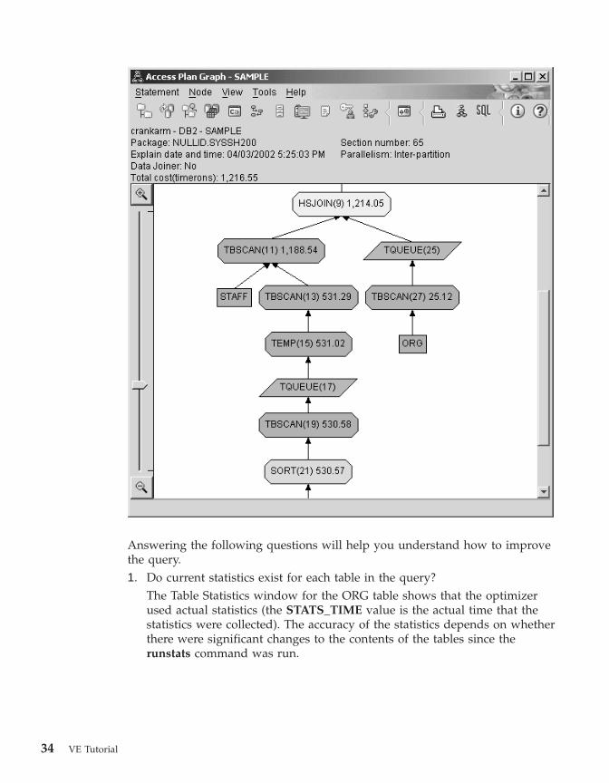
Answering the following questions will help you understand how to improvethe query.1. Do current statistics exist for each table in the query?
The Table Statistics window for the ORG table shows that the optimizerused actual statistics (the STATS_TIME value is the actual time that thestatistics were collected). The accuracy of the statistics depends on whetherthere were significant changes to the contents of the tables since therunstats command was run.
34 VE Tutorial

2. Does this access plan use the most effective methods of accessing data?Like Query 1, the access plan in Query 2 uses table scans (TBSCAN) notindex scans (IXSCAN). Even though current statistics exist, an index scanwas not done because there are no indexes on the columns that were usedby the query. One way to improve the query would be to provide theoptimizer with indexes on columns that are used to join tables (that is, oncolumns that are used in join predicates). In this example, this is the firstmerge scan join: HSJOIN (9).
Lesson 4. Improving an access plan in a partitioned database environment 35

In the Operator Details window for the HSJOIN (9) operator, look at theJoin predicates section under Input arguments. The columns used in thisjoin operation are listed under the Text column. In this example, thesecolumns are DEPTNUMB and DEPT.
36 VE Tutorial

3. How effective is this access plan?Access plans based on up-to-date statistics always produce a realisticestimated cost (measured in timerons). Because the estimated cost inQuery 1 was based on default statistics, we cannot compare the cost of thetwo access plan graphs to determine which one is more effective. Whetherthe cost is higher or lower is not relevant. You must compare the cost ofaccess plans that are based on actual statistics to get a valid measurementof effectiveness.
4. What’s next?Query 3 looks at the effects of adding indexes on the DEPTNUMB andDEPT columns. Adding indexes on the columns that are used in joinpredicates can improve performance.
Creating indexes on columns used to join tables in a queryThis example builds on the access plan described in Query 2 by creatingindexes on the DEPT column on the STAFF table and on the DEPTNUMBcolumn on the ORG table.
Note: In Version 8, recommended indexes can be created using the WorkloadPerformance wizard.
Lesson 4. Improving an access plan in a partitioned database environment 37

To view the access plan graph for this query (Query 3): in the ExplainedStatements History window, double-click the entry identified as QueryNumber 3. The Access Plan Graph window for this execution of the statementopens.
Note: Even though an index was created for DEPTNUM, the optimizer didnot use it.
Answering the following questions will help you understand how to improvethe query.1. What has changed in the access plan with indexes?
38 VE Tutorial

A new diamond-shaped node, I_DEPT, has been added just above theSTAFF table. This node represents the index that was created on DEPT,and it shows that the optimizer used an index scan instead of a table scanto determine which rows to retrieve.
2. Does this access plan use the most effective methods of accessing data?The access plan for this query shows the effect of creating indexes on theDEPTNUMB column of the ORG table, resulting in FETCH (15) andIXSCAN (21) and on the DEPT column of the STAFF table. Query 2 didnot have this index; therefore, a table scan was used in that example.
Lesson 4. Improving an access plan in a partitioned database environment 39

The Operator Details window for the FETCH(15) operator shows thecolumns being used in this operation.
40 VE Tutorial

The combination of index and fetch are calculated to be less costly thanthe full table scan used in the previous access plans.
3. How effective is this access plan?This access plan is more cost effective than the one from the previousexample. The cumulative cost has been reduced from approximately 1,214timerons in Query 2 to approximately 755 timerons in Query 3.
4. What’s next?Query 4 reduces the fetch and index scan to a single index scan without afetch. Creating additional indexes may reduce the estimated cost for theaccess plan.
Creating additional indexes on table columnsThis example builds on the access plan described in Query 3 by creating anindex on the JOB column in the STAFF table, and adding DEPTNAME to theexisting index in the ORG table.(Adding a separate index could cause anadditional access.)
Lesson 4. Improving an access plan in a partitioned database environment 41
To view the access plan graph for this query (Query 4): in the ExplainedStatements History window, double-click the entry identified as QueryNumber 4. The Access Plan Graph window for this execution of the statementopens.
Answering the following questions will help you understand how to improvethe query.1. What changed in this access plan as a result of creating additional
indexes?In the middle portion of the access plan graph, notice that for the ORGtable, the previous table scan has been changed to an index scan, IXSCAN(7). Adding the DEPTNAME column to the index on the ORG table hasallowed the optimizer to refine the access involving the table scan.
42 VE Tutorial

In the bottom portion of the access plan graph, note that for the STAFFtable the previous index scan and fetch have been changed to an indexscan only IXSCAN (39). Creating the JOB index on the STAFF table hasallowed the optimizer to eliminate the extra access involving the fetch.
Lesson 4. Improving an access plan in a partitioned database environment 43

2. How effective is this access plan?This access plan is more cost effective than the one from the previousexample. The cumulative cost has been reduced from approximately 753timerons in Query 3 to approximately 288 timerons in Query 4.
44 VE Tutorial
What’s Next
Refer to the Administration Guide to find detailed information on additionalsteps that you can take to improve performance. You can then return to VisualExplain to assess the impact of your actions.
Lesson 4. Improving an access plan in a partitioned database environment 45

46 VE Tutorial

Appendix A. Visual Explain concepts
Access plan
Certain data is necessary to resolve an explainable SQL statement. An accessplan specifies an order of operations for accessing this data. It lets you viewstatistics for selected tables, indexes, or columns; properties for operators;global information such as table space and function statistics; andconfiguration parameters relevant to optimization. With Visual Explain, youcan view the access plan for an SQL statement in graphical form.
The optimizer produces an access plan whenever an explainable SQLstatement is compiled. This happens at prep/bind time for static statements,and at run time for dynamic statements.
It is important to understand that an access plan is an estimate based on theinformation that is available. The optimizer bases its estimations oninformation such as the following:v Statistics in system catalog tables (if statistics are not current, update them
using the runstats command.)v Configuration parametersv Bind optionsv The query optimization class
Cost information associated with an access plan is the optimizer’s best estimateof the resource usage for a query. The actual elapsed time for a query mayvary depending on factors outside the scope of DB2 (for example, the numberof other applications running at the same time). Actual elapsed time can bemeasured while running the query, by using performance monitoring.
Access plan graph
Visual Explain uses information from a number of sources in order to producean access plan graph, as shown in the illustration below. Based on variousinputs, the optimizer chooses an access plan, and Visual Explain displays it inan access plan graph. The nodes in the graph represent tables and indexes andeach operation on them. The links between the nodes represent the flow of
© Copyright IBM Corp. 2000 - 2002 47

data.
DB2
Control Center
9. Accessplan graph
Optimizer
7. Access plan
Query Execution
5. Prep/BindOptions
6. Query
1. Tables2. Indexes3. Statistics4. Configuration
Parameters
8. ExplainSnapshot
VisualExplain
The following list of tasks correspond to those shown in the illustration above.(Broken lines indicate steps that are required for Visual Explain.)1. Tune your table design and reorganize table data.2. Create appropriate indexes.3. Use the runstats command to provide the optimizer with current statistics.4. Choose appropriate configuration parameters.5. Choose appropriate bind options.6. Design queries to retrieve only required data .7. Create an access plan.8. Create explain snapshots.9. Display and use an access plan graph.
For example, to use Visual Explain, first update current statistics using therunstats command on the tables, and indexes used by the statement. Thesestatistics, the configuration parameters, bind options, and the query itself areused by the optimizer to create an access plan and an explain snapshot whenthe package is bound. Visual Explain uses the resulting explain snapshot todisplay the access plan graph for the statement.
Access plan graph node
The access plan graph consists of a tree displaying nodes. These nodesrepresent:v Tables, shown as rectanglesv Indexes, shown as diamondsv Operators, shown as octagons (8 sides). TQUEUE operators, shown as
parallelograms
48 VE Tutorial

v Table functions, shown as hexagons(6 sides).
Clustering
Over time, updates may cause rows on data pages to change locationlowering the degree of clustering that exists between an index and the datapages. Reorganizing a table with respect to a chosen index reclusters the data.A clustered index is most useful for columns that have range predicatesbecause it allows better sequential access of data in the base table. This resultsin fewer page fetches, since like values are on the same data page.
In general, only one of the indexes in a table can have a high degree ofclustering.
To check the degree of clustering for an index, double-click on its node todisplay the Index Statistics window. The cluster ratio or cluster factor valuesare shown in this window. If the value is low, consider reorganizing thetable’s data.
For more information, see the section on reorganizing table data in theAdministration Guide.
Container
A container is a physical storage location of the data. It is associated with atable space, and can be a file or a directory or a device.
Cost
Cost, in the context of Visual Explain, is the estimated total resource usagenecessary to execute the access plan for a statement (or the elements of astatement). Cost is derived from a combination of CPU cost (in number ofinstructions) and I/O (in numbers of seeks and page transfers).
The unit of cost is the timeron. A timeron does not directly equate to anyactual elapsed time, but gives a rough relative estimate of the resources (cost)required by the database manager to execute two plans for the same query.
The cost shown in each operator node of an access plan graph is thecumulative cost, from the start of access plan execution up to and includingthe execution of that particular operator. It does not reflect factors such as theworkload on the system or the cost of returning rows of data to the user.
Appendix A. Visual Explain concepts 49

Cursor blocking
Cursor blocking is a technique that reduces overhead by having the databasemanager retrieve a block of rows in a single operation. These rows are storedin a cache while they are processed. The cache is allocated when anapplication issues an OPEN CURSOR request, and is deallocated when thecursor is closed. When all the rows have been processed, another block ofrows is retrieved.
Use the BLOCKING option on the PREP or BIND commands along with thefollowing parameters to specify the type of cursor blocking:
UNAMBIGOnly unambiguous cursors are blocked (the default).
ALL Both ambiguous and unambiguous cursors are blocked.
NO Cursors are not blocked.
For more information, see the section on cursor blocking in the AdministrationGuide.
Database-managed space (DMS) table space
There are two types of table spaces that can exist in a database:Database-managed space (DMS), and system-managed space (SMS).
DMS table spaces are managed by the database manager. and are designedand tuned to meet its requirements.
The DMS table space definition includes a list of files (or devices) into whichthe database data is stored in its DMS table space format.
You can add pre-allocated files (or devices) to an existing DMS table space inorder to increase its storage capacity. The database manager automaticallyrebalances existing data in all the containers belonging to that table space.
DMS and SMS table spaces can coexist in the same database.
Dynamic SQL
Dynamic SQL statements are SQL statements that are prepared and executedwithin an application program while the program is running. In dynamicSQL, either:v You issue the SQL statement interactively, using CLI or CLPv The SQL source is contained in host language variables that are embedded
in an application program.
50 VE Tutorial
When DB2 runs a dynamic SQL statement, it creates an access plan that isbased on current catalog statistics and configuration parameters. This accessplan might change from one execution of the statements application programto the next.
The alternative to dynamic SQL is static SQL.
Explain snapshot
With Visual Explain, you can examine the contents of an explain snapshot.
An explain snapshot is compressed information that is collected when an SQLstatement is explained. It is stored as a binary large object (BLOB) in theEXPLAIN_STATEMENT table, and contains the following information:v The internal representation of the access plan, including its operators and
the tables and indexes accessedv The decision criteria used by the optimizer, including statistics for database
objects and the cumulative cost for each operation.
An explain snapshot is required if you want to display the graphicalrepresentation of an SQL statement’s access plan. To ensure that an explainsnapshot is created:1. Explain tables must exist in the database manager to store the explain
snapshots. For information on how to create these tables, see Creatingexplain tables in the online help.
2. For a package containing static SQL statements, set the EXPLSNAP optionto ALL or YES when you bind or prep the package. You will get anexplain snapshot for each explainable SQL statement in the package. Formore information on the BIND and PREP commands, see the CommandReference.
3. For dynamic SQL statements, set the EXPLSNAP option to ALL when youbind the application that issues them, or set the CURRENT EXPLAINSNAPSHOT special register to YES or EXPLAIN before you issue theminteractively. For more information, see the section on current explainsnapshots in the SQL Reference.
Explainable statement
An explainable statement is an SQL statement for which an explain operationcan be performed.
Explainable SQL statements are:v SELECTv INSERTv UPDATE
Appendix A. Visual Explain concepts 51

v DELETEv VALUES
Explained statement
An explained statement is an SQL statement for which an explain operation hasbeen performed. Explained statements are shown in the Explained StatementsHistory window.
Operand
An operand is an entity on which an operation is performed. For example, atable or an index is an operand of various operators such as TBSCAN andIXSCAN.
Operator
An operator is either an action that must be performed on data, or the outputfrom a table or an index, when the access plan for an SQL statement isexecuted.
The following operators can appear in the access plan graph:
DELETEDeletes rows from a table.
EISCANScans a user defined index to produce a reduced stream of rows.
FETCHFetches columns from a table using a specific record identifier.
FILTERFilters data by applying one or more predicates to it.
GRPBYGroups rows by common values of designated columns or functions,and evaluates set functions.
HSJOINRepresents a hash join, where two or more tables are hashed on thejoin columns.
INSERTInserts rows into a table.
IXANDANDs together the row identifiers (RIDs) from two or more indexscans.
52 VE Tutorial

IXSCANScans an index of a table with optional start/stop conditions,producing an ordered stream of rows.
MSJOINRepresents a merge join, where both outer and inner tables must be injoin-predicate order.
NLJOINRepresents a nested loop join that accesses an inner table once foreach row of the outer table.
RETURNRepresents the return of data from the query to the user.
RIDSCNScans a list of row identifiers (RIDs) obtained from one or moreindexes.
SHIP Retrieves data from a remote database source. Used in the federatedsystem.
SORT Sorts rows in the order of specified columns, and optionallyeliminates duplicate entries.
TBSCANRetrieves rows by reading all required data directly from the datapages.
TEMP Stores data in a temporary table to be read back out (possibly multipletimes).
TQUEUETransfers table data between database agents.
UNIONConcatenates streams of rows from multiple tables.
UNIQUEEliminates rows with duplicate values, for specified columns.
UPDATEUpdates rows in a table.
CMPEXP
Operator name: CMPEXP
Represents: The computation of expressions required for intermediate or finalresults.
(This operator is for debug mode only.)
Appendix A. Visual Explain concepts 53

DELETE
Operator name: DELETE
Represents: The deletion of rows from a table.
This operator represents a necessary operation. To improve access plan costs,concentrate on other operators (such as scans and joins) that define the set ofrows to be deleted.
Performance Suggestion:
v If you are deleting all rows from a table, consider using the DROP TABLEstatement or the LOAD REPLACE command.
EISCAN
Operator name: EISCAN
Represents: This operator scans a user defined index to produce a reducedstream of rows. The scanning uses the multiple start/stop conditions from theuser supplied range producer function.
This operation is performed to narrow down the set of qualifying rows beforeaccessing the base table (based on predicates).
Performance Suggestion:
v Over time, database updates may cause an index to become fragmented,resulting in more index pages than necessary. This can be corrected bydropping and recreating the index, or reorganizing the index.
v If statistics are not current, update them using the runstats command.
FETCH
Operator name: FETCH
Represents: The fetching of columns from a table using a specific rowidentifier (RID).
Performance suggestions:
v Expand index keys to include the fetched columns so that the data pagesdo not have to be accessed.
v Find the index related to the fetch, and double-click on its node to displayits statistics window. Ensure that the degree of clustering is high for theindex.
54 VE Tutorial

v Increase the buffer size if the input/output (I/O) incurred by the fetch isgreater than the number of pages in the table.
v If statistics are not current, update them using the runstats command.The quantile and frequent value statistics provide information on theselectivity of predicates, which determines when index scans are chosenover table scans. To update these statistics, use the runstats command on atable with the WITH DISTRIBUTION clause.
FILTER
Operator name: FILTER
Represents: The application of residual predicates so that data is filteredbased on the criteria supplied by the predicates.
Performance suggestions:
v Ensure that you have used predicates that retrieve only the data you need.For example, ensure that the selectivity value for the predicates representsthe portion of the table that you want returned.
v Ensure that the optimization class is at least 3 so that the optimizer uses ajoin instead of a subquery. If this is not possible, try rewriting the SQLquery by hand to eliminate the subquery. For an example, see the sectionon query rewrites by the SQL compiler in the Administration Guide.
GENROW
Operator name: GENROW
Represents: A built-in function that generates a table of rows, using no inputfrom tables, indexes, or operators.
GENROW may be used by the optimizer to generate rows of data (forexample, for an INSERT statement or for some IN-lists that are transformedinto joins).
To view the estimated statistics for the tables generated by the GENROWfunction, double-click on its node.
GRPBY
Operator name: GRPBY
Represents: The grouping of rows according to common values of designatedcolumns or functions. This operation is required to produce a group of values,or to evaluate set functions.
Appendix A. Visual Explain concepts 55

If no GROUP BY columns are specified, the GRPBY operator may still be usedif there are aggregation functions in the SELECT list, indicating that the entiretable is treated as a single group when doing that aggregation.
Performance suggestions:
v This operator represents a necessary operation. To improve access plancosts, concentrate on other operators (such as scans and joins) that definethe set of rows to be grouped.
v To improve the performance of a SELECT statement that contains a singleaggregate function but no GROUP BY clause, try the following:– For a MIN(C) aggregate function, create an ascending index on C.– For a MAX(C) aggregate function, create a descending index on C.
HSJOIN
Operator name: HSJOIN
Represents: A hash join for which the qualified rows from tables are hashedto allow direct joining, without pre-ordering the content of the tables.
A join is necessary whenever there is more than one table referenced in aFROM clause. A hash join is possible whenever there is a join predicate thatequates columns from two different tables. The join predicates need to beexactly the same data type. Hash joins may also arise from a rewrittensubquery, as is the case with NLJOIN.
A hash join does not require the input tables be ordered. The join isperformed by scanning the inner table of the hash join and generating alookup table by hashing the join column values. It then reads the outer table,hashing the join column values, and checking in the lookup table generatedfor the inner table.
For more information, see the section on join concepts in the AdministrationGuide.
Performance suggestions:
v Use local predicates (that is, predicates that reference one table) to reducethe number of rows to be joined.
v Increase the size of the sort heap to make it large enough to hold the hashlookup table in memory.
v If statistics are not current, update them using the runstats command.
56 VE Tutorial

INSERT
Operator name: INSERT
Represents: The insertion of rows into a table.
This operator represents a necessary operation. To improve access plan costs,concentrate on other operators (such as scans and joins) that define the set ofrows to be inserted.
IXAND
Operator name: IXAND
Represents: The ANDing of the results of multiple index scans using DynamicBitmap techniques. The operator allows ANDed predicates to be applied tomultiple indexes, in order to reduce underlying table accesses to a minimum.
This operator is performed to:v Narrow down the set of rows before accessing the base tablev AND together predicates applied to multiple indexesv AND together the results of semijoins, used in star joins.
Performance suggestions:
v Over time, database updates may cause an index to become fragmented,resulting in more index pages than necessary. This can be corrected bydropping and recreating the index, or reorganizing the index.
v If statistics are not current, update them using the runstats command.v In general, index scans are most effective when only a few rows qualify. To
estimate the number of qualifying rows, the optimizer uses the statisticsthat are available for the columns referenced in predicates. If some valuesoccur more frequently than others, it is important to request distributionstatistics by using the WITH DISTRIBUTION clause for the runstatscommand. By using the non-uniform distribution statistics, the optimizercan distinguish among frequently and infrequently occurring values.
v IXAND can best exploit single column indexes, as start and stop keys arecritical in the use of IXAND.
v For star joins, create single-column indexes for each of the most selectivecolumns in the fact table and the related dimension tables.
IXSCAN
Operator name: IXSCAN
Appendix A. Visual Explain concepts 57

Represents: The scanning of an index to produce a reduced stream of rows.The scanning can use optional start/stop conditions, or may apply toindexable predicates that reference columns of the index.
This operation is performed to narrow down the set of qualifying rows beforeaccessing the base table (based on predicates).
For more information, see the section on index scans in the AdministrationGuide.
Performance suggestions:
v Over time, database updates may cause an index to become fragmented,resulting in more index pages than necessary. This can be corrected bydropping and recreating the index, or reorganizing the index.
v When two or more tables are being accessed, access to the inner table viaan index may be made more efficient by providing an index on the joincolumn of the outer table.For more guidelines about indexes, see the online help for Visual Explain.
v If statistics are not current, update them using the runstats command.v In general, index scans are most effective when only a few rows qualify. To
estimate the number of qualifying rows, the optimizer uses the statisticsthat are available for the columns referenced in predicates. If some valuesoccur more frequently than others, it is important to request distributionstatistics by using the WITH DISTRIBUTION clause for the runstatscommand. By using the non-uniform distribution statistics, the optimizercan distinguish among frequently and infrequently occurring values.
MSJOIN
Operator name: MSJOIN
Represents: A merge join for which the qualified rows from both outer andinner tables must be in join-predicate order. A merge join is also called a mergescan join or a sorted merge join.
A join is necessary whenever there is more than one table referenced in aFROM clause. A merge join is possible whenever there is a join predicate thatequates columns from two different tables. It may also arise from a rewrittensubquery.
A merge join requires ordered input on joining columns, since the tables aretypically scanned only once. This ordered input is obtained by accessing anindex or a sorted table.
58 VE Tutorial
For more information, see the section on join concepts in the AdministrationGuide.
Performance suggestions:
v Use local predicates (that is, predicates that reference one table) to reducethe number of rows to be joined.For guidelines about indexes, see Creating appropriate indexes in the onlinehelp for Visual Explain.
v If statistics are not current, update them using the runstats command.
NLJOIN
Operator name: NLJOIN
Represents: A nested loop join that scans (usually with an index scan) theinner table once for each row of the outer table.
A join is necessary whenever there is more than one table referenced in aFROM clause. A nested loop join does not require a join predicate, butgenerally performs better with one.
A nested loop join is performed either:v By scanning through the inner table for each accessed row of the outer
table.v By performing an index lookup on the inner table for each accessed row of
the outer table.
For more information, see the section on join concepts in the AdministrationGuide.
Performance suggestions:
v A nested loop join is likely to be more efficient if there is an index on thejoin-predicate columns of the inner table (the table displayed to the right ofthe NLJOIN operator). Check to see if the inner table is a TBSCAN ratherthan an IXSCAN. If it is, consider adding an index on its join columns.Another (less important) way to make the join more efficient is to create anindex on the join columns of the outer table so that the outer table isordered.For more guidelines about indexes, see Creating appropriate indexes in theonline help for Visual Explailn.
v If statistics are not current, update them using the runstats command.
Related information:
v Star Joins.
Appendix A. Visual Explain concepts 59

PIPE
Operator name: PIPE
Represents: The transfer of rows to other operators without any change to therows.
(This operator is for debug mode only.)
RETURN
Operator name: RETURN
Represents: The return of data from a query to the user. This is the finaloperator in the access plan graph and shows the total accumulated values andcosts for the access plan.
This operator represents a necessary operation.
Performance Suggestion:
v Ensure that you have used predicates that retrieve only the data you need.For example, ensure that the selectivity value for the predicates representsthe portion of the table that you want returned.
RIDSCN
Operator name: RIDSCN
Represents: The scan of a list of row identifiers (RIDs) obtained from one ormore indexes.
This operator is considered by the optimizer when:v Predicates are connected by OR keywords, or there is an IN predicate. A
technique called index ORing can be used, which combines results frommultiple index accesses on the same table.
v It is beneficial to use list prefetch for a single index access, since sorting therow identifiers before accessing the base rows makes the I/O more efficient.
RQUERY
Operator name: SHIP
Represents: An operator used in the federated system to retrieve data from aremote data source. This operator is considered by the optimizer when: ASHIP operator sends a SQL SELECT statement to a remote data source to
60 VE Tutorial
retrieve the query result. The SELECT statement is generated using the SQLdialect supported by the data source, and can contain any valid query asallowed by the data source.
Performance Suggestion: Refer to Chapter 4 in the Administration Guide Vol2, Federated Database Query and Network Tuning Information.
SORT
Operator name: SORT
Represents: The sorting of the rows in a table into the order of one or more ofits columns, optionally eliminating duplicate entries.
Sorting is required when no index exists that satisfies the requested ordering,or when sorting would be less expensive than an index scan. Sorting isusually performed as a final operation once the required rows are fetched, orto sort data prior to a join or a group by.
If the number of rows is high or if the sorted data cannot be piped, theoperation requires the costly generation of temporary tables.
For more information on sorts, see the Administration Guide.
Performance suggestions:
v Consider adding an index on the sort columns.For guidelines about indexes, see Creating appropriate indexes in the onlinehelp for Visual Explain.
v Ensure that you have used predicates that retrieve only the data you need.For example, ensure that the selectivity value for the predicates representsthe portion of the table that you want returned.
v Check that the prefetch size of the system temporary table space isadequate, that is, it is not I/O bound. (To check this, selectStatement->Show statistics->Table spaces.)
v If frequent large sorts are required, consider increasing the values of thefollowing configuration parameters:– Sort heap size (sortheap). To change this parameter, right-click on the
database in the Control Center, and then select Configure from its pop-upmenu. Select the Performance tab from the notebook that appears.
– Sort heap threshold (sheapthres). To change this parameter, right-click onthe database instance in the Control Center, and then select Configurefrom its pop-up menu. Select the Performance tab from the notebookthat appears.
v If statistics are not current, update them using the runstats command.
Appendix A. Visual Explain concepts 61

TBSCAN
Operator name: TBSCAN
Represents: A table scan (relation scan) that retrieves rows by reading all therequired data directly from the data pages.
This type of scan is chosen by the optimizer over an index scan when:v The range of values scanned occurs frequently (that is, most of the table
must be accessed)v The table is smallv Index clustering is lowv An index does not exist
For more information on table and index scans, see the Administration Guide.
Performance suggestions:
v An index scan is more efficient than a table scan if the table is large, withmost of the table’s rows not being accessed. To increase the possibility thatan index scan will be used by the optimizer for this situation, consideradding indexes on columns for which there are selective predicates.For more guidelines about indexes, see Creating appropriate indexes in theonline help for Visual Explain.
v If an index already exists but was not used, check that there are selectivepredicates on each of its leading columns. If these predicates do exist, nextcheck that the degree of clustering is high for the index. (To see thisstatistic, open the Table Statistics window for the table beneath the sort, andselect its Indexes push button to bring up the the Index Statistics window.)
v Check that the prefetch size of the table space is adequate that is, it is notI/O bound. (To check this, select Statement->Show statistics->Tablespaces.)For more information, see the section on prefetching data into the bufferpool in the Administration Guide.
v If the statistics are not current, update them using the runstats command.The quantile and frequent value statistics provide information on theselectivity of predicates. For example, these statistics would be used todetermine when index scans are chosen over table scans. To update thesevalues, use the runstats command on a table with the WITHDISTRIBUTION clause.
TEMP
Operator name: TEMP
62 VE Tutorial

Represents: The action of storing data in a temporary table, to be read backout by another operator (possibly multiple times). The table is removed afterthe SQL statement is processed, if not before.
This operator is required to evaluate subqueries or to store intermediateresults. In some situations (such as when the statement can be updated), itmay be mandatory.
TQUEUE
Operator name: TQUEUE
Represents: A table queue that is used to pass table data from one databaseagent to another when there are multiple database agents processing a query.Multiple database agents are used to process a query when parallelism isinvolved.
Table queue types are:v Local: The table queue is used to pass data between database agents within
a single node. A local table queue is used for intra-partition parallelism.v Non-Local: The table queue is used to pass data between database agents
on different nodes.
UNION
Operator name: UNION
Represents: The concatenation of streams of rows from multiple tables.
This operator represents a necessary operation. To improve access plan costs,concentrate on other operators (such as scans and joins) that define the set ofrows to be concatenated.
UNIQUE
Operator name: UNIQUE
Represents: The elimination of rows having duplicate values for specifiedcolumns.
Performance Suggestion:
v This operator is not necessary only if a unique index exists on appropriatecolumns.For guidelines about indexes, see Creating appropriate indexes in the onlinehelp for Visual Explain.
Appendix A. Visual Explain concepts 63
UPDATE
Operator name: UPDATE
Represents: The updating of data in the rows of a table.
This operator represents a necessary operation. To improve access plan costs,concentrate on other operators (such as scans and joins) that define the set ofrows to be updated.
Optimizer
The optimizer is the component of the SQL compiler that chooses an accessplan for a data manipulation language (DML) SQL statement. It does this bymodeling the execution cost of many alternative access plans, and choosingthe one with the minimal estimated cost.
Package
A package is an object stored in the database that includes the informationneeded to process the SQL statements associated with one source file of anapplication program. It is generated by either:v Precompiling a source file with the PREP commandv Binding a bind file that was generated by the precompiler with the BIND
command.
Predicate
A predicate is an element of a search condition that expresses or implies acomparison operation. Predicates are included in clauses beginning withWHERE or HAVING.
For example, in the following SQL statement:SELECT * FROM SAMPLE
WHERE NAME = ’SMITH’ ANDDEPT = 895 AND YEARS > 5
The following are predicates: NAME = ’SMITH’; DEPT = 895; andYEARS > 5.
Predicates fall into one of the following categories, ordered from most efficientto least efficient:1. Starting and stopping conditions bracket (narrow down) an index scan.
(These conditions are also called range-delimiting predicates.)
64 VE Tutorial

2. Index-page (also known as index sargable) predicates can be evaluatedfrom an index because the columns involved in the predicate are part ofthe index key.
3. Data-page (also known as data sargable) predicates cannot be evaluatedfrom an index, but can be evaluated while rows remain in the buffer.
4. Residual predicates typically require I/O beyond the simple accessing of abase table, and must be applied after data is copied out of the buffer page.They include predicates that contain subqueries, or those that read LONGVARCHAR or LOB data stored in files separate from the table.
When designing predicates, you should aim for the highest selectivity possibleso that the fewest rows are returned.
The following types of predicates are the most effective and the mostcommonly used:v A simple equality join predicate is required for a merge join. It is of the form
table1.column = table2.column, and allows columns in two different tablesto be equated so that the tables can be joined.
v A local predicate is applied to one table only.
For more information, see the sections on data access concepts andoptimization in the Administration Guide.
Query optimization class
A query optimization class is a set of query rewrite rules and optimizationtechniques for compiling queries.
The primary query optimization classes are:
1 Restricted optimization. Useful when memory and processingresources are severely restrained. Roughly equivalent to theoptimization provided by Version 1.
2 Slight optimization. Specifies a level of optimization higher than thatof Version 1, but at significantly less optimization cost than levels 3and above, especially for very complex queries.
3 Moderate optimization. Comes closest to matching the queryoptimization characteristics of DB2 for MVS/ESA.
5 Normal optimization. Recommended for a mixed environment usingboth simple transactions and complex queries.
7 Normal optimization. The same as query optimization 5 except that itdoes not reduce the amount of query optimization for complexdynamic SQL queries.
Appendix A. Visual Explain concepts 65

Other query optimization classes, to be used only under special circumstances,are:
0 Minimal optimization. Use only when little or no optimization isrequired (that is, for very simple queries on well-indexed tables).
9 Maximum optimization. Uses substantial memory and processingresources. Use only if class 5 is insufficient (that is, for very complexand long-running queries that do not perform well at class 5).
In general, use a higher optimization class for static queries and for queriesthat you anticipate will take a long time to execute, and a lower optimizationclass for simple queries that are submitted dynamically or that are run only afew times.
To set the query optimization for dynamic SQL statements, enter the followingcommand in the Command Line Processor:SET CURRENT QUERY OPTIMIZATION = n;
where ’n’ is the desired query optimization class.
To set the query optimization for static SQL statements, use the QUERYOPToption on the BIND or PREP commands.
For more information, see the section on adjusting the optimization class inthe Administration Guide.
Selectivity of predicates
Selectivity refers to the probability that any row will satisfy a predicate (that is,be true).
For example, a selectivity of 0.01 (1%) for a predicate operating on a tablewith 1,000,000 rows means that the predicate returns an estimated 10,000 rows(1% of 1,000,000), and discards an estimated 990,000 rows.
A highly selective predicate (one with a selectivity of 0.10 or less) is desirable.Such predicates return fewer rows for future operators to work on, therebyrequiring less CPU and I/O to satisfy the query.
Example
Suppose that you have a table of 1,000,000 rows, and that the original querycontains an ’ORDER BY’ clause requiring an additional sorting step. With apredicate that has a selectivity of 0.01, the sort would have to be done on an
66 VE Tutorial

estimated 10,000 rows. However, with a less selective predicate of 0.50, thesort would have to be done on an estimated 500,000 rows, thus requiringmore CPU and I/O time.
Star joins
A set of joins are considered to be a star join when a fact table (large centraltable) is joined to two or more dimension tables (smaller tables containingdescriptions of the column values in the fact table).
A Star join is comprised of 3 main parts:v Semijoinsv Index ANDing of the results of the Semijoinsv Completing the semijoins.
It shows up as two or more joins feeding an IXAND operator.
A Semijoin is a special form of join in which the result of the join is only theRow Identifier (RID) of the inner table, instead of the joining of the inner andouter table columns.
Star joins use Semijoins to supply Row Identifiers to an Index ANDingoperator. The Index ANDing operator accumulates the filtering affect of thevarious joins. The output from the Index ANDing operator is fed into anIndex ORing operator, which orders the Row Identifiers, and eliminates anyduplicate rows that may have resulted from the joins feeding the IndexANDing operator. The rows from the fact table are then fetched, using a Fetchoperator. Finally, the reduced fact table is joined to all of the dimension tables,to complete the joins.
Performance suggestions:
v Create indexes on the fact table for each of the dimension table joins.v Ensure the sort heap threshold is high enough to allow allocating the Index
ANDing operator’s bit filter. For star joins, this could require as much as12MB, or 3000 4K pages. For Intra-partition parallelism, the bit filter isallocated from the same shared memory segment as the dbheap, but it isbounded by the sortheap (and sheapthres across the instance). The sharedmemory is, therefore, controlled by the sortheap and sheapthres and couldrequire more more than 12MB.
v Apply filtering predicates against the dimension tables. If statistics are notcurrent, update them using the runstats command.
Appendix A. Visual Explain concepts 67

Static SQL
A static SQL statement is embedded within an application program. All theseembedded statements must be precompiled and bound into a package beforethe application can be executed.
When DB2 compiles these statements, it creates an access plan for each onethat is based on the catalog statistics and configuration parameters at the timethat the statements were precompiled and bound.
These access plans are always used when the application is run; they do notchange until the package is bound again.
The alternative to static SQL is dynamic SQL.
System-managed space (SMS) table spaces
There are two types of table spaces that can exist in a database:system-managed space (SMS) and database-managed space (DMS).
An SMS table space is managed by the operating system, which stores thedatabase data into a space that is assigned when a table space is created. Thetable space definition includes a list of one or more of the directory pathswhere this data is stored.
The file system manages the allocation and management of media storage.
SMS and DMS table spaces can coexist in the same database.
Table space
It is easier to manage very large databases if you partition them intoseparately managed parts called table spaces.
A table space lets you assign the location of data to particular logical devicesor portions thereof. For example, when creating a table you can specify thatits indexes or its long columns with long or large object (LOB) data be keptaway from the rest of the table data.
A table space can be spread over one or more physical storage devices(containers) for increased performance. However, it is recommended that allthe devices or containers within a table space have similar performancecharacteristics.
A table space can be managed in two different ways: as a system-managedspace (SMS) or as a database-managed space (DMS).
68 VE Tutorial
Visual Explain
Note: As of Version 6, Visual Explain can no longer be invoked from thecommand line. It can still, however, be invoked from various databaseobjects in the Control Center. For this version, the documentationcontinues to use the name Visual Explain.
Visual Explain lets you view the access plan for explained SQL statements asa graph. You can use the information available from the graph to tune yourSQL queries for better performance.
An access plan graph shows details of:v Tables (and their associated columns) and indexesv Operators (such as table scans, sorts, and joins)v Table spaces and functions.
You can also use Visual Explain to:v View the statistics that were used at the time of optimization. You can then
compare these statistics to the current catalog statistics to help youdetermine whether rebinding the package might improve performance.
v Determine whether or not an index was used to access a table. If an indexwas not used, Visual Explain can help you determine which columns mightbenefit from being indexed.
v View the effects of performing various tuning techniques by comparing thebefore and after versions of the access plan graph for a query.
v Obtain information about each operation in the access plan, including thetotal estimated cost and number of rows retrieved (cardinality).
Appendix A. Visual Explain concepts 69

70 VE Tutorial

Appendix B. Alphabetical list of Visual Explain operators
CMPEXP
Operator name: CMPEXP
Represents: The computation of expressions required for intermediate or finalresults.
(This operator is for debug mode only.)
DELETE
Operator name: DELETE
Represents: The deletion of rows from a table.
This operator represents a necessary operation. To improve access plan costs,concentrate on other operators (such as scans and joins) that define the set ofrows to be deleted.
Performance Suggestion:
v If you are deleting all rows from a table, consider using the DROP TABLEstatement or the LOAD REPLACE command.
EISCAN
Operator name: EISCAN
Represents: This operator scans a user defined index to produce a reducedstream of rows. The scanning uses the multiple start/stop conditions from theuser supplied range producer function.
This operation is performed to narrow down the set of qualifying rows beforeaccessing the base table (based on predicates).
Performance Suggestion:
v Over time, database updates may cause an index to become fragmented,resulting in more index pages than necessary. This can be corrected bydropping and recreating the index, or reorganizing the index.
v If statistics are not current, update them using the runstats command.
© Copyright IBM Corp. 2000 - 2002 71
FETCH
Operator name: FETCH
Represents: The fetching of columns from a table using a specific rowidentifier (RID).
Performance suggestions:
v Expand index keys to include the fetched columns so that the data pagesdo not have to be accessed.
v Find the index related to the fetch, and double-click on its node to displayits statistics window. Ensure that the degree of clustering is high for theindex.
v Increase the buffer size if the input/output (I/O) incurred by the fetch isgreater than the number of pages in the table.
v If statistics are not current, update them using the runstats command.The quantile and frequent value statistics provide information on theselectivity of predicates, which determines when index scans are chosenover table scans. To update these statistics, use the runstats command on atable with the WITH DISTRIBUTION clause.
FILTER
Operator name: FILTER
Represents: The application of residual predicates so that data is filteredbased on the criteria supplied by the predicates.
Performance suggestions:
v Ensure that you have used predicates that retrieve only the data you need.For example, ensure that the selectivity value for the predicates representsthe portion of the table that you want returned.
v Ensure that the optimization class is at least 3 so that the optimizer uses ajoin instead of a subquery. If this is not possible, try rewriting the SQLquery by hand to eliminate the subquery. For an example, see the sectionon query rewrites by the SQL compiler in the Administration Guide.
GENROW
Operator name: GENROW
Represents: A built-in function that generates a table of rows, using no inputfrom tables, indexes, or operators.
72 VE Tutorial

GENROW may be used by the optimizer to generate rows of data (forexample, for an INSERT statement or for some IN-lists that are transformedinto joins).
To view the estimated statistics for the tables generated by the GENROWfunction, double-click on its node.
GRPBY
Operator name: GRPBY
Represents: The grouping of rows according to common values of designatedcolumns or functions. This operation is required to produce a group of values,or to evaluate set functions.
If no GROUP BY columns are specified, the GRPBY operator may still be usedif there are aggregation functions in the SELECT list, indicating that the entiretable is treated as a single group when doing that aggregation.
Performance suggestions:
v This operator represents a necessary operation. To improve access plancosts, concentrate on other operators (such as scans and joins) that definethe set of rows to be grouped.
v To improve the performance of a SELECT statement that contains a singleaggregate function but no GROUP BY clause, try the following:– For a MIN(C) aggregate function, create an ascending index on C.– For a MAX(C) aggregate function, create a descending index on C.
HSJOIN
Operator name: HSJOIN
Represents: A hash join for which the qualified rows from tables are hashedto allow direct joining, without pre-ordering the content of the tables.
A join is necessary whenever there is more than one table referenced in aFROM clause. A hash join is possible whenever there is a join predicate thatequates columns from two different tables. The join predicates need to beexactly the same data type. Hash joins may also arise from a rewrittensubquery, as is the case with NLJOIN.
A hash join does not require the input tables be ordered. The join isperformed by scanning the inner table of the hash join and generating a
Appendix B. Alphabetical list of Visual Explain operators 73
lookup table by hashing the join column values. It then reads the outer table,hashing the join column values, and checking in the lookup table generatedfor the inner table.
For more information, see the section on join concepts in the AdministrationGuide.
Performance suggestions:
v Use local predicates (that is, predicates that reference one table) to reducethe number of rows to be joined.
v Increase the size of the sort heap to make it large enough to hold the hashlookup table in memory.
v If statistics are not current, update them using the runstats command.
INSERT
Operator name: INSERT
Represents: The insertion of rows into a table.
This operator represents a necessary operation. To improve access plan costs,concentrate on other operators (such as scans and joins) that define the set ofrows to be inserted.
IXAND
Operator name: IXAND
Represents: The ANDing of the results of multiple index scans using DynamicBitmap techniques. The operator allows ANDed predicates to be applied tomultiple indexes, in order to reduce underlying table accesses to a minimum.
This operator is performed to:v Narrow down the set of rows before accessing the base tablev AND together predicates applied to multiple indexesv AND together the results of semijoins, used in star joins.
Performance suggestions:
v Over time, database updates may cause an index to become fragmented,resulting in more index pages than necessary. This can be corrected bydropping and recreating the index, or reorganizing the index.
v If statistics are not current, update them using the runstats command.v In general, index scans are most effective when only a few rows qualify. To
estimate the number of qualifying rows, the optimizer uses the statistics
74 VE Tutorial

that are available for the columns referenced in predicates. If some valuesoccur more frequently than others, it is important to request distributionstatistics by using the WITH DISTRIBUTION clause for the runstatscommand. By using the non-uniform distribution statistics, the optimizercan distinguish among frequently and infrequently occurring values.
v IXAND can best exploit single column indexes, as start and stop keys arecritical in the use of IXAND.
v For star joins, create single-column indexes for each of the most selectivecolumns in the fact table and the related dimension tables.
IXSCAN
Operator name: IXSCAN
Represents: The scanning of an index to produce a reduced stream of rows.The scanning can use optional start/stop conditions, or may apply toindexable predicates that reference columns of the index.
This operation is performed to narrow down the set of qualifying rows beforeaccessing the base table (based on predicates).
For more information, see the section on index scans in the AdministrationGuide.
Performance suggestions:
v Over time, database updates may cause an index to become fragmented,resulting in more index pages than necessary. This can be corrected bydropping and recreating the index, or reorganizing the index.
v When two or more tables are being accessed, access to the inner table viaan index may be made more efficient by providing an index on the joincolumn of the outer table.For more guidelines about indexes, see the online help for Visual Explain.
v If statistics are not current, update them using the runstats command.v In general, index scans are most effective when only a few rows qualify. To
estimate the number of qualifying rows, the optimizer uses the statisticsthat are available for the columns referenced in predicates. If some valuesoccur more frequently than others, it is important to request distributionstatistics by using the WITH DISTRIBUTION clause for the runstatscommand. By using the non-uniform distribution statistics, the optimizercan distinguish among frequently and infrequently occurring values.
MSJOIN
Operator name: MSJOIN
Appendix B. Alphabetical list of Visual Explain operators 75
Represents: A merge join for which the qualified rows from both outer andinner tables must be in join-predicate order. A merge join is also called a mergescan join or a sorted merge join.
A join is necessary whenever there is more than one table referenced in aFROM clause. A merge join is possible whenever there is a join predicate thatequates columns from two different tables. It may also arise from a rewrittensubquery.
A merge join requires ordered input on joining columns, since the tables aretypically scanned only once. This ordered input is obtained by accessing anindex or a sorted table.
For more information, see the section on join concepts in the AdministrationGuide.
Performance suggestions:
v Use local predicates (that is, predicates that reference one table) to reducethe number of rows to be joined.For guidelines about indexes, see Creating appropriate indexes in the onlinehelp for Visual Explain.
v If statistics are not current, update them using the runstats command.
NLJOIN
Operator name: NLJOIN
Represents: A nested loop join that scans (usually with an index scan) theinner table once for each row of the outer table.
A join is necessary whenever there is more than one table referenced in aFROM clause. A nested loop join does not require a join predicate, butgenerally performs better with one.
A nested loop join is performed either:v By scanning through the inner table for each accessed row of the outer
table.v By performing an index lookup on the inner table for each accessed row of
the outer table.
For more information, see the section on join concepts in the AdministrationGuide.
Performance suggestions:
76 VE Tutorial

v A nested loop join is likely to be more efficient if there is an index on thejoin-predicate columns of the inner table (the table displayed to the right ofthe NLJOIN operator). Check to see if the inner table is a TBSCAN ratherthan an IXSCAN. If it is, consider adding an index on its join columns.Another (less important) way to make the join more efficient is to create anindex on the join columns of the outer table so that the outer table isordered.For more guidelines about indexes, see Creating appropriate indexes in theonline help for Visual Explailn.
v If statistics are not current, update them using the runstats command.
Related information:
v Star Joins.
PIPE
Operator name: PIPE
Represents: The transfer of rows to other operators without any change to therows.
(This operator is for debug mode only.)
RETURN
Operator name: RETURN
Represents: The return of data from a query to the user. This is the finaloperator in the access plan graph and shows the total accumulated values andcosts for the access plan.
This operator represents a necessary operation.
Performance Suggestion:
v Ensure that you have used predicates that retrieve only the data you need.For example, ensure that the selectivity value for the predicates representsthe portion of the table that you want returned.
RIDSCN
Operator name: RIDSCN
Appendix B. Alphabetical list of Visual Explain operators 77
Represents: The scan of a list of row identifiers (RIDs) obtained from one ormore indexes.
This operator is considered by the optimizer when:v Predicates are connected by OR keywords, or there is an IN predicate. A
technique called index ORing can be used, which combines results frommultiple index accesses on the same table.
v It is beneficial to use list prefetch for a single index access, since sorting therow identifiers before accessing the base rows makes the I/O more efficient.
RQUERY
Operator name: SHIP
Represents: An operator used in the federated system to retrieve data from aremote data source. This operator is considered by the optimizer when: ASHIP operator sends a SQL SELECT statement to a remote data source toretrieve the query result. The SELECT statement is generated using the SQLdialect supported by the data source, and can contain any valid query asallowed by the data source.
Performance Suggestion: Refer to Chapter 4 in the Administration Guide Vol2, Federated Database Query and Network Tuning Information.
SORT
Operator name: SORT
Represents: The sorting of the rows in a table into the order of one or more ofits columns, optionally eliminating duplicate entries.
Sorting is required when no index exists that satisfies the requested ordering,or when sorting would be less expensive than an index scan. Sorting isusually performed as a final operation once the required rows are fetched, orto sort data prior to a join or a group by.
If the number of rows is high or if the sorted data cannot be piped, theoperation requires the costly generation of temporary tables.
For more information on sorts, see the Administration Guide.
Performance suggestions:
v Consider adding an index on the sort columns.For guidelines about indexes, see Creating appropriate indexes in the onlinehelp for Visual Explain.
78 VE Tutorial

v Ensure that you have used predicates that retrieve only the data you need.For example, ensure that the selectivity value for the predicates representsthe portion of the table that you want returned.
v Check that the prefetch size of the system temporary table space isadequate, that is, it is not I/O bound. (To check this, selectStatement->Show statistics->Table spaces.)
v If frequent large sorts are required, consider increasing the values of thefollowing configuration parameters:– Sort heap size (sortheap). To change this parameter, right-click on the
database in the Control Center, and then select Configure from its pop-upmenu. Select the Performance tab from the notebook that appears.
– Sort heap threshold (sheapthres). To change this parameter, right-click onthe database instance in the Control Center, and then select Configurefrom its pop-up menu. Select the Performance tab from the notebookthat appears.
v If statistics are not current, update them using the runstats command.
TBSCAN
Operator name: TBSCAN
Represents: A table scan (relation scan) that retrieves rows by reading all therequired data directly from the data pages.
This type of scan is chosen by the optimizer over an index scan when:v The range of values scanned occurs frequently (that is, most of the table
must be accessed)v The table is smallv Index clustering is lowv An index does not exist
For more information on table and index scans, see the Administration Guide.
Performance suggestions:
v An index scan is more efficient than a table scan if the table is large, withmost of the table’s rows not being accessed. To increase the possibility thatan index scan will be used by the optimizer for this situation, consideradding indexes on columns for which there are selective predicates.For more guidelines about indexes, see Creating appropriate indexes in theonline help for Visual Explain.
v If an index already exists but was not used, check that there are selectivepredicates on each of its leading columns. If these predicates do exist, nextcheck that the degree of clustering is high for the index. (To see this
Appendix B. Alphabetical list of Visual Explain operators 79
statistic, open the Table Statistics window for the table beneath the sort, andselect its Indexes push button to bring up the the Index Statistics window.)
v Check that the prefetch size of the table space is adequate that is, it is notI/O bound. (To check this, select Statement->Show statistics->Tablespaces.)For more information, see the section on prefetching data into the bufferpool in the Administration Guide.
v If the statistics are not current, update them using the runstats command.The quantile and frequent value statistics provide information on theselectivity of predicates. For example, these statistics would be used todetermine when index scans are chosen over table scans. To update thesevalues, use the runstats command on a table with the WITHDISTRIBUTION clause.
TEMP
Operator name: TEMP
Represents: The action of storing data in a temporary table, to be read backout by another operator (possibly multiple times). The table is removed afterthe SQL statement is processed, if not before.
This operator is required to evaluate subqueries or to store intermediateresults. In some situations (such as when the statement can be updated), itmay be mandatory.
TQUEUE
Operator name: TQUEUE
Represents: A table queue that is used to pass table data from one databaseagent to another when there are multiple database agents processing a query.Multiple database agents are used to process a query when parallelism isinvolved.
Table queue types are:v Local: The table queue is used to pass data between database agents within
a single node. A local table queue is used for intra-partition parallelism.v Non-Local: The table queue is used to pass data between database agents
on different nodes.
80 VE Tutorial
UNION
Operator name: UNION
Represents: The concatenation of streams of rows from multiple tables.
This operator represents a necessary operation. To improve access plan costs,concentrate on other operators (such as scans and joins) that define the set ofrows to be concatenated.
UNIQUE
Operator name: UNIQUE
Represents: The elimination of rows having duplicate values for specifiedcolumns.
Performance Suggestion:
v This operator is not necessary only if a unique index exists on appropriatecolumns.For guidelines about indexes, see Creating appropriate indexes in the onlinehelp for Visual Explain.
UPDATE
Operator name: UPDATE
Represents: The updating of data in the rows of a table.
This operator represents a necessary operation. To improve access plan costs,concentrate on other operators (such as scans and joins) that define the set ofrows to be updated.
Appendix B. Alphabetical list of Visual Explain operators 81

82 VE Tutorial

Appendix C. DB2 concepts
Databases
A relational database presents data as a collection of tables. A table consists ofa defined set of columns and any number of rows. The data in each table islogically related, and relationships can be defined between tables. Data can beviewed and manipulated based on mathematical principles and operationscalled relations (such as, INSERT, SELECT, and UPDATE).
A database is self-describing in that it contains, in addition to data, adescription of its own structure. It includes a set of system catalog tables,which describe the logical and physical structure of the data; a configurationfile, which contains the parameter values associated with the database; and arecovery log, which records ongoing transactions and transactions that can bearchived.
Databases can be local or remote. A local database is physically located on theworkstation in use, while a database on another machine is consideredremote.
Schemas
A schema is a unique identifier used to group a set of database objects (suchas, tables, views, indexes, and aliases). That is, if you were creating a tablenamed PAYROLL, it would be tedious to have to search the database to findout whether some other user has already created a table with the same name.The name of each object needs to be unique only within its schema.
Most database objects have a two-part object name, the first part being theschema name and the second part is the name of the object. When an object iscreated, you can assign it to a specific schema. If you do not specify a schema,it is assigned to the default schema, which is usually the user ID of the personwho created the object. For example, a user named Smith might have a tablenamed SMITH.PAYROLL.
The schema also becomes an object in the database. It is created when the firstobject in the schema is created. A schema can be owned by an individual, andthe owner can control access to the data and the objects within it.
© Copyright IBM Corp. 2000 - 2002 83

Tables
A relational database presents data as a collection of tables. A table consists ofdata logically arranged in columns and rows (generally known as records).
Each table has a name, and within a table, each column has a name. Noparticular ordering is maintained among the rows of a table, but rows can beretrieved in an order determined by values in their columns. The data in atable is logically related. All database and table data is assigned to tablespaces.
84 VE Tutorial
Appendix D. Notices
IBM may not offer the products, services, or features discussed in thisdocument in all countries. Consult your local IBM representative forinformation on the products and services currently available in your area. Anyreference to an IBM product, program, or service is not intended to state orimply that only that IBM product, program, or service may be used. Anyfunctionally equivalent product, program, or service that does not infringeany IBM intellectual property right may be used instead. However, it is theuser’s responsibility to evaluate and verify the operation of any non-IBMproduct, program, or service.
IBM may have patents or pending patent applications covering subject matterdescribed in this document. The furnishing of this document does not giveyou any license to these patents. You can send license inquiries, in writing, to:
IBM Director of LicensingIBM CorporationNorth Castle DriveArmonk, NY 10504-1785U.S.A.
For license inquiries regarding double-byte (DBCS) information, contact theIBM Intellectual Property Department in your country/region or sendinquiries, in writing, to:
IBM World Trade Asia CorporationLicensing2-31 Roppongi 3-chome, Minato-kuTokyo 106, Japan
The following paragraph does not apply to the United Kingdom or anyother country/region where such provisions are inconsistent with local law:INTERNATIONAL BUSINESS MACHINES CORPORATION PROVIDES THISPUBLICATION “AS IS” WITHOUT WARRANTY OF ANY KIND, EITHEREXPRESS OR IMPLIED, INCLUDING, BUT NOT LIMITED TO, THEIMPLIED WARRANTIES OF NON-INFRINGEMENT, MERCHANTABILITY,OR FITNESS FOR A PARTICULAR PURPOSE. Some states do not allowdisclaimer of express or implied warranties in certain transactions; therefore,this statement may not apply to you.
This information could include technical inaccuracies or typographical errors.Changes are periodically made to the information herein; these changes willbe incorporated in new editions of the publication. IBM may make
© Copyright IBM Corp. 2000 - 2002 85

improvements and/or changes in the product(s) and/or the program(s)described in this publication at any time without notice.
Any references in this information to non-IBM Web sites are provided forconvenience only and do not in any manner serve as an endorsement of thoseWeb sites. The materials at those Web sites are not part of the materials forthis IBM product, and use of those Web sites is at your own risk.
IBM may use or distribute any of the information you supply in any way itbelieves appropriate without incurring any obligation to you.
Licensees of this program who wish to have information about it for thepurpose of enabling: (i) the exchange of information between independentlycreated programs and other programs (including this one) and (ii) the mutualuse of the information that has been exchanged, should contact:
IBM Canada LimitedOffice of the Lab Director8200 Warden AvenueMarkham, OntarioL6G 1C7CANADA
Such information may be available, subject to appropriate terms andconditions, including in some cases payment of a fee.
The licensed program described in this document and all licensed materialavailable for it are provided by IBM under terms of the IBM CustomerAgreement, IBM International Program License Agreement, or any equivalentagreement between us.
Any performance data contained herein was determined in a controlledenvironment. Therefore, the results obtained in other operating environmentsmay vary significantly. Some measurements may have been made ondevelopment-level systems, and there is no guarantee that thesemeasurements will be the same on generally available systems. Furthermore,some measurements may have been estimated through extrapolation. Actualresults may vary. Users of this document should verify the applicable data fortheir specific environment.
Information concerning non-IBM products was obtained from the suppliers ofthose products, their published announcements, or other publicly availablesources. IBM has not tested those products and cannot confirm the accuracyof performance, compatibility, or any other claims related to non-IBMproducts. Questions on the capabilities of non-IBM products should beaddressed to the suppliers of those products.
86 VE Tutorial

All statements regarding IBM’s future direction or intent are subject to changeor withdrawal without notice, and represent goals and objectives only.
This information may contain examples of data and reports used in dailybusiness operations. To illustrate them as completely as possible, the examplesinclude the names of individuals, companies, brands, and products. All ofthese names are fictitious, and any similarity to the names and addresses usedby an actual business enterprise is entirely coincidental.
COPYRIGHT LICENSE:
This information may contain sample application programs, in sourcelanguage, which illustrate programming techniques on various operatingplatforms. You may copy, modify, and distribute these sample programs inany form without payment to IBM for the purposes of developing, using,marketing, or distributing application programs conforming to the applicationprogramming interface for the operating platform for which the sampleprograms are written. These examples have not been thoroughly tested underall conditions. IBM, therefore, cannot guarantee or imply reliability,serviceability, or function of these programs.
Each copy or any portion of these sample programs or any derivative workmust include a copyright notice as follows:
© (your company name) (year). Portions of this code are derived from IBMCorp. Sample Programs. © Copyright IBM Corp. _enter the year or years_. Allrights reserved.
Appendix D. Notices 87

Trademarks
The following terms are trademarks of International Business MachinesCorporation in the United States, other countries, or both, and have been usedin at least one of the documents in the DB2 UDB documentation library.
ACF/VTAMAISPOAIXAIXwindowsAnyNetAPPNAS/400BookManagerC Set++C/370CICSDatabase 2DataHubDataJoinerDataPropagatorDataRefresherDB2DB2 ConnectDB2 ExtendersDB2 OLAP ServerDB2 Universal DatabaseDistributed Relational
Database ArchitectureDRDAeServerExtended ServicesFFSTFirst Failure Support TechnologyIBMIMSIMS/ESAiSeries
LAN DistanceMVSMVS/ESAMVS/XANet.DataNetViewOS/390OS/400PowerPCpSeriesQBICQMFRACFRISC System/6000RS/6000S/370SPSQL/400SQL/DSSystem/370System/390SystemViewTivoliVisualAgeVM/ESAVSE/ESAVTAMWebExplorerWebSphereWIN-OS/2z/OSzSeries
The following terms are trademarks or registered trademarks of othercompanies and have been used in at least one of the documents in the DB2UDB documentation library:
Microsoft, Windows, Windows NT, and the Windows logo are trademarks ofMicrosoft Corporation in the United States, other countries, or both.
Intel and Pentium are trademarks of Intel Corporation in the United States,other countries, or both.
88 VE Tutorial

Java and all Java-based trademarks are trademarks of Sun Microsystems, Inc.in the United States, other countries, or both.
UNIX is a registered trademark of The Open Group in the United States andother countries.
Other company, product, or service names may be trademarks or servicemarks of others.
Appendix D. Notices 89

90 VE Tutorial

Index
Aaccess plan graph, changing the
appearance of 9access plan graph, displaying and
using 5access plan graph, object details 7access plan graph, reading the
symbols 5access plan graphs
creatingdefinition 47
list of operators used 52nodes
definition 48access plan, improving 11, 29access plans
definition 47
Bbind options, getting information
about 9built-in functions, getting
statistics 8
CCMPEXP operator
definition 53, 71collecting current statistics for tables
and indexes 15, 33columns in SQL statements, getting
statistics 8commands, EXPLAIN.DDL 1commands, EXPLSNAP option on
BIND 4commands, LIST TABLES 1commands, SET CURRENT
EXPLAIN SNAPSHOT 3commands, VESAMPL.DDL 2configuration parameters, getting
information about 9containers
definition 49cost
definition 49creating additional indexes on table
columns 25, 41creating indexes on columns used to
join tables in a query 19, 37
cursor blockingdefinition 50
DDELETE operator
definition 54, 71DMS table spaces
definition 50dynamic SQL
definition 50dynamic SQL statements, creating
explain snapshots for 3
EEISCAN operator
definition 54, 71explain snapshots
definition 51explain snapshots for dynamic SQL
statements, creating 3explain snapshots for static SQL
statements, creating 4explain snapshots, creating 1explain snapshots, samples for
Visual Explain 2explain tables, creating 1EXPLAIN.DDL file/command 1explainable statements
definition 51explained SQL statements,
choosing 5explained statements
definition 52EXPLSNAP option (on BIND
command) 4
FFETCH operator
definition 54, 72files, EXPLAIN.DDL 1FILTER operator
definition 55, 72functions, getting statistics 8
GGENROW function
definition 55, 72GRPBY operator
definition 55, 73
HHSJOIN operator
definition 56, 73
Iindexes
clusteringdefinition 49
INSERT operatordefinition 57, 74
IXAND operatordefinition 57, 74
IXSCAN operatordefinition 57, 75
LLIST TABLES command 1
MMSJOIN operator
definition 58, 75
NNLJOIN operator
definition 59, 76
Ooperands
definition 52operators
definition 52list 52
operators, getting details of 8optimizer
definition 64
Ppackages
definition 64PIPE operator
definition 60, 77predicates
definition 64
Qquery optimization classes
definition 65query with no indexes and no
statistics 12
© Copyright IBM Corp. 2000 - 2002 91

RRETURN operator
definition 60, 77RIDSCN operator
definition 60, 77row blocking
cursor blocking 50running a query with no indexes
and no statistics 30
Sselectivity of predicates
definition 66SET CURRENT EXPLAIN
SNAPSHOT command 3SHIP operator
definition 60, 78snapshots, samples for Visual
Explain 2SORT operator
definition 61, 78star joins
definition 67static SQL
definition 68static SQL statements, creating
explain snapshots for 4statistics, for tables, indexes, table
functions 7system-managed table spaces
definition 68
Ttable spaces
definition 68DMS
definition 50table spaces, getting statistics 8TBSCAN operator
definition 62, 79TEMP operator
definition 62, 80TQUEUE operator
definition 63, 80
UUNION operator
definition 63, 81UNIQUE operator
definition 63, 81UPDATE operator
definition 64, 81user-defined functions, getting
statistics 8
VVESAMPL.DDL command 2Visual Explain
description 69
Zzoom slider, for magnifying access
plan graphs 6
92 VE Tutorial

Contacting IBM
In the United States, call one of the following numbers to contact IBM:v 1-800-237-5511 for customer servicev 1-888-426-4343 to learn about available service optionsv 1-800-IBM-4YOU (426-4968) for DB2 marketing and sales
In Canada, call one of the following numbers to contact IBM:v 1-800-IBM-SERV (1-800-426-7378) for customer servicev 1-800-465-9600 to learn about available service optionsv 1-800-IBM-4YOU (1-800-426-4968) for DB2 marketing and sales
To locate an IBM office in your country or region, check IBM’s Directory ofWorldwide Contacts on the web at www.ibm.com/planetwide
Product information
Information regarding DB2 Universal Database products is available bytelephone or by the World Wide Web atwww.ibm.com/software/data/db2/udb
This site contains the latest information on the technical library, orderingbooks, client downloads, newsgroups, FixPaks, news, and links to webresources.
If you live in the U.S.A., then you can call one of the following numbers:v 1-800-IBM-CALL (1-800-426-2255) to order products or to obtain general
information.v 1-800-879-2755 to order publications.
For information on how to contact IBM outside of the United States, go to theIBM Worldwide page at www.ibm.com/planetwide
© Copyright IBM Corp. 2000 - 2002 93

����
Printed in the United States of Americaon recycled paper containing 10%recovered post-consumer fiber.