visual-inertial sensor fusion with a bio-inspired ... · south (seep-frame in figure 4). the exact...

Visual-Inertial Sensor Fusion with a Bio-InspiredPolarization Compass for Navigation of MAVs

Florian Steidle∗, Wolfgang Sturzl, Rudolph TriebelInstitute of Robotics and Mechatronics, German Aerospace Center (DLR), Germany

ABSTRACT

We present the integration of a polarization com-pass in a visual-inertial sensor fusion frameworkonboard a Micro Aerial Vehicle (MAV). The po-larization compass estimates the position of thesun indirectly from the pattern of skylight polar-ization even in cases where the sun is not visi-ble. It is based on a polarization sensor whichconsists of a standard RGB camera and a smallpolarizing unit that creates three polarization im-ages on the camera sensor. Due to its low weightand compact size it is ideally suited for smallaerial systems. The readings from the polariza-tion compass are fused with angular rate and ac-celeration measurements from an Inertial Mea-surement Unit (IMU) and the 6 Degrees of Free-dom (DOF) pose changes from the Visual Odom-etry (VO) in an indirect extended Kalman fil-ter (EKF). Two different approaches to integratethe readings from the polarization compass inthe filter are presented and compared. We showin experiments that adding a compass to visual-inertial sensor fusion does not only eliminate thedrift of yaw angle estimates but also improvesoverall state estimation of the system.

1 INTRODUCTION

Due to the complementary information they provide, thefusion of visual and inertial data is widely used for state-estimation of MAVs, in particular in environments whereglobal navigation satellite systems (GNSS) are unavailableor unreliable. While it is possible to estimate absolute rolland pitch angles based on acceleration measurements, theyaw angle is subject to drift as it can only be estimated bycontinuously integrating orientation differences. Therefore,magnetometers are often added. By measuring the magneticfield of the Earth, the absolute yaw angle can be estimated.In this case all degrees of rotation are observable, as well asthe angular velocity and acceleration biases, which results inhigher overall accuracy of the system. However, magneticcompasses can be disturbed by magnetic objects or electricaldevices. Beside the magnetic field of the earth the position ofthe sun can be used as a compass cue and even if the sun is notdirectly visible its position can be estimated indirectly via the

∗Email address: [email protected]

Figure 1: Multicopter “ARDEA” with a frame in triangleshape, three pairs of counter-rotating rotors and a sensor suitemainly consisting of an IMU, two pairs of wide-angle stereocameras and an insect-inspired polarization compass (high-lighted by red ellipse).

polarization pattern of the sky light. An other advantage com-pared to a magnetic compass is its insensitivity to interferencefields caused, for instance, by electric devices. This motivatedus to equip our multicopter “ARDEA” [7] with a bio-inspiredpolarization sensor and integrate its compass measurementsin our Visual Inertial Navigation System (VINS).

In [1] a polarization compass was fused with IMU read-ings, but VOs were not used, the measurement equation forthe polarization is different and instead of a indirect EKF acomplementary filter was used. In [2] accelerations and angu-lar rates are fused with readings from a polarization compassin a Kalman filter. But they also used readings from a GNSSand only estimated the orientation of their device.

The main contributions of our approach are a system forpose estimation onboard a MAV which does neither dependon external infrastructure nor readings of the magnetic fieldand nonetheless can provide a drift-free 3 DOF orientationestimate. Its accuracy is improved in comparison to a pureVINS and it avoids the usage of 3 DOF measurements of thedirection vector to the sun with almost singular covariancematrix by projecting the measurement errors to different twodimensional subspaces.

In the following we describe the polarization compassin Section 2, the approach to combine data from differentsensors in Section 3, the experiments in Section 4 and finallyconclude the paper with Section 5.

11th INTERNATIONAL MICRO AIR VEHICLE COMPETITION AND CONFERENCE, 2019, MADRID, SPAIN 80

Figure 2: The polarization sensor, a standard camera withcylindrical polarizer unit mounted in front of the camera lensis positioned between the two stereo camera pairs (left). Thesensor was inspired by the ocelli of orchid bees. As high-lighted by the red circle in the inset of the right figure (shownis a close up view of the head of the bee Euglossa imperi-alis), bees have three simple eyes with polarization sensitivephotoreceptors (photos courtesy of Emily Baird, StockholmUniversity). In orchid bees, the preferred polarization orien-tation is very similar within each eye but differs between eyesby somewhat less than 60◦ [3].

2 POLARIZATION COMPASS

We briefly describe the polarization sensor and summa-rize the computation of the sun vector. For more detailssee [4]. The polarization sensor utilized on our multicopteris identical to the one described in [4] except for the camerasensor. It is replaced by an USB3 camera with Sony IMX265CMOS color sensor (IDS UI 3271LE-C).

2.1 Sky polarization pattern as compass cueScattering of sun light in the atmosphere creates a charac-

teristic polarization pattern in the sky that is essentially sym-metric with respect to the position of the sun. The degree ofpolarization is low close to the sun, increases with angulardistance from the sun up to 90◦ and decreases for larger an-gles. Measuring the polarization, in particular its orientation,which is known to be more reliable than the degree of po-larization [5], even just for small regions of the sky allows toestimate the sun position or at least its azimuth in cases wherethe sun is occluded by clouds, trees or buildings. Therefore,similar to the sun, the polarization pattern can be used as acompass. Interestingly, insects are known to use both, directsun position and polarization pattern for orientation [6]. Beesand many other insect species, like desert ants, have a spe-cialized region in the upper part of their compound eyes thatare sensitive to polarization. In addition, there is recent evi-dence that the three simple eyes of bees located at the top ofthe head in between the two compound eyes, the “ocelli” (seeright sub figure of Figure 2), might also play a role in polar-ization sensing. While each ocellum contains photoreceptorsof similar preferred orientation, the preferred orientations ofall three ocelli differ strongly. This arrangement of polariza-tion sensitive photoreceptors in bees inspired the polarization

sensor design and its use as compass cue on our multicopterARDEA. As sky light is predominantly linearly polarized, i.e.contains almost no circular or elliptical polarization, three isthe minimum number of linear polarizers sufficient for esti-mating all relevant polarization parameters.

2.2 Polarization sensor and multi-camera setup on MAV

As shown in Figure 1 and 2 the polarization sensor isplaced between Ardea’s “compound eyes” that consist of twowide-angle cameras on either side. The arrangement of thesecameras provides a very large stereo FOV of approx. 240◦

vertically. As described in [7], each wide-angle camera isremapped to two virtual pinhole cameras to allow for efficientimage processing.

The polarization sensor consists of a standard camerawith a small-aperture lens to which the cylindrical polarizerunit is attached, see Figure 2. By means of this unit the cam-era image contains three basically identical images of the skyseen through three differently oriented linear polarizers (Fig-ure 3 left). The preferred polarization orientations differ by60◦.

In contrast to several devices based on photodiodes,e.g. [8, 9], the polarization sensor allows to estimate a largenumber of polarization vectors, which – in combination witha comparatively large field of view of approx. 56◦ – enablesthe estimation of the “sun vector”, i.e. not only the azimuthof the sun but also its elevation angle can be inferred.

2.3 Remapping and polarization estimation

Raw images of the polarization camera of size 800× 800pixels are de-bayered, scaled down by factor 0.5 and thenremapped to three polarization images (120×120 pixels) withconstant radial resolution of 0.5◦ per pixel. From the inten-sity differences of corresponding pixels, i.e. pixels with sameviewing directions as estimated by a three-camera-calibrationusing the DLR-CalDe/CalLab tool [10], the angle φ and de-gree of polarization δ can be determined for each pixel of thereference image (the remapped sub-image ’1’), see [4] for de-tails. By retracing the pixel rays, the polarization orientationon the sky sphere can be computed, which we describe by the3D unit vector ±fi in the following, where i is the index ofthe pixel with image coordinates (ui, vi). If the multicopteris aligned with the north direction then the u-axis of the cam-era image points towards the west and the v-axis towards thesouth (see p-frame in Figure 4). The exact transformationbetween the polarization camera frame and the IMU or bodyframe of the multicopter was estimated based on an extrin-sic calibration of the polarization camera and the topmost leftvirtual pinhole camera and an IMU-to-camera calibration be-tween the reference pinhole camera and the IMU.


2.4 Sun vector estimationAs described in [4], the sun vector pps can be estimated

by minimizing

E(pps) =∑

i

wi(±f>ipps)

2 =p p>s(∑

i

wifif>i

)pps (1)

under the constraint ‖pps‖ = 1. wi = (∑k wk)−1 wi are

normalized weights. The weights wi basically depend on thedegree of polarization and the “blueness” of the correspond-ing pixel favoring “sky-pixels”. Equation 1 is motivated bythe fact that ideally all polarization vectors {fi} are orthog-onal to the observer-sun axis, i.e. the sun vector cpps. Pre-whitening [11] of matrix P =

∑i wifif

>i is used to reduce

the bias that would result from solving the eigenvalue prob-lem defined in Equation 1 directly. Assuming independentand identically distributed errors with standard deviation σ,the covariance matrix of the sun vector can be estimated,

Σpps≈ σ2 Q

∑

i

w2i (1− (pps

>ei)2)fif

>i Q> . (2)

Q is a matrix describing rotation, scaling and projection ontothe plane orthogonal to the estimated sun vector, and ei is theviewing direction of pixel i.

u

v

1

2 3−80

−60

−40

−20

0

20

40

60

80

Figure 3: Estimation of sun position from the three images ofthe polarization sensor. Left: The camera image containingthe three sub-images after de-bayering. In this example thesun is located outside the field of view of the camera. A brightcloud visible in the upper right corner of the sub-images in-dicates the approximate sun direction. Intensity differencesbetween the three sub-images allow to estimate polarizationdegree and angle for each pixel. For example, quite strong in-tensity differences can be observed in the lower left corner ofthe three sub-images indicating high degree of polarization.Right: Shown are the sky polarization angles, i.e. the anglesof the polarization vectors with respect to the local meridi-ans (great circles of constant azimuth) in color code, rang-ing from −90◦ (blue) to +90◦ (red), and polarization vectorsfi with length scaled according to weight wi (black arrows),projected onto the image plane. The red cross in the upperright corners depicts the estimated position of the sun (ap-prox. −34.5◦ azimuth and +36◦ elevation angle with respectto the camera frame).

3 FUSION

3.1 Extended Kalman filter based visual-inertial odometryIn [12] and [13] an indirect, extended Kalman filter was

introduced that combines the readings from an IMU and asingle VO. In [7] the filter was extended to cope with multipleVOs.

Figure 4: An image of ARDEA with the navigation frame(n-frame), the body frame (b-frame), the frames of one stereopair (cl- and cr-frame) and the frame of the camera with thepolarization compass (p-frame).

The main state x of the filter is defined by

x =[nbp> n

bv> nbq> bb>a

bb>ω]>, (3)

with the position nbp ∈ R3 of the body frame (b-frame) rela-

tive to an earth-fixed, inertial frame (n-frame), the velocitynbv ∈ R3, the orientation n

bq ∈ R4 represented by a unitquaternion and the acceleration bba ∈ R3 and angular ratebbω ∈ R3 biases of the IMU. The relationship between themain coordinate systems involved is shown in Figure 4.If a raw measurement from a sensor is taken, its transmissionand processing needs time and is therefore delayed when theresults are available to the filter. For some sensors, e.g. IMUsthe delay can often be neglected, for other sensors, e. g. cam-eras the delay usually has to be taken into account. Therefore,parts of the main state that are necessary to process the de-layed measurements, when they arrive have to be augmentedto the state. The final state consists of the main state x and anarbitrary number of augmented states xaug.A measurement from the VO that becomes available at timetk can be described by

hk = h(xk−n,xk−m), (4)

where the states at time tk−n and tk−m must be part of theaugmented state.Instead of estimating the state directly, it is possible to esti-mate the errors of the state. This has several advantages, e.g.system dynamics can be decoupled from error dynamics, a


sophisticated model of the system is not needed and rotationerrors can be locally described with a minimal representation.The indirect formulation is given by

δx =[nbδp

> nbδv

> nbδφ

> bδb>abδb>ω

]>, (5)

where all errors are in the form of nbp = n

bp+ nbδp, except the

orientation error, which has an multiplicative error definitionnqb = nqb⊗ nδqn. The quaternion multiplication is denotedby ⊗ and nδqn is the error quaternion corresponding to theangular error δφ.

3.2 Extending the EKF with readings from a polarizationcompass

The polarization compass determines the direction vectorpps ∈ R3 pointing to the sun expressed in the frame of thepolarization camera (p-frame) and its corresponding covari-ance matrix Σs ∈ R3×3.Using the convention to indicate the spherically normalizedversion of a vector p by p = p

‖p‖ , the equation to transformthe position of the sun in the navigation frame nps to the cam-era frame pps is given by (see [14])

pps = cRbbRn

nps . (6)

The relation between the error of the expected measurementh and the actual measurement hm as well as the error of thesystem state δx have to be defined in order to use them in thefilter,

δh = Π(h− hm)

= Π(pRbbRn

nps − pRbbRn

nps)

= Π(pRbbRn

nps − pRbbRn(I3×3 + b δφ c×)nps)

= Π pRbbRnb nps c×δφ .

(7)

To solve Equation 7 the true rotation from the navigationframe to the body frame bRn is unknown and can be ap-proximated by bRn = bRn(I3×3 + b δφ c×). The matrixΠ is a projection matrix. It can be set to a constant value,

e.g. Πs =

[1 0 00 1 0

], which maps the angular error δφ

to the x-y-plane of the polarization camera. If the deviationbetween the sun vector and the z-axis of the camera is suf-ficiently small, the performance will be satisfactory. Giventhe dynamics of the system and the fact, that the sun vectorchanges during the day, improvements can be expected byadapting Πd dynamically. By projecting the error betweenthe predicted and measured sun vector onto the tangent spaceon the sphere at the predicted sun vector, the measurement er-ror is invariant with respect to the estimated orientation [15].The tangent space to the unit sphere is spanned by the columnvectors of the matrix

Πd = N (pps>) =

[s1⊥ s2⊥

]>, (8)

where N (pp>s ) denotes the left null space of the vector pps.The matrix Πd has to fulfill the property ΠdΠ

>d = I2. One

possible solution is given by

s1⊥ =1√

p2s,x + p2s,y

[−ps,y ps,x 0

]>,

s2⊥ =1√

p2s,x + p2s,y

[−ps,xps,z −ps,yps,z p2s,x + p2s,y

]>.

(9)

In the case of a static projection matrix, the covariance esti-mate Σs can be projected to the subspace by the equation

Σs,r = ΠsΣsΠ>s . (10)

In the case of a dynamic projection matrix, the static projec-tion matrix Πs has to be replaced with the matrix Πd definedin Equation 8 and Equation 9. The reduced covariance matrixΣs,r ∈ R2×2 is non-singular and can be used in the filterupdate equations.

4 EXPERIMENTSSeveral experiments were carried out to test the different

components of the system under varying conditions. The setof indoor experiments was done in a lab where high frequencyground truth data was available, but readings of the polariza-tion sensor had to be simulated. For the set of outdoor exper-iments ground truth data was only available occasionally butreal readings from the polarization sensor could be used.

The set of indoor experiments consists of a trajec-tory of ARDEA, which was augmented with simulatedreadings of the polarization compass to evaluate the in-fluence of the polarization compass. The set of outdoorexperiments consists of one experiment to evaluate theperformance of the polarization compass itself and a secondexperiment to evaluate the performance of the overall system.

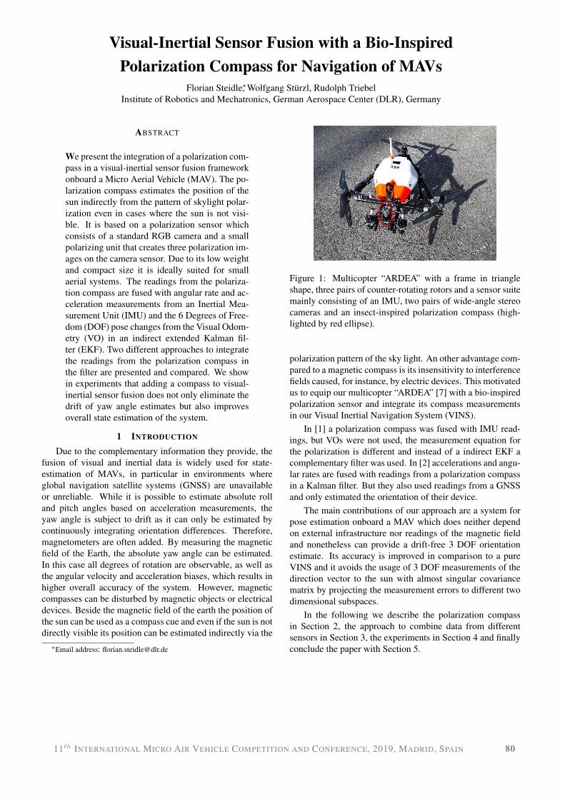
4.1 Test of the polarization compassAs an initial test, we placed the multicopter on a leveled

turntable and recorded the estimated sun azimuth and eleva-tion angles while turning the multicopter in steps of 30◦. Asillustrated in Figure 5, the sun position can be determinedquite accurately with a standard deviation below 1◦ for az-imuth and below 3◦ for elevation angle.

4.2 Indoor test of pose estimation with simulated measure-ments from the polarization compass

In the second experiment a trajectory of an indoor experi-ment in the lab was augmented with simulated measurementsof the polarization compass. The measurements of the po-larization compass were artificially corrupted by zero mean,white Gaussian noise. The noise levels were empirically de-termined. For the indoor datasets at each time stamp theground truth pose of ARDEA is available with high precision.


1 2 3 4 5 6 7 8 9 10 11 12 13

−180

−150

−120

−90

−60

−30

0

30

60

90

120

150

180

frame number

angle

[degre

e]

azimuth angle

elevation angle

Figure 5: Test of the sun position estimation by turning themulticopter in 30◦ steps. Shown are the azimuth angle withrespect to the initial orientation (green ’x’) and the sun eleva-tion angles (red ’x’) as estimated by the polarization compass.The dashed line shows the true sun elevation angle (≈ 32◦).

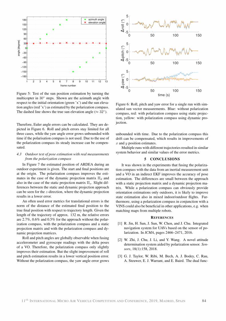
Therefore, Euler angle errors can be calculated. They are de-picted in Figure 6. Roll and pitch errors stay limited for allthree cases, while the yaw angle error grows unbounded withtime if the polarisation compass is not used. Due to the use ofthe polarization compass its steady increase can be compen-sated.

4.3 Outdoor test of pose estimation with real measurementsfrom the polarization compass

In Figure 7 the estimated position of ARDEA during anoutdoor experiment is given. The start and final positions areat the origin. The polarization compass improves the esti-mates in the case of the dynamic projection matrix Πd andalso in the case of the static projection matrix Πs. Slight dif-ferences between the static and dynamic projection approachcan be seen for the z-direction, where the dynamic projectionresults in a lower error.

An often used error metrics for translational errors is thenorm of the distance of the estimated final position to thetrue final position with respect to trajectory length. Given thelength of the trajectory of approx. 132 m, the relative errorsare 2.7%, 0.6% and 0.5% for the approach without the polar-ization compass, with the polarization compass and a staticprojection matrix and with the polarization compass and dy-namic projection matrices.

Roll and pitch angles are globally observable when fusingaccelerometer and gyroscope readings with the delta posesof a VO. Therefore, the polarization compass only slightlyimproves their estimation. But the slight improvement of rolland pitch estimation results in a lower vertical position error.Without the polarization compass, the yaw angle error grows

0 50 100 150-5

0

5

roll

(°)

0 50 100 150-5

0

5

pitch

(°)

0 50 100 150

time (s)

-5

0

5

ya

w (

°)Δ

ΔΔ

Figure 6: Roll, pitch and yaw error for a single run with sim-ulated sun vector measurements. Blue: without polarizationcompass, red: with polarization compass using static projec-tion, yellow: with polarization compass using dynamic pro-jection.

unbounded with time. Due to the polarization compass thisdrift can be compensated, which results in improvements ofx and y position estimates.

Multiple runs with different trajectories resulted in similarsystem behavior and similar values of the error metrics.

5 CONCLUSIONSIt was shown in the experiments that fusing the polariza-

tion compass with the data from an inertial measurement unitand a VO in an indirect EKF improves the accuracy of poseestimation. The differences are small between the approachwith a static projection matrix and a dynamic projection ma-trix. While a polarization compass can obviously provideorientation estimations only outdoors, it is likely to improvestate estimation also in mixed indoor/outdoor flights. Fur-thermore, using a polarization compass in conjunction with aVINS could also be beneficial in other applications, e.g. whenmatching maps from multiple robots.

REFERENCES

[1] R. Jin, H. Sun, J. Sun, W. Chen, and J. Chu. Integratednavigation system for UAVs based on the sensor of po-larization. In ICMA, pages 2466–2471, 2016.

[2] W. Zhi, J. Chu, J. Li, and Y. Wang. A novel attitudedetermination system aided by polarization sensor. Sen-sors, 18(1):158, 2018.

[3] G. J. Taylor, W. Ribi, M. Bech, A. J. Bodey, C. Rau,A. Steuwer, E. J. Warrant, and E. Baird. The dual func-


0 50 100 150

-15-10

5 0

x (

m) no pol. compass

static projection

dynamic projection

0 50 100 150

0

20

3 y(m

)

0 50 100 150

time (s)

00.5

1

z (

m)

Figure 7: Estimated position of ARDEA during an outdoorexperiment with and without the polarization compass.

tion of orchid bee ocelli as revealed by x-ray microto-mography. Current Biology, 26(10):1319–1324, 2016.

[4] W. Sturzl. A lightweight single-camera polarizationcompass with covariance estimation. In ICCV, pages5363–5371, 2017.

[5] G. Horvath and D. Varju. Polarized Light in AnimalVision: Polarization Patterns in Nature. Springer, 2004.

[6] R. Wehner and M. Mueller. The significance of di-rect sunlight and polarized skylight in the ant’s celes-tial system of navigation. Proceedings of the NationalAcademy of Sciences of the United States of America,103:12575–12579, 2006.

[7] M. G. Muller, F. Steidle, M. Schuster, P. Lutz, M. Maier,S. Stoneman, T. Tomic, and W. Sturzl. Robust visual-inertial state estimation with multiple odometries andefficient mapping on an MAV with ultra-wide FOVstereo vision. In IROS, 2018.

[8] D. Lambrinos, R. Moller, T. Labhart, R. Pfeifer, andR. Wehner. A mobile robot employing insect strate-gies for navigation. Robotics and Autonomous Systems,30:39–64, 2000.

[9] J. Chahl and A. Mizutani. Biomimetic attitude and ori-entation sensors. IEEE Sensors Journal, 12:289–297,2012.

[10] K. H. Strobl, W. Sepp, S. Fuchs, C. Paredes,M. Smisek, and K. Arbter. DLR CalDe and CalLab,www.robotic.dlr.de/callab/. Institute ofRobotics and Mechatronics, German Aerospace Center(DLR).

[11] W. J. MacLean. Removal of translation bias when usingsubspace methods. In ICCV, pages 753–758, 1999.

[12] K. Schmid, F. Ruess, M. Suppa, and D. Burschka. Stateestimation for highly dynamic flying systems using keyframe odometry with varying time delays. In IROS,pages 2997–3004, 2012.

[13] K. Schmid, F. Ruess, and D. Burschka. Local referencefilter for life-long vision aided inertial navigation. InFusion, 2014.

[14] N. Trawny and S. Roumeliotis. Sun sensor model. Uni-versity of Minnesota, Dept. of Comp. Sci. & Eng., Tech.Rep, 1, 2005.

[15] W. Forstner. Minimal representations for uncertaintyand estimation in projective spaces. In ACCV, pages619–632, 2010.


visual-inertial sensor fusion with a bio-inspired ... · south (seep-frame in figure 4). the exact...

Documents