visual inspection of hydroelectric dams using an …eia.udg.edu/~rafa/papers/jfr2010b.pdf · ·...

Visual Inspection of Hydroelectric Dams Usingan Autonomous Underwater Vehicle

• • • • • • • • • • • • • • • • • • • • • • • • • • • • • • • • • • • •

Pere Ridao, Marc Carreras, David Ribas, and Rafael GarciaComputer Vision and Robotics Research Group, Institute of Informatics and Applications, Universitat de Girona,Campus de Montilivi, 17071 Girona, Spaine-mail: [email protected], [email protected], [email protected], [email protected]

Received 15 January 2010; accepted 30 May 2010

This paper presents an automated solution to the visual inspection problem of hydroelectric dams. A small au-tonomous underwater vehicle, controllable in four degrees of freedom (surge, sway, heave, and yaw), is usedfor autonomously exploring the wall of a dam. The robot is easily programmed using a mission control lan-guage. Missions are executed by an intelligent control architecture that guides the robot to follow a predefinedpath surveying the wall. During the mission, the robot gathers onboard navigation data synchronized with op-tical imagery, sonar, and absolute navigation data, obtained from a moored buoy equipped with an ultra-shortbaseline system. After the mission, the images of the wall are used to build a photomosaic of the inspected area.First, image features are matched over the image sequence. Then, navigation data and interimage correspon-dences are optimized together using bundle adjustment techniques. Thus, a georeferenced globally aligned setof images is obtained. Finally, a blending algorithm is used to obtain smooth seam transitions among the dif-ferent images that constitute the mosaic, compensating for light artifacts and improving the visual perceptionof the scene. C© 2010 Wiley Periodicals, Inc.

1. INTRODUCTION

During the past two decades we have witnessed the appli-cation of autonomous underwater vehicles (AUVs) to tra-ditional fields such as marine science (German, Yoerger,Jakuba, Shank, Langmuir, et al., 2008), wreck (Eustice,Singh, Leonard, Walter, & Ballard, 2005) and underwater(Mindell & Bingham, 2001) archaeology, and maritime se-curity and energy sources (Hagen, Storkersen, & Vestgard,1999). Recently, the maturity of the technology, the cost re-duction of the underwater instrumentation, and the lat-est developments in underwater image processing haveopened the door to new applications of scientific (Pizarro &Singh, 2003; Pizarro, Eustice, & Singh, 2004; Singh, Roman,Pizarro, Eustice, & Can, 2007; Williams & Mahon, 2004), in-dustrial, and security (Negahdaripour & Firoozfam, 2006)interest. This article focuses on one of these applications:hydroelectric dam inspection. A preliminary meeting ofour research team with civil engineers from a Spanishpower generation company allowed us to identify the fol-lowing tasks of interest:

• Visual survey of the wall: assess the state of the concretefor safety purposes.

• Visual survey of the protecting fence of the water inletto the penstock gallery: assess the quantity of vegetalresiduals obstructing the water flow and reducing thegenerated power (see Figure 1).

A multimedia file may be found in the online version of this article.

Currently, these inspections are performed through a care-ful visualization of a video recorded by a professional diver,often without any localization information. Sometimes aglobal positioning system (GPS) reading gathered at thesurface is overlaid on the image, introducing an approxi-mate location of the underwater camera. A diver-trackingsystem may also be used, but even in this case the system isnot accurate enough to stitch all the images together to setup a global map of the surveyed area.

During the past several years, several companies haveclaimed to provide underwater robots for dam inspection(Seabotix, Inc., 2010; VideoRay LLC, 2010). Normally theypropose the use of small-class, remotely operated vehicles(ROV), working as teleoperated cameras for video record-ing, to replace the professional diver who traditionallyoccupied this place. Few research precedents provide anadded-value solution. One of the most relevant works isthe ROV3 system developed by the researchers of the In-stitut de Recherche HydroQuebec (Cote & Lavallee, 1995).This is a small ROV, localized through a long base line (LBL)system, which makes use of a multibeam sonar for collisionavoidance. The system is able to control the distance to thewall and includes several video cameras as well as a lasersystem for two-dimensional (2D) and three-dimensional(3D) measurements. The COMEX and Electricite de Francecompanies developed a similar project (Poupart, Benefice,& Plutarque, 2001). In this case, an ROV manufactured byCOMEX was localized using five LBL transponders. Again,several video cameras together with a 2D (double-spot)

Journal of Field Robotics 27(6), 759–778 (2010) C© 2010 Wiley Periodicals, Inc.View this article online at wileyonlinelibrary.com • DOI: 10.1002/rob.20351

760 • Journal of Field Robotics—2010

Figure 1. Vegetal residuals accumulated in the protecting fence of the water intake obstruct the inlet to the penstock pipe. Al-though this fence is commonly submerged, an unusually low level of the waterline made it visible in this picture.

laser system was used to take measurements. During 2002,in collaboration with the Research Development and Tech-nological Transfer Centre (CIFATT) IPA-Cluj, our team usedthe URIS robot working as an ROV to build an image mo-saic (Batlle, Nicosevici, Garcıa, & Carreras, 2003) of a smallarea of the wall of the Tartina Dam in the surroundingsof Cluj, Romania. To the best of the authors’ knowledge,this is the first time that image mosaicking techniques wereapplied for dam inspection. This solution gives an impor-tant added value because it provides civil engineers with aglobal view of the inspected area. Unfortunately, the ROVwas not localized, and hence the resulting image mosaicwas not georeferenced. The lack of this information makesit more difficult to perform periodic inspections on dam-aged spots and also to localize the areas where repair workmust take place.

Although very few works in dam inspection have beenreported in the literature, related work is available for in-specting the submerged portions of ship hulls, which is asimilar problem, especially when mapping the side hull. Inthis context, most of the recent work uses acoustic imagingsystems (Djapic, 2009; Englot & Hover, 2009), whose prin-cipal disadvantage is the cost of acoustic cameras, which isabout one order of magnitude greater than that of standardvision-based systems. A few authors have reported the useof systems based on optical cameras. In Negahdaripour andFiroozfam (2006), a stereo-vision system was used for robotpositioning, navigation, and mapping of the hull usingstereo images. This approach did not enable autonomousoperation but allowed the authors to achieve real-time ori-entation of an ROV with respect to the hull using uniquelystereo data, without any additional sensor. Kim and Eustice(2009) recently presented a calibrated monocular camerasystem mounted on a tilt actuator to keep a nadir view tothe hull. In this work, the authors used a pose-graph simul-taneous localization and mapping (SLAM) algorithm withan extended information filter for inference. A characteris-

tic of these works is that the proposed methods focus solelyon the construction of local maps and, hence, georeferenc-ing is not effectuated. This makes sense for ships and othermobile structures whose position is not fixed. However, asmentioned before, tasks such as dam inspection will ben-efit from this information during posterior surveillance ormaintenance tasks. In a related line of work, imaging sys-tems have also been used for the inspection of underwaterpipelines used in the telecommunication and oil industries(Antich, Ortiz, & Oliver, 2005; Balasuriya & Ura, 2002; Petil-lot, Reed, & Bell, 2002). However, most of the works focuson the detection and tracking of pipes rather than on thecreation of visual maps.

This article proposes the use of a highly maneuver-able AUV for automatically surveying a dam’s wall whilesnapping pictures and gathering navigation data in orderto build a globally optimized and georeferenced photomo-saic to enable systematic inspections. The robot can be pro-grammed using a mission control language (MCL). Mis-sions are executed by the intelligent control architecture ofthe robot, allowing the vehicle to follow a predefined pathwhile ensuring the vehicle safety. Navigation is achieved bycombining dead-reckoning data from the onboard sensors,a Doppler velocity log (DVL), and a motion reference unit(MRU) assisted by a fiber-optic gyro (FOG), with the cor-rections from a moored buoy equipped with an ultra-shortbaseline (USBL) compensated by a differential GPS (DGPS)and an MRU. A mechanical scanning imaging sonar is usedto detect and track the line feature corresponding to thedam’s wall. Combining the navigation data and the esti-mated line feature, is it possible to georeference the imagessnapped with the calibrated monocular vision system. Forthe problem at hand, and because a dam wall can be locallyapproximated by a planar surface with high accuracy, sim-ple methods for 2D photomosaicking can do the work, itnot being necessary to use more sophisticated methods for3D mapping as in Nicosevici, Gracias, Negahdaripour, and

Journal of Field Robotics DOI 10.1002/rob

Ridao et al.: Visual Inspection of Hydroelectric Dams Using an AUV • 761

Garcıa (2009), Pizarro et al. (2004), or Williams and Mahon(2004). Then, the visual information is merged with the nav-igation data to provide a globally registered photomosaic.At the end, a blending process is applied to smooth seamtransitions among the different images that constitute themosaic, compensating for light artifacts and improving thevisual perception of the scene.

The article is organized as follows. First, the experi-mental vehicle (Section 2) and its intelligent control archi-tecture (Section 3) are presented. Then, Sections 4 and 5introduce, respectively, the navigation system and the mod-ule used to detect and track the dam wall. Section 6 explainsthe method used to build the photomosaics, and the experi-mental results are reported in Section 7. Finally, conclusionsare presented in Section 8.

2. ICTINEU AUV

The research platform used in this project was composedof the Ictineu robot [see Figure 2(a)] and a surface buoy forglobally localizing the vehicle [see Figure 2(b)].

2.1. The Vehicle

The Ictineu vehicle (Ribas, Palomer, Ridao, Carreras, &Hernandez, 2007) was conceived around a typical openframe design [see Figure 2(a)] as a research prototypefor validating new technologies. It is a small (0.8 × 0.5 ×0.5 m), light (60 kg in air), and very-shallow-water (depthrating 30 m) vehicle. Although the hydrodynamics of open-frame vehicles is known to be less efficient than that ofclosed-hull-type vehicles, they are suitable for applicationsnot requiring movements at high velocities or travelinglong distances, such as a visual inspection of a dam. Thevehicle is practically neutral (approx. 0.6 kg of positive

buoyancy), it is stable in roll and pitch due to the weightand volume distribution, and it can be controlled in surge,sway, heave, and yaw with six Seabotix SBT150 thrusters.Each propeller can generate 22 N of force. Four of them areplaced horizontally in a rhombus configuration that makesit possible to thrust in any horizontal direction simultane-ously (surge and sway) and perform rotation (yaw). Theother two thrusters are placed vertically and can actuatethe heave degrees of freedom (DOF). The four DOF allowthe scanning of the wall of the dam while maintaining thedistance and point of view of the camera while moving ver-tically and horizontally.

The vehicle has two big cylindrical pressure vesselsthat house the power and computer modules. The powermodule contains a pack of sealed lead acid batteries, whichsupplies 24 Ah at 24 V and can provide the Ictineu withmore than 1 h of running time. The computer module hastwo PCs, one for control (PC104 AMD GEODE-300MHz)and one for image and sonar processing (mini-ITX com-puter Via C3 1 GHz) connected through a 100-Mbps Eth-ernet switch. An interesting characteristic of this vehicle isthat it can operate either as an ROV (tethered mode) or asan AUV (untethered mode). An optional umbilical cablecan be connected to the two modules to supply power andEthernet communication to the vehicle. This mode of oper-ation is very useful not only to operate the Ictineu as a ROVbut also to monitor the software architecture while the vehi-cle is performing the dam inspection autonomously. Whenworking in full AUV mode, the umbilical cable is removedand the vehicle relies on batteries to power all the systemsand therefore has a limited running time but a longer rangeof operation. Communication can then be established us-ing an acoustic modem, which is integrated in the USBLsensor. The sensors onboard the Ictineu AUV are listed inTable I.

(b)(a)Figure 2. (a) AUV Ictineu in water. (b) Surface buoy for localizing the vehicle.



Table I. Ictineu AUV sensor suite.

Sensor Model Characteristics

MSIS Tritech Miniking Maximum range: 100 mHorizontal beam width: 3 degScan rate: 5–20 s/360-deg sectorFrequency 675 kHz

DVL Sontek Argonaut Accuracy: 0.2% of measured velocityFrequency: 1,500 kHz

MRU + FOG Tritech iGC/iFG Accuracy: better than 1 degVision system B&W camera 1/3-in. charge-coupled device

0.01 lux50 Hz625 lines

Halogen lightsEcho sounder Airmar Smart Sensor Frequency: 235 kHzUSBL Linkquest Tracklink 1500 HA Angular accuracy: 0.25 deg

Range accuracy: 0.5% slant rangeFrequency: 31–43.2 kHz

2.2. The Surface Buoy

The purpose of the buoy is to determine the absoluteposition in world coordinates of the USBL transpondermounted on the vehicle. This information is necessary forgeoreferencing the sensor data acquired with the vehicleas well as to reduce the drift that inherently affects thedead-reckoning navigation estimate. A USBL consists of atransceiver, which is usually placed on the surface, and atransponder mounted on the AUV. The device determinesthe position of the vehicle by calculating the range and an-gles obtained after the transmission and reply of an acousticpulse between the transceiver and the transponder.

This buoy system is composed of a Linkquest Track-link 1500 USBL transceiver operating at 31–43.3 kHz andits supporting sensors, a DGPS and an Xsens MTi MRU,whose objective is to correct for the position and attitudechanges of the transceiver during the vehicle position esti-mation process. The different components are attached toa 1.5-m-high aluminum structure [see Figure 2(b)], whichdepending on the mission needs can be mounted out-board of a small boat or attached to a mooring buoy, asin the case of the experiments presented in this paper (seeFigure 3). The data logging is performed on an externalcomputer connected to the sensors through RS232. To in-tegrate the sensor information acquired with the robot withthe position estimates from the USBL system, the datashould have a common time base. For this reason, the com-puters in charge of the data logging are synchronized priorto the beginning of the mission. No significant time drifthas been observed for the typical mission duration (half anhour for the reported results).

3. INTELLIGENT CONTROL ARCHITECTURE

The intelligent control architecture has the goal of fulfill-ing the mission that has been predefined by a user. Thearchitecture acts as an hybrid control architecture (Arkin,1998), combining the continuous-time control laws corre-sponding to vehicle behaviors with a discrete event sys-tem (DES) responsible for enabling and disabling these be-haviors according to a particular mission plan. The hybridcontrol architecture is divided at the same time into twomain blocks: the software control architecture (SCA) and amission control system (MCS) (see Figure 4). The SCA con-tains the vehicle behaviors but also other systems or mod-ules. A perception module computes the state of the vehi-cle, and it obtains and processes sensor information fromthe robot interface module and sends the data to the con-trol module, which finally sets an output on the vehicle’sactuators. As can be seen in Figure 4, the control moduleis composed of a set of behaviors, a coordinator, and a ve-locity controller. The MCS is responsible for enabling anddisabling these behaviors. A Petri net formalism has beenchosen as the DES representation to model, program, andexecute AUV missions. To simplify the description of Petrinet missions, a MCL has been proposed. The user programsthe mission with MCL, and the MCL compiler transformsthis code into a Petri net (Palomeras, Ridao, Carreras, & Sil-vestre, 2009). Then, the real-time Petri net player executesthis Petri net mission by enabling/disabling the differentbehaviors of the SCA. An architecture abstraction layer(AAL) keeps the MCS independent from the vehicle SCA.The next subsections offer details about the SCA as well asthe MCS.



(b)(a)Figure 3. Images of the Ictineu vehicle and the surface buoy during the dam inspection experiments from the top of the dam(a) and from the shore (b).

3.1. Software Control Architecture

The vehicle architecture has to guarantee the AUV func-tionality. From the implementation point of view, the real-

time POSIX interface, together with the CORBA-RT (Tao,2003), has been used to develop the architecture as a setof distributed objects with soft real-time capabilities. The

MissionControl System

Software Control Architecture

Figure 4. Schematic of the intelligent control architecture used on Ictineu.



architecture is composed of a base system and a set of ob-jects customized for the desired robot. Software objects in-cluded in the architecture provide soft real-time capabili-ties, guaranteeing the execution period of tasks such as thecontrollers or the sensors. Another important part of thebase system is the loggers. A logger object is used to logdata from sensors, actuators, or any other object compo-nent. Moreover, all the computers in the network are syn-chronized so that all the data coming from different sensorscan be time related. The SCA is divided into three mod-ules: robot interface module, perception module, and con-trol module.

Robot Interface Module

The robot interface module contains software objects thatinteract with the hardware. Sensor objects are responsiblefor reading data from sensors, and actuator objects are re-sponsible for sending commands to the actuators. Sensorobjects include drivers for the surface buoy, MRU–FOG,DVL, imaging sonar, echo sounder, and camera. There arealso objects for the internal sensors, such as the water leak-age detectors and internal temperature and pressure sen-sors that allow for the monitoring of the conditions withinthe pressure vessels. For the output, one actuator objecthas been designed for every thruster. A virtual version ofevery component allows us to transparently connect therobot control architecture to a real-time graphical simulatorallowing hardware-in-the-loop simulations (Ridao, Batlle,Ribas, & Carreras, 2004).

Perception Module

This module contains two components: the navigator andthe environment detector. The navigator object has thegoal of estimating the position and velocity of the robot(Section 4), combining the data obtained by all the naviga-tion sensors. The control module uses the navigation dataprovided by the navigator, keeping the behaviors indepen-dent of the physical sensors being used for the localization.In the context of this application, the environment detectoris used to detect the relative position (range and bearing)of the dam’s wall with respect to the robot, as explained inSection 5.

Control Module

The control module acts as the reactive layer of our hy-brid control architecture. It receives sensor inputs fromthe perception module, keeping the behaviors indepen-dent of the physical sensors being used, and sends com-mand outputs to the actuators residing in the robot inter-face module. Several behaviors are defined to perform the

desired mission. Behaviors can be enabled and disabledand their parameters can be changed by means of actionssent by the MCS through the AAL. Also, events can be pro-duced by the behaviors to announce that a goal has beenreached or a failure has been detected within the vehiclearchitecture.

In particular, the following behaviors were developedto perform the inspection of the dam:

• GoTo: Performs a trajectory from the current position tothe specified X, Y , and Z positions and yaw orientation.Takes the position and orientation data from the naviga-tor object.

• WallInspection: Used to follow a 2D path in Y and Z

DOF in front of the wall of the dam following a sequenceof waypoints (path).

• AchieveHeadDist: Allows the robot to keep a prepro-grammed distance and heading with respect to the wall,which are estimated by the environment detector object.

• Surface: Performs a vertical trajectory from the currentposition to the surface.

• StartCamera: Sensing behavior used to enable/disablethe vehicle frontal camera to gather images of the wall.

• Alarms: Sensing behavior responsible for issuing anevent if water leakage or a dangerous temperature orpressure is detected inside a pressure vessel.

3.2. Mission Control System

The MCS acts as a deliberative and control execution layerof our hybrid control architecture. However, the MCS doesnot automatically plan the set of active behaviors at eachmoment. A user describes the mission using a high-levellanguage called MCL, and then the mission is automaticallytranslated into a DES represented as a Petri net that is ableto decide which behaviors will be executed depending onthe observed events.

The MCS has been designed to be as generic as pos-sible. To achieve this goal, the proposed MCS presents aclear interface with any particular vehicle control architec-ture based on actions and events. Actions are specific or-ders given by the MCS to the control architecture to en-able one behavior or to configure parameters. Events aresome facts that the control architecture detects or mea-sures, which are sent to the MCS. Between the MCS andthe vehicle control architecture, there is an AAL that adaptsthese actions and events for every particular architecture(see Figure 4). The AAL depends on the control archi-tecture being used, allowing the MCS to remain architec-ture independent. With the AAL, it is possible to use thisMCS approach in different vehicles with different controlarchitectures.

A mission is programmed using a set of parallel execu-tion flows, each one involving an iterative/sequential exe-cution of tasks. In our system, a task is the basic execution



block at the event-driven domain. When a task begins, it en-ables (by means of actions sent through the AAL) the set ofbehaviors (running in the time domain) needed to achieveits associated goals. When certain conditions are detected(by means of events or timeouts), the task disables the set ofbehaviors. Tasks have two possible ending status, correct orfail. Internally, tasks are modeled using the Petri net formal-ism (Murata, 1989) and can be joined using control struc-tures (if-then-else, try-catch...) to set up mission programs.The control structures themselves are encoded using Petrinets, and so it is the full mission program. The adoptionof the Petri net formalism allows us to do formal verifica-tions such as asserting deadlock avoidance and ensuringthe mission progress from the initial state to one of the pos-sible ending estates. To avoid the burden of programmingthe mission directly as a Petri net, a MCL has been de-fined (Palomeras, Ridao, Carreras, & Silvestre, 2008). MCLmission programs are automatically translated into a Petrinet representing the mission. A complete description of ourMCS and MCL can be found in Palomeras et al. (2008) andPalomeras et al. (2009), respectively.

The following structures are supported by the MCLlanguage:

Sequence: Used to execute one block of tasks after an-other. In an MCL code (an example can beseen in Algorithm 1), the sequence com-mand is represented with a semicolon. It isworth noting that the last task in a blockfinishes without semicolon.

Try-Catch-Do: Executes the try block in parallel with thecatch block. If the former finishes before thelatter, the catch block is canceled and theexecution continues after the try-catch-dostructure. However, if the catch block fin-ishes first, the try block is aborted and thedo block is executed.

Parallel-And: Executes two blocks in parallel. If bothblocks finish correctly, the whole controlstructure finishes correctly. Otherwise, theparallel-and finishes with a fail status.

Parallel-Or: Executes two blocks in parallel. The firststructure to finish aborts the other. Theparallel-or finishes with the final state ofthe first block to end.

If-Then-Else: Executes the block inside the if statementand, depending on whether the block endswith an ok or fail, the block inside the thenstatement or the else statement is executed,respectively.

While-do: Executes the block inside the while state-ment. If this block finishes with an ok,it executes the do statement; otherwise itends with an ok. If the do statement fin-ishes with an ok, it executes again the while

statement; otherwise the whole structureends with a fail.

The control structures together with the tasks constitute theMCL code that will be finally compiled to create the Petrinet that represents the mission.

For the mission presented in this paper, the tasks thatwere needed are as follows:

• Alarms() Checks the events related with the alarms be-havior.

• StartLogs() Starts or stops all the log objects to save thedata.

• GoTo() Sets the goal position of the GoTo behavior andwaits until the position is achieved.

• AchieveHeadDist() Sets the parameters of the Achieve-HeadDist behavior and waits until the heading and dis-tance are achieved.

• KeepHeadDist() Sets the parameters of the Achieve-HeadDist behavior and starts or stops it.

• KeepHeadDistException() Evaluates whether the head-ing and distance cannot be achieved by checking its cor-responding event.

• StartCamera() Starts or stops the camera acquisition.• WallInspect() Sets the parameters of the WallInspection

behavior and waits until the trajectory is achieved.• Surface() Starts the Surface behavior and waits until it

finishes.

Using these tasks, the dam inspection mission is describedas follows. After checking all the alarms, the sensor logsare enabled and, in parallel with the rest of the mission,two monitors are used to send an event in case the pres-sure/temperature exceeds a threshold or if a water leakageis detected inside a pressure vessel. Using the GoTo behav-ior, the vehicle goes to the initial waypoint of the surveyand, after achieving the desired orientation and distancewith respect to the dam wall, the survey starts. Duringthe survey, imagery is recorded using the black-and-whitecamera looking forward. When the survey finalizes, thecamera stops, the vehicle goes to the recovery position, andthe logs are disabled. If during the mission any of the mon-itors generates an alarm event, the mission is aborted andthe vehicle surfaces.

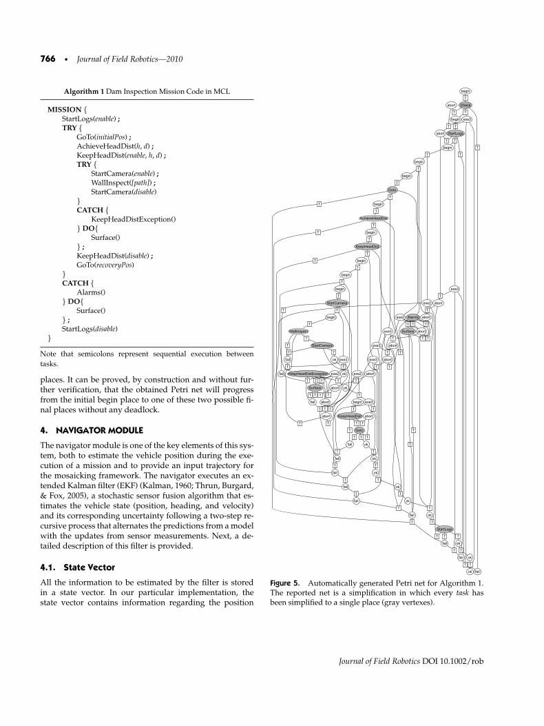
The mission program (see Algorithm 1) was pro-grammed and compiled into a Petri net representing themission (Palomeras et al., 2008). The try-catch-do controlstructure was used to describe all possibilities and to exe-cute the blocks of actions accordingly. Figure 5 shows a sim-plified version of the resulting Petri net. In the figure, taskshave been simplified to single places (gray vertexes) andtransitions are shown as squares with a T inside. The placeslabeled as begin, abort, ok, and fail are used to start, stop,and indicate the finalization state of each task. The Petrinet starts with begin/abort places and finalizes with ok/fail



Algorithm 1 Dam Inspection Mission Code in MCL

MISSION {StartLogs(enable) ;TRY {

GoTo(initialPos) ;AchieveHeadDist(h, d) ;KeepHeadDist(enable, h, d) ;TRY {

StartCamera(enable) ;WallInspect([path]) ;StartCamera(disable)

}CATCH {

KeepHeadDistException()} DO{

Surface()} ;KeepHeadDist(disable) ;GoTo(recoveryPos)

}CATCH {

Alarms()} DO{

Surface()} ;StartLogs(disable)

}

Note that semicolons represent sequential execution betweentasks.

places. It can be proved, by construction and without fur-ther verification, that the obtained Petri net will progressfrom the initial begin place to one of these two possible fi-nal places without any deadlock.

4. NAVIGATOR MODULE

The navigator module is one of the key elements of this sys-tem, both to estimate the vehicle position during the exe-cution of a mission and to provide an input trajectory forthe mosaicking framework. The navigator executes an ex-tended Kalman filter (EKF) (Kalman, 1960; Thrun, Burgard,& Fox, 2005), a stochastic sensor fusion algorithm that es-timates the vehicle state (position, heading, and velocity)and its corresponding uncertainty following a two-step re-cursive process that alternates the predictions from a modelwith the updates from sensor measurements. Next, a de-tailed description of this filter is provided.

4.1. State Vector

All the information to be estimated by the filter is storedin a state vector. In our particular implementation, thestate vector contains information regarding the position

Figure 5. Automatically generated Petri net for Algorithm 1.The reported net is a simplification in which every task hasbeen simplified to a single place (gray vertexes).



Figure 6. Reference frames involved in the proposed system.

and velocity of the vehicle at time k:

x(k) = [x y z ψ u v w r]T , (1)

where, following the nomenclature proposed in Fossen(1994), the vector [x y z ψ] represents the position and head-ing of the vehicle in the global reference {W } (see Figure 6)and [u v w r] are the linear and angular velocities, whichare represented on the vehicle’s coordinate frame {V }. Be-cause the Ictineu vehicle is passively stable in roll and pitch,their corresponding angles and velocities have not been in-cluded in the state vector.

4.2. Initializing the Filter

At the beginning of the mission and before starting theKalman filter, the initial value of the state vector x(0) shouldbe determined. With measurements from the surface buoyavailable, it is possible to determine the vehicle’s initial po-sition with respect to the global reference {W }. Therefore,the first measurement from the buoy system, and its asso-ciated uncertainty, will be used to define the initial positionof the vehicle. Because {W } is aligned with the north, thesame strategy can be used to initialize the heading with thecompass-referenced FOG. During the initialization phase,the vehicle is kept almost static. Therefore, it is not un-realistic to initialize the velocities with a zero mean butincluding some uncertainty to account for possible per-turbations. The resulting estimate for the state vector at

time 0 is

x(0) =

⎡⎢⎢⎢⎢⎢⎢⎢⎢⎢⎢⎣

xU

yU

zU

ψC

0000

⎤⎥⎥⎥⎥⎥⎥⎥⎥⎥⎥⎦

,

P(0) =

⎡⎢⎢⎢⎢⎢⎢⎢⎢⎢⎢⎢⎣

σ 2Ux σUxy σUxz 0 0 0 0 0

σUyx σ 2Uy σUyz 0 0 0 0 0

σUzx σUzy σ 2Uz 0 0 0 0 0

0 0 0 σ 2C 0 0 0 0

0 0 0 0 σ 2u 0 0 0

0 0 0 0 0 σ 2v 0 0

0 0 0 0 0 0 σ 2w 0

0 0 0 0 0 0 0 σ 2r

⎤⎥⎥⎥⎥⎥⎥⎥⎥⎥⎥⎥⎦

,

(2)

where the subindex U stands for the USBL and C for thecompass. Note that the position covariance submatrix isnot diagonal. The data from the buoy system are the re-sult of combining the information from the GPS and theMRU with the vehicle position measured from the USBLtransceiver; hence the estimated global position is corre-lated. These correlations can be determined by setting eachsensor’s covariance according to the manufacturer specifi-cations and then defining the necessary transformations toproduce the vehicle position in world coordinates; that is,combining a GPS reading with the angular measurementsfrom the MRU to obtain the position and attitude of thebuoy and then composing it with the USBL measurement



(in spherical coordinates) to produce the vehicle position inCartesian coordinates.

4.3. System Model

A simple four-DOF constant velocity kinematics model isused to predict how the state will evolve from time k − 1 totime k:

x(k) = f (x(k − 1), n(k − 1)),⎡⎢⎢⎢⎢⎢⎢⎢⎢⎢⎢⎣

x

y

z

ψ

u

v

w

r

⎤⎥⎥⎥⎥⎥⎥⎥⎥⎥⎥⎦

(k)

=

⎡⎢⎢⎢⎢⎢⎢⎢⎢⎢⎢⎢⎢⎢⎢⎢⎢⎢⎢⎢⎢⎢⎣

x +(

ut + nut2

2

)cos(ψ) −

(vt + nv

t2

2

)sin(ψ)

y +(

ut + nut2

2

)sin(ψ) +

(vt + nv

t2

2

)cos(ψ)

z + wt + nwt2

2

ψ + rt + nrt2

2u + nut

v + nvt

w + nwt

r + nr t

⎤⎥⎥⎥⎥⎥⎥⎥⎥⎥⎥⎥⎥⎥⎥⎥⎥⎥⎥⎥⎥⎥⎦

(k−1)

, (3)

where t is the time period and n = [nu nv nw nr ]T repre-sents a vector of white Gaussian acceleration noises withzero mean whose covariance values have been set empiri-cally according to the observed performance of the constantvelocity model. They are additive in the velocity terms andpropagate through integration to the position. The covari-ance of the n vector is represented by the system noise ma-trix Q:

E [n(k)] = 0, E[n(k)n(j )T ] = δkj Q(k), (4)

Q =

⎡⎢⎢⎣

σ 2nv

0 0 00 σ 2

nu0 0

0 0 σ 2nw

00 0 0 σ 2

nr

⎤⎥⎥⎦ . (5)

The model described in Eqs. (3) is nonlinear and thereforethe prediction should be performed with the EKF equations(Thrun et al., 2005).

4.4. Measurement Model

The vehicle is equipped with a number of sensors provid-ing direct observations of particular elements of the state

vector. The general linear model for such measurements iswritten in the form

z(k) = Hx(k|k − 1) + m(k),⎡⎢⎢⎢⎢⎢⎢⎢⎢⎢⎢⎣

zuD

zvD

zwD

zzP

zψC

zxU

zyU

zzU

⎤⎥⎥⎥⎥⎥⎥⎥⎥⎥⎥⎦

(k)

=

⎡⎢⎢⎢⎢⎢⎢⎢⎢⎢⎢⎣

0 0 0 0 1 0 0 00 0 0 0 0 1 0 00 0 0 0 0 0 1 00 0 1 0 0 0 0 00 0 0 1 0 0 0 01 0 0 0 0 0 0 00 1 0 0 0 0 0 00 0 1 0 0 0 0 0

⎤⎥⎥⎥⎥⎥⎥⎥⎥⎥⎥⎦

⎡⎢⎢⎢⎢⎢⎢⎢⎢⎢⎢⎣

x

y

z

ψ

u

v

w

r

⎤⎥⎥⎥⎥⎥⎥⎥⎥⎥⎥⎦

(k)

+

⎡⎢⎢⎢⎢⎢⎢⎢⎢⎢⎢⎣

muD

mvD

mwD

mzP

mψC

mxU

myU

mzU

⎤⎥⎥⎥⎥⎥⎥⎥⎥⎥⎥⎦

(k)

, (6)

where the subindex U stands for the USBL, C for the com-pass, D for the DVL, and P for the pressure sensor; z isthe measurement vector, and m represents a vector of whiteGaussian noises with zero mean, affecting the observationprocess. The covariance matrix of the measurement noise Ris given by

E[m(k)] = 0, E[m(k)m(j )T ] = δkj R(k), (7)

R(k) =

×

⎡⎢⎢⎢⎢⎢⎢⎢⎢⎢⎢⎢⎢⎣

σ 2Du σDuv σDuw 0 0 0 0 0

σDvu σ 2Dv σDvw 0 0 0 0 0

σDwu σDwv σ 2Dw 0 0 0 0 0

0 0 0 σ 2P

0 0 0 00 0 0 0 σ 2

ψ 0 0 00 0 0 0 0 σ 2

Ux σUxy σUxz

0 0 0 0 0 σUyx σ 2Uy σUyz

0 0 0 0 0 σUzx σUzy σ 2Uz

⎤⎥⎥⎥⎥⎥⎥⎥⎥⎥⎥⎥⎥⎦

(k)

.

(8)

The covariance values for the R matrix have been assignedaccording to the specifications from the manufacturers ofeach particular sensor. The form of the observation matrixH changes according to the measurements available fromthe sensors at each time step k.

Note that the DVL covariance submatrix is not diago-nal. The reason behind these correlations is that the mea-surements provided by the DVL are not directly observedbut are calculated from the projection of the vehicle’s ve-locity onto the multiple-beam axes of the sensor. The cor-relation of the measurements depends on the beam geom-etry and, hence, should be determined for each particulardevice (Brokloff, 1994). In our particular implementation,



these correlations have been determined for the three-beamconfiguration of our DVL (Ribas, Ridao, & Neira, 2010). Thesame happens for the USBL covariance submatrix, which isfull because the USBL fix is represented in Cartesian coor-dinates instead of cylindrical as usual.

4.5. Trajectory Smoothing

To produce a better trajectory estimate, the state vectorcan be augmented with a history of past vehicle positions(Leonard & Rikoski, 2001; Smith, Self, & Cheeseman, 1990).Executing an augmented state Kalman filter allows thepropagation of sensor information to past states throughtheir correlation with the current estimate. As a result ofthis process, their values are refined and a smooth esti-mated trajectory is obtained. To limit the computationalburden of a growing augmented state vector, it is possibleto remove the older clones from the state after some time.In an estimator such as the one proposed here, the most re-cent clones are the ones more strongly correlated with thecurrent vehicle state. Therefore, the information from a sen-sor measurement will propagate strongly to them but havealmost no effect to the older ones.

Performing this trajectory smoothing is not necessaryduring the mission. However, it has been employed dur-ing the offline postprocessing of navigation data to producea better trajectory estimate for the photomosaic-buildingframework.

5. WALL DETECTION AND TRACKING

This section presents the algorithm developed for theenvironment detector (see Section 3), a key element of thesystem whose function is to detect and track the dam wallduring the autonomous execution of the survey using themechanically scanned imaging sonar (MSIS) onboard thevehicle. The objective of this algorithm is to provide thenecessary information to ensure that the vehicle is facingthe dam wall perpendicularly and at a particular distanceto avoid distortions on the acquired images.

Although dam walls are generally curved to improvethe structural resistance to the water pressure, they can belocally approximated by a line feature (see Figure 7). Thesevertical and planar structures can be efficiently detected inacoustic images (Kazmi, Ridao, Ribas, & Hernandez, 2009).The process begins with the estimation of the initial posi-tion of the wall with respect to the vehicle. First, the imagegathered with the MSIS is binarized. After discarding theecho intensity readings in the neighborhood of the sonarhead, the highest-intensity echo return is located and usedto compute the range for each beam corresponding to aparticular bearing. A modified procedure is used to com-pute the Hough transform (HT) in which the set of admis-sible lines containing a point is restricted to those that alsosatisfy a tangency criterion resulting from the finite beamwidth of the sonar. Once the initial line candidate has been

computed, it is further refined through a tracking processinvolving a Kalman filter, in which the information fromthe heading sensor and the points extracted from the sonardata are used to update the line estimate and hence trackthe position of the dam wall with respect to the vehicle. It isworth mentioning that although this tracking filter could beeasily integrated into the navigation filter presented in thepreceding section, it has been implemented as an indepen-dent module to allow for alternative tracking methods inthose situations in which the planar wall assumption doesnot hold. Next, we describe the sonar model used for theHT voting.

5.1. Sonar Model

Owing to the horizontal beam width, a sonar readingcannot be related to a single point in space. In Leonardand Durrant-Whyte (1992), a sonar model is described inwhich a polar measurement [ρS θS ] is not associated witha unique point but with an arc of points placed at a rangeρS and within an aperture α being centered in the directionθS of the actual sonar measurement. Therefore the points[ρα,i θα,i ] associated with the measurement are those satis-fying

θS − α/2 ≤ θα,i ≤ θS + α/2; ρα,i = ρS, (9)

which extends the sonar measurement with a range of pos-sible bearings within the horizontal aperture α of the beam(where α = 3 deg in our case). Hence, the set of candi-date lines (corresponding to planar objects) that can ex-plain the sonar measurement are those tangent to the arc.Although this model is suitable for mobile robots usinglow-resolution, wide-angle sonar beams, it still needs to beimproved to explain the behavior experimentally observedwith the MSIS. As can be seen in Figure 7, the visibility ofthe dam wall is not limited to those objects tangent to thenarrow beam width of the sonar. In fact, high echo intensityvalues are clearly obtained 2–3 m around the nadir point. Itcan also be observed that although the wall is still visible atboth ends of the line, the intensity and the precision of themeasurement decreases. In Ribas, Neira, Ridao, and Tardos(2006), the previous sonar model was further extended forbeams with a narrow horizontal aperture and working un-derwater. In this case, the measurements are associated notonly to the arc tangent surfaces within the horizontal aper-ture but also to the surfaces incident at certain angles β

(for the MiniKing imaging sonar, we have observed that aβ = 60 deg works fine for most of the tested wall surfaces).Now, a line [ρβ,k, θβ,k] candidate to correspond with a sonarmeasurement is described by relation (10) and Eq. (11) (seeFigure 8):

θα,i − β ≤ θβ,k ≤ θα,i + β, (10)

ρβ,k = ρα,i cos(θα,i − θβ,k). (11)



Figure 7. 180-deg sonar scan sector of the dam’s wall.

5.2. Filter Initialization

As mentioned above, the HT is used to produce an initialestimate for the position of the dam wall given the measure-ments contained in the sonar scan. After selecting the binswith the highest echo return, the set of compatible line can-didates are determined according to the model describedin the preceding section. The voting process begins by ini-tializing a Hough space consisting of a discretized repre-sentation of a [ρ θ ] space in which all candidate lines arerepresented. Then, the subset of candidate lines that are

Figure 8. Modified sonar model.

compatible with a particular sonar measurement determinewhich cells of the Hough space should receive a vote. Theprocess of assigning votes is repeated for all the measure-ments contained in the scan. After the voting, the cell inthe Hough space with the largest number of votes is theone representing the line candidate that more likely corre-sponds with the real position of the wall. Therefore, thisline feature [VρL

VθL] is chosen to initialize the state vectorof the Kalman filter:

x(0) =⎡⎣VρL

VθLWθL

⎤⎦ , (12)

where the term WθL corresponds to the parameterizationof the line orientation with respect to the global frame {W }defined as (see Figure 9)

WθL = ψ + VθL. (13)

The uncertainty of this initial state is defined as

P(0) =

⎡⎢⎣

σ 2VρL

0 00 σ 2

VθLσVθL,WθL

0 σWθL,VθLσ 2

WθL

⎤⎥⎦ , (14)

where it has been assumed that the robot was static enoughduring the first scan to consider WθL independent from ψ ,so

σ 2WθL

= σ 2VθL

+ σ 2ψ ; σVθL,WθL

= σ 2VθL

. (15)

Although, as stated in Ribas, Ridao, Tardos, and Neira(2008), it is possible to obtain an estimate of the covariance



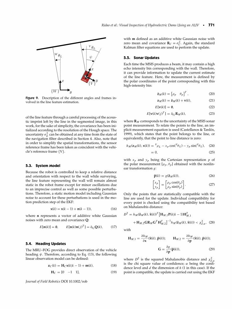
Figure 9. Description of the different angles and frames in-volved in the line feature estimation.

of the line feature through a careful processing of the acous-tic imprint left by the line in the segmented image, in thiswork, for the sake of simplicity, the covariance has been ini-tialized according to the resolution of the Hough space. Theuncertainty σ 2

ψ can be obtained at any time from the state ofthe navigation filter described in Section 4. Also, note thatin order to simplify the spatial transformations, the sensorreference frame has been taken as coincident with the vehi-cle’s reference frame {V}.

5.3. System Model

Because the robot is controlled to keep a relative distanceand orientation with respect to the wall while surveying,the line feature representing the wall will remain almoststatic in the robot frame except for minor oscillations dueto an imprecise control as well as some possible perturba-tions. Therefore, a static motion model including Gaussiannoise to account for these perturbations is used in the mo-tion prediction step of the EKF:

x(k) = x(k − 1) + n(k − 1)), (16)

where n represents a vector of additive white Gaussiannoises with zero mean and covariance Q:

E[n(k)] = 0, E[n(k)n(j )T ] = δkj Q(k), (17)

5.4. Heading Updates

The MRU–FOG provides direct observation of the vehicleheading ψ . Therefore, according to Eq. (13), the followinglinear observation model can be defined:

zC (k) = HCx(k|k − 1) + m(k), (18)

HC = [0 −1 1], (19)

with m defined as an additive white Gaussian noise withzero mean and covariance RC = σ 2

C . Again, the standardKalman filter equations are used to perform the update.

5.5. Sonar Updates

Each time the MSIS produces a beam, it may contain a highecho intensity bin corresponding with the wall. Therefore,it can provide information to update the current estimateof the line feature. Here, the measurement is defined bythe polar coordinates of the point corresponding with thishigh-intensity bin:

zM (k) = [ρp θp

]T, (20)

zM (k) = zM (k) + v(k), (21)

E[v(k)] = 0, (22)

E[v(k)v(j )T ] = δkj RM (k), (23)

where RM corresponds to the uncertainty of the MSIS sonarpoint measurement. To relate the points to the line, an im-plicit measurement equation is used (Castellanos & Tardos,1999), which states that the point belongs to the line, orequivalently, that the point to line distance is zero:

hM (zM (k), x(k)) = VρL − xp cos(VθL) − yp sin(VθL), (24)

= 0, (25)

with xp and yp being the Cartesian representation p ofthe polar measurement [ρp, θp] obtained with the nonlin-ear transformation g:

p(k) = g(zM (k)), (26)[xp

yp

]=

[ρp cos(θp)ρp sin(θp)

]. (27)

Only the points that are statistically compatible with theline are used for the update. Individual compatibility forevery point is checked using the compatibility test basedon Mahalanobis distance:

D2 = hM (zM (k), x(k))T[HM,1P(k|k − 1)HT

M,1

+ HM,2GRMGT HTM,2

]−1hM (zM (k), x(k)) < χ2

d,α, (28)

with

HM,1 = ∂hM

∂x(x(k), p(k)); HM,2 = ∂hM

∂p(x(k), p(k));

G = ∂g

∂p(p(k)), (29)

where D2 is the squared Mahalanobis distance and χ2d,α

is the chi square value of confidence; α being the confi-dence level and d the dimension of h (1 in this case). If thepoint is compatible, the update is carried out using the EKF



equations for an implicit measurement function:

K(k) = P(k|k − 1)HTM,1

[HM,1P(k|k − 1)HT

M,1

+ HM,2GRMGT HTM,2

]−1, (30)

x(k) = x(k|k − 1) − K(k)hM (zM (k), x(k)), (31)

P(k) = [I − K(k)HM,1]P(k|k − 1). (32)

6. BUILDING PHOTOMOSAICS OF THE DAM

6.1. Camera Modeling

To carry out precise and reliable measurements from im-ages, camera calibration is a necessary prerequisite. Imagesare first corrected for lens distortion, and the camera ismodeled as the classical projective pinhole camera (Hart-ley & Zisserman, 2004) using Bouget’s toolbox (Bouguet,2010), which defines the projection of the 3D point WXj inthe world onto the image plane {i} as

ixj = K · CWR · [I WT] · WXj , (33)

where K encodes the intrinsic camera parameters and CWR is

the 3 × 3 rotation matrix that transforms vector coordinatesdefined in the world coordinate frame {W } to coordinatesin the camera frame {C}; WT is the translation of the cameracenter with respect to the frame {W }, and ixj is the j th 2Dpoint in homogeneous coordinates that corresponds to theprojection onto the image plane of the scene 3D point WXj .

6.2. Robust Matching

A crucial part in the mosaicking workflow is the registra-tion (or matching) of two or more images of the same scenetaken at different times and from different viewpoints. Forthis reason, special effort is devoted in this work to ensurerobust image registration through a three-step mechanism.

First, SURF (Bay, Tuytelaars, & Gool, 2006) features areextracted from both images. Then, a putative set of corre-spondences is obtained (Bay et al., 2006), and outliers arerejected using RANSAC (Fischler & Bolles, 1981) under aplanar projective motion model (using a homography witheight DOF) (Brown & Lowe, 2003; Vincent & Laganiere,2001). The remaining inliers are then used to compute thehomography that registers both images (Hartley & Zisser-man, 2004). As a third step, a number of verifications areperformed to ensure that this homography corresponds toa valid camera motion:

1. The obtained homography does not include improperrotations.

2. The 3D motion Euler angles associated to this planartransformation are within a certain range (Triggs, 1998).

3. The number of SURF correspondences between the twoimages must be larger than a certain threshold.

4. The overlapping area between the images must behigher than a threshold.

As a last step, further point correspondences are searchedfor in the image pairs that passed successfully the abovetests. The two images are aligned according to the pre-viously estimated homography. Then, we extract Harriscorners (Harris & Stephens, 1988) in one of the images,and their correspondences are detected through correlation(Garcia, Batlle, Cufı, & Amat, 2001) in the other image. Ifenough correspondences are not found, the pair of imagesis rejected.

The process described above is used first to obtaincorrespondences between time-consecutive images. We as-sume that each pair of consecutive images of the sequenceis a potential candidate to be a sequential pair of overlap-ping frames (although they may not overlap in some cases).

The matching process is run offline on a dedicatedserver that requires slightly more than a second to processevery image.

6.3. Navigation Data

Although image processing produces locally coherent im-age alignment, it requires position estimates from vehi-cle navigation to avoid significant drifts in the localiza-tion of images because of the cumulative error of succes-sive matchings. The available sensor suite (USBL, DGPS,MRU in the moored buoy, and the DVL and MRU–FOG inthe vehicle) provides navigation data corresponding to theposition and the heading of the vehicle with respect to theworld coordinate frame {W }. Therefore, this information isalso taken into account to build the photomosaic, by regis-tering the mosaic in the world frame.

6.4. Loop Detection and Registrationof Nonconsecutive Images

To obtain a globally coherent mosaic, the next step is thedetection of nonconsecutive overlapping pairs of images.When the vehicle revisits a previously mapped area, newconstraints for the global alignment of the photomosaicare provided. Possible crossings are identified using mo-tion estimation from consecutive images and from vehi-cle navigation data. Therefore, a method to include all thepossible overlaps has been devised. The center of eachimage is computed offline in the 2D mosaic frame ac-cording to the planar transformations obtained from theregistration of consecutive images and the previously es-timated navigation data. These two data sources (imagecues and navigation data) are merged through a nonlin-ear optimization (bundle adjustment) that minimizes thecost function described in the next section. A set of imagesthat are mapped closer than a certain threshold from thecrossover point are analyzed to identify candidate imagepairs that are then robustly matched using the proceduredescribed in Section 6.2. The pairs retained with the associ-ated correspondence points are used as input for the globalalignment.



6.5. Global Alignment

Although our vehicle is roll and pitch stable, to keep theimage processing system generic enough to be applied toother vehicles, we parameterize the camera trajectory in themost general terms with six DOF (3D position and orienta-tion) using unitary quaternions (Salamin, 1979) to preventsingularities in the representation of the camera rotation.Therefore, pose rotation matrices are converted into unitquaternions C

Mqj. This gives three parameters for the po-

sition and four for the orientation, giving rise to seven pa-rameters to be estimated for each image frame j .

An offline bundle adjustment (Triggs, McLauchlan,Hartley, & Fitzgibbon, 2000) procedure is used to minimizethe residuals from image registration and estimated navi-gation data (see Section 4).

The cost function to perform global alignment is de-fined as the weighted sum of three terms: (1) the squaredresidual of the robot position, (2) the squared residual ofthe robot attitude, and (3) the squared residual of the pointmatchings in the image plane. The position and attituderesiduals are computed from the navigation data. Given acertain point feature p, observed as p1 and p2 in the im-age planes corresponding to two different views I1 and I2,respectively, the point matching residual is computed asthe difference between p1 and the reprojection of p2 intothe image plane corresponding to I1. The minimization ofthe cost function and the estimation of the trajectory pa-rameters are carried out using Matlab’s large-scale meth-ods for nonlinear least squares (Escartın, Garcia, Delaunoy,Ferrer, Gracias, et al., 2008). The optimization algorithm re-quires the computation of the Jacobian matrix containingthe derivatives of all residuals with respect to all trajectoryparameters. Fortunately, this Jacobian matrix is very sparsebecause each residual depends on only a very small num-ber of parameters (Triggs et al., 2000). Furthermore, it has aclearly defined block structure, and the sparsity pattern isconstant (Capel, 2004). These conditions allow for the effi-cient computation of the Jacobian. In our implementation,analytic expressions were derived and used for computingthe blocks of the Jacobian matrix.

6.6. Loop Detection and Optimization Iteration

Mosaic alignment is improved through several iterations ofloop detection and optimization. After each iteration, theresulting optimized trajectory of the camera is used as astarting point for a new iteration of detection of new poten-tial overlapping image pairs and bundle adjustment to findnew constraints (i.e., more overlapping image pairs nearcrossings). Iterations are repeated until no new crossoversare detected. The number of iterations depends on the qual-ity of the data, but normally three to four iterations isenough.

6.7. Blending of the Photomosaic

The globally aligned mosaic must be blended to compen-sate for nonuniform illumination, caustics (from reflectionswhen close to the surface), blurring, and suspended par-ticles and scattering, especially in turbid waters, which isthe case in most lakes and dams. For this reason, we ren-der the optimized mosaic by projecting every individualimage onto the mosaic plane. The rendering of every pixelis decided as a function that penalizes the distance fromthat pixel to the center of the image, because central pix-els are normally better exposed than those on the borderof the image. Finally, this composite mosaic is transferredto the gradient domain, where we compensate for the gra-dients at the image seams, and a least-squares solution isfound by solving a discrete Poisson equation, going backto the spatial domain to obtain the seamless blended mo-saic. More details about an algorithm specifically adaptedto blend large mosaics can be found in Prados (2007).

7. EXPERIMENTS

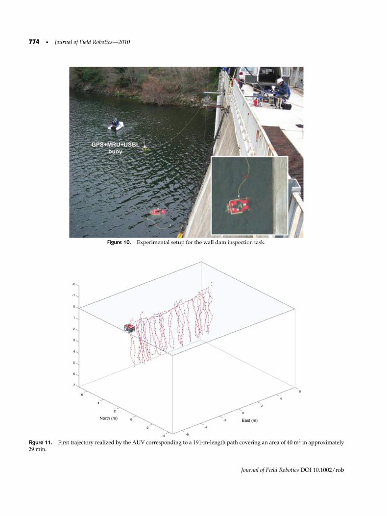
The validation experiments for the proposed system wereperformed during February 2009 in the Pasteral hydroelec-tric dam (Ter River) in Girona (Spain). Figure 10 showsthe experimental setup. The surface buoy, described inSection 2.2, was moored approximately 8 m away from thewall with the transceiver tilted at an angle of 45 deg. A su-pervisory computer was located on top of the dam wall,connected to the buoy through an umbilical cable includ-ing three serial lines (one for the DGPS, one for the USBL,and another for the MRU). Although the robot was con-nected to the supervisory computer through an umbilicalcable providing power and an Ethernet link, it was oper-ated in a totally autonomous mode. The umbilical allowedfor long experiments without worry about battery time.The robot internal variables including the video imageswere monitored through an Ethernet connection. Owing tooperational constraints accorded with the dam owners, andbecause the plant was generating power, during the fieldexperiments the surveyed area was limited to a small arealocated at the left of the penstock pipe–protecting fence,far from the stream generated by its water inlet. Neverthe-less, the area was considered wide enough (about 15 m)for these proof-of-concept experiments. The robot was pro-grammed using MCL (see Algorithm 1) to follow a surveytrajectory in the face of the dam wall. During the experi-ment, the robot used only the onboard navigation systembased on a DVL and a MRU–FOG and the data gatheredfrom the moored buoy (USBL, DGPS, and MRU) were pro-cessed and stored on the supervisory computer and laterused offline to reestimate the trajectory for the global align-ment and georeferencing of the image sequence.

Figure 11 represents the trajectory executed during thesurvey mission. The trajectory consisted of a series of verti-cal movements alternated with lateral displacements while



Figure 10. Experimental setup for the wall dam inspection task.

Figure 11. First trajectory realized by the AUV corresponding to a 191-m-length path covering an area of 40 m2 in approximately29 min.



Figure 12. Globally aligned image mosaic corresponding to the trajectory shown in Figure 11.

maintaining the vehicle perpendicular to the dam’s walland at a constant distance. To avoid holes in the final mo-saic and to ensure covering 100% of the surveyed area withredundant visual data, the vehicle scanned the area fromleft to right and then again from right to left back to thestarting position. Revisiting previously surveyed areas andensuring a good overlapping between adjacent images (al-ways greater than 50%) improves the precision and qual-ity of the final mosaic. The total mission time to execute a40-m2 survey was 29 min. The trajectory (solid line) in thefigure was obtained with the filter described in Section 4, in-corporating the surface buoy position measurements (dots)as explained in Section 4.4 and smoothed as reported inSection 4.5. It is worth mentioning that although the repre-sented data have their origin placed over the surface buoy,the resulting trajectory was obtained in world coordinates.During the execution of the filter, a few surface buoy mea-surements were discarded after being considered as out-liers by the individual compatibility test. Some of them canbe easily spotted on the upper-right corner of the trajectoryas isolated points.

The position data shown in Figure 11 were used to-gether with all the captured images to build the mosaic pre-sented in Figure 12. The mosaic is a high-resolution image,more than 67 Mpx (approx. 1 pixel/ml), including a totalof 1,998 images. In Figure 12, the seam transitions amongthe images as well as strong differences in the illuminationcan be perceived, making visual inspection difficult. Afterthe blending process described in Section 6.7, the resultingimage mosaic (Figure 13) becomes a much clearer image inwhich plenty of algae can be seen on the wall, as well ascircular markers that were added to verify the result. Ad-ditional results can be observed in Figure 14, which showsthe final result corresponding to a second trajectory where,

in the bottom-left corner, rocks can be seen on the floor ofthe reservoir.

The distance between each pair of circular markers at-tached to a rope was known prior to the experiment. Al-though we had no means to precisely survey the exact finalposition of the markers hanging on the wall, we can ap-proximate that the local accuracy of the final mosaic is inthe order of a few centimeters. With respect to the globalposition estimate, the error is largely dependent on the pre-cision of the GPS system mounted on the buoy. With a stan-dard DGPS such as the one used during the trials, a preci-sion of about 2 or 3 m can be expected. The precision of theUSBL while operating in such short range (its maximumoperative range is 1,500 m) should be of a few centimetersand, therefore, insignificant in comparison with the errorscoming from the GPS.

8. CONCLUSIONS

This paper has presented the results of a research projectthat proposes an automated solution to the visual inspec-tion problem of hydroelectric dams. The solution consistsof using a small AUV together with a localization buoy toacquire a set of images, navigation data, and other infor-mation while the robot is autonomously performing a tra-jectory in front of the wall of a dam. After this experimentalphase, all the information is processed in the lab to generatea high-quality georeferenced photomosaic of the inspectedwall.

Results obtained from an experiment conducted inFebruary 2009 at the Pasteral hydroelectric dam demon-strate the feasibility of the system. The results includetwo mosaics of the dam with sufficient resolution (approx.1 pixel/mm) to make possible the detection of damage



Figure 13. Blended image mosaic corresponding to the trajectory shown in Figure 11.

Figure 14. Blended mosaic corresponding to a second trajectory.

in the concrete wall. Unfortunately, because the dam wasgenerating power, it was not possible to perform a surveyof the protecting fence at the water inlet to the penstockgallery. However, this scenario has enough similarities withthe demonstrated mission that we are confident in the ad-equacy of the proposed framework as long as the fence ismassive enough to be detected with the sonar.

In the presented experiments, the surveyed area waslimited to a small portion of the wall (40 m2). Previousworks (Ferrer, Elibol, Delaunoy, Gracias, & Garcıa, 2007)demonstrate the capacity of the proposed mosaicking sys-tem to deal with very large visual maps (about 1 km2).

Therefore, it should be reasonable to assume that the cur-rent system will be capable of generating the mosaic of acomplete dam wall.

The resulting visual map offers several advantageswith respect to the traditional diver/ROV inspection ap-proach. First, the inspection process is systematic and en-sures 100% coverage of the surveyed area. Second, the useof an AUV to perform tasks in such a dangerous environ-ment avoids putting human lives at risk. Also, the resultingmap offers a global view of the area, which simplifies the in-terpretation of the scene. Finally, the georeferencing of themap simplifies the referencing of future surveys and makes



possible determining the exact location where repair workshould take place.

Future work should focus on testing the performanceof the overall system with the objective of determining, andthen improving, the precision of the resulting mosaics. Im-provements in time required to carry out the experiments,in the robustness of the systems, and in the automation ofthe offline processes also point to the economical feasibilityof the method for high-quality visual dam inspection.

APPENDIX: INDEX TO MULTIMEDIA EXTENSIONS

The video is available as Supporting Information in theonline version of this article.

Extension Media type Description

1 Video February 2009 experiments inthe Pasteral hydroelectric dam

ACKNOWLEDGMENTS

The authors wish to thank the Spanish Ministry for fund-ing project DPI2005-09001-C03-01 and also the workers ofEndesa from the Pasteral hydroelectric plant for their col-laboration in the experiments. The project was carried outby members (staff and students) of the Vicorob researchgroup of the University of Girona.

REFERENCES

Antich, J., Ortiz, A., & Oliver, G. (2005). A PFM-based con-trol architecture for a visually guided underwater cabletracker to achieve navigation in troublesome scenarios.Journal of Maritime Research, 2(1), 33–50.

Arkin, R. C. (1998). Behavior-based robotics. Cambridge, MA:MIT Press.

Balasuriya, A., & Ura, T. (2002, October). Vision based under-water cable detection and following using AUVs. In Pro-ceedings of the Oceans MTS/IEEE, Biloxi, MS (pp. 1582–1587).

Batlle, J., Nicosevici, T., Garcıa, R., & Carreras, M. (2003,September). ROV-aided dam inspection: Practical results.In Proceedings of the 6th IFAC Conference on Ma-noeuvring and Control of Marine Crafts, Girona, Spain(pp. 309–312).

Bay, H., Tuytelaars, T., & Gool, L. V. (2006, May). SURF:Speeded up robust features. In European Conference onComputer Vision, Graz, Austria (pp. 404–417).

Bouguet, J. Y. (2010). Camera calibration toolbox for Matlab.http : / / www.vision.caltech.edu / bouguetj / calib doc/index.html. Accessed 20 May 2010.

Brokloff, N. A. (1994, September). Matrix algorithm forDoppler sonar navigation. In Proceedings of the OceansMTS/IEEE, Brest, France (vol. 3, pp. 378–383).

Brown, M., & Lowe, D. G. (2003, October). Recognising panora-mas. In International Conference on Computer Vision,Nice, France (pp. 1218–1225).

Capel, D. P. (2004). Image mosaicing and super-resolution.Heidelberg, Germany: Springer Verlag.

Castellanos, J. A., & Tardos, J. D. (1999). Mobile robot localiza-tion and map building: A multisensor fusion approach.Boston, MA: Kluwer Academic Publishers.

Cote, J., & Lavallee, J. (1995, December). Augmented realitygraphic interface for upstream dam inspection. In Pro-ceedings of SPIE Telemanipulator and Telepresence Tech-nologies II, Philadelphia, PA (vol. 2590, pp. 33–39).

Djapic, V. (2009). Unifying behavior based control design andhybrid stability theory for AUV application. Ph.D. thesis,UC Riverside.

Englot, B., & Hover, F. (2009, October). Stability and robustnessanalysis tools for marine robot localization and SLAM ap-plications. In IEEE/RSJ International Conference on Intel-ligent Robots and Systems, St. Louis, MO (pp. 4426–4432).

Escartın, J., Garcia, R., Delaunoy, O., Ferrer, J., Gracias, N.,Elibol, A., Cufı, X., Neumann, L., Fornari, D. J., Humphris,S., & Renard, J. (2008). Globally aligned photomosaic ofthe Lucky Strike hydrothermal vent field (Mid-AtlanticRidge, 37 ◦18.50N): Release of georeferenced data, mosaicconstruction, and viewing software. Geochemistry Geo-physics Geosystems, 9(12), 1–17.

Eustice, R., Singh, H., Leonard, J., Walter, M., & Ballard, R.(2005, June). Visually navigating the RMS Titanic withSLAM information filters. In Proceedings of Robotics Sci-ence and Systems, Cambridge, MA.

Ferrer, J., Elibol, A., Delaunoy, O., Gracias, N., & Garcıa, R.(2007, September–October). Large-area photo-mosaics us-ing global alignment and navigation data. In Proceedingsof the Oceans MTS/IEEE, Vancouver, Canada (pp. 1–9).

Fischler, M. A., & Bolles, R. C. (1981). Random sample con-sensus: A paradigm for model fitting with applications toimage analysis and automated cartography. Communica-tions of the ACM, 24(6), 381–395.

Fossen, T. I. (1994). Guidance and control of ocean vehicles.Chichester, UK: John Wiley & Sons, Ltd.

Garcia, R., Batlle, J., Cufı, X., & Amat, J. (2001, May). Position-ing an underwater vehicle through image mosaicking. InIEEE International Conference on Robotics and Automa-tion, Seoul, Korea (vol. 3, pp. 2779–2784).

German, C., Yoerger, D., Jakuba, M., Shank, T., Langmuir, C., &Nakamura, K. (2008). Hydrothermal exploration with theautonomous benthic explorer. Deep Sea Research Part I:Oceanographic Research Papers, 55(2), 203–219.

Hagen, P. E., Storkersen, N. J., & Vestgard, K. (1999, December).HUGIN—Use of UUV technology in marine applications.In Proceedings of the Oceans MTS/IEEE, Seattle, WA.

Harris, C. G., & Stephens, M. J. (1988, August–September). Acombined corner and edge detector. In Proceedings of the4th Alvey Vision Conference, Manchester, UK (pp. 147–151).

Hartley, R., & Zisserman, A. (2004). Multiple view geometry incomputer vision. Cambridge, UK: Cambridge UniversityPress.



Kalman, R. E. (1960). A new approach to linear filtering andprediction problems. Transactions of the ASME, Journalof Basic Engineering, 82(Series D), 35–45.

Kazmi, W., Ridao, P., Ribas, D., & Hernandez, E. (2009, May).Dam wall detection and tracking using a mechanicallyscanned imaging sonar. In Proceedings of the IEEE Inter-national Conference on Robotics and Automation, Kobe,Japan (pp. 3595–3600).

Kim, A., & Eustice, R. (2009, October). Pose-graph visual SLAMwith geometric model selection for autonomous under-water ship hull inspection. IEEE/RSJ International Con-ference on Intelligent Robots and Systems, 2009. IROS2009, St. Louis, MO (pp. 1559–1565).

Leonard, J. J., & Durrant-Whyte, H. F. (1992). Directedsonar sensing for mobile robot navigation. Norwell, MA:Kluwer Academic Publishers.

Leonard, J. J., & Rikoski, R. J. (2001). Incorporation of de-layed decision making into stochastic mapping (vol. 271,pp. 533–542). Heidelberg, Germany: Springer Verlag.

Mindell, D., & Bingham, B. (2001, November). New archaeo-logical uses of autonomous underwater vehicles. In Pro-ceedings of the Oceans MTS/IEEE, Honolulu, HI.

Murata, T. (1989). Petri nets: Properties, analysis and applica-tions. Proceedings of the IEEE, 77(4), 541–580.

Negahdaripour, S., & Firoozfam, P. (2006). An ROV stereo-vision system for ship-hull inspection. IEEE Journal ofOceanic Engineering, 31(3), 551–564.

Nicosevici, T., Gracias, N., Negahdaripour, S., & Garcıa, R.(2009). Efficient three-dimensional scene modeling andmosaicing. Journal of Field Robotics, 26(10), 759–788.

Palomeras, N., Ridao, P., Carreras, M., & Silvestre, C.(2008, July). Towards a mission control language forAUVs. In 17th IFAC World Congress, Seoul, Korea (pp.15028–15033). The International Federation of AutomaticControl.

Palomeras, N., Ridao, P., Carreras, M., & Silvestre, C. (2009,October). Using Petri nets to specify and execute mis-sions for autonomous underwater vehicles. In Interna-tional Conference on Intelligent Robots and Systems, St.Louis, MO (pp. 4439–4444).

Petillot, Y., Reed, S., & Bell, J. (2002, October). Real time AUVpipeline detection and tracking using side scan sonar andmulti-beam echo-sounder. In Proceedings of the OceansMTS/IEEE, Biloxi, MS (vol. 1, pp. 217–222).

Pizarro, O., Eustice, R., & Singh, H. (2004, November). Largearea 3D reconstructions from underwater surveys. InMTS/IEEE OCEANS Conference, Kobe, Japan (vol. 2,pp. 678–687).

Pizarro, O., & Singh, H. (2003). Toward large-area mosaic-ing for underwater scientific applications. IEEE Journal ofOceanic Engineering, 28(4), 651–672.

Poupart, M., Benefice, P., & Plutarque, M. (2001, Septem-ber). Subacuatic inspections of EDF (Electricite de France)dams. In OCEANS, 2000. MTS/IEEE Conference and Ex-hibition, Providence, RI (vol. 2, pp. 939–942).

Prados, R. (2007). Image blending techniques and their applica-tion in underwater mosaicing. Master’s thesis, Universityof Girona.

Ribas, D., Neira, J., Ridao, P., & Tardos, J. (2006, September).AUV localization in structured underwater environmentsusing an a priori map. In Proceedings of the 7th IFAC Con-ference on Manoeuvring and Control of Marine Crafts,Lisbon, Portugal.

Ribas, D., Palomer, N., Ridao, P., Carreras, M., & Hernandez, E.(2007, April). Ictineu AUV wins the first SAUC-E competi-tion. In Proceedings of the IEEE International Conferenceon Robotics and Automation Rome, Italy (pp. 151–156).

Ribas, D., Ridao, P., & Neira, J. (2010). Underwater SLAMfor structured environments using an imaging sonar.Number 65 in Springer Tracts in Advanced Robotics.Heidelberg, Germany: Springer Verlag.

Ribas, D., Ridao, P., Tardos, J., & Neira, J. (2008). UnderwaterSLAM in man-made structured environments. Journal ofField Robotics, 25(11–12), 898–921.

Ridao, P., Batlle, E., Ribas, D., & Carreras, M. (2004, Novem-ber). NEPTUNE: A HIL simulator for multiple UUVs. InProceedings of the Oceans MTS/IEEE, Kobe, Japan (vol. 1,pp. 524–531).

Salamin, E. (1979). Application of quaternions to computationwith rotations (Tech. Rep.). Stanford University, Stanford,CA.

Seabotix, Inc. (2010). Seabotix, Inc.—Hydro applications.http://www.seabotix.com/applications/hydro.htm. Ac-cessed 3 April 2010.

Singh, H., Roman, C., Pizarro, O., Eustice, R., & Can, A. (2007).Towards high-resolution imaging from underwater vehi-cles. International Journal of Robotics Research, 26(1), 55–74.

Smith, R., Self, M., & Cheeseman, P. (1990). Estimating uncer-tain spatial relationships in robotics. In Autonomous robotvehicles (pp. 167–193). New York: Springer-Verlag NewYork, Inc.

Tao. (2003). TAO developer’s guide version 1.3a, volume 2. St.Louis, MO: Object Computing, Inc.

Thrun, S., Burgard, W., & Fox, D. (2005). Probabilistic robotics.Cambridge, MA: MIT Press.

Triggs, B. (1998, June). Autocalibration from planar scenes. InProceedings of the 5th European Conference on ComputerVision, Freiburg, Germany (vol. 1, pp. 89–105).

Triggs, B., McLauchlan, P., Hartley, R., & Fitzgibbon, A. (2000).Bundle adjustment—A modern synthesis. In W. Triggs,A. Zisserman, and R. Szeliski (Eds.), Vision algorithms:Theory and practice, Lecture Notes in Computer Science(pp. 298–375). London: Springer Verlag.

VideoRay LLC. (2010). VideoRay LLC—Hydro inspection.http://www.videoray.com/missions/23. Accessed 3April 2010.

Vincent, E., & Laganiere, R. (2001, June). Detecting planar ho-mographies in an image pair. In IEEE Symposium on Im-age and Signal Processing and Analysis, Pula, Croatia(pp. 182–187).

Williams, S., & Mahon, I. (2004, April–May). Simultaneous lo-calisation and mapping on the Great Barrier Reef. In Pro-ceedings of the IEEE International Conference on Roboticsand Automation, New Orleans, LA (vol. 2, pp. 1771–1776).


visual inspection of hydroelectric dams using an …eia.udg.edu/~rafa/papers/jfr2010b.pdf · ·...

Documents