Visual LinProg: A Web-based Educational Software for Linear Programming VASSILIOS LAZARIDIS, KONSTANTINOS PAPARRIZOS, NIKOLAOS SAMARAS∗, ANGELO SIFALERAS Department of Applied Informatics, University of Macedonia, 156 Egnatias Str., 54006 Thessaloniki, Greece.

ABSTRACT: Visual LinProg is an educational tool that solves Linear Problems (LPs) using animation and visualization techniques. The core of the proposed software includes the well-known class of simplex type algorithms. This tool is a Web-based software and hence platform independent. Visual LinProg was initially invented to be used in mathematical programming courses to supplement the teaching. The user-student can solve his own general LPs, view the solution process step-by-step and import or export his own examples in an easy way to read format. The solution process is covered scholastically through textual information and also the necessary steps from the pseudo code are depicted using multiple views. In this paper we describe Visual LinProg and how it is used in educational purposes. Finally, we present an evaluation of the proposed educational tool. Keywords: Computers and Education, Educational Software Implementation, Linear Programming, Java.

1. INTRODUCTION Recently, there has been a growing interest in the developing of educational software [1]. World Wide Web has given many new features in the educational process. Web based learning tools have become the focus of research in the last 10 years. In order to develop educational software it is very important to have good programming background. The usage of visualization and animation techniques offers the change to actively engage the students in the learning process.

Linear Programming is perhaps the most important and well studied optimization problem. Lots of real world problems can be formulated as linear programming problems. One of the challenging aspects of teaching a course in Linear

∗ Corresponding author. Tel.: +302310 891866, fax: +302310 891879. E-mail address: vlaz@kozani.teikoz.gr (V. Lazaridis), paparriz@uom.gr (K. Paparrizos), samaras@uom.gr (N. Samaras), sifalera@uom.gr (A. Sifaleras)

LAZARIDIS ET AL.

Programming is teaching students about the details of different solution techniques (algorithms) and how sensitive is the optimal solution.

Linear Programming consists of optimizing, minimizing or maximizing, a linear function over a certain domain. The domain is given by a set of linear constraints. Simplex type algorithms are the most common tool for the solution of LP’s. These algorithms are by nature complicated to understand and to teach. Roughly speaking, the major objective of a course intended to teach Linear Programming is that the students are familiarized with the main notions, and understands some basic operation of Linear Algebra. The fundamental concepts of Simplex type algorithms, drastically affect the thorough understanding of other Linear Programming algorithms. The study of appropriate examples has proved, so far, to be a key issue during the learning process. Mathematical formulation, the choice of the most suitable algorithm for the solution and the interpretation of the results constitute the necessary steps of the optimization problems.

In the end of the course, the students should be able to solve small-scale LPs by hand.

The learning of Simplex type algorithms shows many difficulties, whether the students come from Mathematics Departments or Computer Science Departments. Teaching Linear Programming using spreadsheets can be further improved with the incorporation of graphical solution [2, 3, 4]. There are many cases, where the visualization techniques have assisted a lot wherever the textual solution has failed [5]. Visualization of simplex type algorithms can assist the instructor to illuminate their description and to graphically show topics that he explained on the blackboard.

World Wide Web has given advances in the education of Linear Programming. The aim of the development of NEOS Guide [6] was to provide information and educational software about optimization. Creating a Simplex applet with the capability of inserting a problem and the surveillance of all the steps for the solution of the problem is a tool exclusively for educational purposes. The usage of Web technologies, even if is not suitable for every aspect of optimization applications [7] make clear the positive impact in Operations Research and the Management Science.

This study is organized as follows. Following this introduction, in section 2 we present related work and some on-line software. In section 3 we give a brief description of the revised simplex algorithm. In the section 4 some implementation issues are discussed. A sort description of the proposed software is presented in section 5 and 6. Section 7 contains the evaluation of Visual LinProg. Finally, in section 8 we conclude. 2. RELATED WORK AND ON-LINE SOFTWARE World Wide Web makes it possible for any instructor to access information relevant to Linear Programming, but it provides also the possibility to find freeware LP solvers or educational software. The main feature of those Web based applications is the interaction with the user in order to solve a LP. All these previously mentioned applications can be divided into two categories, depending on the way the solution is being presented: (i) applications based on graphical solution (representation in 2D or 3D) and (ii) applications based on Simplex algorithmic solution.

Some common features among these applications are the ability to solve problems only of limited size, they focus in the visualized solution of the LP and finally they are mostly used in the educational field. The optimization software which

VISUAL LINPROG

is designed for academic usage centres usually to a few algorithms and are devised for deeper comprehension of new algorithms.

In the following subsections we briefly discuss the above two categories. 2.1 Applications based on graphical solution The fundamental problem as far as the graphical solution is concerned, is the limitation to one, two or three decision variables. Graphical solution provides a clear depiction of all the vertices as also the feasible and infeasible area. Through this method, it can be learned that whenever a LP has limited feasible area it follows that the optimal solution is one of the feasible area’s vertices. These applications enable the student to insert customizable LP, but without giving the necessary steps, they show the feasible region and the optimal solution.

Some characteristic applications which show the graphical solution through World Wide Web, for educational reasons came from [8] and Anima - LP: A Tool for teaching Linear Programming [9]. LP-Explorer [10], shows not only the graphical solution, but go a step forward with the algorithmic solution using the Simplex method with tableau format. 2.2 Applications based on Simplex algorithmic solution Simplex type algorithms are the most known methods for the solution of LP. During the process of solution they move from one feasible point to another adjacent until an optimal solution has been reached. Most on-line applications don’t show beyond the calculations of the solution procedure.

There are two kinds of solutions presentation: (i) Tableau format and (ii) Revised form. The solution based on the tableau format is more widespread through the educational community and it is easier at the calculation (by hand). Moreover, this way the solution relies only at elementary row operations. Some applications which belong to this category are of [11] which allow the selection of the Primal Simplex or Dual Simplex as a main solver. In addition, there exists also a well known application [12], which also gives user the choice for the solver. The solution based on the revised form demands greater effort from the user. Especially in cases where the problem involves three constraints the calculation by hand prove to be very hard. Usually the presentation and the teaching of the Simplex method, using the revised, are avoided in undergraduate level. Applications demonstrating the solution using revised form include [13], while the software in [14] allows the selection from a large number of LP algorithms. 3. DESCRIPTION OF THE SOLVING ALGORITHMS We are concerned with the following LP notation

min. .

x 0

Tc xs t Ax b=

≥ (LP.1)

where s.t. stands for “subject to”, c, x ∈ℜn, b ∈ ℜm, A ∈ ℜmxn and T denotes matrix or vector transpose.

LAZARIDIS ET AL.

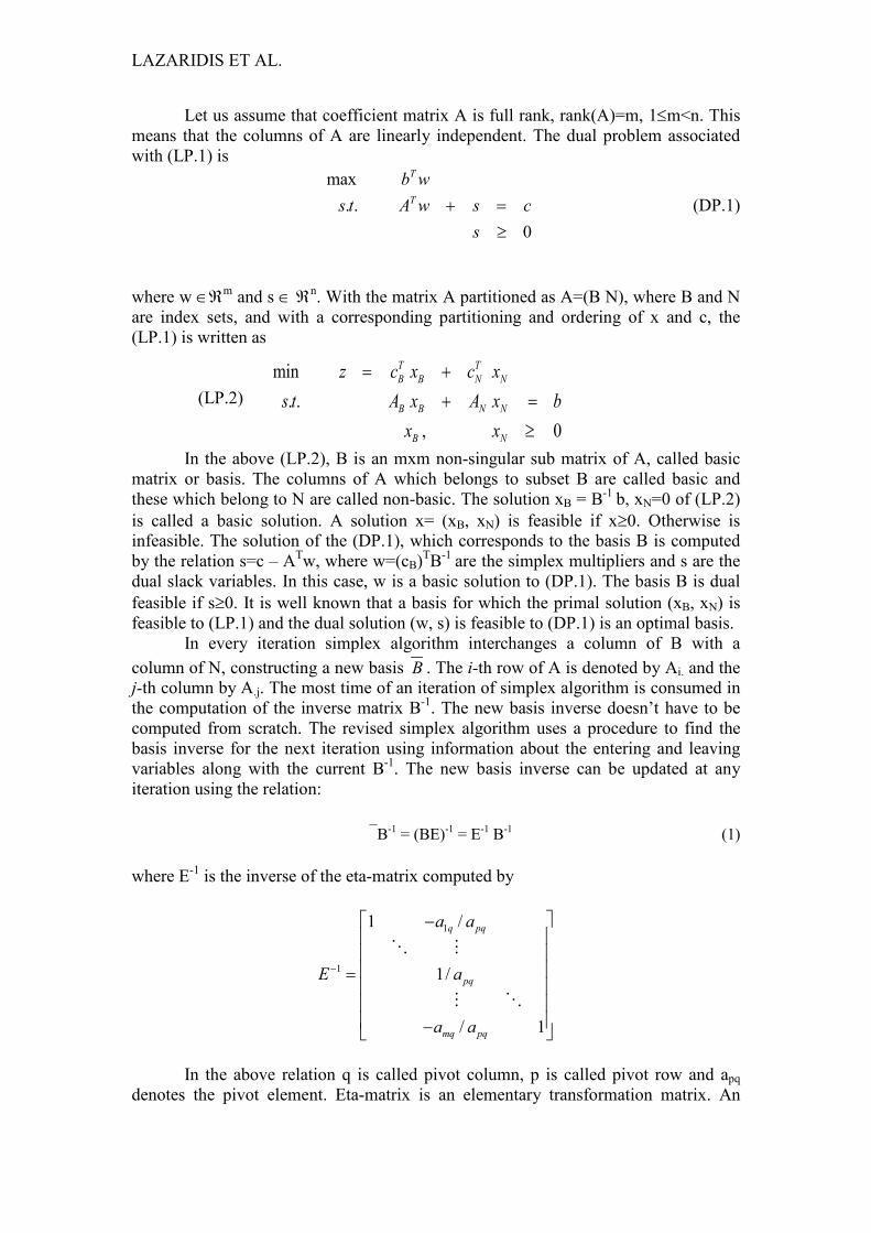
Let us assume that coefficient matrix A is full rank, rank(A)=m, 1≤m<n. This means that the columns of A are linearly independent. The dual problem associated with (LP.1) is

max. .

0

T

T

b ws t A w s c

s+ =

≥ (DP.1)

where w ∈ℜm and s ∈ ℜn. With the matrix A partitioned as A=(B N), where B and N are index sets, and with a corresponding partitioning and ordering of x and c, the (LP.1) is written as

(LP.2)

In the above (LP.2), B is an mxm non-singular sub matrix of A, called basic matrix or basis. The columns of A which belongs to subset B are called basic and these which belong to N are called non-basic. The solution xB = Β-1 b, xN=0 of (LP.2) is called a basic solution. A solution x= (xB, xN) is feasible if x≥0. Otherwise is infeasible. The solution of the (DP.1), which corresponds to the basis B is computed by the relation s=c – ATw, where w=(cB)TB-1 are the simplex multipliers and s are the dual slack variables. In this case, w is a basic solution to (DP.1). The basis B is dual feasible if s≥0. It is well known that a basis for which the primal solution (xB, xN) is feasible to (LP.1) and the dual solution (w, s) is feasible to (DP.1) is an optimal basis.

In every iteration simplex algorithm interchanges a column of B with a column of N, constructing a new basis B . The i-th row of A is denoted by Ai. and the j-th column by A.j. The most time of an iteration of simplex algorithm is consumed in the computation of the inverse matrix B-1. The new basis inverse doesn’t have to be computed from scratch. The revised simplex algorithm uses a procedure to find the basis inverse for the next iteration using information about the entering and leaving variables along with the current B-1. The new basis inverse can be updated at any iteration using the relation:

Β-1 = (ΒΕ)-1 = Ε-1 Β-1 (1) where Ε-1 is the inverse of the eta-matrix computed by

1

1

1 /

1/

/ 1

q pq

pq

mq pq

a a

E a

a a

−

− = −

In the above relation q is called pivot column, p is called pivot row and apq

denotes the pivot element. Eta-matrix is an elementary transformation matrix. An

min. .

, 0

T TB B N N

B B N N

B N

z c x c xs t A x A x b

x x

= + + =

≥

VISUAL LINPROG

elementary matrix is a square (mxm) matrix that differs from the identity in only one column. Now we can proceed with a formal description of revised simplex algorithm: Algorithm 1 Revised Simplex Algorithm Require: A feasible basic partition (B,N) Step 0 (Initialization) Compute the matrix B-1 and vectors xB, w, sN. Step 1 (Test of Optimality) if sN≥0 then

STOP. The problem is optimal. else Using a pivoting rule choose the index l of the entering variable

Variable xl enters the basis.

Step 2. (Minimum ratio test) Compute the pivot column hl = B-1A.l. if the hl≤0 then STOP. The problem is unbounded. else Compute:

[ ] [ ][ ] min : 0 B r B i

B r ilrl il

x xx h

h h

= = >

Variable xB[r]= xk is the leaving variable. Endif

Step 3. (Pivoting) Swap indices k and l. Update the new basis inverse

1B

−, using equation (1)

Compute the vectors xB, w, sN. Go to Step 1. endif In order to solve a general linear programming problem of the form

min. .

x 0

Tc xs t Ax b⊗

≥ (LP.3)

where ⊗={≤, =, ≥}and an easily computed basic feasible solution x≥0 doesn’t exist; two methods can be applied. These two methods big-M method and two-phase method can be used in order to find an initial basic feasible solution. A detailed description of these methods can be found in [15]. If the initial solution is dual feasible, then the Dual Simplex algorithm can be applied in the (LP.3). In the flowchart of figure 1, we present the method’s choice procedure.

LAZARIDIS ET AL.

Figure1. Flowchart of method’s choice procedure. 4. IMPLEMENTATION ISSUES This is the first time that such an analytical animation of the simplex type method algorithms in the revised form is being implemented. All the pivots as also the basis formulation are fully animated. Furthermore, it is the first time that using a web accessible tool there is the possibility to import or export whichever example, fully customizable by the user. This is very important, because there are not just a common predefined set of examples which does not cover all the times the interest of the students. Finally, all the implemented methods (Two Phase or Big M method) are also fully detailed, in order for the user to completely comprehend them.

The studies [13] and [16] were a motivation to us for the development of web-based educational software. Visual LinProg has been built using the Java programming language. Java applets can be used for the development of platform - independent applications. This is very convenient in obtaining interaction with the user, through a browser, in any platform. It is executed as any other Java Applet, using Microsoft Internet Explorer (version 4 and above). The only requirement is for the Java Virtual Machine to be previously installed, which is crucial for the execution of Java programs. The screen resolution should be at least 1024 x 768, which is also the default resolution required for the best view of the application. The ability to implement the Simplex type algorithms, for the solution of user defined LPs and the understanding of the results, are the desired scope of every educational procedure.

The main goal is the development of an educational interactive tool which may be used firstly for the teaching inside the classroom/laboratory and secondly as an educational supplement at the student’s home. The application gives the possibility to the student to reach the arithmetic solution of the problem, while avoiding many hard calculations. This way he can focus on working on the thorough understanding of the solution procedure. Furthermore, there is the capability of solving many and difficult user defined linear problems, while eliminating the numerical errors. Apart

VISUAL LINPROG

from the solution of a user defined LP, the proposed software can help the user - student in the following questions:

• How much will the solution be affected, if one or more technological constraints were added? The user can make the appropriate changes and see how the solution changes without filling again all the other values from scratch. • What will happen, if one or more decision variables would be added? Again the user can make the necessary changes and watch how the solution changes without modifying again all the other values from scratch. • Does the optimal solution remain as it is, in case some right hand side values will be changed? • Does the optimal solution remain as it is, in case some reduced cost values will be changed?

Emphasis was given at the final design of the application, to adopt an easy graphical interface for the user and not burden him with the additional learning of a complicated environment. Moreover, the user should have the ability to easily execute the proposed application, without the installation of extra applications in his PC. During the development of this software, the following details were taken account of:

• Observation of the pseudo code. • Analytical presentation of the Simplex algorithm’s mathematical calculations. • Use of Visualization techniques (color, animation, e.t.c.). • Ability of execution of the simplex algorithm, per iteration. • Showing of explanatory additional comments in text format, for every step of the Simplex algorithm. 5. DESCRIPTION OF Visual LinProg The application is suited not only for the novice users but also for the accustomed in the use of visualization tools. The fact that the interactive environment was intended to be very simple, has played a very important role in the design of the proposed application, in order to avoid complicated systems which might confuse students. The student can choose from the environment only basic functions, like for example insertion or solution. The presentation of the solution is accomplished through a Graphical User Interface (G.U.I.), in order that the required mathematical symbols to be shown into a common and easy to understand, by the user, format.

The graphical interpretation of a LP can be done in two modes: i) direct and ii) step-by-step. In the direct mode, the selected algorithm is executed continuously until an answer (optimal, unbounded, and infeasible) is produced. This mode gives to the user an intuitive knowledge of the topic with a quick view. In the step-by-step mode the selected algorithm is executed from step 0 to 3 (see Algorithm 1) and every computation is graphically visualized. Using this mode, students can take deep insight of all computations needed for the solution of a LP. The learning rhythm depends on the students, as they have the control on this mode. They decide the time to dedicate for understanding the transition between steps.

The graphical environment of Visual LinProg consists of the following elements shown in Figure 2.

LAZARIDIS ET AL.

Figure 2. Graphical Interface of Visual LinProg.

• In the Menu bar, the user can choose some basic operations, such as LP insertion, algorithm selection etc. • In the main window, which comprises the basic workspace, all the calculations take place. All these calculations, necessary for the solution of a LP, contain computations, visualization and animation. • In the Pseudo-code window, the appropriate pseudo-code is displayed. In the step-by-step mode the command line corresponding to the algorithm being executed is emphasized in red color. • In the Comments window, explanatory messages about the solution process are displayed. • In the Control buttons window the user can control the execution of the selected algorithms. Visual LinProg features the following characteristics: • Choice of prepared LPs • Insertion of LPs from a file • Saving LPs to a file • Saving all the solution steps to a file • Saving only the results to a file • Selection of auxiliary tools: such conversion of a LP into the typical form, transformation of a LP into its equivalent dual form, showing the computation of the basis inverse B-1. 5.1 Insertion of a user defined LP There are five prepared paradigms, included in the Visual LinProg, which can be selected for solution and additionally there is the capability to insert a user defined LP. The selection of a linear LP can be made through the menu Insert, as it can be seen from Figure 3.

VISUAL LINPROG

Figure 3. Insertion menu of a LP.

From the appearing dialogue box, (Figure 4), the user can insert a LP. The maximum dimension of a LP, which can be solved using this tool, is five decision variables and four technological constraints, while on the other hand the minimum dimension should consist of two decision variables and two technological constraints.

The values belonging to the coefficient matrix A, to the cost c vector and to the right hand side b vector should be in the range [-999.99, 999.99]. The limitations of the dimension of the LP problem and of the range of the coefficients are due to the desired size of the characters at the graphical depiction.

After the insertion of a new LP, the user is able to ask for the solution, pressing the button “Run” (Figure 4). In case the user inserts a LP with dimension mxn, where m = 4 and n = 5, the application calculates automatically it’s dimension. The blank rows and columns in the dialogue box (Figure 2), are ignored from the application. In case where a coefficient is equal to zero, there is no need to be inserted.

Figure 4. Dialogue box for an insertion of a LP.

LAZARIDIS ET AL.

The application automatically fills the blank positions with zeros. The possible faults which might occur, during the insertion of a new LP, are the following: • The objective function has not been defined yet. So it holds that cj = 0, j =1, 2, ..., n. • The number of decision variables is less than two. So it holds that n < 2. • The number of constraints is less than two. So it holds that m < 2. • If any of the coefficients of the new LP, does not belong in the appropriate range of values [-999.99,999.99]. So it holds that cj, bj, Aij ∉[−999.99, 999.99], i, j = 1, 2, ..., n • If a decision variable, which in the coefficient matrix has values equal to zero, has been defined. So it holds that cj = 0 and A.j = 0, ∀ j = 1, 2, ..., n

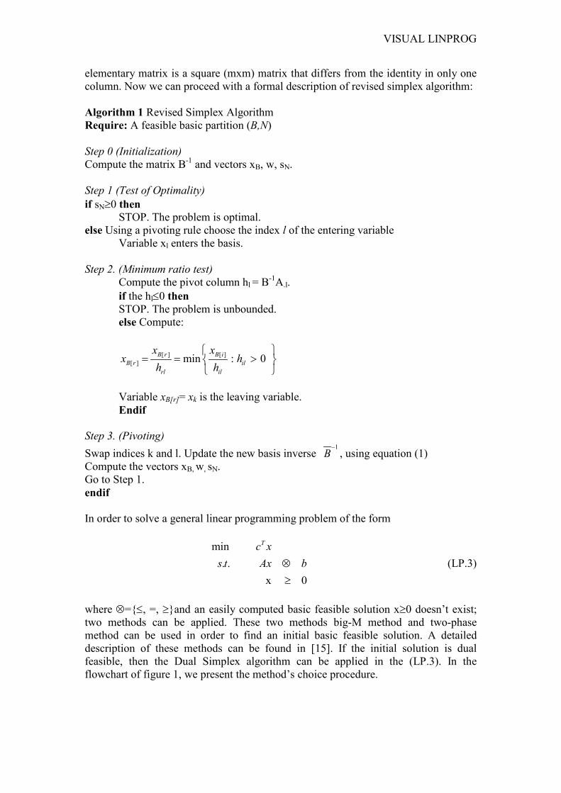
At any point, the insertion of a new problem can be paused. The dialogue box of the insertion of a new problem closes after pressing the “Exit” button. After the insertion of the linear problem, which is being shown in the mathematical form in the application’s window (Figure 5), the user might ask for the solution of the linear problem.

Figure 5. Mathematical formulation of the new linear problem 5.2 Solution of a LP There are two optional ways for the solution of a LP: • Using the “Run” button (direct mode) (Figure 6), the Simplex algorithm starts and runs continuously till the final solution (if exists) of the problem, without the option of observation of all the intermediate steps. • Using the “Next Step” button (step-by-step) (Figure 6), the Simplex algorithm starts and runs step by step, till it terminates.

Figure 6. The control buttons.

In the step-by-step solution of the linear problem, after each step the algorithm pauses and the application is waiting from the user to continue by pressing the “Next Button”. During the step-by-step execution of the algorithm, at the steps where

VISUAL LINPROG

animation exists, the delay of the movement is defined from the pull down menu, through the time switch. By default, the delay has been defined to 10 msec (slow animation). Alternatively, the times 5 msec and 1 msec could be also choosed. At whatever point, by pressing the “Next Step”, the animation stops and the next step of the algorithm is executed.

The “Stop” button activates only at the duration of the step-by-step execution. The specific button can finalize the execution of the algorithm at any time. The application, after the abortion, turns back at the initial state and the solving procedure sets off again. 5.3 An Illustrative Example In order to demonstrate Visual LinProg in a better way, the solution of an illustrative example will be shown.

After the addition of the slack variables, see Figure 7, the basic data which the algorithm is going to use, like for example the matrices A, B, N and the c, b vectors, should be defined in order for the algorithm to get started.

Figure 7. Creation of feasible basic partition. The selection of the entering variable, see Figure 8, specifies which variable,

at the next iteration, will become basic. This choice is based on the well known Dantzig’s pivoting rule. In order to achieve better understanding, the entering variable is depicted using red colour. The selection of the leaving variable, see Figure 9, is based upon the well-known minimum ratio test. After the choice of both the entering and the leaving variables, the pivoting element is shown.

LAZARIDIS ET AL.

Figure 8. Choice of the entering variable.

Figure 9. Choice of the leaving variable.

VISUAL LINPROG

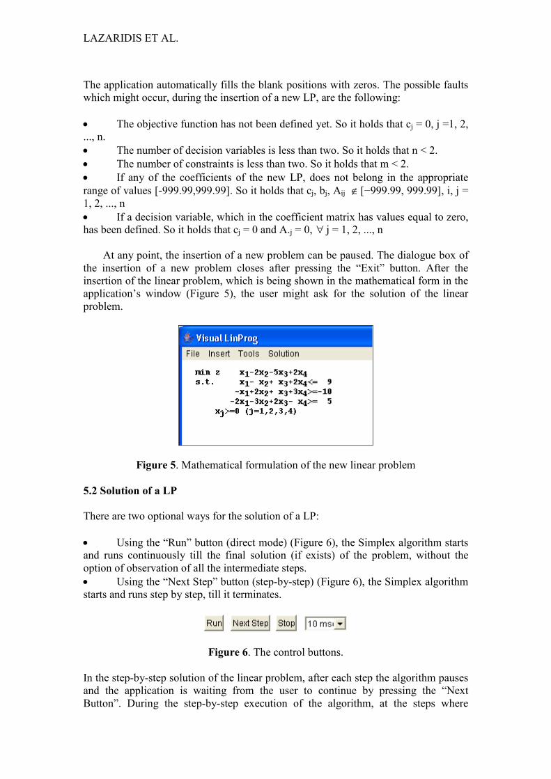
Perhaps, the most difficult point during the solution of linear problems, is the calculation of the basis inverse matrix B−1, see Figure 10. The proposed educational software uses the Eta matrix in order to update basis inverse.

Figure 10. The update procedure of the basis inverse, B−1.

The last step for the completion of the iteration is the creation of the new basic partition. The updates of the data are presented using animation techniques.

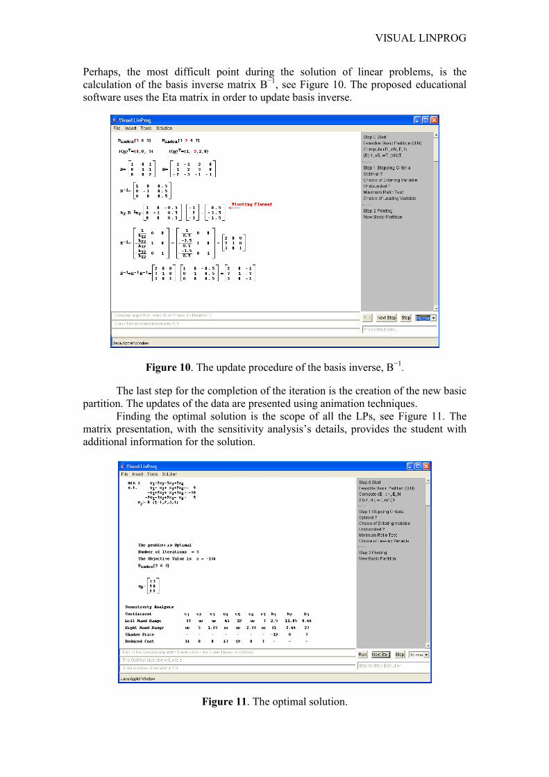
Finding the optimal solution is the scope of all the LPs, see Figure 11. The matrix presentation, with the sensitivity analysis’s details, provides the student with additional information for the solution.

Figure 11. The optimal solution.

LAZARIDIS ET AL.

6. FILES MANAGEMENT Java applets are included in an HTML web page, which are transferred through the HTTP protocol from a Web server. Due to security related reasons, access on local storage devices is restricted. When the code is being loaded, the permission is determined from the pre - defined safety policy. The safety policy decides which access permissions are available for the code being executing. If no permission has been granted to the code, it cannot have access to a guarded resource. All these new concepts of access and policies, gives Java 2 Platform the opportunity to control the access, [17]. The application provides only the option to insert a file containing a LP problem. These textual files have a .lp extension and have also a special format. The application provides the ability, besides the saving of the LP problem files, also the saving either of the final result or of all the solution steps of the LP problem.

Saving the results, comprises of the following details, which were calculated at the termination of the solving algorithm. Those details are: the initial problem, the result from the algorithm’s execution, (optimal, unbounded, infeasible), the total number of iterations, the basic variables and their corresponding values, the optimal objective value, (in case of optimality), the name of the algorithm which was used for the solution, the sensitivity analysis, if it has been asked from the user to be calculated.

The saving of all the solution steps, gives us the ability to save all the actions, which were needed for the solution of the LP problem. Only during the step-by-step solution, all the solution steps are saved, except the previous ones. This way, all the steps are saved; analytically with the calculations needed for the solution. 6.1 The format of the result files The representation of the mathematical symbolisms, which the students are familiar with, aids a lot firstly at the presentation and secondly at the use of the computers. For instance Mathematical Markup Language, [18], is a World Wide Web Consortium (W3C) specified language for expressing mathematics and an XML application for mathematical equations. There are several different ways that it can be used, depending upon the browser and/or plug-in that the user may use.

The main format of the file is XHTML + MathML, which resembles to a Web page (HTML), but contains also functions for the description of mathematical symbols using MathML. In order for a file to be read, Internet Explorer version 5.5 or newer and MathPlayer application must be used.

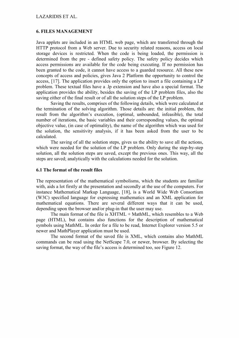
The second format of the saved file is XML, which contains also MathML commands can be read using the NetScape 7.0, or newer, browser. By selecting the saving format, the way of the file’s access is determined too, see Figure 12.

VISUAL LINPROG

Figure 12. Result file in html format.

7. Visual LinProg EVALUATION Researches have shown that it is more significant to find how students use this specific software, rather than just explaining what this educational tool shows them [19]. Feedback from students is necessary to tune up the best possible application.

Therefore, the Visual LinProg was tested thoroughly inside the classrooms during the lectures, for the needs of the course “Linear Optimization Algorithms” at the Department of Applied Informatics, of the University of Macedonia. Besides, there have been conducted researches which support that pedagogical advantages can be only partially attributed to Algorithm Visualization Technology, as for example [20].

For these reasons, a questionnaire was handed out to the 43 students, who attended the specific course. Based on the feedback of these students, a short statistical analysis was carried out, in order to clarify the benefits or the drawbacks of this tool. The questionnaire consisted of 19 questions.

Some of them examine the experience of the students regarding visualization tools. Others examine the usability of the Simplex animation software and finally other require from the students to discuss the potential of the proposed software, (requests for further development, etc.).

In order to present the most important results of the questionnaire, five questions were decided for inclusion in this section. The following drawings present the histograms and some frequency tables of the specific questions.

To start with, the 2nd question was “What do you prefer in order to understand the operation of the Simplex algorithm? a) You learn the pseudo code, b) You create a diagram, or c) You solve many examples”. As show by the responses in Figure 13 the majority of the students prefer to solve many examples, than merely to learn the pseudo code or create diagrams. Therefore, the proposed applet can prove useful to them in solving their own customizable problems. The 10th question was “Did the Simplex Animation software helped you, in the understanding of the Linear

LAZARIDIS ET AL.

Optimization concepts?”. The mean value of the answers was 3.44, as it is shown in Figure 14. This way, the previous statement, (regarding the software usability), can be verified now.

Figure 13. The histogram and frequencies table based on the 2nd question.

05

1015

20

1 2 3 4 5

Satis faction

Freq

uenc

y

Figure 14. The histogram and frequencies table based on the 10th question.

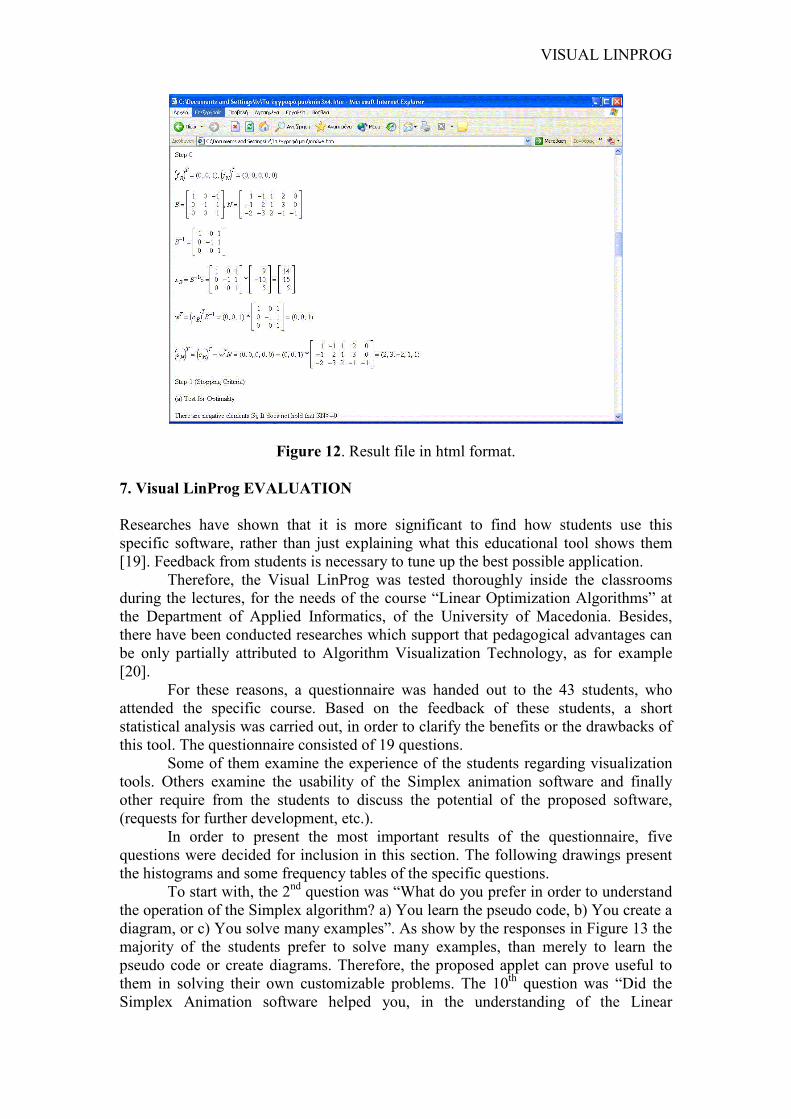
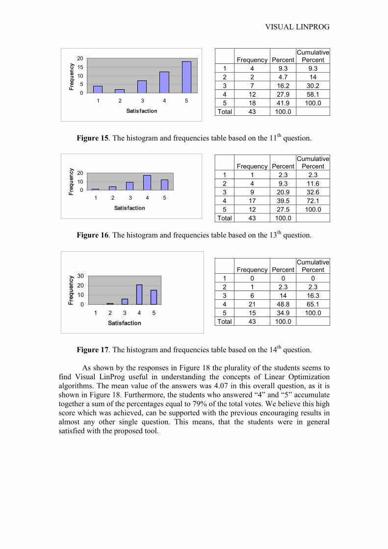
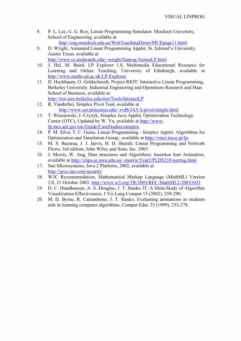
The 11th question was “Determine how much “user - friendly”, the Visual LinProg software is”. The mean value of the answers was 3.88. Due to the educational aspect of the Visual LinProg applet, enough consideration was given in designing a friendly G.U.I. The students, as shown by their opinions in Figure 15, managed to handle easily and efficiently the application in short time. The 13th question was “During the solution of a problem, using the proposed tool, does the animation of the pseudo - code steps, assists in the comprehension of the Linear Programming topics?”. The mean value of the answers was 3.81. The results in Figure 16 show that the animation of the pseudo - code steps as used in our applet, plays a very important factor. The majority of the students, preferred to see simultaneously the pseudo code, in order to remember the steps. Finally, the 14th question was “During the solution of a LP using the Visual LinProg animation software, does the textual description aids in your comprehension of the Simplex algorithm functionality?”. The mean value of the answers was 4.16. Finally, as it seems from Figure 17, the textual description helps the student to clarify the details of the algorithm in a better way. The view of all the necessary computations and the updates of all the matrices, aids in their understanding of the Simplex algorithm functionality.

Frequency Percent Cumulative Percent

Study Pseudo Code

12 27.9 27.9

Create diagrams 5 11.6 39.5

Solve many examples 26 60.5 100.0

Total 43 100.0

Frequency Percent Cumulative

Percent 1 4 9.3 9.3 2 3 7 16.3 3 13 30.2 46.5 4 16 37.2 83.7 5 7 16.3 100.0

Total 43 100.0

05

1015202530

StudyPseudoCode

Creatediagrams

Solve manyexamples

Freq

uenc

y

VISUAL LINPROG

05

101520

1 2 3 4 5

Satis faction

Freq

uenc

y

Figure 15. The histogram and frequencies table based on the 11th question.

01020

1 2 3 4 5

Satis faction

Freq

uenc

y

Figure 16. The histogram and frequencies table based on the 13th question.

0102030

1 2 3 4 5

Satisfaction

Freq

uenc

y

Figure 17. The histogram and frequencies table based on the 14th question.

As shown by the responses in Figure 18 the plurality of the students seems to find Visual LinProg useful in understanding the concepts of Linear Optimization algorithms. The mean value of the answers was 4.07 in this overall question, as it is shown in Figure 18. Furthermore, the students who answered “4” and “5” accumulate together a sum of the percentages equal to 79% of the total votes. We believe this high score which was achieved, can be supported with the previous encouraging results in almost any other single question. This means, that the students were in general satisfied with the proposed tool.

Frequency Percent Cumulative

Percent 1 4 9.3 9.3 2 2 4.7 14 3 7 16.2 30.2 4 12 27.9 58.1 5 18 41.9 100.0

Total 43 100.0

Frequency Percent Cumulative

Percent 1 1 2.3 2.3 2 4 9.3 11.6 3 9 20.9 32.6 4 17 39.5 72.1 5 12 27.5 100.0

Total 43 100.0

Frequency Percent Cumulative

Percent 1 0 0 0 2 1 2.3 2.3 3 6 14 16.3 4 21 48.8 65.1 5 15 34.9 100.0

Total 43 100.0

LAZARIDIS ET AL.

0

5

10

15

20

1 2 3 4 5

Satisfaction

Freq

uenc

y

Figure 18. The histogram and frequencies table based on the 9th question 8. CONCLUSIONS Visual LinProg is web-based educational software. It was initially designed to be used in Linear Programming courses for teaching simplex type algorithms. Visual LinProg is a supplement tool that provides to the student both a theoretical and practical learning of the principles of linear programming inside a graphical environment that can be executed via Internet. The animation of simplex type algorithms code along with its visual animation gives the student an explanation of each step as it is being carried out. Visual LinProg can be used in two ways. First, the introductory while explaining simplex type algorithm, can focus at each step and addressing student questions. Second, the student can solve his own examples in a laboratory. The English version of Visual LinProg is totally accessible and operative in the following web address: http://eos.uom.gr/~sifalera/VisualLinProg/english_version/. A Greek version of Visual LinProg is currently being used in at the Department of Applied Informatics, University of Macedonia in the course “Linear Optimization Algorithms”.

Since, Visual LinProg is a pilot educational tool; it obviously does not full cover all the topics of a Linear Programming course. Currently, we are working on new software components to enhance the functionality of the software. Specifically, we plan to add graphical solution of a LP and some Interior Point Methods. REFERENCES 1. J. Siemer, The computer and classroom teaching: Towards new opportunities

for old teachers. 6th European Conference on Information Systems, pp. 710-721 Aix-en-Provence, France, 1998.

2. A. Kharab, An advanced macro spreadsheet program for the simplex method. Comput Oper Res 27 (2000), 233-243.

3. H. Thiriez, Improved OR education through the use of spreadsheet models, European J Oper Res 135 (2001), 461-476.

4. Z. MacDonald, Teaching Linear Programming using Microsoft Excel Solver, Comput High Educ Econ Rev 9 (1995), 7-10.

5. C. V. Jones, Visualization and Optimization, Kluwer Academic Publisher 1996. 6. J. Czyzyk, T. Wisniewski, S. J. Wright, Optimization case studies in the NEOS

Guide, SIAM Rev 41 (1999), 148-163. 7. H. K. Bhargava, R. Krishnan, The World Wide Web: Opportunities for

operations research and management science. INFORMS J Comput 10 (1998), 359-383.

Frequency Percent Cumulative

Percent 1 2 4.7 4.7 2 1 2.3 7.0 3 6 14 20.9 4 17 39.5 60.5 5 17 39.5 100.0

Total 43 100.0

VISUAL LINPROG

8. P. L. Lee, G. G. Roy, Linear Programming Simulator. Murdoch University, School of Engineering, available at

http://eng.murdoch.edu.au/WebTeachingDemo/MUEpage11.html. 9. D. Wright, Animated Linear Programming Applet, St. Edward’s University,

Austin Texas, available at http://www.cs.stedwards.edu/~wright/linprog/AnimaLP.html

10. J. Hal, M. Baird, LP Explorer 1.0, Multimedia Educational Resource for Learning and Online Teaching, University of Edinburgh, available at http://www.maths.ed.ac.uk/LP-Explorer.

11. D. Hochbaum, O. Goldschmidt, Project RIOT: Interactive Linear Programming, Berkeley University. Industrial Engineering and Operations Research and Haas School of Business, available at http://riot.ieor.berkeley.edu/riot/Tools/InteractLP

12. R. Vanderbei, Simplex Pivot Tool, available at http://www.sor.princeton.edu/~rvdb/JAVA/pivot/simple.html

13. T. Wisniewski, J. Czyzyk, Simplex Java Applet, Optimization Technology Center (OTC), Updated by W. Yu, available at http://www-fp.mcs.anl.gov/otc/Guide/CaseStudies/simplex

14. P. M. Silva, T. C. Guise, Linear Programming - Simplex Applet. Algorithms for Optimization and Simulation Group., available at http://vinci.inesc.pt/lp.

15. M. S. Bazaraa, J. J. Jarvis, H. D. Sherali, Linear Programming and Network Flows, 3rd edition, John Wiley and Sons, Inc. 2005.

16. J. Morris, W. Ang, Data structures and Algorithms: Insertion Sort Animation, available at http://ciips.ee.uwa.edu.au/~morris/Year2/PLDS210/sorting.html

17. Sun Microsystems, Java 2 Platform, 2002, available at http://java.sun.com/security

18. W3C Recommendation, Mathematical Markup Language (MathML) Version 2.0, 21 October 2003. http://www.w3.org/TR/2003/REC-MathML2-20031021

19. D. C. Hundhausen, A. S. Douglas, J. T. Stasko JT, A Meta-Study of Algorithm Visualization Effectiveness, J Vis Lang Comput 13 (2002), 259-290.

20. M. D. Byrne, R. Catrambone, J. T. Stasko, Evaluating animations as students aids in learning computer algorithms, Comput Educ 33 (1999), 253-278.