visual reconstruction
TRANSCRIPT

Visual Reconstruction
Andrew Blake and Andrew Zisserman
The MIT PressCambridge, MassachusettsLondon, EnglandISBN 0-262-02271-0 (1987)

Contents
1 Modelling Piecewise Continuity 11.1 What is Visual Reconstruction? . . . . . . . . . . . . . . . . 31.2 Continuity and cooperativity . . . . . . . . . . . . . . . . . 6
1.2.1 Cooperativity in physical models . . . . . . . . . . . 61.2.2 Regression . . . . . . . . . . . . . . . . . . . . . . . . 81.2.3 Cooperative networks that make decisions . . . . . . 101.2.4 Local interaction in models of continuity . . . . . . . 11
1.3 Organisation of the book . . . . . . . . . . . . . . . . . . . . 15
2 Applications of Piecewise Continuous Reconstruction 172.1 Detecting discontinuities in intensity . . . . . . . . . . . . . 182.2 Surface reconstruction . . . . . . . . . . . . . . . . . . . . . 21
2.2.1 Grimson’s method . . . . . . . . . . . . . . . . . . . 252.2.2 Terzopoulos’ method . . . . . . . . . . . . . . . . . . 252.2.3 Why reconstruct a surface anyway? . . . . . . . . . 262.2.4 Surface descriptions . . . . . . . . . . . . . . . . . . 282.2.5 Localising discontinuities . . . . . . . . . . . . . . . 28
2.3 Surface reconstruction from dense range data . . . . . . . . 292.4 Curve description . . . . . . . . . . . . . . . . . . . . . . . . 33
3 Introduction to Weak Continuity Constraints 393.1 Detecting step discontinuities in 1D . . . . . . . . . . . . . 393.2 The computational problem . . . . . . . . . . . . . . . . . . 403.3 Eliminating the line process . . . . . . . . . . . . . . . . . . 433.4 Convexity . . . . . . . . . . . . . . . . . . . . . . . . . . . . 433.5 Graduated non-convexity . . . . . . . . . . . . . . . . . . . 46
4 Properties of the Weak String and Membrane 514.1 The weak string . . . . . . . . . . . . . . . . . . . . . . . . . 55
4.1.1 Energy of a continuous piece . . . . . . . . . . . . . 55

ii CONTENTS
4.1.2 Applying continuity constraints . . . . . . . . . . . . 564.1.3 Sensitivity to an isolated step . . . . . . . . . . . . . 584.1.4 Interaction of adjacent steps . . . . . . . . . . . . . . 584.1.5 The gradient limit . . . . . . . . . . . . . . . . . . . 62
4.2 Localisation and spurious response in noise . . . . . . . . . 634.2.1 Localisation in scale space: uniformity property . . . 634.2.2 Localisation in noise . . . . . . . . . . . . . . . . . . 704.2.3 Spurious responses in noise . . . . . . . . . . . . . . 72
4.3 The weak membrane . . . . . . . . . . . . . . . . . . . . . . 724.3.1 Penalties for discontinuity . . . . . . . . . . . . . . . 734.3.2 Energy of a continuous piece . . . . . . . . . . . . . 744.3.3 Sensitivity of the membrane in detecting steps . . . 754.3.4 Localisation and preservation of topology . . . . . . 76
4.4 Choice of parameters for edge detection . . . . . . . . . . . 784.4.1 Adaptive thresholding . . . . . . . . . . . . . . . . . 80
4.5 Sparse data . . . . . . . . . . . . . . . . . . . . . . . . . . . 814.5.1 Hyperacuity . . . . . . . . . . . . . . . . . . . . . . . 84
4.6 Hysteresis maintains unbroken edges . . . . . . . . . . . . . 874.7 Viewpoint invariance in surface reconstruction . . . . . . . . 90
5 Properties of the Weak Rod and Plate 975.1 Energy of the weak rod/plate . . . . . . . . . . . . . . . . . 985.2 Scale and sensitivity in discontinuity detection . . . . . . . 100
5.2.1 Sensitivity to an isolated step . . . . . . . . . . . . . 1005.2.2 Interaction of adjacent steps . . . . . . . . . . . . . . 1005.2.3 Sensitivity to an isolated crease . . . . . . . . . . . . 1015.2.4 Interaction of adjacent creases . . . . . . . . . . . . 101
5.3 Mixed 1st and 2nd order energy performs poorly . . . . . . 1035.4 Hysteresis . . . . . . . . . . . . . . . . . . . . . . . . . . . . 1055.5 1st order plate . . . . . . . . . . . . . . . . . . . . . . . . . 1065.6 Viewpoint invariance . . . . . . . . . . . . . . . . . . . . . . 107
6 The Discrete Problem 1116.1 Discretisation and elimination of line variables . . . . . . . 112
6.1.1 Extending 1D methods to 2D . . . . . . . . . . . . . 1146.1.2 Higher order energies: weak rod and plate . . . . . . 1176.1.3 First order plate . . . . . . . . . . . . . . . . . . . . 1206.1.4 Sparse data . . . . . . . . . . . . . . . . . . . . . . . 120
6.2 Minimising convex energies . . . . . . . . . . . . . . . . . . 1216.2.1 Algorithms based on gradient descent . . . . . . . . 1216.2.2 Multi-grid algorithms . . . . . . . . . . . . . . . . . 122
6.3 Overcoming non-convexity . . . . . . . . . . . . . . . . . . . 125
CONTENTS iii
6.3.1 The GNC algorithm . . . . . . . . . . . . . . . . . . 1256.3.2 Simulated annealing . . . . . . . . . . . . . . . . . . 1266.3.3 Hopfield’s neural model . . . . . . . . . . . . . . . . 1276.3.4 Dynamic programming . . . . . . . . . . . . . . . . . 128
7 The Graduated Non-Convexity Algorithm 1317.1 Convex approximation . . . . . . . . . . . . . . . . . . . . . 132
7.1.1 Weak string . . . . . . . . . . . . . . . . . . . . . . . 1327.1.2 General method . . . . . . . . . . . . . . . . . . . . 1347.1.3 Convex approximation for sparse data . . . . . . . . 136
7.2 Performance of the convex approximation . . . . . . . . . . 1377.3 Graduated non-convexity . . . . . . . . . . . . . . . . . . . 1417.4 Why GNC works . . . . . . . . . . . . . . . . . . . . . . . . 142
7.4.1 Isolated discontinuity . . . . . . . . . . . . . . . . . 1437.4.2 Interacting discontinuities . . . . . . . . . . . . . . . 1467.4.3 Noise . . . . . . . . . . . . . . . . . . . . . . . . . . 1497.4.4 Summary . . . . . . . . . . . . . . . . . . . . . . . . 150
7.5 Descent algorithms . . . . . . . . . . . . . . . . . . . . . . . 1527.6 Convergence properties . . . . . . . . . . . . . . . . . . . . . 158
7.6.1 Continuous problems . . . . . . . . . . . . . . . . . . 1587.6.2 Adding weak constraints . . . . . . . . . . . . . . . . 1617.6.3 Granularity of the F (p) sequence . . . . . . . . . . . 1637.6.4 Activity flags . . . . . . . . . . . . . . . . . . . . . . 163
8 Conclusion 1678.1 Further applications in vision . . . . . . . . . . . . . . . . . 1678.2 Hardware Implementation . . . . . . . . . . . . . . . . . . . 1688.3 Mechanical or probabilistic models? . . . . . . . . . . . . . 1688.4 Improving the model of continuity . . . . . . . . . . . . . . 170
8.4.1 Psychophysical models . . . . . . . . . . . . . . . . . 1708.4.2 The role of visual reconstruction . . . . . . . . . . . 171
References 173
APPENDIX 182
A Energy Calculations for the String and Membrane 183A.1 Energy calculations for the string . . . . . . . . . . . . . . . 183A.2 Energy calculations for the membrane . . . . . . . . . . . . 189A.3 Infinite domain calculations for the membrane . . . . . . . . 190

iv CONTENTS
B Noise Performance of the Weak Elastic String 195B.1 Localisation . . . . . . . . . . . . . . . . . . . . . . . . . . . 195B.2 Spurious response . . . . . . . . . . . . . . . . . . . . . . . . 198B.3 Comparison with a linear operator . . . . . . . . . . . . . . 200
C Energy Calculations for the Rod and Plate 203C.1 Energy calculations for the rod . . . . . . . . . . . . . . . . 203C.2 Energy calculations for the plate . . . . . . . . . . . . . . . 204
D Establishing Convexity 207D.1 Justification of “worst-case” analysis of the Hessian . . . . . 207D.2 Positive definite Hessian is sufficient for convexity . . . . . . 207D.3 Computing circulant eigenvalues . . . . . . . . . . . . . . . 209D.4 Treating boundary conditions . . . . . . . . . . . . . . . . . 211
E Analysis of the GNC Algorithm 213E.1 Setting up the discrete analysis . . . . . . . . . . . . . . . . 213E.2 Constraining the discrete string . . . . . . . . . . . . . . . . 215E.3 Isolated discontinuity . . . . . . . . . . . . . . . . . . . . . . 215E.4 Cost function sequence . . . . . . . . . . . . . . . . . . . . . 216E.5 Discreteness of the function sequence . . . . . . . . . . . . . 216E.6 Checking for continuity of the discrete solution . . . . . . . 218
Glossary of notation 221
Index 223

Preface
For now we see through a glass darkly; but then face to face.1st letter of Paul to the Corinthians, ch. 13, v. 12.
We count it a great privilege to be working in a field as exciting asVision. On the one hand there is all the satisfaction of making things thatwork - of specifying, in mathematical terms, processes that handle visualinformation and then using computers to bring that mathematics to life.On the other hand there is a sense of awe (when time permits) at the sheerintricacy of creation. Of course it is the Biological scientists who are rightin there; but computational studies, in seeking to define Visual processes inmathematical language, have made it clear just how intrinsically complexmust be the chain of events that constitutes “seeing something”.
Our appreciation of Vision owes much to encouragement received fromother research workers. Very special mention must be made of John May-hew and John Frisby who have been a continual source of enthusiasm andinsight. Bernard Buxton and Michael Brady have made many valuablecomments on our work. We are grateful for helpful discussions with AlanYuille, John Porril, Christopher Longuet-Higgins, John Canny and ChrisTaylor. We derived much benefit from the software expertise of Gavin Brel-staff. Stephen Pollard and Chris Brown supplied many digitised images andOlivier Faugeras supplied laser rangefinder data. For diligent proof-readingwe thank Fiona Blake, Michael Brady, Gavin Brelstaff, Robert Fisher, JohnHallam, Constantinos Marinos and David Willshaw. Finally, we gratefullyacknowledge the support of the Science and Engineering Research Council,the Royal Society of London (for their IBM Research Fellowship for AB)and the University of Edinburgh.


Chapter 1
Modelling PiecewiseContinuity
This is a book about the problem of vision. How is it that a torrent ofdata from a television camera, or from biological visual receptors, can bereduced to perceptions - the recognition of familiar objects and the concisedescription of unfamiliar ones? There is of course an immense literaturein psychophysics1, neurophysiology and neuroanatomy that provides someanswers in the case of biological systems (see Uttal (1981) for a taxonomy).For instance, the functioning of light-sensitive cells in mammalian vision isunderstood in some detail (Marks et al. 1964); and the elegant, orderly, spa-tial correspondence of feature detectors in the brain with the array of cellsin the retina, is well known (Hubel and Wiesel 1968). There has also beenmuch dialogue between psychophysics and neurophysiology/neuroanatomy.Examples are the discovery of spatial bandpass channels (Campbell andRobson 1968, Braddick et al. 1978), and understanding the perception ofcoloured light (Livingstone and Hubel 1984, Jameson and Hurvich 1961)and surface colour (Land 1983, Zeki 1983). These instances are but partsof a very large body of knowledge of biological vision.
Over the last two decades, computers have introduced a new strandinto the study of vision. The earliest work (Roberts, 1965) produced sys-tems able to recognise simple objects and manipulate them in a controlledway (Ambler et al. 1975). These systems were, of course, vastly inferiorto the biological systems studied by the psychophysicists, neuroanatomists
1Psychophysics is the application of physical methods to the study of psychologicalproperties. Visual psychophysics typically probes the mechanisms of human vision bynoting a subject’s perception of specially designed patterns, under controlled experimen-tal conditions.

2 Chapter 1
and neurophysiologists. They were rather slow, and very brittle. Nonethe-less, the availability of computers affects the study of vision in three, veryimportant ways:
1. It provides a rich and precise language in which to express vi-sual problems and processes. Marr distinguishes three levels at whichthis is done (Marr 1982). At the top “computational theory” level, subtasksare described in terms of their function in processing information. At thenext level a subtask, once specified, can be carried out by an appropriatelydesigned “algorithm” - a mathematical recipe. Finally, at the implementa-tion level, any given algorithm might be “realised physically” on any of agreat variety of machines, which may be quite dissimilar in their internalarchitecture, and of vastly differing computing power.
2. Discussion of vision problems can be isolated from design ofcomputing hardware. The beauty of the enriched language for specify-ing subtasks is that a subtask can be discussed in isolation from the struc-ture of the machine that is to perform it, whether biological or electronic. Itcan be specified with mathematical precision, and the consequences of thespecification can be made inescapably plain by logical predictions. Ullman(1979b), expanding Marr’s philosophy (Marr 1976a), puts it like this:
Underlying the computational theory of visual perception is thenotion that the human visual system can be viewed as a symbol-manipulating system. The computation it supports is, at leastin part, the construction of useful descriptions of the visibleenvironment. An immediate consequence of this view is the dis-tinction that can be drawn between the physical embodimentof the symbols manipulated by the system on the one hand,and the meaning of these symbols on the other. One can study,in other words, the computation performed by the system al-most independently of the physical mechanisms supporting thecomputation.
Furthermore, task specifications can be tested in practice by executing analgorithm that implements them, on a computer. All this has led to consid-erable enrichment of studies of human vision (e.g. Marr and Poggio 1979,Mayhew 1982, Hildreth 1984, Ullman 1979b, Koenderinck and van Doorn1976).
3. Complete, though simple, vision systems can be built andtested. The restriction to study the visual systems that nature has kindly

Modelling Piecewise Continuity 3
provided is removed. It is possible to construct a system to test a particularissue and to reach a theoretical understanding of the system’s behaviour.One of the issues studied in this book is how different ways of modellingthe continuity of surfaces might affect the stability of their perception asthe viewer moves. This is as important to vision by machines as to humanvision - it is a generic problem in vision. Furthermore, computer visionsystems are now gaining maturity. They appear at last to be approachingwidespread practicability in industrial automation and robotics.
This book deals with vision as a computational problem. Little furthermention will be made of psychophysics or neurophysiology. But we hopeand believe that the new ways of modelling continuity presented here couldeventually have a bearing, not only on computer vision, but on biologicalvision too.
1.1 What is Visual Reconstruction?
Visual Reconstruction will be defined as the process of
reducing visual data to stable descriptions.
“Visual data” comes in various forms, including:
• Raw intensity data direct from photoreceptors, in the form of an arrayof numbers
• “Optic flow” - measures of velocities of points in an image, obtainedperhaps from a suitable spatio-temporal filter (e.g. Buxton and Bux-ton 1983).
• A depth map, consisting of points embedded, usually sparsely, inthe viewer’s coordinate-frame. At each point, depth (distance fromthe viewer) is known. Depth maps may be produced by stereopsis, inwhich images obtained from two slightly different viewpoints (e.g. twoeyes) are compared and matched (Marr and Poggio 1979, Mayhew andFrisby 1981, Baker 1981, Grimson 1981); triangulation is then usedto compute the depths. Alternatively depths may be obtained byappropriate processing of optic flow (Bruss 1983) or, artificially, froman optical rangefinder.
• Sets of discrete points making up curves in a 2D image, or in 3D(“space-curves”).

4 Chapter 1
In each case, data must be reduced in quantity, with minimal loss of mean-ingful content, if a concise, symbolic representation is to be attained. Itis not enough merely to achieve compression - for example by “run-lengthencoding”, in which an array
{0, 0, 0, 0, 0, 4, 4, 4, 4, 4, 7, 7, 7, 7, 0, 0, 0}
is represented more briefly as
{0× 5, 4× 5, 7× 4, 0× 3}.
Rather, in any vision system that is to perform in a consistent manner, itis necessary that the compressed form should be stable. This means thatit should be invariant to (undisturbed by) certain distortions or variationsthat are likely to be encountered in the image-formation process. Theseinclude:
• sampling grain, varying in density due to perspective effects or toinhomogeneity of receptor spacing, as in the eye.
• optical blurring
• optical distortion and sensor noise
• rotation and translation in the image plane
• rotation in 3D (not including, at this point, occlusion effects in whichone surface obscures another)
• perspective distortions
• variation in photometric conditions (principally in illumination of thevisible scene)
Raw intensity data is affected by all these factors. Ultimately, invarianceto all of them must be achieved to produce descriptions of visible surfacesthat are, as far as possible, independent of imaging effects. For example,the description of a particular surface patch should not change dramaticallyif the image is gradually blurred by defocussing; rather it should “degradegracefully” (Marr 1982). Those blurred snapshots of the baby still lookmore like a baby than, say, a table. As for 3D rotation invariance, it isrequired for any system that works in real-time, so that viewed surfacesappear stable as the viewer moves. Less obviously, for analysis of staticimages, it is still necessary to achieve descriptions that are relatively inde-pendent of viewpoint. All the factors mentioned above are relevant to theparticular reconstruction processes dealt with in this book.

Modelling Piecewise Continuity 5
A prominent theme in following chapters will be continuity. In or-der to reconstruct descriptions that are not only invariant, but also rela-tively unambiguous, it is necessary to make simplifying assumptions aboutthe world. Assumptions of continuity underlie visual processes of differentkinds. Stereopsis is facilitated by constraints on the continuity of surfaces(Marr 1982) and, in particular, by figural continuity - continuity alongcurves and surface features (Mayhew and Frisby 1981). Analysis of opti-cal flow also appears to require assumptions of continuity, either in regions(Horn and Schunk 1981, Longuet-Higgins 1984) or along curves (Hildreth1984). Computation of lightness, the perceptual correlate of surface re-flectivity (i.e. surface colour), needs constraints on continuity both of thereflectivity itself, and of the incident illumination (Land 1983).
It is clearly unreasonable, in each of these cases, to assume unremitting,global continuity. Depth, optical flow and surface colour all undergo somesudden changes across a scene. It is natural to think of them as continuousin patches. Marr (1982) used the term “continuous almost everywhere”.This is not the same as “piecewise continuous” in the mathematical sense,for there is the additional expectation that “the fewer pieces the better”.To put it another way, simple descriptions are best, and fewer pieces makesimpler descriptions. The challenge, then, is to reach a satisfactory formal-isation of “continuity almost everywhere”. We do that here by borrowingthe idea of a “weak constraint” - a constraint that can be broken occasion-ally - from Hinton (Hinton 1978). With an appropriate class of continuoussurface patches, this leads to “weak continuity constraints” (Blake 1983b)- preferring continuity, but grudgingly allowing occasional discontinuities ifthat makes for a simpler overall description.
Another important theme emerges later in the book - cooperativity.Whereas the “weak continuity constraint” belongs at Marr’s “computa-tional theory” level, cooperativity is an algorithmic property. A cooperativeprocess is a computation performed in parallel by a network of independentprocessing cells. Each cell is connected to just a few of its neighbours, andcontinually computes some function of its own state, its own input signal,and signals received from its neighbours. The attraction is that rapid com-putation is achievable, not only by using fast cells, but by using many cellsin a large network, all sharing the computational load. The remarkableproperty of cooperative processes, well known in mathematics and in phys-ical modelling, is this: despite the purely local connectivity of the cells,the network can perform global computations. It is clear that messagescould pass between successive neighbours and so propagate across the net-work. What is more surprising is that propagation can be coordinated,unhindered by collisions between messages, to achieve a useful effect.

6 Chapter 1
Networks of this kind have received much attention in theories of Psy-chophysics (e.g. Julesz 1971, Marr 1976b) Cognitive Science (e.g. Hintonand Sejnowski 1983, Hopfield 1984), Pattern Recognition (e.g. Rosenfeldet al. 1976) and Computer Science (e.g. Brookes et al. 1984, Milner 1980).In vision, there have been cooperative algorithms for optical flow computa-tion (Horn and Schunk 1981), analysis of shading (Woodham 1977, Ikeuchiand Horn 1981), analysis of motion (Ullman 1979a), computation of light-ness (Horn 1974, Blake 1985c) and reconstruction of stereoscopically viewedsurfaces (Grimson 1981, Terzopoulos 1983). The implementation of weakcontinuity constraints can be achieved very naturally too, we shall see, bycooperative networks.
1.2 Continuity and cooperativity
1.2.1 Cooperativity in physical models
Two physical examples will help to provide a more concrete insight intobasic properties of cooperative computations.
The first (figure 1.1) is an elastic sheet - a soap film for instance -
Figure 1.1: A physical example of cooperative computation. A wire
frame (a) is covered by an elastic sheet (b). The shape that the sheet assumes
can be calculated by an array of locally connected cells.
stretched over a wire frame. The sheet takes up a minimum energy con-figuration, which happens to be a solution of Laplace’s equation2. Thisconfiguration can be computed in a local-parallel fashion, in what is called
2Strictly, the solution of Laplace’s equation approximates to the minimum energyconfiguration.

Modelling Piecewise Continuity 7
a “relaxation algorithm”. The shape taken up by the sheet is represented byits height at each point on a rectangular grid. Initially some rough estimateof those heights is made. The following local computation is then done, re-peatedly, at each grid point: its height value is replaced by the average ofthe values at the four neighbouring positions. While this is going on, theheights of points on the wire frame itself remain fixed (a “boundary con-dition” for the cooperative process). Imagine simple computational cells,whose sole function is to accept signals from four neighbours and outputtheir average. They repeat this perpetually. The result is that the influenceof the wire frame propagates inwards on the sheet, until finally the sheetcomes to rest at its true equilibrium position.
Several general properties of cooperativity are illustrated here:
Propagation - in this case from the boundary to the interior. Propa-gation can also occur, in certain systems, over shorter ranges, more likepressing on a mattress to produce a dent in the region of the hand. Theextent of the dent depends on how elastic the mattress is. Truly globalpropagation (as on the soap film) occurs in visual processes - the computa-tion of lightness is an example. Propagation over a restricted range (as onthe mattress) is what occurs when weak continuity constraints are in force.
Local interaction: cells communicate only with their immediate neigh-bours.
Parallelism: the cells compute continuously, and independently exceptfor the exchange of signals with neighbours.
Energy minimisation: the relaxation algorithm progressively reducesthe elastic energy of the sheet, until equilibrium is reached.
The second physical example is one proposed by Julesz (Julesz 1971) asa model for stereoscopic vision, and is known in physics as an Ising model.Magnetic dipoles arranged on pivots (figure 1.2) interact with one anotherin such a way that they prefer to align with their neighbours. Springs onthe magnets tend to return them to their natural orientations. The anglesof the magnets take the place, here, of the heights in the example of figure1.1. In just the same way, the stable states of the system of magnets can becomputed cooperatively. But there is an important difference. There arenot one, but many stable states. Whereas the elastic sheet always returns,after a deflection, to the same equilibrium position, the system of magnetscan flip from one stable state to another. A stable state will usually consist

8 Chapter 1
Figure 1.2: A more complex example of cooperativity. Bar magnets, ar-
ranged on a grid, tend to align with one another, but are also subject to restoring
forces from the springs around their pivots.
of a patchwork of regions (“domains”) each containing magnets of similarorientation. Orientation changes abruptly across domain boundaries. Thesize of the domains is determined by the strength of the magnetic interac-tion, compared with the strength of the springs: the stronger the magneticforce, the larger the domains tend to be. And all this is very much how asystem behaves under weak continuity constraints - regions of continuousvariation, with abrupt changes at boundaries.
1.2.2 Regression
Visual reconstruction processes of the sort discussed in this book are foundedon least-squares regression. In its simplest form, regression can be used tochoose the “best” straight line through a set of points on a graph. Morecomplex curves may be fitted - quadratic, cubic or higher order polynomials.More versatile still are splines (de Boor 1978) - sequences of polynomialsjoined smoothly together. There is an interesting connection between cubicsplines and elastic systems like the sheet in figure 1.1 (Poggio et al. 1984,Terzopoulos 1986). A flexible rod, such as draughtsmen commonly use todraw smooth curves is an elastic system. If it is loaded or clamped at sev-eral points, it takes up a shape - its minimum energy configuration - which

Modelling Piecewise Continuity 9
is in fact a cubic spline3 (figure 1.3a). Each load-point forms a “knot” in
Figure 1.3: A flexible rod, under load, forms a spline. (a) A continuous
spline. (b) A spline with crease and step discontinuities, controlled by multiple
knots.
the spline, where one cubic polynomial is smoothly joined to the next. Sospline fitting can be thought of in terms of minimising an elastic energy -the energy of a flexible rod.
Yet a further generalisation of regression, and the most important onefor visual reconstruction, is to include discontinuities in the fitted curve.In spline jargon, these are “multiple knots”, generating kinks (“crease”discontinuities) or cutting the curve altogether (“step” discontinuities) asin figure 1.3b. Incorporation of multiple knots, if it is known exactly wherealong the curve the discontinuities are, is standard spline technology. Amore interesting problem is one in which the positions of discontinuitiesare not known in advance. In that case, positioning of multiple knotsmust be done automatically. An algorithm to do that might consist ofconstructing an initial spline fit, and then adding knots until the regressionerror measure reached an acceptably small value (Plass and Stone 1983).This would ensure a spline that closely fitted the data points.
For visual reconstruction that is not enough. The requirement for sta-bility has already been discussed, which means that the multiple knots mustoccur in “canonical” (natural) positions, robust to small perturbations ofthe data and to the distortions and transformation listed earlier. Only thenare they truly and reliably descriptive of the data.
The stability requirement is met by imposing weak continuity con-straints on an elastic system like the rod. Leaving the details to laterchapters, it is sufficient for now to draw on the magnetic dipole systemas an analogy. Typically, it has many locally stable states with groups ofdipoles of various sizes, aligned in various directions. Among these states,
3Again, this is an approximation.

10 Chapter 1
there is a ground state, the state of lowest energy. As energy is reduced,the system is liable to stick in a locally stable state, before the ground stateis reached. Similarly, an elastic material under weak continuity constraintshas a ground state - its favourite configuration - which is usually very sta-ble. A spline, for example, may have its knots arranged so as to reach itsground state, forming (by definition!) the best, stable description of thedata.
Finding the ground state is a problem. Procedures for direct improve-ment of knot positions (Pavlidis 1977) are prone to be caught in a stateother than the ground-state. But provided the system can be jostled ordrawn into the ground state, the positions of discontinuities will be stablein the required manner. And this is precisely what is achieved by certainstatistical algorithms (Kirkpatrick et al. 1982, Geman and Geman 1984),and the deterministic “Graduated Non-convexity” (GNC) algorithm, pro-posed in this book. Some examples of the operation of the GNC algorithm,reconstructing various kinds of visual data, are shown in the next chapter.A definition of the algorithm itself, however, must be delayed until chapter3.
1.2.3 Cooperative networks that make decisions
Visual reconstruction must be more than linear filtering if it is to generateusable features for subsequent visual processes. At some point there mustbe an element of commitment; decisions must be made - either a feature ispresent or it is not. In particular, in visual reconstruction, it is necessaryrepeatedly to decide whether or not a discontinuity is present in a particularlocation. An example should clarify the distinction between mere linearfiltering and feature detection. Consider the task of locating a thin, brightbar in an image. A suitable linear filter could be found which transformsan image into a new image, in which such bars, or their edges, stand outeven more brightly. This is not enough. A vision system must make adecision at some point - either there is a bar (in a certain location) or thereisn’t. Rather than being simply “enhanced”, bars must be “labelled”. Anelegant example due to Poggio and Reichardt (1976) illustrated a similarpoint. They showed that even so simple a function as detecting the directionof local motion cannot be achieved by any linear system4.
So purely linear systems are inadequate for visual reconstruction. Theremust be some non-linearity, even if it is just a thresholding operation. Thisis what occurs in the Perceptron (Rosenblatt 1962, Minsky and Papert1969), a simple, neuron-like switching element that computes a weighted
4A linear system is one that simply outputs a weighted sum of its inputs.

Modelling Piecewise Continuity 11
sum of its inputs, and produces the output 1 or 0, according to whetherthe sum exceeds some threshold. Similarly, in the computation of lightness(Land 1983), thresholding (used to detect edges in the conventional manner)is an adequate form of non-linearity.
Generally, any network that makes decisions cannot be entirely linear.Suppose the network acts to minimise an energy F (x,y), where x is a vectorof inputs to the network, and y is the vector of outputs. Then the output isdefined (not necessarily uniquely) as that vector y which minimises F (x,y)- for a given, fixed x. If F were a quadratic polynomial in the variables x,y then y would be a linear function of x - the solution of the linear system
∂F/∂y = 0.
It has already been said that a linear system cannot make decisions5. In factit cannot make decisions as long as F is both “strictly convex” and smooth(differentiable in the variables x, y). In that case, the minimum alwaysexists, and every input/output pair x, y is a “Morse point” of the functionF (Poston and Stewart 1978) which means that y varies continuously withx. There is no discontinuous or sudden or catastrophic switching behaviour.
We know now that the energy function F for any system under weak con-tinuity constraints must be either undifferentiable or non-convex or both.This is illustrated in figure 1.4.
1.2.4 Local interaction in models of continuity
Geman and Geman (1984) have forged an elegant link, via statistical me-chanics, between mechanical systems like the soap film or splines, and prob-ability theory. They have shown, in effect, that signal estimation by leastsquares fitting of splines is exactly the right way to behave if you havecertain a priori probabilistic beliefs about the world in which the signaloriginated. Specifically, the beliefs are: that the signal - the one that isbeing estimated - is sampled from a “Markov Random Field” (MRF) andthat Gaussian noise was added, in the process of generating the data.
What exactly is an MRF? It is a probabilistic process in which all in-teraction is local; the probability that a cell is in a given state is entirelydetermined by probabilities for states of neighbouring cells. An examplebased on one given by Besag (1974) illustrates this. Imagine a field full ofcabbages, planted by a very methodical farmer on a precise, square grid.(A hexagonal grid would, of course, have given better packing density, buthis ageing tractor runs best in straight lines.) Unfortunately, an outbreak
5This assumes that the system is unconstrained.

12 Chapter 1
Figure 1.4: A smooth, convex energy function cannot cause discon-
tinuous behaviour. The cart’s position is a continuous function of the hand’s
position in (a), but jerky motion occurs in (b) and (c).

Modelling Piecewise Continuity 13
of CMV (Cabbage Mosaic Virus), which is particularly virulent when cab-bages are arranged in a regular tesselation, has afflicted his crop. At acertain stage in the progress of the disease, its spread can be characterisedas follows. The probability that any given cabbage has the disease dependsentirely on the probability of disease of its four immediate neighbours. Thisis because the disease passes, with a certain probability, from neighbour toneighbour.
Qualitatively, the spread of the disease has much in common with thesoap film example given earlier. In both cases, direct interaction occursonly between immediate neighbours. But global effects can still occur as aresult of propagation. Just as the position of the wire frame influences theposition of the interior of the soap film, so the introduction of disease atthe edge of the field can spread, from neighbour to neighbour, towards themiddle.
Formally, what Geman and Geman show is that elastic systems can alsobe considered from a probabilistic point of view. The link between splineenergy E and probability Π is that
Π ∝ e−E/T (1.1)
(T is a constant). The lower the energy of a particular signal (that wasgenerated by a particular MRF), the more likely it is to occur. Highlydeformed elastic sheets have high energy and are intrinsically “unlikely” tooccur. What is more, weak continuity constraints can also be understood inprobabilistic terms: they are consistent with the belief that there is a “line-process”, also an MRF but not directly observable in the data, determiningthe positions of discontinuities.
It comes as something of a shock, when happily using splines as a verynatural, mechanical model for smooth, physical surfaces, to find that thisis inescapably equivalent to making certain probabilistic assumptions! Themost disturbing thing is that one is forced to accept that the surface modelis a probabilistic one, and therefore includes an element of randomness.This may be appropriate for modelling texture (Derin and Cole 1986), butin a model of smooth surfaces it has rather counter-intuitive consequences,illustrated in figure 1.5. A “1st order” MRF6, for instance, ranks a noisybut horizontal plane more probable than a smooth inclined one. This isbecause the 1st order MRF is sensitive only to gradients. Later in thebook, this “gradient limit” problem is discussed in some detail. It can becured by moving to 2nd order, but then it just recurs in a different form, as
61st order, here, means that direct interaction occurs only between immediate neigh-bours; 2nd order means that there is direct interaction between neighbours separated by2 steps.

14 Chapter 1
Figure 1.5: MRF models of surfaces can be somewhat
counter-intuitive. A smooth but inclined or curved surface may have a lower
MRF probability than a rough, noisy one.

Modelling Piecewise Continuity 15
in the figure. It is not clear what order of MRF would be sufficiently high toavoid the problem, if any. In any case, the higher the order, the greater therange of interaction between cells, and the more intractable the problem ofsignal estimation becomes. In practice, anything above 1st order is moreor less computationally infeasible, as later chapters will show. What theprobabilistic viewpoint makes quite clear, therefore, is that a spline underweak continuity constraints (or the equivalent MRF) is not quite the rightmodel. But it is the best that is available at the moment.
As for choosing between mechanical and probabilistic points of analo-gies, we are of the opinion that the mechanical one is the more naturalfor representation of a priori knowledge about visible surfaces, or aboutdistributions of visual quantities such as intensity, reflectance, optic flowand curve orientation. The justification of this claim must be left, however,until the concluding chapter. In the meantime, this book pursues VisualReconstruction from the mechanical viewpoint.
1.3 Organisation of the book
Throughout the book, even in later chapters which are more technical, ouraim has been to avoid obstructing the text with undue mathematical detail.Longer mathematical arguments are delayed until the appendix.
Chapter 2. Examples are given, with copious illustrations, of the appli-cations of weak continuity constraints in Visual Reconstruction. Problemsdiscussed include edge detection (analysis of variations in image intensity),stereoscopic vision, passive rangefinding and describing curves. This chap-ter is free of mathematical discussion; it should be easily accessible to mostreaders.
Chapter 3. The simplest possible discontinuity detection scheme is de-scribed - detecting step discontinuities in 1D data, using a “weak string”.The idea of a weak continuity constraint is expanded. A simple algorithm,using Graduated Non-convexity (GNC), is described. There is some math-ematics in this chapter, but nothing too difficult.
Chapter 4. The theoretical properties of the weak string and its 2D ana-logue, the “weak membrane”, are discussed in some detail. Applicationof variational calculus enables exact solutions to be obtained for certaindata - for example step edges and ramps. These solutions, in turn, enablethe two parameters in the weak string/membrane energy to be interpreted.Far from being arbitrary, in need of unprincipled tweaking, they have clear

16 Chapter 1
roles in determining scale, sensitivity and resistance to noise. Moreover, itis shown that, under weak continuity constraints, the positions of discon-tinuities are localised with impressive accuracy. In 2D, the geometry andtopology (connectivity) of discontinuities is faithfully preserved - somethingthat, it seems, cannot be achieved by more conventional means.
Chapter 5. The “weak rod” and the “weak plate” are even more powerfulmeans of detecting discontinuities. (“Creases” can be detected, as well as“steps”.) Analytical results can again be obtained for certain cases and, asbefore, lead to an interpretation of parameters in the energy.
Chapter 6. So far, energy minimisation has been treated as a variationalproblem. For computational purposes it must be made discrete. Thisis done using “finite elements”, together with “line-variables” to handlediscontinuities. Existing minimisation algorithms are reviewed.
Chapter 7. The effectiveness of the GNC algorithm is explained. For asubstantial class of signals (step discontinuities in noise), it is shown thatGNC produces precisely the correct optimal solution.
Some details of designing GNC algorithms for weak membrane and plateare given. In particular, it is necessary to approximate a non-convex energyby a convex function. We explain how this is done. Both serial and parallelalgorithms are dealt with, together with a full discussion of convergenceproperties.
Chapter 8. Some conclusions and open questions.
Appendix. The appendix contains a substantial body of work support-ing, in particular, variational analysis (appendix A,B,C) and analysis of theGNC algorithm (appendix D,E).

Chapter 2
Applications of PiecewiseContinuousReconstruction
In practical terms, the application of weak continuity constraints, by meansof the GNC algorithm, constitutes a powerful class of filters. Their powerlies in their ability to detect discontinuities and localise them accuratelyand stably. This is an important property for visual reconstruction tasks,as this chapter seeks to illustrate.
A conventional means of finding discontinuities would be to blur thesignal, and then look for features such as points of steepest gradient (fig-ure 2.1). Unfortunately, the blurring, whilst having the beneficial effect ofremoving noise, also distorts the data. This can result in substantial errorin the positions of marked discontinuities. The weak string, however, pre-serves discontinuities without any prior information about their existenceor location. They are localised accurately, even in the presence of substan-tial noise, and when the effective spatial scale of the filter is large. This isillustrated in figure 2.2.
The weak rod has the capabilities of the weak string, and some morebesides. A string resists stretching, whereas a rod also resists bending. Thismeans that it tends to be continuous, and also to have a continuous gra-dient. Weak constraints can therefore be applied to continuity both of thesignal, and of its derivative. Broken constraints mark “steps” and “creases”respectively (figure 2.3). Fitting a weak rod in a single computational pro-cess is possible in principle, and has been achieved in practice. But it isfar more efficient to split the computation into two stages. The first stage

18 Chapter 2
Figure 2.1: Conventional edge detection for locating discontinuities.
Signal (a) is blurred (b) to remove noise, and then points of greatest slope are
labelled as positions of discontinuities. But blurring distortion causes errors in
those positions.
is just to apply the weak string as before, detecting steps, and producing asmooth reconstruction. The second stage detects creases, as in figure 2.3.
The string and rod also have analogues, the membrane and plate, whichfilter 2D data. The family of 1D and 2D filters has important applicationin vision. Four “canonical” visual reconstruction processes have been im-plemented using one or more of the filters. They are
• detection of discontinuities in intensity
• segmentation of ‘sparse’ range data (stereoscopic reconstruction)
• segmentation of ‘dense’ range data (reconstruction from opticalrangefinder data)
• description of curves in images
2.1 Detecting discontinuities in intensity
Many methods have been proposed for detecting discontinuities (edges) in(2D) intensity data. Step discontinuities in intensity are important becausethey mark sudden changes in the visible surfaces. For instance, where onesurface ends and another begins (e.g. the roof of the van and the wallbehind, in figure 2.4) there is a sudden change in intensity. This is an “oc-cluding” boundary, where one surface obscures another. Similarly a crease

Applications of Piecewise Continuous Reconstruction 19
Figure 2.2: The weak string is a discontinuity preserving filter for
one-dimensional data. Original data (a). Data immersed in noise (b). The
signal-to-noise ratio is approximately 1. The weak string works by producing a
reconstruction (c) in which discontinuities are preserved, without blurring, and
accurately localized.

20 Chapter 2
Figure 2.3: The weak rod detects “steps” and “creases”. Signal (a) in
noise (b). Signal-to-noise ratio is 10:1. First the weak string reconstruction labels
step discontinuities (c), as before. This is differentiated (d) (within continuous
pieces) and a second reconstruction stage recovers discontinuities (e), correctly
marking creases in the original data (f).

Applications of Piecewise Continuous Reconstruction 21
in a smooth surface (e.g. an edge of a cube) generates a discontinuity inintensity. Such a crease is called a “connect” edge. Finally, where a surfacesuddenly changes colour, there is again a discontinuity in intensity. Hav-ing located discontinuities, it may also be useful to organise them further- for example by noting “bar” features (e.g. a thin white stripe on a darkbackground), consisting of two parallel discontinuities, back-to-back.
There are basically three kinds of filter for labelling discontinuities.Those of the first kind use blurring (linear filtering), naturally extendingto 2D the use of blurring that we have already seen in 1D (Haralick 1980,Canny 1983, Marr and Hildreth 1980). The second kind use regression to fitstep-shaped templates, locally, to intensity data (Hueckel 1971, O’Gorman1978, Leclerc 1985, Gennert 1986). Where the template fits well, there mustbe a step discontinuity in the data. The third kind, also uses regression,but acts globally across the data, without the need for arbitrarily choice ofneighbourhoods in which template fitting can take place. Elastic surfacesunder weak continuity constraints are of the third kind. They act glob-ally, by propagation, as we saw earlier. Global schemes of this sort haverecently attracted much interest both in Vision and in Image Processing(Blake 1983a,b, Geman and Geman 1984, Mumford and Shah 1985, Blakeand Zisserman 1985a, Smith et al. 1983, Burch et al. 1983).
The results of edge detection by fitting a weak membrane (that is, anelastic membrane under weak continuity constraints) are shown in figures2.4 and 2.5.
As in 1D (the weak string), discontinuities are localised accurately. Thisis especially significant in large amplitude noise which, if noise is to be ef-fectively suppressed, calls for the use of large filters, which necessarily bluron a large scale. Linear filters, under these conditions, make significantsystematic errors in localisation of discontinuities: corners are rounded,T-junctions are disconnected, and displacements occur near intensity gra-dients. The magnitude of these errors is of the order of the spatial scaleof the filter. Such problems are avoided when weak continuity constraintsare used, as shown in figure 2.6. The weak membrane also has an intrinsictendency to produce the shortest possible discontinuity contours consistentwith the data. This has the effect of producing edges that are smoothcurves.
2.2 Surface reconstruction
Stereo image pairs can be matched to generate sparsely distributed pointsof known depth, rather like the spot heights on a topographical map. Itmay be useful to produce a dense depth map from that data, filling in

22 Chapter 2
Figure 2.4: The weak membrane as an edge detector. The image in (a)
and its discontinuities (b). Reconstructed intensity (c) is the filtered version of
(a), preserving the discontinuities marked in (b). Both (b) and (c) are produced
simultaneously by the weak membrane.

Applications of Piecewise Continuous Reconstruction 23
Figure 2.5: Edge detection again: (a), (b) and (c) as in figure 2.4.

24 Chapter 2
Figure 2.6: Localisation accuracy. A “Mondrian” test image (a) includ-
ing noise and intensity gradients. Discontinuities found by marking points of
maximum gradient, after linear (directional gaussian) filtering show considerable
distortion (b). This is not present in the fitted weak membrane (c). (Comparable
operator scales were used in (b) and (c).)

Applications of Piecewise Continuous Reconstruction 25
between the sparse points. Algorithms to do this were first proposed byGrimson (1981), and developed further by Terzopoulos (1983). But themain purpose of producing a depth map, this book argues, is to markdiscontinuities in the visible surface. They may either be steps or creases,corresponding either to occlusions in the visible surface, or to connect edges(discontinuities of surface orientation). Both types can be recovered byapplying weak continuity constraints to a suitable elastic sheet, which isthen attached by springs to the sparse depth points.
2.2.1 Grimson’s method
Grimson’s algorithm produces an explicit representation of the visible sur-face, as a depth map. This is an encoding of depth z (distance from theviewer) as a function of image coordinates x, y, at each point on a fine grid(as in figure 1.1). Imagine that the wire frame in figure 1.1a is the bound-ary of some surface patch. The boundary appears in left and right views,and can be stereoscopically matched to obtain depth. So the position andshape of the boundary curve, in 3D space, is known. Assume, furthermore,that within the boundary curve, over the surface patch itself, no featuresare visible. There are no discontinuities in intensity. Grimson’s “no news isgood news” constraint can be invoked: the surface patch must be smooth.The question is, therefore, what smooth surface would fit inside the bound-ary curve? Of course there are many possibilities. A plausible one is thatformed by a membrane, tacked onto the wire frame. Still better than amembrane, which is prone to creasing, would be a thin plate which bendsbut cannot crease. This is what Grimson proposes. It remains to describethe algorithm which actually computes the shape of a plate, welded onto agiven piece of wire (see chapter 6). Suffice it to say, for the present, thatit is an elaboration of the simple “relaxation” algorithm, described earlier,that computes the shape of a soap film by repeated averaging.
2.2.2 Terzopoulos’ method
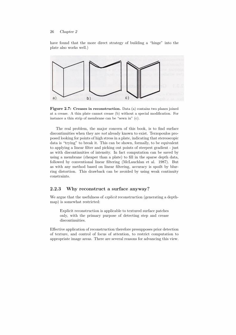
Terzopulos extended Grimson’s method in various ways. The most signif-icant was the impressive improvement in efficiency gained by “multi-grid”techniques (see chapter 6). He also began to consider the effects of sur-face discontinuities on reconstruction. Suppose it were known (somehow),before reconstruction began, that the surface to be reconstructed was notentirely continuous as Grimson supposed, but discontinuous along a cer-tain, known line. The thin plate could be arranged to break along thatline. Similarly if the surface were known to be creased along a certain line,a thin strip of membrane could be sewn into the plate (figure 2.7). (We
26 Chapter 2
have found that the more direct strategy of building a “hinge” into theplate also works well.)
Figure 2.7: Creases in reconstruction. Data (a) contains two planes joined
at a crease. A thin plate cannot crease (b) without a special modification. For
instance a thin strip of membrane can be “sewn in” (c).
The real problem, the major concern of this book, is to find surfacediscontinuities when they are not already known to exist. Terzopoulos pro-posed looking for points of high stress in a plate, indicating that stereoscopicdata is “trying” to break it. This can be shown, formally, to be equivalentto applying a linear filter and picking out points of steepest gradient - justas with discontinuities of intensity. In fact computation can be saved byusing a membrane (cheaper than a plate) to fill in the sparse depth data,followed by conventional linear filtering (McLauchlan et al. 1987). Butas with any method based on linear filtering, accuracy is spoilt by blur-ring distortion. This drawback can be avoided by using weak continuityconstraints.
2.2.3 Why reconstruct a surface anyway?
We argue that the usefulness of explicit reconstruction (generating a depth-map) is somewhat restricted:
Explicit reconstruction is applicable to textured surface patchesonly, with the primary purpose of detecting step and creasediscontinuities.
Effective application of reconstruction therefore presupposes prior detectionof texture, and control of focus of attention, to restrict computation toappropriate image areas. There are several reasons for advancing this view.

Applications of Piecewise Continuous Reconstruction 27
Ambiguity Reconstruction of untextured, smooth surfaces presents a se-vere ambiguity problem. A given circle in space, for instance, could bethe boundary of any one of infinitely many smooth patches (figure 2.8).Grimson/Terzopoulos thin plate reconstruction would plump for a disc.
Figure 2.8: Ambiguity in surface reconstruction.
This dangerously eliminates all the other possibilities - a violation of Marr’sprinciple of “least commitment” (Marr 1982).
In fact the shape of the boundary curve, plus the smoothness constraint,constitute the best available description of the surface patch. There is lit-tle further to be deduced about the shape of the patch. This is nothingto be ashamed of - descriptions of this sort are already a powerful handlefor matching visible surfaces to one another (Pollard et al. 1987) and tostored models (Brooks 1981). New sources of information, such as analysisof surface shading, might add usefully to such descriptions - but that possi-bility must be left for discussion elsewhere (Ikeuchi and Horn 1981, Ikeuchi1983, Blake et al. 1985d). And, of course, if the surface is visibly texturedthe shape ambiguity is resolved by stereoscopic vision, because the textureelements constitute features that can be stereoscopically matched.
Texture masking of monocular features Texture aids stereoscopicvision - but impedes monocular vision. It masks the intensity discontinu-ities generated by surface features (occluding edges etc.). Imagine walkingdown carpeted stairs. The front of each step is an occluding edge, givingrise to a discontinuity in intensity, but mixed up with intensity changes dueto the texture of the carpet. Monocularly, the occluding edge is difficult topick out. (A picture illustrates this shortly). Stereoscopically, however, the

28 Chapter 2
sudden change in depth at the occluding edge, falling off one step onto thenext, is quite unambiguous. (Motion parallax similarly facilitates percep-tion of occluding edges (Longuet-Higgins and Prazdny 1980)).
2.2.4 Surface descriptions
There are two distinct types of usage of information about visible surfaces:reasoning about visible objects, and path planning or collision avoidance.In the first, the goal is to match visible surfaces to one another, or to storedobject-descriptions. The second concerns the “mapping out” of a world inwhich many objects are unknown; it imposes weaker requirements on visualprocessing than the first: it is not necessary to identify the vase on the tableas a precious Chinese porcelain merely to avoid knocking it off. It is enoughto know that it occupies a certain portion of space.
Different descriptions are appropriate in each case. For reasoning aboutobjects, an adequate description might consist of the shapes and positionsof occluding and connect edges and compact descriptions of the shapes ofsmooth patches, together with other features such as colour and texturequality. The cumbersome depth-map has no place here. In this contextit is merely a means to an end, the end of recovering monocularly maskedfeatures.
It is less clear what is the best form of description for path-planningand collision avoidance. A depth-map may be useful for computing thepoint of collision of a given path in space, with the visible surface. Greaterefficiency is achieved, though, if the visible surface can be “protected” by abounding polygon, computed directly from sparse depths (Boissonat 1984),without the use of an intermediate depth map.
The point is that direct applications for depth maps, as descriptions ofvisible surfaces, are at best limited and at worst, perhaps, non-existent.
2.2.5 Localising discontinuities
Incorporation of discontinuities into the reconstructed surface by means ofweak continuity constraints was originally suggested in (Blake 1983a). Suchideas have recently been developed from (Geman and Geman 1984) by Mar-roquin (1984). Alternative approaches have been suggested by Grimson andPavlidis (1985) and Terzopoulos (1985). The special problems presented bythe fact that stereoscopic data is sparse are discussed fully in chapters 4and 7.
Fitting a weak membrane to sparse depth data is illustrated in figure2.9, and for a real image in figures 2.10 and 2.11.

Applications of Piecewise Continuous Reconstruction 29
Figure 2.9: Fitting a membrane to sparse depth data. Artificially gener-
ated, sparse depth data (a) in which displayed grey-level encodes depth, contains
a sequence of layers, like a wedding cake viewed from above. After fitting with a
weak membrane, the piecewise continuous surface is recovered (b), together with
discontinuities between layers.
A weak membrane is sufficient for labelling occluding edges only; theyappear as tears in the membrane. To detect connect edges as well, a thinplate must be used, capable both of tearing and of buckling. An exampleof the application of a weak plate to stereoscopic images is given in figure2.12.
2.3 Surface reconstruction from dense rangedata
Optical range-finders produce raw arrays of depth values. These requireorganisation before they are usable for path-planning and collision avoid-ance, or for matching to object models. It is desirable to make explicit thediscontinuities in depth and its derivative; they correspond to occlusionsand creases between surfaces in the scene. This is quite like the problem ofdetecting discontinuities of intensity. But, in addition, invariance to changeof viewpoint (Blake 1984) must be ensured, in order to maintain stabilityunder viewer motion. This would be of crucial importance in a real timesystem, but is important even for analysis of single frames, if surface de-scriptions are to be robust.
Figure 2.13 shows the results of fitting a plate to laser rangefinder data,under weak continuity constraints. A weak plate is used (rather than a weak

30 Chapter 2
Figure 2.10: Weak membrane reconstruction of real stereo data. A
stereo pair (a) of a foam block, with a step discontinuity across the middle, that
is all but invisible monocularly. Stereo correspondence using a state-of-the-art
matching algorithm (Pollard et al. 1985) produces depths along sparse contours
(b). The reconstructed surface is shown with its contour of discontinuity (c).

Applications of Piecewise Continuous Reconstruction 31
Figure 2.11: Isometric plots of the stereoscopic data from figure 2.10b and the
reconstructed surface in figure 2.10c.

32 Chapter 2
Figure 2.12: Applying a weak plate to sparse, stereoscopic depths.
(a) Stereo image-pair. (b) Stereoscopically matched features. Both steps and
creases are recovered by the plate (c), shown superimposed on the reconstructed,
dense depth-map. Creases are marked as thin white lines, whilst steps are marked
as thick, black lines. A few spurious creases have been generated as a result of
“ghost” matches in the stereoscopically viewed texture.

Applications of Piecewise Continuous Reconstruction 33
Figure 2.13: Fitting a weak plate to a laser rangefinder depth-map.
The depth map (a) is of a telephone handset. Both steps and creases are recovered
by the plate (b), giving a piecewise smooth approximation to the data. (Creases
are marked as white lines, whilst steps are marked as black lines.)
membrane) so that both step and crease discontinuities can be recovered.
2.4 Curve description
At an early stage of visual processing, descriptions of the shape and connec-tivity of curves are needed. For example, connect and occluding edges, ob-tained by surface reconstruction, are unorganised. They are simply chainsof points arranged on a grid. The chains must be aggregated to form com-pact, stable descriptions, consisting of the positions of corners, junctionsand curve endings, together with the approximate shape of smooth curvesegments.
Discontinuities again have a primary role. Commonly, a curve is con-verted to tangent angle/arc-length (θ, s) form, and filtered to detect cor-ners (step discontinuities in θ) and possibly also curvature discontinuities(Perkins 1978, Asada and Brady 1986, Ramer 1975, Zucker et al. 1977,Zucker 1982, Blake et al. 1986a). This may be done at a variety of spatialscales in order to obtain both coarse and fine views of the curve’s shape.Corners, for instance, appear as step discontinuities in tangent angle θ.Sharp corners look discontinuous at all scales, but rounded ones only atcoarse scale. Just as with discontinuities in intensity and in visible surfaces,discontinuities in tangent angle can be detected by linear filtering, followedby labelling of gradient maxima. But again, blurring distortion causes lo-calisation errors which are avoided when weak continuity constraints are

34 Chapter 2
used instead.In figure 2.14 a simple hand drawn curve is shown. Corners have been
detected by fitting a weak elastic string to the (θ, s) data. Results at a vari-ety of scales are plotted in “scale-space” (figure 2.14d). Note the remarkablyuniform structure of the scale-space - this agrees with theoretical predic-tions. Uniformity has the advantage that tracking features in scale-spacebecomes trivial. Tracking is essential to maintain correct correspondencebetween features at coarse and fine scales. But under linear filters such asthe gaussian and its derivatives, complex structure arises, which is difficultto track and harder still to interpret (Asada and Brady 1986, Witkin 1983).A weak string scale-space for a silhouette taken from a real image, is shown
Figure 2.14: Scale-space filtering. The hand drawn curve (a) segmented
at coarse scale (b) and reconstructed by fitting arcs between discontinuities (c).
When weak elastic strings are fitted at a variety of spatial scales, the disconti-
nuities trace out a uniform “fingerprint” (straight vertical lines) in “scale-space”
(d). Notice that, as expected, the fingerprint of the small notch on the curve
appears only at small scales; the rounded corner’s fingerprint appears only at
large scales.

Applications of Piecewise Continuous Reconstruction 35
in figure 2.15.The weak string curve filter, in addition to running on clean, isolated
curves as in figures 2.14, 2.15, can also operate on edges embedded in animage. This is shown in figures 2.16 and 2.17. A simple linear filter runsalong the edges, estimating local tangent angles. The weak string is thenapplied to the “graph” of edges, just as they are, embedded in the image.Corners show up as discontinuities of tangent angle as before. In addition,T-junctions generate 3-way discontinuities (continuous tangent angle alongthe crossbar, but discontinuous at the top of the downstroke). At a Y-junction, tangent angles on all 3 arms are discontinuous.

36 Chapter 2
Figure 2.15: Weak string scale-space applied to a real image. Sillhou-
ette (a) segmented at coarse scale (b) and reconstructed by fitting arcs between
discontinuities (c). It is apparent that discontinuities and arcs together constitute
a compact but accurate representation of the silhouette. (d) Scale-space. Most
features, in this case, are visible at both coarse and fine scale, except for the
curved base of the handle, visible at coarse scale only. (Data after Asada and
Brady (1986).)

Applications of Piecewise Continuous Reconstruction 37
Figure 2.16: Corner and junction detection: synthesised image. Dark
blobs mark discontinuities in tangent angle, obtained from fitting weak strings to
the entire “graph” of edges.
Figure 2.17: Corner and junction detection: real image.

38 Chapter 2

Chapter 3
Introduction to WeakContinuity Constraints
For illustrative purposes, consider the simplest weak continuity problem:detection of step discontinuities (edges) in 1D data. The aim is to constructa piecewise smooth 1D function u(x) which is a good fit to some data d(x).This is achieved by modelling u(x) as a “weak elastic string” - an elasticstring under weak continuity constraints. Discontinuities are places wherethe continuity constraint on u(x) is violated. They can be visualised asbreaks in the string. The weak elastic string is specified by its associatedenergy; the problem of finding u(x) is then the problem of minimising thatenergy.
3.1 Detecting step discontinuities in 1D
The behaviour of the elastic string over an interval x ∈ [0, N ] is defined byan energy, which is a sum of three components:
P : the sum of penalties α levied for each break (discontinuity) in thestring.
D: a measure of faithfulness to data.
D =∫ N
0
(u− d)2dx

40 Chapter 3
S: a measure of how severely the function u(x) is deformed.
S = λ2
∫ N
0
u′2dx.
This is the elastic energy of the string itself, that is stored when the stringis stretched. The constant λ2 is a measure of elasticity or “stretchability”or willingness to deform1.
The problem is to minimise the total energy:
E = D + S + P (3.1)
- that is, for a given d(x), to find that function u(x) for which the totalenergy E is smallest. Without the term P (if the energy were simply E =D+S) this problem could be simply solved using the calculus of variations.For example fig 3.1c shows the function u that minimises D+ S, given thedata d(x) in fig 3.1a. It is clearly a compromise between minimising D andminimising S - a trade-off between sticking close to the data and avoidingvery steep gradients. The precise balance of these 2 elements is controlledby λ. If λ is small, D (faithfulness to data) dominates. The resulting u(x)is a close fit to the data d(x). In fact, λ has the dimensions of length, andit will be shown that it is a characteristic length or scale for the fittingprocess.
When the P term is included in E, the minimisation problem becomesmore interesting. No longer is the minimisation of E straightforward math-ematically. E may have many local minima. For example, for the problemof fig 3.1, b) and c) are both local minima. Only one is a global minimum;which one that is depends on the values of α, λ and the height h of the stepin a). If the global minimum is b) then the reconstruction u(x) contains adiscontinuity; otherwise, if it is c), u(x) is continuous.
3.2 The computational problem
The “finite element method” (Strang and Fix 1973) is a good means of con-verting continuous problems, like the one just described, into discrete prob-lems. In the case of the string it is relatively easy. The continuous interval[0, N ] is divided into N unit sub-intervals (“elements”) [0, 1], ..., [N − 1, N ],and nodal values are defined: ui = u(i), i = 0...N . Then u(x) is representedby a linear piece in each sub-interval (fig 3.2). The energies defined earlier
1Really, interpreting S as a stretching energy is only valid when the string is approx-imately aligned with the x axis. Another way to think of S is that it tries to keep thefunction u(x) as flat as possible.

Introduction to Weak Continuity Constraints 41
Figure 3.1: Calculating energy for data consisting of a single step. (a)
Data. (b) A reconstruction with one discontinuity. (c) A continuous reconstruc-
tion.

42 Chapter 3
Figure 3.2: Dividing a line into sub-intervals or “elements”.
now become:
D =N∑0
(ui − di)2 (3.2)
S = λ2N∑1
(ui − ui−1)2(1− li) (3.3)
P = α
N∑1
li (3.4)
where li is a so-called “line-process”. It is defined such that each li is aboolean-valued variable.
Either: li = 1 indicating that there is a discontinuity in the sub-intervalx ∈ [i− 1, i].
or: li = 0 indicating continuity in that subinterval - ui, ui−1 are joined bya spring.
Note that when li = 1 the elastic string is “broken” between nodesi− 1 and i and the relevant energy term in (3.3) is disabled. (Geman andGeman (1984) coined the term “line-process” as a set of discrete variablesdescribing edges in 2D; here we have a simple case, appropriate in 1D.)

Introduction to Weak Continuity Constraints 43
3.3 Eliminating the line process
The problem, now in discrete form, is simply:
min{ui,li}
E.
It transpires that the minimisation over the {li} can be done “in advance”.The problem reduces simply to a minimisation over the {ui}. Exactly howthis is achieved will be explained in chapter 6. The reduced problem ismore convenient for two reasons:
• The computation is simpler as it involves just one set of real variables{ui}, without the boolean variables {li}.
• The absence of boolean variables enables the “graduated non-convexityalgorithm”, described later, to be applied.
It will be shown that once the line-process {li} has been eliminated, theproblem becomes
min{ui}
F , where F = D +N∑1
g(ui − ui−1). (3.5)
The neighbour interaction function g will be defined precisely in chapter 6but to give some idea of how it acts, it is plotted in figure 3.3. The termS + P in (3.1) has been replaced by the
∑g(..) term in (3.5). Note that
nothing of value has been thrown away by eliminating line variables. Theycan very simply be explicitly recovered from the optimal {ui} (this is alsoexplained in chapter 6).
3.4 Convexity
The discrete problem has been set up. The task now is to minimise thefunction F ; but that proves difficult, for quite fundamental reasons. Func-tion F lacks the mathematical property of “convexity”. What this means isthat the system ui may have numerous stable states, each corresponding toa local minimum of energy F . Such a state is stable to small perturbations- give it a small push and it springs back - but a large perturbation maycause it to flip suddenly into a state with lower energy.
There may be very many local minima in a given F . In fact there is(in general) one local minimum of F corresponding to each state of the lineprocess li - 2N local minima in all! The goal of the weak string computationis to find the global minimum of F ; this is the local minimum with the lowest

44 Chapter 3
Figure 3.3: Energy of interaction between neighbours in the weak
string. The central dip encourages continuity by pulling the difference ui−ui−1
between neighbouring values towards zero. The plateaus allow discontinuity: the
pull towards zero difference is released, and the weak continuity constraint has
been broken.
energy. Clearly it is infeasible to look at all the local minima and comparetheir energies.
How do these local minima arise? The function F can be regarded as theenergy of a system of springs, as illustrated in figure 3.4a. We will see that,like the magnetic dipole system in chapter 1, it has many stable states.Vertical springs are attached at one end to anchor points, representingdata di which are fixed, and to nodes ui at the other end. These springsrepresent the D term in the energy F (3.5). There are also lateral springsbetween nodes. Now if these springs were just ordinary springs there wouldbe no convexity problem. There would be just one stable state: no matterhow much the system were perturbed, it would always spring back to theconfiguration in figure 3.4a. But in fact the springs are special; they are theones that enforce weak continuity constraints. Each is initially elastic but,when stretched too far, gives way and breaks, as specified by the energyg in figure 3.3. As a consequence, a second stable state is possible (figure3.4b) in which the central spring is broken. In an intermediate state (figure3.4c) the energy will be higher than in either of the stable states, so thattraversing from one stable state to the other, the energy must change as infigure 3.4d. For simplicity, only 2 stable states have been illustrated, butin general each lateral spring may either be broken or not, generating theplethora of stable states mentioned above.
No local descent algorithm will suffice to find the minimum of F . Localdescent tends to stick, like the fly shown in figure 3.4, in a local minimum,

Introduction to Weak Continuity Constraints 45
Figure 3.4: Non-convexity: the weak string is like a system of conventional
vertical springs with “breakable” lateral springs as shown. The states (a) and
(b) are both stable, but the intermediate state (c) has higher energy than either
(a) or (b). Suppose the lowest energy state is (b). A myopic fly with vertigo,
crawling along the energy transition diagram (d) thinks state (a) is best - he has
no way of seeing that, over the hump, he could get to a lower state (b).

46 Chapter 3
and there could be as many as 2N local minima to get stuck in. Somehowsome global “lookahead” must be incorporated. The next section explainshow the Graduated Non-Convexity (GNC) algorithm does this.
3.5 Graduated non-convexity
A method of minimising F is needed which avoids the pitfall of sticking inlocal minima. Stochastic methods such as “Simulated Annealing” (Kirk-patrick et al. 1982) avoid local minima by random fluctuations, spasmodicinjections of energy, to shake free of them (figure 3.5a). Although thisguarantees to find the global minimum eventually, the amount of compu-tation required may be very large (Geman and Geman 1984). It would
Figure 3.5: a) Stochastic methods avoid local minima by using random motions
to jump out of them. b) The GNC method constructs an approximating convex
function, free of spurious local minima.

Introduction to Weak Continuity Constraints 47
appear, however, to be in the interests of computational efficiency to use anon-random method. GNC, rather than injecting energy randomly, uses amodified cost function (fig 3.5b).
In the GNC method, the cost function F is first approximated by a newfunction F ∗ which is convex and hence can only have one local minimum,which must also be a global minimum2. Descent on F ∗ (descending, thatis, in the (N +1)-dimensional space of variables {ui}) must land up at thatminimum. Now, for certain data di this minimum may also be a globalminimum of F - which is what we were after. There is a simple test todetect whether or not this has succeeded (fig 3.6a,b). In fact (see chapter7) success is most likely when the scale parameter λ is small.
A more general strategy, that works for small or large λ, is to use awhole sequence of cost functions F (p), for 1 ≥ p ≥ 0. These are chosenso that F (0) = F , the true cost function, and F (1) = F ∗, the convexapproximation to F . In between, F (p) changes, in a continuous fashion,between F (1) and F (0). The GNC algorithm is then to optimise a wholesequence of F (p), for example {F (1), F (1/2), F (1/4), F (1/8), F (1/16), F (1/32)},one after the other, using the result of one optimisation as the startingpoint for the next. As an example, optimisation of a non-convex F , using asequence of just 3 functions, is illustrated in fig 3.6c. Initially, optimisationof F (1) ≡ F ∗ produces u∗ but (let us suppose) this happened not to be theglobal optimum of F . (Note that any starting point will do for optimisingF (1). That is because F (1), being convex, has only one minimum, which willbe attained by descent, regardless of where descent starts.) But successiveoptimisation of F (p) as p decreases “pulls” towards the true global optimumof F . Exactly how the functions F (p) are constructed must be left untillater. It all depends on making F ∗ a good convex approximation to F .Suffice it to say that, like F in (3.5), F ∗ and all the F (p) are sums of localfunctions:
F (p) = D +N∑1
g(p)(ui − ui−1), (3.6)
and this is important when it comes to considering optimisation algorithms.Of course, the trick is to choose the right neighbour interaction functiong(p). This is all explained at some length in chapter 7.
There are numerous ways to minimise each F (p), including direct descentand gradient methods. Direct descent is particularly straightforward toimplement and runs like this: propose a change in one of the nodal valuesui, see if that leads to a reduction in F (p) (this only involves a localcomputation); if it does then make the change. A simple program which
2Actually there are some details to take care of here, distinguishing between convexityand strict convexity.

48 Chapter 3
Figure 3.6: The minimum of a non-convex function F may be found by min-
imising a convex approximation F ∗ (a). If that does not work (b), the minimum
may still be found by the GNC algorithm, which runs downhill on each of a
sequence of functions (c), to reach the true global optimum.

Introduction to Weak Continuity Constraints 49
implements GNC by direct descent is outlined in fig 3.7. It can be made to
for p ∈ {1, 1/2, 1/4, 1/8, 1/16, 1/32} dofor δ := 1; δ ≥ δmin; δ := δ/2 dochanged := truewhile changed dochanged := falsefor i = 0...N doif F (p)(u1, .., ui + δ, .., uN ) < F (p)(u1, .., ui, .., uN ) thenui := ui + δchanged := true
else if F (p)(u1, .., ui − δ, .., uN ) < F (p)(u1, .., ui, .., uN ) thenui := ui − δchanged := true
Figure 3.7: A direct descent algorithm for GNC - see text for details
run quite satisfactorily with fixed point arithmetic. As F (p) is expressedas a sum over i = 0, ..., N of local terms (3.6), the effect of altering aparticular ui (tested in the if and else if statements) can be computed fromjust a few of those terms. For example ui appears only in g(p)(ui − ui−1),g(p)(ui+1 − ui) and, in D, in the term (ui − di)2. Not only does thissimplify the computation of the effect on F (p) of changing ui, but it isalso possible to perform such computations on many ui in parallel. Moreefficient algorithms, based on gradient descent methods, are described inchapter 7.
Figure 3.8 shows the GNC method in operation, solving the 1D weakelastic string problem. The successive gradient descent scheme (SOR) ofchapter 7 is used. For small values of the scale parameter λ the total timefor execution3 is about 0.001N seconds, where N is the length of the datavector. This works out at about 50 arithmetic operations per data element.
3On a SUN2 computer, with SKY floating point board

50 Chapter 3
Figure 3.8: Snapshots of GNC: Initial data as in figure 2.2 on page 19. As
GNC progresses, parameter p is decreased. (The significance of parameters h0
and c is explained in subsequent chapters.)

Chapter 4
Properties of the WeakString and Membrane
The previous chapter introduced the weak string as a 1D discontinuitydetecting filter. This chapter examines both it and its 2D equivalent, theweak membrane, as variational problems. Recall that the energy of theweak string is described by the function
E = D + S + P (4.1)
=∫
(u(x)− d(x))2 dx+ λ2
∫u′2(x) dx+ αZ (4.2)
where α and λ are constants - parameters of the system - and integrationis between suitable limits. The first two terms D,S specify the behaviourof each continuous section of the piecewise elastic string u(x), attachedby “springs” to the data d(x). The last term is a measure of the set ofdiscontinuities in u(x); Z is taken to be simply the total number of pointsx at which u(x) is discontinuous. In 1D, this definition of Z is more or lessthe only sensible one. It will be seen that, in 2D, with the membrane, thereis more than one reasonable way of defining Z.
So far it has appeared that constants α, λ are arbitrary parameters; itis not clear how they should be fixed. But variational analysis of the weakstring’s behaviour with certain specially chosen data d(x) allows extremalenergy E to be predicted, as a function of α, λ. This can be done both forcontinuous u and when u includes one or more discontinuities. The weakstring/membrane will adopt the lowest energy configuration. So comparisonof energies, with and without discontinuities, determines exactly what effectλ and α have on the detection of discontinuities. Most of our results (butnot their derivations) were reported in (Blake and Zisserman 1985a, 1986b).

52 Chapter 4
The principal conclusions of this chapter are that
• The parameter λ is a characteristic length or scale (figure 4.1).
• The ratio h0 =√
2α/λ is a “contrast” sensitivity threshold, determin-ing the minimum contrast for detection of an isolated step edge. Astep edge in the data counts as isolated if there are no features withinλ of it - and this property itself reinforces the interpretation of λ as acharacteristic length. In addition to being a characteristic length forsmoothing continuous portions of the data, λ is also a characteristicdistance for interaction between discontinuities.
• When two similar steps in the data are only a apart (a � λ) theyinteract as follows: the threshold for detection (labelling the steps asdiscontinuities) is increased by a factor
√λ/a, compared with the con-
trast threshold for an isolated step. This constitutes a proof that theweak string is not equivalent to any linear operator followed by thresh-olding, for which the corresponding factor would be proportional to1/a, not 1/
√a. It is complementary to the finding of Mumford and
Shah (1985) that the weak string does behave like a linear operatorwith thresholding, but only for isolated, non-interacting discontinu-ities. Such distinctive, non-linear behaviour is a property also of themembrane, with interacting discontinuities in 2D.
• The ratio gl = h0/2λ is a limit on gradient, above which spuriousdiscontinuities may be generated. This property is inferred from be-haviour when fitting data in the form of a ramp: if the gradientexceeds gl one or more discontinuities may appear in the fitted func-tion.
• It can be shown that, in a precise sense, localisation accuracy (forgiven signal-to-noise) is high. In fact it is qualitatively as good as the“difference of boxes” operator - but without any false zero-crossingsproblem (see (Canny 1983)). Non-random localisation error is alsominimised. Given asymmetrical data, gaussians and other smoothlinear operators make consistent errors in localisation. The weakstring, based as it is on least squares fitting, does not.
• The parameter α is a measure of immunity to noise. If the mean noisehas standard deviation σ, then no spurious discontinuities are gener-ated provided α > 2σ2, approximately. This theoretical predictionis borne out in the computer implementation (e.g. figure 4.2).
• The membrane has a hysteresis property - a tendency to form unbro-ken edges. This is an intrinsic property of membrane elasticity, and

Properties of the Weak String and Membrane 53
Figure 4.1: Weak membrane edge detector: the effect of varying scale (λ)
and contrast sensitivity is shown. (Data d(x, y) was approximately the logarithm
of image intensity. The image is 128 pixels square.)

54 Chapter 4
Figure 4.2: A light square on a dark background, with added noise (a). Sig-
nal-to-noise ratio is 1. A weak membrane is well able to reconstruct the signal
(b). (c) Labelled discontinuities. (α/σ2 ≈ 4.)

Properties of the Weak String and Membrane 55
happens without any need to impose additional cost on edge termina-tions.
• The weak string or membrane can be used with sparse data. Thedensity of stereo depth data (depths obtained from matching a stereo-scopic image pair) is limited by the density of strongly localised fea-tures in images. Also hyperacuity - sub-pixel localisation of discon-tinuities - can be implemented by forming a fine grid on which thedata (intensity or depth) is distributed sparsely.
• Finally the weak string/membrane is quite unable to label crease dis-continuities. This is because a membrane conforms quite happily to acrease without any associated energy increase. The weak plate, how-ever, can be used to detect creases. This is because it has a 2nd orderenergy (a function of 2nd derivatives) unlike the membrane energywhich is 1st order; but that must be left until the next chapter.
4.1 The weak string
4.1.1 Energy of a continuous piece
Suppose the positions of all discontinuities were given in advance. Thenthe energy of each continuous piece of u could be computed separately.One way of doing this1 is to construct the solution u(x), in each piece, byconvolving d with a Green’s function G:
u(x) =∫G(x, x′)d(x′) dx′ (4.3)
where, in the case of a bi-infinite interval,
G(x, x′) =12λe−|x−x′|/λ (4.4)
which is plotted in figure 4.3. The characteristic length or scale of the filteris simply the parameter λ. In the case of a finite interval, the filter shapeis similar, but modified near interval boundaries (see appendix A). Havingobtained u(x) the energy is (appendix A)
E =∫ ∞
−∞d(x)(d(x)− u(x)) dx. (4.5)
This can be used to compute energies for various forms of data d(x).1An alternative Fourier method is given in appendix A.

56 Chapter 4
Figure 4.3: Green’s function for the string. The elastic string has the
effect of smoothing data d with the filter shown.
4.1.2 Applying continuity constraints
The behaviour of the weak string depends on the size of the energy increasewhen a discontinuity is removed so that u(x) is forced to be continuousacross an interval boundary. A closely related question is: how much doesthe energy of the string, in some interval, increase when the position of oneend is fixed? The answers to both questions, remarkably, turn out to bevirtually independent of the precise form of the data d. They will thereforebe satisfyingly general.
Suppose the string u(x), x ∈ [0, L] is fixed at one end, so that u(0) = z(figure 4.4a). Its energy is (appendix A):
E = E(z − z)2 + E0 (4.6)
where E0, z are values of E, z when the string is unconstrained and E is aconstant depending only on L, λ - quite independent of the data:
E = λ tanh(L
λ
)(4.7)
≈ λ when L� λ. (4.8)
As expected, energy E is smallest in the “resting” position z = z, u = u,and increases quadratically as z is displaced.
When u is forced to be continuous at the join of two intervals, u iseffectively fixed, at the ends of both intervals, to the common value z thatminimizes the total increase in energy (figure 4.4b). It is easily shown

Properties of the Weak String and Membrane 57
Figure 4.4: Fixing one end of a string increases its energy (a). Enforcing
continuity fixes ends of two strings to some common value (b).

58 Chapter 4
(appendix A) that this total increase in energy is
∆E = h2
(1E1
+1E2
)−1
, (4.9)
where h = |z2 − z1| - the “effective” step height.If both intervals have lengths L1, L2 � λ, then, from (4.8), E1 = E2 = λ
and the energy increase is just
∆E =12h2λ. (4.10)
4.1.3 Sensitivity to an isolated step
The simplest possible data comprises a single isolated step discontinuity asin figure 4.4b. The lowest energy solution contains a discontinuity at thestep if and only if the energy increase ∆E−α on removing the discontinuitysatisfies ∆E − α > 0. (Remember, from chapter 3, that the α term repre-sents the energy penalty for one discontinuity.) From (4.10) the conditionis met when
h > h0 =
√2αλ. (4.11)
So the existence of an isolated discontinuity in weak string reconstructionu of data d, at a particular point, depends entirely on whether the effectivestep height h exceeds the threshold h0. It can also be shown that
∆E = 2λ3 (u′(0))2 , (4.12)
(where u(x) is now the continuous reconstruction of d(x)) so an equivalentcondition is that
u′(0) >h0
2λ. (4.13)
Of course it has been assumed so far that only one possible site forthe discontinuity is under consideration. The question of exactly wherediscontinuities choose to form has not been answered - it will be dealt withlater in the chapter. Detection of a discontinuity appears, so far, to dependon a remarkably simple threshold rule. In fact that is true only for isolatedsites. When two sites for discontinuities come within interaction range (λ)behaviour is somewhat modified.
4.1.4 Interaction of adjacent steps
A top hat (figure 4.5a) consists of two steps back to back. The energy of a
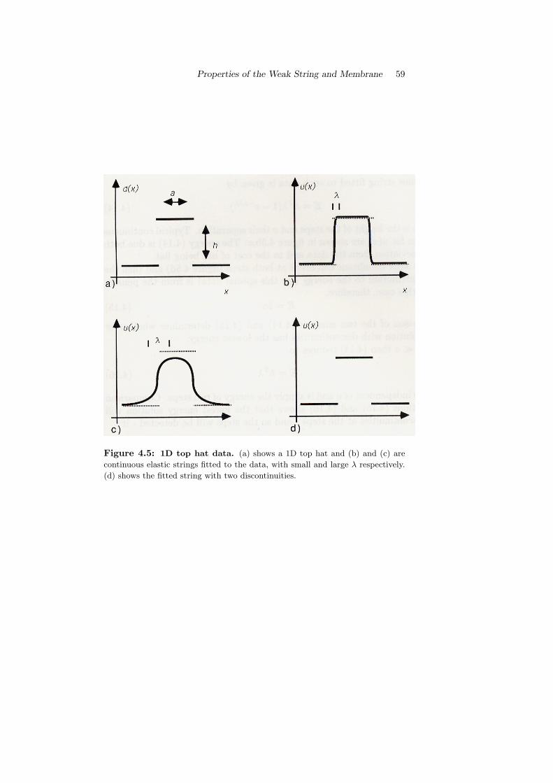
Properties of the Weak String and Membrane 59
Figure 4.5: 1D top hat data. (a) shows a 1D top hat and (b) and (c) are
continuous elastic strings fitted to the data, with small and large λ respectively.
(d) shows the fitted string with two discontinuities.

60 Chapter 4
continuous string fitted to such data is given by
E = h2λ(1− e−a/λ) (4.14)
where h is the height of the steps and a their separation. Typical continuoussolutions for u(x) are shown in figure 4.5b,c. The energy (4.14) is due bothto the deviation from the data and to the cost of not being flat.
The weak membrane can break at both steps (figure 4.5d) and then theonly contribution to the energy (for this special data) is from the penalty2α. In this case, therefore,
E = 2α. (4.15)
Comparison of the two energies (4.14) and (4.15) determines whether ornot a solution with discontinuities has the lowest energy.
If λ� a then (4.14) reduces to
E = h2λ (4.16)
which is independent of a and is simply the energy of two steps. Comparisonof equations (4.15) and (4.16) shows that the lowest energy solution willhave discontinuities at the steps - and so the steps will be detected - if
h > h0 =
√2αλ
This is the same as the threshold for a single step (4.11). Consequently, ifthe step separation is large compared to λ then the steps do not interferewith each other - they are treated independently by the weak string.
If the steps are close to each other (a� λ) the energy (4.14) is reducedand the steps interfere. The energy in that case is
E = h2a, (4.17)
independent of λ. Comparing this with the penalty 2α, the discontinuoussolution (with 2 steps) has lower energy if h > h0
√λ/a. The contrast
threshold is increased by a factor√λ/a, compared with that for isolated
steps.The interference effect extends the interpretation of λ, already estab-
lished by the form of the Green’s function, as a scale parameter. If dis-continuities are separated by distances which are large compared to λ thenthey do not interfere with each other and are considered independently bythe system.
Although this result has been obtained for an ideal top hat it can begeneralised just as threshold behaviour for an isolated discontinuity applied,

Properties of the Weak String and Membrane 61
not only for an ideal step, but also for general data (figure 4.4b). The gen-eralisation of the top hat would include any pair of discontinuities with thesame effective step height. It is possible to generalise still further (appendixA, equation (A.23)) to cover any pair of interacting discontinuities. In thatcase it is possible that both, one or neither discontinuities may be detected.For example, in the case that the spacing between discontinuities satisfiesa � λ, so that the interaction is strongest, the number of discontinuitiesdetected depends on which of the following energies is least: none : if 1
2λ(h1 − h2)2 + ah1h2 is leastone : if ah2
1 + α is leasttwo : if 2α is least
(4.18)
where h2, h1 are effective step heights with h2 > h1 (figure 4.6).
Figure 4.6: Interaction of a pair of step discontinuities (see text).
Double steps generated by digitisation: A particular case of inter-est are spurious steps (figure 4.7) which occur frequently in digitised data.(Discrete analysis should really be used here, but in fact it makes littledifference to the outcome.) Comparing energies with one (central) discon-tinuity, which can be shown to be
E = α+14h2a
and with two discontinuitiesE = 2α,
the undesirable effect is eliminated provided
h
h0<
√2λa. (4.19)

62 Chapter 4
Figure 4.7: Double edges can occur on gradients caused by digitisation effects.
They are suppressed by using a sufficiently large scale parameter λ.
The larger λ is, the larger the step height h can be, before a double edgeoccurs.
4.1.5 The gradient limit
Data in the form of a ramp of finite extent is shown in figure 4.8a. As beforethe energy of the continuous solution (figure 4.8b) is compared with thatof a solution with a single discontinuity (figure 4.8c). The minimum energysolution with one step discontinuity has its step placed symmetrically atthe centre of the ramp. The energies for the two cases are
E = g2λ2(a− λ(1− e−a/λ)) (4.20)
for the continuous membrane and, with a single step discontinuity,
E = α+ g2λ2(a− 2λe−a2λ (2 cosh
a
2λ− 2 + sinh
a
2λ)) (4.21)
where a is the extent of the ramp, h its height and g its gradient (g = h/a).Again, consider the limits of large and small λ relative to a. If λ � a
then the ramp looks (at a scale of λ) like a step. As expected, the contrastthreshold h > h0 applies.
If λ� a then a step is detected if
g > gl =√
α
2λ3=h0
2λ. (4.22)

Properties of the Weak String and Membrane 63
Figure 4.8: 1D finite ramp data (a) with continuous string fitted to it (b). (c)
shows the lowest energy solution with a single discontinuity.
This is the “gradient limit” effect: if the gradient of a ramp exceeds thelimit, a discontinuity appears in its reconstruction. And if g is much greaterthan gl then a solution with multiple breaks might have smallest energy.This is a fundamental limitation of the weak string/membrane - a steepramp with large extent (relative to λ) will be detected as a multiple step.The rod/plate (chapter 5) does not have this disadvantage.
Performance of the weak string and membrane, as characterised by vari-ational analysis so far, is summarised in figure 4.9.
4.2 Localisation and spurious response innoise
4.2.1 Localisation in scale space: uniformity property
The introductory discussion of the applications of weak continuity includeda brief reference to the task of curve description. A variation on Asada andBrady’s use of gaussian scale-space filtering (Asada and Brady 1986)

64 Chapter 4
Figure 4.9: Summary of the performance of a weak string/membrane.

Properties of the Weak String and Membrane 65
employs a weak string as the filter (Blake et al. 1986a). Typical results weredisplayed in figure 2.14 on page 34. Its most interesting property is that ofuniformity; lines in the scale space diagram (figure 2.14d) are vertical. Thatis a graphical representation of the fact that the positions of discontinuitiesdo not vary as the filter scale λ varies. Localisation across scale is veryaccurate. This is in distinct contrast to the behaviour of scale-space undera gaussian (or other smooth) linear filter. If an asymmetric signal d(x)is filtered (figure 4.10a) there is a systematic error in localisation of thediscontinuity (Asada and Brady 1986) which is proportional to the filterscale w.
Figure 4.10: An asymmetric step (a) filtered by a gaussian filter of scale w
generates a gradient maximum which can be used to mark the discontinuity (b).
But the mark has an error of localisation which increases with w, as shown in the
scale space diagram (c).
Such error can, in principle, be removed by tracking from coarse scale,where noise is well suppressed, to fine scale, where localisation is good. Inpractice it is possible only to sample scale-space at a few discrete scales,so that correct tracking becomes a difficult problem (figure 4.11). No suchproblem occurs under weak continuity constraints because of uniformity -tracking is trivial. Indeed, the weak string does not demand an entire scalespace at all, in the sense that Gaussian filtering does. One or two scalesλ may suffice for the purposes of interpretation - a fine and a coarse viewperhaps. The examples given in chapter 2 (figures 2.14 and 2.15) neededonly a single scale to achieve an accurate reconstruction.

66 Chapter 4
Figure 4.11: Tracking a sampled Gaussian scale-space. In principle,
fingerprints can be tracked from coarse to fine scale (a). In practice, sampling
makes this a much more difficult task (b).
When a similar asymmetric step is filtered by a weak string, the discon-tinuity in the string remains precisely on the step, regardless of the scaleparameter λ in the string energy. That is the underlying reason for theuniformity property. Intuitively this is made clear in figure 4.12.
The intuitive argument can be made more precise. This is done in twodifferent ways. First the now familiar variational approach is used to derivethe energy E(ε) of the weak string, as a function of discontinuity location ε,for the data in figure 4.10. The global minimum is shown to exist stably atε = 0, having a V-shaped profile as in figure 4.12c, regardless of λ. Second,variational results show that the discontinuity in the string clings to ε = 0even in the presence of small variations in d(x) near the step.
The effect of the weak string on the asymmetric step is analysed bymeans of (A.15) and (A.16) of appendix A, which gives the energy of acontinuous string stretched over a step/ramp as in figure 4.10. The energyE(ε) for the asymmetric step of figure 4.12 can be shown to have the form
E(ε) =
const. − 12 (h− gλ)2λ exp
(−2|ε|
λ
)for ε < 0
const. − 12 (h+ gλ)2λ exp
(−2|ε|
λ
)for ε > 0
. (4.23)
(This assumes that λ is much less than the total extent of data d(x) oneither side of the step.) Energy E(ε) is clearly monotonic increasing with|ε| so that the global minimum is at ε = 0. Curious degenerate cases occurwhen h = ±gλ, and the stability of the global minimum is lost. To first

Properties of the Weak String and Membrane 67
Figure 4.12: Localisation of the weak string: consider a weak string fitted
to data d(x) containing a step, but with its discontinuity displaced ε from the
step (a) or (b). The hatched “error area” is roughly a rectangle h × ε, and so
generates a square error contribution to the energy of approximately h2|ε|. The
minimum energy is clearly at ε = 0 (c).
order in |ε| the energy is
E(ε) = E(0) +{
(h− gλ)2|ε| for ε < 0(h+ gλ)2|ε| for ε > 0. (4.24)
This means that locally, around ε = 0, the V-shape of the minimum (figure4.12c) is preserved, albeit somewhat skewed. This holds for any λ (whichis not too large and avoids the degeneracies just mentioned) so that preciselocalisation is maintained right across scale space (figure 4.12c).
Mumford and Shah (1985) derive an extremality condition which is nec-essary for the existence of a global minimum of energy E(ε). It assumesthat the discontinuity at x = ε is isolated (on the scale of λ). The condition,in our notation, is that
u′′c (ε) = 0 (4.25)
where uc(x) is the configuration of a continuous string fitted to the datad(x). This is directly related to the earlier result (4.12) which, applied here,shows that the energy gain on allowing a discontinuity at x = ε is
2λ3 (u′c(ε))2.
Equation (4.25) is therefore simply a necessary condition for maximisingthat energy gain. But since, from the Euler-Lagrange equation (A.2), u′′c =

68 Chapter 4
λ−2(uc − d) the condition (4.25) can be re-expressed as
uc(ε) = d(ε) (4.26)
- that the continuous string crosses the data at x = ε. For data d(x) witha step discontinuity (figure 4.13a) the condition is met only at the step.Hence there cannot be a global minimum anywhere other than at ε = 0,
Figure 4.13: Necessary condition for an energy minimum: a minimum
of E(ε) can occur only where the continuous string uc(x) crosses data d(x), as
at the step in (a). But in the presence of noise the condition will also be met in
numerous spurious locations (b).
confirming what has already been concluded from (4.23). Moreover thisproperty is clearly robust to small changes in the data d(x), in the vicinityof the discontinuity.
Next we consider localisation accuracy in the presence of noise. Inthis case Mumford and Shah’s condition cannot be used, and for a ratherinteresting reason. We know that u′′c = λ−2(uc − d) - the second derivativedepends linearly on the data d, raw and unfiltered, including any noise itmay contain. Now the peak values of a noise signal n(x) are theoreticallyunbounded, even for quite small amounts of noise, and in practice they arebounded only as a result of what little filtering has already been appliedto the data, probably by sampling. This means that the noise will veryfrequently cross uc (figure 4.13b) producing a high density of spurious zero-crossings of u′′c . Nonetheless, localisation accuracy is maintained in thepresence of noise (figure 4.14). To explain this, it will be necessary to fallback on the first method - computing energy E as a function of localisationerror ε - but now with added noise.

Properties of the Weak String and Membrane 69
Figure 4.14: Uniformity in scale-space. An asymmetric step (a), (sig-
nal-to-noise ratio is 6:1), filtered by the weak string, is accurately localised (b)
over a range of scales, as expected. Gaussian filtering produces error of the order
of the filter size (c).

70 Chapter 4
4.2.2 Localisation in noise
Consider an input signal d(x), x ∈ [−L,L] consisting of a step of height h,which is then immersed in noise n(x), as in figure 4.15a. The energy E(uε)
Figure 4.15: Localisation error in noise is estimated by applying variational
analysis to a noisy ideal step.
varies with respect to the position x = ε of the discontinuity. In the noisefree case the variation is denoted E(uε,d) and is
E(uε,d) = E(u0,d) + h2|ε| (4.27)
(equation (4.23) with g = 0). There is a sharp (V-shaped) minimum atx = 0. Any small variations in the data d(x) around x = 0 simply add asmall O(ε) term to energy E(uε,d) above. This does not affect the positionof the V-shaped minimum which remains at ε = 0. It is the sharpnessof the minimum at ε = 0 that makes for such tenacious stability of thediscontinuity at x = 0. In scale-space, this is what produced uniformity.
Having obtained E(uε,d), for the noise-free case, it remains to calculatethe equivalent energy E(uε) in the presence of additive noise. It is shownin appendix B that provided
h
n0> 2
- that is that the signal-to-noise ratio exceeds 2 - then
∀|ε| > 0, E(uε) > E(u0).
(The quantity n0 is the standard deviation of the noise2.) There is negligiblelocalisation error, when the signal-to-noise ratio is not too small. Resultsare shown in figure 4.16.
2This is not to be confused with the standard deviation of the mean noise, σ; n0 =√ρσ, where ρ is a coherence length. But typically ρ = 1 pixel, so σ, n0 are numerically
equal.

Properties of the Weak String and Membrane 71
Figure 4.16: Localisation in noise. (a) Data: a noisy step, signal-to-noise
ratio 2:1, with the position of the step marked for clarity. Uniform scale space
(b) for the weak string - there is no localisation error. Gaussian scale space (c) -
as theory predicts, localisation error increases with scale.

72 Chapter 4
Now for smooth linear operators followed by labelling of gradient max-ima, localisation error δx ∝ (h/n0)−1. For an equivalent directional gaus-sian operator (w = λ - see appendix B), at signal-to-noise ratio h/n0 = 2,localisation error is already
√w/2. (This assumes the coherence length of
the noise is ρ = 1 pixel.)Only for an operator like the difference of boxes, which is not smooth, is
localisation as good as for the weak string. The difference of boxes operatorwas shown by Canny (1983) to be unusable because of the overwhelmingincidence of spurious gradient maxima, when noise is present. But thespurious zero crossings problem simply doesn’t arise with weak continuityconstraints - zero crossings are not used.
4.2.3 Spurious responses in noise
Consider the data d(x) = 0, clearly free of discontinuities, in the presenceof additive noise n(x). If the penalty α is close to zero, then there is little todiscourage the formation of discontinuities in u(x). Discontinuities in u(x)will be generated by the noise. But as α increases (for a given λ) it is to beexpected that fewer and fewer discontinuities should form. For sufficientlylarge α the probability of spurious discontinuities becomes negligible. It isshown that the value of such an α depends on σ (the standard deviation ofmean noise) only, independent of λ.
Two energies are computed: E(uε), the minimal energy of a u with adiscontinuity at x = ε, and E(uc) the minimal energy of a continuous u.Using the finite Green’s function for the stretched string, it is shown inappendix B that
α− E(uε) + E(uc) = R2,
where R is a gaussian random variable whose standard deviation is σ/√
2.Now the condition for a spurious discontinuity at x = 0, is E(uε) < E(uc).The conclusion is that, for
√2α > 2σ (2σ is approximately the two tail 95%
confidence limit) that is, forα > 2σ2,
there is less than 5 percent probability that the condition is satisfied.
4.3 The weak membrane
The energy E = D + S + P of a string (4.2) can be generalised for amembrane in 2D. The appropriate generalisation of the elastic componentD + S of the energy is obvious:
D =∫
(u− d)2 dA (4.28)

Properties of the Weak String and Membrane 73
S = λ2
∫(5u)2 dA. (4.29)
But there are a number of ways in which the penalty term P = αZ can begeneralised.
4.3.1 Penalties for discontinuity
The quantity Z becomes a measure of the set of contours in the plane alongwhich u(x, y) is discontinuous. It might be defined in any of the followingways:
• As a measure of total contour length: this is the simplest rea-sonable measure, and is the one we use. Minimising the energy Ethen tends to minimize contour length. There is therefore an elasticenergy associated with the contours of discontinuity in u.
• Including a measure of contour curvature: for example Z mighthave a (dθ/ds)2 component, where s is arc length and θ is tangentorientation along a contour. This ensures that contours are smoothas well as just short. But a reliable estimator for θ requires reason-ably large neighbourhood convolutions, in order to avoid excessivequantisation error. (In statistical terms this would mean a higherorder Markov random field). Experience with the weak plate (seelater chapters on discrete computation) suggests that computationtime increases very sharply indeed as neighbourhood sizes increase.Even the plate which is only 2nd order (interaction between a pixel,its neighbours and its neighbours’ neighbours) is already more or lessintractable in its “pure” form.
• A weak constraint on contour smoothness: essentially thiswould be an extension of the contour curvature energy above, butincluding a cost associated with tangent discontinuities (corners). Ofcourse it is likely to be computationally infeasible for the same rea-sons.
• Including costs for certain topological features: costs can belevied for contour terminations for example, effectively imposing aweak connectedness constraint on the contour. Geman and Geman(1984) do this by means of their line process and its associated costs.Such a line process is too complex for use in the GNC algorithm.This is because the line-process elimination step, introduced for theweak string in chapter 3 and extended for the membrane in chapter6, can no longer be performed. Fortunately there is no real need for

74 Chapter 4
such a complex line process. We will see that the membrane alreadyimposes a weak connectedness constraint, as a natural consequenceof its elastic behaviour. This “hysteresis” effect is the analogue of thepropagation of a tear in an elastic material. It occurs without theneed to associate any costs with terminations in the line process.
• Global length measures: a cost that increases non-linearly withcontour length has possible uses - for example in introducing a gradu-ated bias away from short edges (although the hysteresis effect alreadydoes this to some degree). But the global nature of the measure wouldincrease computational cost enormously, by removing the restrictionto local interaction.
The proposed weak membrane scheme achieves almost the best of allworlds, in the following manner. Computational simplicity is retained byhaving Z ∝(contour length) - the first of the options above. This producescontours of minimal length, and with a tendency, due to hysteresis, tobe unbroken. Then, contours produced with that Z are subjected to asubsequent process, in which the contours are regarded as fixed, and tangentorientation along contours is to be estimated. At this stage the (dθ/ds)2
energy can be applied, with weak continuity constraints on θ. This is infact simply the application of weak strings along contours, to θ data. Thisgenerates descriptions of the contours as smoothly curved arcs, verticesand junctions. It can be made to operate in parallel over all contours in animage, labelling both corners and T junctions (figure 2.16 on page 37).
Some elegance has been sacrificed. The contour description process canno longer “feed back” to the discontinuity detecting membrane. But inreturn, the resulting two part scheme is computationally feasible.
4.3.2 Energy of a continuous piece
The energy of the weak membrane, with the simplest line process as above,is given by
E =∫{(u− d)2 + λ2(5u)2} dA+ α
∫dl (4.30)
where the first integral is evaluated over the area in which data d is defined,and the second along the length of all discontinuities. The penalty is nowα per unit length of discontinuity.
There are still only two parameters and, just as with the weak string, theway they influence the weak membrane can be determined by comparingenergies, with and without discontinuities. Broadly, the conclusion will bethat behaviour in 2D is qualitatively like it was in 1D: λ still acts as a scale

Properties of the Weak String and Membrane 75
parameter and h0, gl are contrast threshold and gradient limit respectively,as before.
The energy of a continuous piece of membrane can be calculated, usingthe 2D Green’s function. Given data d, the membrane configuration u isgiven by
u(x) =∫G(x,x′)d(x′) dA (4.31)
where the Green’s function is
G(x,x′) =1
2πλ2K0
(|x− x′|
λ
)(4.32)
and K0 is a modified Bessel function of the second kind (Watson 1952).The energy is
E =∫d(x)(d(x)− u(x)) dA (4.33)
This is a straightforward analogue of the 1D method. Further details aregiven in appendix A. The Green’s function has the important asymptoticproperty that
K0(x) →√
π
2xe−x x� 1.
This means that for distances which are large compared to λ the Green’sfunction falls off exponentially (in fact faster). So, as in 1D, λ acts as ascale parameter. Features separated by a distance that is large comparedwith λ, do not interact.
Note that for data with a constant cross section (i.e d(x, y) ≡ d(x))the membrane fitting problem is essentially 1D. Contrast threshold andgradient limit behaviour must clearly apply in this case, as for the string.It will now be shown that genuinely 2D data can exhibit similar properties.
4.3.3 Sensitivity of the membrane in detecting steps
As a simple example we consider a cylindrical top hat. This consists of a flatcircular patch of radius a at a height h above its surroundings (figure 4.5arotated about a vertical axis). The energy of the continuous solution inthis case is shown in appendix A to be
Ec = 2πa2h2K1
(aλ
)I1
(aλ
)where I1 is a modified Bessel function of the first kind (Watson 1952).Again it is most useful to consider limits. If a is large compared to λ
Ec = πaλh2.

76 Chapter 4
Note that, unlike the 1D top hat (4.16), a appears in the energy expressionfor E. The cylindrical top hat is the swept volume of a 1D one of appropriatesize, rotated through π radians. Hence E above is the energy in (4.16)multiplied by πa, a half-circumference.
The minimum energy solution, allowing discontinuities, has a step aroundthe circumference of the patch. There is no deviation from the original data,no gradient, only the penalty term is left in (4.30). This energy is
Es = 2πaα,
which is α multiplied by the circumference. Comparing these two energiesEc, Es, the contrast threshold
h0 =
√2αλ
determines step detection, as in 1D. Now, at the opposite limit, when a isvery much less than λ, the continuous energy is
Ec = πa2h2
which is independent of λ - as in 1D. The energy of the discontinuoussolution is smallest (less than Ec above) only if
h >
√2αa
So a top-hat whose radius a is small compared to λ will only be detected if
h > h0
√λ/a,
and this is again just the same as the behaviour of interacting steps in 1D.The general inference is that small scale features are detected only if theyhave high contrast. Such behaviour is consistent with the requirement toreject noise.
4.3.4 Localisation and preservation of topology
The good localisation properties of the weak string are, of course, inher-ited by the weak membrane. But there are also localisation defects, whichare particular to linear edge detectors in 2D, and which do not occur withthe weak membrane. They are: a tendency to distort curved edges, par-ticularly at corners, and a tendency to disconnect one arm of a trihedraljunction. The latter is particularly injurious, for instance when T junctions

Properties of the Weak String and Membrane 77
are used as evidence of occlusion. Since most edge detecting filters are de-signed to match isolated, straight edge-segments, it is not surprising thatthey filter curves and junctions badly. It has been argued that a family ofappropriately structured filters could overcome this (Leclerc 1985, Gennert1986) but a large number of them would be needed to cover all possibleconfigurations of curves and junctions.
It is clear, for instance in figure 2.6 on page 24, that the weak mem-brane accurately preserves localisation and topology. This is so even in thepresence of a considerable amount of noise, requiring large scale filters foradequate suppression, for which errors in linear filtering are substantial.The reason for the lack of distortion of corners, in the weak membrane, isillustrated in figure 4.17.
Figure 4.17: Localisation at corners: a corner in data d (a) is blurred
by linear filtering (b), producing distortion. The weak membrane (c) tends to
preserve discontinuities, although corners are slightly rounded (d).
One way to look at this is that the weak membrane does not blur acrossdiscontinuities. Alternatively think of it in terms of energy, the 2D analogue

78 Chapter 4
of the earlier 1D localisation argument (figure 4.12): any dislocation of thediscontinuity in u relative to steps in the data d, generates a large error termD =
∫(u− d)2 in the energy E. However, it is somewhat compensated by
a reduction in P , which favours the shortest possible discontinuity contour.This is related to Weierstrass’s famous isoperimetric problem - what is theshortest arc bounding a given area? The answer is: a circular one. Socorners are rounded as in figure 4.17d. What is the radius r of the corner,assuming ideal data, consisting of a raised block, with step height h? Thechange in energy due to rounding is approximately
∆E = h2(1− π
4)r2 − α(2− π
2)r
which is minimised when
r =λ
2
(h
h0
)−2
so that the displacement of the corner is
r(√
2− 1) ≈ 0.2λ(h
h0
)−2
. (4.34)
Localisation error is therefore approximately 0.2λ at worst, falling offvery rapidly as step height h increases above the contrast threshold h0.This is very much better than localisation error for an equivalent directionalgaussian of half-width w = λ: the error can be shown to be about 0.5λ -fixed, however large h is.
Distortion at T junctions due to linear filtering is similarly a matter ofblurring across discontinuities, as in figure 4.18. Preservation of connect-edness in the weak membrane is related to the hysteresis effect, describedlater. In both cases there is a tendency to inhibit gaps in edges.
4.4 Choice of parameters for edge detection
There are two degrees of freedom in the membrane energy, represented bythe two parameters α, λ. Five different aspects of performance in disconti-nuity detection have been seen to depend on those two parameters. This issummarised in the following table:

Properties of the Weak String and Membrane 79
Figure 4.18: Preservation of topology: Data (a) at a T junction is blurred
by linear filtering (b); but the weak membrane (c) does not blur across disconti-
nuities.

80 Chapter 4
Aspect of performance Performance measure
Sensitivity h0 =√
2α/λ
Scale λ
Gradient limit gl = h0/2λ
Resistance to noise α
Contrast above which h0
√2λ
double edges occur
In practice, sensor noise magnitude is unlikely to be a limiting factor indetection of discontinuities. Modern solid-state sensor arrays generate rel-atively little electrical noise. The major source of “noise” is the inaccuracyof the MRF model implied by the membrane energy. It is unreasonableto believe that intensity distributions really originate from an MRF modelwith fixed parameters. It is to accommodate such latitude in the model thattolerance to “noise” is required. Therefore, rather than considering noiseresistance specifically, it is more natural to specify contrast sensitivity. Forexample, proportional sensitivity to reflectance change η of 5-20% may beadequately low to detect reflectance changes at most boundaries betweenmaterials.
Of the five performance parameters in the table above, those constrainedmost strongly by the requirements of edge detection are sensitivity h0, theneed to avoid double edges (which demands large λ), and the requirementto keep scale λ as small as possible in order to raise the gradient limit,procure maximum resolution, and avoid excessive computational expense(chapter 7).
4.4.1 Adaptive thresholding
Maintenance of a fixed sensitivity to proportional changes of reflectance, asis done in the computation of lightness (Land 1983), suggests applying theweak membrane to data
d(x, y) = log(I(x, y)).
A small differential in the data
∆d = ∆ log(I) =∆II

Properties of the Weak String and Membrane 81
then corresponds to a proportional change in intensity. Threshold h0 there-fore applies to proportional changes in I - what is termed “Weber’s law” inpsychophysics.
However, the logarithm transformation greatly amplifies noise at lowintensities. The following strategy achieves a similar effect without noiseproblems.
• Data is d(x, y) = I(x, y) - simply the intensity.
• A continuous membrane, at relatively large scale, is used to computea local average of intensity Iav(x, y). The contrast threshold h0 isthen set adaptively across the image to
h0(x, y) = ηIav(x, y)
where η is an approximate proportional measure of sensitivity tochanges in intensity. The smoothing effect of the membrane removesproblems with noise at low intensity.
• The weak membrane is applied. This is done by means of the GNCalgorithm (see later chapters), suitably modified to cope with spatiallyvarying h0.
• Intensity difference h of detected edges must now lie approximately inthe range h ∈ [h0, 2h0/η] so that, from the table above, double edgesshould not occur if
2h0
η≤ h0
√2λ,
that is, if
η ≥√
2λ. (4.35)
In practice, to avoid unacceptable computational expense and loss of resolu-tion, we have have used lower values of η, for a given λ, than would satisfy(4.35). Adequate immunity to double edges is retained. Typical valuesused in earlier examples (figures 2.4 and 2.5, page 22) are λ = 8 pixels andη = 15%, for a 256 pixel square image. Discontinuities in those two images,for a range of η and λ are shown in figures 4.19 and 4.20.
4.5 Sparse data
Stereoscopic depth data is sparse. At each point in cyclopean space, wherea pair of features have been successfully matched, a spot-depth is obtained.

82 Chapter 4
Figure 4.19: Adaptive edge detection. Discontinuities in the intensities
of the image in figure 2.4 are shown, for various sensitivities (η) and scales (λ).
(The image is 256× 256 pixels square.)

Properties of the Weak String and Membrane 83
Figure 4.20: Adaptive edge detection. Discontinuities in the intensities
of the image in figure 2.5 are shown, for various sensitivities (η) and scales (λ).
(The image is 256× 256 pixels square.)

84 Chapter 4
The resulting pointilliste depth map can then be used to generate a densesurface map, complete with discontinuities. It was argued in chapter 2 thatthis is a useful thing to do over textured surfaces, whose discontinuitiesmay not be visible monocularly.
The optimisation problem, which was given by (4.30) for dense data,becomes3
E =A
K
K∑i=1
(u(xi, yi)− di)2 +∫{λ2(5u)2} dA+ α
∫dl (4.36)
where A =∫dA is the total domain area. Note that α, λ here are “average”
values. If (xi, yi) are laid out on a regular grid then scale and penalty areeffectively homogeneous and equal to λ, α. But if the density s of thepoints (xi, yi), is not homogeneous then the “effective” scale is expectedfrom (4.36) to vary as 1/
√s, and effective penalty as 1/s. That would
make the effective contrast threshold vary as 1/s1/4.When data is sparse, discontinuity contours are not necessarily well de-
fined, so that any contour lying in a certain band (figure 4.21) may be“acceptable”. Indeed contours in sparse random-dot stereograms, as exhib-ited for example by Grimson (1981), do not appear to be sharply defined.Minimisation of (4.36) tends to find the shortest contour (figure 4.21b), asthis produces the smallest penalty α
∫dl. In chapter 6 it is explained that
the sparse problem as defined in (4.36) is harder to handle with the GNCalgorithm. There is also an unfortunate tendency, if the “dots” in the dataare small enough, for them to pull off the membrane altogether. This isbecause it becomes cheaper to pay the penalty αl for allowing a disconti-nuity around the circumference (length l) of the dot, than to allow the dotto deform the membrane. The problem could be obviated by penalisingcontour curvature as well as just length. But that is infeasible, for reasonsgiven earlier.
So although reconstruction of sparse data can be done with GNC, it isprobably preferable first to convert sparse data to dense, using a continuousmembrane (i.e. minimising (4.36) with very large α) at small scale λ.
4.5.1 Hyperacuity
The problem of handling sparse data is closely related to the problem ofhyperacuity (Fahle and Poggio 1984, Krotkov 1986) - that is, obtaining
3Actually this problem is ill-posed as it stands - it has no continuous solution. Tobe technically correct, u(x) should be constrained to be constant along some short linesegment passing through (xi, yi).

Properties of the Weak String and Membrane 85
Figure 4.21: It would be reasonable to recover a discontinuity anywhere in the
shaded band. Weak continuity constraints tend to produce the shortest contour.
subpixel accuracy in localisation of discontinuities in dense data. If re-construction is done on a fine grid, finer than the grid over which data isquantised, then the data is effectively sparse with respect to the finer grid.As with sparse data in figure 4.21, the positions of discontinuities may beambiguous if the energy in (4.36) is minimised. Figure 4.22 explains exactlywhy that is. The figure illustrates the 1D case, in which ambiguity alwaysoccurs. In an interval between data points, the string u(x) can be shownto be piecewise linear (satisfying the Euler-Lagrange equation u′′ = 0). Itsboundary condition is that u′ = 0 at free ends. In the gap in figure 4.22a,bthat contains the discontinuity, u′ = 0. Hence the energy λ2
∫u′2dx = 0
over the gap, and the only remaining energy component is α, the penaltyfor 1 discontinuity. Thus the energy due to the gap is α, constant as theposition of the discontinuity moves inside the gap. There is no unique min-imum, and so no effective hyperacuity. This applies also, of course, in 2Dto any data d that has translational symmetry. In other cases, for exam-ple a simple connected shape, the tendency to choose the shortest contouraround the shape resolves the ambiguity, as in figure 4.21.
To achieve hyperacuity reliably, therefore, data must be subsampledonto the fine grid. Appropriate optical blurring before sampling and band-pass filtering before subsampling are required, in accordance with the sam-pling theorem, as described by Fahle and Poggio (1984). Then a weak

86 Chapter 4
Figure 4.22: A weak string, used with sparse data, is of no help in achieving
hyperacuity. The energies for 2 possible positions of a discontinuity as in (a), (b)
are just the same. There is no unique, minimum energy position.

Properties of the Weak String and Membrane 87
membrane can be fitted to that subsampled data, using a scale λ somewhatlarger than one “coarse” pixel.
4.6 Hysteresis maintains unbroken edges
The purpose of this section is to demonstrate that the weak membraneincorporates edge-hysteresis. It is unnecessary to apply explicit hysteresiseither by assigning energies to the line process (Geman and Geman 1984)that discourage edge termination, or by a two-threshold growing scheme(Canny 1983). Edge-hysteresis arises “naturally”, because once a tear hasstarted, it tends to propagate. Try tearing card, for instance: it is hardinitially, but once the tear has started, it propagates more easily. In fact,we show that an energy penalty is already imposed for line terminations,as part of the natural operation of the membrane.
Consider 2D data
d(x, y) ={
h2 if y ≥ 0−h
2 otherwise,x, y ∈ [−L,L].
A weak membrane represented by u(x, y) is to be fitted to d(x, y), usingparameters λ, h0, such that λ � L. Consider the case in which h ≥ h0 sothat the globally minimal energy state of the weak membrane is u ≡ d, withenergy 2αL. (There is zero energy from the membrane itself, so the onlycontribution is the penalty generated by the step edge in u, along y = 0,of length 2L.) Now consider chopping out a small portion x ∈ [−ε/2, ε/2]from the edge, as in figure 4.23. Of course this must raise the energy. Thequestion is, how stable is the global minimum at ε = 0?
The increase in the energy of the membrane itself (not including penal-ties) is ∆E. The total change, including penalties, is therefore ∆E−αε. Forgiven ε, ∆E is the minimum of E subject to u(x, 0) = 0 for x ∈ [−ε/2, ε/2],where
E = 2∫ L
y=0
∫ L
x=−L
{(u− d)2 + λ2(∇u)2
}dx dy
and since L� λ this can be taken to be approximately
E = 2∫ ∞
y=0
∫ ∞
x=−∞
{(u− d)2 + λ2(∇u)2
}dx dy. (4.37)
By substituting X = x/λ, Y = y/λ,w = u/h, it is easily shown that ∆E,the minimum value of E in (4.37), is
∆E(ε) = h2λ2M(ε/λ),

88 Chapter 4
Figure 4.23: Hysteresis - step discontinuities in the weak membrane
prefer to be unbroken. In the global minimum energy state, the membrane u
fits data d exactly (a). But when a little piece is removed from the step edge, u
is forced to be continuous - pinched together - across that piece (b).
where M is a dimensionless function. It has been obtained numerically,using a discrete implementation of the membrane and is plotted in figure4.24a. It is straightforward to predict its asymptotic behaviour:
M(z) → 0 as z → 0
and (it can be shown from (4.38) below)
M(z) → 12z as z →∞
and the computed results agree with these limits.The total increase in energy due to the gap is
M(ε/λ)h2λ2 − αε,
which, since α = λh20/2,
= λ2h20
{(h
h0
)2
M(ε/λ)− 12(ε/λ)
}. (4.38)
This is plotted for the cases h = h0 and h > h0 in figure 4.24b,c respectively.Even at threshold, as in (b), there is a steep sided minimum at ε = 0 whichacts to discourage gaps of length ε much smaller than λ and this effectbecomes even stronger above threshold. What is surprising is that, evennear or at threshold, when the reconstructed membrane is least stable, gapsare still strongly inhibited. The inhibition is equivalent to the effect of an

Properties of the Weak String and Membrane 89
Figure 4.24: The function M(ε/λ) (a) determines the net increase in energy
due to a break of length ε in an edge. Examples are for a step at contrast
threshold (b) and above threshold (c). The intercept in (b) and in (c) represents
the additional energy attributable to the pair of edge terminations introduced at
the gap.

90 Chapter 4
energy penalty directly attributable to edge terminations at each end of thegap. The increment appears as an intercept on the vertical axis in figure4.24b,c. For a step at threshold, the increment is approximately 0.6h2
0λ2 -
this is effectively the additional cost charged for 2 edge terminations. Fora step above threshold, the increment increases in proportion to h2. Thisbehaviour is intuitively appealing: the higher the contrast of the edge, themore strongly termination is inhibited.
4.7 Viewpoint invariance in surfacereconstruction
The plate (see next chapter) and the membrane can be used for reconstruc-tion of a visible surface, either from stereo, rangefinder, or other surfacedata. But simple first and second order energies are not entirely suitablefor this purpose. This is because they are not fully invariant in 3D. Theyare, of course, invariant to rotation in the x, y plane (Brady and Horn 1983)but not to changes of viewpoint. This means that the optimal surface (theone that minimises such a non-invariant energy, subject to appropriateconstraints) may wobble as the viewpoint varies (figure 4.25). It has beenshown (Blake 1984) that, with sparse data, the wobble effect becomes ap-preciable when any normals of the reconstructed surface, in a particularviewer frame, are nearly orthogonal to the line of sight (within 20o or so).Thus contours that are extremal or nearly so cause the most trouble.
The effect of non-invariance on reconstruction varies considerably ac-cording to whether the data is dense or sparse. When data is dense, thereconstructed surface follows the data closely, so there is not much latitudefor wobbling. But the detection of discontinuities is noticeably dependenton viewer frame. For example, when laser rangefinder data is reconstructedusing a non-invariant weak membrane, multiple step discontinuities tend toappear near extremal boundaries, where surface energy is (in theory) un-bounded (figure 4.26).
The cure is to use an invariant energy (Blake and Zisserman 1986c)based on surface area (membrane) or surface area and curvatures (plate).The simple, non-invariant membrane and plate are in fact approximationsto these invariant energies. The approximations are close when all surfacenormals are nearly parallel to the line of sight. Hence wobble is most severewhen some surface normals are nearly orthogonal to the line of sight. Theinvariant weak membrane has energy
E =∫ {
(u− d)2 cos2 φ+ 2λ2}dS + P (4.39)

Properties of the Weak String and Membrane 91
Figure 4.25: Viewpoint invariant surface reconstruction. For viewer
positions within the cone as shown, the lower ring is not obscured by the upper
one. It is argued that, for viewer directions in that cone, the interpolated surface
should remain static (invariant) in 3-D.

92 Chapter 4
Figure 4.26: Surface reconstruction from range data, of the object pictured
in (a), using a non-invariant weak membrane (b) and an invariant one (c). (Light
lines mark creases, found by the weak plate - see next chapter).

Properties of the Weak String and Membrane 93
whereP = α× (total length of discontinuities).
The surface element dS is given by
dS = secφdx dy (4.40)
where surface slant φ is a function of u(x, y):
secφ =√
1 + |∇u|2. (4.41)
So nowE =
∫ {(u− d)2 cosφ+ 2λ2 secφ
}dx dy + P. (4.42)
The invariant energy (4.39) is well approximated by the non-invariantone (up to an additive constant) provided |u′| is small enough. Thus, forsmall signals, the invariant membrane acts like the non-invariant one, andsmoothing occurs on a scale of λ. But for large signals, it behaves differently.If the contrast threshold h0 for the equivalent non-invariant membraneis much greater than λ then the effective contrast threshold hI for theinvariant membrane is much larger than h0. In fact
hI =α
2λ2=h2
0
4λ(4.43)
(figure 4.27) when h0 � λ.The cos2 φ term in (4.39) is included to render the error measure D
invariant, as illustrated in figure 4.28. Such a correction is appropriateunder the assumption that “noise” in the system derives from the surface,from surface texture for example. However it is inappropriate if the noisederives from the sensor itself, because the noise then “lives” in the viewer(sensor) frame. The energy in that case is
E =∫ {
(u− d)2 + 2λ2 secφ}dx dy + P. (4.44)
Of course there is a difficulty in applying the cosφ correction, which is thatφ is unknown. This can be dealt with by using φ = 0 as an initial estimate,fitting the membrane once to obtain a new u(x, y) and an improved estimateof φ from (4.41), and then fitting again.
Strictly, P above should also be made invariant (although in practicethis is less important than using an invariant membrane energy). This couldbe done by incorporating slant and tilt dependent compensation, as Bradyand Yuille (1984) did, for perimeter measurement under back-projection.

94 Chapter 4
Figure 4.27: Contrast threshold for the invariant weak membrane:
compare energies (a) and (b), without and with a discontinuity respectively. (En-
ergy of (a) is obtained by approximating√
1 + u′2 ≈ |u′|.)
Figure 4.28: Invariant distance measurement. Under the assumption that
the surface u, d are roughly parallel, a fair estimate of perpendicular distance
between them at (x, y) is (u− d) cos φ.

Properties of the Weak String and Membrane 95
Note that there is some remission of the gradient limit in the invariantweak membrane simply because, when the surface gradient g = |∇u| � 1,the surface area integrand above is proportional to |g|, rather than g2 as forthe non-invariant membrane. The improvement in behaviour is most notice-able near extremal boundaries. Quantitative estimates of the improvementcan be made. For a given λ, h0, gl in the non-invariant membrane, theequivalent invariant membrane (the one with the same small scale smooth-ing parameter λ) has effective contrast threshold hI and gradient limit gI .It can be shown that the ratio
RI =gI/hI
gl/h0
which can be regarded as a figure of merit for gradient limit effects, is afunction only of h0/λ. It can be computed by numerical methods, andis plotted in figure 4.29. The optimum occurs when h0 ≈ 6λ giving an
Figure 4.29: Gradient limit remission for the invariant membrane. The
figure of merit RI depends on h0/λ for the equivalent non-invariant membrane.
For h0 � λ RI = 1, the non-invariant case, as expected.
improvement of a factor of RI ≈ 4. This suggests
h0 = 6λ (4.45)
as a natural depth/image-plane-distance scaling factor. At this optimum,the effective contrast threshold is
hI ≈ 1.8h0 ≈ 11λ.

96 Chapter 4
That concludes the discussion of variational properties of the weak stringand membrane. The next chapter applies similar analysis in order to dis-cover the properties of the weak rod and plate.
Chapter 5
Properties of the WeakRod and Plate
The previous chapter dealt with the weak membrane and its 1D equivalent,the weak string. Variational analysis, applied to certain special cases, ledto the notions of “scale”, “contrast threshold” and “gradient limit”. Butthe membrane and the string, with their 1st order energies, cannot detectcrease discontinuities, because they have no intrinsic resistance to creasing.They can be creased without any associated energy increase.
In order to detect creases, a 2nd order surface must be used - one whichhas a high energy density where it is tightly curved. The thin plate (Landauand Lifschitz 1959, Grimson 1981, Terzopoulos 1983) has this property:intuitively it is easy to crease a sheet of elastic (a membrane) but hard tocrease a sheet of steel. In this chapter, it is shown that the plate (and, in 1D,the rod) exhibits similar properties to the membrane - contrast thresholdand characteristic scale - as well as its additional ability to detect steps andcreases simultaneously.
Here is a summary of the main properties of the rod and plate:
• As with the string and membrane, there is a scale constant (µ forthe rod and plate) and a contrast threshold. In addition, there is a“gradient difference threshold” which determines detectability of iso-lated creases. There is no gradient limit - one of the major benefits ofusing a higher order scheme. But just as the gradient limit expresseda limitation on performance of the membrane, so there is a higherorder limit for the rod and plate - a “second derivative” limit.
• The performance of a mixed membrane and plate is considered. It isshown to have the worst of both schemes - the gradient limit of the

98 Chapter 5
membrane, as well as the additional computational load (see laterchapters) of the plate. It is concluded that the pure plate is superior.
• The plate can be shown to exhibit hysteresis in edge formation, pro-ducing a tendency to maintain unbroken step edges, as the membranedid. Even in the presence of some noise, step discontinuities are moreor less successfully detected and are unbroken.
• The weak plate is very expensive to compute, because of its 2nd or-der energy (see chapter 7). The practical alternative is the “1st orderplate” in which plate fitting is decomposed into two 1st order pro-cesses. First, the usual weak membrane is fitted to obtain a piecewisecontinuous reconstruction u(x, y), with step discontinuities explicitlylabelled. Then ∇u(x, y) is used as gradient data for a weak plate, onwhich crease discontinuities are localised.
• In the previous chapter it was argued that the energy of a recon-structed 3D surface must be viewpoint invariant. It is shown that theplate can be modified to meet this requirement.
Supporting mathematical analysis for this chapter is given in appendix C.In a first reading of the book, it would be reasonable to skip the remainderof this chapter, if the reader prefers to go directly to the discrete imple-mentation of the weak string and membrane.
5.1 Energy of the weak rod/plate
The energy of a weak rod is
E =∫ {
(u− d)2 + µ4u′′2}dx + P. (5.1)
This differs from the energy of a weak elastic string (3.1) in that it includesthe second derivative of u, rather than the first. Such an energy is termed“second order”. Alternatively, a mixture of first and second order energiesmay be used, to give:
E =∫ {
(u− d)2 + λ2u′2 + µ4u′′
2}dx+ P. (5.2)
When u is continuous, this is somewhat akin to “splines under tension”(Barsky and Beatty 1983), and is used for reconstruction by Terzopoulos(1983, 1985).

Properties of the Weak Rod and Plate 99
Now that the energy is second order it is possible to include penaltiesboth for steps and creases:
P = αZstep + βZcrease (5.3)
where, in 1D, Zstep, Zcrease are simply the number of the respective dis-continuities. To have included a crease penalty β in the string would havebeen pointless, for the following reason: a conventional (non-weak) stringu(x) merely conforms to any crease in the data. - it is restricted, in thevariational problem, only to be continuous, not to be smooth. Formallyincorporating a crease in u(x) at x = a would merely increase the energyE by β; The increased energy is obviously not the global minimum, so theweak string would never “choose” to invoke the crease penalty.
The energy E in (5.1) above has 3 parameters: µ, α, β, whereas E fora string had only two: λ, α. Two parameters λ (scale) and h0 (contrastthreshold) described the performance of the string. The performance ofthe rod is characterised by 3 measures: µ (scale), h0 (contrast threshold)and g0 (gradient difference threshold). The last of these three concernssensitivity to the detection of creases. Just as for the string, and now forthe rod too, an isolated step is detected if contrast exceeds h0, so an isolatedcrease is detected if the gradient difference across the crease exceeds g0. Ittranspires that α and β must obey the relation
β < α < 2β
and it is shown in the next section that h0 and g0 are consequently relatedtoo.
The 2D equivalent of (5.1) for the plate comes in two varieties (Grimson1981):
Quadratic variation:
E =∫ {
(u− d)2 + µ4(u2xx + 2u2
xy + u2yy)}dx dy + P (5.4)
Square Laplacian:
E =∫ {
(u− d)2 + µ4(uxx + uyy)2}dx dy + P. (5.5)
In fact any linear combination of these two is a feasible plate energy. Thepenalty P now includes costs α per unit length of step discontinuity, as withthe membrane and, in addition, β per unit length of crease discontinuity.

100 Chapter 5
5.2 Scale and sensitivity in discontinuitydetection
To arrive at an interpretation of the parameters µ, h0, g0, similar variationalanalysis is followed as for the 1st order surfaces in chapter 4. As before,results obtained for ideal step data apply also to “effective step height”and “effective gradient difference” in non-ideal data. Results derived belowin 1D apply, as in the previous chapter, to translationally symmetric androtationally symmetric data in 2D. So analysis done for the rod will applyalso to the plate. Details of energy calculations are given in appendix C.
5.2.1 Sensitivity to an isolated step
Consider data d(x) in the form of an isolated, bi-infinite step of height h,as in chapter 4. Again, the minimal energy, with a step discontinuity inu(x) at x = 0, is α. For a continuous u, the minimal energy is
E =1
2√
2h2µ, (5.6)
which is very similar to the equivalent for the string, except with µ in placeof λ, and an additional factor of 1/
√2. As in (4.11) on page 58, for the
membrane, comparing the two energies above gives a contrast threshold
h0 = 234√α/µ. (5.7)
The contrast threshold also applies to the plate, for translationally sym-metric and for rotationally symmetric data (see end of appendix C).
5.2.2 Interaction of adjacent steps
Now consider data d(x) in the form of a “top hat” of height h and widtha, as in figure 4.5 on page 59. Again, sensitivity to step discontinuities isqualitatively the same as for the string. The minimal energy with two stepdiscontinuities in u(x) is 2α. With continuous u, minimal energy is
E = h2µ
(1√2− exp
(− a√
2µ
)cos(
a√2µ
+π
4
)). (5.8)
Taking limits, as with the string, for a � µ the top hat is treated as twoisolated steps. For a � µ there is an interaction: the detection thresholdis√α/a; so it varies as 1/
√a, just as for the string.

Properties of the Weak Rod and Plate 101
5.2.3 Sensitivity to an isolated crease
Bi-infinite data d(x) with an isolated crease is the first case of behaviourbeyond that of the string. The data consists of two semi-infinite, linearportions
d(x) ={g1x if x < 0g2x otherwise, (5.9)
as in figure 5.1, with gradient difference g = |g2 − g1|. If u has a crease at
Figure 5.1: Bi-infinite data d(x), with an isolated crease (a) may either be
approximated by a continuous rod (b), or be fitted exactly by a rod with a crease
coinciding with the crease in d(x).
x = 0 then it fits d(x) perfectly with energy β, the penalty for allowing thecrease. But if there is no crease in u, the minimal energy is
E =1
2√
2g2µ3. (5.10)
Comparison of these two energies gives a threshold g0 for detection of anisolated crease. It is detected if the gradient change g satisfies
g > g0 =(β
α
) 12 h0
µ. (5.11)
5.2.4 Interaction of adjacent creases
A finite ramp (figure 4.8a on page 63) of gradient g and width a was usedwith the string to demonstrate and quantify the gradient limit - the effect

102 Chapter 5
whereby, when the gradient g exceeds gl, a spurious step discontinuity mayoccur in u. There is no such effect with the rod because, unlike the string,a rod can conform to any constant gradient, incurring zero energy. But thefinite ramp can be used, in a similar way to the top hat, to demonstrate theinteraction between two creases. The energy of u(x), when it has two creasescoinciding with those of d(x), is just 2β. The energy of the continuous rodis
E = g2µ3
(1√2− exp
(− a√
2µ
)sin(
a√2µ
+π
4
)). (5.12)
When a � µ then, as for a pair of step discontinuities, the two creasediscontinuities are treated independently - that is, detected if g > g0. Butwhen a� µ there is interaction, and of a qualitatively different form fromthat of two steps. The energy E above becomes
E ≈ 12√
2(ga)2µ =
12√
2h2µ
and the (ga) term has the effect that the gradient difference threshold variesas 1/a, compared with 1/
√a for the contrast threshold.
Finally, it is important to observe that in addition to the two possibilitiesconsidered so far (continuous u and u with two creases), it is also possibleto have one or more step discontinuities in u. Consider this third choice inthe case when a� µ. Now as a becomes smaller, it is plain that data d(x)becomes more and more like a step of height h = ga. The three choiceswith corresponding energies can be shown to be:
Choice: continuous two creases one step
Energy: 12√
2h2µ 2β α+ ε(a)
where ε(a) → 0 as a → 0. Notice first that, since a crease discontinuityrepresents a stronger constraint on u(x) than a step discontinuity, we musthave
α > β.
Otherwise a step would incur a cheaper penalty, while imposing a weakerconstraint on u. Energy would always be reduced by replacing all creasesin u by steps, so that crease discontinuities would never occur. Now, in-specting the table above, it is also plain that if α ≥ 2β then no matter howsmall a there would never be a step in u - two creases would always havelower total energy.
It seems therefore that α and β are tightly mutually constrained:
β < α < 2β. (5.13)

Properties of the Weak Rod and Plate 103
Referring back to (5.11), it is plain that h0 and g0, the contrast and gradientdifference thresholds, are also tightly constrained:
µ <h0
g0<√
2µ. (5.14)
So the parameters of the plate really have only two degrees of freedom, notthree. In fact, in the discrete scheme, it is convenient to have α = 2β, andformally cater only for creases. Then two adjacent creases (rod) or creasecontours (plate) are interpreted as a step.
5.3 Mixed 1st and 2nd order energyperforms poorly
For the mixed string and rod, whose energy was defined in (5.2), exactvariational solutions are harder to obtain. The step is one case that can beanalysed relatively easily, using the Fourier method described in appendixC. For a continuous u the minimal energy is
E = K2µh2
where K is a function of λ/µ only. And, as before with the pure rod, whenu has a step discontinuity at x = 0 (the position of the step in d), theminimal energy is E = α. For example, in the “critically damped” case(λ =
√2µ) K2 = 3/4. (For this special combination of λ, µ, there is just
sufficient damping influence from the 1st order energy to remove oscillatoryterms in the Green’s function.) So, comparing those two energies as usual,the contrast threshold for an isolated step is
h0 = K−1
√α
µ.
Qualitatively (i.e. except for the constant K) this is the same as for thepure plate.
Ideally, one would like to analyse fully the response of the mixed rod andstring to a finite ramp, and this is possible, but algebraically messy. Evenwithout a full analysis, it is clear that the gradient limit behaviour of thestring will persist, as long as λ 6= 0. Figure 5.2 shows what u looks like, withand without a discontinuity at x = 0. Qualitatively, the behaviour here issimilar to the pure string in chapter 4, but the sagging effect, characteristicof the string, is reduced: as λ/µ → ∞, the gradients u′(0+), u′(0−) in
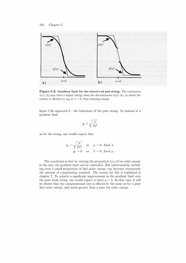
104 Chapter 5
Figure 5.2: Gradient limit for the mixed rod and string. The continuous
u(x) (a) may have a higher energy than the discontinuous u(x) (b), in which the
surface is allowed to sag at x = 0, thus reducing energy.
figure 5.2b approach 0 - the behaviour of the pure string. So instead of agradient limit
gl =√
α
2λ3
as for the string, one would expect that
gl →√
α
2λ3as µ→ 0, fixed λ
gl → 0 as λ→ 0, fixed µ.
The conclusion is that by varying the proportion λ/µ of 1st order energyin the mix, the gradient limit can be controlled. But unfortunately, includ-ing even a small proportion of 2nd order energy can increase enormouslythe amount of computation required. The reason for this is explained inchapter 7. To achieve a significant improvement in the gradient limit overthe pure weak string, one would expect to have µ ∼ λ. In that case, it willbe shown that the computational cost is effectively the same as for a pure2nd order energy, and much greater than a pure 1st order energy.

Properties of the Weak Rod and Plate 105
5.4 Hysteresis
The purpose of this section is to demonstrate that the weak plate incor-porates hysteresis for step discontinuities, just as the weak membrane did.Recall that this property imparts a tendency for edges to be unbroken, be-cause any small break causes an increase in energy. In fact, for the plate,the proof is somewhat easier than for the membrane because numerical in-tegration is unnecessary. Hysteresis for crease discontinuities has yet to beinvestigated.
Consider 2D data
d(x, y) ={
h2 if y ≥ 0−h
2 otherwisex, y ∈ [−L,L].
A weak plate represented by u(x, y) is to be fitted to d(x, y), using param-eters µ, h0, such that µ � L. Consider the case in which h > h0 so thatthe globally minimal energy state of the weak plate is u = d, with energy2αL. (There is zero energy from the plate itself, so the only contributionis the penalty generated by the step edge in u, along y = 0, of length 2L.)Now consider chopping out a small portion x ∈ [−ε/2, ε/2] from the edge,just as was done with the membrane. We seek to show that, however smallε is, there is an increase in total energy ∆E(ε), which is bounded belowby some bound greater than zero. It is sensible here to consider the limitε → 0. This would have been useless for the membrane, because pinchingthe two sections of membrane together at a point generates an ill-definedproblem.
For the plate, as ε→ 0 the decrease in penalty αε→ 0. But the plate uis forced to be continuous at (x, y) = (0, 0), no matter how small ε is. Theresulting u is “pinched together” at (x, y) = (0, 0), as in figure 5.3. Thiscauses an increase in the energy of the plate itself (not including penalties)of ∆E(0). The total change in energy for an edge gap of length ε, includingpenalties, is ∆E(ε)−αε. It is clear that ∆E(ε) is an increasing function ofε, because the continuity constraint on the plate becomes more and moreextensive as the interval [−ε/2, ε/2] lengthens. Consequently
∆E(ε)− αε > ∆E(0)− αε.
In the absence of any constraint on the plate, its energy E = 0, so theincrement ∆E(0) is the minimum, subject to the constraint u(0, 0) = 0, of
E = 2∫ L
y=0
∫ L
x=−L
{(u− d)2 + µ4(u2
xx + 2u2xy + u2
yy)}dx dy.

106 Chapter 5
Figure 5.3: Hysteresis - step discontinuities in the weak plate prefer
to be unbroken. In the global minimum energy state, the plate u fits data d
exactly (a). This is compared with the energy when u is forced to be continuous
- pinched together - at a point (b).
Since L� µ this can be taken to be approximately
E = 2∫ ∞
y=0
∫ ∞
x=−∞
{(u− d)2 + µ4(u2
xx + 2u2xy + u2
yy)}dx dy. (5.15)
By substituting X = x/µ, Y = y/µ,w = u/h, it is easily shown that
∆E(0) = Kh2µ2,
where K is a dimensionless constant.Hence the total increase in energy due to the gap
∆E(ε)− αε > Kh2µ2 − αε,
a net increase if Kh2µ2 > αε. So (using (5.7)), there is in-built resistanceto forming small gaps of length
ε < εmax = 2√
2K(h
h0
)2
µ.
The minimum gap length is of order µ. The interpretation of this result isthat, even in the presence of moderate noise, there will be a tendency toavoid gaps shorter than this minimum.
5.5 1st order plate
Because the plate has a 2nd order energy, it is expensive to compute (seechapter 7). Computation even of the continuous plate is made feasible only

Properties of the Weak Rod and Plate 107
by the use of multilevel techniques (Terzopoulos 1983), and the indicationsare that multilevel computation could confer only a limited advantage whenweak continuity constraints are in force (chapter 7). However, the weakplate problem can be reformulated as a sequence of two 1st order processes.The first is a weak membrane, applied to data d to produce a piecewisecontinuous reconstruction u in the usual way. Then a weak plate can befitted to gradient data ∇u. (Gradient ∇u is well defined, because of theregularising effect of the membrane). The fitting is constrained not to crossstep discontinuities already labelled. It is a 1st order process, minimising(in the case of quadratic variation)
E =∫ {
(p− p0)2 + (q − q0)2 + µ2(p2x + p2
y + q2x + q2y) dx dy}
+ P (5.16)
where (p0, q0) = ∇u. Results are shown in figure 5.4. Computational costis that of two 1st order processes, which is very much less than that of one2nd order process. There are of course two scale parameters in this scheme- λ1 for the membrane fitting and λ2 for the fitting of the plate to gradientdata. Practical experience suggests that it is best to choose λ2 somewhatgreater than λ1 so that the plate fitting is relatively immune to distortioncreated by the smoothing effect of the membrane.
The 1st order plate delivers step and crease discontinuities, as the trueplate does. But it does not produce a fully filtered, smooth reconstruction.Instead, it generates a piecewise continuous reconstruction u, and piecewisecontinuous surface orientation (p, q).
In practice, for reasons that the authors do not understand very clearly,use of the square Laplacian produces unstable results (figure 5.5). Thisoccurs regardless of whether the true plate or the 1st order plate is used.It may be similar to the puckering effect that Grimson (1981) observed atplate boundaries. It is uncertain whether its origin is a property of theenergy itself, or simply of the discrete approximation.
5.6 Viewpoint invariance
In the previous chapter, it was argued that a scheme for reconstruct-ing 3D surfaces should use a viewpoint invariant surface energy. For themembrane, this meant replacing the approximation 1
2 (∇u)2 dx dy by dS =(1 + (∇u)2)1/2 dx dy, the area of a surface element. Then
∫dS is invariant
because it is defined with respect to the visible surface, rather than the x, ycoordinate frame.
Quadratic variation and square Laplacian are not viewpoint invariant.They are merely approximations to certain measures of intrinsic surface

108 Chapter 5
Figure 5.4: A synthetic image (a) with added noise (b) is fitted by a weak
(quadratic variation) plate (c). Steps (black) and creases (white) are marked.

Properties of the Weak Rod and Plate 109
Figure 5.5: Instability results when square Laplacian is used in the plate (cf.
figure 5.4).
properties.The invariant equivalent of the square Laplacian (5.5) is
E =∫ {
(u− d)2 cos2 φ+ µ4(κ1 + κ2)2}dS + P (5.17)
where κ1, κ2 are principal curvatures, dS is a surface element as before andφ is surface slant. The squared sum of curvatures is expressed in the viewersframe as
(κ1 + κ2)2 =(Auxx − 2Buxy + Cuyy)2
D3, (5.18)
whereA = 1 + u2
y, B = uxuy, C = 1 + u2x and D = sec2 φ,
(do Carmo 1976). Note that A,B,C,D are all functions of 1st derivativesof u only. If the sum of squared curvatures is to be used (the invariant formof quadratic variation) then
κ21 + κ2
2 = (κ1 + κ2)2 − 2κ1κ2, (5.19)
where (do Carmo 1976) the Gaussian curvature
κ1κ2 =uxxuyy − u2
xy
D2.
As in the previous chapter, the cos2 φ term in (5.17), renders the (u−d)2term of (5.5) invariant. This correction is omitted if noise is thought to

110 Chapter 5
originate in the sensor frame rather than on the surface, to give
E =∫
(u− d)2 dx dy +∫µ4(κ1 + κ2)2 dS + P. (5.20)
Expressing the energy E as
E =∫E(ux, uy, uxx, uxy, uyy) dx dy + P,
it can be shown (Blake 1984) that the integrand E is a non-convex functionof ux, ... . So even with a fixed set of discontinuities, it is not known whetherthere is a uniquely optimal u to be found (Troutman 1983).
This problem is dealt with, in an approximate way1, by using a 1st orderplate, as already proposed for the non-invariant case. First, estimates forux(x, y), uy(x, y) are obtained by fitting an invariant weak membrane. Thislabels step discontinuities and yields estimates of ux, uy which can be in-serted as constants into E which is then convex with respect to uxx, uxy, uyy.Then E is minimised with respect to px, py, qx, qy, The integrability con-straint py = qx is not imposed, as to do so costs a great deal of computation(chapter 7).
That concludes the topic of the last two chapters - the variational anal-ysis of function fitting under weak continuity constraints. The next twochapters consider how the variational problems can be turned into discretecomputations, and how appropriate algorithms can be constructed. Themeasure of success of the algorithms will be how far the results that theyproduce agree with the theoretical predictions of the last two chapters.
1The solution is still not truly invariant, but at least the severe variations at near-extremal boundaries are greatly reduced.

Chapter 6
The Discrete Problem
The previous two chapters concentrated on exact, variational solutions toproblems with weak continuity constraints. That enabled performance tobe predicted in terms of contrast threshold, scale parameter and so on.But in order to perform function fitting with arbitrary, discrete data, theenergy E must of course be converted to a discrete form. Finite elements,first used for visual reconstruction problems by Terzopoulos (1983), are theappropriate formalism for this. They have the advantage that the accuracyof a discrete solution, as an approximation to a continuous one, is known(Zinkiewicz and Morgan 1983). Details are given, in this chapter, of discreteenergies for string, membrane and plate.
The discrete form of E is a function both of real-valued variables ui andof the boolean line-variables li that signal positions at which the continuityconstraint is broken, as explained in chapter 3. The energy E(ui, li) isto be minimised with respect to ui, li. But it was also mentioned thatminimisation with respect to li can be done “in advance”. Explicit referenceto the line process is eliminated to yield a simplified cost function F (ui),depending only on real-valued variables ui. The function F , we saw inchapter 3, is difficult to minimise, owing to its lack of convexity. A generaldiscussion of algorithms for minimising non-convex functions is given in thischapter. Then in the following chapter, our GNC minimisation algorithmis described in some detail.

112 Chapter 6
6.1 Discretisation and elimination of linevariables
To solve a functional minimisation problem computationally, it must first bediscretised. For the 1D elastic string of section 2, the simplest conceivablefinite element was used to do this - a linear element (figure 3.2 on page42). That produced a discrete expression for the energy E, as a functionof nodal values ui, and of the line variables li. Later, other finite elementswill be given for the membrane and plate in 2D. But first we describe theprocedure for elimination of line-variables from the energy for the weakstring.
To eliminate the line-process {li}, E must first be expressed as:
E = D +N∑
i=1
hα,λ(ui − ui−1, li) (6.1)
wherehα,λ(t, l) = λ2(t)2(1− l) + αl. (6.2)
and
D =N∑0
(ui − di)2 (6.3)
as before. All dependence of E on the line-process {li} is now containedin the N copies of hα,λ that appear in the formula (6.1). The functionhα,λ (plotted in fig 6.1a) governs local interactions between the {ui}. Theproblem is now (from (6.1)):
min{ui,li}
D +N∑1
hα,λ(ui − ui−1, li),
or
min{ui}
(D + min
{li}
N∑1
hα,λ(ui − ui−1, li)
)- since D does not involve the {li}. Now, immediately performing theminimisation over {li}, the remaining problem is to minimise F with respectto ui, where
F = D +N∑1
gα,λ(ui − ui−1), (6.4)
and gα,λ(t) = minl∈{0,1}
hα,λ(t, l).

The Discrete Problem 113
Figure 6.1: a) The energy function for local interaction between adjacent nodes.
b) The line process l can be eliminated from a) by minimisation over l ∈ {0, 1}

114 Chapter 6
(Often the function gα,λ will be written simply g, when this is unambiguous,and similarly for g∗, g(p) as defined in the next chapter.) The function gα,λ
is shown in fig 6.1b and is simply the minimum of the 2 graphs in fig 6.1a.Explicitly, gα,λ is
gα,λ(t) ={λ2t2 if |t| <
√α/λ
α otherwise. (6.5)
The line process l can be explicitly recovered, at any time, from g(t) by asimple formula:
l ={
1, if |t| >√α/λ
0 otherwise. (6.6)
6.1.1 Extending 1D methods to 2D
The natural extension to 2D of the linear element used above, is a lineartriangular element. Within each element, u(x, y) is linear and determinedby 3 nodal values as in fig 6.2. Line-variables on each triangle, as shown,
Figure 6.2: Linear triangular elements for the membrane. Line-variables
li,j , mi,j are attached to each triangle. However, this arrangement of line-variables
may prove inconvenient in practice (see text).
indicate (li,j = 1 or mi,j = 1) when a discontinuity exists, disabling theenergy of that triangle, and incurring a penalty α. Along a contour ofdiscontinuity, a whole chain of triangles is disabled, each accruing a penaltyα. The total penalty P , incorporated in energy E, is therefore equal to α

The Discrete Problem 115
times the total length of all discontinuity contours, and that is just asrequired (chapter 4). The resulting energy, analogous to (6.1) above, is
E = D +∑i,j
hα,λ
(√(ui,j − ui−1,j)2 + (ui,j − ui,j+1)2, li,j
)(6.7)
+∑i,j
hα,λ
(√(ui,j − ui+1,j)2 + (ui,j − ui,j−1)2,mi,j
)where now
D =∑i,j
(ui,j − di,j)2. (6.8)
Line variables can be eliminated, replacing h with g as before, to obtain anenergy F (u). As in chapter 3, it is necessary to construct a convex approx-imation F ∗. This proves to be particularly difficult for the arrangement ofelements and line-variables in figure 6.2. It turns out that it is no longerfeasible to guarantee, as we can for the string (see next chapter), that F ∗
is as close as possible to F whilst still being convex. Additional inefficiencyarises because of the need to compute the square roots in (6.7).
Instead, a different arrangement of line-variables is adopted, whosephysical role is perhaps a little less sympathetic to the spirit of finite ele-ments, but which facilitates construction of a convex approximation. Thenew discrete energy is
E = D +∑i,j
hα,λ (ui,j − ui−1,j , li,j) +∑i,j
hα,λ (ui,j − ui,j+1,mi,j) . (6.9)
Now li,j = 1 flags the collapse of two adjacent triangles in a Northerlydirection, as in fig 6.3. And mi,j = 1 flags the collapse of a pair of triangles,but in an Easterly direction. Line-variables in (6.9) can be eliminated togive the 2D equivalent of (6.4):
F = D +∑i,j
g(ui,j − ui−1,j) +∑i,j
g(ui,j − ui,j+1). (6.10)
Line-variables are recovered as before, from (6.6).The viewpoint invariant membrane, described earlier in chapter 4, must
use the original triangulation scheme (figure 6.2). This is because the gra-dient term in the energy integrand is
√1 + u2
x + u2y so that the two compo-
nents u2x, u2
y are not separable. But, as before, the convex approximationis less satisfactory.
From the point of view of 2D rotational invariance, equilateral triangularelements would actually be preferable. Of course they may be inconvenient

116 Chapter 6
Figure 6.3: When line-variable li,j = 1, this signifies that the “Northerly”
component of the energy of the membrane, over the 2 triangles shown, is disabled.
Similarly for mi,j = 1, but acting in an Easterly direction.

The Discrete Problem 117
for use with the usual rectangularly formatted images, but are in keepingwith the hexagonal tesselation of retinal mosaics. They are better becausethey enable more precise measurement of contour lengths (in the term P ),as shown in figure 6.4. Imagine Manhattan built with hexagonal blocks -distances by road would be reduced, and would be much closer to distanceas the crow flies. Hexagonal tesselation would make sensitivity to contrast,in the weak membrane, vary far less with varying orientation of contours.In fact variations are reduced by a factor of almost 3, from about ± 18%to about ± 7%. In practice, however, an approximately square grid is used.
Figure 6.4: Rotational invariance of length measurement is greatly improved
on a hexagonal grid.
As expected, sensitivity is greatest for horizontal and vertical lines, andleast for diagonal ones. (See, for example, some of the images in figure 4.1on page 53.
6.1.2 Higher order energies: weak rod and plate
Since energies for the rod (1D) and the plate (2D) include 2nd derivativesof the fitted function u, linear elements are inadequate (having zero 2ndderivative). The 1D case is an obvious specialisation of the 2D one, sothe following discussion is restricted to the plate. The simplest element,though somewhat unorthodox, is the non-conforming quadratic element ofTerzopoulos (1983), developed for the smooth, thin plate. It is unorthodoxin having nodes which lie outside the element itself - see fig 6.5. Valuesof 2nd derivatives within the (i, j)th element are simple functions of nodal

118 Chapter 6
Figure 6.5: The non-conforming, square, quadratic element of Terzopoulos has
6 nodes, 2 of which lie outside the square. For the weak plate, a line-variable li,jis associated with each element.

The Discrete Problem 119
values:
uxx = ui,j−1 + ui,j+1 − 2ui,j , (6.11)uyy = ui−1,j + ui+1,j − 2ui,j ,
uxy = −ui,j − ui+1,j+1 + ui,j+1 + ui−1,j .
As mentioned in chapter 5, there is in fact a one parameter familyof suitable (rotationally invariant) 2nd order energy functions (Grimson1981, Brady and Horn 1983). They are the linear combinations of thesquare Laplacian (5.5) and the quadratic variation (5.4). Quadratic vari-ation proves more awkward to handle, because line-variable eliminationgenerates the following energy:
F = D +∑i,j
gβ,µ2
(√Vi,j
)(6.12)
where Vi,j is the discrete form of quadratic variation
u2xx + 2u2
xy + u2yy,
in which uxx, uxy, uyy are each represented discretely as in (6.11). This isinefficient for much the same reasons that the ideal membrane scheme withtriangular elements (see above) is inefficient: the convex approximation F ∗
is not as good, and square roots must be computed. The square Laplacianenergy gives a simpler computational scheme, with just one line-variableper element. After elimination of line-variables, the energy of the weakplate is
F = D +∑i,j
gβ,µ2(ui,j−1 + ui,j+1 + ui−1,j + ui+1,j − 4ui,j) (6.13)
similar to (6.4) for the membrane, but with parameters µ2, β in place ofλ, α, and the argument of gβ,µ2 being a discrete Laplacian of u rather thana first derivative. In practice, the Laplacian scheme exhibits instability onboundaries (figure 5.5, page 109).
As before (6.6), after F has been minimised, line-variables li,j can berecovered. But now the interpretation of line-variables is a little differentthan for the membrane. In 1D (the rod), for example, a single line-variablewith the value li = 1 indicates a gradient discontinuity (a crease). Twoadjacent line-variables with values li = 1, li+1 = 1 indicate a step. In 2D,a crease appears as a contour along which the line-variables are set. A stepappears as a thick contour of set line-variables, two elements wide. And awide step (as occurs in intensity data, at shadow boundaries) is labelled asa tramline - a pair of parallel contours.

120 Chapter 6
6.1.3 First order plate
Since the computational cost of schemes employing 2nd order energies willprove to be high a more economical way of achieving a similar effect isneeded. In the previous chapter, it was shown that the weak plate com-putation can be split into two 1st order computations. The first is theordinary membrane, already discussed, which produces step discontinuitiesand a surface u(x, y). The surface can be differentiated to give
p0(x, y) = (p0(x, y), q0(x, y)) = ∇u(x, y)
whose discrete form
p0i,j = (ui,j − ui,j+1, ui,j − ui−1,j)
can be used as data for a second 1st order process to reconstruct gradi-ent pi,j , complete with discontinuities. These represent 1st order (crease)discontinuities in the original data di,j .
The gradient reconstruction operates by minimising
F =∑i,j
{‖pi,j − p0
i,j‖2 + g(√
Vi,j
)}(6.14)
where Vi,j is quadratic variation, as before, but now expressed in terms ofpi,j :
Vi,j = (pi,j − pi−1,j)2 + (pi,j − pi,j−1)2 + (qi,j − qi−1,j)2 + (qi,j − qi,j−1)2
Note that there is no attempt to impose the integrability constraint thatpy = qx, although we have a perfect right to do so. The reason is thatcomputation time to minimise F would be severely increased, as shown inthe next chapter.
6.1.4 Sparse data
So far, energies have been given for the case in which data is dense. Stereo-scopic depths, remember, are not dense but are sparsely and irregularlydistributed in the image planes. A simple modification to the energy takescare of this. Suppose that data dk is available at points (ik, jk), k = 1, ..,K.The “faithfulness to data” component D of energy (6.8) must be replacedby
D =A
K
K∑k=1
(uik,jk− dk)2 (6.15)
Other energy terms are unchanged.

The Discrete Problem 121
6.2 Minimising convex energies
What makes the discrete problems difficult to solve is the fact that discon-tinuities are incorporated into the reconstructed functions. In this sectiona little time is taken out to discuss the simpler problem of reconstructingsurfaces which are entirely continuous, before proceeding to consider howto solve the main problem.
This class of problem was extensively examined by Grimson (1981) andTerzopoulos (1983). In chapter 2 it was concluded that continuous recon-struction has limited application. That was because the most compellingreason for going to the computational expense of explicit surface recon-struction is to pick out discontinuities masked by texture. A surface fittingscheme to do this must be able to recover discontinuities which are a prioriunknown, and localise them accurately.
However, there are one or possibly two ways in which continuous recon-struction of depth data can be useful. The first is in converting sparse datato dense, using a continuous membrane to do the “filling-in” (McLauchlanet al. 1987). The data is then in a more convenient form for reconstructionwith discontinuities, for reasons that were given in chapter 4. The seconduse is that, as was pointed out in chapter 2, it might be convenient to havea depth map available for path planning and collision avoidance. Again,a membrane is quite adequate; there is no reason to go to the expense ofreconstructing a smooth surface by means of a plate.
6.2.1 Algorithms based on gradient descent
Energies for continuous surfaces can be obtained by “disabling” the lineprocesses in the energies defined earlier. Since the membrane with sparsedata is the process that is of most interest, that is the one considered here.Line variables in (6.9) are switched off -
li,j = mi,j = 0
- to give the energy for the continuous membrane:
E = D +∑i,j
hα,λ (ui,j − ui−1,j , 0) +∑i,j
hα,λ (ui,j − ui,j+1, 0)
= D + λ2
∑i,j
(ui,j − uu−1,j)2 +∑i,j
(ui,j − ui,j+1)2
. (6.16)
The error term D for sparse data was defined in (6.15). If, for some reason,it is known that the surface u is discontinuous along some contour, then

122 Chapter 6
the energy is modified simply by clamping the line variables “on” (li,j =1,mi,j = 1) at all points along the contour. Similarly, if the fitting processis restricted to some irregularly shaped region, such as a region alreadyfound to contain image texture, line variables are clamped on along theregion boundary.
With all line variables fixed, minimisation of E is an entirely classicalproblem. The condition for u to be the desired minimum is that
∂E/∂ui,j = 0, ∀i (6.17)
- the gradient of E (with respect to u) vanishes. Energy E is a quadraticfunction of u, so this is a system of linear simultaneous equations. What ismore, the fact that E is “strictly convex” (see next chapter for discussionof convexity) guarantees that there is one and only one solution.
There are numerous ways to solve such an equation, most of which in-volve successive adjustments of the ui,j to reduce E, until it can be reducedno further. The crudest way to do that is simply to try small changes toeach of the ui,j in turn, and to accept changes which reduce E. (That wasthe method described, at the end of chapter 3, to find a minimum of thefunction F (p).) It does work, but can be inefficient. A better strategy isto use the gradient ∂E/∂ui,j as a guide to how ui,j should be changed,in order to reduce E fastest. Grimson (1981) used the “conjugate gradi-ent” algorithm to minimise the energy of a plate. Terzopoulos (1983) usedthe “Gauss-Seidel” algorithm, which is a special case of the “SuccessiveOver-relaxation” (SOR) algorithm.
SOR works as follows. For each site (i, j), gradient ∂E/∂ui,j is com-puted, and the the quantity
w
T(∂E/∂ui,j)
is subtracted from ui,j . The constant T is carefully chosen to ensure conver-gence whenever w ∈ (0, 2). The whole process is repeated many times (thenext chapter tells just how many) until the solution is reached. This algo-rithm (SOR) is laid out explicitly, in the case of a membrane with sparsedata, in figure 6.6. Note that the “Gauss-Seidel” algorithm is the specialcase of SOR in which w = 1. As it stands, the algorithm is serial, becausethe ui,j are updated in strict sequence. Parallel versions do, however, exist:“simultaneous over-relaxation” and “chequerboard SOR”.
6.2.2 Multi-grid algorithms
Terzopoulos greatly enhanced the basic SOR algorithm by making use ofmulti-grid techniques (Brandt 1977), in which relaxation takes place simul-taneously, on coarse and fine arrays. Use of four arrays, with density in

The Discrete Problem 123
Nodes: i ∈ {0, ..., N}, j ∈ {0, ..., N}.Iterate n = 1, 2, ...
For i = 1, ..., N − 1, j = 1, ..., N − 1:If there is data at node {i, j}:
u(n+1)i,j = u
(n)i,j − ω
{(1 + 4λ2
)u
(n)i,j − di,j − λ2
(u
(n+1)i−1,j + u
(n+1)i,j−1
+u(n)i+1,j + u
(n)i,j+1
)}/(1 + 4λ2
)otherwise:
u(n+1)i,j = u
(n)i,j − ω
{4u(n)
i,j −(u
(n+1)i−1,j + u
(n+1)i,j−1
+u(n)i+1,j + u
(n)i,j+1
)}/4
Modification is necessary at corners, for example:If there is data at node {0, 0}:
u(n+1)0,0 = u
(n)0,0 − ω
{(1 + 2λ2
)u
(n)0,0 − d0,0 − λ2
(u
(n)1,0 + u
(n)0,1
)}/(1 + 2λ2
)otherwise:
u(n+1)0,0 = u
(n)0,0 − ω
{2u(n)
0,0 −(u
(n)1,0 + u
(n)0,1
)}/2.
Modification is also necessary on array edges, for example:If there is data at node {0, j}, 1 ≤ j ≤ N − 1:
u(n+1)0,j = u
(n)0,j − ω
{(1 + 3λ2
)u
(n)0,j − d0,j − λ2
(+u(n+1)
0,j−1
+u(n)1,j + u
(n)0,j+1
)}/(1 + 3λ2
)otherwise:
u(n+1)0,j = u
(n)0,j − ω
{3u(n)
0,j −(u
(n+1)0,j−1 + u
(n)0+1,j + u
(n)0,j+1
)}/3.
Figure 6.6: An SOR algorithm for the membrane, with sparse data.

124 Chapter 6
the ratios 8:4:2:1, achieved a speed-up in excess of 100:1, for the continuousplate. In our case, speed-up for the membrane (McLauchlan et al. 1987) istypically 10:1 (somewhat dependent on the scale λ and the sparsity of thedata).
The principle of multigrid operation is illustrated in figure 6.7. The
Figure 6.7: Multigrid relaxation. In this illustration, grids are shown at
three levels. Relaxation takes place on coarse and fine grids, moving both upwards
and downwards in order to achieve fastest convergence.
problem is that standard SOR, at a single level, rapidly smooths awayerror signals of high spatial frequency, leaving a persistent low frequencyerror that decays slowly. This happens because each iteration of relaxationis a local process; high frequencies are removed locally, but low frequenciesrequire long distance propagation, taking many iterations. That is wherecoarse grids help. Low spatial frequencies, projected onto a coarse grid,become high frequencies with respect to the new grid. To put it anotherway, neighbour to neighbour communication on a coarse grid covers moreground per iteration than on a fine grid. An adaptive scheme switches therelaxation process between levels (both coarse to fine and fine to coarse).Switching occurs according to the spectral composition of the error signal,as measured by local Fourier transformation. For the membrane, “chequer-board Gauss-Seidel” was found to be most effective. Imagining the gridat each level to be a chessboard, all the black squares are updated in oneiteration, and all the white ones in the next. This means that, in any oneiteration, each square that is updated has four nearest neighbours that are

The Discrete Problem 125
left alone. There is no interaction, therefore, between any pair of squaresbeing updated. Thus the order of updating does not matter, and thereforecomputation is truly parallel within each iteration.
6.3 Overcoming non-convexity
Let us now return to the main problem - dealing with weak continuityconstraints. The energy functions F for weak continuity problems are non-convex. Convexity is a sufficient condition for all local minima to be globalminima. Since F is non-convex it may have many local minima, many ofwhich are not global. We showed in section 2 that F does in fact havemany local minima - possibly as many as 2N , for a weak elastic string withdata vector d0, .., dN . This means that naive gradient descent will almostcertainly stick at a local minimum that is of higher cost than the globalminimum. What is more, which local minimum is reached will dependstrongly on the starting point of the descent. For this reason, it was ar-gued in chapter 3 (where our myopic fly remained trapped at altitude), analgorithm is needed that has some ability to “look ahead”.
6.3.1 The GNC algorithm
This book proposes the GNC algorithm, already described briefly in chapter3, and due to be explained fully in the next chapter. The algorithm givenin chapter 3 (figure 3.7, page 49) worked by direct descent, trying smallchanges in each of the ui in turn, and accepting them if they reduce theenergy function F (p). More sophisticated gradient following methods (SOR)are described in the next chapter. For now, recall the central step of theearlier algorithm: to test a small increment (or a decrement) δ in ui andcompute the energy change
∆F (p) = F (p)(u1, .., ui + δ, .., uN )− F (p)(u1, .., ui, .., uN ). (6.18)
If ∆F (p) < 0 then the change is accepted. This operation is applied insequence to the ui, to comprise one iteration. Iterations are repeated, fora given p, until convergence. Non-convexity parameter p is decreased from1 (convex) towards 0 (true energy function).
There are three main alternatives to GNC, each somewhat different innature. All three are algorithms of general applicability, whereas GNC issomewhat special to problems involving weak continuity constraints - whichis both its weakness and its strength.
The first of the alternatives is simulated annealing. Kirpatrick et al.(1982) described its application to the minimisation of non-convex energies.

126 Chapter 6
Smith et al. (1983) used it for image restoration. Geman and Geman (1984)also applied it to image restoration, using a cost function that incorporatesweak continuity constraints.
The second is Hopfield’s neural network computation (Hopfield 1984).It involves constructing a single energy function which is a compromisebetween the true F and a convex approximation to F . This compromisefunction is somewhat like F (p) in the GNC algorithm, for some intermediatevalue of p ∈ [0, 1]. His method of obtaining the convex F ∗ is generallyapplicable to integer programming problems, but at the price of being arather poor approximation compared with the F ∗ used in GNC.
Finally dynamic programming (Bellman and Dreyfus 1962), previouslyused for curve detection by Montanari (1971), has been successfully appliedto the weak string by Papoulias (1985).
6.3.2 Simulated annealing
Simulated annealing is a powerful, general method for finding global optimaof functions which have many local optima. It is based on the algorithmof Metropolis et al. (1953) for simulating statistical mechanical systems.Instead of direct descent, some randomness is introduced into the descentpath. This avoids sticking in local minima. The degree of randomnessis controlled by a temperature parameter, which is initially high. As thesystem approaches the global minimum, it is allowed to cool.
The structure of the algorithm is superficially similar to GNC. Insteadof sweeping parameter p from 1 to 0, a temperature T is reduced from somestarting value towards 0. And in place of the deterministic updating rule,increments δ in each ui are tested according to a random rule. The energychange is defined, similarly to (6.18), but for the actual cost function F ,rather than for F (p):
∆F = F (u1, .., ui + δ, .., uN )− F (u1, .., ui, .., uN ). (6.19)
The following rule is then applied: if ∆F < 0 then the change is acceptedas before, but if ∆F ≥ 0 then it is accepted randomly, with probability
exp (−∆F/T ) ,
and otherwise rejected. The schedule for reduction of temperature is given(Geman and Geman 1984) by
T = C/ log(1 + k)
at the kth iteration, where C is an appropriate energy constant, related toa characteristic energy of the system. When T is large, energy increases

The Discrete Problem 127
are often accepted, enabling the system to jump out of local minima. AsT → 0, the system “freezes”, becoming almost deterministic in its descenttowards a minimum of energy.
The generality of simulated annealing is a great attraction. Simulatedannealing can, in a sense, be regarded as a general engine for non-convexproblems. It can be argued however that the additional freedom to choosea cost function for simulated annealing is not of great benefit for visualreconstruction problems. For example, a more complex line process (Gemanand Geman 1984) can be used to penalise breaks and endings of edges. Butthe hysteresis effect, intrinsic to the membrane and plate, already do thatvery satisfactorily. In any case, computational requirements can escalatealarmingly if an “arbitrary” energy is designed at will. This is illustratedin the next chapter, where it is shown that energies of second or greaterorder necessarily demand much more computation than first order ones.
Comparison of efficiency is difficult, since execution times are stronglydependent on data and on precise choice of energy function. Executiontime of GNC, for instance, increases markedly when the data is very noisy(see later), and this may also be the case with simulated annealing. Typicalreported runtimes for simulated annealing with energies most closely com-parable to ours are around 1000 iterations (Marroquin 1984). Equivalentruntime for GNC can be as low as 50 iterations, tending to be higher atlarge spatial scale λ, µ. Another significant advantage of GNC over simu-lated annealing is the potential for implementation in conventional analoguehardware, without the need to use noise generators.
6.3.3 Hopfield’s neural model
Hopfield’s neural model (Hopfield 1984) solves certain boolean program-ming problems. It can be expressed1 as the minimisation of an energyF (0), where
F (p) = −12
∑i,j
Ti,jViVj +∑
i
IiVi +∑
i
Z(p)i (Vi), (6.20)
with respect to Vi ∈ [0, 1]. Constants Ti,j and Ii between them encode prob-lem constraints and data. The function Z(p), plotted in figure 6.8, controlsconvexity, just as in GNC. The final configuration of the Vi represents thesolution. Variables Vi are allowed to take real values in the range [0,1], butas p→ 0 they are forced naturally towards boolean values2 0,1.
1The notation here is slightly altered from Hopfield’s original, so as to make theanalogy with GNC clear.
2In Hopfield’s formulation, the Vi take values −1, 1, but that is a minor detail.

128 Chapter 6
Figure 6.8: Control of convexity in Hopfield’s system. When p = 0, the
rectangular energy function forces solutions to be boolean-valued.
It is desired to minimise the energy for p = 0; unfortunately F (0) is non-convex. In the limit p→ 1, F (p) becomes convex, but of course with totallydifferent extrema. Hopfield’s procedure uses F (p) with an intermediatevalue of p. Recent work suggests that, as in GNC, sweeping p from 1 to0 may be useful in the neural model (Hopfield and Tank 1985). Whereassuch a strategy will be proven, in the next chapter, to be effective in GNC,there are as yet no corresponding proofs for neural networks.
The main difference from GNC is that the convex approximation F (1)
in (6.20) is by no means a close one, though general for a certain class ofinteger problems. If only one value of parameter p is used, rather thansweeping p, the solution is not necessarily an extremum of the originalfunction F . Moreover, optimisation of a convex F (p) in Hopfield’s methodneed not yield the solution for F (0), because the extrema of such F (p) arenot generally integer solutions Vi ∈ {0, 1}. In GNC, however, F (1) is oftena sufficiently good approximation to F (0) to yield a correct solution.
In any case, an exact comparison of the methods is difficult becausethey solve different problems. The Hopfield scheme might be made toimplement a weak string, for example, by extending it to deal with mixedreal and boolean variables (Yuille 1985). The energy (6.20) would becomea cubic polynomial in ui, li (taking the place of the Vi above), as in (3.3)on page 42.
6.3.4 Dynamic programming
Dynamic programming is a technique for optimising functions of discretevariables, applicable when the function F can be decomposed as a sum of

The Discrete Problem 129
many functions, each with just a few arguments. Since dynamic program-ming requires discrete valued variables, the variables ui must be quantisedinto M discrete levels.
A dynamic programming algorithm to minimise the energy F of theweak string runs as follows. First “return functions” φk are defined andcomputed by a recurrence relation:
φ0(u1) = minu0
{(u0 − d0)2 + g(u1 − u0)
}φk(uk+1) = min
uk
{(uk − dk)2 + g(uk+1 − uk) + φk−1(uk)
}, 1 ≤ 1 < N.
The minimisation here must be done by brute force, testing for each possiblevalue of uk in succession. As they are computed, the minimising value uk, inthe definition of φk above, defines the value of “policy functions” ψk(uk+1).Each policy function is stored as an M -element table. Now, as a startingcondition, set uN to the value that minimises
(uN − dN )2 + φN−1(uN ).
The bulk of the work has been done; all that remains, in order to determinethe optimal ui, is a single reverse scan. For k = N−1, ..., 0 perform a singletable lookup to compute
uk = ψk(uk+1).
The method has the great advantage of being exact, regardless of con-vexity. This is because it is essentially an ordered search over all possiblevalues of all variables. Unlike direct descent, it makes no use of the localsmoothness of the function F . Papoulias (1985) implemented a dynamicprogramming algorithm for the weak string. He showed that, for data el-ements of length N , the time complexity of the algorithm is O(NM2).Storage requirement is O(NM).
Papoulias pointed out that the use of dynamic programming is im-practical for the weak rod, for which the functions f above have not twobut three variables. Time complexity rises to O(NM3) and storage toO(NM2). Since typical values are N = M = 100, runtime on a microcom-puter increases from about 1 minute to about 1 hour. For 2D problems, themembrane and the plate, dynamic programming is quite unusable. This isbecause, although the energy function F partitions much as in 1D, there isno natural ordering of the variables in a 2D array.

130 Chapter 6

Chapter 7
The GraduatedNon-Convexity Algorithm
At the end of the last chapter, the various methods available for solvingnon-convex problems were reviewed. Now, the method proposed in thisbook - the GNC algorithm - will be described in some detail. In chapter 3we saw that there are two main steps. The first is to construct a convexapproximation to the non-convex function, and then proceed to find itsminimum. The way in which such a function can be constructed will beexplained - for the weak string, and then for a more general case. Thesecond step is to define a sequence of functions, ending with the true costfunction, and to descend on each in turn. Descent on each of these functionsstarts from the position reached by descent on the previous one.
Such a procedure is certainly intuitively appealing. It is unlikely thatvery strong general statements can be made about its effectiveness for anarbitrary non-convex cost function. But, in the case of the energy functionsthat describe the weak string and membrane, the algorithm can be shownto be correct (section 7.3) for a significant class of signals. Performance ofthe computer implementation also reflects faithfully the variational truthsof chapter 4. It will become apparent that this is a consequence of theparticular convex approximation F ∗ that has been defined. Other plausibleconvex approximations, when used in a GNC procedure, fail to find globalminima.
Convergence properties of the algorithm are derived. It is this that leadsto the conclusion that 2nd order schemes must require far more computationthan 1st order ones. Moreover, imposing an integrability constraint in thesecond stage of the 1st order plate - natural though it would be to do
132 Chapter 7
so - would result in very slow convergence. Optimal values for relaxationparameters are computed. Relaxation algorithms are summarised in a waythat would, hopefully, enable the reader to implement them.
7.1 Convex approximation
7.1.1 Weak string
Recall that the energy
F = D +N∑
i=1
g(ui − ui−1)
is to be approximated by a convex function
F ∗ = D +N∑
i=1
g∗(ui − ui−1)
by constructing an appropriate neighbour interaction function g∗. This isdone by “balancing” the positive second derivatives in the first term D =∑
i (ui− di)2 against the negative second derivatives in the g∗ terms. Thebalancing procedure is to test the Hessian matrix H (Roberts and Varberg1976) of F ∗: if H is positive definite then F ∗(u) is a convex function1 of u.
The Hessian H of F ∗ is
Hij =∂2F ∗
∂ui∂uj= 2Ii,j +
∑k
g∗′′(uk − uk−1)Qk,iQk,j , (7.1)
where I is the identity matrix and Q is defined as follows:
Qk,i = ∂(uk − uk−1)/∂ui =
1 if i = k−1 if i = k − 10 otherwise.
Now suppose g∗ were designed to satisfy
∀t g∗′′(t) ≥ −c∗ (7.2)
where c∗ > 0. Then the “worst case” of H occurs when
∀k g∗′′(uk − uk−1) = − c∗,
1In appendix D.2 it is shown that positive definite H means F ∗ is convex, even whenthe 2nd derivative of g∗, and hence the 2nd partial derivatives of F ∗, are discontinuous,as they are for the g∗ defined below in (7.7).

The Graduated Non-Convexity Algorithm 133
so thatHi,j = 2Ii,j +
∑k
(−c∗)Qk,iQk,j (7.3)
orH = 2I − c∗QTQ. (7.4)
To prove that H is positive definite, it is necessary simply to show that thelargest eigenvalue vmax of QTQ satisfies
vmax ≤ 2/c∗. (7.5)
In appendix D.1 it is shown that this really is a worst case: convexity of Hin (7.3) does guarantee convexity of H in the general case (7.1).
Construction of a function g∗ with a given bound −c∗ as in (7.2) isrelatively simple. Suppose the extra condition is imposed that
∀t g∗(t) ≤ g(t), (7.6)
then the best such g∗ (closest, pointwise, to g) is obtained by fitting aquadratic arc of the form − 1
2c∗t2 + bt+ a to the function g(t), as shown in
fig 7.1. The definition of g∗ ≡ g∗α,λ is now:
Figure 7.1: The local interaction energy function g of fig 6.1 is modified to func-
tion g∗, in order to produce a cost function F ∗ that is convex, and approximates
F .
g∗α,λ(t) =
λ2(t)2, if |t| < qα− c∗(|t| − r)2/2, if q ≤ |t| < rα, if |t| ≥ r
(7.7)
where
r2 = α
(2c∗
+1λ2
), and q =
α
λ2r. (7.8)

134 Chapter 7
All that remains now is to choose a value c∗ by determining the largesteigenvalue vmax of QTQ. Then, to satisfy (7.5) while keeping c∗ as smallas possible (so that g∗ is as close as possible to g), we choose
c∗ = 2/vmax. (7.9)
For example, for the string, it is shown in appendix D that the largesteigenvalue vmax = 4, so from (7.9) c∗ = 1
2 .
7.1.2 General method
In general, for all 1D and 2D problems, our function F has the form:
F (u) = D +∑
k
gk(u) (7.10)
where gk(u) = g
(∑l
Qk,lul
)(7.11)
with g as before2 and Q is a “circulant” matrix, representing a convolutionoperation defined by an array C. For example, for the 1D weak string, thecirculant matrix Q would be
Q =
. . . . . . . . . . . . . . . . . .. . . −1 1 0 0 . . .. . . 0 −1 1 0 . . .. . . 0 0 −1 1 . . .. . . . . . . . . . . . . . . . . .
(7.12)
and the corresponding convolution is
C =(. . . 0 −1 1 0 0 . . .
),
which means
Ck =
−1 for k = −11 for k = 00 otherwise.
It can be seen that matrix Q is simply made up of rows which are succes-sively displaced copies of C. That is the definition of a circulant Q. For2D problems like the membrane, index k in (7.10) is a double index. Theconvolution C is therefore a two dimensional array, so the circulant Q is
2Note that the functions g, g∗, as defined above, do not quite apply to quadraticvariation, or to the invariant membrane. They can be suitably modified however.

The Graduated Non-Convexity Algorithm 135
four-dimensional! Strictly, Q is a circulant only if the computational arrayis considered to be circular (or toroidal in 2D). To account for boundaryconditions on array borders, Q is slightly modified. But this doesn’t reallyaffect the computation of eigenvalues, as is shown in appendix D.4.
Now, replacing g by g∗ in (7.10), to obtain
F ∗(u) = D +∑
k
g∗k(u) (7.13)
where g∗k(u) = g∗
(∑l
Qk,lul
)its Hessian can be computed.
Hij =∂2F ∗
∂ui∂uj= 2 +
∑k
g∗′′(∑
l
Qk,lul
)Qk,iQk,j . (7.14)
In the worst caseH = 2I − c∗QTQ,
which is positive definite if the largest eigenvalue of QTQ satisfies
vmax ≤ 2/c∗.
So g∗ is as defined in (7.7) with
c∗ = 2/vmax.
The calculation of vmax, for the weak string, rod, membrane and plateappears in appendix D.3. The task is made relatively easy by the fact thatQ is (almost) a circulant, so that there is a formula (Davies 1979) whichgives all its eigenvalues. The results are summarised in the following table.
c∗
string 1/2
membrane 1/4
rod 1/8
plate (Laplacian) 1/32
The value given for the plate is for the square Laplacian, since an exactvalue cannot readily be obtained for quadratic variation. Similarly, exact

136 Chapter 7
values cannot conveniently be computed for the invariant membrane. It isalmost as useful to have a lower bound on c∗ since that can also be usedto construct a convex function, though not necessarily the closest one. Inthe GNC algorithm, to be described next, this simply has the effect ofwasting some computation on “more than convex” approximations, beforethe “closest” convex approximation is reached.
7.1.3 Convex approximation for sparse data
The foregoing discussion of convexity does not apply to reconstruction di-rectly from sparse data. This is because the component D that describesadherence to data, as we saw in the previous chapter, is
D =A
K
K∑k=1
(uik,jk− dk)2
rather thanD =
∑i,j
(ui,j − di,j)2.
Since it is not known a priori at which points (ik, jk) there is a data elementdk, no component of D can be “relied upon” to be present. It is necessaryto be able to construct an approximation F ∗ that is convex even when (dataof unlimited sparsity!) the D term is altogether absent. From (7.13), if theD term is absent,
F ∗(u) =∑
k
g∗k(u) (7.15)
with g∗k(u) = g∗
(∑l
Qk,lul
), (7.16)
so it is clear that g∗(t) itself must now be convex. This can be done fort lying in some finite range, as shown in figure 7.2. But the resultingg∗ is not nearly such a close approximation to g as for the dense case.Anyway, because of the ambiguity problem discussed in chapter 4, directreconstruction from sparse data is not recommended. Instead, sparse datais first converted to dense using a continuous membrane, using small spatialscale λ to avoid distortion.
This discussion of sparse data also underlines a general principle. Themore carefully the specific structure of energy F is taken into account, thecloser the convex approximation F ∗ can be made. In the case of sparsedata, a rather general approach had to be used for construction of F ∗, sothe approximation cannot be as good as it was for dense data. Even so,

The Graduated Non-Convexity Algorithm 137
Figure 7.2: With sparse data, a convex cost function F ∗ is constructed by
replacing g by g∗, over some finite interval. But the approximation is much
poorer than for dense data (fig 7.1).
specific structure was taken into account insofar as line variable eliminationwas still incorporated, so that the energy has the form F (u). Withoutthat, the energy would have had the form E(u, l), for which it is difficultto obtain a convex approximation at all, even by the most general methods(for example Hopfield’s method as in the previous chapter).
7.2 Performance of the convexapproximation
Minimisation of the convex approximation F ∗ is only the first of two stepsof the GNC algorithm. But before proceeding to define the second step, itis worth looking at the performance of the first step, in its own right. Afterall, having constructed an approximation to the cost function F , mightit not be sufficient to minimise that? The answer is “sometimes” - if thespatial scale constant λ is small enough. But for larger λ, we shall see thatit is essential to proceed to the second step of GNC.
When is the global minimum of F ∗, which can be found by gradientdescent, also the global minimum of F? A completely general answer, thatapplies for any data d, cannot be given. But certain strong results can beobtained for a class of data comprising “isolated” steps and including noise.
The conclusion of the analysis turns out to be that F ∗ behaves exactlylike F except when the step height h is close to the contrast sensitivitythreshold h0. Just how close depends on λ. If λ ≈ 1 then h must bequite close to h0 before F ∗ starts to behave badly. But if λ � 1 then F ∗
behaves badly almost all the time. Intuitively, the result that F ∗ works well

138 Chapter 7
only for small λ is plausible when one considers g∗α,λ which approximatesgα,λ well only for small λ, as figure 7.3 shows. Hence F ∗ is a much closer
Figure 7.3: Neighbour interaction function g∗α,λ is a much better approximation
to gα,λ for λ ≈ 1 (a) than for λ � 1 (b).
approximation to F when λ is small. These observations apply also to themembrane, and (substituting µ2 for λ) to the rod and plate.
A test for success in optimising F ∗ (in the sense that the minimum u∗
of F ∗ is also the global minimum of F ) is that:
F ∗(u∗) = F (u∗). (7.17)
Graphical justification of this was given in figure 3.6 on page 48. Thealgebraic justification is also simple: g∗ is defined (7.6,7.7) in such a waythat
∀t, g∗(t) ≤ g(t)
(with equality for |t| ≤ q and |t| ≥ r). This means, from (7.10) and (7.13),

The Graduated Non-Convexity Algorithm 139
that∀u, F ∗(u) ≤ F (u)
Combining this with the definition of u∗, that
∀u, F ∗(u∗) ≤ F ∗(u),
and with (7.17) gives∀u, F (u∗) ≤ F (u). (7.18)
So when (7.17) holds u∗ is the global minimum of F .Once u∗ has been computed, a formula like (6.6) on page 114 that is
used with F , is needed to recover the line variables. It is obtained from thedefinition (7.7) of g∗:
li =
1, if |ui − ui−1| > r0, if |ui − ui−1| < qambiguous otherwise.
(7.19)
It is easily seen that if and only if no line variables come up ambiguousthen condition (7.17) is satisfied, and the convex optimisation has beensuccessful. Otherwise the ambiguity must be resolved by the second stepof the GNC algorithm. An example of how this works in practice is givenin figure 7.4.
In appendix E the minimisation of F ∗ for the weak string applied to anideal step of height h, is solved. A recurrence relation is obtained for thecomponents u∗i of u∗. It is shown that if the effective height h of the stepis large enough, or small enough, the test (7.17) succeeds. For intermediatestep heights, however, it fails because at least one of the line variables isambiguous in (7.19). The range [h−, h+] of intermediate step heights, whichincreases as λ increases, is
[h−, h+] = [h0/√
2λ, h0
√2λ] (7.20)
(for λ� 1). For small λ, the range in which ambiguity occurs is small; thisreemphasises that minimising F ∗ is most effective, as a means of findingthe global minimum of F , when λ is small.
This ambiguity result can be shown to apply also to quite general data(appendix E) provided that potential discontinuities are “isolated”, thatis, separated by a distance somewhat greater than λ. The generalisation,which works for much the same reasons that it worked in the variationalanalysis in chapter 4, applies as follows:
First of all, appealing to the notion of an isolated discontinuity, theinterpretation of line variables can be extended in the following way. Instead

140 Chapter 7
Figure 7.4: The convex approximation to the weak membrane is applied to
the intensities of image (a). (b) White areas show line-variables that are in
the ambiguous state after optimisation. The second step of the GNC algorithm
is necessary to produce well-defined discontinuities (c). (Scale: λ = 4 pixels;
sensitivity: η = 25%.)

The Graduated Non-Convexity Algorithm 141
of requiring all li to be recovered unambiguously, it is enough that they arerecovered unambiguously in an interval [i1, i2] of length several times λ. Inthat case the minimisation of F ∗ has succeeded over a central portion ofthat interval. (The central portion is constructed by chopping about λ offeach end). The values of u∗i over that portion agree with the true globalminimum ui of F .
Secondly, for a potential discontinuity in non-ideal data, the range ofeffective step height h over which the convex minimisation produces anambiguous result, is h− < h < h+ as in (7.20). (Effective step height wasdefined in figure 4.4 on page 57.) The result holds provided noise and othervariations in di are not too violent - to be specific, provided the gradient inthe fitted membrane everywhere satisfies:
|ui+1 − ui| < M (7.21)
where (appendix E)
M ≈√α
4λ3.
7.3 Graduated non-convexity
The previous sections showed that F ∗ is a useful approximation to F , forthe weak elastic string, for small λ. But for large λ the second step of theGNC algorithm must be performed.
A one-parameter family of cost functions F (p) is defined, replacing g∗
in the definition (7.13) of F ∗ by g(p). Now g∗ was defined in (7.7) and g(p)
is similar, except that c∗ is replaced by a variable c, that varies with p. Forthe string
F (p) = D +N∑1
g(p)(ui − ui−1) (7.22)
with
g(p)α,λ(t) =
λ2(t)2, if |t| < qα− c(|t| − r)2/2, if q ≤ |t| < rα, if |t| ≥ r
(7.23)
where c =c∗
p, r2 = α
(2c
+1λ2
), and q =
α
λ2r. (7.24)
At the start of the algorithm, p = 1 and c = c∗, so g(1) ≡ g∗. As pdecreases from 1 to 0, g(p) changes steadily from g∗ to g. Consequently F (p)
starts as F ∗, when p = 1, and changes steadily towards F , as p decreasestowards 0.

142 Chapter 7
The GNC algorithm begins by minimising F (1) (which is the same as F ∗
and hence convex, with a unique minimum). Then, from that minimum,the local minimum of F (p) is tracked continuously as p varies from 1 to 0.In principle p should be decreased continuously. In practice, of course, asequence of discrete values of p is used. Each F (p) is minimised, using theminimum of the previous F (p) as a starting point.
The claim is that following such a progression is more effective, espe-cially when λ is large, than simply optimising F ∗, or than optimising F ∗
and then F . Figure 3.6c on page 48 attempted to give an intuitive feel forwhy this might be so.
An analytical explanation can also be given. We will see that the nega-tive quadratic portion of g(p) is, in effect, “titrated” with the other positivequadratic terms in F (p) to make certain structures within the emergingreconstruction unstable. The instability causes them to home onto theirown minimal energy configuration. It is as if the function F (p) were thetrue convex envelope (multidimensional!) of F , with respect to just thosestructures. Furthermore this behaviour is selective for structure size. Thatis, associated with each value of p, there is a characteristic size of structurein ui. Only structures of that size are unstable, at a given p. Initially, whenp = 1, the characteristic size is as small as it can be - one pixel. Then asp → 0 it becomes larger until it attains its maximum size which is, onemight have guessed, λ (neglecting discretisation error). In this way F isoptimised “with respect to” all structures, in turn, in increasing order ofsize.
The notion of instability being selective of structure size can be derivedby a development of the earlier argument that F ∗ ≡ F (1) is finely set up tobe just convex. When p = 1 F (p) is unstable with respect to the very small-est structures. Calling also on the idea (section 4.1.2) that constraining oneend of a piece of elastic string is like pulling on a spring whose spring rateincreases with the length of the piece, the dependence of structure size onp can be demonstrated.
7.4 Why GNC works
Correctness can be demonstrated for important special cases: the isolateddiscontinuity, and a pair of interacting discontinuities. It is shown that,in these cases, the GNC algorithm reproduces the behaviour predicted byvariational analysis. The second case is particularly significant because itsbehaviour (sensitivity varies as 1/
√a, where a is the separation between
discontinuities) is a distinctive feature of weak continuity constraints; lin-ear filters followed by thresholding cannot behave in this way. In fact there

The Graduated Non-Convexity Algorithm 143
is a special condition under which the GNC algorithm fails with interactingsteps. Practically, it is unimportant, but it has a theoretical significancebecause it indicates that GNC can fail, and that there is therefore no pointin looking for a general proof of correctness. Finally, GNC can be shown tohave the ability to filter noise. In practice, noise filtering performance ap-proaches variational limits (chapter 4), far exceeding theoretical predictionsof performance of the algorithm itself.
7.4.1 Isolated discontinuity
What is meant here by “isolated”? That after optimisation of the convexF ∗, all i for which
g∗(∆i) 6= g(∆i)
(where ∆i = ui+1−ui) are separated by distances that are large comparedwith λ. Line variables for these i are in the ambiguous “as-yet-undecided”state3. The separations prevent interaction between them (see appendixE). All other line variables remain in the continuous state li = 0.
The minimum energy state can be tracked as p varies from 1 to 0 - asimulation of the GNC algorithm. This is shown in fig 7.5. The outcome -l0 = 0 or l0 = 1 - depends on whether h exceeds a certain threshold, andthat threshold can be shown to agree with the variationally predicted h0
to within the O(1/λ2) error caused by discretisation (appendix E). Per-haps more surprisingly, the resulting ui is an exact solution to the discreteproblem of minimising F .
The reason is as follows: the energy F (p)(ui) can be regarded as afunction solely of ∆0, because the movements of ui on either side of thediscontinuity are entirely determined by continuous elastic string behaviour.All the ui therefore depend linearly on ∆0. (This is just what happenedin the variational case.) It is shown in appendix E (E.18) that (up to anadditive constant):
F (p)(∆0) =12F(h−∆0)2 + g(p)(∆0). (7.25)
where F is a constant. Now (appendix E) F (p)(∆0) is convex if
c ≤ F
and when c = F , F (p) becomes linear for q ≤ ∆0 ≤ r, causing an instabilitywhich forces F (p) to the global minimum of F (figure 7.6). Thus, (from
3This can be shown to hold, for example, for an ideal step in noise, provided theamplitude of the noise is not too great (appendix E).

144 Chapter 7
Figure 7.5: Progress of graduated non-convexity. A step (a) of (effective)
height h may be “pulled” together (b) as the algorithm progresses and finally,
either becomes smooth (c) or snaps back (d). Tracking ∆0 = |u1 − u0| as the
algorithm progresses (p : 1 → 0) determines the outcome. (e) If ∆0 hits the line
labelled q before hitting r then the resulting ui is smooth as in (c) - l0 = 0. But
if the ∆0 line hits r before hitting q, then ui has a step discontinuity as in (d) -
l0 = 1.

The Graduated Non-Convexity Algorithm 145
Figure 7.6: GNC is correct for an isolated discontinuity. The GNC
energy function F (p) is effectively dependent on one variable only. As p → 0 c
reaches a critical value F at which the minimum of F (p) must also be the desired
minimum of F .

146 Chapter 7
(7.24)), when p reaches the value c∗/F the algorithm has reached its finalstate - further reduction in p has no effect. Since F ≤ Λ ≈ λ for the isolatedstep (appendix E), there is no point in reducing p below about c∗/λ. Thiscan be shown to be true, not only for an isolated step, but for the weakstring in general. A similar result should hold for the membrane. Figure7.7 shows how true energy F (u) varies for the weak string, in successiveiterations, as p decreases. As predicted, the final state is reached by the timep = c∗/λ. It is reached exactly at p = c∗/λ when h ≈ h0, or sooner when hand h0 differ substantially (in agreement with results in appendix E.5). It isreassuring to see that, as expected, energy does not decrease monotonicallyas GNC progresses. First it increases, then it decreases again - the fly’sproblem (figure 3.4, page 45) has been solved.
7.4.2 Interacting discontinuities
Having shown that the GNC algorithm solves the isolated discontinuityproblem exactly, it is natural to examine the case of interacting discon-tinuities. It can be shown that GNC almost always solves the problemcorrectly, but errs when both the effective step heights h1, h2 are close totheir detection threshold. Of course, when the discontinuities are separatedby a � λ, they do not interact. They just behave as two isolated discon-tinuities. The worst case is for discontinuities separated by width a � λ(figure 7.8). Energy F (p) can be regarded as a function of the two variables∆0,∆a, controlling the size of each discontinuity in u(x):
F (p)(∆0,∆a) =λ
2(∆0 − h1)2 +
λ
2(∆a − h2)2 (7.26)
− λ exp(−aλ
)(∆0 − h1)(∆a − h2) + g(p)(∆0) + g(p)(∆a).
In the special case h1 = h2, it reduces still further, to be a function ofone variable since ∆0 = ∆a by symmetry:
F (p) = 2(a
2(∆0 − h1)2 + g(p)(∆0)
). (7.27)
(This is an approximation for the case a � λ.) Formally, this is just thesame as for the isolated discontinuity (7.25) and so F (p) is again correctlyminimised by GNC. The critical value of c at which instability occurs isc = a. This is an instance of structure size selection in GNC: as p → 0,interacting discontinuity pairs of progressively increasing separation a = c(still assuming a � λ) become unstable and reach their minimal energyconfiguration. Finally, as c → λ, structures of all sizes have been dealtwith.

The Graduated Non-Convexity Algorithm 147
Figure 7.7: Convergence to final energy in GNC. The final state of GNC
is reached when p = c∗/λ (a) (h ≈ h0), or sooner (b) (h0 ≈ 0.6h). (Weak string
(c∗ = 1/2), ideal step, λ = 8, free of noise.)

148 Chapter 7
Figure 7.8: Interacting discontinuities (a). GNC is exact except for a small
range of effective step heights h1, h2, close to the detection threshold (b).

The Graduated Non-Convexity Algorithm 149
Analysis of the general case involves more algebra, which is not repro-duced here. It is assumed that h1, h2 ≥ 0. As p → 0, F (p) (7.26) passesthrough 2 unstable states, one for each variable. The first (when the Hessianof F (p) becomes singular) occurs at
c = λ(1− exp
(−aλ
))or, when a � λ, at c ≈ a. At this point one of the following conditionsmust be met:
|∆0| ≤ q or |∆0| ≥ r or |∆a| ≤ q or |∆a| ≥ r.
Then c is increased up to the next unstable value and a second of thoseconditions is satisfied. Comparing the outcome with the variational predic-tion (4.18) on page 61, it turns out to be correct, except for a small rangeof values of h1, h2 close to threshold (figure 7.8).
7.4.3 Noise
Variational analysis predicted that the weak string should be more or lessimmune to “false alarms” in noise for which
√α/2 exceeds σ. In practice,
the GNC algorithm gives agreement with that prediction.It can be shown that the GNC algorithm must reject noise up to about
σ = 12
√α/λ, which falls short of the above limit by a factor of
√2λ.
Consider data d(x) = 0 with additive noise n(x). If the continuous stringu(x) satisfies ⟨
u′2(x)
⟩ 12<q
2(7.28)
then, in its discretised form,|∆i| < q
for each i, with probability of 95% or so (because of the factor of 2 in q/2).In that case, the continuous string solution is a local minimum of F ∗ andhence must be its global minimum. There are no discontinuities in theproblem, or perhaps (with low probability) a few isolated ones, and GNCcorrectly minimises F .
To establish (7.28), the Green’s function (A.6) and the definition of σ(B.2) are used to show that, for data in a bi-infinite interval,
⟨u′
2(x)⟩ 1
2=(σ2
4λ3
) 12
.

150 Chapter 7
Now, on the convex function (p = 1), c = c∗ = 1/2 so that
q ≈ 1λ2
(αc∗
2
) 12
=√α
2λ2
(assuming λ� 1). So condition (7.28) is met provided
σ ≤ 12
√α/λ.
As for the remaining factor of√
2λ in the limit of noise resistance, hereis what probably happens. Over an interval of length a � λ it can beshown that ⟨
u′2(x)
⟩ 12 ≈
(aσ2
3λ4
) 12
(7.29)
so that (7.28) is satisfied if σ < 14
√3α/a. Of course the shortest possible
interval in the discrete problem is a = 1 for which the condition becomesσ < 1
4
√3α. This is close to the variational limit of performance σ <
√α/2.
What this suggests is that, after descent on F (p) at p = 1, large amplitudenoise in the data will appear as a sequence of short segments of lengtha = 1 or so. As p → 0 and q increases, (7.28) permits larger values of⟨u′
2(x)⟩ 1
2and hence, from (7.29), longer segment length a. This agrees
with behaviour of GNC observed in figure 3.8 on page 50, in which noise isprogressively grouped into longer and longer segments as p decreases.
The addition of noise to, say, an isolated step dominates the progress ofthe GNC algorithm. The change in energy F (u) as the algorithm progresses(figure 7.9) looks entirely different from the noise-free case (figure 7.7). Themost obvious difference is that the final energy is very much less than theinitial energy, and this is due to filtering of the noise. Another differenceis that the fastest energy decrease happens at large p (small c); this is inaccordance with the earlier conjecture that filtering of small scale structuregenerated by noise would occur at small c. The removal of noise causes arapid decrease in energy, due to remission of penalties for discontinuities.
7.4.4 Summary
It is worth attempting to state, at this point, what is the general property ofthe function sequence F (p) that leads to the correctness of GNC as above. Itcan be summarised as follows. First of all, the reconstruction problem itselfwas expressed in terms of a one-parameter system, with a cost functionF (ui(z)), in which the ui(z) are known to be linear functions. For the

The Graduated Non-Convexity Algorithm 151
Figure 7.9: Convergence of GNC in the presence of noise. (Weak string
and data as for figure 7.7a, but with noise added.)
isolated step, for instance, the parameter z was ∆0; all the ui vary as linearfunctions of ∆0. Secondly, the family of functions F (p) applied to any suchsystem, satisfies the following condition: there exists a p such that, for allz,
either : F (p)′′(z) = 0 (7.30)or : F (p)(z) = F (z).
What that means is that, for this one parameter system, either F (p) agreeswith F , or it is unstable (as in figure (7.6).
For example, imagine a scheme that involved sweeping the scale param-eter λ in F from small to large scale, instead of sweeping the parameterp. Such a scheme would have the advantage of generating a multi-scale re-construction in one sweep. It would not satisfy the condition (7.30) above.In practice too, it is found not to work: sweeping λ at constant α consis-tently supresses discontinuities at coarser scales; sweeping at constant h0
generates too many discontinuities.

152 Chapter 7
7.5 Descent algorithms
A simple algorithm for GNC was given in figure 3.7 on page 49. Thisalgorithm has been implemented for the string and the membrane. Its use(at large values of λ) is reported in (Blake 1983b). It is a direct descentalgorithm and hence provably convergent - energy is monotonic decreasingand bounded below.
However, it is arguably more effective to do gradient descent, usinglocal quadratic approximation to determine optimal step sizes. In fact thisis a form of non-linear successive over-relaxation (SOR). For the iterativeminimisation of F (p) (in its general form (7.10)) the nth iteration is
u(n+1)l = u
(n)l − ω
1Tl
∂F (p)
∂ul, (7.31)
where 0 < ω < 2 is the “SOR parameter”, governing speed of convergence,and Tl is an upper bound on the second derivative:
Tl ≥∂2F (p)
∂u2l
∀u. (7.32)
A simultaneous version for parallel implementation could easily be obtainedby applying a “chequer-board” updating scheme, as described in the pre-vious chapter.
Convergence Both successive and simultaneous schemes are convergentfor ω ∈ (0, 2). This is easily proved by observing that each application of(7.31) is a movement along a piecewise quadratic function of one variable(ul), towards its minimum. In other words, temporarily regarding F (p)
as a function F (p)(ul) of ul only, it is piecewise quadratic. The proof ofconvergence is illustrated graphically in figures 7.10 and 7.11. If w ≤ 1then the step from u
(n)l to u(n+1)
l is guaranteed to be downhill all the way -there is no change of the sign of the gradient. This is because the change inthe gradient is bounded. Suppose, without loss of generality, that initially,at ul = u
(n)l , the gradient is negative, that is:
∂F (p)
∂ul
(u
(n)l
)≤ 0. (7.33)
It can easily be shown from (7.32) and the mean value theorem that forany ul such that
u(n)l ≤ ul ≤ u
(n+1)l ,

The Graduated Non-Convexity Algorithm 153
Figure 7.10: Proof of convergence for non-linear SOR. The case w = 1.

154 Chapter 7
Figure 7.11: Proof of convergence for non-linear SOR. The case w = 2.

The Graduated Non-Convexity Algorithm 155
the inequality
∂F (p)
∂ul(ul)−
∂F (p)
∂ul(u(n)
l ) ≤ Tl(u(n+1)l − u
(n)l )
holds. Now, from (7.31),
∂F (p)
∂ul(ul)−
∂F (p)
∂ul(u(n)
l ) ≤ −w∂F(p)
∂ul(u(n)
l ).
So throughout the descent,
∂F (p)
∂ul(ul) ≤ (1− w)
∂F (p)
∂ul(u(n)
l )
which, by hypothesis (7.33), remains negative, provided w ≤ 1.When w > 1 the gradient ∂F (p)/∂ul may change sign on the way to
u(n)l , but only if w ≥ 2 (it can easily be shown) can the overshoot be
sufficiently severe that there is no net decrease in cost. Hence for w ∈ (0, 2),cost is monotonically decreasing and bounded below. The algorithm mustconverge. It might appear from figures 7.10 and 7.11 that w = 1 shouldgive fastest convergence since, for any given step (n, l), w = 1 produces thelargest reduction in the value of F (p). The cumulative effect of many steps,however, is somewhat different. It turns out that values of w in the range(1, 2) give fastest overall convergence (see next section).
The terms in (7.31) are computed as follows. The gradient term is
∂F (p)/∂ul = 2(ul − dl) +∑
k
g(p)′
α,λ
(∑s
Qk,sus
)Qk,l (7.34)
where
g(p)′α,λ(t) =
2λ2t, if |t| < q−c(|t| − r)sign(t), if q ≤ |t| < r0, if |t| ≥ r
(7.35)
(and Q was defined in (7.10) and (7.11)). The bound Tl on the secondderivative is obtained by differentiating (7.34) and observing that g(p)′′ ≤2λ2:
Tl = 2 + 2λ2∑
k
Q2k,l.
For the rod/plate, of course, λ is replaced by µ2. An iterative (SOR)scheme for the weak string is summarised in figure 7.12 and one for theweak membrane in figure 7.13.

156 Chapter 7
Choose λ, h0 (scale and sensitivity).Set α = h2
0λ/2.SOR parameter: w = 2(1− 1/λ).Function sequence: p ∈ {1, 0.5, 0.25, ..., 1/λ}.Nodes: i ∈ {0, ..., N}.
For each p, iterate n = 1, 2, ...
For i = 1, ..., N − 1:
u(n+1)i = u
(n)i − ω
{2(u
(n)i − di
)+ g
(p)′
α,λ
(u
(n)i − u
(n+1)i−1
)+ g
(p)′
α,λ
(u
(n)i − u
(n)i+1
)}/(2 + 4λ2
)Appropriate modification is necessary at boundaries:
u(n+1)0 = u
(n)0 − ω
{2(u
(n)0 − d0
)+ g
(p)′
α,λ
(u
(n)0 − u
(n)1
)}/(2 + 2λ2
)and similarly at i = N .
Figure 7.12: An SOR algorithm for the weak string.

The Graduated Non-Convexity Algorithm 157
Choose λ, h0 (scale and sensitivity).Set α = h2
0λ/2.SOR parameter: w = 2(1− 1/(
√2λ)).
Function sequence: p ∈ {1, 0.5, 0.25, ..., 1/2λ}.Nodes: i ∈ {0, ..., N}, j ∈ {0, ..., N}.
For each p, iterate n = 1, 2, ...
For i = 1, ..., N − 1, j = 1, ..., N − 1:
u(n+1)i,j = u
(n)i,j − ω
{2(u(n)
i,j − di,j) + g(p)′
α,λ
(u
(n)i,j − u
(n+1)i−1,j
)+g(p)′
α,λ
(u
(n)i,j − u
(n+1)i,j−1
)+ g
(p)′
α,λ
(u
(n)i,j − u
(n)i+1,j
)+g(p)′
α,λ
(u
(n)i,j − u
(n)i,j+1
)}/(2 + 8λ2)
Appropriate modification is necessary at boundaries:
For i = 0, j = 0:
u(n+1)0,0 = u
(n)0,0 − ω
{2(u(n)
0,0 − d0,0) + g(p)′
α,λ
(u
(n)0,0 − u
(n)1,0
)+g(p)′
α,λ
(u
(n)0,0 − u
(n)0,1
)}/(2 + 4λ2)
and similarly at the other corners.
For i = 0, j = 1, ..., N − 1:
u(n+1)0,j = u
(n)0,j − ω
{2(u(n)
0,j − d0,j)
+g(p)′
α,λ
(u
(n)0,j − u
(n+1)0,j−1
)+ g
(p)′
α,λ
(u
(n)0,j − u
(n)1,j
)+g(p)′
α,λ
(u
(n)0,j − u
(n)0,j+1
)}/(2 + 6λ2)
and similarly at the other sides.
Figure 7.13: An SOR algorithm for the weak membrane.

158 Chapter 7
7.6 Convergence properties
Analysis of the convergence rate of GNC is difficult. It is possible however,to obtain exact results for equivalent continuous problems, without weakconstraints (or, to put it another way, in the limit that the penalty constantα is large). Experimental results have been obtained to show just how farthese results apply also under weak continuity constraints.
7.6.1 Continuous problems
For “Jacobi” relaxation (simultaneous updating of u(n)i → u
(n+1)i using
relaxation parameter w = 1), the largest eigenvalue of the iteration matrixgives a lower bound on the rate of convergence4. This can also be used toderive convergence rates for successive over-relaxation (SOR), which is aserial algorithm, and converges in far fewer iterations.
Convergence results are summarised as follows:
Convergence norm: a convenient norm to use as a measure of conver-gence is the “infinity norm”
‖u‖∞ = maxi|ui|. (7.36)
At successive iterations, the dynamic norm
‖u(n+1) − u(n)‖∞ (7.37)
is measured as an indication of progress towards convergence. Of coursethe quantity of real interest is the absolute norm
‖u(n) − u(∞)‖∞ (7.38)
which is a measure of accuracy of the current u(n) compared with the truesolution. Happily, absolute and dynamic norms are related, in theory, by
‖u(n) − u(∞)‖ ≈ γ‖u(n+1) − u(n))‖, (7.39)
where γ is the decay-time for the algorithm, measured in iterations (seebelow). This result is borne out by experiments.
string/membrane: decay time for Jacobi relaxation (number of itera-tions for an appropriately defined error measure to fall by a factor of 1/e)is of order λ2. This clearly indicates that convergence is slower for largerscale constant λ.
4Eigenvalues can be found by a circulant analysis similar to that used for convexityproofs in appendix D.

The Graduated Non-Convexity Algorithm 159
rod/plate: Jacobi decay time is of order µ4. This is born out in practice- the plate tends to converge slowly. For this reason Terzopoulos found itessential to use multilevel relaxation for the plate (Terzopoulos 1983), asdescribed in the previous chapter. This may not be effective when weakcontinuity constraints are applied, the problem being non-linear. The rea-son will be apparent from figures 7.15 and 7.16, which make it plain (in thecase of the string) that convergence without weak constraints is already fastenough. Multigrid algorithms could be used but, on this type of process(dense data, scale λ not too large) would give only modest benefit. For therod or plate the potential gain is greater, but still limited compared withTerzopoulos’ experiments when the data is dense. What does take time inGNC is the treatment of discontinuities. This is what makes the problemnon-linear and takes it outside the scope of classical multigrid algorithms.(Fourier analysis, for instance, can no longer altogether characterise theprogress of the algorithm.)
2D compared with 1D: decay time (in iterations) is of much the sameorder in 2D as in 1D (e.g. the same for membrane as for string).
Successive over-relaxation (SOR): SOR can be made to convergemuch faster than Jacobi. If the decay time for Jacobi is γ then that forSOR is reduced to
√γ/8 - provided the following optimal SOR parameter
is used (Smith 1978):
w = 2(
1 +√
1 + 2γ1 + γ
)−1
. (7.40)
Assuming λ (µ2) to be somewhat greater than 1, this is approximated by
w = 2(1 +
√2/γ)−1
. (7.41)
Experiments confirm that this value of w does indeed produce fastest con-vergence (figure 7.15). If the optimal parameter is not used, however, thespeed increase is comparatively small. For instance Gauss-Seidel relaxation(the special case of SOR in which w = 1) produces an increase of a factorof 2 only - the decay time is γ/2. This is illustrated graphically in figure7.14. Decay times for Jacobi and SOR algorithms are summarised in thefollowing table.

160 Chapter 7
Figure 7.14: The theoretically optimal relaxation parameter w does
indeed give fastest convergence. Continuous string, iterated to fixed accu-
racy.

The Graduated Non-Convexity Algorithm 161
Decay timeJacobi SOR optimal w
String 2λ2 λ/2 2/(1 + 1/λ)
Membrane 4λ2 λ/√
2 2/(1 + 1/√
2λ)
Rod 6µ4√
3µ2/2 2/(1 + 1/√
3µ2)
Plate 20µ4√
5/2µ2 2/(1 + 1/√
10µ2)
mixed 1st and 2nd order: as might be expected, the 2nd order termdominates, so that convergence of a mixed plate/membrane is essentiallyas slow as the “equivalent” plate.
gradient data for the plate: suppose that, gradient data p(0) is given,so that the reconstruction problem is to minimise
E = D + P, where D =∫
(∇u− p(0))2 dx (7.42)
and P is energy density for a plate. This is like the first order plate problem(previous chapter) except that there is an implied integrability constraintbecause the reconstructed signal is represented as u(x, y), rather than asp(x, y), q(x, y). Decay time for the corresponding discrete problem becomesvery long - O(N) for data in an N × N array. This is essentially becauseintegrability of u must be maintained. The associated Green’s functionextends over the entire domain because, effectively, the data is being “inte-grated” over the entire array. But if integrability is not enforced, as in thescheme of (5.16) on page 107, then decay time is only O(µ). That is thesituation for the 1st order plate, described earlier.
7.6.2 Adding weak constraints
When weak continuity constraints are imposed, exact analysis is difficult.Examination of g in (6.5) on page 114 indicates just how narrow the minimain F are. Narrow minima are likely to be difficult for any algorithm tofind. Width is O(1/λ) for string/membrane, but O(1/µ2) for the rod/plate.Again the problem becomes harder for increasing scale, and is much harderfor rod/plate than for string/membrane (at similar scales).
Experiments indicate that decay-rates are initially slower than for thecontinuous problems, but catch up again as convergence is reached. Figure7.16a illustrates this. Initially, optimal SOR is no better than Gauss-Seidel,

162 Chapter 7
Figure 7.15: Decay rates for SOR algorithm. Optimal SOR decays much
faster than Gauss-Seidel, in agreement with theoretical predictions (see text).
(Continuous string, λ = 8, applied to a step of height h in Gaussian noise with
σ ≈ 0.2h.)

The Graduated Non-Convexity Algorithm 163
but then its decay rate increases, although it never becomes as rapid as forthe continuous case (figure 7.15). The degree of this degradation dependsstrongly on the presence of noise. Without any noise there is virtuallyno degradation (figure 7.16b). The actual value of w that gives optimalconvergence is much as in the continuous case, although slightly increasedunder some circumstances. The ratio between absolute and dynamic normsalso agrees experimentally with the value γ predicted theoretically for thecontinous case (7.39). Total convergence time for the algorithm is roughlyO(λ) (figure 7.17).
7.6.3 Granularity of the F (p) sequence
In practice p has to decrease in discrete steps, as the GNC algorithm pro-gresses. What effect does this have on the accuracy of the solution? Theanswer is given in appendix E.5, for the case of an isolated step. When p isdecreased continuously, the GNC algorithm minimises F exactly. If insteadsuccessive reductions p → p/P are used then the algorithm continues tobe correct, except when the effective step height h lies in a certain interval(E.22):
h ∈ [hq, hr] wherehr
hq≤ P.
So the reduction ratio P is also a bound on the proportionate error in the“effective” contrast threshold, compared with the true contrast thresholdh0. In practice P is a rather generous bound on the error in h0, and sinceit is not usually important to be very accurate about fixing h0, even P = 2is found to be quite acceptable. Using a value of P that is not too smallsaves some computation time, as figure 7.18 shows.
7.6.4 Activity flags
In our serial implementations, activity flags are used to speed convergence(typically by a factor of 2-10). If no activity occurs in iteration n at node l,its activity flag al is switched off. (For direct descent, “no activity” meansthat u(n+1)
l = u(n)l ; but this is inappropriate for gradient descent, where
instead the condition is that |u(n+1)l −u(n)
l | is below some fixed limit.) But ifthere is activity at node l then al is switched on, and so are all neighbouringnodes am. (Nodes m, l are defined to be neighbours if, for some s, Qs,l 6= 0and Qs,m 6= 0.) When, in a given iteration, it is time to update the lthnode, al is first examined. If it is off, the node can be ignored. This savestime particularly on the exponential tail of the convergence, at which pointmost ui have reached their steady state.

164 Chapter 7
Figure 7.16: Decay rates under weak continuity constraints (a) As
figure 7.15, but with weak continuity constraints (h0 ≈ 0.6h) - decay is much
slower. (b) As (a) but without noise - decay is more or less as rapid as for the
continuous case (figure 7.15). (Decay rates for optimisation of F ∗.)

The Graduated Non-Convexity Algorithm 165
Figure 7.17: Convergence of GNC, as a function of spatial scale.
Figure 7.18: Convergence time decreases somewhat as the “reduction ratio”
P increases (but to the detriment of accuracy). (λ = 8.)

166 Chapter 7
The discussion of the GNC algorithm and its convergence propertiesis now complete. It remains to stand back a little, discuss some of theproblems that remain to be solved in modelling piecewise continuity, andconsider how application of weak continuity constraints might be extendedto new aspects of Visual Reconstruction. This is done in the next and finalchapter.

Chapter 8
Conclusion
We conclude by mentioning briefly some interesting questions and directionsfor further research.
8.1 Further applications in vision
Four visual reconstruction tasks have been discussed in the course of thebook: edge detection, reconstruction of sparse and dense data, and curvedescription. But there are others that may be susceptible to treatment byweak constraints of some kind. Computation of lightness might seem to bean obvious candidate but in fact it calls for no further application of weakcontinuity constraints beyond what is already included in segmentation ofintensity data. Discontinuities in intensity data must be supplied, but thecomputation of lightness given the intensity distribution and its disconti-nuities is a classical, quadratic minimisation problem (Horn 1974, Blake1985c). Shape from shading (Ikeuchi and Horn 1981) is similar - discon-tinuities in intensity must be supplied, but beyond that there seems to belittle further use for weak continuity constraints. This is because most if notall evidence for surface discontinuities is contained in the discontinuities ofintensity. Texture segmentation, however, seems to be a potential applica-tion of weak continuity constraints. Promising experiments have been doneby Derin and Cole (1986). So far, they assume known MRF texture mod-els, and a priori fixed numbers of regions. These assumptions need to berelaxed. Furthermore, analysis of texture in real 3D images would demandviewpoint invariance, to take care of perspective foreshortening. Segmenta-tion of optical flow is another promising area, calling for some kind of weakrigidity constraint - preferring fewer independent motions without insisting

168 Chapter 8
on absolute rigidity (Buxton and Murray 1985). And in stereoscopic vi-sion a similar problem arises when several surfaces at different depths areoverlaid, as when looking out of the window through net curtains. Weakcontinuity constraints may be appropriate, but extended to deal with mul-tiple visible surfaces. It might even be feasible to integrate the process intothe stereo algorithm itself, so that a subset of the “ghost field” of potentialstereo matches is grouped directly into surfaces. Indeed this is somewhatrelated to the disparity gradient limit (Burt and Julesz 1980) already usedby Pollard et al. (1985) for elimination of ghost matches. There is littledoubt that energy functions with appropriate weak constraints could be setup for these problems. The real question is whether stochastic or deter-ministic minimisation algorithms that are computationally feasible can bedesigned for them. Furthermore, how far can energy functions be built orrefined by inductive learning, as exhibited to some degree in neural net-works (Hinton and Sejnowski 1983, Hopfield 1982, Wallace 1985).
8.2 Hardware Implementation
It is clear from the parallel nature of the GNC algorithm (when simul-taneous updating is used) that it maps efficiently onto massively parallelmachines, whether with cellular (Duff 1978, Marks 1980) or a less regu-larly structured “MIMD” architecture. The latter, it can be argued (Blake1983a) is a more efficient use of computing power. The former might lenditself more naturally to VLSI implementation.
Another intriguing possibility is that of parallel analogue hardware.Classical quadratic schemes can of course be realised with analogue com-ponents (Horn 1986, Poggio et al. 1985). Is this still true when weakcontinuity constraints are in force? We have done some simulations thatstrongly suggest feasibility. The benefits in terms of simplicity and speedare tempting, and the limited accuracy available from analogue hardwareshould not be a problem in reconstruction tasks.
8.3 Mechanical or probabilistic models?
In the introduction, we promised that this chapter would contain a more de-tailed justification of our preference for mechanical, rather than probabilis-tic, models of piecewise continuity. Of course the probabilistic viewpointhas afforded crucial insights, but the mechanical viewpoint seems more ap-propriate to Visual Reconstruction. The principal reasons are these:

Conclusion 169
• MRF parameters (in the form of conditional probabilities) must bespecified, in the probabilistic view of things. It is highly unlikelyhowever that these would be known in advance, say in the case ofsurface models. (Interestingly enough, though, Geman (1987) hasrecently proposed a means - “reparametrization” - of learning theseparameters, inductively.)
• The mechanical viewpoint also requires parameters to be specified,but they are far more natural ones. They depend on: the magnitudeof the Gaussian noise, desired sensitivity to contrast, and spatial scale.A trade-off between these performance characteristics must be cho-sen. And it is probably unreasonable to expect there to be a single,correct spatial scale - rather, the truth lies in multiple scales (Marrand Hildreth 1980, Koenderinck 1984, Witkin 1983). Nelson’s column(in Trafalgar Square, London) is a cylinder at coarse scale (when seenfrom a considerable distance), but at fine scale it is a corrugatedpolyhedral prism.
• The model should, fundamentally, be continuous (as opposed to dis-crete). Surfaces and intensity distributions in the world are, after all,continuous. It is only the visual data that is discrete, as a result ofimage sampling. The mechanical model is continuous (energy is afunction of surface derivatives), as required, whereas the MRF usedby Geman and Geman is discrete (defined, from the start, in termsof cells on a grid).
• Availability of a continuous model facilitates variational analysis - apowerful theoretical tool that predicts properties of function estima-tion by energy minimisation, for example: contrast sensitivity, naturalscale and resistance to noise. It even provides useful predictions whenthe signals being estimated are two-dimensional.
• Implementation of viewpoint invariance (Blake 1984), essential forveridical reconstruction of 3D surfaces from range data, is made pos-sible by the explicit presence of differential geometric quantities inthe continuous model.
• The probabilistic view encourages the idea that reconstruction schemesare limited only by the requirement to find the right probability dis-tribution. We argue that this is unduly optimistic. The limitationsof MRFs and the constraint of computational tractability severelycurtail freedom to specify a distribution.

170 Chapter 8
• The probabilistic view has lead to elegant statistical optimisation pro-cedures, for performing the function estimation. Even so, the me-chanical viewpoint leads naturally to the Graduated Non-Convexityalgorithm which, whilst less general, is deterministic and efficient.
8.4 Improving the model of continuity
Back in the first chapter, it was pointed out that the first order energy modelof continuity was clearly inadequate. It is attractive because it is tractable,but it suffers from the “gradient limit”. Second order quadratic energiesdo not remove the problem, they just move it to a higher derivative. Evenforgetting problems of computational feasibility, is there a better model?One promising line of investigation is to try and define an appropriatefunction space, rather than a surface energy, and then apply weak continuityconstraints in that space. The fact that gradient maxima are good detectorsof discontinuities (though bad localisers) suggests using spaces of convex orconcave functions. The weak continuity constraint would become a weakconstraint on sign of curvature. The problem, in 1D, is then to minimise
E =∫
(u− d)2 dx+ αK (8.1)
where u is piecewise convex/concave, with changes of curvature sign atx = xi, i = 1..K. Minimisation is with respect to u and to the xi. Initialexperiments are quite promising. Fitting monotonic functions (i.e. con-stant sign of gradient, rather than of curvature) has an impressive noisesmoothing effect (figure 8.1 below). There are of course a number of ques-tions here: how would the function class be extended to 2D (preservingviewpoint invariance for surfaces), and could a deterministic algorithm beused? Good localisation properties of the weak string would be preserved,because that is intrinsic to least squares regression. Note that the form of(8.1) does not suggest any fixed, natural scale - presumably effective scaleswould be determined by the data.
8.4.1 Psychophysical models
The literature on Gaussian multi-channel models of contrast sensitivityis well-established (Campbell and Robson 1968, Wilson and Bergen 1979,Watt and Morgan 1985). It would be interesting to know however, whethersuch models successfully predict systematic localisation error for asymmet-ric stimuli (figure 4.10). A pair of such stimuli, positioned appropriately,should show a differential error in apparent edge location, of the order of

Conclusion 171
Figure 8.1: The noisy signal (a) is effectively filtered by optimally fitting a
monotonic function (b).
twice the size of the finest channel (0.7 minutes of arc in the MIRAGEmodel of Watt and Morgan (1985)). Similarly, significant though smallererrors, random ones this time, should be observed with noisy stimuli. Ifsuch errors were not observed, this would question the validity of currentmultichannel linear-filtering models.
8.4.2 The role of visual reconstruction
In conclusion, an important class of reconstruction processes has been in-vestigated, and proves to have attractive properties not found in methodsbased on linear filtering. They are a promising basis for a variety of visualtasks. They do not, contrary to some speculations, seem to have the capac-ity to drive an immense, cooperative, data-fusion machine. Instead, welldefined, self-contained reconstruction processes call for subtle integration,ensuring graceful failure and intelligent, opportunistic control.

172 Chapter 8

References
Ambler,A.P., Barrow,H.G., Brown,C.M., Burstall,R.M. and Pop-plestone,R.J. (1975). A versatile system for computer controlledassembly. Artificial Intelligence, 6, 129 - 156.
Asada,H. and Brady,M. (1986). The Curvature Primal Sketch.IEEE PAMI, 8, 1, 2-14.
Baker,H.H. (1981). Depth from edge and intensity based stereo.IJCAI conf. 1981, 583-588.
Barsky,B.A. and Beatty,J.C (1983). Local control of bias andtension in Beta-splines. ACM trans. Graphics, 2, 2, 27-52.
Bellman,R. and Dreyfus,S. (1962). Applied dynamic program-ming. Princeton Univ. Press, Princeton, U.S..
Besag,J. (1974). Spatial interaction and statistical analysis oflattice systems. J Roy. Stat. Soc. Lond. B, 36, 192-225.
Blake,A. (1983a). The least disturbance principle and weakconstraints. Pattern Recognition Letters, 1, 393-399.
Blake,A. (1983b). Parallel computation in low-level vision. Ph.D.Thesis, University of Edinburgh.
Blake,A. (1984). Reconstructing a visible surface. Proc AAAIconf. 1984, 23-26.
Blake,A. and Zisserman,A. (1985a). Using weak continuity con-straints. Report CSR-186-85, Dept. Computer Science, Edin-burgh University, Edinburgh, Scotland. Also Pattern recogni-tion letters, in press.
Blake,A. (1985c). Boundary conditions for lightness computa-tion in Mondrian World. Computer vision graphics and imageprocessing, 32, 314-327.

174 Chapter 8
Blake,A., Zisserman,A. and Knowles,G. (1985d). Surface de-scriptions from stereo and shading. Image and Vision Comput-ing, 3, 4, 183-191.
Blake,A., Zisserman,A. and Papoulias,A.V. (1986a). Weak con-tinuity constraints generate uniform scale-space descriptions ofplane curves. Proc. ECAI, Brighton, England.
Blake,A. and Zisserman,A. (1986b). Some properties of weakcontinuity constraints and the GNC algorithm. Proc. CVPRMiami, 656-661.
Blake,A. and Zisserman,A. (1986c). Invariant surface recon-struction using weak continuity constraints. Proc. CVPR Mi-ami, 62-67.
Boissonat,J.D. (1984). Representing solids with the Delaunaytriangulation. Proc. ICPR, 745-748.
Braddick,O., Campbell, F.W. and Atkinson,J. (1978). Channelsin vision: basic aspects. In Handbook of sensory physiology, 8,3-38, Springer-Verlag.
Brady,J.M. and Horn,B.K.P. (1983). Rotationally symmetricoperators for surface interpolation. Comp. Vis. Graph. ImageProc., 22, 70-94.
Brady,J.M and Yuille,A. (1984). An extremum principle forshape from contour. IEEE trans. PAMI, 6, 3, 288-301.
Brandt (1977). Multi-level adaptive solutions to boundary valueproblems. Math. Comput., 31, 333-390.
Brookes,S., Hoare,C. and Roscoe,A. (1984). A theory of com-municating sequential processes. J. ACM, 560-599.
Brooks,R.A. (1981). Symbolic reasoning among 3-D models and2-D images. AI Journal, 17,285-348.
Bruss,A.R. (1983). Is what you see what you get? Proc. IJCAIconf. 1983, 1053-1056.
Burch,S.F., Gull,S.F. and Skilling,J. (1983). Image restorationby a powerful maximum entropy method. Computer VisionGraphics and Image Processing.
Burt,P. and Julesz,B. (1980). Modifications of the classicalnotion of Panum’s fusional area. Perception, 9, 671-682.
Buxton,B.F. and Buxton,H. (1983). Monocular depth percep-tion from optical flow by space-time signal processing. Proc.Roy. Soc. Lond. B, 218, 22-47.

Conclusion 175
Buxton,B.F. and Murray,D.W. (1985). Optic flow segmentationas an ill-posed and maximum likelihood problem. Image andVis. Comp., 3, 4, 163-169.
Campbell,F.W. and Robson,J.G. (1968). Application of Fourieranalysis to the visibility of gratings. J. Physiol. Lond., 197,551-566.
Canny,J.F. (1983). Finding edges and lines in images. S.M.thesis, MIT, Cambridge, USA.
Davies,P.J. (1979). Circulant Matrices. John Wiley and Sons,New York.
de Boor,C. (1978). A practical guide to splines. Springer-Verlag, New York.
Derin,H. and Cole,W.S. (1986). Segmentation of textured im-ages using Gibbs random fields. CVGIP, 35, 1, 72-98.
do Carmo,M.P. (1976). Differential geometry of curves andsurfaces. Prentice-Hall, Englewood Cliffs, New Jersey.
Duff,M.J.B. (1978). Review of the CLIP image processing sys-tem, National Computer Conference 1978, 1011 - 1060.
Fahle,M. and Poggio,T. (1984). Visual hyperacuity: spatiotem-poral interpolation in human vision. In Image Understanding1984, Ullman,S. and Richards,W. eds., Ablex, Norwood, USA.
Geman,S. and Geman,D. (1984). Stochastic Relaxation, Gibbsdistribution, and Bayesian restoration of images. IEEE PAMI,Nov 1984.
Geman,D. (1987). A stochastic model for boundary detection.Image and vision computing, in press.
Gennert,M.A. (1986). Detecting half edges and vertices in im-ages. Proc. IEEE CVPR, Miami, 552-557.
Grimson,W.E.L. (1981). From images to surfaces. MIT Press,Cambridge, USA.
Grimson,W.E.L and Pavlidis,T. (1985). Discontinuity detectionfor visual surface recognition. Computer Vision Graphics andImage Processing, 30, 316-330.
Haralick,R.M. (1980). Edge and region analysis for digital im-age data. Computer Graphics and Image Processing, 12, 1, 60- 73.
176 Chapter 8
Hildreth,E.C. (1984). Computations underlying the measure-ment of visual motion. Art. Int. J., 23, 3, 309-354.
Hinton,G.E. (1978). Relaxation and its role in vision, Ph.D.thesis, University of Edinburgh.
Hinton,G.E. and Sejnowski,T.J. (1983). Analysing cooperativecomputation. Proc. 5th conf. Cognitive Science, Rochester,New York.
Hopfield,J.J. (1982). Neural networks and physical systemswith emergent collective computational abilities. Proc. Natl.Acad. Sci. USA, 79, 2554-2558.
Hopfield,J.J. (1984). Neurons with graded response have collec-tive computational properties like those of two-state neurons.Proc. Nat. Acad. Sci. USA, 81, 3088-3092.
Hopfield,J.J. and Tank,D.W. (1985). “Neural” computation ofdecisions in optimization problems. Biol. Cybern., 52, 141-152.
Horn,B.K.P. (1974). Determining lightness from an image. Com-puter Graphics and Image Processing, 3, 277-299.
Horn,B.K.P and Schunk,B.G. (1981). Determining optical flow.Computer Vision, ed. Brady,J.M.
Horn,B.K.P. (1986). Robot Vision. MIT Press, Cambridge,USA.
Hubel,D.H. and Wiesel,T.N. (1968). Receptive fields and func-tional architecture of monkey striate cortex. J. Physiol. Lond.,195, 215-244.
Hueckel,M.H. (1971). An operator which locates edges in dig-itized pictures. Journal of the Association for Computing Ma-chinery, 18, 1, 113 - 125.
Ikeuchi,K. and Horn,B.K.P. (1981), Numerical shape from shad-ing and occluding boundaries, Computer Vision, ed. Brady,J.M.,141-184.
Ikeuchi,K. (1983). Constructing a depth map from images. AILab. Memo. 744. MIT, Cambridge, USA.
Jameson,D. and Hurvich,L.M. (1961). Opponent chromatic in-duction: experimental evaluation and theoretical approach. J.Opt. Soc. Am., 51, 46-53.
Julesz,B (1971). Foundations of cyclopean perception. Univer-sity of Chicago Press.

Conclusion 177
Kirkpatrick,S., Gellatt,C.D. and Vecchi,M.P. (1982). Optimisa-tion by simulated annealing. IBM Thomas J. Watson ResearchCentre, Yorktown Heights, NY, USA.
Koenderinck,J.J. and van Doorn,A.J. (1976). The singularitiesof the visual mapping. Biol. Cybernetics, 24, 51-59.
Koenderinck,J.J.(1984). The structure of images. Biol. Cyber-netics, 50, 363-370.
Krotkov,E.P. (1986). Visual hyperacuity: representation andcomputation of very high precision position information. CVGIP,33, 99-115.
Land,E.H. (1983). Recent advances in retinex theory and someimplications for cortical computations: color vision and the nat-ural image. Proc. Natl. Acad. Sci. USA., 80, 5163-5169.
Landau,L.D. and Lifschitz,E.M. (1959). Theory of elasticity.Pergamon.
Leclerc,Y. (1985). The local structure of image discontinuities.Research report, Computer Vision and Robotics Laboratory,McGill University, Montreal, Canada.
Livingstone,M.S. and Hubel,D.H. (1984). Anatomy and phys-iology of a color system in the primate visual cortex. J. Neu-rosci., 4, 309-356.
Longuet-Higgins,H.C. and Prazdny,K. (1980). The interpreta-tion of moving retinal images. Proc. Roy. Soc. Lond. B, 208,385-397.
Longuet-Higgins,H.C. (1984). The visual ambiguity of a movingplane. Proc. Roy. Soc. Lond. B., 223, 165-175.
Luke,Y. L. (1962). Integrals of Bessel functions. McGraw-Hill,U.S.A.
McLachlan,N. W. (1961). Bessel functions for engineers. Ox-ford.
McLauchlan,P. Zisserman,A. and Blake,A. (1987). A knowledgesource for describing stereoscopicaly viewed textured surfaces.Submitted to Image and Vision Computing.
Marks,P. (1980). Low-level vision using an array processorComputer Graphics and Image Processing, 14, 281 - 292.
Marks,W.B., Dobelle,W.H. and MacNichol,E.F. (1964). Visualpigments of single primate cones. Science, 143, 1181-1183.

178 Chapter 8
Marr,D. (1976a). Early processing of visual information. Phil.Trans. Roy. Soc. Lond., 275, 483-524.
Marr,D. (1976b). Cooperative computation of stereo disparity.Science, 194, 283-287.
Marr,D. and Poggio,T. (1979). A computational theory of hu-man stereo vision. Proc. Roy. Soc. Lond. B, 204, 301-328.
Marr,D. and Hildreth,E. (1980). Theory of edge detection.Proc. Roy. Soc. Lond. B, 207, 187-217.
Marr,D. (1982). Vision. Freeman, San Francisco.
Marroquin,J. (1984). Surface reconstruction preservingdiscontinuities. Memo 792, AI Laboratory, MIT, Cambridge,USA.
Mayhew,J.E.W and Frisby,J.P. (1981). Towards a computa-tional and psychophysical theory of stereopsis. AI Journal, 17,349-385.
Mayhew,J.E.W. (1982). The interpretation of stereo-disparityinformation: the computation of surface orientation and depth.Perception, 11, 387-403.
Metropolis,N., Rosenbluth,A.W., Rosenbluth,M.N., Teller,A.H.and Teller,E. (1953). Equation of state calculations by fast com-puting machines. Journal of Chemical Physics, 6, 1087.
Milner,R. (1980). A calculus of communicatingsystems. Springer-Verlag.
Minsky,M. and Papert,S. (1969). Perceptrons. MIT Press,Cambridge, USA.
Montanari,U. (1971). On the optimal detection of curves innoisy pictures. Commun. ACM 14, 5, 335-345.
Mumford,D. and Shah,J. (1985). Boundary detection by min-imising functionals. Proc. IEEE CVPR conf., 22.
O’Gorman,F. (1978). Edge detection using walsh functions. Ar-tificial Intelligence, 10, 215 - 223.
Papoulias,A. (1985). Curve segmentation using weak continuityconstraints. M.Sc. thesis, Dept. Computer Science, Universityof Edinburgh.
Pavlidis,T. (1977). Structural Pattern Recognition. Springer-Verlag, New York.

Conclusion 179
Perkins,W.A. (1978). A model-based system for industrial parts.IEEE Trans. Comp., 27, 2, 126 - 143.
Plass,M. and Stone,M. (1983). Curve-fitting with piecewiseparametric cubics. Computer graphics, 17, 3, 229-239.
Poggio,T. and Reichardt,W. (1976). Visual control of orienta-tion behaviour in the fly. Part 2. Towards the underlying neuralinteractions. Quart. Rev. Biophys., 9, 3, 377-438.
Poggio,T., Voorhees,H. and Yuille,A. (1984). A regularised so-lution to edge detection. MIT AI Lab memo 776, MIT, Cam-bridge, USA.
Poggio,T., Torre,V. and Koch,C. (1985). Computational visionand regularization theory. Nature, 317, 314-319.
Pollard,S.P., Mayhew,J.E.W. and Frisby,J.P. (1985). PMF: astereo correspondence algorithm using a disparity gradient limit.Perception, 14, 449-470.
Pollard, S.B., Pridmore,T.P., Porrill,J., Mayhew,J.E.W. andFrisby,J.P. (1987). Geometrical modelling from multiple stereoviews. AI Journal, in press.
Poston,T. and Stewart,I. (1978). Catastrophe theory and itsapplications. Pitman, London.
Ramer,E.U. (1975). The transformation of photographic imagesinto stroke arrays IEEE Trans. CAS, 22, 4, 363 - 374.
Roberts,L.G. (1965). Machine perception of three-dimensionalsolids. In Optical and Electro-optical Information Processing,J.P Tippett et al. eds, MIT Press, Cambridge, USA.
Roberts,A.W. and Varberg,D.E. (1976). Convex functions. Aca-demic Press, New York.
Rosenblatt, F. (1962). Principles of Neurodynamics. SpartanBooks, New York.
Rosenfeld,A., Hummel,R.A. and Zucker,S.W. (1976). Scene la-belling by relaxation operations. IEEE Trans. SMC, 6, 6, 420- 433.
Smith,G.D. (1978). Numerical solutions of partial differentialequations: finite difference methods, Oxford University Press.
Smith,W.E., Barrett,H.H. and Paxman,R.G. (1983). Recon-struction of objects from coded images by simulated annealing.Optics letters,8, 4, 199-201.

180 Chapter 8
Strang,G. and Fix,G.J. (1973). An analysis of the finite elementmethod. Prentice-Hall, Englewood Cliffs, USA.
Terzopoulos,D. (1983). Multilevel computational processes forvisual surface reconstruction, Computer Vision Graphics andImage Processing, 24, 52-96.
Terzopoulos,D. (1985). Computing visible surface representa-tions. AI memo 800, AI Lab., MIT, Cambridge, USA.
Terzopoulos,D. (1986). Regularization of inverse problems in-volving discontinuities. IEEE PAMI, 8, 4, 413-424.
Troutman,J.L. (1983). Variational calculus with elementaryconvexity. Springer-Verlag, New York.
Ullman,S. (1979a). Relaxed and constrained optimisation bylocal processes. Computer Graphics and Image Processing, 10,115-125.
Ullman, S. (1979b). The interpretation of visual motion. MITPress, Cambridge, USA.
Uttal,W.R. (1981). A taxonomy of visual processes. Erlbaum,Hillsdale NJ, USA.
Wallace,D.J. (1985). Spin glass models of neural networks; sizedependence of memory properties. Proc. Conf. Advances inLattice Gauge Theory, Tallahassee, World Scientific.
Watson,G.N. (1952). A treatise on the theory of Bessel func-tions. Cambridge University Press.
Watt,R.J. and Morgan,M.J. (1985). A theory of the primitivespatial code of human vision. Vision Res., 11, 1661-1674.
Wilson,H.R. and Bergen,J.R. (1979). A four mechanism modelfor threshold spatial vision. Vision Research, 19, 19-32.
Witkin,A.P. (1983). Scale-space filtering. Proc. IJCAI 1983,1019-1022.
Woodham,R.J. (1977). A cooperative algorithm for determiningsurface orientation from a single view. Proc IJCAI 1977, 635-641.
Yuille,A.L. and Poggio,T. (1984). Fingerprints theorems. Proc.AAAI 1984, 362-365.
Yuille,A.L. (1985). Personal communication.

Conclusion 181
Zeki,S. (1983). The distribution of wavelength and orientationselective cells in different areas of monkey visual cortex. Proc.R. Soc. Lond. (Biol.), 217, 449-470.
Zinkiewicz,O.C. and Morgan,K. (1983). Finite elements andapproximation. Wiley, New York.
Zucker,S.W., Hummel,R.A. and Rosenfeld,A (1977). An appli-cation of relaxation labelling to line and curve enhancement.IEEE trans. comp., 26, 4,394-403.
Zucker,S.W. (1982). Early orientation selection and grouping.Tech. rep. 82-6, McGill University, Montreal.

182 Chapter 8

Appendix A
Energy Calculations forthe String and Membrane
A.1 Energy calculations for the string
Methods for calculating extremal energies
Using the of Calculus of Variations on the energy functional
E =∫ b
−a
{(u(x)− d(x))2 + λ2(u′)2
}dx (A.1)
gives the Euler Lagrange equation
u− λ2 d2u
dx2= d (A.2)
with the boundary conditions
u′|x=−a,b = 0 (A.3)
Green’s function: The solution of (A.2) which satisfies (A.3) is givenby
u(x) =∫ b
−a
G(x, x′)d(x′) dx′ (A.4)
where G(x, x′) is the Green’s function for the system. It is straightforwardto show that
G(x, x′) =1
λ sinh(a+bλ )
cosh(x< + a
λ
)cosh
(x> − b
λ
)(A.5)

184 Appendix A
where x> (x<) is the greater (lesser) of x and x′.If the domain is bi-infinite then, letting a, b→∞, gives
G(x, x′) =12λe−|x−x′|/λ (A.6)
and u(x) is obtained from (A.4) with infinite limits.
Extremal energy: having obtained u(x) for a finite or bi-infinite regionthe extremal energy can be found from
E =∫ b
−a
d(x)(d(x)− u(x)) dx (A.7)
where again the limits are infinite for a bi-infinite domain.
Derivation of energy formula (A.7): In the following the integrationlimits can be either finite or infinite.
E =∫{(u− d)2 + λ2(u′)2} dx. (A.8)
Integrating the second term by parts gives
E = λ2[uu′] +∫{(u− d)2 − λ2uu′′} dx
The first term is zero by the boundary conditions (A.3), and rearranging
E =∫{d(d− u) + u[u− d− λ2u′′]} dx
The expression in square brackets is zero by the Euler Lagrange equation(A.2). Hence
E =∫d(x)(d(x)− u(x)) dx
Calculating extremal energy by fourier transform: this is applica-ble only to a bi-infinite domain. The energy is given by
E = λ2
∫ ∞
−∞
ω2|d(ω)|2
1 + λ2ω2dω (A.9)
where d(ω) is the Fourier transform of d(x) namely
d(ω) =1√2π
∫ ∞
−∞d(x)e−ixω dx

Energy Calculations for the String and Membrane 185
Derivation of energy formula (A.9): Taking the Fourier transform ofthe Euler Lagrange equation (A.2) and rearranging:
u =d
1 + λ2ω2
Applying Parseval’s Theorem to (A.8) gives
E =∫ ∞
−∞
[λ4ω4
(1 + λ2ω2)2+
λ2ω2
(1 + λ2ω2)2
]|d|2 dω
which simplifies to (A.9) as required.
Extremal energy for the top hat
As an example, the methods of the previous section, are used to calculatethe energy of the top hat data shown in figure 4.5a on page 59.
Green’s function method The form of (A.7) means that we only needto find u(x) in the region where d(x) is non-zero - i.e. inside the top hat.For this region (using equations (A.4) and (A.6))
u(x) =h
2λ
{e−
xλ
∫ x
− a2
ex′λ dx′ + e
xλ
∫ a2
x
e−x′λ dx′
}= h
(1− e−
a2λ cosh
x
λ
)− a
2≤ x ≤ a
2.
Using (A.7)
E = h2
∫ a2
− a2
e−a2λ cosh
x
λdx
= h2λ(1− e−aλ ) (A.10)
Fourier transform method The Fourier transform of d(x) is
d(ω) =2h√2π
sin aω2
ω
Using this in (A.9) for the energy gives
E =4h2λ2
2π
∫ ∞
−∞
sin2 aω2
1 + λ2ω2dw
which, using complex contour integration,
= h2λ(1− e−aλ ),
agreeing with (A.10) above.

186 Appendix A
Extremal energy for the finite ramp
Here the data d(x) consists of a bi-infinite anti-symmetric step of height h,whose central portion is a (steep) ramp of width a and gradient g = h/a,as shown in the 4th and 5th rows of figure 4.9 on page 64:
d(x) =
−h/2 if x < −a/2gx if |x| < a/2h/2 if x > a/2
. (A.11)
Using either of the methods above, the energy E for the continuous stringcan be shown to be:
E = g2λ2(a− λ
(1− e−a/λ
)). (A.12)
In the limit that a → 0, d(x) becomes an ideal step of height h, and thestring energy is simply
E =12h2λ(1 +O(a/λ)). (A.13)
Extremal energy for the step and ramp
Data d(x) is defined over the finite interval [−a, b] as:
d(x) ={h for − a ≤ x < 0gx for 0 ≤ x ≤ b
. (A.14)
Using the Green’s function and equation (A.7), it can be shown thatthe energy of the u(x) that extremises (A.1) is:
Eh,g(a, b) = h2λsinh
(aλ
)sinh
(bλ
)sinh
(a+bλ
) + 2gλ2hsinh
(aλ
) (1− cosh
(bλ
))sinh
(a+bλ
) (A.15)
+g2λ2b− g2λ3 cosh(
a+bλ
)+ cosh
(aλ
) (cosh
(bλ
)− 2)
sinh(
a+bλ
)Note that, as expected, when g = 0 and a, b � λ this approximates toh2λ/2 as for the bi-infinite simple step (A.13).
This result is used in chapter 4 to determine the variation in extremalenergy E(ε) as a function of localisation error ε, for the asymmetric step infig 4.12 on page 67:
E(ε) ={Eh,g(L− ε, 0) + Eh,g(ε, b) for ε < 0Eh,g(L, ε) + Eh,g(0, b− ε) for ε > 0. (A.16)

Energy Calculations for the String and Membrane 187
Energy increase under constraint
It is extremely useful to know how extremal energy increases when oneend of a weak string is constrained. It enables increase of energy undercontinuity constraints to be computed.
Suppose the optimal configuration of u(x), x ∈ [0, L], under the con-straint u(0) = z, has energy E(z). Clearly the minimum of E(z), withrespect to z, must be the unconstrained case. Say this case is u = u occur-ring when z = z. Now u satisfies (A.2) with u(0) = z, u′(L) = 0. Supposealso w(x) is the solution of
w − λ2 d2w
dx2= 0 with w(0) = 1, w′(L) = 0,
then u is given byu = (z − z)w + u (A.17)
so that uz = w and uzz = 0. Then from (A.1) (with a = 0, b = L),differentiating twice with respect to z:
Ezz =∫ L
0
{2w2 + 2λ2w2
x
}dx (A.18)
- a function of L, λ only. What is more, higher derivatives of E w.r.t. z arezero. So, defining E = Ezz/2,
E(z) = E(z − z)2 + const. (A.19)
- depending on data d only insofar as it is needed to compute z. The actualvalue of E can be “calibrated” on any convenient data d. An antisymmetricstep of height h has energy Eh,0(L,L) = 2E(z), where Eh,g(a, b) is given in(A.15) and z = h/2 since, by symmetry, u(0) = h/2. This gives
E = λ tanh(L
λ
). (A.20)
Energy increase due to a continuity constraint
When u is forced to be continuous at the join of two intervals, it is fixed, atthe ends of both intervals, to a value z. The z is unknown a priori but itis determined by the requirement to minimize the total increase in energy,due to both intervals, which is
∆E = E1(z − z1)2 + E2(z − z2)2.

188 Appendix A
Increase ∆E is minimized when
z =E1z1 + E2z2
E1 + E2(A.21)
so that
∆E = h2
(1E1
+1E2
)−1
. (A.22)
Fixing both ends of a string
If both ends of a string, in a finite interval of length L, are fixed at valuesz1, z2 then the total energy is:
E = E0 + E− ((z1 − z1)− (z2 − z2))2 + E+ ((z1 − z1) + (z2 − z2))
2 (A.23)
where
E− =λ
2coth
(L
2λ
)and E+ =
λ
2tanh
(L
2λ
). (A.24)
As expected, when L � λ the two ends become decoupled and (A.23)is simply the sum of energies for 2 isolated ends as in (A.19). But whenL� λ, E+ ≈ 0 and the system is tightly coupled.

Energy Calculations for the String and Membrane 189
A.2 Energy calculations for the membrane
Using the method of Calculus of Variations on the energy functional
E =∫{(u− d)2 + λ2(5u)2} dA (A.25)
gives the Euler Lagrange equation
u− λ2 52 u = d (A.26)
with the boundary condition
n.∇u = 0 on C (A.27)
where C is the boundary of the domain and n its normal.As in 1D u(x) can be obtained from d(x) by using an infinite or finite
Green’s function - this is described in the following sections. First it isshown that the 1D energy expression (A.7) generalises to 2D. This can beused for infinite or finite regions.
Derivation of the 2D energy expression
Using the identity
5.(u5 u) = 5u5 u+ u52 u
in the energy functional (A.25), we obtain
E =∫{(u− d)2 + λ2[5.(u5 u)− u52 u]} dA.
Using the divergence theorem,
E = λ2
∫C
u5 u.n dl + λ2
∫u(u− d−52u) dA+
∫d(d− u) dA
where the line integral is around the boundary C. The first integral is zerobecause of the boundary conditions (A.27). The second is zero because ofthe Euler Lagrange equation (A.26), leaving
E =∫d(x)(d(x)− u(x)) dA. (A.28)

190 Appendix A
A.3 Infinite domain calculations for themembrane
Derivation of the infinite Green’s function
The Green’s function for (A.26) satisfies the equation
G− λ2 52 G = δ(x− x′).
Taking the Fourier transform and inverting,
G(x,x′) =1
(2π)2
∫eik.(x−x′)
(1 + λ2k2)d2k
where k = |k|. Changing to polar coordinates with the θ = 0 axis alongx− x′, this becomes
G(x,x′) =1
(2π)2
∫ ∞
0
k dk
∫ 2π
0
dθeikr cos θ
1 + λ2k2
where r = |x− x′|. Since (Watson 1952)
J0(x) =12π
∫ 2π
0
eix cos θ dθ,
G(x,x′) =12π
∫ ∞
0
kJ0(kr)1 + λ2k2
dk
and using the integral representation (Luke 1962)
K0(ax) =∫ ∞
0
tJ0(xt)a2 + t2
dt,
we obtainG(x,x′) =
12πλ2
K0
( rλ
)(A.29)
For a translationally symmetric problem, one in which d(x, y) is a functionof x only, it can be shown that, as expected, the Green’s function (A.29)reduces to the 1D Green’s function (A.6).
Fourier transform energy calculation
For an infinite domain the energy is given by
E = λ2
∫ ∞
−∞
∫ ∞
−∞
k2|d(k)|2
1 + λ2k2d2k (A.30)

Energy Calculations for the String and Membrane 191
where d(k) is the 2D Fourier transform of d(x) namely
d(k) =12π
∫ ∞
−∞
∫ ∞
−∞d(x)e−ik.x d2x (A.31)
and k = |k|. Derivation of (A.30) is exactly the 2D analogue of the equiv-alent 1D result (A.9).
Circular symmetry
If the data has circular symmetry then it is more convenient to use expres-sions which incorporate the symmetry explicitly - since these are essentiallyone dimensional. The Green’s function for this case can either be obtainedfrom the general Green’s function (A.29) directly (using the addition theo-rem (Watson 1952) or by constructing the Green’s function from the EulerLagrange equation (A.26) expressed in cylindrical polar coordinates (ρ, θ).The result is
u(ρ) =∫ ∞
0
G(ρ, ρ′)d(ρ′)ρ′ dρ′ (A.32)
where
G(ρ, ρ′) =1λ2I0
(ρ<
λ
)K0
(ρ>
λ
). (A.33)
For circular symmetry (A.28) for the energy becomes
E = 2π∫ ∞
0
d(ρ)(d(ρ)− u(ρ))ρ dρ (A.34)
The other method of calculating the energy, via the Fourier transform(A.30), yields
E = 2πλ2
∫ ∞
0
k3|d(k)|2
1 + λ2k2dk (A.35)
where
d(k) =∫ ∞
0
J0(kρ)d(ρ)ρ dρ. (A.36)
Derivation. For circular symmetry d(x) = d(ρ) (where ρ = |x|), andchanging to polar coordinates with the θ = 0 axis along x the doubleFourier transform (A.31) becomes
d(k) =12π
∫ ∞
0
∫ 2π
0
dθ e−ikρ cos θd(ρ)ρ dρ.

192 Appendix A
Since (Watson 1952)
J0(x) =12π
∫ 2π
0
e−ix cos θ dθ,
this can be expressed as
d(k) =∫ ∞
0
J0(kρ)d(ρ)ρ dρ.
Similarly, changing to polar coordinates, the energy (A.30) is
E = λ2
∫ ∞
0
k dk
∫ 2π
0
dθk2|d(k)|2
1 + λ2k2
which gives (A.35).
Extremal energy for the top hat
In this section we use each of the methods of the previous section to calcu-late the energy of a cylindrical top hat function. The top hat has height hand radius a, and in cylindrical polars it is
d(ρ) ={h if ρ ≤ a0 otherwise. (A.37)
Green’s function method Because of the form of the energy expression(A.34) we need only find u(ρ) inside the hat - i.e. ρ ≤ a.
Using equations (A.33) and (A.32) for u(ρ) and identities from (McLach-lan 1961) we obtain
u(ρ) = h{
1− a
λI0
(ρλ
)K1
(aλ
)}.
Then, from (A.34),
E = 2πa2h2K1
(aλ
)I1
(aλ
). (A.38)
The modified Bessel functions in this expression have the following asymp-totic limits
K1(z) ∼1z
I1(z) ∼z
2z � 1
K1(z) ∼√
π
2ze−z I1(z) ∼
ez
√2πz
z � 1

Energy Calculations for the String and Membrane 193
Fourier transform method Using equation (A.36)
d(k) = h
∫ a
0
J0(ρ)ρ dρ
which, from (McLachlan 1961),
=haJ1(ka)
k.
Using equation (A.35) for the energy gives
E = 2πλ2h2a2
∫ ∞
0
kJ21 (ka)
1 + λ2k2dk,
and from the following identity (Watson 1952)∫ ∞
0
kJ2ν (ka)
x2 + k2dk = Iν(ax)Kν(ax)
the energy isE = 2πa2h2K1
(aλ
)I1
(aλ
)as in (A.38) above.

194 Appendix A
Appendix B
Noise Performance of theWeak Elastic String
The purpose of following sections is to set out the supporting mathematicsfor two claims about noise performance.
The first is that noise-induced error in localisation of discontinuities isvery low. For conventional linear smoothing operators followed by non-maximum suppression, the standard deviation δx of the error satisfies δx ∝(h/n0)−1, where h/n0 is the signal-to-noise ratio (Canny 1983). But forthe weak elastic string, δx is actually zero, provided signal-to-noise ratio isnot too small.
The second is that the penalty constant α is a direct measure of immu-nity to noise. If standard deviation of mean noise is σ then “false alarms”(spurious discontinuities) do not occur if α � σ2. This condition is inde-pendent of λ.
B.1 Localisation
Consider a weak elastic string with data
d(x) ={
0 for x ∈ [−L, 0)h for x ∈ [0, L]
and added noise n(x), which has zero mean, and is homogeneous withstandard deviation n0:
n20 =
1l
⟨∫ y+l
y
n2(x) dx
⟩, ∀y, l > 0, y ∈ [−L,L− l] (B.1)

196 Appendix B
and the standard deviation of mean (spatially averaged) noise σ is definedby: ⟨(∫ y+l
y
f(x)n(x) dx
)2⟩= σ2
∫ y+l
y
f2(x) dx (B.2)
for y, l > 0, y ∈ [−L,L− l] and an arbitrary function f(x). (The brackets〈〉 denote expected value.) The quantities σ, n0 are related by
σ2 = ρn20,
where ρ is a measure of the coherence length of the noise (ρ → 0 foruncorrelated noise) and 1/ρ is a measure of noise bandwidth. Typically,ρ = 1, measured in pixel-diameters, so n0 and σ are numerically equal.
We seek to compute the cost E(uε) of the extremal uε(x), given that ithas a discontinuity at x = ε. Assume ε ≥ 0. The situation is sketched infigure 4.15 on page 70. Because of the linearity of the problem, the solutionis uε(x) = uε,d(x) + uε,n(x), the sum of the solutions for data alone, andnoise alone, respectively. If the Green’s function is Gε(x, y) then
uε,d =∫ L
−L
Gε(x, y)d(y) dy and uε,n =∫ L
−L
Gε(x, y)n(y) dy . (B.3)
From (4.5) on page 55, the extremal energy is
E(uε) =∫ L
−L
(d+ n)(d+ n− uε,d − uε,n) dx+ α (B.4)
We are interested only in comparing energies; the energy difference is
∆Eε = E(uε)− E(u0) = ∆Eε,d − (Rε −R0) (B.5)
where Rε =∫ L
−L
(duε,n + nuε,d + nuε,n) dx, (B.6)
and ∆Eε,d is the energy difference for the noise free case. Assuming |ε| �λ� L then, from (4.23) on page 66 (with g = 0):
∆Eε,d ≈ h2|ε|.
Now the third term in the integral in (B.6) is negligible if the noise is not toogreat. The first two terms are equal; this is because in any Sturm-Liouvilleproblem a real Green’s function must also be symmetric: Gε(x, y) = Gε(y, x),so that, from (B.3), ∫ L
−L
duε,n dx =∫ L
−L
nuε,d dx .

Noise Performance of the Weak Elastic String 197
The noise dependent part of ∆Eε, which is Rε −R0, becomes
Rε −R0 = 2∫ L
−L
n(uε,d − d) dx
(u0,d = d for the particular data chosen) which has zero mean.A bound on |Rε −R0| can be obtained as follows:
Rε −R0 = 2
(∫ 0
−L
+∫ ε
0
+∫ L
ε
)n(uε,d − d) dx
but uε,d = d for x > ε, so the last interval of integration can be omitted.Solving for uε,d in the first interval, assuming ε � L, gives uε,d(x) =Aε exp(x/λ) so that
Rε −R0 = 2AεT + 2∫ ε
0
n(uε,d − h) dx (B.7)
where Aε is a constant and
T =∫ 0
−L
n(x) exp(xλ
)dx
which has expected value (B.2)
〈|T |〉 ≤⟨|T |2
⟩ 12 = σ
(∫ 0
−L
exp(
2xλ
)dx
) 12
≈√λ
2σ.
It can be shown that |Aε| ≤ εh/λ, so that
〈|2AεT |〉 ≤ εhσ
√2λ
= εhn0
√2ρλ. (B.8)
Now, as for the other term in |Rε −R0|,∣∣∣∣2∫ ε
0
n(uε,d − h) dx∣∣∣∣ ≤ 2
(∫ ε
0
n2(x) dx) 1
2(∫ ε
0
(h− uε,d(x))2 dx) 1
2
(B.9)
by the Cauchy-Schwartz inequality. But |h− uε,d(x)| ≤ h so that∣∣∣∣2∫ ε
0
n(uε,d − h) dx∣∣∣∣ ≤ 2h
√ε
(∫ ε
0
n2 dx
) 12
. (B.10)

198 Appendix B
This term dominates, if it is assumed that ρ� λ. The first term (B.8) canbe neglected.
A necessary condition for some ε > 0 to be optimal is that
∆Eε = h2ε− (Rε −R0) < 0. (B.11)
We need to find the smallest value e such that
∀ ε > e, ∆Eε > 0 (B.12)
- which would mean that for all ε > e the energy for a discontinuity atx = ε must be higher than for one at x = 0. Thus there could not be adiscontinuity at x = ε > e, and e is the desired bound on localisation error.From (B.11), the required condition is that
∀ ε > e,|Rε −R0|
ε< h2, (B.13)
and from (B.7) and (B.10), neglecting (B.8),
maxε>e
|Rε −R0|ε
≤ maxε>e
2h(
1ε
) 12(∫ ε
0
n2 dx
) 12
≈ 2hn0 (B.14)
from (B.1). So now a sufficient condition for (B.13) is that
h
n0≥ 2. (B.15)
This means that provided signal-to-noise exceeds 2, there is negligible lo-calisation error.
B.2 Spurious response
Consider data d(x) = 0, x ∈ [−L,L] with additive noise as above. A com-parison can be made between the energy E(uε) of the optimal solution witha single discontinuity at ε ∈ [−L,L] and the energy E(uc) of an entirelycontinuous solution.
Solutions with a discontinuity at ε are denoted uε = uε,d + uε,n as in(B.3) and continuous solutions are uc = uc,d +uc,n, with associated Green’sfunction Gc(x, x′). The energy difference is
E(uε)− E(uc) =∫ L
−L
(d+ n)(uc,d + uc,n − (uε,d + uε,n)) dx+ α, (B.16)

Noise Performance of the Weak Elastic String 199
=∫ L
−L
n(uc,n − uε,n) dx+ α,
since uε,d = uc,d = d = 0. Now
uc,n − uε,n =∫ L
−L
∆Gε(x, x′)n(x′) dx′
where ∆Gε = Gc −Gε, so
E(uε)− E(uc) =∫ L
−L
∫ L
−L
n(x)∆Gε(x, x′)n(x′) dx dx′ + α. (B.17)
From the formula (A.5) for the weak string Green’s function in a finitedomain
Gc(x, x′) =1
λ sinh(
2Lλ
) cosh(x< + L
λ
)cosh
(x> − L
λ
)(B.18)
and
Gε(x, x′) =
1
λ sinh(L+ελ ) cosh
(x<+L
λ
)cosh
(x>−ελ
)if x, x′ < ε
1
λ sinh(L−ελ ) cosh
(x<−ελ
)cosh
(x>−L
λ
)if x, x′ > ε
0 otherwise.
(B.19)
Assuming λ� L, it can be shown that
∆Gε(x, x′) ≈
− 1
2λ exp (−2ε+ (x+ x′)) /λ if x, x′ < ε− 1
2λ exp (2ε− (x+ x′)) /λ if x, x′ > ε12λ exp
(− |x−x′|
λ
)otherwise.
(B.20)
From (B.17) and (B.20),
E(uε)− E(uc) = α−R2 (B.21)
where R is a Gaussian random variable
R =1√2λ
(∫ ε
−L
n(x) exp(x− ε
λ
)dx −
∫ L
ε
n(x) exp(ε− x
λ
)dx
)(B.22)
with mean 0, and standard deviation S which can be computed from (B.2):
S2 =12λσ2
(∫ ε
−L
(exp
(x− ε
λ
))2
dx (B.23)
+∫ L
ε
(exp
(ε− x
λ
))2
dx
)=σ2
2,

200 Appendix B
soS =
σ√2. (B.24)
The conclusion is that, with at least 95% certainty (the 95% two-tailconfidence limit is approximately 2 standard deviations), choosing
α > 2σ2 (B.25)
guarantees (B.21) thatE(uε) > E(uc) (B.26)
- no spurious discontinuity. This result is independent of ε.
B.3 Comparison with a linear operator
Results from the previous 2 sections can now be combined to make a com-parison of the performance of the weak string in noise, with that of a linear(Gaussian) operator. Canny’s measures of localisation and signal to noiseperformance (for an isolated step) are used (Canny 1983). For the samesignal to noise performance in each case, localisation accuracy is compared.The following notation is used: sg, δxg denote signal to noise ratio and lo-calisation error for the output of a Gaussian fiter; sc, δxc similarly for theweak string. From (Canny 1983) we have, approximately, that
δxg =√w
(h
σ
)−1
(B.27)
andsg =
√wh
σ, (B.28)
where w is the half-width of the Gaussian filter. For the weak string, weknow from chapter 4 that a step is detected only if its height h satisfies
h > h0 =
√2αλ
and from the working leading up to (B.26) false positive discontinuities areavoided (at 1 standard deviation) if
α > σ2/2
and combining these 2 inequalities gives
h
σ>
√1λ,

Noise Performance of the Weak Elastic String 201
so that the effective signal to noise ratio is
sc =√λh
σ. (B.29)
Thus, when λ = w, sc = sw, so that the weak string and the Gaussian filtercan be regarded as “equivalent” in signal-to-noise performance.
We saw earlier that the weak string is free of localisation error for data inwhich h/n0 > 2. But for the same data, localisation error in the equivalentdirectional Gaussian filter would be
δxg =√ρw
2=√ρλ
2.

202 Appendix B

Appendix C
Energy Calculations forthe Rod and Plate
The purpose of this appendix is to summarise the methods used for theenergy calculations of the rod and plate in chapter 5. The derivationsof many of the expressions are analogous to those given in the string andmembrane appendices, and are not reproduced here. Methods for the mixedrod and string are similar to those given here for the rod, but details willnot be given.
C.1 Energy calculations for the rod
The rod has the energy functional
E =∫ b
−a
{(u(x)− d(x))2 + µ4(u′′)2} dx. (C.1)
The function u(x) which minimises E is found using the Calculus of Vari-ations. It satisfies the Euler Lagrange equation
u+ µ4 d4u
dx4= d (C.2)
with the boundary conditions
u′′|x=−a,b = 0, u′′′|x=−a,b = 0, (C.3)
and over a bi-infinite region u(x) can be found from the Green’s function
G(x, x′) =12µe−|x−x′|√
2µ cos(|x− x′|√
2µ− π
4
). (C.4)

204 Appendix C
For finite and infinite regions
E =∫d(x)(d(x)− u(x)) dx, (C.5)
just as for the string.In a bi-infinite domain the energy can be obtained directly from the
Fourier transform of d(x)
E = µ2
∫ ∞
−∞
ω4|d(ω)|2
1 + µ4ω4dω. (C.6)
C.2 Energy calculations for the plate
The two varieties of the energy functional for the plate, quadratic variation(5.4) and square Laplacian (5.5), have the same Euler Lagrange equationnamely
u+ µ4 54 u = d (C.7)
but the boundary conditions are different (Grimson 1981). However, for aninfinite domain the Green’s function in both cases is given by
G(x,x′) =i
4πµ2
{K0
(√ir
µ
)−K0
(r√iµ
)}(C.8)
=−1
2πµ2kei(r
µ
)(C.9)
where kei is a Kelvin function (McLachlan 1961), and r = |x − x′|. Theenergy is obtained from
E =∫d(x)(d(x)− u(x)) dA (C.10)
or from the Fourier transform
E = µ4
∫ ∞
−∞
∫ ∞
−∞
k4|d(k)|2
1 + µ4k4d2k (C.11)
The derivation of these expressions is analogous to that given for the mem-brane.

Energy Calculations for the Rod and Plate 205
Circular symmetry
The Green’s function takes the form
G(ρ, ρ′) =1µ2
{K0
(√iρ<
µ
)I0
(√iρ>
µ
)
− K0
(ρ<√iµ
)I0
(ρ>√iµ
)}(C.12)
=1µ2
{ker(ρ>
µ
)bei(ρ<
µ
)+ kei
(ρ>
µ
)ber
(ρ<
µ
)}(C.13)
where ker(x),ber(x) and bei(x) are also Kelvin functions (McLachlan 1961).The energy expression involving the Fourier transform becomes
E = 2πµ4
∫ ∞
0
k5|d(k)|2
1 + µ4k4dk (C.14)
Top hat example
Using expression (C.14) the energy for the 2D top hat is given by
E = πa2h2
{K1
(a√iµ
)I1
(a√iµ
)+ K1
(√ia
µ
)I1
(√ia
µ
)}(C.15)
= 2πa2h2
{ker1
(a
µ
)ber1
(a
µ
)− kei1
(a
µ
)bei1
(a
µ
)}. (C.16)
This has limits
E =πh2aµ√
2, a� µ (C.17)
andE = πh2a2, a� µ. (C.18)

206 Appendix C
Appendix D
Establishing Convexity
D.1 Justification of “worst-case” analysis ofthe Hessian
In the worst-case analysis of H, we examined the Hessian of F ∗(u), for val-ues of u at which every instance of the neighbour interaction function g∗(t)is at its “least convex” - has its most negative 2nd derivative (g∗)′′(t) = −c(7.2). This analysis can be regarded as applying for all u, to a hypotheticalcost function F+(u), defined as F ∗ but with interaction function
g+(t) = −12ct2 (D.1)
in place of g∗. The worst-case analysis shows that F+ is convex, for all u.Hence F ∗ is convex if F ∗(u)−F+(u) is convex (a sum of convex functionsis itself convex). It is sufficient that ∀t g∗(t)− g+(t) is convex, that is:
∀t (g∗)′′(t)− (g+)′′(t) ≥ 0 (D.2)
From (7.2) and (D.1), (D.2) does indeed hold.
D.2 Positive definite Hessian is sufficient forconvexity
A positive definite Hessian is only a general guarantee of convexity for afunction with continuous 2nd derivatives (Roberts and Varberg 1976). The2nd derivatives of F ∗ are not continuous, so a special proof is needed. It

208 Appendix D
relies on the special form of F ∗(u) - that it can be decomposed as a sum offunctions of one variable whose arguments are linear combinations of theui.
The definition of convexity is that, given two vectors v and w, then
∀r, 1 ≥ r ≥ 0, F ∗(u) ≤ rF ∗(v) + (1− r)F ∗(w) (D.3)
whereu = rv + (1− r)w. (D.4)
Now it is sufficient to prove that, for all such v,w that T (r) ≡ F ∗(u(r)) isconvex as a function of r, for 1 ≥ r ≥ 0. This is done in 2 stages:
1. First we show that if the Hessian H of F ∗ is positive definite, thenT ′′(r) ≥ 0, for 1 ≥ r ≥ 0.
2. Then we show that, given this condition on T ′′, T is convex.
Here are the proofs:
1. From (D.3),T ′′ = sTHs where s = v −w. (D.5)
It is at this point that the decomposition of F ∗ is used implicitly:because each of the component functions in the decomposition hasa piecewise continuous 2nd derivative, so T ′′(r) must be piecewisecontinuous and hence integrable. Since H is positive definite then,using (D.5),
∀r T ′′(r) ≥ 0. (D.6)
2. First, by integrating the inequality (D.6),
∀h > 0, T ′(r + h) > T ′(r)
and, integrating again, it is easily shown that, for all h > 0,
T (r + h) ≥ T (r) + hT ′(r) and T (r) ≥ T (r + h)− hT ′(r + h) (D.7)
and hence,for all h > 0, 1 ≥ t ≥ 0,
T (r + h) ≥ T (r + th) + h(1− t)T ′(r + th) (D.8)
andT (r) ≥ T (r + th)− thT ′(r + th). (D.9)
Multiplying the first of these inequalities by t and the second by 1− t,adding and rearranging, we obtain:
T (r + th) ≤ tT (r + h) + (1− t)T (r). (D.10)
so that T (r) is convex, as required.

Establishing Convexity 209
D.3 Computing circulant eigenvalues
To choose the parameter c∗ in chapter 7, using (7.9) on page 134, it isnecessary to calculate the appropriate largest eigenvalue vmax. Recall thatvmax is defined to be the largest eigenvalue of the matrix QTQ, whereQ is a matrix that describes a linear transformation, as in (7.11). Thislinear transformation is in fact a discrete representation of the differentialoperator that defines the energy of the fitted surface. Now when Q is acirculant matrix it can be represented by a convolution C:
Qk,l = Cl−k for some array C. (D.11)
(The index l − k must be evaluated modulo the size of the array C.) Notethat for 2D data the index k becomes a double index k = (i, j) and similarlyfor l. And a cautionary note is necessary: in fact Q is not quite a circulantbecause of behaviour on the boundary of the finite data array. In fact, if thedata d and the discrete representation u of the fitted function were definedwith “wrapped-around” boundaries (i.e. on a circle in 1D or a torus in 2D)then Q would be exactly a circulant. The following assumes that Q reallyis a circulant, and modifications for the finite boundaries case are given inappendix D.4. Similarly, the matrix QTQ is represented by the convolutionC2, defined by
C2m =
∑p
Cm+pCp. (D.12)
From (Davies 1979), the eigenvalues of a circulant that is represented by aconvolution C2 applied to 1D vectors of length N , are
vm =∑
r
C2r exp(2πimr/N), 0 ≤ m < N, (D.13)
and the equivalent formula for 2D N ×N vectors is
vm,n =∑r,s
C2r,s exp(2πimr/N) exp(2πins/N) 0 ≤ m,n < N. (D.14)
The string
The circulant Q for the string is defined by its convolution (7.12)
C =(. . . 0 −1 1 0 0 . . .
)and C2 is easily shown, using (D.12), to be
C2 =(. . . 0 −1 2 −1 0 . . .
).

210 Appendix D
Now applying (D.13),
vm = 2− (exp(2πim/N) + exp(−2πim/N))
= 2(1− cos(2πm/N)),
so thatvmax = 4.
The membrane
The membrane energy is slightly different from the other three, in that itsenergy (6.10) leads to a sum of two terms in the Hessian, expressed in termsof two circulants Q,R with corresponding 2D convolutions C,D:
C =
. . . . . . . . . . . . . . .. . . 0 −1 0 . . .. . . 0 1 0 . . .. . . 0 0 0 . . .. . . . . . . . . . . . . . .
D =
. . . . . . . . . . . . . . .. . . 0 0 0 . . .. . . 0 1 −1 . . .. . . 0 0 0 . . .. . . . . . . . . . . . . . .
.
These are essentially the same as C for the string above, but padded outwith zeros to fill a 2D array. Now it is required to find the eigenvalues vm,n
of QTQ+RTR, which from (D.14), are:
vm,n = 4− 2 cos(2πm/N)− 2 cos(2πn/N),
so thatvmax = 8.
The rod
The energy of the plate is given in (6.13) and the equivalent in 1D, for therod, is described by a single circulant Q with convolution
C =(. . . 0 −1 2 −1 0 . . .
).

Establishing Convexity 211
The symmetry of C means that Q is symmetric so that QTQ = Q2. If vis an eigenvalue of Q then v2 is an eigenvalue of QTQ. Now C here is thesame as C2 for the string, so clearly vmax here is v2
max for the string, i.e
vmax = 16
for the rod.
The plate
The square Laplacian energy for a plate is given in (6.13) yielding a convo-lution
C =
. . . . . . . . . . . . . . .. . . 0 −1 0 . . .. . . −1 4 −1 . . .. . . 0 −1 0 . . .. . . . . . . . . . . . . . .
.
As before, QTQ = Q2 so, using (D.14) to obtain the eigenvalues of Q, theyare squared to give eigenvalues of QTQ:
vm,n = (4− 2 cos(2πm/N)− 2 cos(2πn/N))2 ,
so thatvmax = 82 = 64.
D.4 Treating boundary conditions
In the worst case analysis in chapter 7 and in (D.1), the neighbour interac-tion function for the convex function F ∗ has the form g∗(t) = − 1
2ct2. Thus
−g∗(t) is convex. Now given the worst-case F ∗ for the circulant case - whenopposite edges of the array are connected toroidally - it is a simple matterto obtain the worst case F ∗ for the bounded array. Removing the toroidalconnections involves simply subtracting from F ∗ the relevant neighbour in-teraction terms g∗(t) - i.e. adding −g∗(t). Now each such −g∗(t) is convex,so any sum of them is convex. Hence if the toroidal worst case is convex, thecorresponding bounded array worst-case must also be convex. So the proofusing circulants, of convexity for the worst-case, holds also for a boundedarray.

212 Appendix D

Appendix E
Analysis of the GNCAlgorithm
In this appendix, we analyse the performance of the convex approxima-tion F ∗ to the discrete cost function F , and the non-convex sequenceF (p), p ∈ [0, 1], for the weak elastic string. This is analogous to the analy-sis of the continuous problem in chapter 4, but instead of using variationalmethods to obtain Euler Lagrange equations, recurrence relations are ob-tained as an extremum condition for the discrete minimisation. Solutionsof the recurrence relations are obtained with exponential decay similar tothe extremal functions obtained by variational calculus.
With regard to sensitivity and scale behaviour, the solution of the dis-crete problem agrees with that of the continuous problem, with errorsthat are second order in element size, as expected with linear elements(Zinkiewicz and Morgan 1983).
As for the performance of the GNC algorithm, it is shown that it iscorrect - that is, it correctly finds the global minimum of the non-convexfunction F - for an important class of problems: those in which the potentialdiscontinuities are non-interacting (separated by distances large comparedwith λ). Some generalisation to interacting discontinuities is possible.
E.1 Setting up the discrete analysis
The family of cost functions used in the GNC algorithm is
F (p) =∑
i
(ui − di)2 + g(p)(ui − ui−1), (E.1)

214 Appendix E
where g(p) is shorthand for g(p)α,λ, as defined in (7.23) on page 141. Local
minima occur when∂F (p)/∂ui = 0, ∀i
which, differentiating (E.1), gives:
∀i ui = di −12g(p)′(ui − ui+1) +
12g(p)′(ui−1 − ui). (E.2)
It assumed in the following analysis that, except at one possible discon-tinuity between i = 0, 1 (over the set i ∈ {−L1, ..0, ..L2}) the interactionfunctions g(p)(ui−ui−1) are in their central quadratic regions (figure 7.1 onpage 133). (It is possible to check, when the analysis is complete, that thisassumption did indeed hold. This is done later.) The assumption meansthat
∀i 6= 0, ∆i ≤ q where ∆i = |ui+1 − ui|. (E.3)
so that∀i 6= 1 g(p)(ui − ui−1) = λ2(ui − ui−1)2
and, differentiating,
∀i 6= 1 g(p)′(ui − ui−1) = 2λ2(ui − ui−1).
The recurrence relation (E.2) becomes, for i < 0 and i > 1,:
ui = di − λ2(2ui − ui+1 − ui−1), (E.4)
which is analogous to the Euler-Lagrange equation (A.2) that describes anelastic string. For data di = 0 the solution has the form
ui = Ani (E.5)
where n satisfiesn = λ2(1− n)2. (E.6)
Note that n can be expressed in terms of a length parameter Λ:
n = 1− 1/Λ (E.7)
whereΛ2 − Λ = λ2 (E.8)
so thatΛ ≈ λ for large λ. (E.9)
This is the scale over which solutions decay exponentially, correspondingto λ in the variational analysis.

Analysis of the GNC Algorithm 215
E.2 Constraining the discrete string
Variational analysis showed (appendix A) that when a continuous stringover an interval [0, L] is constrained at one end, moved from its natural valuethere of z, to a new value z, then the increase in energy is ∆E = E(z− z)2,where E depends only on λ and L. A similar result can be obtained fromdiscrete analysis. The proof is similar.
The increase in discrete energy is
∆F = F(z − z)2 (E.10)
and again F is obtained by “calibration”, once, on any convenient data.Taking di = 0 on i ∈ {0, .., L} with u0 = 1, the solution of the recurrencerelation is ui = ni and the energy is determined from (E.1) (with g(p)(t) =λ2t2) and simplified using (E.8) so that, assuming L� Λ,
F ≈ Λ. (E.11)
In any case, whatever the value of L,
1 ≤ F ≤ Λ (E.12)
increasing from one bound to the other as L increases from 1. Of courseF in (E.11) agrees closely with E since Λ ≈ λ, differing only because ofdiscretisation error.
Constraining both ends of an interval also acts as in the variationalanalysis (A.23) to give
F = F0 +F− ((z1 − z1)− (z2 − z2))2 +F+ ((z1 − z1) + (z2 − z2))
2 (E.13)
acting as two independent constraints (F− ≈ F+ ≈ Λ/2) when L� λ.
E.3 Isolated discontinuity
As before, it is possible to compute the increase ∆F in energy, this time dis-crete energy, when a continuity constraint is imposed between two points.Assume the points are i = 0, 1 in an interval i ∈ {−L1, ..0, ..L2} (L1, L2 �λ) and continuity is imposed by coupling the points with the usual elas-tic connection. The result is proportional to h2 where the “effective” stepheight h is now defined to be the value taken by ∆0 when u0, u1 are un-coupled. Calibration is done to obtain the constant of proportionality, fora bi-infinite interval, using an ideal step
di ={−h/2 for i ≤ 0,h/2 for i > 0, (E.14)

216 Appendix E
and exploiting its antisymmetry. Formula (E.10) is used once for each sideof the step, and the interaction energy between u0, u1 must be added in togive
∆F = min∆0
2F(
12(h−∆0)
)2
+ λ2∆20 (E.15)
which, after some algebra, turns out to be
∆F = h2F Λ− 12Λ− 1
(E.16)
≈ 12Fh2 (E.17)
in the limit that L1, L2 � λ. In fact ∆F agrees with the variationalequivalent ∆E = 1
2h2λ, within O(1/λ2). If the data is not bi-infinite then
constants F1,F2 are associated with each side of the discontinuity, and theeffective F for (E.16) is their harmonic mean.
E.4 Cost function sequence
What happens when string energy (E.15) is replaced by a cost functionF (p) in the GNC sequence? Continuing to assume (E.3), behaviour of ui
for i < 0, i > 0 is entirely determined. The whole problem depends just on∆0, so that F (p) can be regarded as F (p)(∆0).
F (p)(∆0) = F (p)(h) +12F(h−∆0)2 + g(p)(∆0)− g(p)(h). (E.18)
Differentiating twice, d2F (p)/d∆20 is positive except when q < ∆0 < r, in
which cased2F (p)d∆2
0
= F − c. (E.19)
This means that F (p)(∆0) is convex as c increases (p decreases) up to c = F .At that point F (p)(∆0) must be the convex envelope of F (∆0) because theyare equal except over q < ∆0 < r, where F (p)(∆0) is linear (figure 7.6, page145).
At c = F , ∆0 must move to find the global minimum of F (∆0). At thispoint F (p)(∆0) = F (∆0) (7.17), so that ∆0 does not change thereafter asp→ 0 in the GNC algorithm.
E.5 Discreteness of the function sequence
Ideally, the GNC algorithm would use the whole family of functions F (p), p ∈[0, 1]. In practice it is restricted to a discrete sequence of p. Clearly there

Analysis of the GNC Algorithm 217
will be some error in c, compared with the ideal c = F that makes F (p)(∆0)just convex, as above. If c is too small then F (p) is “over-convex” and itsminimum may not be the global minimum of F . If c is too large then F (p)
is non-convex and may have two local minima.Referring to figure 7.6 again, it is apparent that, in either of the two
cases, F (p) has a unique minimum that is the same as the global minimumof F provided
sign(F (p)′(q)
)= sign
(F (p)′(r)
). (E.20)
From (E.18) (and (7.24) on page 141)
F (p)′(r) = F(r − h)
andF (p)′(q) = F(q − h) + 2λ2q.
Defining values hr, hq of h to be those at which F (p)′ vanishes at r, q re-spectively:
hr = r and hq =F + 2λ2
Fq. (E.21)
When c > F error may occur if
h ∈ [hr, hq]
where, assuming F , c� λ2, and substituting r2 = 2α/c, q = α/(λ2r),
hr
hq=Fc. (E.22)
So when c = F , the interval disappears, as expected since it is the ideal cabove. And when c < F error occurs if
h ∈ [hr, hq], (E.23)
with hr, hq again related by (E.22). This is also useful for analysing theperformance of F ∗ ≡ F (1) on its own. For example, for a weak stringc = c∗ = 1
2 , and in the bi-infinite case F ≈ λ. From (E.21) and (7.8),assuming λ� 1,
hq ≈h0√2λ
and hr ≈ h0
√2λ
These are the endpoints of the interval of ambiguity [h−, h+] as in (7.20).

218 Appendix E
E.6 Checking for continuity of the discretesolution
Consider an ideal bi-infinite step (E.14): To check that condition (E.3)holds ∀i 6= 0, it is sufficient to check just for i = 1. This is justifiedby noting the antisymmetry of ui and hence the symmetry of ∆i, and byobserving from (E.6) that
∆i = Ani(1− n) (E.24)
so that ∀i > 1 ∆i < ∆1.It is assumed that
∆0 < r, (E.25)
otherwise a discontinuous solution must already have been found. DuringGNC
Λ ≥ c ≥ 1 (E.26)
(see chapter 7). So ∆1 ≤ q if
∆0
∆1≥ r
q∀Λ ≥ c ≥ 1
2. (E.27)
From the definitions of r, q in (7.24),
r
q= 1 +
2λ2
c. (E.28)
Minimising F (p)(∆0) in (E.18), with F = Λ as the data is bi-infinite, it canbe shown that
∆0
∆1=
hΛ− rc
(c/2)(h− r)(1− n)(E.29)
which, from (E.28), (E.26) and (E.7)
≥ r
q+
Λc. (E.30)
So, using (E.26) again,∆0
∆1>r
q(E.31)
as required.In fact, as there is a margin of Λ/c in inequality (E.31), it is clear that
(throughout GNC)|∆1 − q| ≥M > 0,

Analysis of the GNC Algorithm 219
for some bound M . That means that the above proof continues to hold,not just for an ideal step, but also for a step in a certain amount of noise.This is true provided that when the noise (or other variation) is filtered bya continuous string, no gradients of magnitude exceeding M are generated.It can be shown that the value of the gradient bound is
M ≈√α
4λ3. (E.32)

220 Appendix E

Glossary of notation
SYMBOL MEANINGα penalty for step discontinuityβ penalty for crease discontinuityγ decay time for convergenceφ surface slantκ curvatureλ scale parameter for string and membraneµ scale parameter for rod and plateρ coherence length of noiseσ standard deviation of mean noise∆i difference of adjacent ui
Λ discrete equivalent of λc parameter used in definition of g(p)(t)d(x), d(x, y) data signaldi, di,j discrete forms of d(x), d(x, y)d vector whose components are di or di,j
g gradient of rampgl gradient limitg0 gradient difference thresholdg(t) neighbour interaction functiong∗(t) approximation to g(t) (for F ∗)g(p)(t) neighbour interaction function for GNC

222
SYMBOL MEANINGh height of steph0 contrast thresholdh(t, l) neighbour interaction functionli, li,j line variable (flags discontinuities)l vector of line-variablesmi,j line variablen0 standard deviation of noisep non-convexity parameterp(x, y), q(x, y) components of ∇uq, r parameters in definition of g(p)
u(x), u(x, y) function fitted to dataui, ui,j discrete forms of u(x), u(x, y)u vector whose components are ui or ui,j
w scale parameter of GaussianD square error energyE(u), E(u, l) energy (continuous, discrete)E elasticity of a piece of string (continuous)F (u) discrete energy with line variables eliminatedF ∗ convex approximation to FF (p) family of energy functions for GNCF elasticity of a piece of string (discrete)G(x, x′), G(x,x′) Green’s functions for string, membraneS smoothness term in energyP penalty term in energy

Index
activity flags, 163.adaptive thresholding, 80.Asada, H., 63.
Besag, J., 11.Brady, J.M., 63, 93.boundary condition, 56, 85, 183-
184, 187, 189, 203, 211.
calculus of variations, 40, 51, 183,189, 203.
Canny, J.F., 72, 200.circulant matrix, 134, 209-211.circular symmetry, 75, 191-193, 205.Cole, W.S., 167.complexity, 129.continuity, 5-6.contrast threshold:
continuous data, 52, 58, 60,64, 97, 100, 102.
discrete data, 139, 216.convergence:
decay time, 159, 161.measure of, 158.optimum SOR, 159, 161.proof of, 152-155.
convexity, 11-12, 43-47, 110, 122,132, 207-208.
cooperativity, 5-8, 110.corner rounding, 77-78.cost function, 40-43, 112.crease discontinuity, 9, 20, 26, 32,
97, 99, 101-102, 107-108.
curve description, 33-35.
data compression, 4.depth map, 3, 28-29.Derin, H., 167.descent algorithims, 49, 121-124,
152-157.double edges, 61-62, 64, 80-81.dynamic programming, 128-129.
edge detection, 18, 21-23, 78, 80-83.
effective step height, 57-58.eigenvalue, 133-135, 158, 209-211.energy minimization, 7, 40.Euler Lagrange, 67, 85, 183, 189,
203, 204, 214.extremal energy, 7, 11, 40, 55, 68.
Fahle, M., 85.finite elements, 40, 111, 114-119.first order plate, 98, 106, 120.Fourier transform, 55, 184-185, 190,
204.Frisby, J.P., 168.
Gaussian curvature, 109.Gauss Seidel iteration, 122, 124,
159.Geman, D., 13, 127, 169.Geman, S., 13, 127.global schemes, 21.gradient difference threshold, 97,
101.
223

224
gradient limit: 52, 62-63, 97.remission, 95.
Graduated Non Convexity (GNC):46-50, 125, 131-151.
correctness of, 142-151, 213-219.
granularity 163, 165, 216-217.Green’s function, 55-56, 60, 75,
183, 185, 190, 203.Grimson, W.E.L., 25, 99, 107, 121.
Hessian, 132, 207-208.Hinton, G.E., 5.Hopfield, J.J., 127.hyperacuity, 84-86.hysteresis, 52, 87-90, 105-106.
interacting steps:variational results, 52, 100.correctness of GNC, 146, 148-
149.iteration schemes:
convex problems, 121.multigrid methods, 122.sparse data, 123.weak string, 156.weak membrane, 157.
Ising model, 7.
Julesz, B., 7.
lightness computation, 7, 167.line process, 42, 112-114, 119.linear filter, 21, 52.local interaction, 7, 47, 49.localisation:
compared to linear operator,67, 71, 200-201.
in noise, 52, 63-72, 195-198.
Markov Random Field (MRF), 11,13-15, 80, 167, 169.
Marr, D., 2, 4, 5, 27.
Marroquin, J., 28.Mayhew, J.E.W., 168.mechanical model, 15, 168-169.MIMD, 168.Montanari, U., 126.Morgan, M.J., 171.multigrid relaxation, 122-125.Mumford, D., 52, 67-68.
neural networks, 127.noise:
effect on localisation, 52, 63-72, 195-198.
effect on convergence, 151.rejection by GNC, 149-150.spurious response to, 52, 72,
198-200.
parallelism, 7.penalty functions:
1D, 39, 51, 99.2D, 73, 99.numerical, 42-43, 112-116.
perceptron, 10.Poggio, T., 10, 85.Pollard, S.B., 168.preservation of topology, 76-78.probabilistic model, 13, 168-169.
quadratic variation, 99, 107, 109,119.
ramp data, 62, 101-104, 186.range data, 3, 29.regression, 8-9.Reichardt, W., 10.relaxation, 7.run length encoding, 4.
scale:parameter, 40, 52, 53, 55, 75,
99, 214.space filtering, 33-36, 63-72.

225
sensor frame noise, 93.Shah, J., 52, 67-68.simulated annealing, 46, 126.sparse data, 81, 120, 121, 123, 136.splines, 8-10, 98.spurious response, 52, 72, 198-200.square Laplacian, 99, 107, 109, 119.stable description, 3.step data, 40, 58.step discontinuity, 9, 39.stereopsis, 3, 5, 21.Successive Over Relaxation (SOR),
122, 123, 152-161.surface reconstruction, 21-33.
T junctions, 35, 37, 78-79.template fitting, 21.Terzopoulos, D., 25, 111, 121, 122.tesselation, 117.top hat data:
1D, 58-60.2D, 75-76, 192, 205.
Ullman, S., 2.uniformity, 63-72.
viewpoint invariance, 4, 90-94, 107-110.
Watt, R.J., 171.weak continuity constraint, 5, 17,
39.weak membrane, 18, 72-90, 114-
117.weak plate, 18, 97, 117-120.weak rod, 17, 20, 97.weak string, 17, 19, 39-72, 112.wobble, 90.
Yuille, A.L., 93.