visual servoing in an optimization framework for the whole ... · agravante et al. : visual...

IEEE ROBOTICS AND AUTOMATION LETTERS. PREPRINT VERSION. ACCEPTED DECEMBER, 2016 1

Visual servoing in an optimization frameworkfor the whole-body control of humanoid robots

Don Joven Agravante1, Giovanni Claudio1, Fabien Spindler1, and Francois Chaumette1

Abstract—In this paper, we show that visual servoing can beformulated as an acceleration-resolved, quadratic optimizationproblem. This allows us to handle visual constraints, such as fieldof view and occlusion avoidance, as inequalities. Furthermore, itallows us to easily integrate visual servoing tasks into existingwhole-body control frameworks for humanoid robots, whichsimplifies prioritization and requires only a posture task as aregularization term. Finally, we show this method working onsimulations with HRP-4 and real tests on Romeo.

Index Terms—Visual servoing, optimization and optimal con-trol, humanoid robots.

I. INTRODUCTION AND BACKGROUND

V ISUAL servoing is a method of control that directlyincorporates visual information into the control loop [1].

It has been shown that it is effective in various roboticsapplications. In particular, it is often used for gaze controland grasping with humanoids [2]–[4]. On the other hand,optimization is a process that seeks to obtain the minimum (ormaximum) of a particular objective under some constraints [5].Optimization algorithms have proven to be a good frameworkfor control, especially on complex systems such as humanoidrobots. This is evidenced by various groups, working on hu-manoids, adapting similar optimization-based approaches [6]–[12]. The purpose of this paper is to show how visual servoingcan be effectively used within these optimization frameworks.In doing so, we can gain the advantages of the optimizationapproaches (e.g., handling multiple tasks and constraints),yet retain the main research results of the visual servoingcommunity. Specifically, we want to keep using the variousvisual features and the corresponding Jacobians that are wellsuited to be used in control, such as those collected andimplemented in [13].

In the literature related to visual servoing, the problem ofenforcing constraints has been one of the key issues becauseof the need to keep features in the field of view and avoidocclusions. In the state of the art, these are usually handledby firstly planning a path/trajectory in image-space and thentracking the result with visual servoing [14]–[17]. One way todo the planning phase is with optimization [15]. So by using

Manuscript received: September, 2, 2016; Revised November, 22, 2016;Accepted December, 15, 2016.

This paper was recommended for publication by Editor Dongheui Lee uponevaluation of the Associate Editor and Reviewers’ comments. This work wassupported in part by the BPI Romeo 2 and the H2020 Comanoid projects(www.comanoid.eu)

1All authors are with Inria Rennes - Bretagne Atlantique,Lagadic group, Campus de Beaulieu, 35042 Rennes, [email protected]

Digital Object Identifier (DOI): see top of this page.

optimization for visual servoing itself, we can proceed withoutthe planning phase but still handle constraints. This was oneof the main ideas in [18] which is probably the closest relatedwork. In [18], visual servoing with constraints is formulated asa Model Predictive Control (MPC) problem that is solved inan optimization framework. This was validated in a simulationof a free-flying camera and four image points for features.Compared to [18], we firstly pose a novel second-order model.This is important to be consistent with dynamics. Secondly,we do not use predictive control and the cost function isformed differently such that we can use quadratic optimization,avoiding the complexities of using non-convex optimization.MPC implies an additional computational cost since the stateand control vectors are multiplied by N previewed steps. Wechoose to avoid this for now. Meanwhile, the cost functionformulation allows us a wider choice of convergence propertiesas motivated in Sec. IIA. Thirdly, we use the model toform inequalities for both the field of view constraint andocclusion avoidance. Finally, we show that our formulationintegrates well to existing task objectives and constraints usedto control a humanoid platform. There are also other workssimilar to [18]. Notably, [19] had similarly framed the visualservoing problem in an MPC and optimization context. Thiswas integrated inside of an existing MPC for walking patterngeneration (WPG) of a humanoid. Being an MPC formulationof visual servoing, our novelty claims relative to it are the sameexcept for application to a humanoid platform. In regards tothis, we create the visual servoing objectives and constraintsdirectly in the whole-body controller while [19] does it inthe WPG. Historically, the WPG is solved ahead of time andseparately so that it can produce reference trajectories forthe whole-body controller to track [20]. Recently, [21] hasshown that both problems can be solved together. Leveragingthis result, we argue that formulating visual servoing as justanother task/constraint for the whole-body controller is better.Not only does it ensure consistency with actuation constraints(e.g., joint limits), it also simplifies the overall framework fortask prioritization, i.e., both walking and visual servoing arejust another set of tasks/constraints in the same optimizationproblem.

The rest of the paper is structured as follows. Sec. II definesthe base formulation. We then show how inequalities cannaturally represent the field of view and occlusion constraintsin Sec. III. Simulation results are presented in Sec. IV andSec. V shows some tests on a real humanoid robot. Finally,Sec. VI concludes and outlines some possible future works.

2 IEEE ROBOTICS AND AUTOMATION LETTERS. PREPRINT VERSION. ACCEPTED DECEMBER, 2016

II. BASE FORMULATION

Classically, visual servoing techniques use a first-ordermotion model of the visual features and the Moore-Penrosepseudoinverse to solve the system of equations, formally:

e =Lev, (1)

v =− λL+e e, (2)

where e is an error vector of the chosen visual features, v thevelocity of the camera, Le is the visual feature’s Jacobian (orinteraction matrix) with L+

e the pseudoinverse of its estimate(denoted by the hat), and finally λ is a gain to be tuned.Notice the two parts: the model (1) and the control law (2).A primary idea of this paper is that re-using (1) is beneficialwhile (2) can be done more generally by optimization. Usingthe pseudoinverse for velocity-resolved control is not unique tovisual servoing. In fact, the exact same method can be found ingeneral robotics literature as instantaneous inverse kinematics.A useful parallel can be drawn between the pseudoinverseand optimization, as explained in [22], where an equivalentoptimization problem can be created. For example, (2) is thesame as:

v = argminv

‖v‖2

subject to Lev = −λe.(3)

In fact, several parallels can be drawn between classical robotcontrol approaches and optimization, as presented in [23].Contrary to [23], which focused on a novel method to solve theoptimization problem, this paper concentrates on the problemconstruction while leveraging optimization solvers such asthose explained in the reference text [5].

To start detailing the base formulation, let us first generalizee to be any task vector in the operational space, then we definethe function, fe, that maps the joint positions q to this space:

e = fe(q). (4)

A classical example is using Cartesian space to define e andthe function fe is known from forward kinematics. Assumingfe is twice differentiable, we can define:

e =Jeq, (5)

e =Jeq + Jeq, (6)

where Je is known as the task Jacobian. Note how (5) has asimilar form to (1). Furthermore, (6) has a well known formand can be used for effective Cartesian space control in anoptimization framework [8], [24]. Returning first to (5), it canbe related to (1) by expanding into:

e = LeJpq, (7)

by setting Je = LeJp. Here, Jp is the Jacobian of acorresponding robot frame p. For example, if p is the cameraframe, then (7) is equal to (1). Continuing, (6) then becomes:

e = LeJpq + LeJpq + LeJpq. (8)

We now have (7) and (8), in the same form as (5) and (6). Withthese, we can formulate an optimization problem consistentwith the framework of [8].

A. Quadratic programming objective

Recall that a general optimization problem can be writtenas finding x such that:

argminx

fo(x)

subject to fc(x) ≤ 0,(9)

where fo(x) is the objective function and the inequalityfc(x) ≤ 0 is the constraint which is infinitely more importantthan the objective. A constrained quadratic programming (QP)problem can be formulated when:

fo(x) =1

2x>Qx + c>x, (10)

fc(x) =Ax− b. (11)

For example, (3) is a QP by defining x = v. The objec-tive function can then be formed like (10) where Q is anidentity matrix and c is a vector of zeros. For the constraint,the general form of (9) is an inequality. But we can formequality constraints, such as that in (3), with inequalities bycreating artificial upper and lower limits which are equal.Doing this for (3), we can recover the form of (11) whereA = [Le

>−Le

>]> and b = [−λe> λe>]>. However, most

QP solver interfaces can explicitly handle equalities, so this isnot always needed. For example, active set strategies [5] canbenefit from knowing there is one equality that is always activerather than two inequalities to regularly check. Once we havea well-formed QP, it can be solved reliably [5]. To simplifythe explanations that follow, we define the argument of theoptimization, x = q, being consistent with the acceleration-resolved framework [8].

A QP is useful since we can define objectives as Euclideannorms. For example, a commonly used cost function is that ofa tracking control objective:

fo(x) =1

2‖k(edes − e) + b(edes − e) + (edes − e)‖2 , (12)

where edes, edes, edes define a desired trajectory in the taskspace and k, b are gains to tune. Note that this is a designchoice. This corresponds to the design choice of e = −λe inthe basic visual servoing control law of (2). The advantage of(12) is that it corresponds to a mass-spring-damper system andcan be tuned as such. For example, normally we set b = 2

√k

for a critically damped behavior. A particular case of (12)consists in positioning all the joints such that e = q andJe = I, along with defining edes = edes = 0 so that:

fo(x) =1

2‖k(qdes − q)− bq− q‖2 . (13)

We will refer to this as a posture task similar to [8]. Forhumanoid robots having many joints, this is used as a low-priority task to make sure the QP solution is unique.

For visual servoing, we substitute (7), (8) into (12) torecover the form of (10) where:

Q =J>pL>e LeJp,

c =− J>pL>e (k(edes − e) + b(edes − LeJpq)

+ edes − LeJpq− LeJpq).

(14)

AGRAVANTE et al.: VISUAL SERVOING IN AN OPTIMIZATION FRAMEWORK FOR THE WHOLE-BODY CONTROL OF HUMANOID ROBOTS 3

Note that this differs from (3) because the control law isused as an objective function instead of a constraint. However,if we use a slack variable, s, in (3) for relaxing the constraint,then the constraint effectively becomes an objective:

v = argminv,s

‖v‖2 + w ‖s‖2

subject to Lev − s = −λe,(15)

where w is a weight used to adjust the priority. The slackvariable trick can be applied to any constraint, includinginequalities [22]. So the difference between an objective andconstraint is effectively only the priority. The design choiceof lessening the importance of the visual servoing solution fitshumanoid robots that already have several constraints that aremore important. Another change is the use of the posture task(13) in place of the velocity norm objective. Lastly, note thatadding several independent QP objectives together results inthe same QP form of (10) so (15) can be written as a QPsimilarly to (3).

B. Particularities of visual servoing

To use (14), we need to detail some variables. Firstly, eis defined as one of the visual servoing features from theliterature - e.g., point, line, circle, image moments, luminance,etc. [13]. These come together with a definition of the corre-sponding interaction matrix, Le. Recall that we can stack thefeatures and Jacobians [1]. Although this is possible, a betterway in the optimization framework is to define a separatetask. This allows better handling of prioritization - whetherweights [24], a hierarchy [25], or both are used. Next, a robotbody part, p, (or an associated surface) is selected to be theservo end point. This similarly comes with the Jacobian, Jp.Note that a slight modification of the Jacobian is needed in thecase of eye-to-hand systems as opposed to eye-in-hand systemsthat servo the camera body as illustrated in [26]. Lastly, weare missing the definition of Le. An approximation can bemade that the term LeJpq is negligible in the context of (14).However, it is possible to obtain Le as shown next.

One of the most common and simplest image-based featuresis the point. It is defined by:

e =

[xy

]=

[X/ZY/Z

], (16)

where the 3D coordinates of the point in reference to thecamera frame are {X,Y, Z}, where Z is the depth. Theequivalent pixel-space coordinates are easily obtained with thecamera intrinsic parameters [1]. Its corresponding Jacobian is:

Le =

[−1Z 0 x

Z xy −(1 + x2) y0 −1

ZyZ 1 + y2 −xy −x

]. (17)

Taking the time derivative we get:

Le =

[ZZ2 0 xZ−xZ

Z2 xy + xy −2xx y

0 ZZ2

yZ−yZZ2 2yy −xy − xy −x

].

(18)

The image point derivatives {x, y} can be obtained from (7)while Z is obtained by:

Z =[0 0 −1 −yZ xZ 0

]v, (19)

which comes from the spatial velocity definition.Another example comes from the class of pose-based fea-

tures. The relative translation feature is defined as:

e = dtp, (20)

which is a 3-dim vector corresponding to the translation ofthe robot body part, p, with d, the target/desired frame usedas the reference. Its Jacobian is:

Le =[dRp 0

], (21)

which contains the corresponding rotation matrix. The deriva-tive of a rotation matrix can be associated to the angularvelocity placed in skew-symmetric matrix form [ω]× such that:

Le =[

˙dRp 0]

=[(− [ω]×

dRp) 0]. (22)

III. INEQUALITY FORMS: FIELD OF VIEW MAINTENANCEAND OCCLUSION AVOIDANCE

In visual servoing, we often want to formulate additionaltasks relating to the visibility of features. These can be broadlyclassified into two. The first is to ensure that features remainwithin the field of view. In fact, a control law driving thefeature error to zero does not explicitly prevent the featuresfrom leaving the field of view during the transition. Secondly,there are often other objects (or even the robot’s other bodyparts) that have the possibility to block the field of viewcausing an occlusion, which we want to avoid. In thesetwo cases, there is no specific target, making it difficult toformulate the problem as an equality, as the case in Sec. II.However, both of these can be easily formed as inequalities.Recall also that with slack variables the inequality does notneed to be a strict constraint [22]. The question then becomesthat of correctly prioritizing the different tasks, which we leaveup to the designer of specific use cases.

Maintaining the field of view implies that the feature ofinterest, efov, should remain inside some defined image boundssuch that:

e ≤ efov ≤ e, (23)

where e, e symbolizes the lower and upper limits respectively.Contrarily, avoiding occlusion can be formulated by definingeocc as some features related to the occluding object. We thendesire to keep it outside of certain image bounds such that:

eocc ≤ e or e ≤ eocc. (24)

These behaviors can be formulated similarly. Recall thatinverting the inequality amounts to simply negating both sidesand that the task vector can be stacked. So without lossof generality, the following explanations only show a singledirection of the FoV constraint, that is: e ≤ e.


A. Base inequality formulation

Any appropriate task vector can be used to formulate aninequality, as it is with the objective function. Recall that wewant to have a second-order form. For this, a second-orderapproximation can be defined:

ek+1 = ek + ek∆t+1

2ek∆t2, (25)

where ∆t is a time step from discretization. We can thenconstrain this by:

ek+1 ≤ e. (26)

We can get the linear form needed by first substituting (25)into (26). Doing so also removes the need for the subscriptk, which we drop to be concise. Next, we use (7, 8) in (25)to obtain the joint space expression. Finally, recalling that weuse x = q, we recover the form of (11) where:

A =1

2LeJp∆t2,

b =e− ek − LeJpq∆t− 1

2∆t2

(LeJpq + LeJpq

).

(27)Almost all other terms were detailed before. The only thingleft to define are the limits, in this case e. For example, let usfirst define e to be image points as in (16). This is a commonand versatile definition because it can be extended by samplingthe object of interest with several different points. Since weare concerned with visibility, the limits are best described inpixel space. For example, to define x such that it correspondsto the image border in pixel space, u, we have:

x =u− cxfx

, (28)

where cx is the principal point, fx is the focal length, bothof which are obtained from calibration of the intrinsic cameraparameters. This can be done similarly for y and lower limits.

Finally, note that (26) can be viewed as a 1-step previewhorizon, making it similar to the form used in [18]. Becauseof this, it also has the same disadvantages of not being verystable in a numerical sense. The solution in [18] is to extendthe preview horizon. This improves performance but has thedisadvantage of extra computational cost (particularly since thenumber of constraints is increased). Differently, we improvethe performance by slightly reforming (26) as shown next.

B. Augmenting the behavior by avoidance functions

Usually it is better to avoid a hard constraint rather thanwait for it to activate (often violently). We can replace the hardconstraint in (26) by an avoidance function, f(e, e). Anotherimprovement can be made by constraining only the update(i.e., velocity and acceleration). Using both we have:

ek∆t+1

2ek∆t2 ≤ f(e, e). (29)

Using a parametrization of the avoidance function commonlyused in [8]:

ek∆t+1

2ek∆t2 ≤ ξ ek − es

ei − es− ξoff if ek > ei, (30)

where es is a safety bound, such that es = e − δ , while eiis an interactive bound which defines the activation boundaryof the constraint, so ei = e − i where i > δ , finally ξ isa tunable gain for the avoidance behavior and a small offsetξoff ensures that the robot is moving away from the constraintdirection instead of keeping still (zero update). We can nowchange the QP with this. Note that A retains its form. Then:

b =ξek − es

ei − es− ξoff − LeJpq∆t

− 1

2∆t2

(LeJpq + LeJpq

).

(31)

Finally, note that the constraint activation condition needs tobe handled explicitly in the implementation, by adding theconstraint when ek > ei and removing it otherwise.

IV. SIMULATION RESULTS

This section shows some representative examples of ourverification tests with simulations using the HRP-4 robotmodel with a 5 ms control loop. These are shown as part ofthe accompanying video (sped up only due to video length).In all of these, we have some essential whole-body controltasks in addition to the visual servoing tasks described. Therequired tasks can be generally described as:• maintaining balance (e.g., dynamics consistency, center

of mass control)• actuation limits (e.g., joint position and torque limits)• maintaining contacts (e.g., null contacting body accelera-

tion, keeping within the static friction cone, unilateralityof force)

• self-collision avoidance• default posture task (e.g, Eq.(13))

Because whole-body control is still a very active area ofresearch, different teams use various formulations as can beseen in some examples from the literature [6]–[12]. Here, weare using the same formulation as [8]. The objective functionsare combined using a weighted sum:

ftotal(x) =

n∑i=1

wifi(x). (32)

A guideline to tune the weights to produce a pseudo-hierarchyis:

wi min(fi(x)) > wi-1 max(fi-1(x)), (33)

where task i has a higher priority than task i − 1, andmin() and max() represent minimal and maximal functionvalues according to the expected/acceptable task error values.Typically, we have prioritized: (1) center of mass control,(2) visual servoing, and (3) posture, for the objectives whileactuation limits, maintaining contacts, dynamics consistencyand self-collision avoidance are explicit constraints. The in-terested reader can refer to [8] for more implementationand technical details on the QP (e.g., solvers and runtime).However, the visual servoing tasks presented here can beadapted easily to fit with other optimization-based whole-bodycontrol frameworks. Furthermore, a strict hierarchy [25] is alsopossible instead of (32) and (33).


A. Gaze with occlusion avoidance

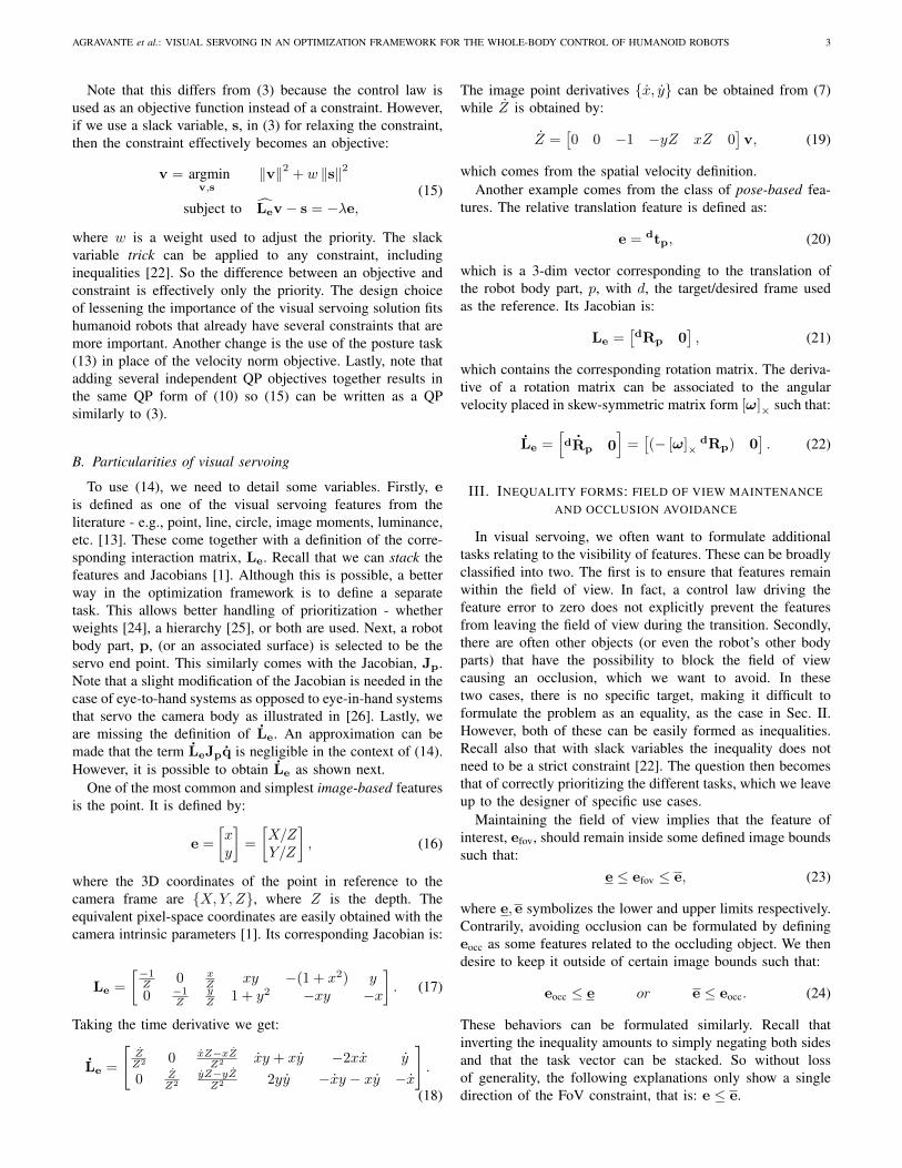
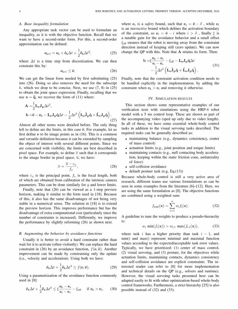
In this simulation, we show how the gaze can be con-trolled simply by centering a single point feature, definedby (16), in the image. Since the feature is defined in imagespace without extrapolating the object pose, the method fallsinto Image-Based Visual Servoing (IBVS). Fig. 1 shows thisdemonstration. The feature is the 2D projection of the user-controlled interactive marker. Additionally, a simulated wallserves as an occluding object to the left of the robot. Forsimplicity, we assume prior knowledge of its location. Todefine the occluding features, the wall edge closest to therobot is sampled with point features. The task limits are theedge of the image border (this is then augmented with thesafety and interactive margins). In the accompanying video,the gaze control motion without occlusion is shown first bymoving the object to the right of the robot. This correspondsto about 3 to 8 sec of the plot in Fig. 2. Contrarily, movingthe object to the left of the robot can result in an occlusionby the wall as seen in Fig. 1. This corresponds to around9 sec onwards of the plot in Fig. 2. The occlusion avoidanceforces the robot to lean forward, noticeably using the torso andleg joints to gaze while maintaining balance (Center of Masscontrol). Additionally note how a small part of the wall entersthe bottom-left corner of the simulated image inset in Fig. 1(gray triangle on the bottom left). This portion is in betweenthe sampled points. Although adding more points can alwaysbe done, it is also possible to use other image features suchas line segments, that can better represent the object.

Fig. 1. A demonstration showing a gazing task using IBVS.

B. Hand servoing with modeling errors

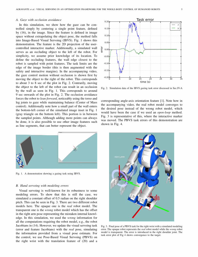
Visual servoing is well-known for its robustness to somemodeling errors. To show that this is still the case, wesimulated a constant offset of 0.5 radian on the right shoulderpitch. This can be seen in Fig. 3. There are two different robotmodels here. The opaque one is the real robot model. Thetransparent one is the wrong robot model which has the offsetin the right arm pose representing the mistaken internal knowl-edge. In this simulation, we used the wrong information forall the computations requiring the robot model, e.g., the robotJacobians in (14). However, we update the visual servoing task(error and feature Jacobians) with the real pose, simulatingthe information provided from a visual pose estimate. Forthe control, we use Pose-Based Visual Servoing (PBVS) onthe right wrist with the translation feature of (20) and a

0 5 10 15 20 25 30 35

time (s)

-0.20

-0.15

-0.10

-0.05

0.00

0.05

0.10

0.15

0.20

err

or

Task error

x

y

Fig. 2. Simulation data of the IBVS gazing task error discussed in Sec.IV-A

corresponding angle-axis orientation feature [1]. Note how inthe accompanying video, the real robot model converges tothe desired pose instead of the wrong robot model, whichwould have been the case if we used an open-loop method.Fig. 3 is representative of this, where the interactive markerwas moved. The PBVS task errors of this demonstration areshown in Fig. 4.

Fig. 3. Final pose of a PBVS task for the right wrist with a simulated modelingerror. The opaque robot represents the real robot model while the wrong robotmodel is transparent. The error is introduced in the right shoulder joint. Thetask error plot of Fig 4 shows convergence to the target.


0 5 10 15 20 25 30 35 40

time (s)

-0.8

-0.6

-0.4

-0.2

0.0

0.2

0.4

0.6

err

or

(t in m

, θu in r

ad)

Task error

tx

ty

tz

θux

θuy

θuz

Fig. 4. Simulation data of the PBVS hand task error discussed in Sec.IV-B,the goal was moved 3 times after initial convergence

C. Combining with walking

Walking (and other locomotion modes) amounts to control-ling the floating base of the humanoid while maintaining bal-ance. This implies that contact states (footsteps) are handled.In this demonstration, we are using a WPG implementationwith a reference velocity as an input [27], [28]. To use thistogether with our visual servoing tasks, a simple but effectivemethod consists of defining the WPG inputs as a functionof the visual servoing task errors. For example, if we have aPBVS task for the right hand and an IBVS gaze task (as in theprevious simulations) then we can define the WPG referenceas:

cxref =kv(txPBVS), cyref =0, θref = −kθ(θgaze),

where the WPG input reference velocities are cxref, cyref, θref,while txPBVS is the translation part of the hand PBVS taskcorresponding to the x axis of the WPG frame (local frame onthe robot), θgaze is the yaw angle of the gaze frame relative tothe current WPG frame and kv, kθ are gains to tune. The ideais that the hand PBVS will guide walking forward. Walkingsideways is not used. The gaze IBVS orients the robot suchthat it faces straight at the object. Finally, note that boundsare needed for txPBVS and θgaze that are used in the coupling.When a bound is exceeded, we use: e′ = e

max(e) where e isthe unbounded error, max(e) is the largest limit violation ande′ is the result used. This preserves the vector direction. Fig. 5shows a screenshot from the demonstration. Fig. 6 shows therelevant WPG control inputs: cxref, θref. The start of the plot ofFig. 6 from time 0 to around 4 sec shows the clipping of thecontrol due to the bound of 0.3 m/s on cxref. After this, up toaround 35 sec, we show how the tasks converged to a fixedgoal. Next, from around 35 sec onwards, we see how the tasksconverged when the interactive goal was moved. Furthermore,there is a small oscillation (especially when the task is close toconverging). This is due to the conflicting tasks (since we arenot using strict hierarchies). Specifically, the visual servoing

task designed in this paper conflicts with the Center of Massservoing with references generated by the WPG. Althoughthe coupling laws designed here seek to resolve this conflict,having a separate solver for the WPG means it cannot be fullyresolved in this manner.

Although this ad hoc coupling is effective in this demon-stration, it has some clear drawbacks. The purpose here was toshow further that visual servoing can be used as just anotherwhole-body task implying that it can work together seamlesslywith balance control and changing contact states. For a morerigorous integration of walking, we think that methods suchas [21] which consider all the conflicting tasks together couldbe a more suitable approach to the problem. However, sincethis requires a larger effort, we have opted to leave this out ofthe scope of this work.

Fig. 5. A demonstration showing walking together with a hand PBVS taskand an IBVS gaze

0 10 20 30 40 50 60 70 80

time (s)

-0.05

0.00

0.05

0.10

0.15

0.20

0.25

0.30

velo

cit

y (

v in m

/s,

˙ θ in r

ad/s

)

WPG control inputs

vx

˙θz

Fig. 6. Simulation data of the walking pattern generator velocity inputscoming from the visual servoing errors discussed in Sec.IV-C

V. TESTS ON A REAL PLATFORM

For validation on a real robot, we are using Romeo, a 37DOF humanoid from SoftBank Robotics. In these tests, weused the left eye camera with a resolution of 320x240 at 30 Hz.


For the interface to Romeo, we used a velocity controller pro-vided by SoftBank Robotics running at 10 Hz. The computedacceleration commands are numerically integrated to providethe required velocity commands.

A. Gaze control with Romeo

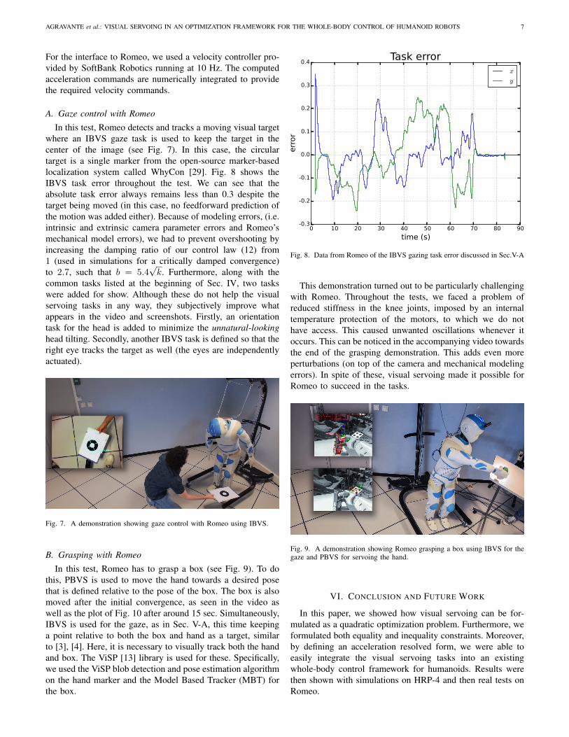
In this test, Romeo detects and tracks a moving visual targetwhere an IBVS gaze task is used to keep the target in thecenter of the image (see Fig. 7). In this case, the circulartarget is a single marker from the open-source marker-basedlocalization system called WhyCon [29]. Fig. 8 shows theIBVS task error throughout the test. We can see that theabsolute task error always remains less than 0.3 despite thetarget being moved (in this case, no feedforward prediction ofthe motion was added either). Because of modeling errors, (i.e.intrinsic and extrinsic camera parameter errors and Romeo’smechanical model errors), we had to prevent overshooting byincreasing the damping ratio of our control law (12) from1 (used in simulations for a critically damped convergence)to 2.7, such that b = 5.4

√k. Furthermore, along with the

common tasks listed at the beginning of Sec. IV, two taskswere added for show. Although these do not help the visualservoing tasks in any way, they subjectively improve whatappears in the video and screenshots. Firstly, an orientationtask for the head is added to minimize the unnatural-lookinghead tilting. Secondly, another IBVS task is defined so that theright eye tracks the target as well (the eyes are independentlyactuated).

Fig. 7. A demonstration showing gaze control with Romeo using IBVS.

B. Grasping with Romeo

In this test, Romeo has to grasp a box (see Fig. 9). To dothis, PBVS is used to move the hand towards a desired posethat is defined relative to the pose of the box. The box is alsomoved after the initial convergence, as seen in the video aswell as the plot of Fig. 10 after around 15 sec. Simultaneously,IBVS is used for the gaze, as in Sec. V-A, this time keepinga point relative to both the box and hand as a target, similarto [3], [4]. Here, it is necessary to visually track both the handand box. The ViSP [13] library is used for these. Specifically,we used the ViSP blob detection and pose estimation algorithmon the hand marker and the Model Based Tracker (MBT) forthe box.

0 10 20 30 40 50 60 70 80 90

time (s)

-0.3

-0.2

-0.1

0.0

0.1

0.2

0.3

0.4

err

or

Task error

x

y

Fig. 8. Data from Romeo of the IBVS gazing task error discussed in Sec.V-A

This demonstration turned out to be particularly challengingwith Romeo. Throughout the tests, we faced a problem ofreduced stiffness in the knee joints, imposed by an internaltemperature protection of the motors, to which we do nothave access. This caused unwanted oscillations whenever itoccurs. This can be noticed in the accompanying video towardsthe end of the grasping demonstration. This adds even moreperturbations (on top of the camera and mechanical modelingerrors). In spite of these, visual servoing made it possible forRomeo to succeed in the tasks.

Fig. 9. A demonstration showing Romeo grasping a box using IBVS for thegaze and PBVS for servoing the hand.

VI. CONCLUSION AND FUTURE WORK

In this paper, we showed how visual servoing can be for-mulated as a quadratic optimization problem. Furthermore, weformulated both equality and inequality constraints. Moreover,by defining an acceleration resolved form, we were able toeasily integrate the visual servoing tasks into an existingwhole-body control framework for humanoids. Results werethen shown with simulations on HRP-4 and then real tests onRomeo.


0 20 40 60 80 100 120

time (s)

-0.4

-0.3

-0.2

-0.1

0.0

0.1

0.2

0.3

0.4

0.5

err

or

(t in m

, θu in r

ad)

Task error

tx

ty

tz

θux

θuy

θuz

Fig. 10. Data from Romeo of the hand PBVS task error discussed in Sec.V-B

For future work, we can envision using the visual servoingtasks in more challenging scenarios. Some specific areas tobe improved in this regard are: the combination with walking,and adding feedforward prediction for target motion tracking.Both of these were briefly outlined here. We also envisionusing other image features and visual constraints to improvethe challenges on real robot platforms such as Romeo.

VII. ACKNOWLEDGEMENT

This work was supported in part by the BPI Romeo 2 andthe H2020 Comanoid projects (www.comanoid.eu).

REFERENCES

[1] F. Chaumette and S. Hutchinson, “Visual servo control, Part I: Basicapproaches,” IEEE Robotics and Automation Magazine, vol. 13, no. 4,pp. 82–90, 2006.

[2] N. Mansard, O. Stasse, F. Chaumette, and K. Yokoi, “Visually-GuidedGrasping while Walking on a Humanoid Robot,” in IEEE InternationalConference on Robotics and Automation, pp. 3041–3047, April 2007.

[3] D. J. Agravante, J. Pages, and F. Chaumette, “Visual servoing for theREEM humanoid robot’s upper body,” in IEEE International Conferenceon Robotics and Automation, pp. 5253–5258, May 2013.

[4] G. Claudio, F. Spindler, and F. Chaumette, “Vision-based manipulationwith the humanoid robot Romeo,” in IEEE-RAS International Confer-ence on Humanoid Robots, pp. 286–293, Nov. 2016.

[5] J. Nocedal and S. Wright, Numerical Optimization. Springer Series inOperations Research and Financial Engineering, Springer New York,2000.

[6] L. Saab, O. E. Ramos, F. Keith, N. Mansard, P. Soueres, and J. Y.Fourquet, “Dynamic Whole-Body Motion Generation Under Rigid Con-tacts and Other Unilateral Constraints,” IEEE Transactions on Robotics,vol. 29, pp. 346–362, April 2013.

[7] J. Koenemann, A. D. Prete, Y. Tassa, E. Todorov, O. Stasse, M. Ben-newitz, and N. Mansard, “Whole-body model-predictive control appliedto the HRP-2 humanoid,” in IEEE/RSJ International Conference onIntelligent Robots and Systems, pp. 3346–3351, Sept 2015.

[8] J. Vaillant, A. Kheddar, H. Audren, F. Keith, S. Brossette, A. Escande,K. Bouyarmane, K. Kaneko, M. Morisawa, P. Gergondet, E. Yoshida,S. Kajita, and F. Kanehiro, “Multi-contact vertical ladder climbing withan HRP-2 humanoid,” Autonomous Robots, vol. 40, no. 3, pp. 561–580,2016.

[9] A. Herzog, N. Rotella, S. Mason, F. Grimminger, S. Schaal, andL. Righetti, “Momentum control with hierarchical inverse dynamicson a torque-controlled humanoid,” Autonomous Robots, vol. 40, no. 3,pp. 473–491, 2015.

[10] S. Kuindersma, R. Deits, M. Fallon, A. Valenzuela, H. Dai, F. Permenter,T. Koolen, P. Marion, and R. Tedrake, “Optimization-based locomotionplanning, estimation, and control design for the atlas humanoid robot,”Autonomous Robots, vol. 40, no. 3, pp. 429–455, 2016.

[11] M. Johnson, B. Shrewsbury, S. Bertrand, T. Wu, D. Duran, M. Floyd,P. Abeles, D. Stephen, N. Mertins, A. Lesman, J. Carff, W. Rifenburgh,P. Kaveti, W. Straatman, J. Smith, M. Griffioen, B. Layton, T. de Boer,T. Koolen, P. Neuhaus, and J. Pratt, “Team IHMC’s Lessons Learnedfrom the DARPA Robotics Challenge Trials,” Journal of Field Robotics,vol. 32, no. 2, pp. 192–208, 2015.

[12] S. Feng, E. Whitman, X. Xinjilefu, and C. G. Atkeson, “Optimization-based Full Body Control for the DARPA Robotics Challenge,” Journalof Field Robotics, vol. 32, no. 2, pp. 293–312, 2015.

[13] E. Marchand, F. Spindler, and F. Chaumette, “ViSP for visual servoing:a generic software platform with a wide class of robot control skills,”IEEE Robotics and Automation Magazine, vol. 12, no. 4, pp. 40–52,2005.

[14] Y. Mezouar and F. Chaumette, “Path planning for robust image-basedcontrol,” IEEE Transactions on Robotics and Automation, vol. 18,pp. 534–549, Aug 2002.

[15] A. H. A. Hafez, A. K. Nelakanti, and C. V. Jawahar, “Path planningapproach to visual servoing with feature visibility constraints: A convexoptimization based solution,” in IEEE/RSJ International Conference onIntelligent Robots and Systems, pp. 1981–1986, Oct 2007.

[16] T. Shen and G. Chesi, “Visual Servoing Path Planning for CamerasObeying the Unified Model,” Advanced Robotics, vol. 26, no. 8-9,pp. 843–860, 2012.

[17] M. Kazemi, K. K. Gupta, and M. Mehrandezh, “Randomized Kino-dynamic Planning for Robust Visual Servoing,” IEEE Transactions onRobotics, vol. 29, pp. 1197–1211, Oct 2013.

[18] G. Allibert, E. Courtial, and F. Chaumette, “Predictive Control for Con-strained Image-Based Visual Servoing,” IEEE Transactions on Robotics,vol. 26, pp. 933–939, Oct 2010.

[19] M. Garcia, O. Stasse, J.-B. Hayet, C. Dune, C. Esteves, and J.-P. Laumond, “Vision-guided motion primitives for humanoid reactivewalking: Decoupled versus coupled approaches,” International Journalof Robotics Research, vol. 34, no. 4-5, pp. 402–419, 2015.

[20] S. Kajita, M. Morisawa, K. Miura, S. Nakaoka, K. Harada, K. Kaneko,F. Kanehiro, and K. Yokoi, “Biped walking stabilization based on linearinverted pendulum tracking,” in IEEE/RSJ International Conference onIntelligent Robots and Systems, pp. 4489–4496, Oct 2010.

[21] A. Sherikov, D. Dimitrov, and P.-B. Wieber, “Whole body motion con-troller with long-term balance constraints,” in IEEE-RAS InternationalConference on Humanoid Robots, pp. 444–450, Nov 2014.

[22] O. Kanoun, F. Lamiraux, and P. B. Wieber, “Kinematic Control ofRedundant Manipulators: Generalizing the Task-Priority Framework toInequality Task,” IEEE Transactions on Robotics, vol. 27, pp. 785–792,Aug 2011.

[23] E. Malis, “Improving vision-based control using efficient second-orderminimization techniques,” in IEEE International Conference on Roboticsand Automation, vol. 2, pp. 1843–1848 Vol.2, April 2004.

[24] K. Bouyarmane and A. Kheddar, “Using a multi-objective controllerto synthesize simulated humanoid robot motion with changing contactconfigurations,” in IEEE/RSJ International Conference on IntelligentRobots and Systems, pp. 4414–4419, Sept 2011.

[25] A. Escande, N. Mansard, and P.-B. Wieber, “Hierarchical quadraticprogramming: Fast online humanoid-robot motion generation,” TheInternational Journal of Robotics Research, 2014.

[26] F. Chaumette and S. Hutchinson, “Visual servo control, Part II: Ad-vanced approaches,” IEEE Robotics and Automation Magazine, vol. 14,no. 1, pp. 109–118, 2007.

[27] D. J. Agravante, A. Sherikov, P. B. Wieber, A. Cherubini, and A. Khed-dar, “Walking pattern generators designed for physical collaboration,” inIEEE International Conference on Robotics and Automation, pp. 1573–1578, May 2016.

[28] A. Herdt, H. Diedam, P.-B. Wieber, D. Dimitrov, K. Mombaur, andM. Diehl, “Online walking motion generation with automatic footstepplacement,” Advanced Robotics, vol. 24, no. 5-6, pp. 719–737, 2010.

[29] T. Krajnık, M. Nitsche, J. Faigl, P. Vanek, M. Saska, L. Preucil,T. Duckett, and M. Mejail, “A Practical Multirobot Localization Sys-tem,” Journal of Intelligent & Robotic Systems, vol. 76, no. 3, pp. 539–562, 2014.

visual servoing in an optimization framework for the whole ... · agravante et al. : visual...

Documents