visualization, identification, and estimation in the linear
TRANSCRIPT
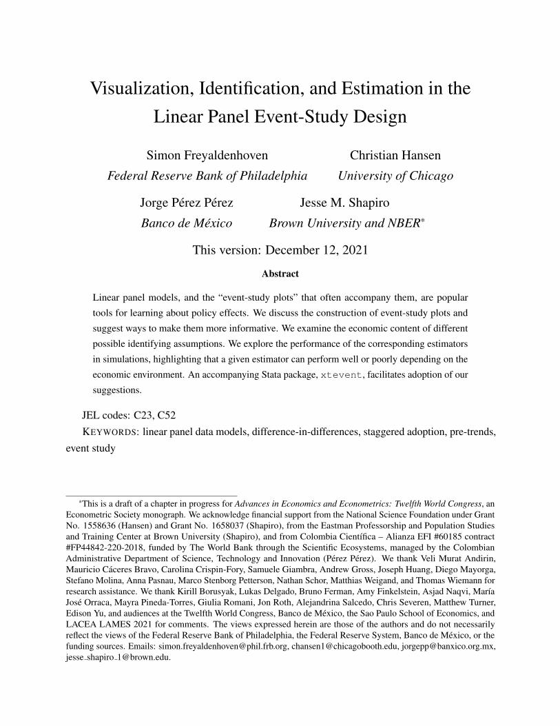
Visualization, Identification, and Estimation in theLinear Panel Event-Study Design
Simon Freyaldenhoven
Federal Reserve Bank of Philadelphia
Christian Hansen
University of Chicago
Jorge Perez Perez
Banco de Mexico
Jesse M. Shapiro
Brown University and NBER*
This version: December 12, 2021
Abstract
Linear panel models, and the “event-study plots” that often accompany them, are popular
tools for learning about policy effects. We discuss the construction of event-study plots and
suggest ways to make them more informative. We examine the economic content of different
possible identifying assumptions. We explore the performance of the corresponding estimators
in simulations, highlighting that a given estimator can perform well or poorly depending on the
economic environment. An accompanying Stata package, xtevent, facilitates adoption of our
suggestions.
JEL codes: C23, C52KEYWORDS: linear panel data models, difference-in-differences, staggered adoption, pre-trends,
event study
*This is a draft of a chapter in progress for Advances in Economics and Econometrics: Twelfth World Congress, anEconometric Society monograph. We acknowledge financial support from the National Science Foundation under GrantNo. 1558636 (Hansen) and Grant No. 1658037 (Shapiro), from the Eastman Professorship and Population Studiesand Training Center at Brown University (Shapiro), and from Colombia Cientıfica – Alianza EFI #60185 contract#FP44842-220-2018, funded by The World Bank through the Scientific Ecosystems, managed by the ColombianAdministrative Department of Science, Technology and Innovation (Perez Perez). We thank Veli Murat Andirin,Mauricio Caceres Bravo, Carolina Crispin-Fory, Samuele Giambra, Andrew Gross, Joseph Huang, Diego Mayorga,Stefano Molina, Anna Pasnau, Marco Stenborg Petterson, Nathan Schor, Matthias Weigand, and Thomas Wiemann forresearch assistance. We thank Kirill Borusyak, Lukas Delgado, Bruno Ferman, Amy Finkelstein, Asjad Naqvi, MarıaJose Orraca, Mayra Pineda-Torres, Giulia Romani, Jon Roth, Alejandrina Salcedo, Chris Severen, Matthew Turner,Edison Yu, and audiences at the Twelfth World Congress, Banco de Mexico, the Sao Paulo School of Economics, andLACEA LAMES 2021 for comments. The views expressed herein are those of the authors and do not necessarilyreflect the views of the Federal Reserve Bank of Philadelphia, the Federal Reserve System, Banco de Mexico, or thefunding sources. Emails: [email protected], [email protected], [email protected],jesse shapiro [email protected].

1 Introduction
A common situation in empirical economics is one where we are interested in learning the dynamiceffect of a scalar policy zit on some outcome yit in an observational panel of units i ∈ {1, ..., N}observed in a sequence of periods t ∈ {1, ..., T}. Examples include
• the effect of participation in a training program (e.g., Ashenfelter 1978), where units i areindividuals, the policy variable zit is an indicator for program participation, and the outcomeyit is earnings;
• the effect of the minimum wage (e.g., Brown 1999), where units i are US states, the policyvariable zit is the level of the minimum wage, and the outcome yit is the employment rate ofsome group; and
• the effect of Walmart (e.g., Basker 2005), where units i are cities, the policy variable zit is anindicator for the presence of a Walmart, and the outcome yit is a measure of retail prices.
A common model for representing this situation is a linear panel model with dynamic policyeffects:
yit = αi + γt + q′itψ +M∑
m=−G
βmzi,t−m + Cit + εit, (1)
Here, αi denotes a unit fixed effect, γt a time fixed effect, and qit a vector of controls withconformable coefficients ψ. The scalar Cit denotes a (potentially unobserved) confound that maybe correlated with the policy, and the scalar εit represents an unobserved shock that is not correlatedwith the policy. Estimates of models of the form in (1) are common in economic applications.1
The term∑M
m=−G βmzi,t−m means that the policy can have dynamic effects. The outcome attime t can only be directly affected by the value of the policy at most M ≥ 0 periods before t andat most G ≥ 0 periods after t. The values of G and M are often assumed by the researcher. Theparameters {βm}Mm=−G summarize the magnitude of the dynamic effects and are often estimated.Estimates of {βm}Mm=−G are often summarized in an “event-study plot” of the form in Figure 1,which we may loosely think of as depicting estimates of the cumulative effects
∑km=−G βm at
different horizons k.2
1Freyaldenhoven et al. (2019) identify 16 articles using a linear panel model in the 2016 issues of the AmericanEconomic Review. During the July 2020 meeting of the NBER Labor Studies Program, estimates of a model of theform in (1) played an important role in at least one presentation on three of the four meeting dates. See Aghion et al.(2020), Ayromloo et al. (2020), and Derenoncourt et al. (2020).
2Roth (2021) identifies 70 papers published in three American Economic Association journals between 2014 and June2018 that include such a plot.
1

−.2
0
.2
.4
.6
Co
eff
icie
nt
−6+ −5 −4 −3 −2 −1 0 1 2 3 4 5+
Event time
Figure 1: Exemplary event-study plot. The plot shows a hypothetical example of an event-study plot. SeeSection 2 for details on the construction of event-study plots.
In economic settings, variation in the policy may be related to other determinants of the outcome.For example, a person’s entry into a training program may reflect unobserved shocks to earnings, astate’s decision to increase its minimum wage may be influenced by its economic performance, andWalmart’s arrival in a city may signal trends in the local retail environment. Such factors make itchallenging to identify {βm}Mm=−G, and are captured in (1) via the confound Cit. If the confoundis unobserved, identification of {βm}Mm=−G typically requires substantive restrictions on Cit thatcannot be learned entirely from the data and must therefore be justified on economic grounds.
In this chapter, we have three main goals. The first, which we take up in Section 2, is to makesuggestions on the construction of event-study plots of the form in Figure 1. These suggestionsaim at improving the informativeness of these plots. They involve a mix of codifying what weconsider common best practices, as well as suggesting some practices that are not currently in use.An accompanying Stata package, xtevent, makes it easier for readers to adopt our suggestions.
The second, which we take up in Section 3, is to consider possible approaches to identification of{βm}Mm=−G. Each approach requires some restrictions on the confound Cit. In accordance with ourview that such restrictions should be motivated on economic grounds, our discussion emphasizesand contrasts the economic content of different possible restrictions.
The third, which we take up in Section 4 and an accompanying Appendix, is to illustrate theperformance of different estimators under some specific data-generating processes. We choose data-generating processes motivated by the economic settings of interest, and estimators correspondingto the approaches to identification that we discuss in Section 3. Our simulations highlight thatthere is not one “best” estimator—a given estimator may perform well or poorly depending on theunderlying economic environment. The simulation results reinforce the importance of matchingidentifying assumptions (and the corresponding estimator) to the setting at hand.
2

The model in (1) is flexible in some respects. It allows the policy to have dynamic effects beforeand after its contemporaneous value. Additionally it does not restrict the form of zit, which may inprinciple be continuous, discrete, or binary. One important case, referenced in the literature andthroughout our discussion, is that of staggered adoption, in which the policy is binary, zit ∈ {0, 1};all units begin without the policy, zi1 = 0 for all i; and once the policy is adopted by a given unit itis never reversed, zit′ ≥ zit for all i and t′ ≥ t.3
The model in (1) is also restrictive in many respects. It assumes that all terms enter in alinear, separable way.4 It includes neither lagged dependent variables nor predetermined variables.The model in (1) also assumes that the effect of the policy is homogeneous across units i. Anactive literature explores the implications of relaxing this homogeneity.5 Although we maintainhomogeneity throughout most of the exposition, we discuss in Section 3 how to adapt the approachesto identification we consider there to allow for some forms of heterogeneous policy effects, andwe illustrate in Section 4 how to estimate policy effects in the presence of both heterogeneity andconfounding. An important theme of our discussion is that accounting for heterogeneity in policyeffects is not a substitute for accounting for confounding, and vice versa.
2 Plotting
For this section, we assume the researcher has adopted assumptions sufficient for the identificationand estimation of {βm}Mm=−G, and consider how to plot the resulting estimates for the reader. Wereturn to the question of how to obtain such estimates in later sections. Thus, we do not explicitlyconsider specific restrictions on the confound Cit in this section, but we emphasize that all of theapproaches to restricting the confound that we discuss in Section 3, and all of the correspondingestimators that we employ in Section 4, can be applied in tandem with the approaches to plottingthat we develop in this section.
2.1 The Basics
There are two important ways in which a typical event-study plot departs from a plot of theestimates of {βm}Mm=−G in (1). The first is that, for visual reasons, it is often appealing to depictcumulative estimated effects of the policy. To simplify estimating cumulative effects, we adopt arepresentation of (1) in terms of changes in the policy zit. The second is that, to permit visualizationof overidentifying information, it is often appealing to plot cumulative estimated effects of the
3See, for example, Shaikh and Toulis (2021), Ben-Michael et al. (2021), and Athey and Imbens (forthcoming).4Athey and Imbens (2006) and Roth and Sant’Anna (2021), among others, consider nonlinear models in the canonicaldifference-in-differences setting.
5See, for example, de Chaisemartin and D’Haultfoeuille (2020), Athey and Imbens (forthcoming), Goodman-Bacon(2021), Callaway and Sant’Anna (2021), and Sun and Abraham (2021).
3

policy at horizons outside of the range of horizons over which the policy is thought to affect theoutcome. To make it possible to include such estimates on the plot, we generalize (1) to entertainthat a change in the policy at time t leads to a change in the outcome LG ≥ 0 periods before t−G
and LM ≥ 0 periods after t+M .Specifically, we estimate the following regression model:
yit =
M+LM−1∑k=−G−LG
δk∆zi,t−k + δM+LMzi,t−M−LM
+ δ−G−LG−1(1− zi,t+G+LG)
+ αi + γt + q′itψ + Cit + εit,
(2)
where ∆ denotes the first difference operator. To build intuition for the form of (2), note that inthe special case of staggered adoption, ∆zi,t−k is an indicator for whether unit i adopted the policyexactly k periods before period t, zi,t−M−LM
is an indicator for whether unit i adopted at leastM + LM periods before period t, and (1− zi,t+G+LG
) is an indicator for whether unit i will adoptmore than G+ LG periods after period t.
The parameters {δk}k=M+LMk=−G−LG−1 can be interpreted as cumulative policy effects at different
horizons. In particular, (1) implies that
δk =
0 for k < −G∑k
m=−G βm for −G ≤ k ≤M∑Mm=−G βm for k > M.
(3)
See, for example, Schmidheiny and Siegloch (2020) and Sun and Abraham (2021). The rep-resentation in (3) holds for general forms of the policy zit, not only for the case of staggeredadoption.
The core of an event-study plot, illustrated by Figure 1, is a plot of the points
{(k, δk)}k=M+LMk=−G−LG−1,
where {δk}k=M+LMk=−G−LG−1 are the estimates of {δk}k=M+LM
k=−G−LG−1. We refer to k as event time, to thevector δ = (δ−G−LG−1, ..., δM+LM
)′ as the event-time path of the outcome variable, and to thecorresponding estimate δ as the estimated event-time path of the outcome variable. In the case ofstaggered adoption, the “event” is the adoption of the policy. Recall, however, that we allow formore general forms of the policy zit, including that it exhibits multiple changes or “events,” or thatit is continuous. We include a + symbol in the x-axis label for event times k = −G− LG − 1 andk =M + LM as a reminder of the interpretation of the corresponding terms in (2).
4

−1.5
−.8
0
.8
1.5C
oeffic
ient
−6+ −5 −4 −3 −2 −1 0 1 2 3 4 5 6+
Event time
(a) “Smooth” event-time trend
−1.5
−.8
0
.8
1.5
Coeffic
ient
−6+ −5 −4 −3 −2 −1 0 1 2 3 4 5 6+
Event time
(b) “Jump” at the time of the event
Figure 2: Baseline event-study plot. Exemplary event-study plot for two possible datasets. Each plot depictsthe elements of the estimated event-time path of the outcome, δk, on the y-axis, against event time, k, on thex-axis. The intervals are pointwise 95 percent confidence intervals for the corresponding elements, δk, of theevent-time path of the outcome. In the left panel the estimated event-time path of the outcome is “smooth.”In the right panel the estimated event-time path of the outcome exhibits a “jump” at the time of the event.The value of δ−1 has been normalized to 0, in accordance with Suggestion 1.
2.2 Normalization
The event-study plot is meant to illustrate the cumulative effect of the policy on the outcome. Theeffect of the policy must be measured with reference to some baseline. This manifests in (2) throughthe fact that the policy variables in the equation are collinear (they sum to zero), meaning that anormalization is required for identification of the event-time path. Indeed, one reason it is valuableto include the endpoint variables zi,t+G+LG
and zi,t−M−LMin (2) is that, by saturating the model,
inclusion of these variables forces a conscious choice of normalization.A common choice of normalization, and one that we think serves as a good default, is δ−G−1 = 0.
In the leading case where G = 0, i.e., future values of the policy cannot affect the current value ofthe outcome, this default implies a normalization δ−1 = 0. In the case of staggered adoption, thenormalization δ−1 = 0 means that the plotted coefficients can be interpreted as estimated effectsrelative to the period before adoption. More generally, the normalization δ−1 = 0 means that theplotted coefficients can be interpreted as estimated effects relative to the effect of a one-unit changein the policy variable one period ahead.
Suggestion 1. Normalize δ−G−1 = 0 when estimating (2).
Figure 2 illustrates an event-study plot with the normalization δ−1 = 0 for two possible datasets.Both figures exhibit identical pre-event dynamics. After event time −1, Figure 2(a) exhibits a“smooth” continuation of pre-event trends, whereas Figure 2(b) exhibits a “jump.” The figureincludes pointwise 95 percent confidence intervals for the elements of the event-time path. The
5

normalization δ−1 = 0 makes it easy to use the depicted confidence intervals to test the pointhypothesis that the event-time path is identical at event times −1 and k, i.e., H0 : δ−1 = δk. Forexample, setting k = 0, a reader of Figure 2(a) can readily conclude that there is no statisticallysignificant change in the outcome at event time 0. A reader of Figure 2(b) can readily conclude thatthere is a statistically significant change in the outcome at event time 0.
2.3 Magnitude
A given cumulative effect of the policy can have a different interpretation depending on the baselinelevel of the dependent variable. To make it easier for a reader to evaluate economic significance, wesuggest to include a parenthetical label for the normalized coefficient δk∗ that conveys a referencevalue for the outcome.
Suggestion 2. Include a parenthetical label for the normalized coefficient δk∗ that has value∑(i,t):∆zi,t−k∗ =0 yit
|(i, t) : ∆zi,t−k∗ = 0|. (4)
The value in (4) corresponds to the mean of the dependent variable (−k∗) periods in advance of apolicy change.6 For example, if G = 0, then following Suggestion 1 we would normalize δ−1 = 0,and following Suggestion 2 we would include a parenthetical label with value
∑(i,t):∆zi,t+1 =0 yit
|(i,t):∆zi,t+1 =0| . Inthe special case of staggered adoption, this expression corresponds to the sample mean of yit oneperiod before adoption. More generally, it corresponds to the sample mean of yit one period beforea policy change.
Figure 3 illustrates Suggestion 2 by adding the proposed parenthetical label next to the 0 pointon the y-axis. The parenthetical label makes it easier to interpret the magnitude of the estimatedcumulative policy effects depicted on the plot. For example, in Figure 3(a), the coefficient estimateδ3 implies that the estimated cumulative effect of the policy on the outcome at event time 3, measuredrelative to event time −1, is roughly -0.73. This effect appears to be modest relative to 41.94, thesample mean of the dependent variable one period in advance of a policy change, shown in theparenthetical label.
2.4 Inference
It is common for researchers to include 95 percent pointwise confidence intervals for the elementsof the event-time path, as we have done in Figures 1 through 3. As we discuss in Section 2.2, theseconfidence intervals make it easy for a reader to answer prespecified statistical questions about thevalue of an individual element of the event-time path, relative to that of the normalized element.6When multiple coefficients in δ are normalized, we propose to label the value of the one whose index is closest to zero.
6

−1.5
−.8
0 (41.94)
.8
1.5C
oeffic
ient
−6+ −5 −4 −3 −2 −1 0 1 2 3 4 5 6+Event time
(a) “Smooth” event-time trend
−1.5
−.8
0 (41.94)
.8
1.5
Coeffic
ient
−6+ −5 −4 −3 −2 −1 0 1 2 3 4 5 6+Event time
(b) “Jump” at the time of the event
Figure 3: Label for normalized coefficient. Exemplary event-study plot for two possible datasets. Relativeto Figure 2, a parenthetical label for the average value of the outcome corresponding to the normalizedcoefficient has been added, in accordance with Suggestion 2.
A reader may also be interested in answering statistical questions about the entire event-timepath, rather than merely a single element. Because such questions involve multiple parametersand will typically not be prespecified, answering them reliably requires accounting for the factthat the reader is implicitly testing multiple hypotheses at once. A convenient way to do this is toaugment the plot by adding a 95 percent uniform confidence band. Just as a 95 percent pointwiseconfidence interval is designed to contain the true value of an individual parameter at least 95percent of the time, a 95 percent uniform confidence band is designed to contain the true value of aset of parameters at least 95 percent of the time.
We specifically suggest plotting a sup-t confidence band. A sup-t band is straightforward tovisualize in an event-study plot and can be computed fairly easily in the settings we consider byusing draws from the estimated asymptotic distribution of δ to compute a critical value. Interestedreaders may see, for example, Freyberger and Rai (2018) or Olea and Plagborg-Møller (2019) fordetails.
Suggestion 3. Plot a uniform sup-t confidence band for the event-time path of the outcome δ, in
addition to pointwise confidence intervals for the individual elements of the event-time path.
Figure 4 illustrates Suggestion 3 by adding a set of outer lines comprising the sup-t band tothe plots in Figure 3, retaining the pointwise confidence intervals as the inner bars. Just as anyvalue of an element of the event-time path that lies outside the inner confidence interval can beregarded as statistically inconsistent with the corresponding estimate, any event-time path that doesnot pass entirely within the outer confidence band can be regarded as statistically inconsistent withthe estimated path. For example, in both plots, we cannot reject the hypothesis that the event-timepath is equal to zero in all pre-event periods using the uniform confidence bands. On the other
7

−1.5
−.8
0 (41.94)
.8
1.5C
oeffic
ient
−6+ −5 −4 −3 −2 −1 0 1 2 3 4 5 6+Event time
(a) “Smooth” event-time trend
−1.5
−.8
0 (41.94)
.8
1.5
Coeffic
ient
−6+ −5 −4 −3 −2 −1 0 1 2 3 4 5 6+Event time
(b) “Jump” at the time of the event
Figure 4: Uniform confidence band. Exemplary event-study plot for two possible datasets. Relative toFigure 3, uniform confidence bands have been added, in accordance with Suggestion 3. The pointwiseconfidence intervals are illustrated by the inner bars, and the uniform, sup-t confidence bands are given by theouter lines.
hand, we would conclude that δ−5 is statistically significant using the pointwise intervals. Unlesswe had prespecified that we were specifically interested in the null hypothesis that δ−5 = 0, the firstconclusion based on the uniform confidence bands appears more suitable.
2.5 Overidentification and Testing
The model in (1) asserts that changes in the policy variable more than G periods in the future donot change the outcome. Taking LG > 0 and thus including event times earlier than −G in theplot means that the plot contains information about whether this hypothesis is consistent with thedata. A failure of this hypothesis might indicate anticipatory behavior, or, in what seems a morecommon interpretation in practice, it might indicate the presence of a confound. Because in manysituations G = 0, researchers sometimes refer to a test of this hypothesis as a test for pre-eventtrends or “pre-trends.”
The model in (1) also asserts that changes in the policy variable more than M periods in thepast do not change the outcome. Taking LM > 0 and thus including event times after M in the plotmeans that the plot contains information about whether this hypothesis is consistent with the data.A failure of this hypothesis might indicate richer dynamic effects of the policy than the researcherhas contemplated.
Each of these hypotheses can be tested formally via a Wald test. The result of the Wald testcannot generally be inferred from the pointwise confidence intervals or uniform confidence band.We therefore propose to include the p-values corresponding to each of the two Wald tests.
8

−1.5
−.8
0 (41.94)
.8
1.5C
oeffic
ient
−6+ −5 −4 −3 −2 −1 0 1 2 3 4 5 6+Event time
Pretrends p−value = 0.22 −− Leveling off p−value = 0.76
(a) “Smooth” event-time trend
−1.5
−.8
0 (41.94)
.8
1.5
Coeffic
ient
−6+ −5 −4 −3 −2 −1 0 1 2 3 4 5 6+Event time
Pretrends p−value = 0.22 −− Leveling off p−value = 0.76
(b) “Jump” at the time of the event
Figure 5: Testing p-values. Exemplary event-study plot for two possible datasets. Relative to Figure 4,p-values for testing for the absence of pre-event effects and p-values for testing the null that dynamics haveleveled off have been added, in accordance with Suggestion 4.
Suggestion 4. Include in the plot legend p-values for Wald tests of each of the following hypotheses:
H0 : δk = 0, −G− LG − 1 ≤ k < −G (no pre-trends)
H0 : δM = δM+k, 0 < k ≤ LM (dynamics level off)
Figure 5 illustrates Suggestion 4 by adding the two suggested p-values to the plots from Figure4, taking G = 0 and LM = 1. In both cases, the tested hypotheses are not rejected at conventionallevels.
The exact specification of the hypotheses listed in Suggestion 4 depends on the choice of LG
and LM . Formally, these control the number of overidentifying restrictions that (1) imposes on (2).We do not offer a formal procedure for choosing LG and LM . Instead, we suggest a default rule ofthumb that we expect will be reasonable in many cases.
Suggestion 5. Set LM = 1 and set LG =M +G.
Setting LM = 1 guarantees that it is possible to test the researcher’s hypothesis that changes inthe policy variable more thanM periods in the past do not change the outcome. Setting LG =M+G
makes the plot “symmetric,” in the sense that it permits testing for pre-trends over as long of ahorizon as the policy is thought to affect the outcome. If we take M = 5 and G = 0, then Figure 5is consistent with Suggestion 5.
2.6 Confounds
A failure to reject the hypothesis of no pre-trends does not mean there is no confound, or eventhat there are no pre-trends (Roth 2021). Any estimated event-time path for the outcome can be
9

reconciled with a devil’s-advocate model in which the policy has no effect on the outcome, i.e., inwhich the true values of {βm}Mm=−G are zero. In this devil’s-advocate model, all of the dynamics ofthe estimated event-time path of the outcome variable are driven by an unmeasured confound.
In some cases, the sort of confound needed to fully explain the event-time path of the outcomemay be economically implausible. To help the reader evaluate the plausibility of the confoundsthat are consistent with the data, we propose to add to the event-study plot a representation of the“most plausible” confound that is statistically consistent with the estimated event-time path of theoutcome. There is no universal notion of what is plausible, but we expect that in many situations,less “wiggly” confounds will be more plausible than more “wiggly” ones.
Among polynomial confounds that are consistent with the estimated event-time path of theoutcome, we propose to define the least “wiggly” one as the one that has the lowest possiblepolynomial order and that, among polynomials with that order, has the coefficient with lowestpossible magnitude on its highest-order term. Towards a formalization, for v a finite-dimensionalcoefficient vector and k an integer, define the polynomial term δ∗k(v) =
∑dim(v)j=1 vjk
j−1, where vjdenotes the j th element of coefficient vector v and dim(v) denotes the dimension of this vector.Let δ∗(v) collect the elements δ∗k(v) for −G − LG − 1 ≤ k ≤ M + LM , so that δ∗(v) reflects apolynomial path in event time with coefficients v.
Suggestion 6. Plot the least “wiggly” confound whose path is contained in the Wald region CR(δ)
for the event-time path of the outcome. Specifically, plot δ∗(v∗), where
p∗ = min{dim(v) : δ∗(v) ∈ CR(δ)} and (5)
v∗ = argminv
{v2p∗ : dim(v) = p∗, δ∗(v) ∈ CR(δ)}. (6)
This suggestion is closely related to the sensitivity analysis proposed in Rambachan and Roth(2021).
Figure 6 illustrates Suggestion 6 by adding the path δ∗(v∗) to the plot in Figure 5. In Figure6(a), the estimated event-time path is consistent with a confound that follows a very “smooth” path,close to linear in event time, that begins pre-event and simply continues post-event. We suspect thatin many economic settings such confound dynamics would be considered plausible, thus suggestingthat a confound can plausibly explain the entire event-time path of the outcome, and therefore thatthe policy might plausibly have no effect on the outcome.
In Figure 6(b), by contrast, the estimated event-time path demands a confound with a very“wiggly” path. We suspect that in many economic settings such confound dynamics would not beconsidered plausible, thus suggesting that a confound cannot plausibly explain the entire event-timepath of the outcome, and therefore that the policy does affect the outcome.
10

−1.5
−.8
0 (41.94)
.8
1.5C
oeffic
ient
−6+ −5 −4 −3 −2 −1 0 1 2 3 4 5 6+Event time
Pretrends p−value = 0.22 −− Leveling off p−value = 0.76
(a) “Smooth” event-time trend
−1.5
−.8
0 (41.94)
.8
1.5
Coeffic
ient
−6+ −5 −4 −3 −2 −1 0 1 2 3 4 5 6+Event time
Pretrends p−value = 0.22 −− Leveling off p−value = 0.76
(b) “Jump” at the time of the event
Figure 6: Least “wiggly” path of confound. Exemplary event-study plot for two possible datasets. Relativeto Figure 5, a curve has been added that illustrates the least “wiggly” confound that is consistent with theevent-time path of the outcome, in accordance with Suggestion 6.
2.7 Summarizing Policy Effects
Researchers sometimes present a scalar summary of the magnitude of the policy effect. One wayto obtain such a summary is to compute an average or other scalar function of the post-eventeffects depicted in the plot (de Chaisemartin and D’Haultfoeuille 2021). Another is to estimate astatic version of (1) including only the contemporaneous value of the policy variable (restrictingM = G = 0 as in, e.g., Gentzkow et al. 2011). In the case where the researcher imposes this (orsome other) restriction, we suggest to evaluate the fit of the more restrictive model to the dynamicsof a more flexible model that allows for dynamic effects, such as (2), as follows.
Suggestion 7. If using a more restrictive model than (1) to summarize magnitude, visualize the
implied restrictions as follows:
1. Estimate (1) subject to the contemplated restrictions.
2. Use (3) to translate the estimates from (1) into cumulative effects.
3. Overlay the estimated cumulative effects on the event-study plot.
Figure 7 illustrates this suggestion in a hypothetical example in which the more restrictive modelassumes that the policy effect is static, i.e., that the current value of the policy affects only thecurrent value of the outcome. Comparison of the two event-time paths provides a visualization ofthe fit of the more restrictive model. The uniform confidence band permits visual assessment of themore restrictive model. In the case shown in Figure 7, the more restrictive model is not included inthe uniform confidence band, implying that we can reject the hypothesis that the effect of the policyis static. Figure 7 also displays the p-value from a Wald test of the more restrictive model, which
11

−.5
.5
1
1.5
0 (5.12)
Co
eff
icie
nt
−6+ −5 −4 −3 −2 −1 0 1 2 3 4 5 6+Event time
Constant effects p−value = 0.00
Figure 7: Evaluating the fit of a more restrictive model. Here, we overlay estimates from a model thatimposes static treatment effects with estimates from a more flexible model that allows for dynamic treatmenteffects, in accordance with Suggestion 7.
also implies that the more restrictive model is rejected. The Wald test may be more powerful fortesting this joint hypothesis than the test based on the sup-t band, but its implications are harder tovisualize in this setting (Olea and Plagborg-Møller 2019).
3 Approaches to Identification
We now discuss approaches to identification of the parameters {βm}Mm=−G in (1), which for easeof reference we collect in a vector β. Since, in general, the confound Cit will not be observed,identification of β will rely on restrictions on how observable and latent variables relate to Cit andzit. To simplify statements, we decompose the confound Cit into a component that depends on a low-dimensional set of time-varying factors with individual-specific coefficients, and an idiosyncraticcomponent such that
Cit = λ′iFt + ξηit, and thus (7)
yit = αi + γt + q′itψ +M∑
m=−G
βmzi,t−m + λ′iFt + ξηit + εit. (8)
In (7) and (8), Ft is a vector of (possibly unobserved) factors with (possibly unknown) unit-specificloadings λi, and ηit is an unobserved scalar with (possibly unknown) coefficient ξ.
We assume that G and M are known. In some settings it may be possible to estimate M , thoughinference on β would then need to account for data-driven choice of M . In some settings it mayalso be possible to estimate G, but because pre-trends are often used to diagnose confounding,we instead suggest choosing G on economic grounds. See Schmidheiny and Siegloch (2020) and
12

Borusyak et al. (2021a) for related discussion.To formalize the sense in which Cit is a confound, we maintain throughout that
E[εit|F, λi, ηi, zi, αi, γ, qi] = 0, (9)
with F , ηi, zi, γ, and qi collecting all T observations of Ft, ηit, zit, γt, and qit, respectively. Giventhis condition, if the factor Ft and the scalar ηit were observed, then with sufficiently rich data itwould be possible to identify β simply by treating Ft and ηit as control variables. If Ft and ηit arenot observed, then in general β is not identified.
Intuitively, then, identification of β will require restrictions on Ft and ηit. Typically theappropriate identifying assumptions cannot be learned from the data and so should ideally bejustified on economic grounds. Our discussion therefore emphasizes and contrasts the economiccontent of different assumptions. We mostly focus on situations where only one of Ft or ηit isrelevant, but in principle it seems possible to “mix and match” approaches when both componentsmay be present.
3.1 Not Requiring Proxies or Instruments
The first class of approaches imposes sufficient structure on how latent variables enter the model sothat the parameters β can be identified without the use of proxy or instrumental variables. We beginwith a situation where the confound is low-dimensional (ξ = 0).
Assumption 1. ξ = 0 and one of the following holds:
(a) Ft = 0 for all t.
(b) Ft = f(t) for f(·) a known low-dimensional set of basis functions.
(c) The dimension of Ft is small.
Note that although we state Assumption 1 as a set of possible restrictions on the latent factor Ft,sufficient conditions for identification may also be available as restrictions on the loadings λi.7 Notealso that, while we focus on the conditions in Assumption 1, formal conditions for identificationwill typically include side conditions, such as rank conditions and conditions guaranteeing a longenough panel.
In case (a), the parameters β can be estimated via the usual two-way fixed effects estimatorwith controls qit. For example, Neumark and Wascher (1992) adopt this approach in an applicationwhere the policy zit is the coverage-adjusted minimum wage in state i in year t, measured relative
7For example, in case (a) we may say that λi = 0 for all i. In case (c) we may say that the dimension of λi is small.
13

to the average hourly wage in the state, the outcome yit is a measure of teenage or young-adultemployment, and the controls qit include economic and demographic variables.
The assumption that all sources of latent confounding are either time-invariant, and thus capturedby the αi, or cross-sectionally invariant, and thus captured by the γt, is parsimonious but restrictive.If, for example, the time effects γt represent the effects of confounding macroeconomic shocks orchanges in federal policy, then Assumption 1(a) implies that these factors influence all units (e.g.,states) in the same way, ruling out models in which the influence of aggregate factors may dependon unit-level features such as the sectoral composition of the local economy or the nature of localpolicies.
In case (b), the parameters β can be estimated by further controlling for a unit-specific trendwith shape f(t). Common choices include polynomials, such as f(t) = t (unit-specific linear trend,e.g., Jacobson et al. 1993) or f(t) = (t, t2) (unit-specific quadratic trends, e.g., Friedberg 1998).For example, Jacobson et al. (1993) adopt this approach in an application where the policy zit isan indicator for quarters t following the displacement of worker i from a job. The outcome yitis earnings. The worker fixed effect αi accounts for time-invariant worker-specific differences inearnings. Jacobson et al. (1993) further allow for worker-specific differences in earnings trendsby taking f(t) = t, thus assuming that displacement is exogenous with respect to unobserveddeterminants of earnings, conditional on the worker fixed effect and the worker-specific time trend.
Case (b) generalizes case (a) by parameterizing time-varying confounds as deterministic trendsand allowing for unit-specific coefficients. Researchers employing this approach should ideally beable to argue on economic grounds why the chosen trend structure plausibly approximates latentsources of confounding. For example, the assumption that confounds are well-approximated by alinear trend may be more plausible in a short panel than in a very long one, where changes in trendare more likely and where a constant linear trend may imply implausible long-run behavior.
Assumption 1(c) differs from Assumption 1(b) by treating the time-varying confound Ft asunknown. Since Ft now has to be learned from the data, approaches using Assumption 1(c) willgenerally require larger N and T and that (1/N)
∑Ni λiλ
′i is positive definite (see, e.g., Bai 2009).
An implication of the latter condition is that factors need to be pervasive in the sense of havingnon-negligible association with many of the individual units. Assumption 1(c) therefore seemsespecially appealing when the latent confound is thought to arise from aggregate factors (such asmacroeconomic shocks) that affect all units but to a different extent. It seems less appealing when,say, the policy of interest is adopted based on idiosyncratic local factors that are not related toaggregate shocks.
In case (c), the parameters β can be estimated via an interactive fixed effects (Bai 2009) orcommon correlated effects (Pesaran 2006) estimator. They may also be estimated via syntheticcontrol methods (Abadie et al. 2010; Chernozhukov et al. 2020).
14

Powell (2021) adopts a structure similar to that implied in case (c) to examine the effect ofthe log of the prevailing minimum wage in state i in quarter t, zit, on the youth employment rate,yit. A concern is that states tend to increase the minimum wage when the local economy is strong(Neumark and Wascher 2007). Assumption 1(c) captures this concern by allowing that each state ihas a unique, time-invariant response λi to the state Ft of the aggregate economy. Powell (2021)proposes a generalization of synthetic controls to account for this confound and recover the causaleffect of interest.
Assumption 1 holds that the confound is low-dimensional (ξ = 0). We next turn to a scenariowhere the confound is idiosyncratic.
Assumption 2. Ft = 0 ∀ t and the confound obeys
ηit = αi + γt + q′itψ +∑m
ϕ′f(m)zi,t−m (10)
for f(·) a known low-dimensional set of basis functions, and αi, γt, ψ, and ϕ unknown parameters.
Under Assumption 2, it is possible to control for the effect of the latent confound ηit byextrapolation. For intuition, consider the case of staggered adoption without anticipatory effects(G = 0). Suppose that f(m) is equal to 1 when m ∈ [−3, 3] and is equal to 0 otherwise. Thenunder Assumption 2 an event-study plot with ξηit as the outcome would have a linear trend thatbegins three periods before adoption and continues for three periods after. Because the policy hasno causal effect on the outcome before adoption, the pre-adoption trend in the outcome yit can beused to learn the slope of the trend in ξηit. Extrapolating this slope into the post-adoption periodsthen permits accounting for the confound as in, for example, Dobkin et al. (2018). It is easy toextend this approach to extrapolation of a richer function, for example by supposing instead thatf(m) = (1,m) when |m| ≤ 3.
Figure 8 illustrates an estimator motivated by Assumption 2 in two possible datasets. Figure8(a) depicts the event-time path of the outcome variable. The plot on the left exhibits a stronglydeclining pre-event trend, whereas the plot on the right exhibits a milder pre-event trend. Figure8(b) extrapolates the confound from the pre-event event-time path of the outcome assuming aconstant basis function in (10). Figure 8(c) adjusts the path of the outcome for the estimated pathof the confound, thus (under the maintained assumptions) revealing the effect of the policy on theoutcome.
It is useful to compare the economic content of Assumption 2 with that of Assumption 1(b) undera similar basis f(·) (e.g., a linear trend). In Dobkin et al. (2018), the outcome yit is a measure of anindividual’s financial well-being such as a credit score. The policy zit is an indicator for periodsafter the individual was hospitalized. The confound Cit might reflect the individual’s underlying
15

−1.5
0 (1.61)
1.5
3
Co
eff
icie
nt
−6+ −5 −4 −3 −2 −1 0 1 2 3 4 5 6+Event time
Pretrends p−value = 0.00 −− Leveling off p−value = 0.16
−1.5
0 (41.94)
1.5
3
Co
eff
icie
nt
−6+ −5 −4 −3 −2 −1 0 1 2 3 4 5 6+Event time
Pretrends p−value = 0.22 −− Leveling off p−value = 0.76
(a) Event-study plot
−1.5
0 (1.61)
1.5
3
Co
eff
icie
nt
−6+ −5 −4 −3 −2 −1 0 1 2 3 4 5 6+Event time
−1.5
0 (41.94)
1.5
3
Co
eff
icie
nt
−6+ −5 −4 −3 −2 −1 0 1 2 3 4 5 6+Event time
(b) Overlay extrapolation line
−1.5
0 (1.61)
3
6
Co
eff
icie
nt
−6+ −5 −4 −3 −2 −1 0 1 2 3 4 5 6+Event time
−1.5
0 (41.94)
3
6
Co
eff
icie
nt
−6+ −5 −4 −3 −2 −1 0 1 2 3 4 5 6+Event time
(c) Subtract extrapolated trend
Figure 8: Illustration of approach based on extrapolating confound from pre-event periods. Eachcolumn of plots corresponds to a different possible dataset. Panel (a) shows the event-study plot. Panel (b)extrapolates a linear event-time trend from the three immediate pre-event periods, as in Dobkin et al. (2018).It then overlays the event-time coefficients for the trajectory of the dependent variable and the extrapolatedlinear trend. In Panel (c), the estimated effect of the policy is the deviation of the event-time coefficients ofthe dependent variable from the extrapolated linear trend. Note that the y-axis in Panel (c) differs from that in(a) and (b).
16

health state, which affects both hospitalization and credit scores. Assumption 1(b) would hold ifthe confound is equal to λ′it, which imposes that every individual’s health follows a deterministiclinear trend in calendar time with individual-specific slope λi. Assumption 2, by contrast, wouldhold if the confound is equal to ϕ(t− t∗i ), where t∗i is the date of hospitalization for individual i,so that every individual’s health evolves with the same slope ϕ in time relative to hospitalization.Assumption 2 would also hold if, say, the confound is equal to 3ϕ when t − t∗i > 3, −3ϕ whent − t∗i < −3, and ϕ(t − t∗i ) otherwise, such that every individual’s health evolves with the sameslope ϕ in time relative to hospitalization within 3 periods of the hospitalization, and has no averagetrend in event time outside that horizon.
Assumption 2 is related to “regression discontinuity in time,” an approach to learning the effectof the policy by “narrowing in” on a short window around a policy change (see, e.g., Hausmanand Rapson 2018). Similar to an estimator motivated by Assumption 2, regression discontinuity intime can involve estimating local or global polynomial approximations to trends before and after anevent such as adoption of a policy. To us, such an approach seems most appealing when there iseconomic interest in the very short-run effect of the policy. For example, estimates of the effectof a policy announcement on equity prices based on comparing prices just after and just beforethe announcement may be very informative about the market’s view of the effect of the policy.By contrast, estimates of the effect of the minimum wage on employment based on comparingemployment the day (or hour) after a change in the minimum wage to employment the day (orhour) before the change may not reveal much about the economically important consequences ofthe minimum wage.8
3.2 Requiring Proxies or Instruments
The second class of approaches that we consider requires that we have additional variables availablethat can serve either as proxies for the unobserved confound Cit or as instruments for the policyzit. For simplicity, we assume throughout this subsection that Ft = 0, so that the only unobservedconfound is ηit.
The following assumption relies on using additional observed variables to serve as proxies forηit.
Assumption 3. There is an observed vector xit that obeys
xit = αxi + γxt + ψxqit + Ξxηit + uit, (11)
where αxi is an unobserved unit-specific vector, γxt is an unobserved period-specific vector, ψx is an
8Our observation here relates to work that studies inference on causal effects away from the cutoff in regression-discontinuity designs (see, e.g., Cattaneo et al. 2020).
17

unknown matrix-valued parameter, Ξx is an unknown vector-valued parameter with all elements
nonzero, and uit is an unobserved vector. Moreover, one of the following holds:
(a) The vector xit has dim(xit) ≥ 2 and the unobservable uit satisfies
E[uit|zi, αxi , γ
x, qi, εit] = 0 with E[u′ituit|zi, αxi , γ
x, qi, εit] diagonal.
(b) The unobservable uit satisfies E[uit|zi, αxi , γ
x, qi] = 0, and the population projection of ηit on
{zi,t−m}M+LMm=−G−LG
, qit, and unit and time indicators, has at least one nonzero coefficient on
zi,t+m for some m > G.
With only a single proxy available and no further restrictions, controlling for the noisy proxyxit instead of the true confound ηit will generally not suffice for recovery of β. Under Assumption3(a), we have at least two proxies available for the confound ηit. The proxies are possibly noisy,but because the noise is uncorrelated between the proxies, the parameters β can be estimatedvia two-stage least squares, instrumenting for one proxy, say x1it, with the other, say x2it, as in astandard measurement error model (e.g., Aigner et al. 1984). See Griliches and Hausman (1986)and Heckman and Scheinkman (1987) for related discussion.
Under Assumption 3(b), we need only a single proxy for the confound ηit, and require that thenoise in the proxy is conditionally mean-independent of the policy. Therefore, any relationshipbetween the proxy and the policy reflects the relationship between the confound and the policy.Recall that we also assume that the policy does not affect the outcome more than G periods inadvance. Therefore, any relationship between the outcome and leads of the policy more than Gperiods in the future must reflect the relationship between the confound and the outcome. Intuitively,then, the relationship between the pre-trend in the proxy and the pre-trend in the outcome revealsthe magnitude of confounding. Knowing this, it is possible to identify the effect of the policy on theoutcome. Freyaldenhoven et al. (2019) show in particular that the parameters β can be estimatedvia two-stage least squares, instrumenting for the proxy with leads of the policy.
Figure 9 illustrates an estimator motivated by Assumption 3(b) in the two hypothetical scenariosfrom Figure 8. Figure 9(a) repeats the event-study plots for the outcome. Figure 9(b) showshypothetical event-study plots for the proxy. Figure 9(c) aligns the scale of the proxy so that itsevent-study coefficients agree with those of the outcome at two event times. With this alignment,under Assumption 3(b) the event-study plot of the proxy mirrors that of the latent confound. Bysubtracting the rescaled event-study coefficients for the proxy from those for the outcome, wetherefore arrive at an unconfounded event-study plot for the outcome, illustrated in Figure 9(d).
Hastings et al. (2021) employ an approach motivated by Assumption 3(b) in a setting where thepolicy zit is an indicator for household i’s participation in the Supplemental Nutrition AssistanceProgram (SNAP) in quarter t, and the outcome yit is a measure of the healthfulness of the foods thehousehold purchases at a retailer. The confound ηit might be income, which can influence both the
18

−1.5
0 (1.61)
1.5
3
Co
eff
icie
nt
−6+ −5 −4 −3 −2 −1 0 1 2 3 4 5 6+Event time
−1.5
0 (54.06)
1.5
3
Co
eff
icie
nt
−6+ −5 −4 −3 −2 −1 0 1 2 3 4 5 6+Event time
(a) Event-study plot for outcome
−1.5
−.8
0 (0.10)
.8
1.5
Co
eff
icie
nt
−6+ −5 −4 −3 −2 −1 0 1 2 3 4 5 6+Event time
−1.5
−.8
0 (−0.03)
.8
1.5
Co
eff
icie
nt
−6+ −5 −4 −3 −2 −1 0 1 2 3 4 5 6+Event time
(b) Event-study plot for proxy
−1.5
0 (1.61)
1.5
3
Co
eff
icie
nt
−6+ −5 −4 −3 −2 −1 0 1 2 3 4 5 6+Event time
−1.5
0 (54.06)
1.5
3
Co
eff
icie
nt
−6+ −5 −4 −3 −2 −1 0 1 2 3 4 5 6+Event time
(c) Align proxy to outcome
−1.5
0 (1.61)
1.5
3
Co
eff
icie
nt
−6+ −5 −4 −3 −2 −1 0 1 2 3 4 5 6+Event time
Pretrends p−value = 0.83 −− Leveling off p−value = 0.17
−1.5
0 (54.06)
1.5
3
Co
eff
icie
nt
−6+ −5 −4 −3 −2 −1 0 1 2 3 4 5 6+Event time
Pretrends p−value = 0.44 −− Leveling off p−value = 0.64
(d) Subtract rescaled confound from outcome
Figure 9: Illustration of use of a proxy to adjust for confound. Each column of plots corresponds toa different possible dataset. Panel (a) shows the event-study plot for the outcome. Panel (b) shows theevent-study plot for the proxy. Panel (c) overlays the point estimates from Panel (b) on the plot from Panel(a), aligning the coefficients at two event times. Panel (d) adjusts for the confound using the 2SLS estimatorproposed in Freyaldenhoven et al. (2019).
19

policy (because SNAP is a means-tested program) and the outcome (because healthy foods may be anormal good). Hastings et al. (2021) estimate the effect of SNAP participation on food healthfulnessvia two-stage least squares, instrumenting for an income proxy xit with future participation inSNAP.
In some settings it may be possible to form a proxy by measuring the outcome for a groupunaffected by the policy. Freyaldenhoven et al. (2019) discuss an example similar to the minimumwage application in Powell (2021), where the goal is to estimate the effect of the state minimumwage on youth employment. If adult employment xit is unaffected by the minimum wage but isaffected by the state ηit of the local economy, adult unemployment can be used as a proxy variablefollowing Assumption 3(b).
Of course, one may also have access to a more conventional instrumental variable for theendogenous policy itself.
Assumption 4. There is an observed vector wit whose sequence wi obeys
E[ηit|αi, γ, qi, wi] = 0. (12)
Under Assumption 4 and a suitable relevance condition, the parameters β can be estimated viatwo-stage least squares, instrumenting for the policy zit with the instruments wit.
Besley and Case (2000) employ this type of instrumental variables approach to study the impactof workers’ compensation on labor market outcomes. In their setting, the policy variable, zit, is ameasure of the generosity of workers’ compensation benefits in state i in year t and the outcome, yit,is a measure of employment or wages. The confound ηit in this example might include the strengthof the economy in the state, which could influence both the generosity of benefits and the levels ofemployment or wages. Besley and Case (2000) propose to instrument for zit with a measure wit ofthe fraction of state legislators who are women, a variable that has been found to influence publicpolicy but that may plausibly be otherwise unrelated to the strength of a state’s economy.
Relative to the conditions outlined in Section 3.1, Assumption 3 and Assumption 4 have thedesirable feature of allowing for more general forms of confounding captured by ηit. Their mostobvious drawback is the requirement of finding and justifying the validity of the proxy or instrument.The use of proxies a la Assumption 3 should ideally be justified by economic arguments about thelikely source of confounding. The requirement of instrument validity to motivate Assumption 4is also substantive. As with any approach based on instrumental variables, the ones justified byAssumption 3 and Assumption 4 are subject to issues of instrument weakness, which our experiencesuggests can be especially important in practice for the approach suggested by Assumption 3(b).
20

Assumption Economic interpretation Estimator
1 The confound is low-dimensional and is...
(a) ... the sum of time-invariant and cross-sectionally invariant components Two-way fixed effects (TWFE)(b) ... a known function f(t) of calendar time TWFE and unit indicators interacted with f(t)(c) ... pervasive enough to be learned from the data Interactive fixed effects or synthetic controls
2 Post-event dynamics of confound can be learned from pre-event data TWFE controlling for extrapolated confound dynamics
3 We observe a noisy proxy for the confound and we have...
(a) ... at least two proxies with uncorrelated measurement errors IV estimation using one proxy as instrument for the other(b) ... at least one proxy that IV estimation using leads of the policy
(i) exhibits a pre-trend and as instruments for the proxy(ii) whose measurement error is uncorrelated with the policy
4 We have an excluded instrument for the policy IV estimation using the instrument for the policy
Table 1: Summary of identification approaches and corresponding estimators. This table summarizes the economic content of the variousrestrictions imposed on the confound in Sections 3.1 and 3.2 together with their corresponding estimators.
21

Table 1 summarizes the identification approaches discussed in Sections 3.1 and 3.2, and theircorresponding estimators, focusing on the economic content of each restriction. We hope that Table1 can serve as a useful reference for applied researchers by highlighting the economic content of,and connections among, the different approaches to identification.
3.3 Heterogeneous Policy Effects Under Staggered Adoption
Here we relax the assumption in (1) that the effect of the policy is identical across units. In economicapplications, heterogeneity in policy effects across units i may arise for many reasons, includingeconomic differences between the units. For example, minimum wage laws may have differenteffects on employment in different geographic regions (e.g., Wang et al. 2019). In line withsome recent literature (e.g., Goodman-Bacon 2021; Athey and Imbens forthcoming; Callaway andSant’Anna 2021; Sun and Abraham 2021), we focus on the staggered adoption setting. Accordingly,let t∗(i) denote the period in which unit i adopts the policy, which we will refer to as the unit’scohort.
First, consider the possibility that the causal effect of the policy on the outcome differs acrosscohorts t∗. Denoting the causal effects for cohort t∗ by {βm,t∗}Mm=−G , collected in vector βt∗ , wecan modify equation (1) as follows:
yit = αi + γt + q′itψ +M∑
m=−G
βm,t∗(i)zi,t−m + Cit + εit. (13)
The approaches to identification discussed in Sections 3.1 and 3.2 can then be applied to recover theparameters βt∗ in (13). Estimation can proceed, for example, by interacting the policy variables inthe model with indicators for cohort, and then adopting the controls, instruments, or other elementssuggested by the given identifying assumption.
Next, consider the possibility that the causal effect of the policy on the outcome differs acrossunits. In this case, estimates of βm,t∗ in (13) need not be valid estimates of a proper weightedaverage of the unit-specific policy effects βm,i for units in the corresponding cohort, and in generalit may not be possible to recover such an average at all. Exceptions include:
• Random assignment, i.e., t∗(i) assigned independently of all variables in the model including{βm,i}Mm=−G. In such a setting, standard results on linear models imply that an estimate ofβ obtained from the usual two-way fixed effects estimator applied to (1) is a valid estimateof a proper weighted average of the unit-specific policy effects βi for all units. (In theparticular setting of event studies, see, for example, de Chaisemartin and D’Haultfoeuille2021, Corollary 2.)
22

• No confound (ξ = Ft = 0), no control variables (ψ = 0), and static policy effects (βm,i = 0
for all m = 0). In such a setting, results in de Chaisemartin and D’Haultfoeuille (2021,Online Appendix Section 3.1) imply that an estimate of β from a static two-way fixed effectsestimator applied to (1) is a valid estimate of a proper weighted average of unit-specific policyeffects.
• No confound (ξ = Ft = 0), no control variables (ψ = 0), and some never-treated units. Insuch a setting, Sun and Abraham (2021) establish that an estimate of βt∗ obtained from theusual two-way fixed effects estimator applied to (13) is a valid estimate of a proper weightedaverage of the unit-specific policy effects βi for units in the corresponding cohort.
Importantly, these settings rule out most of the forms of confounding that we considered in Sections3.1 and 3.2. Developing approaches to estimate a proper weighted average of unit-specific policyeffects in the presence of these forms of confounding therefore seems a useful direction for futurework.
We expect that many economic settings will exhibit both confounding and heterogeneous policyeffects. It is therefore useful to consider together the economic content of restrictions on bothconfounding and heterogeneity. For example, if the policy has different effects on different units,it may be natural to assume that latent sources of confounding likewise have different effectson different units. Bonhomme and Manresa (2015) and Su et al. (2016) develop approaches torecovering heterogeneous policy effects in models where coefficients are homogeneous withinsubgroups of observations but heterogeneous across groups, and where group membership isunknown and must be inferred from the data. Pesaran (2006) provides an approach to recoverheterogeneous policy effects that differ across units but are constant over time, while allowing theunobserved confounds to have an interactive fixed effects structure, as in Assumption 1(c).
In some situations, we may expect that policy effects differ across periods t as well as units i, saybecause the effect of the policy depends on aggregate macroeconomic conditions whose influencefurther depends on specific features of the unit-level environment. Within this setting, Athey et al.(2021) show that matrix completion methods can be used to recover heterogeneous effects of thepolicy under the assumption of no dynamic effects and with no included control variables. Fenget al. (2017) provide estimators of heterogeneous effects that are unit-specific and allowed to dependon observed time-varying categorical variables. Su and Wang (2017) also provide estimators oftime-varying unit-specific heterogeneous effects under the restriction that effects vary smoothlyover time. Finally, Chernozhukov et al. (2019) provide estimators of heterogeneous policy effectsthat vary across units and over time under a factor structure for both slopes on observed variablesand the unobserved confounds.
23

4 Simulations
We now apply estimation strategies based on the approaches to identification discussed in Section3 to simulated data. We present results for four different data-generating processes (DGPs) in astaggered adoption setting. In the following, we briefly summarize some key features of the DGPsand then present our findings on the behavior of the estimators. We then extend our analysis to allowfor heterogeneous policy effects and consider the performance of different estimators in that setting.
4.1 Designs
Our simulation is stylized after United States state-level panel data where we set N = 50 andT = 40. Detailed descriptions of the DGPs are provided in Appendix Table A1.
Figure 10 provides a graphical summary of key features of each DGP. Each plot in the figuresummarizes estimated coefficients obtained from estimating an event-study model of the form in (2)with M + LM = 5 and G + LG = 5 within each of 1,000 simulation replications. Each columncorresponds to a different DGP. Each row corresponds to a different dependent variable. That is,each figure provides estimates of δk for k = −6, ..., 5, defined in (2) with the normalization δ−1 = 0
imposed, for a different DGP and dependent variable. All plots in Figure 10 are created from atwo-way fixed effects estimator of (2). To summarize estimation results, we report the simulationmedian as well as the 2.5th and 97.5th percentile of each estimated δk.
One of the important features distinguishing the four reported DGPs is the event-time path ofthe confound illustrated in the first row of Figure 10, labeled “Confound Cit.” In each of these plots,we estimate (2) using the confound Cit as the dependent variable. Producing this plot is infeasiblein practice but allows us to highlight the dynamics of the confound under the different DGPs. Theconfound in the “Mean-reverting trend” and “Multidimensional” DGPs (columns 1 and 4) showsmean-reverting behavior reminiscent of Ashenfelter’s dip (Ashenfelter 1978). The confound in the“Monotone trend” DGP has an event-time path that tends to decline over the window considered.Finally, the confound in the “No pre-trend” DGP has a flat event-time path pre-event, with themedian estimated δk close to zero for k < 0.
A key ingredient to the confound dynamics is the rule for generating the policy variable. Ineach DGP, the policy variable starts at zero and turns to one the first period after Ci,t+P plus anindependent noise term exceeds a pre-specified threshold. This policy process provides a stylizedmodel for a decision-maker (say, the state legislature) who makes a P -period-ahead forecast of theconfound (say, the state of the economy) and then adopts the policy if the forecast is sufficientlyfavorable. Our simulation DGPs make use of P = −1 which can be thought of as a backward-looking decision-maker (“Mean-reverting trend” and “Multidimensional”), P = 3 (“No pre-trend”),and P = 6 (“Monotone trend”). The choice of P then interacts with other design parameters to
24

produce the specific event-time dynamics in the confound.Following the discussion in Section 3, the other important design feature that we vary is whether
the confound is low-dimensional or idiosyncratic. The confound is idiosyncratic (Ft = 0) in the“Mean-reverting trend,” “Monotone trend,” and “No pre-trend” DGPs, and low-dimensional (ξ = 0)
with two common factors in the “Multidimensional” DGP.When the confound is idiosyncratic, we expect estimators motivated by Assumption 1, such as
interactive fixed effects or synthetic controls, to perform poorly. Following our simplified discussionin Section 3, we generate ηit as a scalar in our simulation DGPs. In economic settings where a scalarconfound is plausible, it seems more likely that additional data in the form of proxies is availableand that having a single proxy may be sufficient for identification via the proxy-based instrumentalvariables approach motivated by Assumption 3(b).
On the other hand, when the confound is low-dimensional, the approaches based on Assumption1 will tend to be more appealing. With two common factors, the presence of multiple sources ofconfounding also complicates the use of proxy-based instrumental variables strategies as now oneneeds adequate proxies for both sources of confounding. We use the “Multidimensional” DGP toillustrate this complication by generating a proxy variable xit that is only informative about one ofthe two factors.
The second row in Figure 10 takes the unconfounded outcome yit−Cit as the dependent variable.Producing this plot is infeasible in practice but allows us to highlight the true effect of the policyunder the different DGPs. Under all four DGPs, adoption permanently increases the outcome by 0.5
units. We also see that the simulation results in this case are similar across designs, suggesting thatdifferences in the simulation results based on feasible estimators discussed below are driven by thediffering behavior of the confounding variation.
The third row in Figure 10 takes the proxy xit as the dependent variable. Producing this plot isfeasible in practice. In the “Mean-reverting trend,” “Monotone trend,” and “No pre-trend” DGPs,the proxy is a noisy, linear function of the confound and therefore has event-time dynamics similarto, but noisier than, those of the confound. In the “Multidimensional” DGP, the proxy is a noisy,linear function of the first dimension of the two-dimensional confound, and therefore has differentevent-time dynamics from those of the confound. Since the confound is not observed in practice, aresearcher will not generally know how well the event-time dynamics of the proxy mirror those ofthe confound, and the choice of proxy should therefore ideally be motivated on economic grounds.
25

Mean-reverting trend Monotone trend No pre-trend Multidimensional
Unobserved
Confound Cit
-6 -4 -2 0 2 4
-1
-0.5
0
0.5
1
1.5
2
2.5
-6 -4 -2 0 2 4
-1
-0.5
0
0.5
1
1.5
2
2.5
-6 -4 -2 0 2 4
-1
-0.5
0
0.5
1
1.5
2
2.5
-6 -4 -2 0 2 4
-1
-0.5
0
0.5
1
1.5
2
2.5
Unconfoundedoutcomeyit − Cit
-6 -4 -2 0 2 4
-1
-0.5
0
0.5
1
1.5
2
2.5
-6 -4 -2 0 2 4
-1
-0.5
0
0.5
1
1.5
2
2.5
-6 -4 -2 0 2 4
-1
-0.5
0
0.5
1
1.5
2
2.5
-6 -4 -2 0 2 4
-1
-0.5
0
0.5
1
1.5
2
2.5
If available
Proxy xit
-6 -4 -2 0 2 4
-1.5
-1
-0.5
0
0.5
1
1.5
-6 -4 -2 0 2 4
-1.5
-1
-0.5
0
0.5
1
1.5
-6 -4 -2 0 2 4
-1.5
-1
-0.5
0
0.5
1
1.5
-6 -4 -2 0 2 4
-1.5
-1
-0.5
0
0.5
1
1.5
Figure 10: Graphical illustration of different outcomes across DGPs. Estimates are obtained via two-way fixed effects estimation of (2) with thedependent variable given in the row label. For each value of k indicated on the x-axis, the series correspond to the 2.5th (dotted, marked by x’s), 50th(solid, marked by +’s), and 97.5th (dotted, marked by x’s) percentiles across 1,000 simulations for each δk.
26

4.2 Estimates
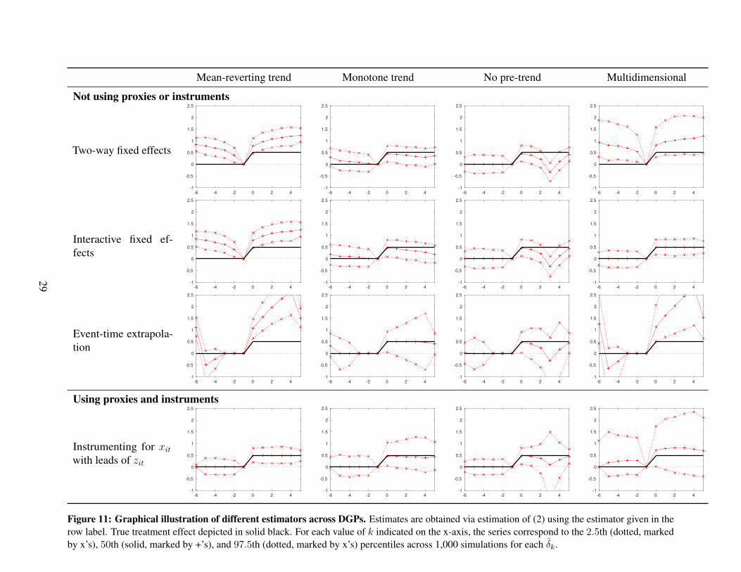
We next examine the performance of feasible estimators for the dynamic treatment effect of thepolicy zit on the outcome yit based on the approaches to identification outlined in Section 3 in eachof the four DGPs. We summarize results in Figure 11. The plots are defined similarly to those inFigure 10 with the lines in the plot corresponding to the median, 2.5th and 97.5th percentile of δkacross 1,000 realizations. These estimates of the event-time path are based on (2) with M +LM = 5
and G + LG = 5. Each column corresponds to a different DGP. Each row now corresponds to adifferent estimator. The black line in each figure gives the true values of the treatment effect forease of reference.
The first row of Figure 11 corresponds to the two-way fixed effects estimator motivated byAssumption 1(a). Across all DGPs the estimated effect of the policy is severely median-biased, withdynamics heavily influenced by the confound.
The second row of Figure 11 corresponds to an interactive fixed effects estimator motivated byAssumption 1(c). We set the number of factors that interact with fixed effects equal to the number ofsources of confounding: one for the “Mean-reverting trend,” “Monotone trend,” and “No pre-trend”DGPs, and two for the “Multidimensional” DGP. Since the DGPs in the first three columns includeconfounding variation that is not captured by a model with shared factors, we see in these threescenarios that interactive fixed effects performs similarly to the baseline two-way fixed effectsestimator. However, the interactive fixed effects estimator performs very well in the final DGPwhere confounding is generated by two shared factors. In this case, the interactive fixed effectsestimator is essentially median-unbiased and overall appears to perform similarly to the infeasibleregression that makes use of the unconfounded outcome.
The third row of Figure 11 corresponds to an estimator motivated by Assumption 2, takingf(m) = 1|m|≤3 following Dobkin et al. (2018). This estimator exhibits substantial median biasin all DGPs except for “Monotone trend,” where the estimator is approximately median-unbiasedbut exhibits substantial variability. Given that it is based on extrapolating pre-event dynamics intothe post-event period, it seems unsurprising that this estimator exhibits median bias in DGPs inwhich the confound’s post-event path is not well-approximated by linear extrapolation of its fittedpre-event path. Because the post-event path of the confound cannot generally be learned from thedata, this finding highlights the importance of motivating assumptions such as Assumption 2 oneconomic grounds.
The final row of Figure 11 corresponds to an instrumental variables (IV) estimator motivatedby Assumption 3(b), following Freyaldenhoven et al. (2019). To obtain the estimates in this case,we make use of the proxy depicted in Figure 10 to stand in for the unobserved confound and theninstrument for this proxy using a lead of the (change in) policy variable. Under the assumption of noanticipatory effects, all leads of the policy variable are potential instruments. For instrument choice,
27

we estimate (2) via two-way fixed effects, with the proxy as the outcome variable. We then choose,from among the leads {∆zi,t+k}G+LG
k=G+1 and zi,t+G+LG, the one with the largest absolute t-statistic
to serve as the excluded instrument for estimation of the structural equation. Graphically, thiscorresponds to imposing the additional restriction that the coefficient on this selected lead is equalto zero. Using only a single lead is appealing because it permits free estimation of the remainingpre-event coefficients and thus visual inspection of the overidentifying restriction that the remainingpre-event effects are zero.9
Having strong identification based on Assumption 3(b) requires that there is a strong associationbetween leads and the proxy variable. We can see in the final row of Figure 10 that only the “Mean-reverting trend” DGP exhibits a strong pre-trend in the proxy. For this DGP, the final row of Figure11 shows that the IV estimator appears to perform well, delivering essentially median-unbiasedresults with sampling variability that is similar to the infeasible regression using the unconfoundedoutcome. A smaller pre-trend in the proxy in the “Monotone trend” DGP means identificationis weaker in this DGP. While the median bias remains relatively low, the weaker identificationresults in a wider sampling distribution. The leads of the policy variable are roughly unrelated tothe policy variable in the “No pre-trend” DGP, leading to a loss of identification and a very widesampling distribution. The IV estimator also performs poorly in the “Multidimensional confound”DGP. As noted above, the proxy is only related to one of the two sources of confounding, leavingan unaccounted-for source of confounding resulting in substantial median bias. The leads are alsorelatively weak instruments in this design which results in a widely dispersed sampling distribution.
Figure 11 shows that, across the estimators and DGPs that we consider, no estimator performsuniformly well. The two-way fixed effects estimator exhibits substantial median bias in all DGPs weconsider. Each other estimator exhibits low median bias for at least one DGP and substantial medianbias for at least one other DGP. No estimator exhibits low median bias for the “No pre-trends” DGP.Because a researcher will not know the true confound or policy effect, it will not in general bepossible to choose estimators based solely on the data, further reinforcing the value of justifyingidentifying assumptions on economic grounds, and of performing sensitivity analysis in situationswhere multiple identifying assumptions are plausible.
9Note that two zero restrictions — that δ−1 and the coefficient on the strongest lead from the first stage are zero —are imposed in each simulation replication. The strongest lead varies across simulation replications due to samplingvariation, so the second restriction is not visually transparent in Figure 11.
28
Mean-reverting trend Monotone trend No pre-trend Multidimensional
Not using proxies or instruments
Two-way fixed effects
-6 -4 -2 0 2 4
-1
-0.5
0
0.5
1
1.5
2
2.5
-6 -4 -2 0 2 4
-1
-0.5
0
0.5
1
1.5
2
2.5
-6 -4 -2 0 2 4
-1
-0.5
0
0.5
1
1.5
2
2.5
-6 -4 -2 0 2 4
-1
-0.5
0
0.5
1
1.5
2
2.5
Interactive fixed ef-fects
-6 -4 -2 0 2 4
-1
-0.5
0
0.5
1
1.5
2
2.5
-6 -4 -2 0 2 4
-1
-0.5
0
0.5
1
1.5
2
2.5
-6 -4 -2 0 2 4
-1
-0.5
0
0.5
1
1.5
2
2.5
-6 -4 -2 0 2 4
-1
-0.5
0
0.5
1
1.5
2
2.5
Event-time extrapola-tion
-6 -4 -2 0 2 4
-1
-0.5
0
0.5
1
1.5
2
2.5
-6 -4 -2 0 2 4
-1
-0.5
0
0.5
1
1.5
2
2.5
-6 -4 -2 0 2 4
-1
-0.5
0
0.5
1
1.5
2
2.5
-6 -4 -2 0 2 4
-1
-0.5
0
0.5
1
1.5
2
2.5
Using proxies and instruments
Instrumenting for xitwith leads of zit
-6 -4 -2 0 2 4
-1
-0.5
0
0.5
1
1.5
2
2.5
-6 -4 -2 0 2 4
-1
-0.5
0
0.5
1
1.5
2
2.5
-6 -4 -2 0 2 4
-1
-0.5
0
0.5
1
1.5
2
2.5
-6 -4 -2 0 2 4
-1
-0.5
0
0.5
1
1.5
2
2.5
Figure 11: Graphical illustration of different estimators across DGPs. Estimates are obtained via estimation of (2) using the estimator given in therow label. True treatment effect depicted in solid black. For each value of k indicated on the x-axis, the series correspond to the 2.5th (dotted, markedby x’s), 50th (solid, marked by +’s), and 97.5th (dotted, marked by x’s) percentiles across 1,000 simulations for each δk.
29

In the Appendix, we extend our analysis to include five additional estimators. Specifically,Appendix Figure A1 considers an estimator that includes the proxy xit directly in the controlsqit, and an estimator motivated by Assumption 1(b), with f(t) = t and so including unit-specificlinear time trends as a control. Appendix Figure A2 considers two versions of a synthetic controlestimator motivated by Assumption 1(c). Finally, Appendix Figure A3 considers a measurement-error correction, assuming the availability of two proxies for the confound, motivated by Assumption3(a). As with the estimators we focus on in the main text, none of these additional estimatorsperforms uniformly well across all DGPs.
4.3 Heterogeneity-Robust Estimation and Heterogeneous Policy Effects
Up to this point we have considered estimators that estimate a single path of policy effects for allunits i. Correspondingly, we have considered DGPs in which the effect of the policy is homogeneousacross units i. In this subsection we consider the consequences of using estimators designed tobe robust to heterogeneity in policy effects. We also consider the consequence for these and otherestimators of drawing data from DGPs that feature such heterogeneity. We do so in three steps.
First, we consider some existing estimators from the literature that are designed to be robustto heterogeneity in policy effects, and apply those to data drawn from our baseline DGPs. Manyrecent papers have proposed approaches to estimating proper weighted averages of policy effectswhen policy effects differ across units or over time. Many of these estimators are grounded inmodels that rule out the forms of confounding exhibited by our DGPs. We might therefore expectthese estimators to perform poorly when applied to data drawn from our DGPs, which featurehomogeneous policy effects but substantial confounding.
Figure 12 illustrates the performance of the estimators proposed by de Chaisemartin andD’Haultfoeuille (2021), Sun and Abraham (2021), and Borusyak et al. (2021a) in data drawn fromour DGPs. These estimators perform similarly to the two-way fixed effects estimator in terms oftheir median bias in these DGPs. Because there is substantial confounding present in these DGPs,the median bias of the estimators is often large. In many cases, the dispersion in the estimator isalso similar to that of the two-way fixed effects estimator, suggesting little statistical cost or benefitfrom adopting the heterogeneity-robust estimator in place of the two-way fixed effects estimator inthese DGPs.
Second, we apply some of the estimators discussed in Section 3 to data drawn from augmentedversions of our baseline DGPs that feature heterogeneity in policy effects across units i. Understaggered adoption, a two-way fixed effects estimator of βm in (1) can be represented as a weightedaverage of policy effects for different event times and cohorts (Sun and Abraham 2021). However,this estimator can put nonzero weight on effects at event times other than m, and can put negativeweight on the effect at event time m for some cohorts. As a result, an estimator of βm based on
30

(1) need not estimate a proper weighted average of cohort-specific policy effects βm,t∗(i) in (13).Appendix Figure A4 depicts the weights across event times and cohorts for the “Mean-revertingtrend” DGP. We indeed find that a two-way fixed effects estimator of βm in (1) is not a properlyweighted average of cohort-specific policy effects βm,t∗(i) in (13) in this design, suggesting thatestimators based on models assuming homogeneous policy effects might perform poorly if thepolicy effects are heterogeneous.
Figure 13 directly illustrates the performance of some of the estimators discussed in Section 3when the policy effect varies by cohort as in (13). Here, we extend the “Mean-reverting trend” DGPto allow for up to two possible dynamic profiles of policy effects. Each unit is assigned to one ofthe two profiles, with the assignment probability dependent on the unit’s cohort t∗(i).10 Figure 13illustrates the four resulting designs with the profiles of policy effects depicted in black.
The first column (“Static, homogeneous policy effect”) corresponds to the “Mean-revertingtrend” DGP, with a homogeneous, static effect of the policy on the outcome. The second column(“Static, heterogeneous policy effect”) allows for two possible static policy effects, one positiveand one null. The third column (“Dynamic, homogeneous policy effect”) features a design with ahomogeneous, dynamic policy effect that builds over time following adoption. The fourth column(“Dynamic, heterogeneous policy effect”) features a design with two possible policy effects, onedynamic (building over time) and one static (no effect).
The first row of Figure 13 considers the infeasible two-way fixed effects estimator applied tothe unconfounded outcome yit − Cit. Under homogeneous policy effects we expect this estimatorto be approximately median-unbiased, and this is what we find. However, as discussed above,this estimator may fail to recover a proper weighted average of the true policy effects underheterogeneous policy effects. This possibility manifests in a spurious pre-trend in the median seriesfor both designs with heterogeneous policy effects.
The second row of Figure 13 considers the feasible two-way fixed effects estimator applied tothe outcome yit. The behavior of this estimator is dominated by the role of the confound. The thirdrow of Figure 13 considers the estimator that instruments for the proxy xit with the strongest leadof the policy zit. This estimator accounts for confounding but not for heterogeneous policy effects.Accordingly, this estimator is approximately median-unbiased in the designs with homogeneouspolicy effects, but exhibits a spurious pre-trend in its median series in the designs with heterogeneouspolicy effects.
10In particular, unit i’s probability of being assigned to the larger of the two policy effects is given by logistic(400−30t∗(i)), so that earlier-adopting cohorts are more likely to be assigned to the larger policy effect. In tandem with ourother design choices, this choice of assignment probability means that almost every unit in the first cohort experiencesthe larger policy effect, almost every unit in the last cohort experiences the smaller policy effect, and similar numbersof units experience each of the two profiles.
31

Mean-reverting trend Monotone trend No pre-trend Multidimensional confound
Baseline estimator
Two-way fixed effects
-6 -4 -2 0 2 4
-1
-0.5
0
0.5
1
1.5
2
2.5
-6 -4 -2 0 2 4
-1
-0.5
0
0.5
1
1.5
2
2.5
-6 -4 -2 0 2 4
-1
-0.5
0
0.5
1
1.5
2
2.5
-6 -4 -2 0 2 4
-1
-0.5
0
0.5
1
1.5
2
2.5
Robust to heterogeneous policy effects
de Chaisemartinand D’Haultfœuille(2020)
-6 -4 -2 0 2 4
-1
-0.5
0
0.5
1
1.5
2
2.5
-6 -4 -2 0 2 4
-1
-0.5
0
0.5
1
1.5
2
2.5
-6 -4 -2 0 2 4
-1
-0.5
0
0.5
1
1.5
2
2.5
-6 -4 -2 0 2 4
-1
-0.5
0
0.5
1
1.5
2
2.5
Sun and Abraham(2021)
-6 -4 -2 0 2 4
-1
-0.5
0
0.5
1
1.5
2
2.5
-6 -4 -2 0 2 4
-1
-0.5
0
0.5
1
1.5
2
2.5
-6 -4 -2 0 2 4
-1
-0.5
0
0.5
1
1.5
2
2.5
-6 -4 -2 0 2 4
-1
-0.5
0
0.5
1
1.5
2
2.5
Borusyak et al. (2021)
-6 -4 -2 0 2 4
-1
-0.5
0
0.5
1
1.5
2
2.5
-6 -4 -2 0 2 4
-1
-0.5
0
0.5
1
1.5
2
2.5
-6 -4 -2 0 2 4
-1
-0.5
0
0.5
1
1.5
2
2.5
-6 -4 -2 0 2 4
-1
-0.5
0
0.5
1
1.5
2
2.5
Figure 12: Estimators designed to allow for heterogeneous effects of the policy. The true treatment effect is depicted in solid black. For each valueof k indicated on the x-axis, the series correspond to the 2.5th (dotted, marked by x’s), 50th (solid, marked by +’s), and 97.5th (dotted, marked by x’s)percentiles across 1,000 simulations for each δk. The first row (“Two-way fixed effects”) implements a two-way fixed effects estimator. The secondrow (“de Chaisemartin and D’Haultfœuille (2020)”) uses the did multiplegt package (de Chaisemartin et al. 2019). The third row (“Sun andAbraham (2021)”) uses the interaction-weighted estimator described in Sun and Abraham 2021 Section 4.1. The fourth row (“Borusyak et al. (2021)”)uses the did imputation package (Borusyak et al. 2021b).
32

Our third and final step in this subsection is to extend the estimators in the second and thirdrows of Figure 13 to allow for different profiles of policy effects by cohort as in (13). We do thisby interacting the policy variables in (2) with indicators for cohort, i.e. for the period in which thegiven unit adopts the policy. We then apply the resulting estimators to the same set of DGPs as inFigure 13, treating the average estimated policy profile across cohorts as our point estimate.
Figure 14 summarizes our findings. Consistent with Sun and Abraham (2021), the modificationto allow for cohort-specific profiles of policy effects ensures that the infeasible estimator recovers aproper weighted average of the possible true profiles of policy effects. This improved performanceextends to the interacted instrumental variables estimator, which no longer exhibits a spuriouspre-trend. The interacted two-way fixed effects estimator performs poorly because of the role ofconfounding. In this setting, then, we find the best performance in terms of bias from an estimatorthat accounts both for heterogeneity in policy effects and for confounding.
Our findings in this section highlight that addressing the possibility of confounding and address-ing the possibility of heterogeneous policy effects are not substitutes for one another. In settingswith severe confounding, estimators designed to recover proper weighted averages of heterogeneouseffects under no-confounding assumptions can perform poorly. Likewise, in settings with limitedor no confounding but significant heterogeneity in policy effects, estimators motivated by modelswith homogeneous policy effects may exhibit undesirable behavior such as spurious pre-trends.Developing additional estimators robust to both confounding and heterogeneous policy effectsseems like a useful direction for future research.
33

Static, homogeneous policyeffect
Static, heterogeneouspolicy effect
Dynamic, homogeneouspolicy effect
Dynamic, heterogeneouspolicy effect
Pooled estimators
Two-way fixed effectsyit − Cit
-6 -4 -2 0 2 4
-1
-0.5
0
0.5
1
1.5
2
2.5
-6 -4 -2 0 2 4
-1
-0.5
0
0.5
1
1.5
2
2.5
-6 -4 -2 0 2 4
-1
-0.5
0
0.5
1
1.5
2
2.5
-6 -4 -2 0 2 4
-1
-0.5
0
0.5
1
1.5
2
2.5
Two-way fixed effectsyit
-6 -4 -2 0 2 4
-1
-0.5
0
0.5
1
1.5
2
2.5
-6 -4 -2 0 2 4
-1
-0.5
0
0.5
1
1.5
2
2.5
-6 -4 -2 0 2 4
-1
-0.5
0
0.5
1
1.5
2
2.5
-6 -4 -2 0 2 4
-1
-0.5
0
0.5
1
1.5
2
2.5
Instrumenting for xitwith leads of zit
-6 -4 -2 0 2 4
-1
-0.5
0
0.5
1
1.5
2
2.5
-6 -4 -2 0 2 4
-1
-0.5
0
0.5
1
1.5
2
2.5
-6 -4 -2 0 2 4
-1
-0.5
0
0.5
1
1.5
2
2.5
-6 -4 -2 0 2 4
-1
-0.5
0
0.5
1
1.5
2
2.5
Figure 13: Graphical illustration of pooled estimators in DGPs with heterogeneous policy effects. All designs are based on the “Mean-revertingtrend” DGP but allow for up to two profiles of possible policy effects, depicted in solid black. Unit i’s probability of being assigned to the largerof the two policy effects is given by logistic(400− 30t∗(i)) where t∗(i) is the period in which unit i adopts the policy. Estimates are obtained viaestimation of (2) using the estimator given in the row label. For the first row, the outcome variable is yit − Cit. For each value of k indicated on thex-axis, the series correspond to the 2.5th (dotted, marked by x’s), 50th (solid, marked by +’s), and 97.5th (dotted, marked by x’s) percentiles across1000 simulations for each δk.
34

Static, homogenous policyeffect
Static, heterogenous policyeffect
Dynamic, homogenouspolicy effect
Dynamic, heterogenouspolicy effect
Interacted estimators
Two-way fixed effectsyit − Cit
-6 -4 -2 0 2 4
-1
-0.5
0
0.5
1
1.5
2
2.5
-6 -4 -2 0 2 4
-1
-0.5
0
0.5
1
1.5
2
2.5
-6 -4 -2 0 2 4
-1
-0.5
0
0.5
1
1.5
2
2.5
-6 -4 -2 0 2 4
-1
-0.5
0
0.5
1
1.5
2
2.5
Two-way fixed effectsyit
-6 -4 -2 0 2 4
-1
-0.5
0
0.5
1
1.5
2
2.5
-6 -4 -2 0 2 4
-1
-0.5
0
0.5
1
1.5
2
2.5
-6 -4 -2 0 2 4
-1
-0.5
0
0.5
1
1.5
2
2.5
-6 -4 -2 0 2 4
-1
-0.5
0
0.5
1
1.5
2
2.5
Instrumenting for xitwith leads of zit
-6 -4 -2 0 2 4
-1
-0.5
0
0.5
1
1.5
2
2.5
-6 -4 -2 0 2 4
-1
-0.5
0
0.5
1
1.5
2
2.5
-6 -4 -2 0 2 4
-1
-0.5
0
0.5
1
1.5
2
2.5
-6 -4 -2 0 2 4
-1
-0.5
0
0.5
1
1.5
2
2.5
Figure 14: Graphical illustration of interacted estimators in DGPs with heterogeneous policy effects. All designs are based on the “Mean-revertingtrend” DGP but allow for up to two possible profiles of policy effects, depicted in solid black. Unit i’s probability of being assigned to the larger of thetwo policy effects is given by logistic(400− 30t∗(i)) where t∗(i) is the period in which unit i adopts the policy. Estimates are obtained via estimationof (13) using the estimator given in the row label. For the first row, the outcome variable is yit − Cit. For each value of k indicated on the x-axis,the series correspond to the 2.5th (dotted, marked by x’s), 50th (solid, marked by +’s), and 97.5th (dotted, marked by x’s) percentiles across 1000simulations for each δk.
35

5 Conclusion
Many important economic applications have been studied using a linear panel model and anaccompanying event-study plot. We have tried to make three contributions in this chapter. The firstis to suggest improvements to the event-study plot, both by codifying what we consider existing bestpractices and also by recommending some practices that are less frequently used. The second is todiscuss some available approaches to identification in the presence of confounds, emphasizing andcontrasting the economic content of the different identifying assumptions. The third is to examinethe performance of estimators corresponding to these approaches to identification under differentpossible economically motivated data-generating processes.
We find that no estimator performs well uniformly under all reasonable DGPs, and that the per-formance of an estimator cannot typically be gauged from the data at hand. These findings highlightthe importance of motivating modeling assumptions on economic grounds, and of developing newstatistical tools grounded in economically motivated assumptions.
36

References
Alberto Abadie, Alexis Diamond, and Jens Hainmueller. Synthetic control methods for comparativecase studies: Estimating the effect of California’s tobacco control program. Journal of the
American Statistical Association, 105(490):493–505, 2010.
Alberto Abadie, Alexis Diamond, and Jens Hainmueller. SYNTH: Stata module to implementsynthetic control methods for comparative case studies, 2020. URL https://ideas.repe
c.org/c/boc/bocode/s457334.html.
Philippe Aghion, Celine Antonin, Simon P. Bunel, and Xavier Jaravel. What are the labor andproduct market effects of automation? New evidence from France. Presentation to the NationalBureau of Economic Research (NBER) Summer Institute Labor Studies, 2020.
Dennis J. Aigner, Cheng Hsiao, Arie Kapteyn, and Tom Wansbeek. Latent variable models ineconometrics. In Zvi Griliches and Michael D. Intriligator, editors, Handbook of Econometrics,volume 2, chapter 23, pages 1321–1393. Elsevier, 1984.
Orley Ashenfelter. Estimating the effect of training programs on earnings. Review of Economics
and Statistics, 60(1):47–57, 1978.
Susan Athey and Guido W. Imbens. Identification and inference in nonlinear difference-in-differences models. Econometrica, 74(2):431–497, 2006.
Susan Athey and Guido W. Imbens. Design-based analysis in difference-in-differences settingswith staggered adoption. Journal of Econometrics, forthcoming.
Susan Athey, Mohsen Bayati, Nikolay Doudchenko, Guido W. Imbens, and Khashayar Khosravi.Matrix completion methods for causal panel data models. Journal of the American Statistical
Association, pages 1–15, 2021. doi: 10.1080/01621459.2021.1891924.
Shalise Ayromloo, Benjamin Feigenberg, and Darren Lubotsky. Employment eligibility verificationrequirements and local labor market outcomes. Presentation to the National Bureau of EconomicResearch (NBER) Summer Institute Labor Studies, 2020.
Jushan Bai. Panel data models with interactive fixed effects. Econometrica, 77(4):1229–1279, 2009.
Emek Basker. Selling a cheaper mousetrap: Wal-Mart’s effect on retail prices. Journal of Urban
Economics, 58(2):203–229, 2005.
Eli Ben-Michael, Avi Feller, and Jesse Rothstein. AUGSYNTH: Augmented synthetic controlmethod, 2020. URL https://github.com/ebenmichael/augsynth.
37

Eli Ben-Michael, Avi Feller, and Jesse Rothstein. Synthetic controls and weighted event studieswith staggered adoption. arXiv:1912.03290, 2021.
Timothy Besley and Anne Case. Unnatural experiments? Estimating the incidence of endogenouspolicies. Economic Journal, 110(467):672–694, 2000.
Stephane Bonhomme and Elena Manresa. Grouped patterns of heterogeneity in panel data. Econo-
metrica, 83(3):1147–1184, 2015.
Kirill Borusyak, Xavier Jaravel, and Jann Spiess. Revisiting event study designs. Working paper,2021a. URL https://6cd96a90-e111-4c99-bb2c-0fdc17ec7c2d.filesusr.
com/ugd/bacd2d c1d299c975204d57b2067545d51630e2.pdf.
Kirill Borusyak, Xavier Jaravel, and Jann Spiess. DID IMPUTATION: Stata module to performtreatment effect estimation and pre-trend testing in event studies, 2021b. URL https://idea
s.repec.org/c/boc/bocode/s458957.html.
Charles Brown. Minimum wages, employment, and the distribution of income. In Orley C.Ashenfelter and David Card, editors, Handbook of Labor Economics, volume 3, chapter 32, pages2101–2163. Elsevier, 1999.
Brantly Callaway and Pedro H. C. Sant’Anna. Difference-in-differences with multiple time periods.Journal of Econometrics, 225(2):200–230, 2021.
Matias D. Cattaneo, Luke Keele, Rocıo Titiunik, and Gonzalo Vazquez-Bare. Extrapolatingtreatment effects in multi-cutoff regression discontinuity designs. Journal of the American
Statistical Association, 2020. doi: 10.1080/01621459.2020.1751646.
Victor Chernozhukov, Christian Hansen, Yuan Liao, and Yinchu Zhu. Inference for heterogeneouseffects using low-rank estimation of factor slopes. arXiv:1812.08089, 2019.
Victor Chernozhukov, Kaspar Wuthrich, and Yinchu Zhu. An exact and robust conformal inferencemethod for counterfactual and synthetic controls. arXiv:1712.09089, 2020.
Clement de Chaisemartin and Xavier D’Haultfoeuille. Two-way fixed effects estimators withheterogeneous treatment effects. American Economic Review, 110(9):2964–2996, 2020.
Clement de Chaisemartin and Xavier D’Haultfoeuille. Difference-in-differences estimators ofintertemporal treatment effects. arXiv:2007.04267, 2021.
38

Clement de Chaisemartin, Xavier D’Haultfoeuille, and Yannick Guyonvarch. DID MULTIPLEGT:Stata module to estimate sharp Difference-in-Difference designs with multiple groups and periods,2019. URL https://ideas.repec.org/c/boc/bocode/s458643.html.
Ellora Derenoncourt, Clemens Noelke, and David Weil. Spillover effects from voluntary employerminimum wages. Presentation to the National Bureau of Economic Research (NBER) SummerInstitute Labor Studies, 2020.
Carlos Dobkin, Amy Finkelstein, Raymond Kluender, and Matthew J. Notowidigdo. The economicconsequences of hospital admissions. American Economic Review, 108(2):308–352, 2018.
Guohua Feng, Jiti Gao, Bin Peng, and Xiaohui Zhang. A varying-coefficient panel data model withfixed effects: Theory and an application to US commercial banks. Journal of Econometrics, 196(1):68–82, 2017.
Simon Freyaldenhoven, Christian Hansen, and Jesse M. Shapiro. Pre-event trends in the panelevent-study design. American Economic Review, 109(9):3307–3338, 2019.
Joachim Freyberger and Yoshiyasu Rai. Uniform confidence bands: Characterization and optimality.Journal of Econometrics, 204(1):119–130, 2018.
Leora Friedberg. Did unilateral divorce raise divorce rates? Evidence from panel data. American
Economic Review, 88(3):608–627, 1998.
Matthew Gentzkow, Jesse M. Shapiro, and Michael Sinkinson. The effect of newspaper entry andexit on electoral politics. American Economic Review, 101(7):2980–3018, 2011.
Andrew Goodman-Bacon. Difference-in-differences with variation in treatment timing. Journal of
Econometrics, 225(2):254–277, 2021.
Zvi Griliches and Jerry A. Hausman. Errors in variables in panel data. Journal of Econometrics, 31(1):93–118, 1986.
Justine S. Hastings, Ryan Kessler, and Jesse M. Shapiro. The effect of SNAP on the composition ofpurchased foods: Evidence and implications. American Economic Journal: Economic Policy, 13(3), 2021.
Catherine Hausman and David S. Rapson. Regression discontinuity in time: Considerations forempirical applications. Annual Review of Resource Economics, 10(1):533–552, 2018.
James Heckman and Jose Scheinkman. The importance of bundling in a Gorman-Lancaster modelof earnings. Review of Economic Studies, 54(2):243–255, 1987.
39

Louis S. Jacobson, Robert J. LaLonde, and Daniel G. Sullivan. Earnings losses of displaced workers.American Economic Review, 83(4):685–709, 1993.
David Neumark and William L. Wascher. Employment effects of minimum and submininum wages:Panel data on state minimum wage laws. Industrial and Labor Relations Review, 46(1):55–81,1992.
David Neumark and William L. Wascher. Minimum wages and employment. Foundations and
Trends in Microeconomics, 3(1–2):1–182, 2007.
Jose Luis Montiel Olea and Mikkel Plagborg-Møller. Simultaneous confidence bands: Theory,implementation, and an application to SVARs. Journal of Applied Econometrics, 34(1), 2019.
M. Hashem Pesaran. Estimation and inference in large heterogeneous panels with a multifactorerror structure. Econometrica, 74(4):967–1012, 2006.
David Powell. Synthetic control estimation beyond comparative case studies: Does the minimumwage reduce employment? Journal of Business & Economic Statistics, 2021. doi: 10.1080/07350015.2021.1927743.
Ashesh Rambachan and Jonathan Roth. An honest approach to parallel trends. Working paper,2021. URL https://jonathandroth.github.io/assets/files/HonestPar
allelTrends Main.pdf.
Jonathan Roth. Pre-test with caution: Event-study estimates after testing for parallel trends. Workingpaper, 2021. URL https://jonathandroth.github.io/assets/files/roth p
retrends testing.pdf.
Jonathan Roth and Pedro H. C. Sant’Anna. When is parallel trends sensitive to functional form?arXiv:2010.04814, 2021.
Kurt Schmidheiny and Sebastian Siegloch. On event study designs and distributed-lag models:Equivalence, generalization and practical implications. CEPR Discussion Paper 13477, 2020.
Azeem Shaikh and Panos Toulis. Randomization tests in observational studies with staggeredadoption of treatment. Working paper, 2021. URL https://cowles.yale.edu/3a/fis
herstaggered-randomization-tests-observational-studies-stagger
ed-adoption-treatment.pdf.
Liangjun Su and Xia Wang. On time-varying factor models: Estimation and testing. Journal of
Econometrics, 198(1):84–101, 2017.
40

Liangjun Su, Zhentao Shi, and Peter C.B. Phillips. Identifying latent structures in panel data.Econometrica, 84(6):2215–2264, 2016.
Liyang Sun. EVENTSTUDYWEIGHTS: Stata module to estimate the implied weights on thecohort-specific average treatment effects on the treated (CATTs) (event study specifications),2021. URL https://ideas.repec.org/c/boc/bocode/s458833.html.
Liyang Sun and Sarah Abraham. Estimating dynamic treatment effects in event studies withheterogeneous treatment effects. Journal of Econometrics, 225(2):175–199, 2021.
Wuyi Wang, Peter C.B. Phillips, and Liangjun Su. The heterogeneous effects of the minimum wageon employment across states. Economics Letters, 174:179–185, 2019.
41

Appendix
Mean-revertingtrend Monotone trend No pre-trend Multidimensional confound
Observed
Outcome yit = 0.5(√
0.5αi +√0.5γt
)+ 0.5zit +
√0.5Cit + 0.5εit
Policy zi1 = 0; ∆zit = 1({
zi,t−1 = 0 and Ci,t+P + 0.5ζzi,t+P < −2})
for t ≥ 2
P = −1 P = 6 P = 3 P = −1
Unobserved
Fixed effects γt = 0.5γt−1 +√0.75ζγt
Confound Cit
Cit =√
1− σ2η
[√1− σ2
a − σ2dλ
′iFt +
√σ2aai +
√σ2ddt
]+
√σ2ηηit, with
dt = 0.5dt−1 +√0.75ζdt
σ2a = σ2
d = σ2η = 0.5, Ft = 0 σ2
η = 0, σ2a = σ2
d = 0.1, dim(Ft) = 2
ηit = ρηηi,t−1 +√
1− ρ2ηζηit
λji =1√2
(1 + ζλji
),
Fjt = ρFjFj,t−1 +
√1− ρ2Fj
ζFjt
ρη = 0.6 ρη = 0.95 ρη = 0.4 ρF1 = 0.9, ρF2 = 0.4
If available
Proxiesxit = 0.5
(√0.5αx
i +√0.5γx
t
)+
√0.5
[√1− θ
(0.5[ai + dt] +
√0.5ηit
)+
√θλ1iF1t
]+ 0.5uit, with
γxt = 0.5γx
t−1 +√0.75ζγ
x
t ; uit = 0.5ui,t−1 +√0.75ζuit
θ = 0 θ = 1
Appendix Table A1: Detailed description of the data-generating processes underlying the simulations presented in Section 4. We generate datafor the time periods t = −4,−3, . . . , T + 5 to avoid missing observations for leads and lags of the policy and to allow for a policy adoption rule that isconsistent with a forward/backward-looking decision-maker on either end of the sample. All random variables not otherwise defined, including initialconditions for autoregressive processes, are distributed as i.i.d. standard normal. We set zit = zi,t−1 if t+ P > T + 5.
42

Mean-reverting trend Monotone trend No pre-trend Multidimensional confound
Baseline estimator
Two-way fixed effects
-6 -4 -2 0 2 4
-1
-0.5
0
0.5
1
1.5
2
2.5
-6 -4 -2 0 2 4
-1
-0.5
0
0.5
1
1.5
2
2.5
-6 -4 -2 0 2 4
-1
-0.5
0
0.5
1
1.5
2
2.5
-6 -4 -2 0 2 4
-1
-0.5
0
0.5
1
1.5
2
2.5
Not using proxies or instruments
Controlling for xit
-6 -4 -2 0 2 4
-1
-0.5
0
0.5
1
1.5
2
2.5
-6 -4 -2 0 2 4
-1
-0.5
0
0.5
1
1.5
2
2.5
-6 -4 -2 0 2 4
-1
-0.5
0
0.5
1
1.5
2
2.5
-6 -4 -2 0 2 4
-1
-0.5
0
0.5
1
1.5
2
2.5
Unit-specific lineartrend
-6 -4 -2 0 2 4
-1
-0.5
0
0.5
1
1.5
2
2.5
-6 -4 -2 0 2 4
-1
-0.5
0
0.5
1
1.5
2
2.5
-6 -4 -2 0 2 4
-1
-0.5
0
0.5
1
1.5
2
2.5
-6 -4 -2 0 2 4
-1
-0.5
0
0.5
1
1.5
2
2.5
Appendix Figure A1: Additional estimators not using proxies or instruments across DGPs. The true treatment effect is depicted in solid black.For each value of k indicated on the x-axis, the series correspond to the 2.5th (dotted, marked by x’s), 50th (solid, marked by +’s), and 97.5th (dotted,marked by x’s) percentiles across 1000 simulations for each δk. The first row (“Two-way fixed effects”) implements a two-way fixed effects estimator.The second row (“Controlling for xit”) includes the proxy xit directly in the controls qit. The third row (“Unit-specific linear trend”) allows forunit-specific linear time trends.
43

Mean-reverting trend Monotone trend No pre-trend Multidimensional confound
Baseline estimator
Two-way fixed effects
-6 -4 -2 0 2 4
-1
-0.5
0
0.5
1
1.5
2
2.5
-6 -4 -2 0 2 4
-1
-0.5
0
0.5
1
1.5
2
2.5
-6 -4 -2 0 2 4
-1
-0.5
0
0.5
1
1.5
2
2.5
-6 -4 -2 0 2 4
-1
-0.5
0
0.5
1
1.5
2
2.5
Not using proxies or instruments
Synthetic control (sim-plex)
-6 -4 -2 0 2 4
-1
-0.5
0
0.5
1
1.5
2
2.5
-1.5
-1
-0.5
0
0.5
1
1.5
-6 -4 -2 0 2 4
-1
-0.5
0
0.5
1
1.5
2
2.5
-1
-0.5
0
0.5
1
1.5
2
-6 -4 -2 0 2 4
-1
-0.5
0
0.5
1
1.5
2
2.5
-1
-0.5
0
0.5
1
1.5
2
-6 -4 -2 0 2 4
-1
-0.5
0
0.5
1
1.5
2
2.5
-1
-0.5
0
0.5
1
1.5
2
Synthetic control (un-constrained)
-6 -4 -2 0 2 4
-1
-0.5
0
0.5
1
1.5
2
2.5
-1
-0.5
0
0.5
1
1.5
2
-6 -4 -2 0 2 4
-1
-0.5
0
0.5
1
1.5
2
2.5
-1
-0.5
0
0.5
1
1.5
2
-6 -4 -2 0 2 4
-1
-0.5
0
0.5
1
1.5
2
2.5
-1
-0.5
0
0.5
1
1.5
2
-6 -4 -2 0 2 4
-1
-0.5
0
0.5
1
1.5
2
2.5
-1
-0.5
0
0.5
1
1.5
2
Appendix Figure A2: Synthetic control estimators across DGPs. The true treatment effect is depicted in solid black. For each value of k indicatedon the x-axis, the series correspond to the 2.5th (dotted, marked by x’s), 50th (solid, marked by +’s), and 97.5th (dotted, marked by x’s) percentilesacross 1000 simulations for each δk. The right axis depicts the estimated treatment effect relative to the synthetic control. On the left axis, estimates arenormalized such that the median treatment effect is zero the period before the event. The donor pool for unit i in cohort t∗(i) consists of all units jwith t∗(j) > t∗(i) + 5 and all units j that never adopt the policy, and weights are chosen to fit the path of the outcome variable in all periods priorto t∗(i). The first row (“Two-way fixed effects”) implements a two-way fixed effects estimator. The second row (“Synthetic control (Simplex)”)estimates δk using the synth package (Abadie et al. 2020), restricting the weights on the donor units to the simplex. The third row (“Synthetic control(Unconstrained)”) estimates δk using the augsynth package (Ben-Michael et al. 2020), allowing donor weights outside the simplex but imposing anℓ2-penalty of 0.001.
44

Mean-reverting trend Monotone trend No pre-trend Multidimensional confound
Baseline estimator
Two-way fixed effects
-6 -4 -2 0 2 4
-1
-0.5
0
0.5
1
1.5
2
2.5
-6 -4 -2 0 2 4
-1
-0.5
0
0.5
1
1.5
2
2.5
-6 -4 -2 0 2 4
-1
-0.5
0
0.5
1
1.5
2
2.5
-6 -4 -2 0 2 4
-1
-0.5
0
0.5
1
1.5
2
2.5
Using proxies and instruments
Instrumenting for x1itwith second proxy x2it
-6 -4 -2 0 2 4
-1
-0.5
0
0.5
1
1.5
2
2.5
-6 -4 -2 0 2 4
-1
-0.5
0
0.5
1
1.5
2
2.5
-6 -4 -2 0 2 4
-1
-0.5
0
0.5
1
1.5
2
2.5
-6 -4 -2 0 2 4
-1
-0.5
0
0.5
1
1.5
2
2.5
Appendix Figure A3: Additional estimator using proxies and instruments across DGPs. The true treatment effect is depicted in solid black. Foreach value of k indicated on the x-axis, the series correspond to the 2.5th (dotted, marked by x’s), 50th (solid, marked by +’s), and 97.5th (dotted,marked by x’s) percentiles across 1000 simulations for each δk. The first row (“Two-way fixed effects”) implements a two-way fixed effects estimator.The second row (“Instrumenting for x1it with second proxy x2it”) considers a measurement-error correction, assuming the availability of two proxies forthe confound, by instrumenting for one proxy, x1it, with the other, x2it.
45

Furthest lead Event-time coefficient Furthest lag
Weights from a single realization
---
-
-
---
-
-
--
-
-
-
-
-----
---
-
-
--------
---
-
------
-
-
----------
-
---------------------
-----
--------------------------
-------------------------
-----------------
----------------
--------------
-------------
-----------
+++++++++++++++++++++++++++++
++++++
+
+++++++++++++++++++++++++++
+
+++++
++
+++++++++++++++++++++++++++
+
+++++
+++
+++++++++++++++++++++++++++
+
+++++
++++
++++++++++++++++
++
+
+++++
++++++
+++++++++++++
++
++++++
+++++++
+
++
++
+++++
+++++++++++
++
++++++++++++
++++++++++++++
+++++++++++++++
+++++++++++++++++++++++
++++++++++++++++++++++++
++++++++++++++++++++++++++
+++++++++++++++++++++++++++
+++++++++++++++++++++++++++++
5 10 15 20 25 30 35 40
Cohort
40
30
20
10
0
-10
-20
-30
-40
Event tim
e
0
0.02
0.04
0.06
0.08
0.1
0.12
------
--
--
-
-----
-
-
-
-
-
--
------
--
-
-
-
-
--
-
-
-
------
--
-
-
-
-
-
-
-
-
------
-
-
-
-
-
--
--
-
-
-
-
-
-
-
-
--
-
-
-
-
-
-
-
-
-
-
-
-
-
-
-
-
-
-
-
-----
-
-
-
-
-
-
--
-
--
----
-
-
-
-
-
-
-
-
--
-
----
-
-
-
-
-
-
-
---
-
----
-
-
-
-
-
-
-
--
-----
---
-
----
-
-
-
-
-
-
--
------
---
-
----
-
-
-
-
-
---
--------
---
-
----
-
-
-
-
-
--
---------
---
-
----
-
-
---
--
---------
---
-
----
-
-
+
+
+
++
++++
+
+++
++
+
+
+
+
+++++++++
++++
+
+++
+
++
+
+
+
+++++++++
++++
+
+++
++
+
++
+
++
+++++++++
++++
+
++
+++
++
+++++
+
++
+++++++++
++++
+
+++
+
+
++
+++++
+
++
+++++++++
++++
+
++
+
+
+
++
+++++
+
++
+++++++++
++
+
++
+
+
++
+++++
+
++
+++++++++
++
+
+
+
+
++
+++++
+
++
+++++++++
+
+
+
+
+
+
++
+++++
+
++
++++++++++
+
+
+
+
+
++
+++++
+
++
+
+
+
+
+
+
+
+
++
+++++
+
+++
+
+
+
+
+
+
+
++
+++++
+
+
++
+
+
+
+
+
++
+++++
++
+
+
+
+
+
+
+
+++
++++++
+
+
+
+
+
+
+
+++
5 10 15 20 25 30 35 40
Cohort
40
30
20
10
0
-10
-20
-30
-40
Event tim
e
0
0.02
0.04
0.06
0.08
0.1
0.12
--
-
--
---
----
----
-
--
-------
--
-------
-
--
--------
----
-----------------
-----
-----------
----
----
--------
-
--
----
------------
-
--
-
----
---
-
---
-
-----
---
-
---
-
-------
---
-
-
-
--------
---
-
----
+++++++++++++++++++++++++++++++++
+
+
++++++++++++++++++++++++++++++++
+
+++++++++++++++++++++++++++++++
+
+
++++++++++++++++++++++++++++++
+
++++++++++++++++++++++++++++
+
+
+++++++++++++++++++++++++++
+
+++++++++++++++++++++++
+++++++++++++++++++++++
+
+++++++++++++++++
+
+
+
+
++++++++++++++++++
+
+
+
++++++++++++
++++
++
+
+
++++++++
+++++++++++
++++
++
+
+
++++++++
+++++++++
++++
++
+
+
++++++++++
++++++++
++++
++
++++++++++++++
++++++
++++++
+++++++++++++++++++++++
5 10 15 20 25 30 35 40
Cohort
40
30
20
10
0
-10
-20
-30
-40
Event tim
e
0
0.02
0.04
0.06
0.08
0.1
0.12
Weights averaged over 100 realizations
-------
-
------
-
-----
-
----
-
--
-
-
--
--
-
-------
-
--------
-
-----------
-
--------------
-
-
--------------
-
-
---------------
-
-
--
---------------
-
----------------------
-
-----------------------
-
---------------------
--
----------------------
--
------------------
----
-
----------------------
-
------------------------
----------------------
-
---------------------
----------------------
---------------------
-----------------
--
-------------------
------------------
-----------------
----------------
---------------
--------------
-------------
------------
-----------
----------
---------
--------
-------
------
+++++++++++++++++++++++++++
+++++
+++++++++++++++++++++++++++
+++++
+
+++++++++++++++++++++++++++
+++++
++
+++++++++++++++++++++++++++
+++++
+++
++++++++++++++++++++++++++++
+++++
++++
+++++++++++++++++++++
++
+
+++++
+++++
+++++++++++++++++++++
+++++
++++++
+++++++++++++++++++
+++++
+++++++
+++++++++++++++
+++++
++++++++
+++++++++++
+++++
+++++++++
++++++++
+
+++++
++++++++++
++++
+++
+++++
+++++++++++
+
+
++
+++++
++++++++++++
++++
+++++++++++++
++
++++++++++++++
++
+++++++++++++++
+
+++++++++++++++
+
++
++++++++++++++
+
++++++++++++++++
++++++++++++++++
+
++++++++++++++++
+++++++++++++++++++
++++++++++++++++++
+++++++++++++++++++
+
++++++++++++++++++++
+++++++++++++++++++++
++++++++++++++++++++++
+++++++++++++++++++++++
++++++++++++++++++++++++
+++++++++++++++++++++++++
++++++++++++++++++++++++++
+++++++++++++++++++++++++++
++++++++++++++++++++++++++++
+++++++++++++++++++++++++++++
++++++++++++++++++++++++++++++
+++++++++++++++++++++++++++++++
++++++++++++++++++++++++++++++++
+++++++++++++++++++++++++++++++++
++++++++++++++++++++++++++++++++++
5 10 15 20 25 30 35 40
Cohort
40
30
20
10
0
-10
-20
-30
-40
Event tim
e
0
0.02
0.04
0.06
0.08
0.1
0.12--
-
-
-
--
---
----
-
--
-
-
-
--
-
--
----
-
-
--
--
-
-
-
-
--
--
-
-
--
--
--
-
-
-
-
--
-
-
-
-
-
-
--
--
--
--
-
-
-
-
---
-
--
-
-
-
-
-
--
---
-
-
-
-
--
-
-
-
-
-
----
--
---
--
-
-
--
--
-
-
----
--
--
-
--
-
--
---
-
-
--
-
-
--
-
-
--
-
-
--
--
--
--
---
---
---
--
-
--
--
--
---
-
-
-
--
--
--
-
-
-
-
-
-
--
-
---
--
--
--
---
-
-
---
-
-
-
--
-
-
-
-
--
-
-
--
--
-
-
--
--
--
-
----
-
-
--
-
--
-
-
-
-
-
--
---
-
--
---
-
-
-
-
-
--
--
--
-
----
---
-----
-
-
-
-
--
-
-
---
---
-
-
--
--
-
-
---
----
--
--
--
--
-
--
-
-
---
-
------
--
--
-
-
-
-
--
--
--
--
-
--
---
--
-
-
-
-
---
-
-
----
---
---
-
--
-
--
-
-
-
--
-
-
--
-
--
-
--
-
-
-
----
-
-
-
-
-
-----------
--
--
-
-
-
-
----
-
----
---
-
--
--
-
-
-
-
-
--
---
--
---
-
--
-
-
-
-
-
-
--
-----
--
---
---
-
--
-
-
--
--
--
--
---
---
-
-
-
-
-
-
-
-
---
-
-
---
--
--
--
---
--
-
-
-
-
----
-
--
-------
-
-
-
-
-
-
--
-
-
-
----
--
---
--
-
-
-
-
-
-
--
-----
---
--
-
---
-
-
----
--
-
--
-
---
---
-
-
-
-
-
--
-
---
-------
--
-----
-
-
-
---
--
---
----
--
-
-
-
----
--
--
------
-----
-
-
-
--
-
--
--
--
--
-
---
------
-
-
--
-
--
-
-
-
--
-
-
------
-
-
----
-
-
---
-
--
---
-
---
-
-
-
---
-
-
-
--
-
--
---
--
-
---
-
---
-
--
---
-
-
--
--
--
-
--
-
-
---
-
---
---
-
-
---
-
-
---
-
-
--
--
---
----
+
+
+++
++
+
+
++
+
+
+
+
+
+
++
++
++
+
+
+
+
+
++
+
+
+
+
+
+
+
++
++
+
+
+
++
+
++
+
+
++
+
+
+
+
+
+
+++
+
+
+
+++
+
+
+++
+
+
+
++
+
+
+
+
++
+
+
+
+++
+
+
+
+
+
+++
+
++
++
+
++
+
+
+
+
+
+++
++
+
+++
++
+++
++
+
++
+
+
+
++
+
+
+
+
++
+++
+++
+
+
+
+
+
+
+
++
+
+
+
+
+++
++
++
+
+
+
+
++++
++
++
+
+
++
+++
+
+
+
+
+
+
+
+
++
++
+
+
++
++
+
++
+
+
+
+
+
++++
++
++++
++
++
+
+
+
+
+
+
++
++
+
+++
++++
++
+
+
+
+
+
+
++
+
+++
++
+
++++
+++
+
+
+
+
+++
++
++
+
++++
+
+
++
+
+
+++
+
+
+
++
++++
+
+
++
+
+++
++++
++++
+
++++++
+
+
+
+
+
++
+
+++
++
+
++
++
+
+
+
+
+
+
+
+
+
++
+
++++
+++
+++
+
+
+
+
+
+
+
+
++
++
++
++++
+
+
+
+
+
+
+
+
+
++
++
++
+
+
+
+
+
+
+
+
++
++
+++
++++
+
+
+
+
++
+
+
+
+
++
+
+++
+++
++
+
+
+
+
++
+
+
++
++
+
+++
++
+
+
+
+
+
+
+
+
+
+++
+
+++
+++
+
+
+
+
+
+
+
+
+++
+
+
+
++
+
++
+
+
+
+
+
+
++++
+
+
+
+
+
+
+
+
+
+
+
++
++
+
+++++
+
+
+
++
+
+
+
+
++++
++++
+
+++
+
+
+
+
+
+
+
+
++
+++
+++
++
+
++
+
++++
+
+
++
+
+
+
+
++
++
+
+
+
+
+
+++
++
++++
+
+
+
+
+
+
+
+
+++
++
+++
+++
+
+
+
++
+
+
+
+
+++
+
+
+
+
++
+
+
++
+
++
+
+++++
++
++
++
+
++
+
+
+
+
+
+
++
+
++
++
+
+
+
+
++
+
+
+
+
+
+
+
+
+
+
+
+
+
++
+
+
+
+
+
++
+
+
+
+
+
+
++
+
+
++
+
+
+
+
++
+
+
+
++
+
+
++
+
++
+
+
5 10 15 20 25 30 35 40
Cohort
40
30
20
10
0
-10
-20
-30
-40
Event tim
e
0
0.02
0.04
0.06
0.08
0.1
0.12--
------
-------
--------
---------
----------
-----------
------------
-------------
------
------
-------
-
-----
---------
------
-----------------
-----------------
-------------------
--------------------
---------------------
--------
------------
-------------------
--
------------
-
---
-----------
-
-
-
------------
-
-
---
----------
--
-
--
----------
-
-
------------
-
------------
--
------------
-
----------
-
-----------
-
---------
---
-
-------------
-
---------
-
----------
-
----------
-
-----
--
-
------
-
-
--------
-
-
--------
-
---------
-
-------
--
++++++++++++++++++++++++++++++++
+++++++++++++++++++++++++++++++++
++++++++++++++++++++++++++++++++
+++++++++++++++++++++++++++++++
++++++++++++++++++++++++++++++
+++++++++++++++++++++++++++++
++++++++++++++++++++++++++++
+++++++++++++++++++++++++++
++++++++++++++++++++++++++
++
+++++++++++++++++++++++++
+
+
++++++++++++++++++++++++
+
+++++++++++++++++++++++
+++++++++++++++++++++++
+++++++++++++++++++++
++++++++++++++++++++
+++++++++++++++++++
++++++++++++++++++
+
+
+++++++++++++++++++
++
++++++++++++++++++++
+
+++
+
+++++++++++++++++++
+
+
++++
+++++++++++++++++++
+
+
++
++
++++++++++++++++
+
++
+
++++
+++++++++++++++++
+
+
++
+++++
++++++++++++++++
++++
+++++++
+++++++++++++++
++++
++++++++
++++++++++++++
+++
+++++++++
+++++++++++++
++++
++++++++++++
++++++++++++
++++
++++++++++++
+++++++++++
++++
+
+++++++++++
++++++++++
++++
++++++++++++
+++++++++
++++
+++++++++++++++++
++++++++
++++
+++++++++++++++++
+++++++
++++
++++++++++++++++++
++++++
++++
+++
+++++++++++++++++++
+++++
++++
++++
+++++++++++++++++++
++++
++++
++
++++++++++++++++++++
+++
++++
++++++++++++++++++++++++
++
++++
++++++++++++++++++++++++
+
++++
+
++++++++++++++++++++++++
5 10 15 20 25 30 35 40
Cohort
40
30
20
10
0
-10
-20
-30
-40
Event tim
e
0
0.02
0.04
0.06
0.08
0.1
0.12
Appendix Figure A4: Graphical illustration of weights underlying coefficients. The figure shows the estimated weights underlying the coefficientsδ−6 (“Furthest lead”), δ0 (“Event-time coefficient”), and δ5 (“Furthest lag”) from the model in (2) with M + LM = 5 and G+ LG = 5. In each plot,the shading of each cell denotes the absolute estimated weight that corresponds to the given cohort and event time, and the symbol (+ or −) denotesthe sign of the estimated weight. The first row (“Weights from a single realization”) shows the estimated weights from a single realization from the“Mean-reverting trend” DGP. The second row (“Weights averaged over 100 realizations”) shows the average estimated weights across 100 realizationsof the “Mean-reverting trend” DGP. The weights are defined following Proposition 1 of Sun and Abraham (2021) and estimated following equation(13) of Sun and Abraham (2021) using the package eventstudyweights (Sun 2021).
46