ISSN 1060�992X, Optical Memory and Neural Networks (Information Optics), 2012, Vol. 21, No. 4, pp. 227–232. © Allerton Press, Inc., 2012.

227

INTRODUCTION

Ever�growing information about systems and processes and diversity of analyzing methods make thefinding of regularities in multiple�parameter data a very topical issue. Visualization methods can be a veryuseful tool for effective analysis of high�dimensional data.

The visualization of high�dimensional data is understood [1] as a one�dimensional or two�dimensionalrepresentation that can give at least a clear idea of the regularities inherent in the original distribution.

Let a set of data n > 3 be given. Visualization of set Xrequires us to find a representation functional

( or ) (1)

that would minimize a given criterion of quality

(2)

The conventional approach to visualization of high�dimensional data is the use of the principal com�ponent analysis [2] whose idea is to build a linear manifold (map) into which the data are mapped. Themethod effectively solves the problem in the case of a simple unimodal data structure. More complex datastructures required the development of nonlinear methods of visualization such as Sammon maps [3],principal manifolds method [4], self�organizing maps [5], elastic maps [1].

Sammon maps, principal manifolds method and elastic maps suggest a nonlinear structure of maps.Building such maps requires a great number of complex optimization problems to be solved, which makesthese methods ineffective for visualization of large amounts of high�dimensional data. The simple and fastlearning algorithm of Kohonen maps allows us to build piecewise�linear maps which effectively approxi�mate high�dimensional data structures.

Though the approach made it possible to solve the general problem of visualization of high�dimen�sional data of complex topology, it gave rise to other snags. The modifications of the SOM method (e.g.the regularization method [6], Bacth SOM algorithms [7], adaptive SOM [8], hierarchical algorithms [9],neural gas [10]) improve the Kohonen maps algorithm in many ways, yet the problem of mapping ontothe edges or nods of piecewise�flat Kohonen maps is caused by the piecewise�linear structure of maps andcan’t be solved by modification of the learning algorithm of the Kohonen neural network.

1{ ,..., },NX X X= ( )1 ,..., ,Tc c c

nX x x= 1, ,c N=

: n mU R R→ 1m = 2m =

( ), min.Q U X →

Visualization of High�Dimensional Data Using Two�Dimensional Self�Organizing

Piecewise�Smooth Kohonen MapsA. V. Shklovets and N. G. Axak

Kharkov National Radioelectronics University, Ukrainee�mail: ashklovets@mail.ru, axak@kture.kharkov.ua

Received March 19, 2012; in final form, September 10, 2012

Abstract—To make visualization of high�dimensional data more accurate, we offer a method ofapproximating two�dimensional Kohonen maps lying in a multiple�dimensional space. Cubic para�metric spline�based least�defect surfaces can be used as an approximation function to minimizeapproximation errors.

Keywords: visualization of high�dimensional data, two�dimensional piecewise�smooth Kohonenmaps, parametric spline�based surface

DOI: 10.3103/S1060992X12040066

228

OPTICAL MEMORY AND NEURAL NETWORKS (INFORMATION OPTICS) Vol. 21 No. 4 2012

SHKLOVETS, AXAK

SETTING THE PROBLEM

Suppose that after a Kohonen map has been learnt on a data set X in an n�dimensional Euclidean

space, the output neurons have coordinates l is the number of

output neurons. Triangulation is defined on set W, where

M is the number of triangles, is the number of a neuron in set W, For tackling theproblem it is necessary to build a piecewise�smooth SOM by approximating the piecewise�linearKohonen map by a parametric least�defect spline�based surface.

PARAMETRIC SPLINE�BASED SURFACE

Let partition Δ is defined of subdomain Ωk of a particular flat manifold Ω enclosed in space

( NΩ is the number of subdomains of partition Δ). Vector�valued function [11]

(3)

is called a two�dimensional parametric spline surface of dimensionality m1 of defect with parameter t1

and dimensionality m2 of defect ν2 with parameter t2 if for each subdomain Ωk of grid Δ there is vector�valued function

(4)

whose parameters vary within a certain domain Here function is a polynomial ofdegree m1 by parameter t1 and degree m2 by parameter t2

(5)

(6)

Third�order splines are the best solution from the accuracy�complexity viewpoint. Further we will

assume that m1 = m2 = 3, and have the smallest values. Let

and Parameters of spline surface S(t1, t2) form four�dimensional

matrix = holding NA = 16nNΩ parameters in all.

GENERATING A PIECEWISE�SMOOTH SOM

In our consideration manifold Ω is triangulation T divided in M triangles Each triangle isput in correspondence with a certain cubic parametric surface (1) whose parameters are defined over a tri�angle {(0,0); (1,0), (0,1)}.

In paper [12] the authors offer making up a set of linear algebraic equations to define the parameters

of spline surface A. This set defines the relationship between the parameters. Using condition ofpassing at points {(0,0); (1,0), (0,1)} of the topological coordinate system through the corresponding

points of the n�dimensional Euclidean space, we can write 3nM equations:

(7)

1{ ,..., }lW W W= ( )1,..., ,Ti i i

nW w w= 1, ,i l=

{ }1,..., MT T T= { }1 2 3, , ,k k k kT T T T= 1, ,k M=

kpT { }1, ,k

pT N∈ 1,3.p =

,W T

nR

1, ,k NΩ=

( ) ( ) ( )( )1 2 1 2 1 2 1 2 1 2 1 2, , , 1 2 , , , ,1 1 2 , , , , 1 2, , ,.., ,m m m m m m nS t t s t t s t t=

v v v v v v

1v

( ) ( ) ( )( )1 2 1 2 1 2 1 2 1 2 1 2, , , 1 2 , , , ,1 1 2 , , , , 1 2, , ,.., ,k

k k km m m m m m nS t t s t t s t t

Ω

=v v v v v v

�

2.k RΩ ∈� ( )1 2 1 2, , , , 1 2,k

m m ps t tv v

( )1 2

1 2 1 2, , , , 1 2 1 2

0 0

, ,m m

k k i jm m p ijp

i j

s t t a t t= =

=∑∑v v1, ,k NΩ= 1, ,p n=

( ) ( )1 2 1 2 1 2 1 2, , , 1 2 , , , 1 2

1

, , .N

km m m m

k

S t t S t tΩ

Ω

=

=v v v v∪

1v 2v ( ) ( )1 23,3, , 1 2 1 2, , ,k kS t t S t t=

v v

( ) ( )1 23,3, , 1 2 1 2, , ,S t t S t t=

v v ( )1,.., .k k kij ij ijnA a a=

( )1,

0,3; 0,3

k Nkij

i jA A

Ω=

= =

= ( )1,

0,3; 0,3; 1,

k Nkijp

i j p na

Ω=

= = =

.kT T∈kT

( )1 2,kS t t

{ }1 2 3, ,k k kT T TW W W

( )

( )

( )

11

1 2

2 2

1 2

3

1 23

001 2 0, 03

1 2 1, 0 0

0

31 2 0, 1

0

0

,, ,

, , ,

, ,.

kk

k k

k

k

k Tk Tt t

k T k Tt t i

ik T

t tk T

j

j

A WS t t W

S t t W A W

S t t WA W

= =

= =

=

= =

=

⎧⎪

⎧ ⎪ ==⎪ ⎪⎪ ⎪

= ⇒ =⎨ ⎨⎪ ⎪⎪ ⎪=⎩ ⎪ =

⎪⎩

∑

∑

1,k M=

OPTICAL MEMORY AND NEURAL NETWORKS (INFORMATION OPTICS) Vol. 21 No. 4 2012

VISUALIZATION OF HIGH�DIMENSIONAL DATA 229

To form the conditions of smooth joint, let us consider two triangles and Let these tri�

angles share one side, which means that two nodes of the triangles and coincide. Then the smooth�joint condition takes the form:

(8)

where Ω is the curve of contact of two surfaces and The sides of two triangles can contact in 21 ways. Set (8) can give either 12n or 18n linear equations for

each occasion of contact. After analyzing all pairs of triangles for side contacts and making the above�mentioned set of linear algebraic equations, it is necessary to determine its rank r.

If the offer is to delete (r – NA) nonequivalent equations from the set, which results in thedefect of the spline surface getting smaller. This way, the set of equations will become consistent and havea unique solution which defines the parameters of the spline surface.

If , the offer is to use (NA – r) parameters to define r parameters. The other parameters can bedefined by minimization of departure of the spline surface from the piecewise�flat map

(9)

The goal function is the sum of distances from each triangle to the corresponding surface .After disclosure of the second integral, the goal function has the second order and can be solved analyti�cally. The detail consideration of the method is given in article [13].

Among the disadvantages of the method are the necessity to determine the rank of the set of equationsand difficulties in finding the solution to the equations obtained in the case when triangles contact alongthe side {(1,0); (0,1)}.

In order to overcome the difficulties in solving the set of linear algebraic equations, the authors of paper

[14] offer the method of building quadrangular Kohonen maps based on the Delone�triangulation�like maps T. The optimization problem (9) for quadrangular maps looks like

(10)

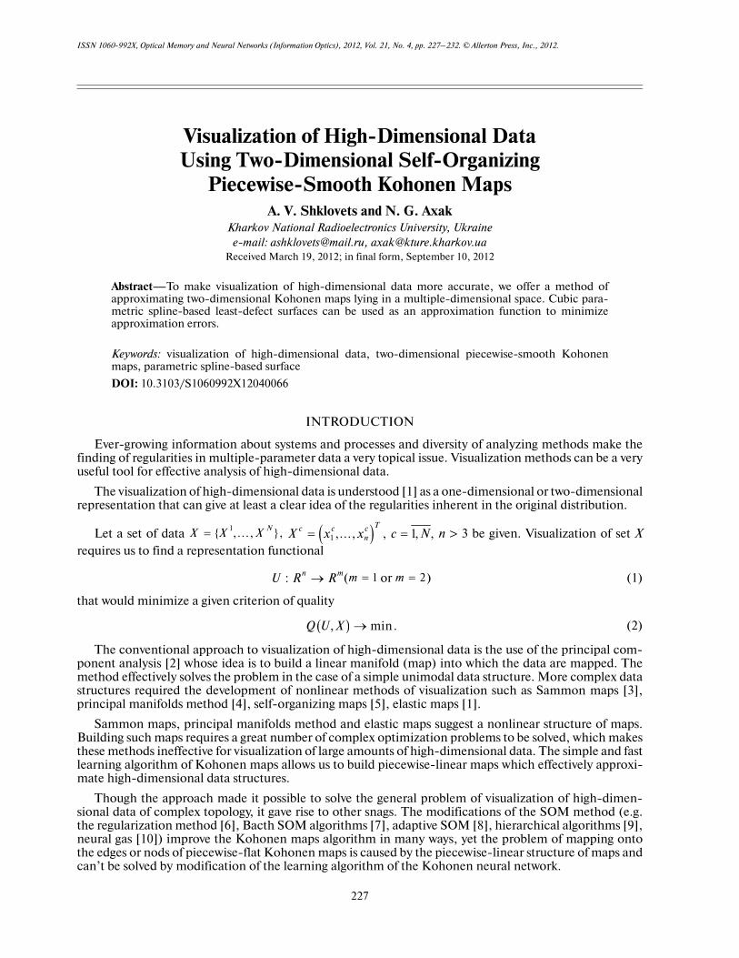
The use of quadrangular maps can speed up generation of piecewise�flat Kohonen maps.Rectangular and hexagonal Kohonen maps of size l1 × l2 = l neurons are particular cases of quadran�

gular Kohonen maps. It is seen from Figure 1 that this kind of maps are isomorphic with regard to spline�surface approximation.

Article [15] gives the analysis of the set of algebraic linear equations for parameters for rectangular andhexagonal Kohonen maps. The set holds equations and its rank is

(11)

If we express the parameters of the spline surface by using

(12)

we can solve the set by the sweep method for time the sweep time changing linearly.

1kT T∈2 .kT T∈

1kT 2kT

( ) ( )( ) ( )

( ) ( )

1 2

1 2

1 2

1 2 1 21 2 1 2

1 1

2 21 2 1 2

2 21 1

, ,, ,

, ,

k kk k

k k

S t t S t tS t t S t t

t t

S t t S t t

t t

∂Ω ∂Ω ∂Ω ∂Ω

∂Ω ∂Ω

∂ ∂= = −

∂ ∂

∂ ∂=

∂ ∂

( )11 2,kS t t ( )2

1 2, .kS t t

,Ar N≥

Ar N<

( ) ( ) ( )( )1

1 3 1 2 1

1 12

1 1 2 1 2 2

1 1 0 0

, min .k k k k k

tM nk T T T T Tp p p p p p

k p

dt s t t x x x t x x t dt

−

= =

− − − − − →∑∑ ∫ ∫kT ( )1 2,kS t t

( )1 /2,..., MQ Q Q=

( ) ( ) ( )( )

( ) ( ) ( )( )

1

1 3 1 2 1

1

4 2 4 3 4

1 12 2

1 1 2 1 2 2

1 1 0 0

1 12

1 1 2 1 2 2

0 0

,

1 ,1 min .

k k k k k

k k k k k

Mtn

k Q Q Q Q Qp p p p p p

k p

t

k Q Q Q Q Qp p p p p p

dt s t t x x x t x x t dt

dt s t t x x x t x x t dt

−

= =

−

⎡⎢ − − − − −⎢⎣

⎤⎥+ − − − − − − − →⎥⎦

∑∑ ∫ ∫

∫ ∫

( ) ( ) ( )1 2 1 228 1 1 12 2n l l n l l− − − − −

( ) ( ) ( ) ( )[ ] ( ) ( ) ( ) ( )[

( ) ( )] ( ) ( ) ( ) ( )+ 1 2 1 2 1 2 1 2

1 2 1 2 1 2

28 1 1 12 1 12 1 2 1 2 2 2 1

8 2 2 16 1 1 2 1 2 1 8 .

r n l l n l n l n l l n l l

n l l n l l n l n l n

= − − − − − − − − − + − −

− − = − − − − − − −

( ) ( ) ( ) ( ){ }1 1 2 2,1 ,1 1, 1,(1,1) (1,1) (1,1) (1,1) (1,1) (1,1) (1,1) (1,1) (1,1) (1,1) (1,1) (1,1)01 02 10 11 12 13 20 21 22 23 31 32 31 32 13 23

1 1 2 2

, , , , , , , , , , , , , , , ,

2, 1, 2, 1

k k k kA A A A A A A A A A A A A A A A

k l k l= − = −

( )( )1 2 ,O n l l+

230

OPTICAL MEMORY AND NEURAL NETWORKS (INFORMATION OPTICS) Vol. 21 No. 4 2012

SHKLOVETS, AXAK

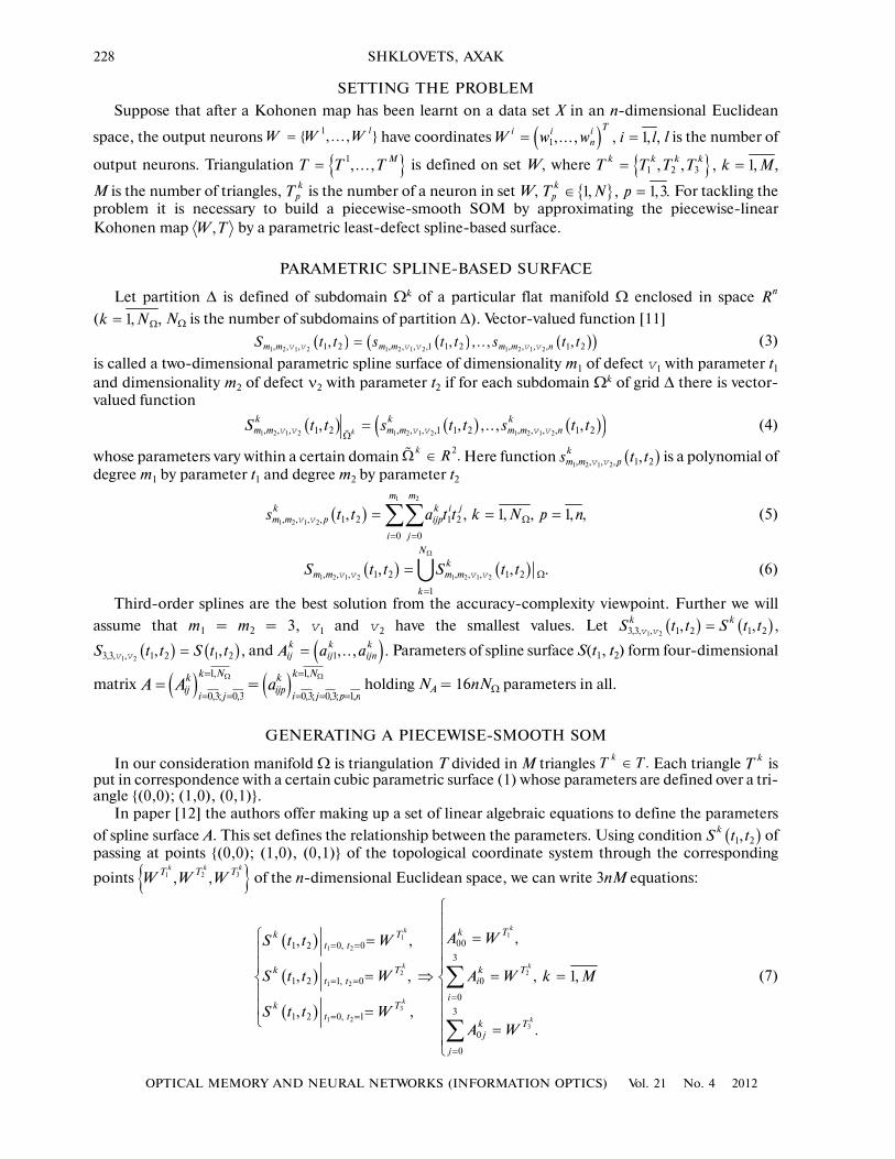
MAPPING HIGH�DIMENSIONAL DATA ONTO A PIECEWISE�SMOOTH KOHONEN MAP

It is seen from Figure 2 that the projection of the element point on a map formed as a para�metric spline surface is defined by solving the set of equations:

(13)

If we disclose the brackets in (13) and take (3)�(5) into account, we find that the first functions of set(13) are polynomials of the 5�th and 6�th order correspondingly, and the second functions polynomials ofthe 6�th and 5�th order with respect to variables t1 and t2. The Newton method with a few initial data is

offered to solve the set. The result of the mapping is set .The computational burden of the mapping of high�dimensional data on a piecewise�smooth Kohonen

map is linearly dependent on initial data.

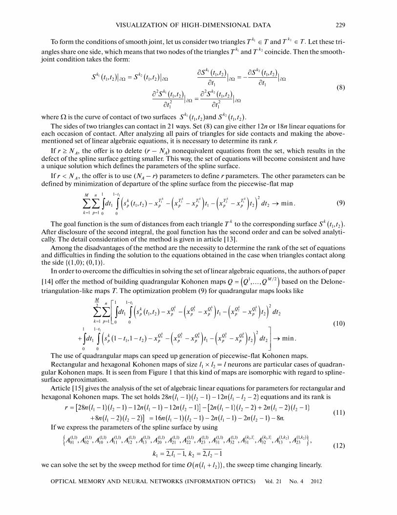
NUMERICAL EXPERIMENTS

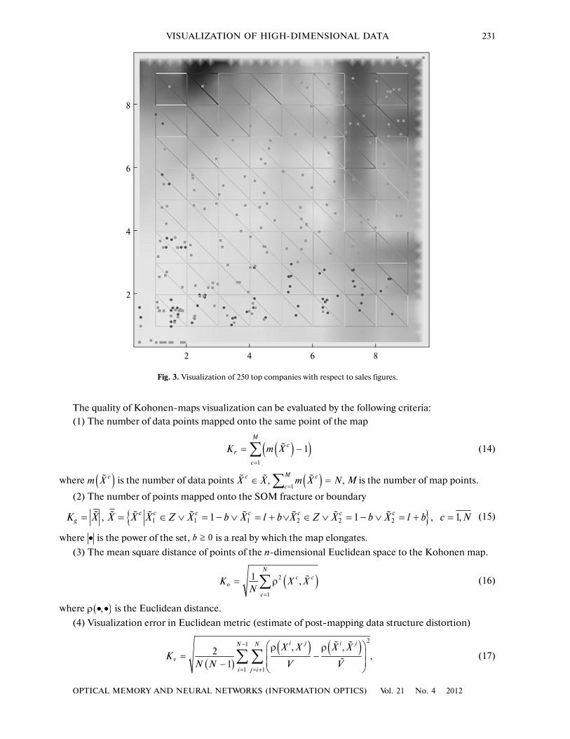
The analysis of the polymer market formed by CIS companies was done by visualization of datadescribed by such parameters as the name of a company, the state, the sort of polymer, the gain for the lastyear and month in tons and percent, the early and monthly share in imports in per cent, the early andmonthly imports in tons. Based on rectangular 9 × 9 piecewise�smooth SOMs, the visualization gave theresult shown in Figure 3. In the figure light square marks stand for Russian companies, dark round marksdenote Ukrainian companies (companies from other states did not enter the list). The stretching of themap in the high�dimensional space is shown as the background. It is seen from the figure that all the com�panies are divided in 4 classes with the majority of the companies being in one light cluster. The examina�tion shows that the right top cluster holds the companies with high values of almost all indicators. Theseare leading, exclusively Russian, companies. The left top corner has two companies that are away from theothers. These are novice companies which have increased their turnover.

cX X∈

( )1 2,S t t

( )( )( )

( )( )( )

1 21 2

1

1 21 2

2

,. , 0,

,. , 0,

c

c

S t tS t t X

t

S t tS t t X

t

∂⎧ − =⎪ ∂⎪⎨∂⎪ − =⎪ ∂⎩

1, .c N=

X�

Fig. 1. Rectangular and hexagonal 3 × 4 Kohonen maps.

∂Sk1

∂t2

Sk1(t1, t2)

∂Sk2

∂t2∂Sk2

∂t1

X c

Sk2(t1, t2)

Fig. 2. Mapping of element Xc on spline surface S(t1, t2).

OPTICAL MEMORY AND NEURAL NETWORKS (INFORMATION OPTICS) Vol. 21 No. 4 2012

VISUALIZATION OF HIGH�DIMENSIONAL DATA 231

The quality of Kohonen�maps visualization can be evaluated by the following criteria:(1) The number of data points mapped onto the same point of the map

(14)

where is the number of data points M is the number of map points.

(2) The number of points mapped onto the SOM fracture or boundary

(15)

where is the power of the set, is a real by which the map elongates.

(3) The mean square distance of points of the n�dimensional Euclidean space to the Kohonen map.

(16)

where is the Euclidean distance.

(4) Visualization error in Euclidean metric (estimate of post�mapping data structure distortion)

(17)

( )( )1

1M

cr

c

K m X=

= −∑ �

( )cm X� ,cX X∈� � ( )1

,M c

cm X N

=

=∑ �

{ }1 1 1 2 2 2, 1 1 , 1,c c c c c c cgK X X X X Z X b X l b X Z X b X l b c N= = ∈ ∨ = − ∨ = + ∨ ∈ ∨ = − ∨ = + =

� � � � � � � � �

• 0b ≥

( )2

1

1 ,N

c co

c

K X XN

=

= ρ∑ �

( ),ρ • •

( )

( ) ( ) 21

1 1

, ,2 ,1

i j i jN N

v

i j i

X X X XK

N N V V

−

= = +

⎛ ⎞ρ ρ⎜ ⎟= −⎜ ⎟− ⎝ ⎠

∑∑� �

�

2

2

4 6 8

4

6

8

Fig. 3. Visualization of 250 top companies with respect to sales figures.

232

OPTICAL MEMORY AND NEURAL NETWORKS (INFORMATION OPTICS) Vol. 21 No. 4 2012

SHKLOVETS, AXAK

where

(18)

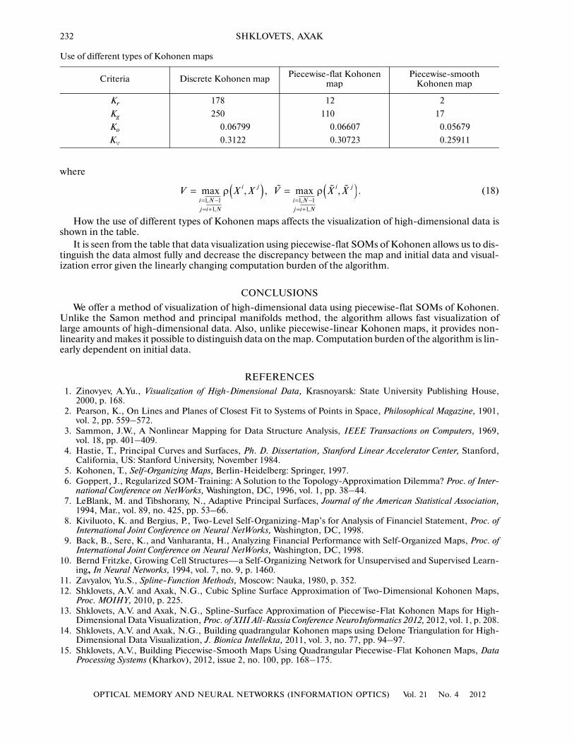
How the use of different types of Kohonen maps affects the visualization of high�dimensional data isshown in the table.

It is seen from the table that data visualization using piecewise�flat SOMs of Kohonen allows us to dis�tinguish the data almost fully and decrease the discrepancy between the map and initial data and visual�ization error given the linearly changing computation burden of the algorithm.

CONCLUSIONS

We offer a method of visualization of high�dimensional data using piecewise�flat SOMs of Kohonen.Unlike the Samon method and principal manifolds method, the algorithm allows fast visualization oflarge amounts of high�dimensional data. Also, unlike piecewise�linear Kohonen maps, it provides non�linearity and makes it possible to distinguish data on the map. Computation burden of the algorithm is lin�early dependent on initial data.

REFERENCES

1. Zinovyev, A.Yu., Visualization of High�Dimensional Data, Krasnoyarsk: State University Publishing House,2000, p. 168.

2. Pearson, K., On Lines and Planes of Closest Fit to Systems of Points in Space, Philosophical Magazine, 1901,vol. 2, pp. 559–572.

3. Sammon, J.W., A Nonlinear Mapping for Data Structure Analysis, IEEE Transactions on Computers, 1969,vol. 18, pp. 401–409.

4. Hastie, T., Principal Curves and Surfaces, Ph. D. Dissertation, Stanford Linear Accelerator Center, Stanford,California, US: Stanford University, November 1984.

5. Kohonen, T., Self�Organizing Maps, Berlin�Heidelberg: Springer, 1997.6. Goppert, J., Regularized SOM�Training: A Solution to the Topology�Approximation Dilemma? Proc. of Inter�

national Conference on NetWorks, Washington, DC, 1996, vol. 1, pp. 38–44.7. LeBlank, M. and Tibshorany, N., Adaptive Principal Surfaces, Journal of the American Statistical Association,

1994, Mar., vol. 89, no. 425, pp. 53–66.8. Kiviluoto, K. and Bergius, P., Two�Level Self�Organizing�Map’s for Analysis of Financiel Statement, Proc. of

International Joint Conference on Neural NetWorks, Washington, DC, 1998.9. Back, B., Sere, K., and Vanharanta, H., Analyzing Financial Performance with Self�Organized Maps, Proc. of

International Joint Conference on Neural NetWorks, Washington, DC, 1998.10. Bernd Fritzke, Growing Cell Structures—a Self�Organizing Network for Unsupervised and Supervised Learn�

ing, In Neural Networks, 1994, vol. 7, no. 9, p. 1460.11. Zavyalov, Yu.S., Spline�Function Methods, Moscow: Nauka, 1980, p. 352.12. Shklovets, A.V. and Axak, N.G., Cubic Spline Surface Approximation of Two�Dimensional Kohonen Maps,

Proc. MOIHY, 2010, p. 225.13. Shklovets, A.V. and Axak, N.G., Spline�Surface Approximation of Piecewise�Flat Kohonen Maps for High�

Dimensional Data Visualization, Proc. of XIII All�Russia Conference NeuroInformatics 2012, 2012, vol. 1, p. 208.14. Shklovets, A.V. and Axak, N.G., Building quadrangular Kohonen maps using Delone Triangulation for High�

Dimensional Data Visualization, J. Bionica Intellekta, 2011, vol. 3, no. 77, pp. 94–97.15. Shklovets, A.V., Building Piecewise�Smooth Maps Using Quadrangular Piecewise�Flat Kohonen Maps, Data

Processing Systems (Kharkov), 2012, issue 2, no. 100, pp. 168–175.

( ) ( )1, 1 1, 1

1, 1,

max , , max , .i j i j

i N i N

j i N j i N

V X X V X X= − = −

= + = +

= ρ = ρ� � �

Use of different types of Kohonen maps

Criteria Discrete Kohonen map Piecewise�flat Kohonen map

Piecewise�smooth Kohonen map

Kr 178 12 2

Kg 250 110 17

Ko 0.06799 0.06607 0.05679

Kv

0.3122 0.30723 0.25911