visualizing and understanding code duplication in large
TRANSCRIPT
Visualizing and Understanding Code
Duplication in Large Software Systems
by
Zhen Ming Jiang
A thesis
presented to the University of Waterloo
in fulfillment of the
thesis requirement for the degree of
Master of Mathematics
in
Computer Science
Waterloo, Ontario, Canada, 2006
c©Zhen Ming Jiang, 2006

Authors Declaration for Electronic Submission of a Thesis
I hereby declare that I am the sole author of this thesis. This is a true copy of the thesis,
including any required final revisions, as accepted by my examiners.
I understand that my thesis may be made electronically available to the public.
ii
Abstract
Code duplication, or code cloning, is a common phenomena in the development of large
software systems. Developers have a love-hate relationship with cloning. On one hand,
cloning speeds up the development process. On the other hand, clone management is a
challenging task as software evolves. Cloning has commonly been considered as undesirable
for software maintenance and several research efforts have been devoted to automatically
detect clones and eliminate clones aggressively. However, there is little empirical work done
to analyze the consequences of cloning with respect to the software quality. Recent studies
show that cloning is not necessarily undesirable. Cloning can used to minimize risks and
there are cases where cloning is used as a design technique.
In this thesis, three visualization techniques are proposed to aid researchers in ana-
lyzing cloning in studying large software systems. All of the visualizations abstract and
display cloning information at the subsystem level but with different emphases. At the
subsystem level, clones can be classified as external clones and internal clones. External
clones refer to code duplicates that reside in the same subsystem, whereas external clones
are clones that are spread across different subsystems. Software architecture quality at-
tributes such as cohesion and coupling are introduced to contribute to the study of cloning
at the architecture level. The Clone Cohesion and Coupling (CCC) Graph and the Clone
System Hierarchy (CSH) Graph display the cloning information for one single release. In
particular, the CCC Graph highlights the amount of internal and external cloning for each
subsystems; whereas the CSH Graph focuses more on the details of the spread of cloning.
Finally, the Clone System Evolution (CSE) Graph shows the evolution of cloning over a
period of time.
iii

Acknowledgements
This thesis would not have been possible without the continuous support of my parents
who always support me and give me will to succeed.
I would like to thank my supervisor Dr. Richard C. Holt for his support and advice.
A special thank you to Dr. Ahmed E. Hassan for his fruitful suggestion and constant
motivation throughout my research career both as a undergraduate research assistant and
as a graduate student. I also thank him for offering me the opportunity to visit University
of Victoria in the summer. That is a very enjoyable experience.
In addition, I appreciate the valuable feedback provided by two of my thesis readers:
Dr Michael Godfrey and Dr. Joanne Atlee.
I am very fortunate to work with the amazing members of SWAG. In particular, I would
like to thank Cory Kapster, Abram Hindle, LiJie Zou, and Olga Baysal for all their help
and encouragement.
Finally, I thank for all my friends who patiently put up with me while I worked away
on my thesis.
iv
Contents
1 Introduction 1
1.1 Code Cloning . . . . . . . . . . . . . . . . . . . . . . . . . . . . . . . . . . 1
1.1.1 Why Do People Clone Source Code? . . . . . . . . . . . . . . . . . 5
1.1.2 Why Should People Not Clone Source Code? . . . . . . . . . . . . . 7
1.1.3 Challenge of Dealing with Clones . . . . . . . . . . . . . . . . . . . 8
1.2 Overview of Thesis . . . . . . . . . . . . . . . . . . . . . . . . . . . . . . . 8
1.2.1 Scaling . . . . . . . . . . . . . . . . . . . . . . . . . . . . . . . . . . 9
1.2.2 Visualization . . . . . . . . . . . . . . . . . . . . . . . . . . . . . . 14
1.3 Major Thesis Contributions . . . . . . . . . . . . . . . . . . . . . . . . . . 15
1.4 Thesis Organization . . . . . . . . . . . . . . . . . . . . . . . . . . . . . . . 16
2 Clone Data Extraction 18
2.1 Summary of Clone Detection Techniques . . . . . . . . . . . . . . . . . . . 18
2.2 Data Generation and Pre-Processing . . . . . . . . . . . . . . . . . . . . . 19
2.2.1 Automatic Clone Data Detection . . . . . . . . . . . . . . . . . . . 20
2.2.2 Clone Data Filtering . . . . . . . . . . . . . . . . . . . . . . . . . . 20
3 Related Work 27
vi
3.1 Clone Visualization . . . . . . . . . . . . . . . . . . . . . . . . . . . . . . . 27
3.2 Clone Evolution . . . . . . . . . . . . . . . . . . . . . . . . . . . . . . . . . 31
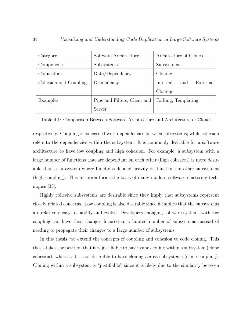
4 Clone Cohesion and Coupling (CCC) Graph 32
4.1 Architecture of Clones . . . . . . . . . . . . . . . . . . . . . . . . . . . . . 33
4.2 Our Approach . . . . . . . . . . . . . . . . . . . . . . . . . . . . . . . . . . 35
4.2.1 Clone Architecture Recovery Framework . . . . . . . . . . . . . . . 36
4.2.2 Clone Cohesion and Coupling (CCC) Graph . . . . . . . . . . . . . 40
4.3 Case Study: The Clone Architecture of SCSI Subsystem . . . . . . . . . . 44
4.3.1 Results of Our Clone Extraction Framework . . . . . . . . . . . . . 45
4.3.2 Subsystem Mapping . . . . . . . . . . . . . . . . . . . . . . . . . . 45
4.3.3 Clone Cohesion and Coupling (CCC) Graph . . . . . . . . . . . . . 47
4.4 Usage Guideline . . . . . . . . . . . . . . . . . . . . . . . . . . . . . . . . . 49
4.5 Conclusion . . . . . . . . . . . . . . . . . . . . . . . . . . . . . . . . . . . . 51
5 Clone System Hierarchical(CSH) Graph 52
5.1 Clone System Hierarchy Extraction Framework . . . . . . . . . . . . . . . 54
5.2 Clone System Hierarchical (CSH) Graph . . . . . . . . . . . . . . . . . . . 57
5.2.1 Sub-View 1: Static View . . . . . . . . . . . . . . . . . . . . . . . . 58
5.2.2 Sub-View 2: Pointing and Clicking View . . . . . . . . . . . . . . . 60
5.2.3 Sub-View 3: Animation View . . . . . . . . . . . . . . . . . . . . . 66
5.3 Discussion and Future Work . . . . . . . . . . . . . . . . . . . . . . . . . . 68
5.4 Usage Guideline . . . . . . . . . . . . . . . . . . . . . . . . . . . . . . . . . 70
5.5 Conclusion . . . . . . . . . . . . . . . . . . . . . . . . . . . . . . . . . . . . 71
6 Clone System Evolution (CSE) Graph 72
6.1 Software Evolution . . . . . . . . . . . . . . . . . . . . . . . . . . . . . . . 73
vii
6.1.1 Our Methodology . . . . . . . . . . . . . . . . . . . . . . . . . . . . 75
6.1.2 Examining the Evolution of Linux using ULOC . . . . . . . . . . . 76
6.1.3 An Alternative . . . . . . . . . . . . . . . . . . . . . . . . . . . . . 80
6.1.4 Discussion . . . . . . . . . . . . . . . . . . . . . . . . . . . . . . . . 81
6.2 Clone System Evolutionary (CSE) Graph . . . . . . . . . . . . . . . . . . . 82
6.2.1 Clone System Evolution Framework . . . . . . . . . . . . . . . . . . 83
6.2.2 Clone System Evolutionary (CSE) Graph . . . . . . . . . . . . . . . 85
6.2.3 An Example . . . . . . . . . . . . . . . . . . . . . . . . . . . . . . . 86
6.2.4 Discussion and Future Work . . . . . . . . . . . . . . . . . . . . . . 89
6.3 Guideline . . . . . . . . . . . . . . . . . . . . . . . . . . . . . . . . . . . . 91
6.4 Conclusion . . . . . . . . . . . . . . . . . . . . . . . . . . . . . . . . . . . . 92
7 Conclusion and Future Work 93
7.1 Major Topics Addressed . . . . . . . . . . . . . . . . . . . . . . . . . . . . 94
7.2 Future Research . . . . . . . . . . . . . . . . . . . . . . . . . . . . . . . . . 94
viii
List of Tables
2.1 Number of Clone Pairs Before and After Filtering for Linux Kernel. . . . . 24
3.1 Summary of Clone Visualization Tools . . . . . . . . . . . . . . . . . . . . 29
4.1 Comparison Between Software Architecture and Architecture of Clones . . 34
4.2 Description of the Dimensions of Nodes . . . . . . . . . . . . . . . . . . . . 41
5.1 The Actions and Effects for the Pointing Mode . . . . . . . . . . . . . . . . 61
5.2 The Actions and Effects for the Clicking Mode . . . . . . . . . . . . . . . . 64
ix
List of Figures
1.1 Clone example taken from Linux Kernel version 2.6.16.13. . . . . . . . . . 2
1.2 An example of clone pairs. . . . . . . . . . . . . . . . . . . . . . . . . . . . 3
1.3 An example of clone classes. . . . . . . . . . . . . . . . . . . . . . . . . . . 4
1.4 Clone classes before merging. . . . . . . . . . . . . . . . . . . . . . . . . . 10
1.5 Clone classes after merging. . . . . . . . . . . . . . . . . . . . . . . . . . . 11
1.6 Clone classes before lifting. . . . . . . . . . . . . . . . . . . . . . . . . . . . 12
1.7 Clone classes after lifting. . . . . . . . . . . . . . . . . . . . . . . . . . . . 13
2.1 Structural Filtering . . . . . . . . . . . . . . . . . . . . . . . . . . . . . . . 25
3.1 Comparison between two approaches . . . . . . . . . . . . . . . . . . . . . 30
4.1 Our Clone Architecture Recovery Framework. . . . . . . . . . . . . . . . . 37
4.2 Schemas Used in Our Framework. . . . . . . . . . . . . . . . . . . . . . . . 38
4.3 Heat Coloring. . . . . . . . . . . . . . . . . . . . . . . . . . . . . . . . . . . 42
4.4 An Example of the Clone Cohesion and Coupling (CCC) graph. . . . . . . 43
4.5 Annotated Screenshots of the CCC graph for the Linux SCSI drivers. . . . 48
5.1 Our Clone System Hierarchy Extraction Framework. . . . . . . . . . . . . 55
5.2 Schemas Used in Our Framework. . . . . . . . . . . . . . . . . . . . . . . . 56
x
5.3 Annotated Screenshots of the CSH Graph for Linux Kernel 1.0. . . . . . . 58
5.4 Screenshots of Static View of CSH Graph for Linux Kernel 1.0. . . . . . . . 59
5.5 Pointing and Clicking View of CSH Graph for Linux Kernel 1.0. . . . . . . 62
5.6 Another Pointing and Clicking View of CSH Graph for Linux Kernel 1.0. . 65
5.7 Animation View of CSH Graph for Linux Kernel 1.0. . . . . . . . . . . . . 67
6.1 SLOC and ULOC plots for Linux stable releases . . . . . . . . . . . . . . . 77
6.2 SLOC and ULOC plots for top level directories Linux stable releases . . . . 79
6.3 Plot of Compressed tar.gz File sizes for Linux stable releases. . . . . . . . . 80
6.4 Clone Evolutionary Extraction Framework. . . . . . . . . . . . . . . . . . . 84
6.5 The CSE graph for 9 releases of Linux Kernel. . . . . . . . . . . . . . . . . 86
6.6 The CSE graph for drivers subsystem in 9 Linux Kernel releases. . . . . . . 86
6.7 The Clone Difference Between Linux 2.6 and 2.6.16.13. . . . . . . . . . . . 88
xi
Chapter 1
Introduction
Clones are identical or near identical segments of source code. Code clones are usually
intentionally created through copying another piece of code. However, in certain cases [35]
clones appears unintentionally due to code segments using the same APIs. Code cloning
is a common phenomena in the development of large software systems. It is reported that
5-50% of large software systems are clones [8, 39, 7].
This chapter consists of the following parts: Section 1.1 provides a background of code
cloning. Section 1.2 gives an overview of the thesis. Section 1.3 briefly discusses the
novelties of this thesis. Section 1.4 talks about the organization of the thesis.
1.1 Code Cloning
A clone is a segment of code that has been created through duplication of another piece
of code. Clones share similar code structures. However, since the size and the degree
of similarities among code segments vary, code cloning is a fairly subjective concept. It
depends on the context or human judgement whether it is a code clone or not.
1
2 Visualizing and Understanding Code Duplication in Large Software Systems
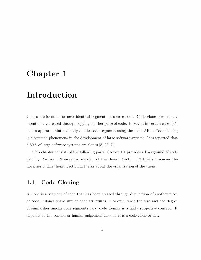
Figure 1.1: Clone example taken from Linux Kernel version 2.6.16.13.
Figure 1.1 shows an example of code cloning drawn from the Linux Kernel. The source
code is taken from the code responsible for supporting the different network cards in
the Linux Kernel version 2.6.16.13. The top row shows the file names and line numbers
separated by colons. Areas highlighted in grey indicates the code duplication sections and
the red font marks variation points.
When referring to clone relations, we use two terms: clone pairs and clone classes. A
clone pair is a pair of code segments which are identical or similar to each other. A clone
class is the maximum set of code segments in which any two of the code segments forms
a clone pair. For example, A, B, C is a clone class. It implies that we have clone pairs
(A, B), (B, C), and (C, A).
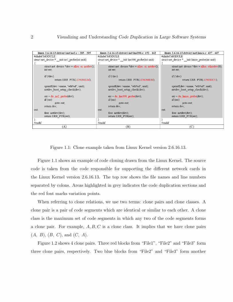
Figure 1.2 shows 4 clone pairs. Three red blocks from “File1”, “File2” and “File3” form
three clone pairs, respectively. Two blue blocks from “File2” and “File3” form another
Introduction 3
Figure 1.2: An example of clone pairs.

4 Visualizing and Understanding Code Duplication in Large Software Systems
Figure 1.3: An example of clone classes.
Introduction 5
clone pair. Figure 1.2 shows the same cloning data by using clone classes relations. It has
two clone classes: a pink diamond indicating the clone class connecting three red blocks;
and a blue diamond representing another clone class connecting two blue blocks.
The rest of this section is organized as follows. First, we talk about intentions why
developers clone source code. Then we discuss reasons why developers should not clone
source code. Finally, we present a few challenges of managing code clones.
1.1.1 Why Do People Clone Source Code?
There are a number of reasons why developers clone source code [36, 8, 32]. Here we
summarize a few common scenarios.
Code cloning is unavoidable due to language limitations. For example, Standard
Template Library(STL) in C++ is considered as a typical example of genericity.
However, Basit et. al. [20] showed that there are still code duplications which cannot
be eliminated by using generic programming language features such as templates.
Code cloning is used for reusing certain design patterns. For example, Cordy [22]
pointed out from his years of experience in dealing with financial software systems
that cloning is “the way in which designs are reused in these systems”. He observed
that there are only a limited number of tasks in the finance field; therefore the
data structure and data manipulation operations are quite similar to each other.
Consequently, whenever there is a need to write a new module; it is considered
common practice to copy from the old code, which is trusted and tested.
Code cloning is adopted to preserve performance. For example, in real-time appli-
cations, some common operations are hand-optimized to achieve best performance.
6 Visualizing and Understanding Code Duplication in Large Software Systems
It is required to copy from the existing optimized code whenever the same operations
is needed.
Code cloning is used for experimentation purposes. It is discovered that [32] when
developers start implementing new features they tend to copy from existing code. As
they gain a deeper understanding of the problem and think more about the solution;
these clones will be eliminated.
Code cloning is used for templating. For example, drivers are code written to enable
operating systems to interact with hardware devices. Driver code is considered as
the main source of errors in operating system [2]. What is more, it is fairly mechanic
to write drivers. To implement a Linux SCSI driver [3], we need to implement only a
few specified functions, and set these functions to point to appropriate fields for one
struct. Rather than writing driver code from scratch, which is time-consuming and
error-prone, it is preferable to copy from an existing driver code and modify it.
Code cloning is used in cross-cutting concerns. Code segments for error-checking
or logging are usually scattered across the code base [30]. Developers clone error-
checking or logging code to preserve consistency of the coding style.
Code cloning is used for risk minimization. Cordy [22] and Kapster [11] observed
that rather than abstracting out the common operations, copying well-tested code
reduces the risks of either breaking existing functionality as well as isolating the risks
of introducing software defects to a single place.
Academically, there are studies [32, 27, 11] showing that cloning is considered a common
practice in the software development process. There are quite a few cases when clone is
used as a design pattern and are considered beneficial. For example, the forking patterned
Introduction 7
mentioned in [11] can be used to test new features without affecting existing functionality.
Therefore, there is a need to develop various kinds of clone maintenance tools [11].
1.1.2 Why Should People Not Clone Source Code?
Many researchers believe that cloning is a “bad smell” for code quality as it brings up
challenges for software maintenance.
• Code cloning leads to a bloated code base. This leads to a large binary executables
and requires more storage spaces. In devices that have limited storage spaces such
as cell-phones, the amount of cloning has to be minimized.
• Code cloning causes additional effort for developers. As clone instances are similar
to each other, developers need to careful examine the two pieces of code in order to
tell the differences among clone instances.
• Code cloning brings challenges to software maintenance. When developers modify
one clone piece apart(usually for bug fixes), it is very likely that they need to apply
the same changes to its cloning instances. Therefore,
– developers need to check all its cloning instances to decide whether similar
changes need to be applied on them, and
– uncover cloning information is hard, since cloning knowledge is usually left as
undocumented and only exists in developers’ head as short term memory.
Based on this brief, tools have been developed to automatically detect clones [25, 28, 8]
and techniques have been proposed to automatically eliminate clones [16, 34].
8 Visualizing and Understanding Code Duplication in Large Software Systems
1.1.3 Challenge of Dealing with Clones
Code cloning is a common practice in the software development, yet the long term effects are
not well-understood. As we have shown in Sections 1.1.1 and 1.1.2, there are two opposing
views towards code cloning. These two views examine clones from different perspectives
and are both tenable. Unfortunately, to date there has been only one empirical study done
to study the consequence of cloning [4].
A major problem of conducting clone studies in a large software system is how do
handle large volume of data. Code clones are quite common in large software systems.
Software systems such as Linux Kernel, which has several million lines of source code, may
contain thousands of lines of clones.
The goal of this thesis is to develop tools and techniques to aid researchers to analyze
code cloning in large software systems.
Our approach uses scaling and visualizing. We scale the huge volume of cloning data by
three techniques: merging clone classes into bigger clone classes, lifting cloning relations
from code segment level to file level or subsystem level, and pruning irrelevant cloning
relations. Then we visualize our data along three dimensions: amount, spread, and time.
The overview of the thesis is presented in Section 1.2.
1.2 Overview of Thesis
In this thesis, we propose tools and techniques to help researchers to understand code
cloning in large software systems. We accomplish this by providing visualizations which
support large data set.
We scale down the cloning data by providing various levels of abstractions and then
provide three visualization techniques to highlight cloning along three different dimensions.
Introduction 9
1.2.1 Scaling
We achieve scaling by three techniques: merging, lifting and filtering. We detail the scaling
process as follows:
Merging: Each clone class obtained from the clone detection tools contains the line
interval which are duplicates. Different clone classes can have the same files but
with different line intervals. If two clone classes contain exactly the same files or
subsystems, then we merge these clone classes into one bigger clone class.
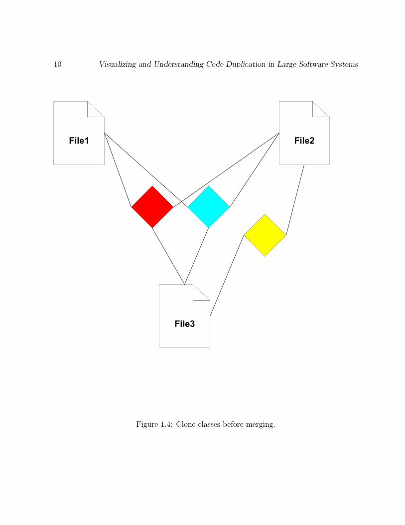
We are going to illustrate this by means of an example. Figure 1.4 shows the clone
classes before merging. We have three clone classes: the red, the blue and the yellow
clone classes. Both the red clone class and the blue clone class contain three files;
whereas the yellow clone class only contains 2 files. Figure 1.5 shows the clone classes
after merging. We have two clone classes: the grey clone class, which is the result of
merging the red and the blue clone classes; and the yellow clone class stays the same
since it only contains 2 files and cannot be merge with the other two clone classes
which both contain three files.
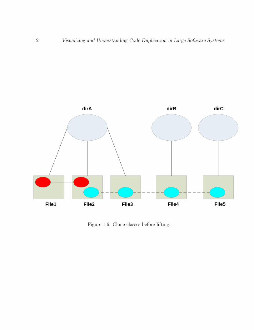
Lifting: The lifting step elevates cloning relations from the code segment level to the
file level or up to the subsystem level.
We will illustrate the lifting process by means of an example. Figure 1.6 shows the
cloning relations before lifting. We have three directories: “dirA”, “dirB” and “dirC”.
Under “dirA”, we have three files: “File1”, “File2” and “File3”; under “dirB”, we
have 1 file: “File4”; and under “dirC”, we have 1 file: “File5”. We have 2 clone
classes: one clone classes contains code segments shown in red and one clone classes
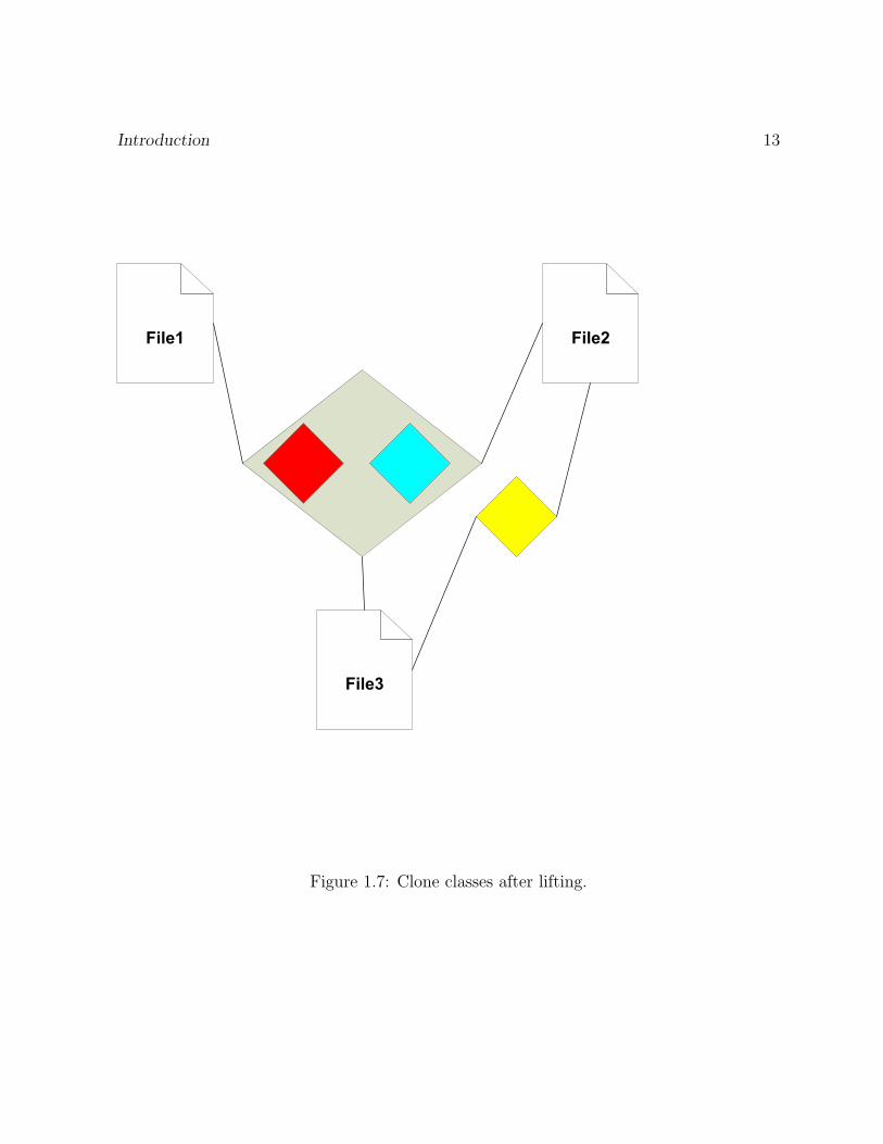
contains code segments shown in blue. Figure 1.7 shows the result after lifting. Since
“File1” and “File2” are both under “dirA”, therefore the red clone class gets lifted to
10 Visualizing and Understanding Code Duplication in Large Software Systems
Figure 1.4: Clone classes before merging.

Introduction 11
Figure 1.5: Clone classes after merging.
12 Visualizing and Understanding Code Duplication in Large Software Systems
File1 File2 File3 File4 File5
dirA dirB dirC
Figure 1.6: Clone classes before lifting.
Introduction 13
Figure 1.7: Clone classes after lifting.
14 Visualizing and Understanding Code Duplication in Large Software Systems
“dirA”, one blue block in “dirA” is from “File3”. Similary, all the cloning relations
from “File4” and “File5” are lifted to “dirB” and “dirC”, respectively.
Pruning: Depending on the study we focus on, irreverent cloning data can be selec-
tively removed. For example, if we are only interested in cloning related to “drivers”
subsystem; then we can remove all the clone classes which do not contain files in
“drivers”. If we are only interested in cloning relations among subsystems, then we
can remove all the file level cloning relations.
We name the resulting clone classes after merging and lifting steps as Super Clone
Classes.
Note that merging and lifting steps can be used at any levels of system abstraction. In
addition, the ordering of executing merging and lifting actions does not really matter.
For example, if we want the data to be scaled at the file level, we can first lift the clone
classes at the code segment level first to the subsystem level and then merge the lifted
clone classes. Alternatively, at the code segment level we can choose to merge clone classes
that contain exactly the same set of files, then we lift them to the file level. The results
will be the same.
Similarly, if we want the data to be scaled at the lowest subsystem level, we can first
merge clone classes which associate with exactly the same lowest level subsystems, then
we lift the clone classes into the lowest subsystem level, or the other way around.
1.2.2 Visualization
Three visualization techniques are proposed in this thesis. Each of them emphasizes cloning
along different dimensions: quantity, spread and time, respectively. Quantity refers to
how much duplications within one subsystem (internal cloning) and between subsystems
Introduction 15
(external cloning). Spread refers to the details of cloning relations; that is how many
subsystems or files it cross-cut. Time refers to how clones evolve over time in different
parts of the subsystem.
Quantity: The Clone Cohesion and Coupling (CCC) Graph displays the amount of
cloning that exists within one subsystem (internal cloning) as well as the the amount
of cloning that exists between subsystems (external cloning).
It highlights the amount of code duplication between subsystems.
Spread: The Clone System Hierarchical (CSH) Graph lays out the cloning data in the
system hierarchical structure.
It highlights cloning relations for individual files and directories by mouse movements.
It emphasize the spread of cloning.
Time: The Clone System Evolution (CSH) Graph visualizes the evolvement of clones
over time.
It highlights the most recent changes of code cloning.
1.3 Major Thesis Contributions
In this thesis, we introduce the concept of “Architecture of Clones” to help researchers to
understand large set of cloning data. The concepts of cohesion and coupling are applied
in the context of cloning to evaluate the quality of the software systems.
Three visualization techniques are proposed to help researchers to better understand
large set of cloning data.
16 Visualizing and Understanding Code Duplication in Large Software Systems
• The CCC graph is the first attempt to use energy-based graph layout to visualize the
strength of external cloning among subsystems. Super clones scale the studies; what
is more, visualization clone classes rather than pairs reduces the cross-cutting edges.
• The CSH graph lays out clone information in the hierarchy containment structure
highlighting the spread of cloning. It also provides mechanisms to allow researchers
to interactively query clone relations for each subsystem.
• The CSE graph shows the evolution of architecture of clones over time.
• For each of the three of the visualizations proposed in this thesis, we provide a
guideline that summarizes how to reconstruct our visualizations. This is useful for
researchers who are interested in using our tools to analyze cloning for other software
systems.
• All three graphs covey the information of clone cohesion and coupling in the large
software systems. They can also be applied to other areas of research like co-change.
In addition, two data filtering techniques are introduced and compared to remove false
clones.
Finally, the metric uloc is a new metric to study the growth rate of the software systems.
1.4 Thesis Organization
The rest of this thesis is organized as follows: Chapter 2 shows how we obtain the cloning
data set. Chapter 3 presents related research. Chapter 4 presents the first of our three
clone visualizations: the Clone Cohesion and Coupling( CCC) graph. Chapter 5 explains
the second visualization technique: the Clone System Hierarchical (CSH) graph. Chapter 6

Introduction 17
introduces the concept of uloc and the third visualization: Clone System Evolution (CSE)
graph. Finally, Chapter 7 summarizes our work and presents some future work.
Chapter 2
Clone Data Extraction
This chapter explains the steps used to extract the cloning data from a large software
system. It is organized as follows: Section 2.1 explains the current existing clone detection
techniques. Section 2.2 explains our choice of clone detection tool and techniques to remove
inappropriate clones.
2.1 Summary of Clone Detection Techniques
There are four general techniques to detect clones:
Metrics Analysis: Metric-based clone detection techniques [28] collect various metrics
such as: McCabe’s Cyclomatic complexity, number of passed parameters, number of
used/defined local/global variables, etc. Depending on how similar these metrics are,
various code segments may be marked as clones. This approach is fast to compute,
but it lacks precision. It is recommended to be used for pre-processing step to narrow
down the selection of files that are going to be processed for more finely grained clone
detection.
18
Clone Data Extraction 19
Simple Text Comparison: Simple text comparison techniques locate exact matches
of code segments. The Exact Match Clone Detection algorithm described in [14] is
an example of such a technique. The algorithm normalizes the code by removing
comments and suppressing white spaces. It then tries to find all matched lines for
each line. The algorithm uses a pattern matching algorithm to generate a list of
maximal number of consecutive lines of cloned code for each code segment. Finally,
cloning results are generated by filtering out smaller code segments. For the example
shown in Figure 1.1, a simple text comparison technique would not recognize the
variation points (in red). Instead of identifying a single large clone code segment,
the algorithm would identify several smaller code segments as clones.
Lexical Analysis: Lexical analysis techniques tokenize the code and concatenate tokens
into token sequences. Then they create abstract token strings to mark identifers and
code constructs. The abstract token strings are used to locate maximal substring
matches. An example of a tool that uses such a technique is the CCFinder tool [25].
The example shown in Figure 1.1 was identified by CCFinder.
AST Analysis: Abstract Syntax Tree (AST) Analysis techniques parse the code and
create an abstract syntax tree. The techniques then compare AST subtrees. Clones
are detected if two subtrees are identical to each other. An example of such a tech-
nique is presented in [5]. The example shown in Figure 1.1 would be identified by
such techinques.
2.2 Data Generation and Pre-Processing
This section describes how we pre-process the data used for our visualizations. It consists
of two steps: automatic detecting clone data and removing false clones.
20 Visualizing and Understanding Code Duplication in Large Software Systems
2.2.1 Automatic Clone Data Detection
We use the CCFinder [25] as our clone detection tool. CCFinder is a lexical-analysis-type
clone detection tool. It uses“Parameterized String Matching” algorithm to extract clone
pairs and is reported to have a high recall rate compared to other tools [9].
In order to reduce the reporting of rather small trivial clones, CCFinder must be con-
figured with a minimum clone size. We chose 30 tokens as the minimum clone size, since
previous studies [27, 26] show that the output of CCFinder is of reasonable accuracy at
this token level. We also turn off the option to locate clones within the same file, since we
are more interested in detecting similarities across source code files and subsystems at the
architecture level. Different options can be configured and other clone detection tools can
be used if needed.
CCFinder output the clone detection results both in the form of clone pairs and clone
classes.
2.2.2 Clone Data Filtering
Through a manual analysis of the CCFinder output, we discovered that CCFinder occa-
sionally produces inappropriate cloning relations.
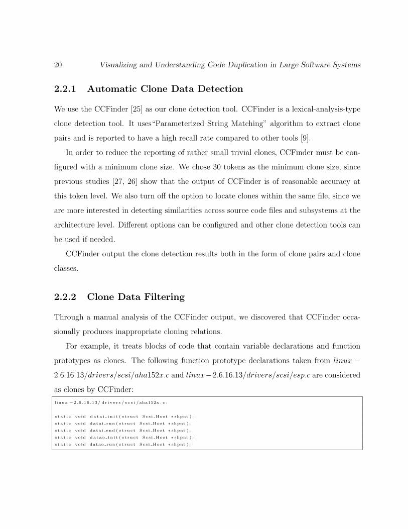
For example, it treats blocks of code that contain variable declarations and function
prototypes as clones. The following function prototype declarations taken from linux −
2.6.16.13/drivers/scsi/aha152x.c and linux−2.6.16.13/drivers/scsi/esp.c are considered
as clones by CCFinder:
l inux −2 .6 .16 .13/ d r i v e r s / s c s i /aha152x . c :
s t a t i c void d a t a i i n i t ( s t r u c t Sc s i Hos t ∗ shpnt ) ;
s t a t i c void data i run ( s t r u c t Sc s i Hos t ∗ shpnt ) ;
s t a t i c void data i end ( s t r u c t Sc s i Hos t ∗ shpnt ) ;
s t a t i c void d a t a o i n i t ( s t r u c t Sc s i Hos t ∗ shpnt ) ;
s t a t i c void datao run ( s t r u c t Sc s i Hos t ∗ shpnt ) ;
Clone Data Extraction 21
l inux −2 .6 .16 .13/ d r i v e r s / s c s i / esp . c :
s t a t i c i n t e sp do phase dete rmine ( s t r u c t esp ∗ esp ) ;
s t a t i c i n t e s p d o da t a f i n a l e ( s t r u c t esp ∗ esp ) ;
s t a t i c i n t e s p s e l e c t c omp l e t e ( s t r u c t esp ∗ esp ) ;
s t a t i c i n t e sp do s t a tu s ( s t r u c t esp ∗ esp ) ;
s t a t i c i n t esp do msgin ( s t r u c t esp ∗ esp ) ;
To remove the inappropriate clone relations reported by CCFinder, we have developed
two filtering techniques: Structural Filtering and Textual Filtering.
• Structural Filtering
We call cloned code segments that are not inside a function “non-functional clones”.
In the above example, the reported cloned segments are inside the variable declaration
block and these false positives are due to similar structures in variable declarations.
Therefore, we choose to remove non-functional clones to eliminate inappropriate clone
relations caused by variable declarations.
The filtering is accomplished by a Perl script. The script invokes a source code
tagging tool, called ctags [13] then parses the file to determine the beginning and
ending lines of all defined code entities such as functions, variables, macros, and
prototypes. The script then removes all identified CCFinder clone pairs which are
non-functional clones.
• Textural Filtering
Although structural filtering allows us to remove the non-functional clones caused
by variable declarations, it cannot filter out false positives caused by similarities in
program constructs.
For example, the format for case switch statement is usually one case statement
followed by one line of method invocation and then the break statement. The two
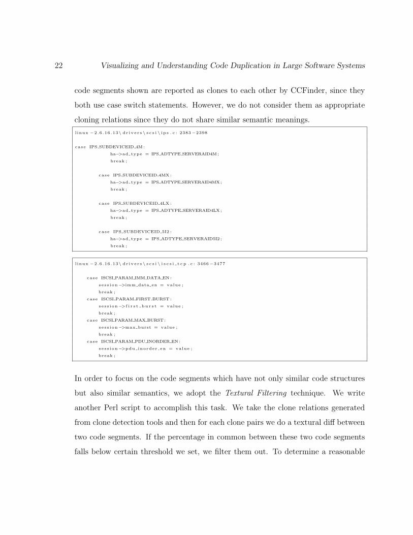
22 Visualizing and Understanding Code Duplication in Large Software Systems
code segments shown are reported as clones to each other by CCFinder, since they
both use case switch statements. However, we do not consider them as appropriate
cloning relations since they do not share similar semantic meanings.
l inux −2 .6 .16 .13\ d r i v e r s \ s c s i \ i p s . c : 2383−2398
case IPS SUBDEVICEID 4M :
ha−>ad type = IPS ADTYPE SERVERAID4M;
break ;
case IPS SUBDEVICEID 4MX :
ha−>ad type = IPS ADTYPE SERVERAID4MX;
break ;
case IPS SUBDEVICEID 4LX :
ha−>ad type = IPS ADTYPE SERVERAID4LX;
break ;
case IPS SUBDEVICEID 5I2 :
ha−>ad type = IPS ADTYPE SERVERAID5I2 ;
break ;
l inux −2 .6 .16 .13\ d r i v e r s \ s c s i \ i s c s i t c p . c : 3466−3477
case ISCSI PARAM IMM DATA EN:
s e s s i on−>imm data en = value ;
break ;
case ISCSI PARAM FIRST BURST :
s e s s i on−>f i r s t b u r s t = value ;
break ;
case ISCSI PARAM MAX BURST:
s e s s i on−>max burst = value ;
break ;
case ISCSI PARAM PDU INORDER EN:
s e s s i on−>pdu inorder en = value ;
break ;
In order to focus on the code segments which have not only similar code structures
but also similar semantics, we adopt the Textural Filtering technique. We write
another Perl script to accomplish this task. We take the clone relations generated
from clone detection tools and then for each clone pairs we do a textural diff between
two code segments. If the percentage in common between these two code segments
falls below certain threshold we set, we filter them out. To determine a reasonable
Clone Data Extraction 23
value of the threshold, we sample a few clone pairs and see whether there are similar
in semantics. If they are common in code structure only, we set the threshold to be
high enough to filter it. We repeat this process until it filters out all the “structural
similar only” clones in the sample.
In addition, textual filtering require a lot of I/O operations as for each clone pair
we need to compare the differences between the code segments. The amount of
clone pairs produced by CCFinder is massive, thus it will take a long time to do
the comparison. Our experiment shows that it takes more than 2 months to do the
filtering tasks on a server for one release of Linux 2.6 series! To resolve this, we need
to minimize the I/O overhead as much as possible. We group clone pairs by the files.
So for comparing different code segments from the same pairs of files, we do not need
to read the same files multiple times. Then we use the Perl’s diff package rather than
the Unix diff. This enables us to do the textual comparison in-memory rather than
writing the code segments into files and invoke the Unix “diff” command. These
ehancements dramatically improve the filtering performance, as it only takes hours
to complete filtering on one version of Linux 2.6 series!
Textual filtering technique removes more cloning relations than structural filtering,
since it removes non-functional clones as well. Take the inappropriate cloning rela-
tions due to similar code constructs in variable declarations for example. If we do a
line-by-line textual comparison, the two code segments resembles nothing in similar.
Therefore, they will be removed by our textual filtering technique.
Table 2.1 shows the filtering result using Textural Filtering technique. We apply the
filtering technique on the CCFinder’s reported clones on 12 versions of Linux Kernel.
The numbers of clone pairs both before and after filtering are shown.
24 Visualizing and Understanding Code Duplication in Large Software Systems
releases before(pair) after(pair)
1.0 2486 1296
1.1.0 2488 1105
1.2.0 5766 1672
1.3.0 6745 1828
2.0.1 37154 4583
2.1.0 40000 5745
2.2.0 633522 22362
2.3.0 687555 23671
2.4.0 2403684 73299
2.5.0 3303538 95202
2.6.0 5773032 124301
2.6.16.13 7369040 160707
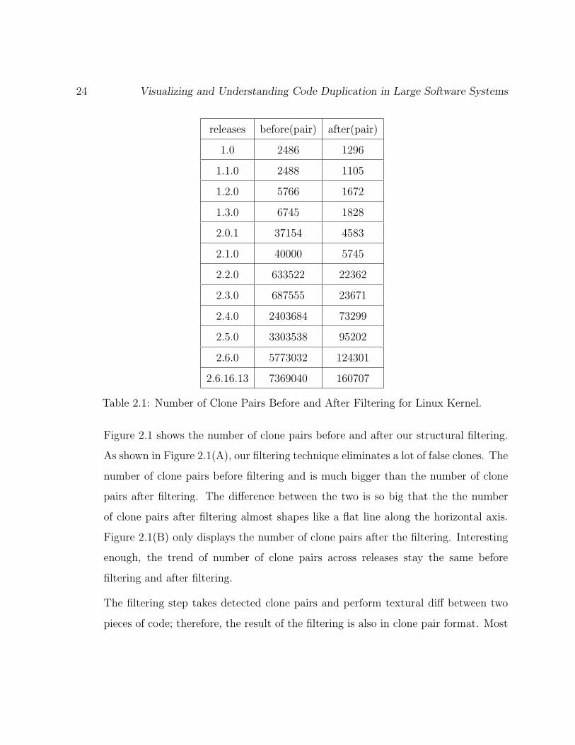
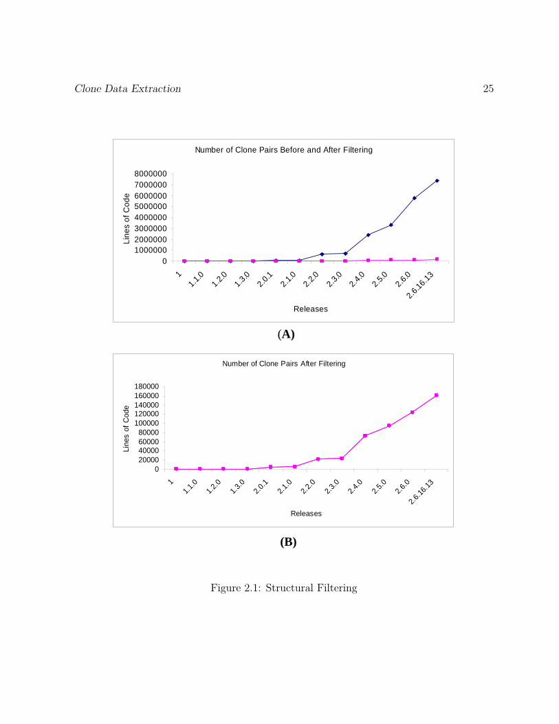
Table 2.1: Number of Clone Pairs Before and After Filtering for Linux Kernel.
Figure 2.1 shows the number of clone pairs before and after our structural filtering.
As shown in Figure 2.1(A), our filtering technique eliminates a lot of false clones. The
number of clone pairs before filtering and is much bigger than the number of clone
pairs after filtering. The difference between the two is so big that the the number
of clone pairs after filtering almost shapes like a flat line along the horizontal axis.
Figure 2.1(B) only displays the number of clone pairs after the filtering. Interesting
enough, the trend of number of clone pairs across releases stay the same before
filtering and after filtering.
The filtering step takes detected clone pairs and perform textural diff between two
pieces of code; therefore, the result of the filtering is also in clone pair format. Most
Clone Data Extraction 25
Number of Clone Pairs Before and After Filtering
010000002000000300000040000005000000600000070000008000000
11.1
.01.2
.01.3
.02.0.
12.1
.02.2
.02.3
.02.4
.02.5.
02.6
.0
2.6.16
.13
Releases
Line
s of
Cod
e
Number of Clone Pairs After Filtering
020000400006000080000
100000120000140000160000180000
11.1
.01.2
.01.3
.02.0
.12.1
.02.2
.02.3
.02.4
.02.5
.02.6
.0
2.6.16
.13
Releases
Line
s of
Cod
e
(A)
(B)
Figure 2.1: Structural Filtering
26 Visualizing and Understanding Code Duplication in Large Software Systems
of our study uses clone classes. We write a Perl script to transform the data format
from clone pairs to clone classes.
In summary, this chapter describes the steps to obtain cloning data in this thesis. The
data is initially extracted from a clone detection tool, CCFinder. Then textual filtering is
applied to remove the inappropriate clone relations.
Chapter 3
Related Work
In this chapter, we present two areas of related work: clone visualization and clone evolu-
tion.
3.1 Clone Visualization
For large software systems, clone detection tools usually report a large number (thousands)
of clone pairs and clone classes. In order to help software maintainers in examining the
output of clone detection tools, several clone visualization approaches and tools have be
proposed in literature.
We break down previous clone visualization approaches along two dimensions:
1. Visualized Source Entities: Are clones shown at the code segment level, lifted to
the file level, or lifted to the subsystem level? Higher abstractions (such as subsys-
tems) permit the study of large software systems since they reduce the amount of
clutter shown in the generated visualization.
27
28 Visualizing and Understanding Code Duplication in Large Software Systems
2. Visualized Clone Relations: Are clones shown as clone pairs, grouped as clone
classes, or grouped as super clone classes? By grouping clone code segments between
common files or subsystems, then practitioners can concentrate on suspicious (large
amounts of) cloning between two source entities instead of being overwhelmed by
many smaller clone pairs.
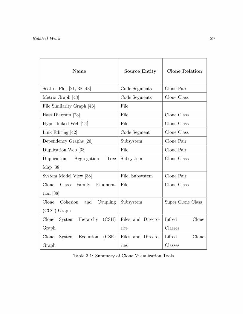
Table 3.1 summarizes current clone visualization research along these two dimensions.
The table also compares our presented visualizations to prior work. It categorizes each
visualization along two dimensions: the source entities the tool visualizes (such as code
segment level, file level or subsystem level) and the clone relations the tool visualizes (such
as clone pairs, clone classes or super clone classes).
In addition, our Clone Cohesion and Coupling (CCC) graphs visualize the cloning
relations by clone classes rather than clone pairs. Kapster et al. [26] show cloning relations
in boxes-and-arrows like architectural diagrams. They visualize cloning pairs between
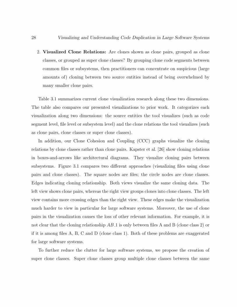
subsystems. Figure 3.1 compares two different approaches (visualizing files using clone
pairs and clone classes). The square nodes are files; the circle nodes are clone classes.
Edges indicating cloning relationship. Both views visualize the same cloning data. The
left view shows clone pairs, whereas the right view groups clones into clone classes. The left
view contains more crossing edges than the right view. These edges make the visualization
much harder to view in particular for large software systems. Moreover, the use of clone
pairs in the visualization causes the loss of other relevant information. For example, it is
not clear that the cloning relationship AB 1 is only between files A and B (clone class 2) or
if it is among files A, B, C and D (clone class 1). Both of these problems are exaggerated
for large software systems.
To further reduce the clutter for large software systems, we propose the creation of
super clone classes. Super clone classes group multiple clone classes between the same
Related Work 29
Name Source Entity Clone Relation
Scatter Plot [21, 38, 43] Code Segments Clone Pair
Metric Graph [43] Code Segments Clone Class
File Similarity Graph [43] File
Hass Diagram [23] File Clone Class
Hyper-linked Web [24] File Clone Class
Link Editing [42] Code Segment Clone Class
Dependency Graphs [26] Subsystem Clone Pair
Duplication Web [38] File Clone Pair
Duplication Aggregation Tree
Map [38]
Subsystem Clone Class
System Model View [38] File, Subsystem Clone Pair
Clone Class Family Enumera-
tion [38]
File Clone Class
Clone Cohesion and Coupling
(CCC) Graph
Subsystem Super Clone Class
Clone System Hierarchy (CSH)
Graph
Files and Directo-
ries
Lifted Clone
Classes
Clone System Evolution (CSE)
Graph
Files and Directo-
ries
Lifted Clone
Classes
Table 3.1: Summary of Clone Visualization Tools
30 Visualizing and Understanding Code Duplication in Large Software Systems
Clone Class 1
File A File B
File C File D
Clone Class 2
(B) Visualizing Cloning Relations With
Clone Classes
File A File B
File C File D
AB_1AB_2
AC BD
AD BC
CD
(A) Visualizing Cloning Relations With
Clone Pairs
Figure 3.1: Comparison between two approaches
source entities. These super clone classes aggregate many small clone classes into one
large super clone. These super clone classes help us deal with the limitation of simple
text comparison techniques and other clone techniques which may not recognize variation
points and may instead report them as separate clones. These super clone classes help
highlight and summarize to developers the magnitude of cloning between two source code
entities.
The Clone System Hierarchy (CSH) graph and the System Model View [38] display the
cloning information in a directory structure. They both use the node size and edge width
to indicate the amount of internal and external cloning. However, the System Model View
shows the cloning relations between files whereas CSH can display cloning relations for any
subsystems or files. In addition, CSH highlights the cloning relations by mouse movement
rather showing all the edges in the graph. Therefore, CSH has less cross-cutting edges and
contains more detailed cloning information than System Model View.
Related Work 31
No previous techniques, to the author’s knowledge, has been proposed to visualize
the evolution of code clones. Clone System Evolution(CSE) graph is the first attempt to
display the change of code cloning over time.
3.2 Clone Evolution
Lague et al. [4] studies the clone evolution on six subsequent versions of a large telecom-
munication projects over a period of three years. They incorporate the metric based clone
detection technique and found out that even though old clones have been removed and
but the overall number of clones keep increasing since new clones have been added in at a
faster pace. They classify clone changes as new clones, deleted clones and modified clones.
Merlo et al. [15] analyzes 365 releases(from 1994 to 2001) of Linux kernel are analyzed.
They uses the metric approach as their clone detection technique and found out that as
system evolves over time, the quality of the code base does not degenerate because of
cloning. As the addition of similar subsystem is accomplished through code reuse rather
than code cloning.
Kim et al. [27] proposed a clone genealogy extractor which tracks individual clone
instances over multiple releases. They present a more fine grained clone change patterns:
same, add, subtract, consistent change, inconsistent change and finally shift. Their case
study using the genealogy extractor shows that many clones are short lived and long lived
clones usually change consistently over time and are not easily refactorable.
In summary, this chapter cover the previous work related to this thesis, namely the
related work in the area of clone visualization and clone evolution.
Chapter 4
Clone Cohesion and Coupling (CCC)
Graph
This chapter introduces Clone Cohesion and Coupling (CCC) graph, which visualizes the
amount of internal cloning and external cloning for subsystems.
Coupling and cohesion between subsystems are commonly studied metrics when ana-
lyzing the architecture of large software systems. It is usually desirable for subsystems to
have high cohesion within the subsystem and to have low coupling to other subsystems.
In this chapter, we extend the ideas of coupling and cohesion to code cloning. As it has
been previously explained, a code clone is a segment of code that has been created through
duplication of another piece of code. Previous research has shown that in some instances
code cloning is desirable, whereas in other cases it is not. This thesis takes the position
that it is justifiable to have code cloning within subsystems (high cohesion), whereas it is
not justifiable and likely not desirable to have it across subsystems (high coupling).
We present an approach, which consists of a framework that generates cloning data and
a visualization technique for visualizing clone cohesion and coupling. Our approach can be
32
Clone Cohesion and Coupling (CCC) Graph 33
used by developers to locate undesirable cloning in their software system. We demonstrate
our approach through a case study on the code responsible for SCSI drivers in the Linux
kernel.
The rest of this chapter is organized as follows. Section 4.1 discusses the concept of
the architecture of clones as well as the concept of clone cohesion and clone coupling.
Section 4.2 presents our clone architecture recovery framework and discusses the data
schema used in our framework. We present our visualizations and showcase their main
benefits and features. Section 4.3 demonstrates our visualizations using a case study from
the Linux Kernel (in particular its SCSI drivers). Finally, section 4.4 shows a brief usage
guideline for researchers who are interested in using our visualization.
4.1 Architecture of Clones
Software architecture [17] provides a high-level understanding of large software systems. By
analogy, we introduce the concept of Architecture of Clones 1 in the hope of abstracting
a large volume of cloning information. The architecture of clones and software architecture
both consist of two parts: components and connectors. Table 4.1 compares these two kinds
of architectures. Components in both architectures refer to a collection of computation
units, referred as subsystems. Connectors in software architecture refer to the description
of interaction among components, such as data flow, call dependencies and so on, whereas
in the context of architecture of clones, they mean cloning relations.
The terms cohesion and coupling are commonly used in studying the design or archi-
tecture of a software system. These terms measure the structure of dependencies within
each subsystem and between subsystems (a subsystem contains files or other subsystems),
1We decide not to name it as “Clone Architecture” as to avoid the confusion of copying an architecture.
34 Visualizing and Understanding Code Duplication in Large Software Systems
Category Software Architecture Architecture of Clones
Components Subsystems Subsystems
Connectors Data/Dependency Cloning
Cohesion and Coupling Dependency Internal and External
Cloning
Examples Pipe and Filters, Client and
Server
Forking, Templating
Table 4.1: Comparison Between Software Architecture and Architecture of Clones
respectively. Coupling is concerned with dependencies between subsystems; while cohesion
refers to the dependencies within the subsystem. It is commonly desirable for a software
architecture to have low coupling and high cohesion. For example, a subsystem with a
large number of functions that are dependant on each other (high cohesion) is more desir-
able than a subsystem where functions depend heavily on functions in other subsystems
(high coupling). This intuition forms the basis of many modern software clustering tech-
niques [33].
Highly cohesive subsystems are desirable since they imply that subsystems represent
closely related concerns. Low coupling is also desirable since it implies that the subsystems
are relatively easy to modify and evolve. Developers changing software systems with low
coupling can have their changes focused to a limited number of subsystems instead of
needing to propagate their changes to a large number of subsystems.
In this thesis, we extend the concepts of coupling and cohesion to code cloning. This
thesis takes the position that it is justifiable to have some cloning within a subsystem (clone
cohesion); whereas it is not desirable to have cloning across subsystems (clone coupling).
Cloning within a subsystem is “justifiable” since it is likely due to the similarity between

Clone Cohesion and Coupling (CCC) Graph 35
functions and files within a subsystem. Large amount of cloning across subsystems is not
“justifiable” since it is expected that subsystems represent different concerns that are not
similar and therefore should not share a large amount of code cloning. This intuition is
analogous to coupling for code dependencies, where it is not desirable to have coupling
between different subsystems. In summary, we consider that low code coupling and high
code cohesion are desirable, and low clone coupling and high clone cohesion are justifiable.
We use the term justifiable for clone coupling and cohesion since as we mentioned earlier
that may be good reasons to clone code and there are no definitive research results that rule
out the shortcomings or advocate the benefits of clones [27]. Determining whether a clone
is desired or not should be done on a project by project basis by system experts. In this
chapter, we present an approach to assist system experts to study cloning in their software
system. The approach presents a visualization that a system expert use to gain an overview
of the amount of clone cohesion and coupling in their software system. Using the same
visualization, the system expert can investigate specific code clones to determine if they
are justifiable or not. If they are not justifiable, then the system expert can schedule their
removal as part of future code refactoring activities. The visualization as well permits
the system expert to perform “What-if” analysis to determine the impact of removing
particular clones and to determine the amount of effort needed to remove clones between
subsystems in large software systems.
4.2 Our Approach
The main motivation for our visualization is to assist practitioners in coping with the large
amount of results displayed by clone detection tools. The main purpose of the generated
visualization is to highlight to developers cloning within each subsystem and across sub-
36 Visualizing and Understanding Code Duplication in Large Software Systems
systems. Developers can then investigate whether the cloning is undesirable or not. For
example, if a developer examining our visualization notices that there is a large amount
of cloning between the memory manager and the network drivers in Linux, then he or she
may be alarmed since there is no clear justifiable reason for such cloning to occur. On the
other hand if our visualization highlighted that two similar driver families using the same
hardware chipset have a large amount of common code then the developer may consider
such cloning justifiable. The developer may later consult other senior developers to de-
termine whether such cloning is desirable. In short, our produced visualization highlights
potentially troublesome clones and we permit developers to study them closely instead of
displaying all clones between all code segments in large software systems.
We now detail the main two components of our approach: a clone recovery framework
and clone visualization.
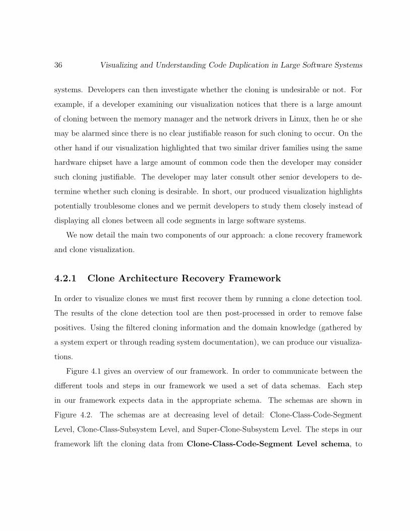
4.2.1 Clone Architecture Recovery Framework
In order to visualize clones we must first recover them by running a clone detection tool.
The results of the clone detection tool are then post-processed in order to remove false
positives. Using the filtered cloning information and the domain knowledge (gathered by
a system expert or through reading system documentation), we can produce our visualiza-
tions.
Figure 4.1 gives an overview of our framework. In order to communicate between the
different tools and steps in our framework we used a set of data schemas. Each step
in our framework expects data in the appropriate schema. The schemas are shown in
Figure 4.2. The schemas are at decreasing level of detail: Clone-Class-Code-Segment
Level, Clone-Class-Subsystem Level, and Super-Clone-Subsystem Level. The steps in our
framework lift the cloning data from Clone-Class-Code-Segment Level schema, to
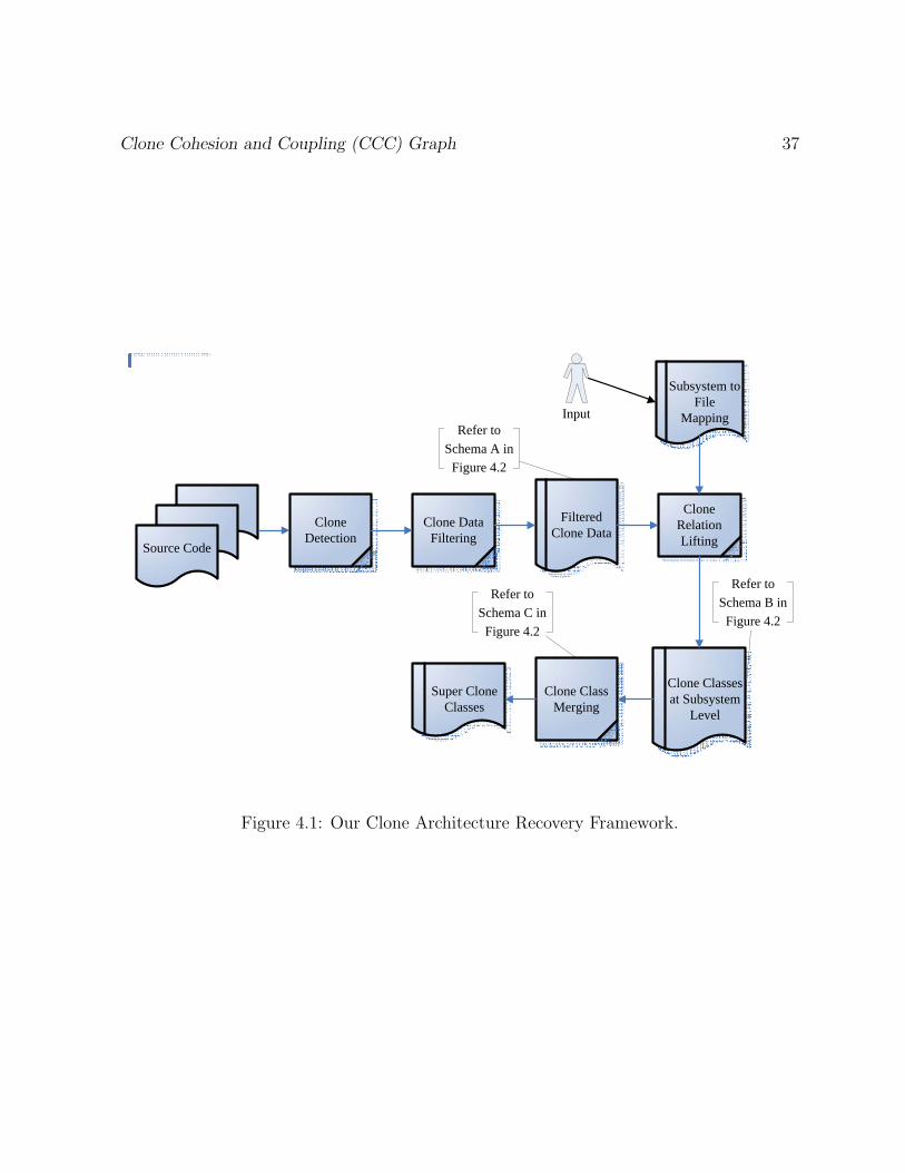
Clone Cohesion and Coupling (CCC) Graph 37
Clone Detection
Clone Data Filtering
Filtered Clone Data
Source Code
Clone Relation Lifting
Subsystem to File
Mapping
Clone Classes at Subsystem
Level
Clone Class Merging
Super Clone Classes
InputRefer to
Schema A in Figure 4.2
Refer to Schema B in
Figure 4.2
Refer toSchema C in
Figure 4.2
Figure 4.1: Our Clone Architecture Recovery Framework.
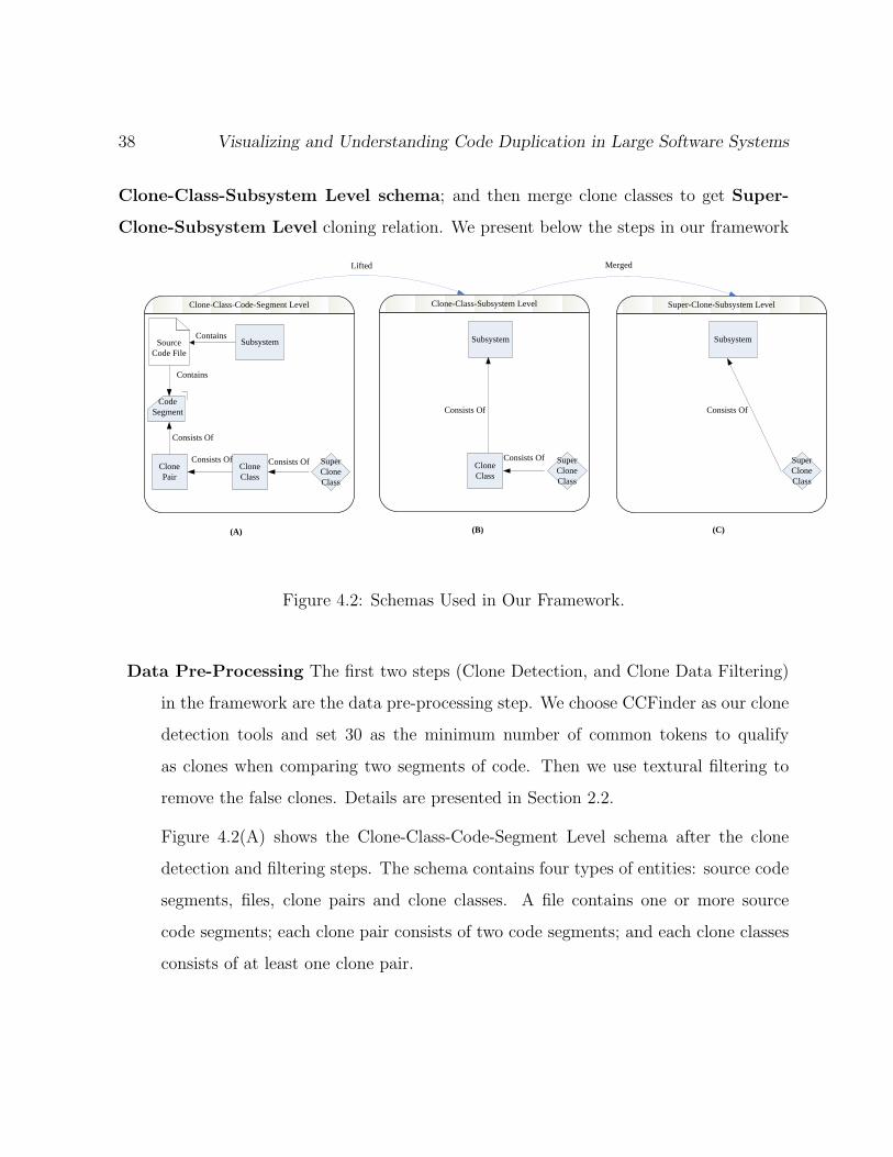
38 Visualizing and Understanding Code Duplication in Large Software Systems
Clone-Class-Subsystem Level schema; and then merge clone classes to get Super-
Clone-Subsystem Level cloning relation. We present below the steps in our framework
Source Code File
Code Segment
Clone Class
Clone-Class-Code-Segment Level
Clone Pair
Consists Of Clone Class
Clone-Class-Subsystem Level Super-Clone-Subsystem Level
(A) (B) (C)
Lifted Merged
Consists Of
Consists Of
Contains
Consists Of
Consists Of Consists Of
ContainsSubsystem Subsystem Subsystem
Super CloneClass
Super CloneClass
Super CloneClass
Figure 4.2: Schemas Used in Our Framework.
Data Pre-Processing The first two steps (Clone Detection, and Clone Data Filtering)
in the framework are the data pre-processing step. We choose CCFinder as our clone
detection tools and set 30 as the minimum number of common tokens to qualify
as clones when comparing two segments of code. Then we use textural filtering to
remove the false clones. Details are presented in Section 2.2.
Figure 4.2(A) shows the Clone-Class-Code-Segment Level schema after the clone
detection and filtering steps. The schema contains four types of entities: source code
segments, files, clone pairs and clone classes. A file contains one or more source
code segments; each clone pair consists of two code segments; and each clone classes
consists of at least one clone pair.
Clone Cohesion and Coupling (CCC) Graph 39
Clone Relation Lifting At this stage, each clone class contains a set of code segments
from different files. We use two lifting operations here. First, we lift information
to the file level (i.e. we lift our cloning data from Clone-Class-Code-Segment level
to Clone-Class-File level). For example, if clone class A contains lines 110 − 130 in
file1.c, lines 210 − 230 in file2.c and lines 10 − 30 in file3.c, then the lifting will
results in clone class A containing 20 lines of cloned code, which reside in files file1.c,
file2.c, and file3.c, respectively.
Since we plan to visualize relations between subsystems, we need to lift our cloning
data to the Super-Clone-Class-Subsystem level. Several clone classes might contain
the same set of subsystems or some of them might only contain one subsystem as all
the duplicates are within the same subsystems.
To perform the lifting to the subsystem level, we need a mapping from files to sub-
systems. Ideally, such a mapping would be provided by a system expert. However,
if we don’t have an expert, as suggested in [6], we have to create this mapping by
a few heuristics: such as consulting the documentation, grouping files based on di-
rectory structure and naming conventions or manually examining the source code.
Continuing the above example, if file1.c is in subsystem S1, file2.c in subsystem S2,
and file3.c in subsystem S3; then the lifting result will create clone class A which
contains consists of subsystems S1, S2 and S3 which contain 20 duplicated lines,
respectively.
Note that, subsystems can contain smaller subsystems. Therefore, depending on the
level of system abstractions desired, repeated lifting process should be performed,
accordingly. Figure 4.2(B) shows the Clone-Class-Subsystem Level schema after the
lifting step. The data at this level contains two types of entities: clone classes and
subsystems. Each clone classes consists of at least one subsystem.
40 Visualizing and Understanding Code Duplication in Large Software Systems
Merging of Clone Classes
In this final step, we aggregate the clone classes which contain the same set of subsys-
tem(s) to simplify the cloning relationship. For example, suppose clone classes 128
and 233 both contains subsystems S1, S2 and S3 and no more. We can merge these
two clone classes into one super clone class node. Super clone class nodes are named
after the names of the subsystems in which the super clone classes contain. If they
cross multiple subsystems, then each subsystem is separated by a “#” sign. In the
above example, the super clone class is named as S1#S2#S3 to indicate that they
all exactly contain subsystems S1, S2 and S3. We found that this naming convention
helps easily identify the degree of cloning in a super clone in our visualization instead
of having users follow a large number of edges.
Figure 4.2(C) shows the Super-Clone-Class-Subsystem schema. There are two types
of entities here: Super Clone Classes and subsystems. Each super clone class contains
one or more subsystems.
4.2.2 Clone Cohesion and Coupling (CCC) Graph
The main goal of our Clone Cohesion and Coupling (CCC) graph visualization is to high-
light cloning within each subsystem (cohesion) and across subsystems (coupling). To help
to direct practitioners to the most troublesome spots, we define “cloning hotspots” that
are brightly colored large nodes that would capture the attention of the viewer.
A secondary goal of our visualization is to show how different subsystems are interre-
lated according to cloning. Our cloning visualization shows close together subsystems that
have a large amount of common code due to cloning, and shows far apart subsystems that
have little cloning between each other.
Clone Cohesion and Coupling (CCC) Graph 41
We now discuss the different entities in our visualization. See Figure 4.4 for an example
of this visualization. The graph consists of two types of entities: nodes and edges. There are
two types of nodes in our graphs: rectangle nodes (subsystems) and diamond nodes (super
clones). An edge between a rectangle and a diamond represents a cloning relationship.
We now explain the semantics of our visualization by showing how we satisfy our
aforementioned goals.
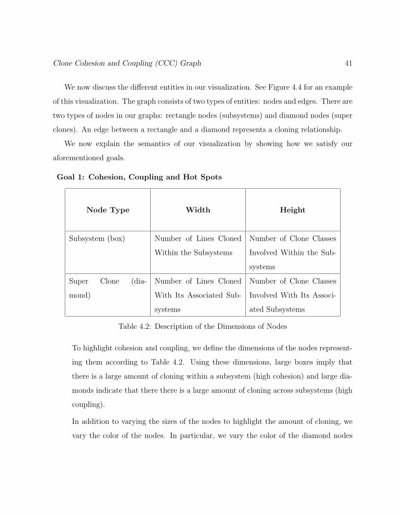
Goal 1: Cohesion, Coupling and Hot Spots
Node Type Width Height
Subsystem (box) Number of Lines Cloned
Within the Subsystems
Number of Clone Classes
Involved Within the Sub-
systems
Super Clone (dia-
mond)
Number of Lines Cloned
With Its Associated Sub-
systems
Number of Clone Classes
Involved With Its Associ-
ated Subsystems
Table 4.2: Description of the Dimensions of Nodes
To highlight cohesion and coupling, we define the dimensions of the nodes represent-
ing them according to Table 4.2. Using these dimensions, large boxes imply that
there is a large amount of cloning within a subsystem (high cohesion) and large dia-
monds indicate that there there is a large amount of cloning across subsystems (high
coupling).
In addition to varying the sizes of the nodes to highlight the amount of cloning, we
vary the color of the nodes. In particular, we vary the color of the diamond nodes

42 Visualizing and Understanding Code Duplication in Large Software Systems
Figure 4.3: Heat Coloring.
since we believe that cross subsystem coupling (i.e. high coupling) is troublesome
and should be investigated. We consider large diamonds as “cloning hot-spots”. We
“heat color” super clones using a quartile based coloring technique. The color of a
diamond is based on the total number of lines cloned across subsystems in that super
clone node. We choose the total lines of cloned code rather than the total number of
cross family clones since we feel that total lines of cloned code is a better indicator
of how much effort will be required to examine and refactor a particular super clone
node.
The “Heat Coloring” works by calculating the median and the quartiles (the lower
quartile is the 25th percentile and the upper quartile is the 75th percentile), the value
range of the studied metric is divided into four quarters, which are associated with
four different colors respectively. In our case studies, we have chosen red, yellow,
light-green, and light-grey as shown in Figure 4.3.
Goal 2: Overall System Cloning View
In order to demonstrate the interrelations between different subsystems according to
cloning, we apply a force-based graph layout [41] in our visualization to arrange the
Clone Cohesion and Coupling (CCC) Graph 43
relative position of subsystems. Weights have been exerted to the edges to represent
the number of cloned lines from the subsystems to the super clone nodes. Subsystems
which have more duplications with each other will be placed closer to the super
clone classes; conversely, subsystems which have less cross-family cloning will be
pushed further away from the super clone nodes. Overall, subsystems which have a
large amount of code cloning with other subsystems will be placed closer to these
subsystems than other subsystems.
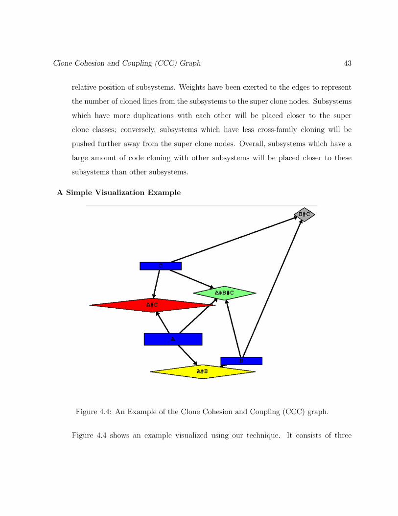
A Simple Visualization Example
Figure 4.4: An Example of the Clone Cohesion and Coupling (CCC) graph.
Figure 4.4 shows an example visualized using our technique. It consists of three
44 Visualizing and Understanding Code Duplication in Large Software Systems
subsystems: A, B, and C; and four super clone nodes: A#B#C, A#B, B#C, and
A#C. As indicated by the color: A#C has the biggest cross-subsystem cloning, sub-
systems A and C are pulled towards that super clone. The second largest super clone
node is A#B, followed by A#B#C, and finally B#C. Since B#C is the smallest
clones, subsystems B and C are pushed away from that super clone node. Subsystem
A is taller and wider, since it contains more internal cloning than other subsystems.
All super clone nodes are colored using the heat based coloring techniques.
4.3 Case Study: The Clone Architecture of SCSI Sub-
system
To demonstrate our framework, we present a study of cloning in the code responsible for
SCSI drivers in the Linux kernel. SCSI stands for “Small Computer System Interface”.
We believe studying SCSI drivers is a good case study to demonstrate clone cohesion and
coupling.
Device drivers are programs for interacting with hardware devices. Studies show that
writing device drivers is error-prone and is considered as a major source of errors in oper-
ating systems [10]. Around 30% of the source code files in the Linux Kernel are devoted
for implementing various device drivers. Due to the similarity between hardware devices
in the same family (i.e. from the same vendor or that use the same hardware chipset),
developers are more likely to clone code between drivers in the same family in order to
speed up development and reduce the likelihood of errors. Therefore, we believe that it
is justifiable and probably desirable to have cloning within a driver family. However, it
may not be justifiable nor desirable to have cloning across different driver families; since
drivers from different families resemble little similarities thus these types of cloning might
Clone Cohesion and Coupling (CCC) Graph 45
be questionable. Developers have to be aware of such cross family cloning and may need to
propagate changes across driver families. Such change propagation are likely to introduce
errors over time as developer forget such unexpected dependencies.
4.3.1 Results of Our Clone Extraction Framework
All code in the SCSI related directories in Linux consists of 858, 727 tokens, 476, 612 lines,
and 381 files. CCFinder (with 30 tokens as the minimum clone size) reported that this
code has 54, 195 clone pairs and 2, 034 clone classes. After filtering the non-function clones,
we have 305 clone classes left. We have 119 clone classes which cross cut two or more
subsystems. We have obtained 33 super clone nodes after the merging process, about 67%
of them cross cut two or three subsystems.
4.3.2 Subsystem Mapping
An important input needed for our framework is the mappings from files to subsystems.
Ideally, a system expert would provide such a mapping. Unfortunately, we don’t have
one. By reading documentation, analyzing source code and examining files, we created a
subsystem mapping. Our subsystem mapping groups files belonging to the same driver
family (similar vendor or similar driver chip in the same family) in the same subsystem.
We now explain how we built our mapping.
There are 425 files that are in the directories that implement the SCSI drivers in the
Linux Kernel version 2.6.16.13. Nevertheless, many of these files do not implement drivers
but rather they are testing or libraries files. For our study we decided to only focus on
files that implement specific SCSI drivers. To uncover such files, we started by parsing the
Makefiles responsible for building the SCSI drivers in the Linux Kernel. We show below
an excerpt of a Makefile for SCSI.
46 Visualizing and Understanding Code Duplication in Large Software Systems
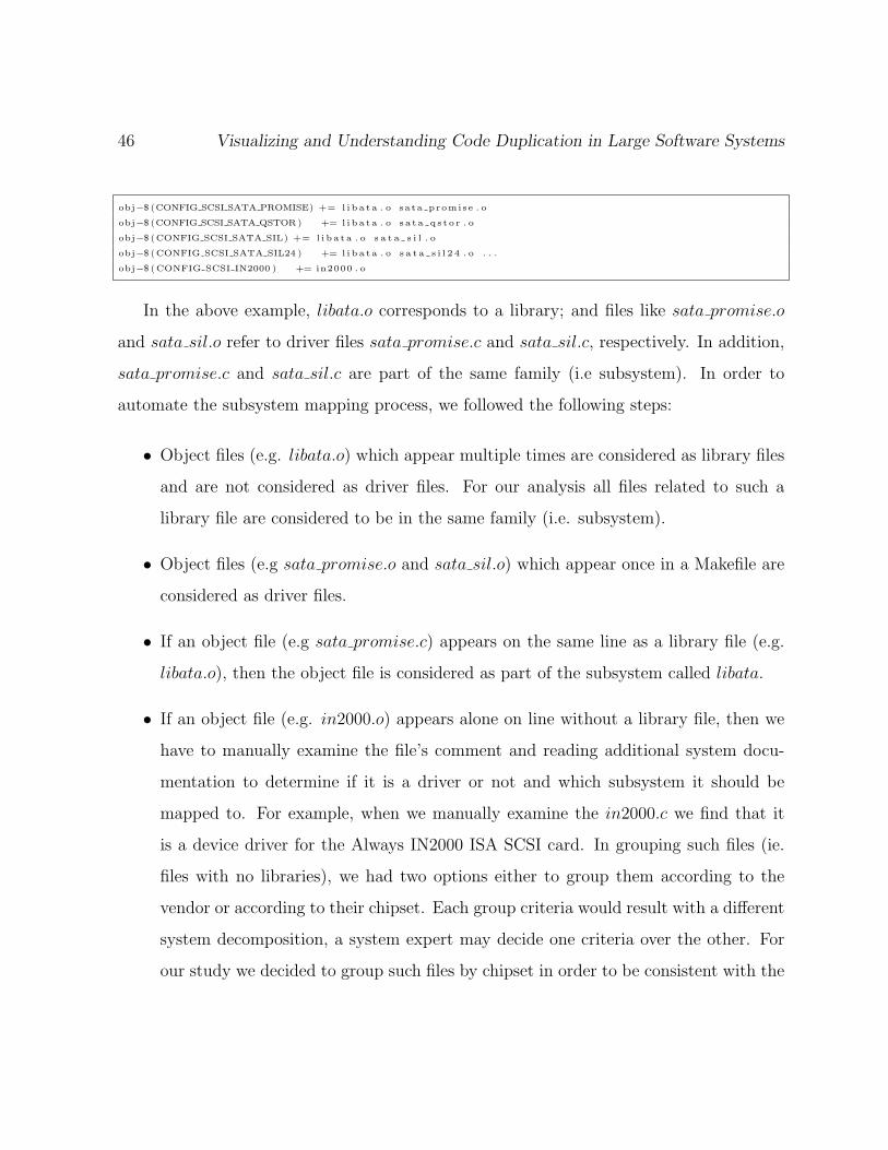
obj−$ (CONFIG SCSI SATA PROMISE) += l i b a t a . o sata promise . o
obj−$ (CONFIG SCSI SATA QSTOR) += l i b a t a . o s a t a q s t o r . o
obj−$ (CONFIG SCSI SATA SIL) += l i b a t a . o s a t a s i l . o
obj−$ (CONFIG SCSI SATA SIL24 ) += l i b a t a . o s a t a s i l 2 4 . o . . .
obj−$ (CONFIG SCSI IN2000 ) += in2000 . o
In the above example, libata.o corresponds to a library; and files like sata promise.o
and sata sil.o refer to driver files sata promise.c and sata sil.c, respectively. In addition,
sata promise.c and sata sil.c are part of the same family (i.e subsystem). In order to
automate the subsystem mapping process, we followed the following steps:
• Object files (e.g. libata.o) which appear multiple times are considered as library files
and are not considered as driver files. For our analysis all files related to such a
library file are considered to be in the same family (i.e. subsystem).
• Object files (e.g sata promise.o and sata sil.o) which appear once in a Makefile are
considered as driver files.
• If an object file (e.g sata promise.c) appears on the same line as a library file (e.g.
libata.o), then the object file is considered as part of the subsystem called libata.
• If an object file (e.g. in2000.o) appears alone on line without a library file, then we
have to manually examine the file’s comment and reading additional system docu-
mentation to determine if it is a driver or not and which subsystem it should be
mapped to. For example, when we manually examine the in2000.c we find that it
is a device driver for the Always IN2000 ISA SCSI card. In grouping such files (ie.
files with no libraries), we had two options either to group them according to the
vendor or according to their chipset. Each group criteria would result with a different
system decomposition, a system expert may decide one criteria over the other. For
our study we decided to group such files by chipset in order to be consistent with the

Clone Cohesion and Coupling (CCC) Graph 47
grouping created by the Makefile. The grouping obtained from the Makefile, in the
previous steps, is based on the chipset.
This process has helped us identify 109 drivers and we created 17 driver subsystems
(i.e. families). Our automatic Makefile clustering has helped us cluster 56 drivers. The
remaining drivers are clustered manually.
4.3.3 Clone Cohesion and Coupling (CCC) Graph
Figure 4.5 shows a screenshot of our Clone Cohesion and Coupling graph for the SCSI
driver subsystems. The figure shows a zoomed out view of the visualization. On the right
side of the figure we mark a few noteworthy nodes. The figure is generated using the aiSee
tool [1] which permits us to zoom in and zoom out the diagram. The forced-based graph
layout permits us to see the degree of clone coupling between subsystems. For example,
IOMEGA and FUTUREDOMAIN are more tightly coupled than ATA and NCR53C9x.
In our study we focus on the hot spots (large red diamond nodes and large boxes). Our
visualization indicates that there is a large amount of cloning within the ATA and IOMEGA
subsystems (i.e. both subsystems have high clone cohesion). We also investigated two of
the largest diamond nodes since they indicate high coupling between subsystems).
ADAPTEC#IOMEGA is one of the biggest super clone nodes (Number 5 in Fig-
ure 4.5). It contains 864 lines of cloned code and has 5 driver files across two subsystems
(ADAPTEC and IOEMA). By manually examining source code, we discover that this
super clone node is superfluous. The clones are code segments that contain case switch
statements. It is a false clone produced by CCFinder. CCFinder tokenizes the source code
and recognizes the similar code structures.
ULTRASTOR#EATA is another big super clone node (Number 1 in Figure 4.5). A
closer analysis of this super clone node reveals that it contains 14 clone classes and all the

48 Visualizing and Understanding Code Duplication in Large Software Systems
Super Clones: 1. ULTRASTOR#EATA 2. ULTRASTOR#EATA#RAID 3. ADAPTEC#NCR580 4. ADAPTEC#NCR580#TEKRAM 5. ADAPTEC#IOMEGA
Subsystems (Driver Family): 6. ATA 7. NCR53C9x 8. NCR5380 9. FUTUREDOMAIN 10. IOMEGA
12
3
45
6
7
9
10
8
Figure 4.5: Annotated Screenshots of the CCC graph for the Linux SCSI drivers.
Clone Cohesion and Coupling (CCC) Graph 49
cloning occurs between only two files: eata.c from the EATA family and u14−34f.c from the
ULTRASTOR family. They are neither from the same vendor nor do they have a common
hardware chipset. eata.c is the Low-level driver for EATA/DMA SCSI host adapters and
u14− 34f.c is the Low-level driver for UltraStor 14F/34F SCSI host adapters. We decided
to explore the reason behind such large degree of coupling between both subsystems (in
particular both files). We manually inspected the change logs for both files. The change
logs indicate that changes to both files are almost identical and that changes occur almost
at the same date throughout the lifetime of both files. Moreover, we discovered that
the copyright for both files is attributed to the same person. We suspect that the same
developer has cloned one of the files as part of knowledge transfer from one driver to the
other. As development progresses, the clones have been maintained synchronously.
The visualization has been able to highlight the most noteworthy clones across subsys-
tems and within subsystems. Using the visualization we are able to quickly locate these
noteworthy and investigate them instead of investigating a large number of clone pairs in
an ad-hoc manner.
4.4 Usage Guideline
We summarize the steps for using our visualization. Researchers can follow this guidelines
to process, visualize and analyze cloning for other software systems.
Overall Process: Take the above case study for example. Inside Linux scsi subsys-
tem, cloning can occur among drivers which share same hardware platform, or from
the same manufacture, etc. Therefore, there can be different criteria to group files
into subsystems. So, it is recommended to produce several CCC graphs using dif-
ferent subsystem decomposition and cross-examine the interesting spot. A thorough
50 Visualizing and Understanding Code Duplication in Large Software Systems
empirical clone study on SCSI drivers should examine the subsystem level cloning
according to different subsystem decomposition. For example, driver files can be
grouped by parsing the Makefiles (check Section 4.3.2) or by file name similarity
(such as “sun3 NCR5380.c” and “atari NCR5380.c” are similar) or by the length of
file sizes (files with similar sizes are grouped together), etc.
Using each subsystem grouping, a CCC graph is generated and analyzed. The aim is
to investigate places where it has heavy cloning. For example, we need to investigate
subsystems which have heavy internal cloning to see whether it is justifiable as well
as examining big super clones to see whether it is desirable.
Data Processing: Lifting refers to the process of aggregating the cloning data from
the file level to the subsystem level. Lifting process is repeated until it reaches to the
level of system abstractions desired. The lifting process can be stopped at the lowest
subsystem level or be performed all the way up to the top level subsystems or to any
intermediate levels in between.
Once lifting is done, merging combines the clone classes into one bigger clone classes.
Note that, merging is invoked only if clone classes contains exactly the same set of
subsystems.
Graph Analysis: We now describe a few issues that require attention for:
Thin Rectangle Nodes are subsystems that contain a lot of duplicated code
segments but each clone is relatively small. This type of nodes is worth inves-
tigating since it could possibly be a cross-cutting concern or just repeated code
idioms.
Flat Rectangle Nodes are subsystems that contains very few cloned segments
Clone Cohesion and Coupling (CCC) Graph 51
but a lot of code gets duplicated. This could possibly be a copy of entire source
code file.
Red Diamond Nodes are a group of clone classes which have the largest number
of cross-subsystem cloning. We need to further investigate why these subsystems
are tightly coupled.
Diamond Nodes with Several “#”: we name the merged clone class as the
names of the clone classes to be merged separated by “#”s. For example, if we
merge clone class 1 and 2, the super clone class is 1#2. If a super clone class
has several “#”s, this means that clones are cross-cut across many subsystems.
We need to further investigate the reason behind this cloning. Is it due to our
system decomposition, these files should be grouped into one subsystem? Or is
it a coding idiom? Or is it something else?
In addition, researchers need to consult other references, such as documentation, the
source code itself, static dependencies, etc., to uncover the original rationale behind cloning.
4.5 Conclusion
The chapter proposes Clone Cohesion and Coupling (CCC) graph, which visualizes code
cloning at the subsystem level. The graph shows the amount of internal cloning and
external cloning in each subsystem. In particular, the force-based graph layout and heat
colouring of the super clone class nodes highlights the surprising cloning relations among
subsystems.
Chapter 5
Clone System Hierarchical(CSH)
Graph
In this chapter we propose Clone System Hierarchical (CSH) graph, which visualizes
cloning data in a directory tree.
The goal of this thesis is to develop tools and techniques to assist researcher to better
analyze code cloning in large software systems. A major obstacle researchers face is how
to handle large volume of cloning data. Chapter 4 presents Clone Cohesion and Cou-
pling(CCC) Graph, which displays the cloning information at subsystem level. It provides
users with an overview of the amount of internal and external cloning of the subsystems.
Unfortunately, the CCC graph lacks of cloning details; as it only displays cloning informa-
tion for one level of subsystems. It is unclear whether heavy cloning between two subsystem
is due to a small number of files or a large number of files. We need a visualization tool
which shows the details of the code duplication and preferably highlights the spread of the
cloning.
Knowing the spread of cloning at the file level is important because the more spread
52
Clone System Hierarchical (CSH) Graph 53
clones are, the more effort is required to modify the code base such as propagating bug
fixes selectively to clone instances or to perform re-engineering tasks such as refactoring
common code to eliminate clones. For example, “drivers/net/3c501.c” in Linux Kernel
version 1.0 has 11 files that have cloning relationships. It is relatively harder to maintain
than “drivers/FPU-emu/reg add sub.c”, which has code duplications with only 1 file.
Knowing the spread of cloning at the subsystem level is useful, since it helps to have a
deeper understanding of the design of the systems because it can uncover certain functional
relations or cloning patterns which are usually not documented. If we examine the cloning
of file system (fs) inside Linux Kernel, subsystems like “fs/ext2”, “fs/minix” have a lot
of external cloning with each other but little internal cloning. This is a sign of potential
“forking” pattern [11].
This chapter introduces Clone System Hierarchical (CSH) Graph which embeds the
cloning information in the directory tree. Although the cloning information can be em-
bedded into other backbone structures like subsystem decompositions, we feel directory-
structure tree is the most suitable framework for several reasons. Our visualization is used
to study the cloning phenomenon and developers are more comfortable working with di-
rectories. They navigate through directories and copy-paste code between files. Therefore,
it is more natural to conduct the cloning study within the directory trees. Our CSH graph
provides the details of copying at different levels of system abstractions. Researchers can
easily spot the amount of internal cloning and external cloning for each file and subsys-
tem. In addition, the CSH graph highlights the cloning relation for individual files and
subsystems, through mouse pointing and clicking.
The rest of this chapter is organized as follows: Section 5.1 explains the steps to lift
the cloning data to the system hierarchical level. Section 5.2 presents the Clone System
Hierarchy (CSH) graph. Section 5.3 provides some discussions with our visualization and

54 Visualizing and Understanding Code Duplication in Large Software Systems
presents some future work. Finally, Section 5.4 presents a short guideline for researchers
who are interested in using our visualization.
5.1 Clone System Hierarchy Extraction Framework
Before we can visualize cloning relationship at the subsystem level, we need to abstract
cloning data to the system level. Figure 5.1 illustrates the process. In order to communicate
among different tools and steps in our framework, we use a set of data schemas. Each step
in our framework expects data in the appropriate schema. The schemas are shown in
Figure 5.2. The schemas are at two level of abstractions: Clone-Class-Code-Segment Level
and Clone-Class-File-Subsystem Level. Our framework first lifts the cloning data from
Clone-Class-Code-Segment Level schema, and aggregates the cloning information
from lower subsystems to Clone-Class-Subsystem Level schema. We present below
the different steps in our framework.
Data Pre-Processing
Similar as the Clone Recovery Framework described in Section 4.2.1, the first two steps
in the framework are the data pre-processing step. We choose CCFinder as our clone
detection tools and set 30 as the minimum number of common tokens to qualify as clones
when comparing two segments of code. Then we use textural filtering to remove false
clones. Details are presented in Section 4.2.1
Figure 5.2(A) shows the Clone-Class-Code-Segment Level schema after the clone de-
tection and filtering steps. The data contains four types of entities: source code segments,
files, clone pairs and clone classes. A file contains one or more source code segments; each
clone pair consists of two code segments; and each clone classes consists of at least one
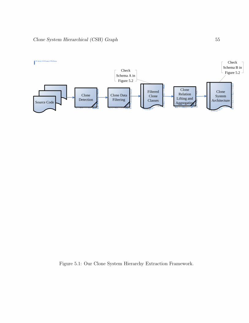
Clone System Hierarchical (CSH) Graph 55
Clone Detection
Clone Data Filtering
Filtered Clone
ClassesSource Code
Clone Relation
Lifting and Aggregating
Clone System
Architecture
Check Schema A in
Figure 5.2
Check Schema B in
Figure 5.2
Figure 5.1: Our Clone System Hierarchy Extraction Framework.

56 Visualizing and Understanding Code Duplication in Large Software Systems
Source Code File
Code Segment
Clone Class
Clone-Class-Code-Segment Level
Clone Pair
Clone Class
Clone-Class-Subsystem Level
(A)Clone Data
Lifted
Consists Of
Consists Of
Contains
Consists Of
ContainsSubsystem
(B)Lifted Clone Data
Subsystem
Contains Contains
Figure 5.2: Schemas Used in Our Framework.
Clone System Hierarchical (CSH) Graph 57
clone pair.
Clone Relation Lifting and Aggregating
Now each clone class contains cloning relations among code segments from different files.
The lifting operation is also the same as the lifting processes in Section 4.2.1. We first
lift the cloning information from code segment level to file level, the from file level to
lower level subsystem level, followed by lifting from lower level subsystem level to higher
subsystem level until all the way up to the top level subsystems. The only difference is
that, in Clone Recovery Framework the information before lifting is discarded whereas the
cloning information from the lower level entities (files, subsystems) are preserved. (In this
and the following chapters, we consider directory structure as the software architecture
decomposition. We use the term directory and subsystem interchangeably. Note that, for
other software architecture decompositions, we can use similar technique to lift the cloning
data and visualize it in the graph.) This processed in illustrated an an example shown in
Figures 1.6 and 1.7.
5.2 Clone System Hierarchical (CSH) Graph
The main goal of our visualization is to show the spread of cloning at different levels of
granularity: from top level directories to the lower level directories and lastly to the file
level.
As shown in Figure 5.3, our tool consists of 4 components: Node Name, Clone System
Hierarchical Tree, Selection Menu, and Clone Information Panel. Node Name shows the
name of the node currently examining. Clone System Hierarchical Tree is an interactive
graph that allows the user to point and click nodes to highlight the spread out of the
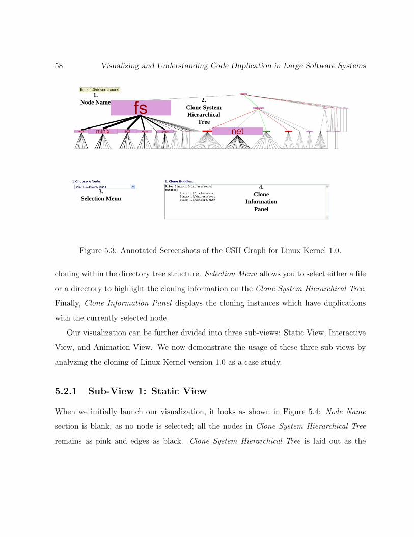
58 Visualizing and Understanding Code Duplication in Large Software Systems
1. Node Name 2.
Clone System Hierarchical
Tree
3.Selection Menu
4.Clone
Information Panel
Figure 5.3: Annotated Screenshots of the CSH Graph for Linux Kernel 1.0.
cloning within the directory tree structure. Selection Menu allows you to select either a file
or a directory to highlight the cloning information on the Clone System Hierarchical Tree.
Finally, Clone Information Panel displays the cloning instances which have duplications
with the currently selected node.
Our visualization can be further divided into three sub-views: Static View, Interactive
View, and Animation View. We now demonstrate the usage of these three sub-views by
analyzing the cloning of Linux Kernel version 1.0 as a case study.
5.2.1 Sub-View 1: Static View
When we initially launch our visualization, it looks as shown in Figure 5.4: Node Name
section is blank, as no node is selected; all the nodes in Clone System Hierarchical Tree
remains as pink and edges as black. Clone System Hierarchical Tree is laid out as the
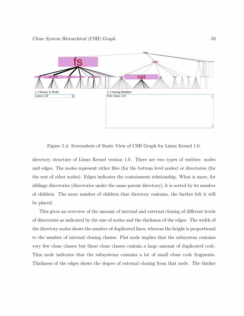
Clone System Hierarchical (CSH) Graph 59
1. Choose A Node:Linux-1.0/
2. Cloning BuddiesFile: linux-1.0/
Figure 5.4: Screenshots of Static View of CSH Graph for Linux Kernel 1.0.
directory structure of Linux Kernel version 1.0. There are two types of entities: nodes
and edges. The nodes represent either files (for the bottom level nodes) or directories (for
the rest of other nodes). Edges indicates the containment relationship. What is more, for
siblings directories (directories under the same parent directory), it is sorted by its number
of children. The more number of children that directory contains, the farther left it will
be placed.
This gives an overview of the amount of internal and external cloning of different levels
of directories as indicated by the size of nodes and the thickness of the edges. The width of
the directory nodes shows the number of duplicated lines; whereas the height is proportional
to the number of internal cloning classes. Flat node implies that the subsystem contains
very few clone classes but these clone classes contain a large amount of duplicated code.
Thin node indicates that the subsystems contains a lot of small clone code fragments.
Thickness of the edges shows the degree of external cloning from that node. The thicker
60 Visualizing and Understanding Code Duplication in Large Software Systems
the edges, the larger the amount of external cloning from that node. At the top level
directory, as implied from the size of the nodes: “fs” has more internal cloning than
“drivers” and “net”. Within “fs”, directories like “ext2”, “minix2”, “ext”, “xiafs”, and
“sysv” have a lot of external cloning as indicated by the thickness of the edges. We decide
to use the same size for the file nodes mainly for scalability concerns: if we embedded the
cloning information into the dimension of the file nodes it would be too big to fit them in
the screen; as there are too many files.
In addition, the CSH graph also provides us with a rough idea of the degree of code du-
plication within each directory. For example, “drivers/scsi”(the SCSI device drivers) is the
left-most directory among directories within “drivers”(all the device drivers). This implies
that “scsi” contains the largest number of files among its siblings directories. However,
it contains less cloning than “drivers/net”(network device drivers); since it is shown as a
smaller node and the thickness of outgoing edge does not differ too much.
5.2.2 Sub-View 2: Pointing and Clicking View
We got an overview of the cloning situation. Our second sub-view: Pointing and Clicking
View can help user to explore and investigate the cloning instances for certain directory
or file. There are three modes to query the cloning information for certain nodes. Each
approach is used at different occasions.
• Pointing
Table 5.2.2 summarizes the actions and changed entities at the pointing mode. There
are two actions associated with this mode: mouse over a node and mouse away from
that node.
When the user moves the mouse over a certain node, there is a couple of noticeable
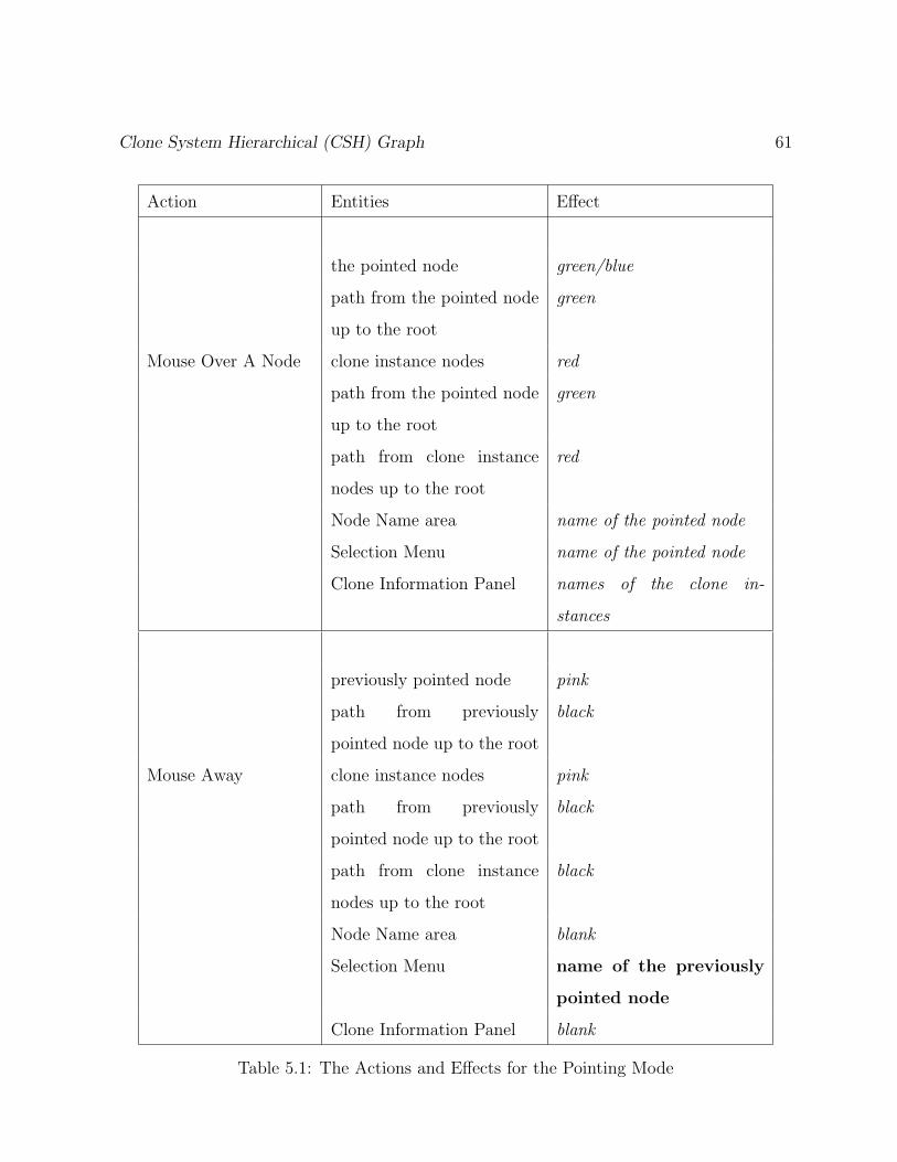
Clone System Hierarchical (CSH) Graph 61
Action Entities Effect
Mouse Over A Node
the pointed node green/blue
path from the pointed node
up to the root
green
clone instance nodes red
path from the pointed node
up to the root
green
path from clone instance
nodes up to the root
red
Node Name area name of the pointed node
Selection Menu name of the pointed node
Clone Information Panel names of the clone in-
stances
Mouse Away
previously pointed node pink
path from previously
pointed node up to the root
black
clone instance nodes pink
path from previously
pointed node up to the root
black
path from clone instance
nodes up to the root
black
Node Name area blank
Selection Menu name of the previously
pointed node
Clone Information Panel blank
Table 5.1: The Actions and Effects for the Pointing Mode
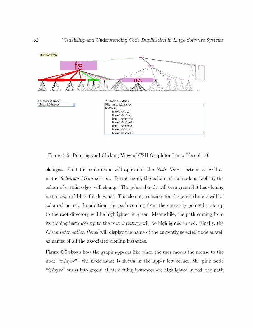
62 Visualizing and Understanding Code Duplication in Large Software Systems
1. Choose A Node:Linux-1.0/fs/sysv
2. Cloning BuddiesFile: linux-1.0/fs/sysvbuddies:
linux-1.0/fs/extlinux-1.0/fs/nfslinux-1.0/fs/xiafslinux-1.0/fs/msdoslinux-1.0/fs/ext2linux-1.0/fs/minixlinux-1.0/fs/isofs
Figure 5.5: Pointing and Clicking View of CSH Graph for Linux Kernel 1.0.
changes. First the node name will appear in the Node Name section; as well as
in the Selection Menu section. Furthermore, the colour of the node as well as the
colour of certain edges will change. The pointed node will turn green if it has cloning
instances; and blue if it does not. The cloning instances for the pointed node will be
coloured in red. In addition, the path coming from the currently pointed node up
to the root directory will be highlighted in green. Meanwhile, the path coming from
its cloning instances up to the root directory will be highlighted in red. Finally, the
Clone Information Panel will display the name of the currently selected node as well
as names of all the associated cloning instances.
Figure 5.5 shows how the graph appears like when the user moves the mouse to the
node “fs/sysv”: the node name is shown in the upper left corner; the pink node
“fs/sysv” turns into green; all its cloning instances are highlighted in red; the path
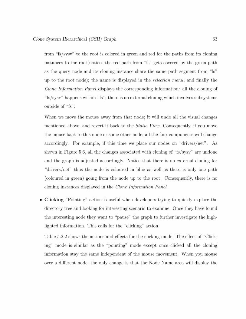
Clone System Hierarchical (CSH) Graph 63
from “fs/sysv” to the root is colored in green and red for the paths from its cloning
instances to the root(notices the red path from “fs” gets covered by the green path
as the query node and its cloning instance share the same path segment from “fs”
up to the root node); the name is displayed in the selection menu; and finally the
Clone Information Panel displays the corresponding information: all the cloning of
“fs/sysv” happens within “fs”; there is no external cloning which involves subsystems
outside of “fs”.
When we move the mouse away from that node; it will undo all the visual changes
mentioned above, and revert it back to the Static View. Consequently, if you move
the mouse back to this node or some other node; all the four components will change
accordingly. For example, if this time we place our nodes on “drivers/net”. As
shown in Figure 5.6, all the changes associated with cloning of “fs/sysv” are undone
and the graph is adjusted accordingly. Notice that there is no external cloning for
“drivers/net” thus the node is coloured in blue as well as there is only one path
(coloured in green) going from the node up to the root. Consequently, there is no
cloning instances displayed in the Clone Information Panel.
• Clicking “Pointing” action is useful when developers trying to quickly explore the
directory tree and looking for interesting scenario to examine. Once they have found
the interesting node they want to “pause” the graph to further investigate the high-
lighted information. This calls for the “clicking” action.
Table 5.2.2 shows the actions and effects for the clicking mode. The effect of “Click-
ing” mode is similar as the “pointing” mode except once clicked all the cloning
information stay the same independent of the mouse movement. When you mouse
over a different node; the only change is that the Node Name area will display the
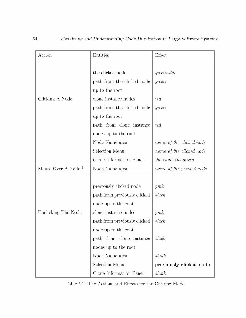
64 Visualizing and Understanding Code Duplication in Large Software Systems
Action Entities Effect
Clicking A Node
the clicked node green/blue
path from the clicked node
up to the root
green
clone instance nodes red
path from the clicked node
up to the root
green
path from clone instance
nodes up to the root
red
Node Name area name of the clicked node
Selection Menu name of the clicked node
Clone Information Panel the clone instances
Mouse Over A Node 1 Node Name area name of the pointed node
Unclicking The Node
previously clicked node pink
path from previously clicked
node up to the root
black
clone instance nodes pink
path from previously clicked
node up to the root
black
path from clone instance
nodes up to the root
black
Node Name area blank
Selection Menu previously clicked node
Clone Information Panel blank
Table 5.2: The Actions and Effects for the Clicking Mode
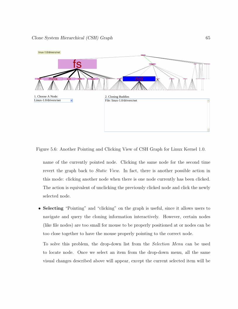
Clone System Hierarchical (CSH) Graph 65
1. Choose A Node:Linux-1.0/drivers/net
2. Cloning BuddiesFile: linux-1.0/drivers/net
Figure 5.6: Another Pointing and Clicking View of CSH Graph for Linux Kernel 1.0.
name of the currently pointed node. Clicking the same node for the second time
revert the graph back to Static View. In fact, there is another possible action in
this mode: clicking another node when there is one node currently has been clicked.
The action is equivalent of unclicking the previously clicked node and click the newly
selected node.
• Selecting “Pointing” and “clicking” on the graph is useful, since it allows users to
navigate and query the cloning information interactively. However, certain nodes
(like file nodes) are too small for mouse to be properly positioned at or nodes can be
too close together to have the mouse properly pointing to the correct node.
To solve this problem, the drop-down list from the Selection Menu can be used
to locate node. Once we select an item from the drop-down menu, all the same
visual changes described above will appear, except the current selected item will be
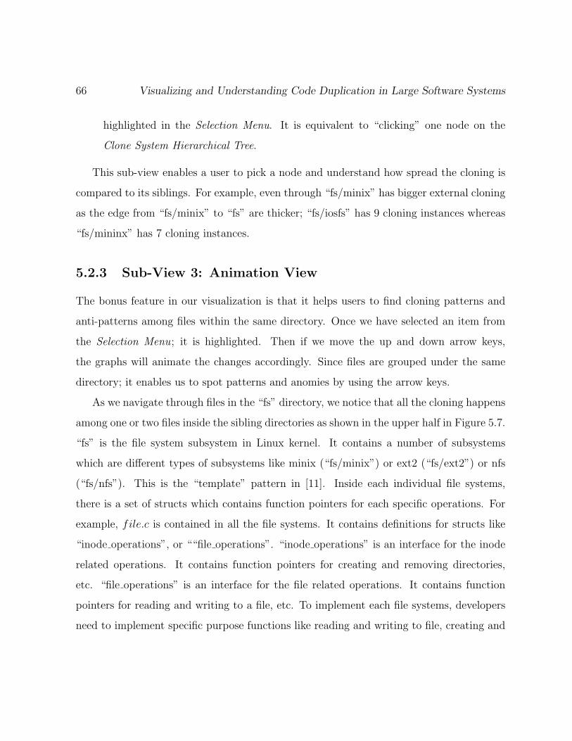
66 Visualizing and Understanding Code Duplication in Large Software Systems
highlighted in the Selection Menu. It is equivalent to “clicking” one node on the
Clone System Hierarchical Tree.
This sub-view enables a user to pick a node and understand how spread the cloning is
compared to its siblings. For example, even through “fs/minix” has bigger external cloning
as the edge from “fs/minix” to “fs” are thicker; “fs/iosfs” has 9 cloning instances whereas
“fs/mininx” has 7 cloning instances.
5.2.3 Sub-View 3: Animation View
The bonus feature in our visualization is that it helps users to find cloning patterns and
anti-patterns among files within the same directory. Once we have selected an item from
the Selection Menu; it is highlighted. Then if we move the up and down arrow keys,
the graphs will animate the changes accordingly. Since files are grouped under the same
directory; it enables us to spot patterns and anomies by using the arrow keys.
As we navigate through files in the “fs” directory, we notice that all the cloning happens
among one or two files inside the sibling directories as shown in the upper half in Figure 5.7.
“fs” is the file system subsystem in Linux kernel. It contains a number of subsystems
which are different types of subsystems like minix (“fs/minix”) or ext2 (“fs/ext2”) or nfs
(“fs/nfs”). This is the “template” pattern in [11]. Inside each individual file systems,
there is a set of structs which contains function pointers for each specific operations. For
example, file.c is contained in all the file systems. It contains definitions for structs like
“inode operations”, or ““file operations”. “inode operations” is an interface for the inode
related operations. It contains function pointers for creating and removing directories,
etc. “file operations” is an interface for the file related operations. It contains function
pointers for reading and writing to a file, etc. To implement each file systems, developers
need to implement specific purpose functions like reading and writing to file, creating and
Clone System Hierarchical (CSH) Graph 67
Pattern1. Choose A Node:linux-1.0/fs/nfs/dir.c
2. Cloning BuddiesFile: linux-1.0/fs/nfs/dir.cbuddies:
linux-1.0/fs/ext2/inode.clinux-1.0/fs/ext/namei.clinux-1.0/fs/xiafs/namei.clinux-1.0/fs/ext/inode.clinux-1.0/fs/minix/inode.clinux-1.0/fs/sysv/inode.clinux-1.0/fs/sysv/namei.clinux-1.0/fs/minix/namei.clinux-1.0/fs/ext2/namei.clinux-1.0/fs/isofs/inode.clinux-1.0/fs/xiafs/inode.c
Pattern
1. Choose A Node:linux-1.0/fs/nfs/mmap.c
2. Cloning BuddiesFile: linux-1.0/fs/nfs/mmap.cbuddies:
linux-1.0/mm/mmap.clinux-1.0/mm/memory.c
Anti-Pattern
Figure 5.7: Animation View of CSH Graph for Linux Kernel 1.0.

68 Visualizing and Understanding Code Duplication in Large Software Systems
removing a file; then set the appropriate function points to these functions in the struct.
Thus, “file.c” in one file system is similar to “file.c” in other file systems.
However, the pattern does not apply to “fs/nfs/mmap.c”. As it does not have any
cloning instances from files within the “fs” directory. Furthermore, as displayed in the
lower half of Figure 5.7, it shares common code with files from the top level “mm”(memory
management) directory! It is a bit surprising since not all file systems contains file mmap.c.
The source code comments of this file states that code is borrowed from “mm/mmap.c”
and “mm/memory.c”; which explains the cloning relations.
5.3 Discussion and Future Work
Comparison with CCC Graph: The CSH graph embeds the cloning information
within a directory tree. The dimension of the nodes implies clone cohesion and
the thickness of the edges implies clone coupling. Rather than showing the cloning
information just at one level of system hierarchy as in the CCC graph, the CSH
graph contains cloning relations at different levels of abstractions: from file level up
to the top level directories. Its adaptive feature allows users to pick an individual
node and highlights the spread out of the cloning. However, one disadvantage for
the CSH graph is that the notion of coupling is not as well indicated as in the CCC
graph, as we do not know the strength of coupling among various subsystems.
Layout: Over-plotting is the problem when there are too many nodes and edges trying to
fit into limited screen space. An over-plotted graph is hard for human to comprehend.
The CSH graph uses the directory structure as the back-bone to display cloning
information. When system contains too many files and the directory structure is
shallow; our visualization will run into the risk of over-plotting. In the future, we are
Clone System Hierarchical (CSH) Graph 69
going to experiment other layout algorithms, such as the radial layout.
Pruning: As mentioned above, our visualization can run into the risk of over-plotting
when the directory structure is shallow and there are a lot of files contained in the
system. Our approach to solve this problem is to use filtering to remove uninteresting
or redundant information. There are two types of filtering we can use: level filtering
and subsystem filtering.
Level pruning means removing all the nodes and edges if they are below the threshold
value. For example, if the directory tree is 6 levels deep and we set threshold of level
filtering to be 3, then all the nodes and edges that are at levels 4, 5 and 6 are filtered.
This is effective; since the deeper into tree, the more nodes we have. Obviously, the
file level, which is at the lowest level of the trees, contains the largest number of
nodes. We apply level filtering when we are interested to examine cloning relations
among subsystems.
Subsystem pruning means removing all the cloning information which is unrelated to
one specified subsystem. Take Linux Kernel for example. If set subsystem filtering to
be “fs”(file system), then all the cloning relations not related to “fs” will be removed
from the data set. We apply subsystem filtering when we want to closely examine
the cloning details for one subsystem.
Other Applications: Depending on the information embedded, this graph can be used
for other purposes as well. For example, we can display the dependency graph or the
co-change graph using the same visualization technique.

70 Visualizing and Understanding Code Duplication in Large Software Systems
5.4 Usage Guideline
We summarize the steps for using our visualization. Researchers can follow this guideline
to process, visualize and analyze cloning for other software systems.
Overall: The CSH graph shows the details of cloning at every level of system abstraction
as well as highlighting the spread of cloning for each individual file and directory.
Data Processing: When we lifting the clone classes, if it is an internal clone class at
the lower level; upon lifting it will still be an internal clone class. For external cloning
classes, if all the entities in the set are under the same parent directory; then it will
become an internal cloning class after lifting. Otherwise, it is an external cloning
class.
Graph Analysis: We summarize the different functions of each sub-view and discuss
a few aspects in the graph that require attention:
Static View is the view when the graph initialized. We get an overview of how
deep the directory structure is, how many entities are actually contained in this
graph.
Pointing and Clicking View enables user to highlight cloning relations for
individual nodes. We need to pay special attentions to the following nodes:
wider nodes since they contain some big internal clone class; thinner nodes
since they contain many small internal clone classes; nodes which have thicker
edges coming out can be alarming as well, since it contains large number of
external cloning.
Animation View allows us to quickly spot the cloning patterns and anomalies
by using the drop down selection menu.
Clone System Hierarchical (CSH) Graph 71
In addition, researchers need to consult other references, such as documentations, the
source code itself, and static dependencies, etc., to uncover the rationale behind cloning.
5.5 Conclusion
This chapter proposes Clone System Hierarchical (CSH) graph, which lays out code cloning
information in a directory tree. It shows code cloning relations at different system abstrac-
tion level varying from the file level, lower-level-subsystem level, and all the way up to the
top-level-subsystem level. In addition, it highlights individual cloning relations for each
files or subsystems by mouse movements.

Chapter 6
Clone System Evolution (CSE)
Graph
This chapter proposes visualization techniques to help researchers to study software evo-
lution. The visualization techniques are ULOC plot, which examines the evolution of
unique features and Clone System Evolution (CSE) graph, which highlights changes in
code cloning over time.
To fully understand code cloning, researchers want to see how current cloning situations
are and why clones evolve to this stage. The previous two views (Clone Cohesion and
Coupling (CCC) graph and Clone System Hierarchical (CSH) graph) focus on visualizing
clones for single software release. We consider them to be snapshot views. They are
important since we need to know the severity of code duplication of current software
system.
To answer why the system ends up with such cloning situation, we need to study how
clones evolve over time, especially the cases when there are lots of clones gets added or
removed. For example, if many clones are added over a short period of time; then we may
72
Clone System Evolution (CSE) Graph 73
wish to investigate the effects on code quality. If many clones are removed, then we need
to be careful since there might be a major refactoring occurred and the interface or system
documentation need to be updated accordingly.
This chapter is organized as follows: Section 6.1 motivates the clone evolution study by
showing the evolution of system growth with or without cloning. Section 6.2 explains our
visualization technique, which highlights the clone changes over time. Section 6.2.4 presents
some discussion about the clone evolution. Finally, section 6.3 gives a short guideline for
researchers who are interested in using our visualization.
6.1 Software Evolution
Software systems evolve over time to accommodate changes such as introduction to new
features, modifications for bug fixes and support for additional platforms, etc.
There are two schools of thoughts about the software development models: the tradi-
tional in-house commercial software development and the open source development model.
It happens that the in-house commercial software development has longer release cycles.
For example Microsoft releases new version of Windows every two or three years. In
addition, they impose tighter coding guidelines. For example, companies like IBM require
developers to prefix their variable names with the module names; some companies even
require strict code ownership: developers need to ask for permission if they want to modify
certain parts of the code which are not owned by them. Furthermore, they incorporate
strict quality assurance procedures before they release their product. Finishing products
are evaluated on a number of aspects such as peer code review, functionality testing,
regression testing, etc.
On the other hand, open source development often seems to takes an opposite approach:
74 Visualizing and Understanding Code Duplication in Large Software Systems
as most of the developers are volunteer based; it has a less strict release schedule since it
would be hard to force volunteer to work hard to meet up the deadlines. Furthermore,
since developers contribute to the project according to their interest; it would be hard to
incorporate the idea of code ownership. What is more, because such projects are volunteer
based, imposing a strict code guidelines would drive away potential contributors. Finally,
since most of the open source developers are also its users; the software incorporates lazy
testing. Lazy testing means software is released without doing any rigorous testing and it
relies on user feedback to report bug. The philosophy behind is called “Linus’s Law” [37]:
“Given enough eyeballs, all bugs are shallow.” User feedbacks should catch most of the
software defects.
Research shows the growth rate for these two development models follows different
models. Lehman et al. [29] devised a set of laws about software evolution based on his
studies on several large E-type legacy software systems, which adopt the in-house commer-
cial software development model. Subsequently, Godfrey et al. [31] studied the evolution
of open source software and discovered that the growth rate does not follows these Laws.
They picked the Linux kernel as their case study and found out that the project grows at
the super-linear rate. Their further analysis shown that one of the subsystems “drivers”
grows at a much faster rate than the rest of subsystems, which is the main reason Linux
follows a much faster growth rate. Robles et al. [19] performed similar case studies on
Linux and a number of other open source software systems. Their results also confirmed
with Godfrey et al.’s findings that the growth of open source software systems do not
follow Lehman’s Law of Software Evolution, which are derived from studies of traditional
commercial software systems. In addition, as pointed in the subsequent work [18], Godfrey
et. al. discovered that “drivers” subsystems have exhibit a large degree of code duplica-
tion. Their findings are: drivers tend to be stand-alone and implement a uniform interface.
Clone System Evolution (CSE) Graph 75
What is more, lots of code copying occur among drivers which come from same hardware
vendors, or interact with same hardware chips or even drivers written by the same devel-
opers, etc. We expect much less cloning happening among commercial software; as they
require a tighter code reviewing policy. So it is quite natural to ask the following question,
how about we perform a control experiment: what is the growth rate of Linux excluding
the cloning factor?
Most of the recent software evolution research papers, such as [31, 19] use SLOC as
the main metric to measure the growth and the complexity of the software systems. In our
study, we introduce the concept of ULOC. ULOC, which measures the number of unique
lines, is different from SLOC, which measures the number source code lines. For example,
if we have two pieces of code segments, which are duplicates of each other; in SLOC we
are going to count both of them whereas in ULOC we are going to count only one of them.
The rest of this section is organized as follows, we are going to first explain our method-
ology and then present a small case study of Linux kernel.
6.1.1 Our Methodology
As the name of ULOC suggests, it is “unique lines of source code”. The idea is simple:
we reduce total lines of source code(SLOC ) by the amount of duplication. It takes two
steps to find the amount of duplicated code: clone data collection, and code duplication
aggregation.
• Calculation of SLOC: In our study, we use a perl script and unix command “wc
-l” to calculate SLOC. There are two main reasons not to choose existing tools like
“sloccount” [40]:
First, this study is intended to compare our findings with existing research, especially
76 Visualizing and Understanding Code Duplication in Large Software Systems
with [31]; so it would be easier to adopt the similar metrics and similar measurement
methods.
Second, as most of the clone detection tools report code duplications using line inter-
vals, we choose the lines of codes with comments to be consistent with the output of
the clone detection tools. These intervals contain source code as well as blank lines
and comments. The perl script we write, recursively searches for the source code files
(.c or .h files); invokes “wc -l” on them and aggregates the results.
• Clone Data Collection: Clone data collection step requires clone detection and
then clone filtering. We choose CCFinder as our clone detection tool and textual
filtering as our filtering technique. The details are described in Section 2.2.
• Code Duplication Aggregation: The next step is to calculate the amount of
duplication. Note that we do want to keep one copy of duplicates. We achieve these
by extracting the information of clone classes. For tools which only outputs clone
pairs, we can form clone classes from the set closure property: as any two elements
in the clone class forms a clone pair. For example, as shown in Figure 1.1, although
(A), (B), and (C) are duplicates of each other and they form a clone class. Then
to obtain the amount of duplicated code, we just need to add up all the duplicated
lines but one. In the above example, we need to pick any two code segments from
(A), (B), and (C) in our calculations. Since each of them have 10 lines duplicated
with each other, thus would be 20 lines counted as duplicated lines.
6.1.2 Examining the Evolution of Linux using ULOC
Previously there have been two parallel releases for the Linux kernel: the stable releases
and the development releases. Stable releases contains relatively less bugs and is preferred
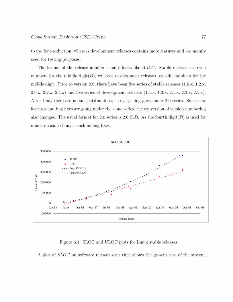
Clone System Evolution (CSE) Graph 77
to use for production; whereas development releases contains more features and are mainly
used for testing purposes.
The format of the release number usually looks like A.B.C. Stable releases use even
numbers for the middle digit(B), whereas development releases use odd numbers for the
middle digit. Prior to version 2.6, there have been five series of stable releases (1.0.x, 1.2.x,
2.0.x, 2.2.x, 2.4.x) and five series of development releases (1.1.x, 1.3.x, 2.1.x, 2.3.x, 2.5.x).
After that, there are no such distinctions; as everything goes under 2.6 series. Since new
features and bug fixes are going under the same series, the conversion of version numbering
also changes. The usual format for 2.6 series is 2.6.C.D. As the fourth digit(D) is used for
minor revision changes such as bug fixes.
SLOC/ULOC
-1000000
0
1000000
2000000
3000000
4000000
5000000
Jan-93 Jun-94 Oct-95 Mar-97 Jul-98 Dec-99 Apr-01 Sep-02 Jan-04 May-05 Oct-06 Feb-08
Release Dates
Line
s of C
ode
SLOCULOCPoly. (SLOC)Linear (ULOC)
Figure 6.1: SLOC and ULOC plots for Linux stable releases
A plot of SLOC on software releases over time shows the growth rate of the system,
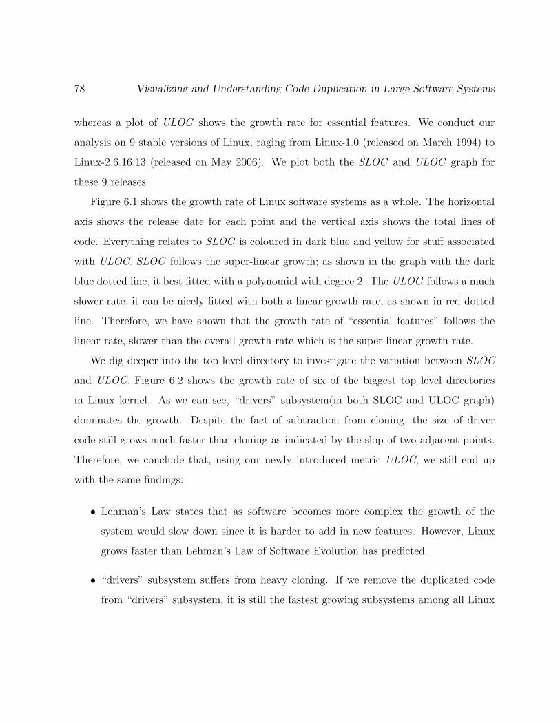
78 Visualizing and Understanding Code Duplication in Large Software Systems
whereas a plot of ULOC shows the growth rate for essential features. We conduct our
analysis on 9 stable versions of Linux, raging from Linux-1.0 (released on March 1994) to
Linux-2.6.16.13 (released on May 2006). We plot both the SLOC and ULOC graph for
these 9 releases.
Figure 6.1 shows the growth rate of Linux software systems as a whole. The horizontal
axis shows the release date for each point and the vertical axis shows the total lines of
code. Everything relates to SLOC is coloured in dark blue and yellow for stuff associated
with ULOC. SLOC follows the super-linear growth; as shown in the graph with the dark
blue dotted line, it best fitted with a polynomial with degree 2. The ULOC follows a much
slower rate, it can be nicely fitted with both a linear growth rate, as shown in red dotted
line. Therefore, we have shown that the growth rate of “essential features” follows the
linear rate, slower than the overall growth rate which is the super-linear growth rate.
We dig deeper into the top level directory to investigate the variation between SLOC
and ULOC. Figure 6.2 shows the growth rate of six of the biggest top level directories
in Linux kernel. As we can see, “drivers” subsystem(in both SLOC and ULOC graph)
dominates the growth. Despite the fact of subtraction from cloning, the size of driver
code still grows much faster than cloning as indicated by the slop of two adjacent points.
Therefore, we conclude that, using our newly introduced metric ULOC, we still end up
with the same findings:
• Lehman’s Law states that as software becomes more complex the growth of the
system would slow down since it is harder to add in new features. However, Linux
grows faster than Lehman’s Law of Software Evolution has predicted.
• “drivers” subsystem suffers from heavy cloning. If we remove the duplicated code
from “drivers” subsystem, it is still the fastest growing subsystems among all Linux
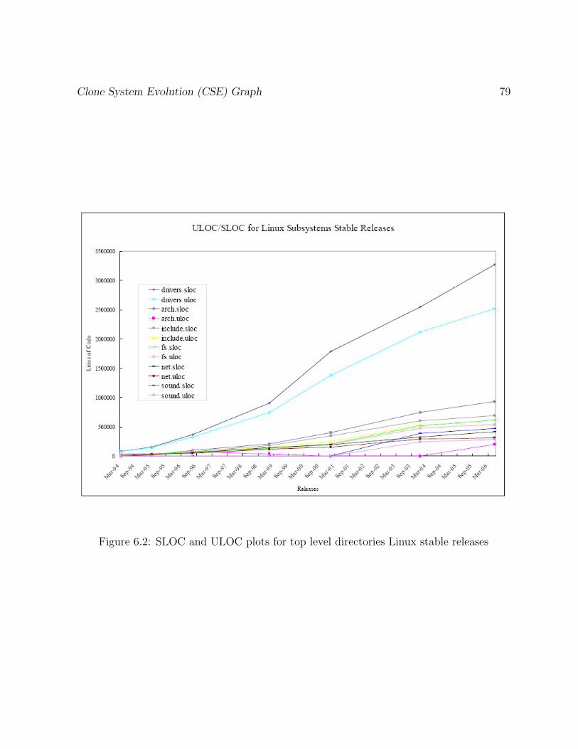
Clone System Evolution (CSE) Graph 79
Figure 6.2: SLOC and ULOC plots for top level directories Linux stable releases
80 Visualizing and Understanding Code Duplication in Large Software Systems
kernel subsystems. The fast growth rate of “drivers” subsystem is main reason caus-
ing the rapid growth rate of Linux compared to traditional in-house software systems.
6.1.3 An Alternative
Compression Size
-10000000
0
10000000
20000000
30000000
40000000
50000000
60000000
Jan-93 Jun-94 Oct-95 Mar-97 Jul-98 Dec-99 Apr-01 Sep-02 Jan-04 May-05 Oct-06 Feb-08
Date
Size
gzip(.c/.h files)tar.gz sizeLinear (gzip(.c/.h files))Poly. (tar.gz size)
Figure 6.3: Plot of Compressed tar.gz File sizes for Linux stable releases.
Because of the enormous size of Linux, it is normally distributed in compressed form.
Most of the compression algorithm reduce file sizes by looking for common patterns among
Clone System Evolution (CSE) Graph 81
files, such as longest common sequence, etc. This idea is somewhat similar as our idea
of ULOC. Therefore, we try to examine the growth rate of compressed tar file size(tar.gz
files). However, this is one little problem: as the available compressed tar files includes
all kinds of files for the Linux kernel, varying from documentation files, source code files,
build configuration files, etc; whereas all of the above experiments have been conducted
on source code files only. So we write a perl script that for each release it groups all the
source code files (.c and .h files) into a tar file and compress the tar file into the gzip file.
Figure 6.3 plots both the original tar.gz files which have everything (shown in pink) and
the tar.gz files which only compress .c and .h files (shown in dark blue). As we can see the
gaps between pink points and dark blue points becomes bigger and bigger indicates more
non-source code files gets added as Linux evolves also these files probably resemble little
similarity thus it becomes harder to compress as the size of the gaps increases over time.
In addition, the growth rate of the compressed source code files can be fitted nicely
with a linear model shown in dark blue. This coincides with our ULOC case study.
6.1.4 Discussion
Motivation for Clone System Evolution Study: We have shown the difference
in system growth rate with(SLOC plot) and without(ULOC plot) account for code
cloning. Code clones are growing at a noticeable rate as the system evolves with
introduction to new features and modifications for bug fixes. Therefore, to fully
uncover the myth of how software systems evolve; it is necessary to study changes in
clones over time.
ULOC as a better metric: SLOC has long been used as an indication of complexity
of the software systems and used for estimating development costs [12]. However, it
82 Visualizing and Understanding Code Duplication in Large Software Systems
is oblivious that the effort to write 100 lines from scratch is different from copying
100 lines and modify based on it. What is more, the cognitive efforts required to
understand two cloning instances is not the same as the time require to decipher two
pieces of code which are totally unrelated. Therefore, we argue ULOC is a better
metric to measure the complexity of the system and to estimate the development
cost.
How To Estimate ULOC: Even though CCFinder is relatively faster than other clone
detection tools, it is still time-consuming to do clone detection on a large software
system. For example, it takes more than 6 hours on a Windows Desktop machine
for CCFinder to do clone detection on one release of 2.6x series. On the other
hand, compressing source code files is much faster. It takes normally minutes to
compress the entire source code directory. In our Linux kernel study, the growth rate
of compressed tar file size coincides with the growth rate of ULOC. In the future, we
are going to verify the co-relation between the size of compressed achieve file sizes
with ULOC on other software systems. If such co-relation exists, we can use the size
of the compression file to predict the growth rate to ULOC.
6.2 Clone System Evolutionary (CSE) Graph
As we can see the system growth rate varies significantly with or without accounting for
code cloning; thus it is important to study the evolution of code cloning to fully under-
stand how the software evolves over time. Our last visualization graph: the Clone System
Evolution (CSE) graph highlights the most recent clone changes from the files all the way
up to the top level subsystems.
The rest of this section covers two components: steps to compute the clone evolutionary
Clone System Evolution (CSE) Graph 83
data and the Clone System Evolution (CSE) graph.
6.2.1 Clone System Evolution Framework
We divide the tasks of computing clone evolutionary data into two steps: Clone System
Hierarchy Extraction and Historical Clone Data Encoding, illustrated in Figure 6.4.
• Clone System Hierarchy Extraction: for each release we perform clone system
hierarchy extraction process. The details are explained in Section 5.1.
• Historical Clone Data Encoding: We now have obtained the clone system
hierarchy information for each release through the development history of the software
project. The challenge comes when we need to visualize the historical information.
The clone system hierarchy information for each release is like a snapshot of the
code duplication situation at one point of time in history. We need to super-impose
these pictures one by one to form the evolutionary view. The result should satisfy
two requirements: first, as cloning information changes from time to time, we need to
reflect the history of changes into our visualization; second, it is would be preferable if
the tool can rank the information and highlight places which are more important and
deemphasizes places which are not so important. We achieve the above requirements
by applying a decay function.
We choose to encode our historical data using a decay function. Decay period refers
to the period of time which information becomes stale, and not interest to us. Half life
is a special kind of decay rate. Half life, originally used in radio-active substances,
refers to the period of time when the mass is only half of the original weight. In
our study, half life can be interpreted as the period of time when the weight of the

84 Visualizing and Understanding Code Duplication in Large Software Systems
Clone Detection
Non-Functional
Clone Filtering
Filtered Clone
ClassesSource Code
Clone Relation
Lifting and Aggregating
Clone System
Architecture
Clone System Architectur Extraction
Version 1
Clone System
Architecture V1
Clone System
Architecture V2
Clone System
Architecture Vn
Historical Clone Data Encoding
Clone Evolutionary
Data
Version 2
Version n
Figure 6.4: Clone Evolutionary Extraction Framework.
Clone System Evolution (CSE) Graph 85
previous releases becomes half. So for example, if the half life is 2 releases, if there
are 200 lines of cloning in the past, it becomes 100 lines in the next release.
Our decay function looks like:
result = (new value− old value) + decay rate ∗ old value;
For example, the old value is 400 and the new value is 500; the decay rate is set to
be 0.2. Then the result computed from the decay function is 180. The decay rate
can be set to different values according to what kind of information users want to
uncover. If users are more interested in the more recent changes, then the decay rate
should be set small, as the information in the past is not so important to us. If users
are more concerned with the cloning history of each entity, the decay rate should be
set to high to preserve the information in the past. Our decay function is applied to
both the internal cloning and the external cloning.
6.2.2 Clone System Evolutionary (CSE) Graph
Once we have encoded all the historical information. We use Clone System Evo-
lutionary (CSE) graph to visualize it. Similar as Clone System Hierarchy View, it
shows all the cloning information in a tree. Additionally, it uses colours to group
and categorize historical cloning information. In this case, we sort subsystems under
the same parent directory by the amount of external cloning from the highest to the
lowest and split them by values into 4 quarters. We assign the entities in the highest
quarter to be red, followed by yellow, light green and grey as shown in Figure 4.3.
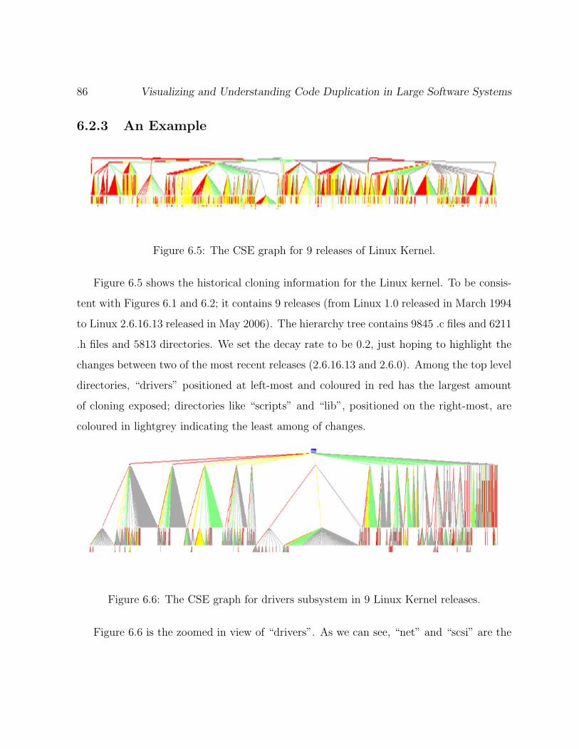
86 Visualizing and Understanding Code Duplication in Large Software Systems
6.2.3 An Example
Figure 6.5: The CSE graph for 9 releases of Linux Kernel.
Figure 6.5 shows the historical cloning information for the Linux kernel. To be consis-
tent with Figures 6.1 and 6.2; it contains 9 releases (from Linux 1.0 released in March 1994
to Linux 2.6.16.13 released in May 2006). The hierarchy tree contains 9845 .c files and 6211
.h files and 5813 directories. We set the decay rate to be 0.2, just hoping to highlight the
changes between two of the most recent releases (2.6.16.13 and 2.6.0). Among the top level
directories, “drivers” positioned at left-most and coloured in red has the largest amount
of cloning exposed; directories like “scripts” and “lib”, positioned on the right-most, are
coloured in lightgrey indicating the least among of changes.
Figure 6.6: The CSE graph for drivers subsystem in 9 Linux Kernel releases.
Figure 6.6 is the zoomed in view of “drivers”. As we can see, “net” and “scsi” are the

Clone System Evolution (CSE) Graph 87
only two of the sub-directories coloured in red and on the right, there are quite a few small
sub-directories such as “bluetooth”, and “macintosh” coloured in grey. We then further
investigate the reasons why there are so many clones get modified in two of the subsystems
“net” and “scsi”.
We wrote a perl script to measure the differences in clone pairs between two versions of
Linux Kernel. The script first extracts the cloning information only relevant to “drivers”.
Then it compares the cloning data in the previous release with the next release. Finally it
classifies the cloning differences into three categories: clones in new files, new clones in old
files, and changes in the old clones, missing clones:
Clones in new files: refer to clone pairs that at least one of the two code segments is
from newly added files. So the clone pairs can be between two newly added files or
between one newly added file and one legacy file.
Missing clones: refer to the clone pairs from which files are removed in the newer
releases. So for example, in the older version, it has one clone pair between “fileA.c”
and “fileB.c”. In the newer version, either “fileA.c” or “fileB.c” or both gets removed.
Therefore, this clone pair no longer exists. We name this type of clones as missing
clones.
New clones in old files: refer to clones in which files exist in both releases but the
cloning relation only appears in the newer release. For example, between “fileA.c”
and “fileB.c”, there is no cloning relations in the older releases but in the newer
release there are code segments from two files which are similar to each other.
Changes in old clones: refer to clones that exist in both releases whose amount of
cloning can stay the same, decrease (existing clones less lines) or increase (existing
clones less lines). So a clone pair which is between “fileA.c” and “fileB.c” exists both
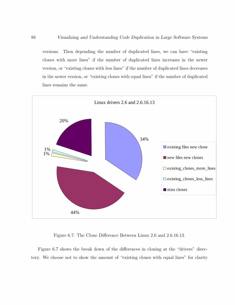
88 Visualizing and Understanding Code Duplication in Large Software Systems
versions. Then depending the number of duplicated lines, we can have “existing
clones with more lines” if the number of duplicated lines increases in the newer
version, or “existing clones with less lines” if the number of duplicated lines decreases
in the newer version, or “existing clones with equal lines” if the number of duplicated
lines remains the same.
Linux drivers 2.6 and 2.6.16.13
34%
20%
1%
44%
1%existing files new clone
new files new clones
existing_clones_more_lines
existing_clones_less_lines
miss clones
Figure 6.7: The Clone Difference Between Linux 2.6 and 2.6.16.13.
Figure 6.7 shows the break down of the differences in cloning at the “drivers” direc-
tory. We choose not to show the amount of “existing clones with equal lines” for clarity
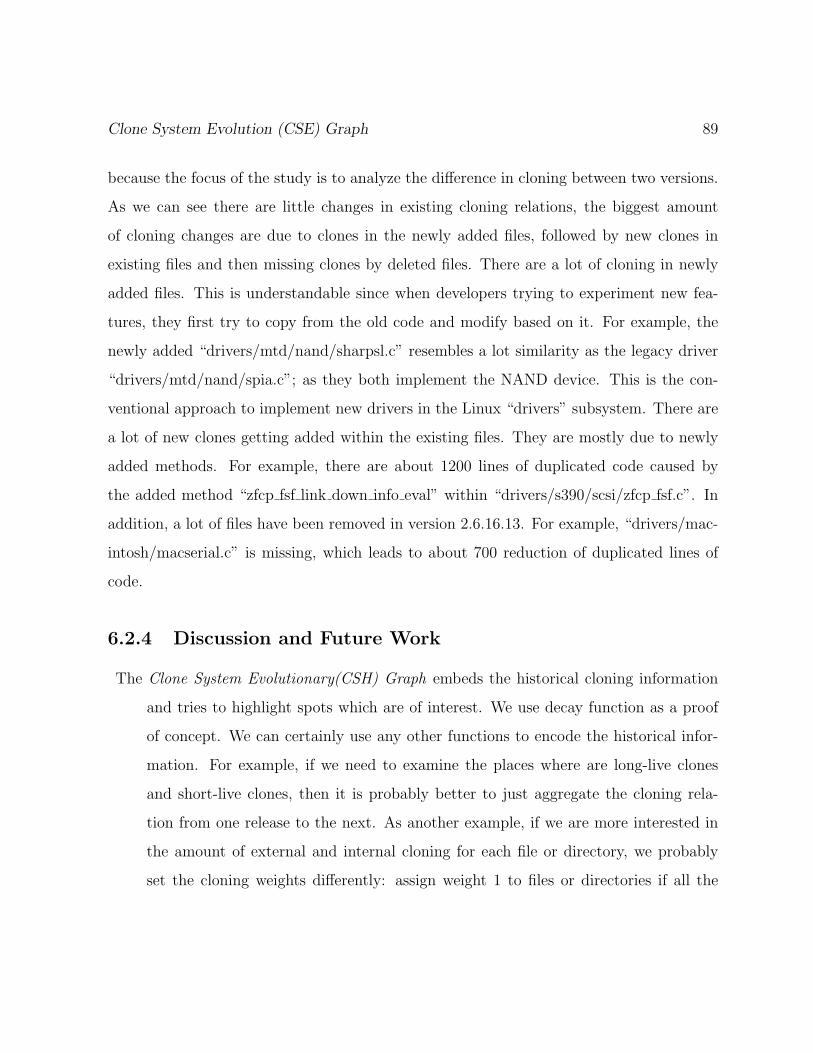
Clone System Evolution (CSE) Graph 89
because the focus of the study is to analyze the difference in cloning between two versions.
As we can see there are little changes in existing cloning relations, the biggest amount
of cloning changes are due to clones in the newly added files, followed by new clones in
existing files and then missing clones by deleted files. There are a lot of cloning in newly
added files. This is understandable since when developers trying to experiment new fea-
tures, they first try to copy from the old code and modify based on it. For example, the
newly added “drivers/mtd/nand/sharpsl.c” resembles a lot similarity as the legacy driver
“drivers/mtd/nand/spia.c”; as they both implement the NAND device. This is the con-
ventional approach to implement new drivers in the Linux “drivers” subsystem. There are
a lot of new clones getting added within the existing files. They are mostly due to newly
added methods. For example, there are about 1200 lines of duplicated code caused by
the added method “zfcp fsf link down info eval” within “drivers/s390/scsi/zfcp fsf.c”. In
addition, a lot of files have been removed in version 2.6.16.13. For example, “drivers/mac-
intosh/macserial.c” is missing, which leads to about 700 reduction of duplicated lines of
code.
6.2.4 Discussion and Future Work
The Clone System Evolutionary(CSH) Graph embeds the historical cloning information
and tries to highlight spots which are of interest. We use decay function as a proof
of concept. We can certainly use any other functions to encode the historical infor-
mation. For example, if we need to examine the places where are long-live clones
and short-live clones, then it is probably better to just aggregate the cloning rela-
tion from one release to the next. As another example, if we are more interested in
the amount of external and internal cloning for each file or directory, we probably
set the cloning weights differently: assign weight 1 to files or directories if all the
90 Visualizing and Understanding Code Duplication in Large Software Systems
clone instances appear to reside under the same directory and 2 if they reside in two
different directories, and so on.
Layout: Developers are more comfortable to visualize the architecture in the directory
structure like framework. However, our visualization technique may not up to scale.
As the number of files increases, it becomes too crowed to fit in the screen. Users
have to zoom in and zoom out to gain a better understanding of certain part of the
diagram. In the future, we are going to experiment with different kinds of layout,
especially the effectiveness of radial layout.
Filtering: Since both the CSH graph and CSE graph use tree structure layout, they
suffer the same over-plotting problem. As there might be too many nodes and files
cramming into the screen. Similar as the CSH graph, we use level filtering and
subsystem filtering to scale down the graph.
Animation: As our view is static, it does not coincide with the dynamic nature of
software evolution. However, one challenge which hinders us from animating the
evolution as the hierarchical view is the “minimal impact” principle. It is preferred
to keep the relative position of directories and files stable, since it is easier for user
to keep track of the changes. However, if one directory gets added or removed how
do we put them without affecting the relative position of other directories and files;
especially in big software systems like Linux which contains millions of files and
thousands of directories? In the future, we are going to look into the ways of of
animating the evolution of code cloning.
Clone System Evolution (CSE) Graph 91
6.3 Guideline
We summarize the steps for using our visualization. Researchers can follow this guideline
to process, visualize and analyze cloning for other software systems.
Overall: The clone evolution graph highlights the most recent changes of cloning in the
system.
Data Processing : We aggregate cloning information across releases. We first create a
directory structure which contains all the directories and files ever existed. Then, we
apply some decaying function to embed the historical information at the file level.
Then we lift the file level information to the subsystem level.
Note that different decay function can be used to highlight different aspects of the
cloning. For example, we can device our decay function to put more values on the
most recent changes or we can instrument the function to put more emphasis on the
spread of the clones, and so on.
Graph Analysis: The graph is highlighted to different colours. Depending on the focus
on the task, we need to pay attention to different entities. In particular the red area
to the left and grey area to the right of the graph.
The most recent biggest clone changes are coloured in red, this can be interesting
since the rationale behind cloning to red nodes can answer questions like: Is cloning
introduced for new features or for bug fixes or something else? If a lot of clones have
been removed, then we want to answer questions like: is there a refactoring or system
restructuring occurred; is there any the interfaces got updated, etc.
For places which have little cloning changes is coloured in grey. They could be
valuable to answer questions like: why there is little cloning changes? Is it due to the
92 Visualizing and Understanding Code Duplication in Large Software Systems
introduction of new clone-free code or is it because that part is relatively stable and
little changes have been performed? If it is due to the addition of clone-free code,
how many call dependencies is introduced to avoid cloning?
Others: The graph of ULOC over releases shows the growth rate of essential features. It
is complementary to the CSE graph, which studies the changes in code duplications.
6.4 Conclusion
This chapter introduces techniques to analyze the evolution of the software systems. The
ULOC plot examines the growth of the essential features; whereas the complementary
Clone System Evolution (CSE) graph displays the most recent changes in code duplications.
Chapter 7
Conclusion and Future Work
This chapter summarizes the main ideas addressed in this thesis and proposes some future
work in the areas of clone evolution and visualization.
As was explained in Chapter 1, clones are identical or near identical segments of code.
Clones can be good or bad depending on the context. Cloning may be desirable since it
speeds up the development process. Reusing the already tested components reduces the
risks. Cloning can be avoidable due to language limitations or performance requirements.
Cloning is bad since it leads to a bloated code base and in term requires more storage spaces.
Clones are considered bad smell for code quality; since it brings challenges for software
maintenance. Many of the above points are drawn either from some user experience or
from the academic research. There is a lack of empirical study on the consequence of code
cloning.
One of the major challenges for studying code clones in large software systems is how to
handle large set of cloing data; as about 5-50% of the source code can be clones [8, 39, 7].
In this thesis, techniques and tools have been proposed to scale down and visualize the
cloning data.
93
94 Visualizing and Understanding Code Duplication in Large Software Systems
7.1 Major Topics Addressed
To scale down the cloning data, we have proposed three types of scaling: abstracting the
data by lifting the cloning relation from the file level to the subsystem level; merging mul-
tiple similar clone classes into one big clone class; and filtering out irrelevant information.
Using the scaled data, we have proposed three types of visualization, ranging from a
snapshot view of how cloning situations are to the evolutionary view showing how clones
evolves over time. Three of our visualizations emphasize cloning along different dimensions:
along the quantity scale: the Clone Cohesion and Coupling (CCC) graph shows the
degree of internal and external cloning among subsystems;
along the relation scale: the Clone System Hierarchy (CSH) graph puts more focus
on the details of cloning, especially the spread of the cloning;
along the time scale: the Clone System Evolution (CSE) graph highlights the most
recent clone changes.
We showcase our visualizations by applying them to a large open source software system:
the Linux Kernel.
7.2 Future Research
First of all, this thesis demonstrates our visualization tools mainly on various case studies
of Linux Kernel. In the future, we plan to work on additional software projects to evaluate
the effectiveness of these three visualization techniques and hope to uncover interesting
clone design patterns.

Conlusion 95
In addition, as the directory tree structure may not up to scale; various layout algo-
rithms, such as radial layout, will be experimented with. Furthermore, as we can apply
different evolution functions in Clone System Evolution (CSE) graph; we plan to devise a
few of these evolution functions and test to see which ones are best suited to explore which
aspects of clone evolution studies.
We are also interested in applying more user studies to verify and improve the effec-
tiveness of our visualizations.
Finally, we may redo Godfrey et. al.’s study [31] but using ULOC to study the growth
rate to a number of open source software systems.
Bibliography
[1] AiSee. http://www.aisee.com/.
[2] A. Chou, J. Yang and B. Chelf and S. Hallem and D. R. Engler. An empirical study of
operating system errors. In In Proceedings of the 18th ACM Symposium on Operating
Systems Principles (SOSP), October 2001.
[3] A. Cox. An Introduction to SCSI Drivers. Available online at
http://www.linux-mag.com/1999-08/gear 01.html.
[4] A. Monden and D. Nakae and T. Kamiya and S. Sato and K. Matsumoto. Software
quality analysis by code clones in industrial legacy software. In In Proceedings of
IEEE Symposium on Software Metrics 2002, 2002.
[5] I. Baxter, A. Yahin, L. Moura, M. Sant’Anna, and L. Bier. Clone Detection Us-
ing Abstract Syntax Tree. In Proceedings of Sixth Working Conference on Reverse
Engineering), November 1998.
[6] Ivan T. Bowman, Richard C. Holt, and Neil V. Brewster. Linux as a Case Study: Its
Extracted Software Architecture. In Proceedings of the 21st International Conference
on Software Engineering, Los Angeles, USA, May 1999.
96

Conlusion 97
[7] Bruno Lague, Daniel Proulx, Jean Mayrand, Ettore Merlo, John P. Hudepohl. Assess-
ing the Benefits of Incorporating Function Clone Detection in a Development Process.
In Proceedings of the International Conference on Software Maintenance(ICSM1997),
pages 314–321, 1997.
[8] B.S. Baker. On finding duplication and nearduplication in large software system. In
Proceedings of Second IEEE Working Conference on Reverse Eng. (WCRE 1995),
July 1995.
[9] E. Burd and J. Bailey. Evaluating clone detection tools for use during preventative
maintenance. In Second IEEE International Workshop on Source Code Analysis and
Manipulation (SCAM’02), pages 36–43, 2002.
[10] A. Chou, J. Yang, B. Chelf, S. Hallem, and D. R. Engler. An empirical study of
operating system errors. In In Proceedings of the 18th ACM Symposium on Operating
Systems Principles (SOSP), pages 73–88, Banff, Alberta, Canada, October 2001.
[11] Cory Kapser and Michael W. Godfrey. Cloning Considered Harmful’ Considered
Harmful. In Proceedings of the 2006 Working Conference on Reverse Engineering
(WCRE-06), Benevento, Italy, October 2006.
[12] More Than a Gigabuck: Estimating GNU/Linux’s Size. Available online at
http://www.dwheeler.com/sloc/.
[13] Exuberant Ctags. Available online at http://ctags.sourceforge.net.
[14] S. Ducasse, M. Rieger, and S. Demeyer. A language independent approach for detect-
ing duplicated code. In Proceedings ICSM99 (International Conference on Software
Maintenance), pages 109–118, 1999.
98 Visualizing and Understanding Code Duplication in Large Software Systems
[15] Ettore Merlo and Michel Dagenais and P. Bachand and J. S. Sormani and Sara
Gradara and Giuliano Antoniol. Investigating Large Software System Evolution: The
Linux Kernel. In In Proceedings of COMPSAC 2002, pages 421–426, 2002.
[16] Richard Fanta and V’aclav Rajlich. Removing clones from the code. Journal on
Software Maintenance and Evolution, 11(4):223C243, July/Aug 1999.
[17] David Garlan and Mary Shaw. An Introduction to Software Architecture. In V. Am-
briola and G. Tortora, editors, Advances in Software Engineering and Knowledge En-
gineering, pages 1–39, Singapore, 1993. World Scientific Publishing Company.
[18] Michael W. Godfrey, Davor Svetinovic, and Qiang Tu. Detecting duplicated and
near duplicated structures in large software systems: methods and applications. In
CASCON workshop, November 2000.
[19] Gregorio Robles and Juan Jose Amor and Jess M. Gonzlez-Barahona and Israel Her-
raiz. Evolution and Growth in Large Libre Software Projects. In Proceedings of the
2005 International Workshop on Software Evolution(IPWSE 2005), pages 165 – 174,
2005.
[20] Hamid Abdul Basit and Damith C. Rajapakse and Stan Jarzabek. Beyond templates:
a study of clones in the STL and some general implications. In In Proceedings of
International Conference on Software Engineering (ICSE 2005), May 2005.
[21] J. Helfman. Dotplot Patterns: a Literal Look at Pattern Languages. In TAPOS, pages
31–41, 1995.
[22] James R. Cordy. Comprehending Reality: Practical Challenges to Software Main-
tenance Automation. In In Proceedings of IEEE 11th International Workshop on
Program Comprehension, IPWC 2003 (Keynote paper), May 2003.
Conlusion 99
[23] J. H. Johnson. Visualizing textual redundancy in legacy source. In In Proceedings of
CASCON 94, pages 9–18, 1994.
[24] J. H. Johnson. Navigating the textual redundancy web in legacy source. In In Pro-
ceedings of the 1996 conference of the Centre for Advanced Studies on Collaborative
research, 1996.
[25] Toshihiro Kamiya, Shinji Kusumoto, and Katsuro Inoue. CCFinder: A Multi-
Linguistic Token-based Code Clone Detection System for Large Scale Source Code.
IEEE Transactions on Software Engineering, 28(7):654–670, july 2002.
[26] Cory J. Kapser and Michael W. Godfrey. Supporting the Analysis of Clones in Soft-
ware Systems: A Case Study. Journal of Software Maintenance and Evolution: Re-
search and Practice, 18(2), 2006.
[27] Miryung Kim, Vibha Sazawal, David Notkin, and Gail C. Murphy. An empirical study
of code clone genealogies. In ESEC/SIGSOFT FSE 2005, pages 187–196, 2005.
[28] Kostas Kontogiannis. Evaluation Experiments on the Detection of Programming Pat-
terns Using Software Metrics. In Proceedings of the Fourth Working Conference on
Reverse Engineering(WCRE1997), 1997.
[29] M. M. Lehman and J. F. Ramil and P. D. Wernick and D. E. Perry and W. M. Turski.
Metrics and laws of software evolutionthe nineties view. In Proceedings of the Fourth
Intl. Software Metrics Symposium (Metrics97), Albuquerque, NM, 2001.
[30] Magiel Bruntink and Arie van Deursen and Tom Tourwe and Remco van Engelen. An
Evaluation of Clone Detection Techniques for Identifying Crosscutting Concerns. In
In Proceedings of ICSM 2004, pages 200–209, 2004.
100 Visualizing and Understanding Code Duplication in Large Software Systems
[31] Michael W. Godfrey and Qiang Tu. Evolution in open source software: A case study.
In Proceedings of the 16th International Conference on Software Maintenance, pages
131–142, San Jose, California, October 2000.
[32] Miryung Kim and Lawrence D. Bergman and Tessa A. Lau and David Notkin. An
Ethnographic Study of Copy and Paste Programming Practices in OOPL. In Inter-
national Symposium on Empirical Software Engineering(ISESE 2004), August 2004.
[33] B.S. Mitchell and S. Mancordis. On the Automatic Modularization of Software Sys-
tems Using the Bunch Tool. IEEE TSE, 32(3):193–208, 2006.
[34] Raghavan Komondoor and Susan Horwitz. Eliminating duplication in source code via
procedure extraction.
[35] Raihan Al-Ekram and Cory Kapser and Richard Holt and Michael Godfrey. Cloning
by Accident: An Empirical Study of Source Code Cloning Across Software Systems. In
Proceedings of the 2005 Intl. Symposium on Empirical Software Engineering (ISESE-
05), Noosa Heads, Australia, 2005.
[36] Rainer Koschke. Software Clone Detection Survey. In Daugstuhl Seminar Duplication,
Redundancy, and Similarity in Software, July 2006.
[37] Eric S. Raymond. Cathedral and the Bazaar: Musings on Linux and Open Source by
an Accidental Revolutionary. O’Reilly Media, 2001.
[38] Matthias Rieger, Stphane Ducasse, and Michele Lanza. Insights into System-Wide
Code Duplication. In WCRE 2004, pages 100–109, 2005.
Conlusion 101
[39] S. Ducasse and M. Rieger and S. Demeyer. A language independent approach for de-
tecting duplicated code. In Proceedings of IEEE Internaltional Conference on Software
Maintenance(ICSM 1999), August 1999.
[40] SLOCCount. Available online at http://www.dwheeler.com/sloccount/.
[41] T. Fruchterman and E. Reingold. Graph drawing by force-directed placement. page
1129C1164, 1991.
[42] Michael Toomim, Andrew Begel, and Susan L. Graham. Managing Duplicated Code
with Linked Editing. In VL/HCC 2004, pages 173–180, 2004.
[43] Yasushi Ueda, Yoshiki Higo, Toshihiro Kamiya, Shinji Kusumoto, and Katsuro Inoue.
Gemini: Code clone analysis tool. In Proc. of 2002 International Symposium on
Empirical Software Engineering (ISESE2002), Nara, Japan, Oct 2002.