Visualizing Astronomical Data with Blender

Brian R. Kent

National Radio Astronomy Observatory1

520 Edgemont Road, Charlottesville, VA, 22903, USA

Email: bkent@nrao.edu

Web: http://www.cv.nrao.edu/∼bkent/computing/kentPASP.html

-

Published in the Publications of the Astronomical Society of the Pacific

ABSTRACT

Astronomical data take on a multitude of forms – catalogs, data cubes, images, and

simulations. The availability of software for rendering high-quality three-dimensional

graphics lends itself to the paradigm of exploring the incredible parameter space afforded

by the astronomical sciences. The software program Blender gives astronomers a useful

tool for displaying data in a manner used by three-dimensional (3D) graphics special-

ists and animators. The interface to this popular software package is introduced with

attention to features of interest in astronomy. An overview of the steps for generating

models, textures, animations, camera work, and renders is outlined. An introduction is

presented on the methodology for producing animations and graphics with a variety of

astronomical data. Examples from sub-fields of astronomy with different kinds of data

are shown with resources provided to members of the astronomical community. An

example video showcasing the outlined principles and features is provided along with

scripts and files for sample visualizations.

Subject headings: Data Analysis and Techniques

1. Introduction

The combination of astronomy and computational sciences plays an important role in how

members of the astronomical community visualize their data. Larger detectors in the optical/infrared

(IR), increasing bandwidth in radio/millimeter interferometers, and large N astrophysical simula-

tions drive the need for visualization solutions. These visualization purposes include exploring the

dynamical phase space of data cubes, surface mapping, large catalogs, and volumetric rendering.

1The National Radio Astronomy Observatory is a facility of the National Science Foundation operated under

cooperative agreement by Associated Universities, Inc.

– 2 –

The use of 3D computer graphics in the movie, television, and gaming industry has led the de-

velopment of useful computer algorithms for optimizing the display of complex data structures

while taking advantage of new hardware paradigms like utilizing graphic processing units (GPUs).

Melding the exciting scientific results with state of the art computer graphics not only helps with

scientific analysis and phase space discovery, but also with graphics for education and public out-

reach. Exploratory data visualization can offer a complementary tool next to traditional statistics

(Goodman 2012). The work presented here is motivated by a dearth of clear instruction for as-

tronomers in 3D graphics, animation, and accessible visualization packages. The visual impact of

astronomy cannot be understated – for both the community of scientists and how to present our

results to the public with higher accuracy.

We present a practical overview for astronomers to the capabilities of the software program

Blender – an open-source 3D graphics and animation package. We take the approach of describing

the features that will be of interest to various parties in astronomy – for both research visualiza-

tion and presentation graphics. We aim to describe methods of data modeling, texturing, lighting,

rendering, and compositing. Section 2 discusses some of the relevant history of data visualization

in the sciences. Section 3 introduces the software, interface, and workflow. Section 4 describes

the methodology of a sample workflow session using an astronomical position-position-frequency

data cube at radio frequencies. Section 5 describes examples from different fields within astron-

omy. Section 6 summarizes the method overview and includes a demonstration video outlining the

foundations and examples built upon in this paper.

2. Visualizing Data in the Sciences

Three-dimensional visualization allows for the exploration of multiple dimensions of data and

seeing aspects of phase space that may not be apparent in traditional two-dimensional (2D) plotting

typically used in analysis. Visualizing scientific data helps to complement the narrative of an

observation or experiment. A number of studies have reviewed the progression and evolution of

the field in software engineering and the sciences (Staples & Bieman 1999; Wainer & Velleman

2001; Diehl 2007; Teyseyre & Campo 2009). Beginning with the first graphs and charts of analog

mapping data (Robinson 1982), data visualization has grown as technology now allows us to explore

multiple dimensions of parameter spaces. Friendly (2006) gives an overview of visual thinking and

data presentation in mathematics, statistics, and the sciences. Hansen & Johnson (2005) describe

the computer graphics nomenclature, techniques of volume rendering, frameworks, and issues of

perception in visualization.

The field of visualization in the physical sciences, including astronomy, faces challenges of

scalability (Yost & North 2006). Technology only brings us part of the way toward successfully

understanding how to best visualize scientific data – understanding the theory of light, reflection,

and color in graphics is needed to produce useful results (Frenkel 1988). In addition, using a

workflow and framework that maximizes the use of layers and node composition can optimize

– 3 –

the visualization of data (Birn 2000). The goals of scientific visualization are twofold, as are the

underlying challenges – we want to analyze quantitatively with high accuracy and precision our

experiments, but at the same time produce stunning visuals that convey results beyond the scientific

community (Munzner et al. 2006).

Notable usage of scientific visualization, particularly with Blender, include the animation of

maps from geographic information systems(GIS; Scianna 2013), biology (Autin et al. 2012), and

protein models (Zini et al. 2010). Algorithm development in medical imaging has paved the way

in visualizing tomography and magnetic resonance (Lorensen & Cline 1987). Drebin et al. (1988),

Elvins (1992), and Yagel (1996) list early reviews, developments, and taxonomy of algorithms for

volume rendering and viewing, many of which started in the film and animation industry. While

applications may be particular to specific science sub domains, the data and visualization goals

are often similar and well aligned (Borkin et al. 2007). Lipsa et al. (2012) reviews the literature

across the different physical sciences, breaking down visualization into the areas of 2D, 3D, and

time-series data analyses.

With the advent of large sky surveys across the electromagnetic spectrum, short cadence

temporal observations, and high-resolution simulations, astronomy now requires innovative use

of software to analyze data (Turk et al. 2011). These data and methodologies can be catalogs

(Buddelmeijer & Valentijn 2013; Jacob & Plesea 2001; Taylor et al. 2011), images (Bertin & Arnouts

1996; Lupton et al. 2004; Levay 2011), multidimensional datacubes (Draper et al. 2008; Kent 2011),

spectra and time-series (Leech & Jenness 2005; Bergeron & Foulks 2006; Mercer & Klimenko 2008),

and simulations (Teuben et al. 2001). New techniques are utilizing high-performance computing

and access to distributed data (Strehl & Ghosh 2002; Comparato et al. 2007). Volume rendering,

lighting, and shading play a key roll in how data are presented (Gooch 1995; Ament et al. 2010;

Moloney et al. 2011). Still, other experiments require new algorithms or innovative uses of existing

hardware to push through challenging roadblocks that arise with new scientific paradigms (Wenger

et al. 2012; Kuchelmeister et al. 2012). Hassan & Fluke (2011) review different approaches in

astronomy looking to the future of the field as data rates increase.

This work examines how astronomers can use the 3D graphics software Blender to visualize

different types of astronomical data for purposes of both research and education and public outreach.

We briefly compare Blender to other 3D packages in section 3.6. Using a 3D graphics package gives

control over the 4th dimension of many datasets – namely time when animating videos. In addition,

cinematic camera mechanisms and object manipulation used during rendering can give control other

packages cannot (Balakrishnan & Kurtenbach 1999). While there is a wealth of specialized software

libraries and algorithms available, we choose to introduce Blender to astronomers for its versatility

and flexibility in handling different types of visualization scenarios in astronomy.

– 4 –

3. Blender

Blender is a software package aimed at supporting high-resolution production quality 3D graph-

ics, modeling, and animation. The open-source software is maintained by the Blender Foundation

with a large user base and over 3.4 million downloads per year1. The official release under the GNU

GPL is available for Linux (source and pre-built binaries), Mac OS X, and Windows on 32-bit and

64-bit platforms. The graphical user interface (GUI) is designed and streamlined around an ani-

mator’s production workflow with a Python application program interface (API) for scripting. The

API is advantageous in astronomy for loading data through PYFITS or CFITSIO as well as the

growing collection of Python modules available for astronomy. The final composited output can be

high-resolution still frames or video. While the package has numerous uses for game theory and

design, video editing, and graphics animation, here we focus on the components most applicable

to scientific visualization in astronomy. As an existing stand alone software package Blender pro-

vides a framework for both astronomical data exploration as well as education and public outreach.

Motivations for usage in astronomy can be for exploratory data analysis by rendering volumetric

data cubes, projecting and mapping onto mesh surfaces, 3D catalog exploration, and animating

simulation results. Blender meets the requirements for both audiences – that of rigorous scientific

accuracy in addition to the fluid cinema animations that bring the visual excitement of astronomy

to the public.

3.1. Interface and Workflow

The main Blender interface is shown in Figure 1 and shows the object toolbar, main 3D view-

port, transformation toolbar, data and model outliner, properties panel, and animation time line.

A typical session workflow in 3D animation consists of the following steps:

Modeling. The user generates models, called meshes, that conform to the type of data they

wish to view (Figure 2). Fundamental mesh primitives can act as data containers (for 3D data

cubes), volumes (for gas flow simulations), 3D data points (for N -body simulations) or surfaces

(for planetary surface maps). These shapes can morph and change their location, rotation, and scale

during animation (Figure 3). Each mesh, no matter the size, consists of three basic components

– vertices, edges, and faces. As the properties of these basic components are modified the data

visualization begins to take shape.

Texturing and Mapping. Texturing is no longer limited to simple repetitive patterns of bit-

mapped images on surfaces. Such surface texture mapping can be useful for planetary surfaces. 3D

animation packages use a technique called UV-unwrapping (not to be confused with u-v coordinates

1Available from http://www.blender.org/

– 5 –

used in interferometry). This technique projects surfaces of 3D models onto images (Figure 4)2.

Bump mapping is another useful utility allows the simulation of surface differences using pertur-

bations of the surfaces’ normals during the render stage, where a full 3D model would have been

needed otherwise (Blinn 1978). Blender does not possess the native ability to process astronomi-

cal coordinate headers specified in FITS file headers. Further processing through a Python script

would be required in order to reorient surface models to the correct map projection; however, the

capabilities exist for such endeavors, made easier by the Python API and supporting astronomical

libraries3.

Astronomy data that is multidimensional has signal buried in noise and must use volumetric

texturing. Human perception has the uncanny ability to act as an amazing signal extractor in

one-dimensional spectra or two-dimensional images. However, seeing through a data cube requires

us to allow signal emission to pass through a specified noise level. The computation of a ray as it

passes in and out of one volumetric pixel (a voxel) to the next is given by a simple transfer function

(Levoy 1988):

Cout,RGB(ui, vj) = Cin,RGB(ui, vj)(1 − α(xi, yj , zk)) + c(xi, yj , zk)α(xi, yj , zk) (1)

where Cout,RGB and Cin,RGB are the red, green and blue (RGB) values of entry and exit at

pixel (ui, vj), and α is the opacity. c(xi, yj , zk) represents the color values at the point of interaction.

Viewing this signal while ”seeing through” the noise requires a combination of opacity channels

(called alpha in the graphics industry) and ray tracing. The output pixel projected onto the camera

plane is a composited red, green blue, and alpha (RGBA) rendered image (Porter & Duff 1984). In

addition astrophysical visualization, this paradigm exists in other fields including medical imaging

and examining large microscopy image stacks (Feng et al. 2011; Shahidi et al. 1996; Peng et al.

2010). The paradigm is functionally the same as frequency channels in an astronomical data cube

obtained with a radio telescope. Noncube voxel shapes present an interesting challenge for rendering

algorithms, as some 3D models (or FITS data cube projections in astronomy) are not fundamentally

a simple x-y-z orthogonal projection (Reniers & Telea 2008). The current VoxelData4 base class

in Blender allows for any mesh shape, including non-cubic, to be containers for voxel textures.

This has potential for more complex map projections in astronomical surveys, large scale structure

simulations, adaptive mesh refinement codes (AMR) or tessellation algorithms; it is typically used

in animation for web/sponge-like constructs where coordinates can be mapped more easily onto

non-cubic surfaces (Crassin et al. 2009; Strand & Borgefors 2005).

Lighting. This step specifies how light will reflect, refract, and scatter off of physical surfaces. For

astronomical data we will be concerned with how the data are presented on a graphics display that

2Images available at http://earthobservatory.nasa.gov

3http://stsdas.stsci.edu/astrolib/pywcs/

4blender.org/documentation/blender python api 2 65 release/bpy.types.VoxelData.html

– 6 –

the user will see through the camera viewport. Various lighting algorithms are available depending

on the presentation required (Phong 1975).

Animation. Animation is accomplished by recording a change of state in the mesh models and

their associated properties. This task uses ”keyframing” to record location in 3D space, translation,

rotation, and relative scaling between frames. Keyframe pivot points can rapidly increase in number

- fortunately there is a built in feature, the ”graph editor” that gives a schematic view of movement

during animation. Figure 5 shows the graphical view of a camera location as it tracks an object

during an animation.

Camera Control. In addition to animating the meshes, models, and properties, camera movement

and rotation, focal length, depth of field can be controlled and keyframed. This is one of the most

useful features of Blender – giving the user complete control over how to view the generated

animation. The camera can follow a path past a specified object while tracking a given feature.

The camera can fly an orbit around a data cube, and then move in closer to chosen features. This

utility is made easier in the GUI rather than the scripting mode because the user can see where

the camera is moving relative to the models.

Rendering. Rendering can be handled by a number of internal rendering engines – the code that

takes all the animation movements, textures, and lighting emission and absorption parameters,

and generates the frames of animation, as viewed by the camera (or multiple cameras, for multiple

rendering passes). Blender has two engines that are included by default – called Render and Cycles.

Both serve useful purposes depending on the kind of data visualization being performed. We will

discuss these and other third-party rendering engines in section 3.3.

Compositing. Complex data visualization usually benefits from having the aforementioned data

models, animation, cameras, and render output separated for ease of manipulation. A single image

in a raster graphics program such as Adobe Photoshop or GIMP is normally separated into multiple

layers, channels, and paths to facilitate manipulating transparency, brightness, and saturation. In

the same vein with 3D graphics and animation packages, multiple layers can be combined into the

final animation via the ”node compositing editor.” Using nodes gives the user a tree-based graph

that links layers, models, and any final graphical corrections to the final view output into a map

showing the progression on the final composite (Duff 1985; Brinkmann 2008). In a fashion similar

to layers in astronomical browsing utility Aladin (Boch et al. 2011), separate rendered frames from

different source models can be combined. Final frames can be added together using the ”video

sequence editor” in a variety of standard graphics formats (PNG, GIF, JPEG, and TIF for single

frames, and AVI, H.264, Quicktime, and MPEG for video among many others).

The GUI can change depending on the task at hand (modeling, animation, compositing, or

sequencing), and can be fully customized by the user. Intricate details of using the GUI are

beyond the scope of this introductory paper. The Blender documentation5 and workbooks contain

5Manual available at http://wiki.blender.org/index.php/Doc:2.6/Manual

– 7 –

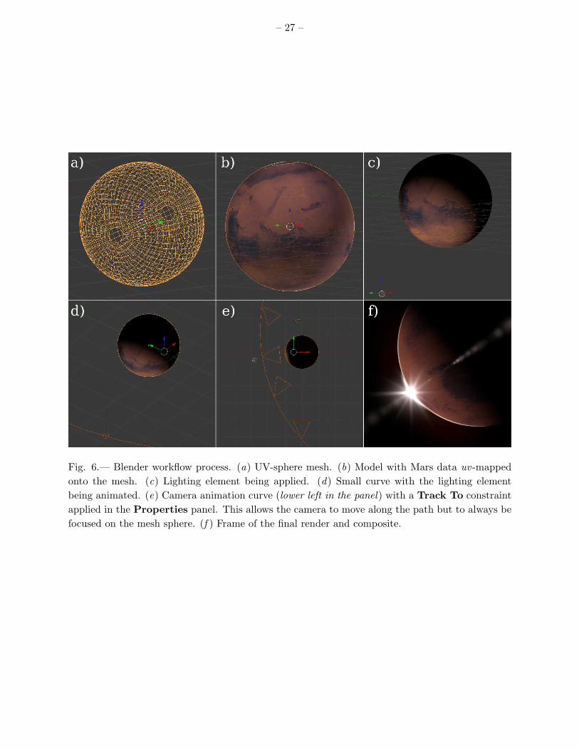
numerous tutorials for learning how to navigate the interface (Hess 2010). Figure 6 shows an outline

of the workflow process from modeling through the final render of a planetary surface map using

data from the NASA Viking Orbiter6.

3.2. Blender Data Structures and Outliner

The Blender core is written in C, with C++ for windowing and Python for the API and

scripting functionality. Native Blender files (*.blend) contain headers with identifiers, pointer sizes,

endianness, and versioning. These headers are followed by data blocks with sub headers containing

identifier codes, data sizes, memory address pointers, and data structure indices. Each block

contains data arrays for object names and types (mesh, light, camera, curve, etc.), data types,

data lengths, and structures, which may contain sub arrays of the fields. The data block for an

animated scene consists of structures detailing objects and their properties - locations of vertices,

edges, faces, and textures, and how those might be affected by a given keyframe. A sample of how

these data structures fit together in the workflow paradigm is shown in Figure 7. Hovering over

any element, button, or menu in the Blender interface gives a context sensitive reference to classes

and methods in the API7. These can be used to write procedural Python scripts for automating

tasks within Blender.

3.3. Rendering Engines

Blender can show real time previews of the animated scene in wireframe, solid, or textured

mode, allowing the user to plan and anticipate when and where camera placements and movements

need to take place. When the render and composite of all layers is required, the Blender data

model is passed to a rendering engine, software that computes the emission, absorption, scattering,

reflection, shading, and transport of simulated light onto the projected camera plane. The following

rendering engines can be used with Blender; this list is not exhaustive, but gives the reader a number

of open-source references to begin exploring different options.

Render. The first generation internal rendering engine is useful for most general purpose data

visualizations that astronomers will encounter. It handles volumetric rendering well and supports

GPU processing (http://wiki.blender.org/index.php/Doc:2.6/Manual/Render).

Cycles. This second generation rendering engine adds more realistic caustics to the rendering algo-

rithm. In addition, the rendering path can be configured within the node-based compositor, allowing

for rapid prototyping of a scene (http://wiki.blender.org/index.php/Doc:2.6/Manual/Render/Cycles).

6Maps available at http://www.mars.asu.edu/data/mdim color/

7API documentation available at http://www.blender.org/education-help/

– 8 –

LuxRender. This open-source third party rendering engine that achieves fast raytracing with

GPU processing and uses a progressive rendering algorithm (see references in Price et al. (2011);

http://www.luxrender.net/ ).

YafaRay. This open-source third party raytracing and rendering engine that has the ability to

save files to high dynamic range images formats (EXR; Debevec 1998, http://www.yafaray.org/ ).

In addition, usage of the utility FFmpeg8 can be used to encode video to popular video formats,

frame rates, from production quality high-definition (HD) video to sizes and data compressions more

suitable to mobile devices.

3.4. Data Formats

Combined with its Python API, Blender is able to import and export a number of data formats

useful in astronomy. In addition to its native ”blend” format described in Section 3.2, the formats

listed in Table 1 can be utilized for data input and output. ASCII tables with fields separated

by delimiters can be imported via a number of native Python modules. FITS images and tables

can be imported via PYFITS or CFITSIO onto surface or volumetric texture containers. JPEG,

TIFF, PNG, and GIF images can be read natively by Blender and mapped onto surface textures.

Mesh models can be imported or exported with industry standard Wavefront files, which consists

of ASCII text defining vertex intersections (.OBJ; Murray & vanRyper 1996).

Single frames can be exported in a variety of image formats including JPEG, TIFF, PNG, GIF,

and EXR, each with full control over binning and compression of the image output (Wallace 1991).

Video output is dependent on the operating system; Windows, Linux, and Mac OS can all export

MPEG and AVI video files. For Quicktime MOV and H.264/MPEG-4 (useful in mobile devices),

the aforementioned FFmpeg utility can be used with Linux. Each format can also be imported into

the video sequencer – a powerful feature of the software but beyond the scope of this paper.

3.5. High performance Computing

Visualizing and animating output for inspection or study can be run as parallel processes or

a graphics processing unit (GPU; Hassan et al. 2012). Once keyframes have been inserted, frames

generated from the render process become independent. These frames can be rendered through

multiple threads on a GPU, multiple cores on a single processor, or on completely independent

workstations. NVidia CUDA and OpenCL are both supported with appropriate hardware (Garland

et al. 2008; Stone et al. 2010). Completed animation sequences can be sent to ”render farms” that

will render and composite the final images or videos, taking advantage of cloud computing with

8Available at http://www.ffmpeg.org

– 9 –

this parallel intensive paradigm (Patoli et al. 2009). Comparisons of high-performance computing

paradigms clearly show the advantages in the improvement of computation times, not only in

hardware but also with differing algorithms (Bate et al. 2010). In the case of rendering with 3D

graphics software like Blender, the choice of rendering tile size is important for optimizing the usage

of threads on the GPU for parallel processing. Using tile sizes in powers of two is the most efficient

choice for optimizing memory usage in a parallel processing scheme (Molnar et al. 1994).

High performance computing in visualizing and animating data can be quantified with bench-

marks trials comparing CPU and GPU rendering times. A single frame benchmark comparison

was completed at a resolution of 960 × 540 pixels with rendering tile sizes of 8 × 8 pixels. The

data were obtained from a variety of computer platforms and operating systems using the Cycles

rendering engine (O. Amrein 2013, private communication). The benchmark test consisted of six

camera views and 12 mesh objects totaling 86,391 polygons and 91,452 vertices. Figure 8 plots

the distribution of times for a) NVidia CUDA, b) OpenCL, and c) CPU processing all running the

same benchmark Blender file. In these rendering trials using a GPU improves the mean rendering

time by an average factor of ∼3.4 when compared to dual or quad-core CPU processing. The time

trial benchmarks are shown in Table 2. GPU enabled rendering is advantageous when considering

the number of individual frames that might contribute to an animation.

3.6. Comparison with Other Software

Laramee (2008) compared a number of lower level graphics libraries, noting attributes suited

to both research and industry. The benefit of Blender for astronomers is that it is freely available

open-source software that runs on the Linux, Mac, and Windows and can be used with the GUI

or through Python scripting. The GUI is not tied to any of the three operating systems and does

not depend on the Microsoft Software Development Kit, Cocoa for Mac, or Gnome/KDE for Linux

– it looks and functions the same on every system. Table 3 compares Blender with other 3D

graphics packages. Other packages exhibit similar capabilities in modeling and lighting, but are

typically used with external rendering engines. Blender is unique in that it provides a self-contained

environment for a end-to-end workflow without the need for extra software libraries or installations.

3.7. Required Resources

The workflow for modeling, texture mapping, and animation lends itself to relatively modest

hardware, including laptops for preview renders and basic manipulation. However, because of

the portability of the data structure, blend files can be easily copied to workstations or clusters

for CPU/GPU intensive rendering output. Blender scripting uses Python 3.2, included with the

binaries and source distribution. For the examples that are described in this paper we also make use

of PYFITS and the Matplotlib libraries for data manipulation (Barrett & Bridgman 2000; Hunter

– 10 –

2007). In addition, a three-button mouse is recommended for moving within the 3D view space.

4. Example Workflow Session

We describe a workflow session applicable to visualizing a data cube in 3D. The motivation

behind this example is to put into practice the concepts outlined in section 3 and how they relate

to actual astronomical data. The example position-position-frequency FITS data cube is from the

M81 dwarf A galaxy observed with the The H I Nearby Galaxy Survey (THINGS; Walter et al.

2008). Studying the data cube in 3D allows for the understanding of its dynamical structure more

clearly than with examination of 2D position-velocity diagrams. The naturally weighted cube is

cropped to 130 pixels in Right Ascension by 130 pixels in Declination by 45 pixels in frequency

space. A script for this example will be provided in the summary section. For research purposes,

it is meant for visual inspection of a data cube and for seeing dynamic features of a galaxy that

can be difficult to visualize in 2D. However, the general application of viewing a 3D data cube also

has uses for public outreach – explaining what astronomical data cubes look like, or, in the case of

a simulation data cube, moving the camera around during an animation. The same functionality

in Blender applies in both cases. A number of key operational details are relevant for any session.

Keyboard shortcuts rapidly increase productivity in Blender; we refer the reader to the Blender

documentation for comprehensive listings. All commands listed work the same regardless of the

operating system. We will refer to elements of the GUI as dialogs, enlarged and indicated for clarity

in Figures 9–12. The guidelines and figures outlined here serve as a starting point for the reader;

as with any visualization package practice and experience will be required for optimal output. We

denote menu items in italics as Menu, Submenu, Item and button commands, dialogs, and widgets

in Bold.

• New mesh data objects are inserted into the viewspace (called a Scene) at the location of

the 3D cursor. The cursor’s location is shown by the red and white dashed circle and black

cross-hairs (see Figure 3). This can be moved with primary (for most users usually left)

mouse button or reset to the origin in the right hand side transformation toolbar.

• A useful workspace can be utilized by accessing the menu View, Toggle Quad View. This

shows the top, front, and right side views as well as a preview of what the camera will see in

the final animation.

• For draft animations, we recommend using the HD 1280x720 pixel preset in the right hand

side Dimensions dialog, with a NTSC standard frame rate of 29.97 frames per second9.

Once the reader is satisfied with the low resolution results higher resolutions can be rendered

if desired.

9ITU Recommendation BT.709: http://www.itu.int/rec/R-REC-BT.709/en

– 11 –

• Objects are selected with the right mouse button. Objects can be edited by pressing the TAB

key or choosing the Mode from the lower left hand drop down menu.

• Blender supports both orthographic and perspective projection. This can be selected with

under the View, View Persp/Ortho option and also changed in the camera tab (Figure 13).

• The scale setting in the transformation toolbar allows units to be scaled to the data being

visualized in the scene, whether they are pixels, channels, astronomical units, or kiloparsecs.

4.1. Data Model and Volume Textures

Preparation of data cubes can be accomplished with PYFITS or CFITSIO10, and saving each

image with Matplotlib. Any Hanning smoothing should be completed prior to graphics export.

Files should be named sequentially, e.g., channel0001.jpg, channel0002.jpg, channel0003.jpg, etc.,

and placed in their own subdirectory. The dynamic range of the image will be clipped by this

procedure. However, this does not affect the output since the Python script controlling the Blender

file can modify the scaling before rendering.

Data cubes in 3D space can be represented by the simplest of mesh primitives – a cube. Cubes

can be inserted by accessing the menu items Add, Shape, Cube. Different data objects can be

selected with the Data Outliner (Figure 10). We can then modify the mesh material options by

clicking the red globe icon for the Materials widget (Figure 11). We choose a volumetric material,

set the graphic density to 0.0, density scale to 2.0, scattering to 1.4, and reflection to 0.0.

We then choose the Texture widget where the data can be added as a set of image planes. A

new texture can be set to import Voxel Data under the Type dropdown dialog. Working from

the top of this dialog, the color map Ramp dialog should be checked under color choices to set the

color scale. The color scheme choice is important in visualization (Rhyne 2012), and Blender itself

can be used to understand color spaces in 3D11. It is best to choose contrasting colors to distinguish

the signal from the noise (Rector et al. 2007). The main Voxel Data drop-down menu should be

changed to Image Sequence and the first image should be selected. Blender will automatically

load the rest of the files in the directory sequentially. Below the File dialog, the start and stop

frames (channels in this case) can be chosen.

The mapping of the cube needs to be set to Generated, with a projection of Cube. Under the

Influence dialog, Density, Emission, and Emission Color should all be selected. The Blend

method should be set to Mix.

10http://heasarc.gsfc.nasa.gov/fitsio/

11http://www.photo-mark.com/notes/2013/mar/13/color-theory-blender/

– 12 –

4.2. Camera Setup

The camera can be selected by right clicking the pyramid shaped object in the viewport,

followed by choosing the Camera tab (Figure 12). At this stage the user can choose the lens

configuration with perspective or orthographic and focal length. Different types of visualization

will require different viewing perspectives or, perhaps, multiple ones for split screen shots (Carlbom

& Paciorek 1978). The camera depth of field and sensor size can also be set with composition guides

for alignment.

To the left of the Camera tab is small chain icon for adding constraints to the camera view

during the animation. For example the Track To feature allows the center of the camera’s field of

view to always point to a particular object mesh during the animation. The Follow Path option

is also particularly useful, as the camera can be locked to follow a predetermined path.

It is also useful in any animation sequence to have multiple camera angles - the camera can

be duplicated with the Duplicate Objects button on the far left hand side of the interface. This

will copy the camera, its constraint parameters, and allow the user to freely move the new camera

object to a different location. A schematic setup of these features and camera view is shown in

Figure 14.

4.3. Animation and Keyframes

The animation tool and timeline is located at the bottom of the Blender interface (Figure 1).

It contains a scrolling timeline, with a green vertical line indicating the current frame, controls

for playing the animation, and fast forwarding and rewinding (similar to any media player). The

animation timeline defaults to frame one. Once the mesh cube object (our data container) has been

loaded with the volumetric texture, it can be positioned and animated. We can approach this by

one of two methods – one animates the data cube itself, and the other keeps the data cube static

while moving the camera on a fixed track. We create a 20 s animation at approximately 30 frames

per s−1, for a total of 600 frames. Therefore, the End Frame should be set to 600. Our data

cube is aligned with right ascension along the x -axis (red), declination along the y-axis (green),

and frequency along the z -axis (blue).

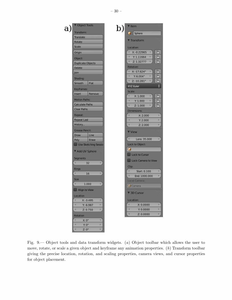
Rotating the data cube. We can keyframe the initial state by pressing the Insert Keyframe

button on the Object Tools panel (Figure 9) and choosing the option Rotation, which locks the

rotation of the mesh cube for that particular frame. The cube can be rotated about the z -axis

(blue) by moving the green marker on the animation timeline to frame 300 (halfway through the

planned animation) and changing the z -rotation (right hand transformation toolbar) to 180

degrees and again choosing Insert Keyframe, Rotation. This is repeated a third and final time

for frame 600, with the z -rotation to 360 degrees. The play button can then be engaged on the

bottom animation toolbar and a preview of the animation motion will be shown.

– 13 –

Revolving the camera. In this example we keep the cube mesh object stationary and move

the camera along a path. This can be accomplished by choosing the Add, Curve, Circle at the

top of the main interface (see Figure 1) and scaling it (s key) to the size of the path needed to

view the data cube. The path animation can be keyframed under the Object Data tab just like

any other object in Blender, rotating the path 360 degrees (or more) during the course of our 600

frame, 20 s output. The camera can then be constrained with a Follow Path constraint with its

local y-axis normal to the circle, and further constrained with a Track To control with the z -axis

of the camera normal to the focal plane pointing to the data cube (Figure 12).

4.4. Rendering and Output

Once the data cube, tracking paths, and camera have been keyframed, the output can be ren-

dered. Under the render tab there are two options: Render and Animation. Render will allow

the user to view the output of the current frame as viewed in the animation timeline. Animation

will render out all the frames of the current scene. Most of the default parameters will work well for

typical visualization scenarios. We recommend checking the Stamp box which will place metadata

about the animation on each image, including parameters used in the animation settings. Output

can be specified as still images for each frame or one of several video outputs. The setup and a

rendered frame from the final output is depicted in Figure 15.

5. Example Visualizations

In addition to the data cube example highlighted in section 4, we outline a number of other

astronomical visualizations that are likely of use to the community. Blender has found successful use

in materials science, medicine, biology, fluid dynamics, and network theory (Norman 2012; Cazotto

et al. 2013; Andrei et al. 2012; Rana & Herrmann 2011; Valverde & Sole 2005). In the case of

studying large scale structure, Blender provided an interface for examining redshift distortions and

correlations between quasar absorption line systems and luminous red galaxies (SubbaRao et al.

2008). Results from these kinds of studies are extremely challenging to discern with two-dimensional

plots. As larger catalogs with expanded parameter sets begin to become the norm rather than the

exception, having a 3D graphics and rendering environment like Blender for astronomers will prove

to be an invaluable tool. We provide the following examples to illustrate starting points for those

interested in pursuing their own visualization scenarios for both exploratory research as well as

outreach endeavors. The visualizations are designed to put into practice aspects of the interface

described in section 3. Example data, files, and tutorials will be provided for download in section

6.

– 14 –

5.1. Astronomical Catalog

We can use a small sample of galaxy distances to illustrate the mapping and animating of a

catalog fly-through. Figure 16 shows a Blender scene setup and a single frame render of data from

the Extragalactic Distance Database (EDD12; Tully et al. 2009) of galaxies in the nearby Universe

(cz⊙ < 3000 km s−1).

This example can utilized in scientific data exploration because we can examine the overall

structure of the catalog in real time with the 3D view space. Since each galaxy has a unique object

identifier in the data structure, we can use the Blender search function (Spacebar) and period key

(.) to immediately center and zoom to any galaxy. This is useful for research, but also for planning

camera movements for rendering if so desired.

Importing and rendering an astronomical catalog makes use of the simplest type of mesh -

a vertex point, Python scripting, texturing, animation, camera movement, and rendering. ASCII

catalogs can be read into Python lists. A template object can be created with a single vertex

textured with a halo in the Materials tab, size set to 0.020. Under the Textures tab, the Type

should be set to ”Blend.” The camera can then be keyframed for animation.

5.2. N -body Simulation

This example of a galaxy simulation was generated with GADGET-2 (Springel 2005). Each

large spiral disk galaxy has 10000 disk particles and 20000 halo particles with Milky Way scale

lengths and masses. The simulation is run for approximately 1100 timesteps for a total simulation

runtime of 2 billion yr. We read in the particle x, y, z coordinates as single vertex with a small

Gaussian halo as its materials texture. The snapshot file for each time step is keyframed as one

frame in the animation. In addition, a Bezier curve can be added to the scene as an object path

(Farouki 2012). The camera can then be flown along the curve as the galaxy interaction progresses

(Figure 17).

Blender has excellent utility for research purposes in rendering simulations. Many simple as-

tronomical simulations are of the format x-y-z over time and are easily accommodated. The camera

control in particular is useful for moving through 3D space as simulation timesteps play through

an animated rendering. The procedure is very similar to opening a catalog in the previous exam-

ple; for a simulation we can open different snapshots and keyframe to create a smooth animation.

Snapshot files can be read into a Python list or dictionary. A template object can be created with

a single vertex textured with a halo in the Materials tab, size set to 0.020. Under the Textures

tab, the Type should be set to ”Blend.” The positions of each particle can then be loaded with the

Python API. The camera can be keyframed for animation and a final rendering can be generated.

12Data available at http://edd.ifa.hawaii.edu/

– 15 –

5.3. Asteroid Models

We show a number of 3D asteroid models based on data available from the Database for

Asteroid Models from Inversion Techniques (Durech et al. 2010). The database provides Wavefront

object files of each asteroid model, which can easily be loaded into the 3D viewport. For this

example, we want uniform lighting to be able to see the entire surface model as they are rotated.

This can be accomplished by turning on Environment Lighting in the World tab (small globe icon,

see Figure 12). Figure 18 exhibits an example of an orthographic projection and shows a sample

of six asteroids, enlarged to show the smoothing texture on the surfaces.

This example exhibits how 3D mesh models in OBJ files can be imported into Blender for

animation and rendering. OBJ files from data such as our asteroid example can be used for research

purposes, but also have merit in video renderings for public outreach. This can be accomplished

in the upper left corner of the GUI and choosing File, Import, Wavefront (*.obj). The object can

be scaled in the Transform dialog on the right side of the GUI, or by pressing the ’S’ key. The

asteroid mesh object can be selected with the right mouse button, keyframed for animation with

the ”I” key, and rotated with the ”R” key.

6. Summary

The availability of hardware and software that allows the creation of high-quality 3D ani-

mations for astronomy brings a vivid new way for astronomers to visualize and present scientific

results. Animations are an important part of the astronomical toolset that can show expanded

phase spaces, the time domain, or multidimensional tables and catalogs beyond the limitations

posed by two-dimensional plots and images.

An introduction has been presented showing the software program Blender as a 3D anima-

tion and rendering package for astronomical visualization. We have reviewed the importance of

visualization in the scientific disciplines, with examples from astronomy. Features of the program

include GPU processing, a variety of rendering engines, and an API for scripting. An overview

of the principles in the animation workflow include modeling, volumetric and surface texturing,

lighting, animation, camera work, rendering, and compositing. With these general steps in mind

various astronomical datasets – images, data cubes, and catalogs can be imported and visualized.

An example workflow session with an astronomical data cube that shows the structure and

dynamics of a small dwarf galaxy has been presented, giving settings and recommendations volu-

metric texturing of a cube model, animation, and animation output. A number of other example

are shown from different areas of astronomy to give a broad scope of possibilities that might exist

with astronomical data.

A demonstration video as well as Blender files, Python scripts, and basic tutorials of the

principles and examples outline in this paper are available at:

– 16 –

http://www.cv.nrao.edu/∼bkent/computing/kentPASP.html

REFERENCES

Ament, M., Weiskopf, D., & Carr, H. 2010, IEEE Trans. Visual. Comput. Graph., 16, 1505

Andrei, R. M., Callieri, M., Zini, M., Loni, T., Maraziti, G., Pan, M., & Zoppe, M. 2012, BMC

Bioinf., 13(Suppl 4), S16

Autin, L., Johnson, G., Hake, J., Olson, A., & Sanner, M. 2012, IEEE Comput. Graph. Appl., 32,

50

Balakrishnan, R., & Kurtenbach, G. 1999, in Proc. of the SIGCHI Conf. on Human Factors in

Computing Systems (New York: ACM), 56

Barrett, P. E., & Bridgman, W. T. 2000, in ASP Conf. Ser. 216, Astronomical Data Analysis

Software and Systems IX, ed. N. Manset, C. Veillet, & D. Crabtree (San Francisco: ASP),

67

Bate, N. F., Fluke, C. J., Barsdell, B. R., Garsden, H., & Lewis, G. F. 2010, NewA, 15, 726

Bergeron, R. D., & Foulks, A. 2006, in ASP Conf. Ser. 359, Numerical Modeling of Space Plasma

Flows, ed. G. P. Zank & N. V. Pogorelov (San Francisco: ASP), 285

Bertin, E., & Arnouts, S. 1996, A&AS, 117, 393

Birn, J. 2000, Digital Lighting and Rendering (second ed.; Thousand Oaks: New Riders)

Blinn, J. F. 1978, SIGGRAPH Comput. Graph., 12, 286

Boch, T., Oberto, A., Fernique, P., & Bonnarel, F. 2011, in ASP Conf. Ser. 442, Astronomical Data

Analysis Software and Systems XX, ed. I. N. Evans, A. Accomazzi, D. J. Mink, & A. H.

Rots (San Francisco: ASP), 683

Borkin, M., Goodman, A., Halle, M., & Alan, D. 2007, in ASP Conf. Ser. 376, Astronomical Data

Analysis Software and Systems XVI, ed. R. A. Shaw, F. Hill, & D. J. Bell (San Francisco:

ASP), 621

Brinkmann, R. 2008, The Art and Science of Digital Compositing: Techniques for Visual Effects,

Animation and Motion Graphics (second ed.; Burlington: Morgan Kaufmann)

Buddelmeijer, H., & Valentijn, E. 2013, Exp. Astron., 35, 283

Carlbom, I., & Paciorek, J. 1978, ACM Comput. Surv., 10, 465

Cazotto, J. A., Neves, L. A., Machado, J. M., et al. 2013, Journal of Physics Conference Series,

410, 012169

– 17 –

Comparato, M., Becciani, U., Costa, A., Larsson, B., Garilli, B., Gheller, C., & Taylor, J. 2007,

PASP, 119, 898

Crassin, C., Neyret, F., Lefebvre, S., Eisemann, E. 2009, in Proc. 2009 Symp. on Interactive 3D

Graphics and Games (New York: ACM), 15

Debevec, P. 1998, in Proc. twenty-fifth Annual Conference on Computer Graphics and Interactive

Techniques (New York: ACM), 189

Diehl, S. 2007, Software Visualization: Visualizing the Structure, Behaviour, and Evolution of

Software (Heidelberg: Springer-Verlag)

Draper, P. W., Berry, D. S., Jenness, T., Economou, F., & Currie, M. J. 2008, in ASP Conf.

Ser. 394, Astronomical Data Analysis Software and Systems XVII, ed. R. W. Argyle, P. S.

Bunclark, & J. R. Lewis (San Francisco: ASP), 339

Drebin, R. A., Carpenter, L., & Hanrahan, P. 1988, SIGGRAPH Comput. Graph., 22, 65

Duff, T., 1985, SIGGRAPH Comput. Graph., 41

Durech, J., Sidorin, V., & Kaasalainen, M. 2010, A&A, 513, A46

Elvidge, C. D., Baugh, K., E., Kihn, E. A., Kroehl, H. W., & Davis, E. R. 1997, Photogramm.

Eng. Remote Sensing, 63, 727

Elvins, T. T. 1992, SIGGRAPH Comput. Graph., 26, 194

Farouki, R. T. 2012, Comput. Aided Geom. Des., 29, 379

Feng, Y., Croft, R. A. C., Di Matteo, T., et al. 2011, ApJS, 197, 18

Frenkel, K. A. 1988, Commun. ACM, 31, 111

Friendly, M. 2006, in Handbook of Computational Statistics: Data Visualization, Vol. III ed.

C. Chen, W. Hardle, & A. Unwin (Heidelberg: Springer-Verlag), 1

Garland, M., Le Grand, S., Nickolls, J., et al. 2008, IEEE Micro, 28, 13

Gooch, R., 1995, in Proc. sixth Conference on Visualization (Washington, DC: IEEE Computer

Society), 374

Goodman, A. A. 2012, Astron. Nachr., 333, 505

Hansen, C. D., & Johnson, C. R. eds. 2005, The Visualization Handbook (San Diedo: Academic

Press)

Hassan, A., & Fluke, C. J. 2011, Proc. Astron. Soc. Australia, 28, 150

Hassan, A. H., Fluke, C. J., & Barnes, D. G. 2012, Proc. Astron. Soc. Australia, 29, 340

– 18 –

Hess, R. 2010, Blender Foundations: The Essential Guide to Learning Blender 2.6. (Burlington:

Focal Press)

Hunter, J. 2007, Comput. Sci. Eng., 9, 90

Jacob, J. C., & Plesea, L. 2001, in Proc. IEEE Aerospace Conf., Vol. 7, 7–3530

Kent, B. R. 2011, in ASP Conf. Ser. 442, Astronomical Data Analysis Software and Systems XX,

ed. I. N. Evans, A. Accomazzi, D. J. Mink, & A. H. Rots (San Francisco: ASP), 625

Kuchelmeister, D., Muller, T., Ament, M., Wunner, G., & Weiskopf, D. 2012, Comput. Phys.

Commun., 183, 2282

Laramee, R. S. 2008, Softw. Pract. Exp., 38, 735

Leech, J., & Jenness, T. J. 2005, in ASP Conf. Ser. 347, Astronomical Data Analysis Software and

Systems XIV, ed. P. Shopbell, M. Britton, & R. Ebert (San Francisco: ASP), 143

Levay, Z. 2011, in ASP Conf. Ser. 442, Astronomical Data Analysis Software and Systems XX, ed.

I. N. Evans, A. Accomazzi, D. J. Mink, & A. H. Rots (San Francisco: ASP), 169

Levoy, M. 1988, IEEE Comput. Graph. Appl., 8, 29

Lipsa, D. R., Laramee, R. S., Cox, S. J., Roberts, J. C., Walker, R., Borkin, M. A., & Pfister, H.

2012, Comput. Graph. Forum, 31, 2317

Lorensen, W. E., & Cline, H. E. 1987, SIGGRAPH Comput. Graph., 21, 163

Lupton, R., Blanton, M. R., Fekete, G., Hogg, D. W., O’Mullane, W., Szalay, A., & Wherry, N.

2004, PASP, 116, 133

Mercer, R. A., & Klimenko, S. 2008, Class. Quantum Gravity, 25, 184025

Molnar, S., Cox, M., Ellsworth, D., & Fuchs, H. 1994, Comput. Graph. Appl., 14, 23

Moloney, B., Ament, M., Weiskopf, D., & Moller, T. 2011, IEEE Trans. Visual. Comput. Graph.,

17, 1164

Munzner, T., Johnson, C., Moorhead, R., Pfister, H., Rheingans, P., & Yoo, T. S. 2006, IEEE

Comput. Graph. Appl., 26, 20

Murray, J. D., & van Ryper, W. 1996, Encyclopedia of Graphics File Formats (second ed.) (Paris:

O’Reilly & Associates, Inc.)

Norman, C. 2012, Science, 335, 525

Patoli, M., Gkion, M., Al-Barakati, A., Zhang, W., Newbury, P., & White, M. 2009, in IEEE Power

Systems Conference and Exposition (Seattle: IEEE), 1

– 19 –

Peng, H., Ruan, Z., Long, F., Simpson, J. H., & Myers, E. W. 2010, Nat. Biotechnol., 28, 348

Phong, B. 1975, Commun. ACM, 18, 311

Porter, T., & Duff, T. 1984, SIGGRAPH Comput. Graph., 18, 253

Price, R., Puchala, J., Rovito, T., & Priddy, K. 2011, in Proc. IEEE National Aerospace and

Electronics Conf. (Fairborn: IEEE), 291

Rana, S., & Herrmann, M. 2011, Phys. Fluids, 23, 091109

Rector, T. A., Levay, Z. G., Frattare, L. M., English, J., & Pu’uohau-Pummill, K. 2007, AJ, 133,

598

Reniers, D. & Telea, A., 2008, in IEEE International Conf. on Shape Modeling and Applications

(Stony Brook: IEEE), 273

Rhyne, T.-M. 2012, in ACM SIGGRAPH 2012 Courses (New York: ACM), 1:1–1:82

Robinson, A. H. 1982, Early Thematic Mapping in the History of Cartography (Chicago: University

of Chicago Press)

Scianna, A. 2013, Appl. Geomatics, 1

Shahidi, R., Lorensen, B., Kikinis, R., Flynn, J., Kaufman, A., & Napel, S. 1996, in Proc. seventh

IEEE Conf. on Visualization (San Francisco: IEEE), 439

Springel, V. 2005, MNRAS, 364, 1105

Staples, M. L., & Bieman, J. M. 1999, Adv. Comput., 49, 95

Stone, J., Gohara, D., & Shi, G. 2010, Comput. Sci. Eng., 12, 66

Strand, R., & Borgefors, G. 2005, Comput. Vision Image Understand., 100, 3

Strehl, A., & Ghosh, J. 2002, INFORMS J. Comput., 15, 2003

SubbaRao, M. U., Aragon-Calvo, M. A., Chen, H. W., Quashnock, J. M., Szalay, A. S., & York,

D. G. 2008, New J. of Phys., 10, 125015

Taylor, R., Davies, J. I., & Minchin, R. F. 2011, in AAS Meeting Abstracts 218, 408.22

Teuben, P. J., Hut, P., Levy, S., Makino, J., McMillan, S., Portegies Zwart, S., Shara, M., &

Emmart, C. 2001, in ASP Conf. Ser. 238, Astronomical Data Analysis Software and Systems

X, ed. F. R. Harnden, Jr., F. A. Primini, & H. E. Payne (San Francisco: ASP), 499

Teyseyre, A. R., & Campo, M. R. 2009, IEEE Trans. Visual. Comput. Graph., 15, 87

– 20 –

Tully, R. B., Rizzi, L., Shaya, E. J., Courtois, H. M., Makarov, D. I., & Jacobs, B. A. 2009, AJ,

138, 323

Turk, M. J., Smith, B. D., Oishi, J. S., Skory, S., Skillman, S. W., Abel, T., & Norman, M. L.

2011, ApJS, 192, 9

Valverde, S., & Sole, R. V. 2005, Phys. Rev. E, 72, 026107

Wainer, H., & Velleman, P. F. 2001, Ann. Rev. Psychol., 52, 305

Wallace, G. K. 1991, Commun. ACM, 34, 30

Walter, F., Brinks, E., de Blok, W. J. G., Bigiel, F., Kennicutt, R. C., Jr., Thornley, M. D., &

Leroy, A. 2008, AJ, 136, 2563

Wenger, S., Ament, M., Guthe, S., Lorenz, D., Tillmamm, A., Weiskopf, D., & Magnor, M. 2012,

IEEE Trans. Visual. Comput. Graph., 18, 2188

Yagel, R. 1996, SIGGRAPH Tutorial Notes, Course No. 34 (New Orleans: ACM)

Yost, B., & North, C. 2006, IEEE Trans. Visual. Comput. Graph., 12, 837

Zini, M. F., Porozov, Y., Andrei, R. M., Loni, T., Caudai, C., & Zoppe, M. 2010, preprint

(arXiv:1009.4801)

This preprint was prepared with the AAS LATEX macros v5.2.

– 21 –

Table 1. Blender Data Formats

Format Type Suffix Usage

Blend native .blend Import/Export

OBJ ASCII .obj Import/Export

CSV ASCII .csv Importa

JPEG image .jpg, .jpeg Importb / Export

TIF image .tif, .tiff Importb / Export

PNG image .png Importb / Export

GIF image .gif Importb / Export

EXR image .exr Import

FITS image/structured data .fit, .fits Importa

AVI video .avi Export

MPEG video .mpg, .mpeg Export

MOV video .mov Exportc

H.264 video .mov Exportc

Note. — We provide examples and scripts in Section 6.

aCan be imported via standard Python file I/O.

bCan be used for surface mesh texturing.

cCan be achieved on Linux-based OS via FFmpeg

(http://www.ffmpeg.org)

Table 2. Rendering Time Benchmark Comparison

Render Samples Mean Median SEx

N minutes minutes

NVidia CUDA 100 2.82 1.49 0.31

OpenCL 31 2.17 1.99 0.22

CPU 154 8.30 6.48 0.47

Note. — Rendering time for a Blender session in the

Cycles engine at a resolution of 960 × 540 pixels with

rendering tile sizes of 8 × 8 pixels. The benchmark test

consisted of 6 camera views and 12 mesh objects total-

ing 86,391 polygons and 91,452 vertices. The last column

describes the standard error of the mean.

– 22 –

Table 3. Comparison of 3D Graphics Software and Engines

Format Platforma License/Avail Featuresb Free?c Reference

Blender L,M,W GPL MM, A, T, iR, eR, L, S, VE, N Yes 1

3D Studio Max W Proprietary MM, A, T, iR, eR(some), L No 2

Cinema 4D L,M,W Proprietary MM, A, T, L, eR No 3

EIAS3D M,W Proprietary MM, A, T, L, iR No 4

Houdini L,M,W Proprietary MM, A, T, L, eR No 5

Lightwave 3D M,W Proprietary MM, A, T, L, iR No 6

Maya L,M,W Proprietary MM, A, T, L, iR, No 7

Modo M,W Proprietary MM, A, T, L No 8

SAP V.E.S. W Propreitary MM, A, iR No 9

SoftImage L,W Propreitary MM, A, S, N No 10

Note. — References and Vendor websites:

(1) http://www.blender.org/

(2) http://www.autodesk.com/products/autodesk-3ds-max/overview/

(3) http://www.maxon.net/

(4) http://www.eias3d.com/

(5) http://www.sidefx.com/

(6) https://www.lightwave3d.com/

(7) http://www.autodesk.com/products/autodesk-maya/overview/

(8) http://www.luxology.com/modo/

(9) Visual Enterprise Solutions

including Client View and Deep Server: http://www.sap.com/

(10) http://www.autodesk.com/products/autodesk-softimage/overview/aM: Mac OS X, L: Linux, W: Windows

bMM: 3D Mesh models, A: animation control, T: 2D/3D texture mapping, iR: internal rendering, eR: support

for external rendering, L: lighting control, S: 3D sculpting, VE: video editing, N: Node editing

cSome commercial software vendors offer free trials.

– 23 –

Fig. 1.— Main Blender interface. (a) Object Toolbar for manipulating a selected object. (b) Main

3D view port. In this example a ”Quad View” is shown for the top, front, and right orthographic

perspectives, as well as the preview of the camera angle. (c) Transformation toolbar which allows

precise control of objects. (d) Hierarchical data outliner, summarizing the properties and settings

of each data structure. (e) Properties panel for the camera, world scene environment, constraints,

materials, and textures. (f ) Animation time line, frames in the video animation, and yellow marks

indicating keyframes for selected objects.

– 24 –

Fig. 2.— Six basic mesh primitives. This example scene shows faceted versions of a cube, UV-

sphere, icosahedron, cylinder, cone, and torus, each colored with a different material. These are

simple objects upon which more complex models can be built.

Fig. 3.— Three different control handlers of the interface. Red, blue, and green controls correspond

to x, y, and z. (a) Translation widget arrows, (b) Meridians of the rotation widget. (c) Box handlers

of the scaling widget.

– 25 –

Fig. 4.— Example of UV mapping with data from the Defense Meteorological Satellite Program

(DMSP) Operational Linescan System (OLS; Elvidge et al. 1997), shown in (a). The surface of the

UV-sphere is mapped onto the cylindrical projection of the nighttime view of the Earth in (b); (c)

shows the final result of the mapping.

– 26 –

Fig. 5.— Example graph editor session that allows the user to manipulate complex movement

curves. A camera with red, blue and green curves for its x, y, and z location is shown as it tracks an

object in a circular orbit. The representation shown here moved the camera closer to the object at

periapsis and then passes through the orbital plane. The thin orange lines tangent to the curves act

as control handles for manipulation. The horizontal axis shows the frame number and the vertical

axis shows the position along the respective x,y, or z -axis.

– 27 –

Fig. 6.— Blender workflow process. (a) UV-sphere mesh. (b) Model with Mars data uv -mapped

onto the mesh. (c) Lighting element being applied. (d) Small curve with the lighting element

being animated. (e) Camera animation curve (lower left in the panel) with a Track To constraint

applied in the Properties panel. This allows the camera to move along the path but to always be

focused on the mesh sphere. (f ) Frame of the final render and composite.

– 28 –

Fig. 7.— Data object structures and flow in Blender. Model, lighting, lamera, and animation

properties are fed into different render layers. These render layers are then composited into a

final video or still frame, with compositing indicated by⊗

. In this example, each render layer is

captured by cameras, but models only contribute to the first layer shown on the top. Other layers

might include backgrounds, lighting, blurs, or lens flares that are composited after the models are

rendered and textured.

– 29 –

Fig. 8.— Benchmark comparison running a Blender session in Cycles at a resolution of 960 × 540

pixels with rendering tile sizes of 8 × 8 pixels. The distribution of render times shown are for

NVidia CUDA (solid blue line), and OpenCL (dotted green line), and CPU processing (dashed red

line), each binned in 1 minute intervals. The vast majority of GPU runs with CUDA and OpenCL

outperform standard CPU-based rendering.

– 30 –

Fig. 9.— Object tools and data transform widgets. (a) Object toolbar which allows the user to

move, rotate, or scale a given object and keyframe any animation properties. (b) Transform toolbar

giving the precise location, rotation, and scaling properties, camera views, and cursor properties

for object placement.

– 31 –

Fig. 10.— Data outliner widget. This hierarchical tree view depicts the program’s outline of all

objects within the scene. In this example, the Camera has a ”Track To” constraint applied. The

map has a simple lighting texture, and the sphere (a planet in this case) has a material and UV-

mapped texture applied. Each object is displayed in the view port, indicated by the eye icon. Each

object is also applied to at least one render layer, indicated by the camera icon on the right hand

side.

– 32 –

Fig. 11.— Tab icons at top highlight the material and texture widgets. (a) Material widget gives

the user the options to modify lighting, specular, and shading parameters, and whether what kind

of material (surface, wire, volume, or halo) will be applied to the object. (b, c) Texture widget for

applying surface and volume textures, as well as color maps, to the objects.

– 33 –

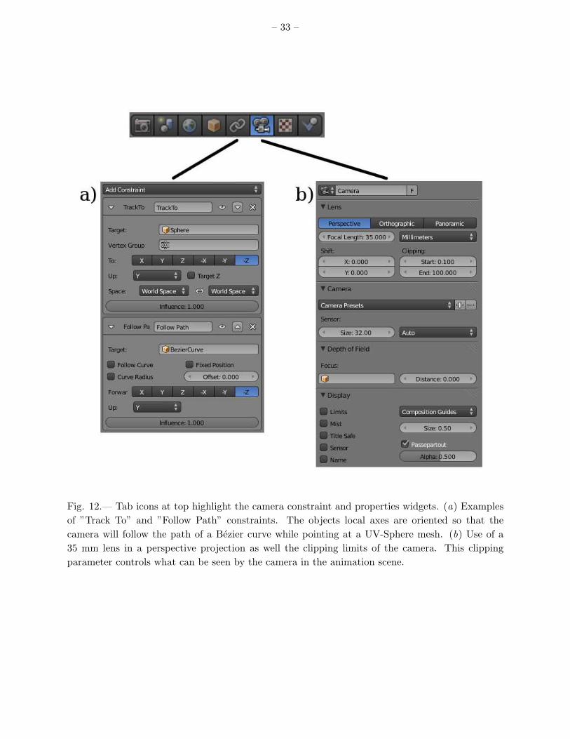
Fig. 12.— Tab icons at top highlight the camera constraint and properties widgets. (a) Examples

of ”Track To” and ”Follow Path” constraints. The objects local axes are oriented so that the

camera will follow the path of a Bezier curve while pointing at a UV-Sphere mesh. (b) Use of a

35 mm lens in a perspective projection as well the clipping limits of the camera. This clipping

parameter controls what can be seen by the camera in the animation scene.

– 34 –

Fig. 13.— Differences between (a) perspective and (b) orthographic projection. Each view has

applications in astronomical visualization.

– 35 –

Fig. 14.— Multiple camera angles are shown, with vectors pointing at an Earth surface mesh that

are normal to the film planes (yellow crosses). The camera in the lower left of the top panel is

following a Bezier curve path while tracking the planet model. The lower panel shows a perspective

projection through the camera view.

– 36 –

Fig. 15.— Top: View space setup for a data cube and camera in an orthographic projection.

Bottom: Final perspective projection rendering of an H I data cube.

– 37 –

Fig. 16.— Three-dimensional view of a nearby galaxy catalog (cz⊙ < 3000 km s−1) from the

Extragalactic Distance Database (EDD). (a, b, c) Front, right, and top orthographic projections,

respectively. (d) Single render frame from the animation in a perspective projection.

– 38 –

Fig. 17.— Three-dimensional view of a simulation with colliding galaxies. (a, b, c) Front, right,

and top orthographic projections, respectively. (d) Single render frame from the animation in a

perspective projection.

– 39 –

Fig. 18.— Asteroid models in this figure show how OBJ files can be rendered in Blender. The

models are not shown to relative scale and have been increased in size for detail.