vlsi implementation of spatial modulation mimo system...

International Journal of Engineering Technology, Management and Applied Sciences

www.ijetmas.com December 2014, Volume 2 Issue 7, ISSN 2349-4476

196 Mohammad Irshad Begum, Dr. Pushpa Kotipalli

VLSI Implementation of Spatial Modulation MIMO System

for Wireless communication Networks

Mohammad Irshad begum Dr. Pushpa Kotipalli

M.Tech.,(VLSID) Student Professor: ECE Department, Head of ATL

Shri Vishnu Engineering College for Women Shri Vishnu Engineering College For Women

Bhimavaram, Andhra Pradesh, India Bhimavaram, Andhra Pradesh , India

Abstract-- MIMO (Multiple Input Multiple Output) is

an antenna technology for wireless communications in

which multiple antennas are used at both the source and

destination to send multiple parallel signals. Spatial

Modulation (SM) is a transmission technique proposed

MIMO systems, where only one transmit antenna is

active at a time. In SM, information bits are conveyed

through the index of the active transmit antenna in

addition to the information bits conveyed through

conventional modulation symbols. In spatial

modulation, the stream of bits to be transmitted in one

channel is divided into two groups. One group i.e., m-

bit sequence chooses one antenna from a total of Nt =

2m antennas. A known signal is transmitted on this

chosen antenna. The remaining Nt -1 antennas remain

silent. The second group determines the symbol to be

transmitted from the chosen antenna.

In this paper we present the VLSI implementation of

Spatial Modulation MIMO system. The active antenna

number detection algorithm called Iterative Maximal

Ratio Combining (i-MRC) algorithm is presented This

system is designed in VHDL language, simulated using

Modelsim simulator and realized on SPARTRAN-3E

FPGA Kit. Experimental results of the proposed

technique shows the increased performance in terms of

Accuracy.

Index Terms – Spatial Modulation (SM), Multiple-

input- Multiple- output (MIMO), Interchannel

interference (ICI), Receiver Complexity. IEE-754

Single precision Floating point format.

1. INTRODUCTION MIMO transmits and receives two or more data streams

through a single radio channel. Thereby the system can

deliver two or more times the data rate per channel

without additional bandwidth or transmit power. The

need to improve the spectral efficiency and reliability of

radio communication is driven by the ever increasing

requirement for higher data rates and improved Quality

of service (QOS) across wireless links. MIMO

technology is one solution to attain this by transmitting

multiple data streams from multiple antennas. MIMO

transmission strongly depends on transmit and receive

antenna spacing, transmit antenna synchronization and

the reduction of interchannel interference (ICI) at the

receiver input. An alternative transmission approach

that entirely avoids ICI at the receiver input is used for

BPSK and QPSK transmission respectively. The basic

idea is to compress a block of Nt symbols into a single

symbol prior to transmission, where Nt indicates the

number of transmit antennas. Information is retained by

this

symbol and is mapped to one and only one of the Nt

antennas. The task of the receiver is twofold: First, to

estimate the single symbol and second to detect the

respective antenna number from which the symbol is

transmitted. However this scheme suffers from a loss of

Spectral efficiency. Traditional modulation techniques

such as BPSK (binary phase shift keying), QPSK

(Quadrature phase shift keying) etc. map a fixed

number of information bits into one symbol. Each

symbol represents a constellation point in the complex

two dimensional signal planes. This is referred to as

signal modulation. In this paper an alternative

transmission approach is proposed in which this two

dimensional plane is extended to a third dimension i.e.,

spatial dimension. This is referred as Spatial

modulation. This new transmission technique will result

in a very flexible mechanism which is able to achieve

high spectral efficiency and very low receiver

complexity. SM is a pragmatic approach for

transmitting information, where the modulator uses well

known modulation techniques (e.g., QPSK, BPSK), but

also employs the antenna Index to convey information.

Ideally, only one antenna remains active during

transmission so that ICI is avoided. Spatial Modulation

(SM) is a recently proposed spatial multiplexing

scheme for Multiple-Input-Multiple-Output (MIMO)

systems without requiring extra bandwidth or extra

transmission power. SM does not place any restriction

on the minimum number of receive-antennas. This is

particularly beneficial for mobile handsets because of

the limited available space and the cost constraints for

these mass market devices. All these properties and

requirements make SM a very attractive MIMO scheme

for many potential applications. The idea of using the

transmit antenna number as an additional source of

information is utilized in spatial modulation. The

number of information bits that can be transmitted using

http://www.ijetmas.com/




spatial modulation depends on the used constellation

diagram and the given number of transmit antennas.

II. SYSTEM MODEL This paper is organized as follows: In section II System

model is discussed, in section III hardware

implementation is discussed, section IV is simulation

results and section V is conclusion.

We consider a generic Nt × Nr Multiple-Input-

Multiple-output (MIMO) system with Nt and Nr being

the number of transmit and receive antennas

respectively. Moreover, we assume that the transmitter

can send digital information via M distinct signal

waveforms (i.e., the so-called signal-constellation).

Fig.1. MIMO Network with Nt Transmit antennas and Nr

Receive antennas

Each spatial constellation point defines an independent

complex plane of signal constellation points.

1. A symbol is chosen from a complex signal

constellation diagram.

2. A unique transmit antenna index is chosen

from the set transmit antennas in the antenna

array.

The principal working mechanism of spatial modulation

is depicted in Fig:2. For illustrative purposes only two

of such planes are shown in Fig.2. For i) Nt = 4 and ii)

M = 4.

Legend: i) Re = real axis of the signal constellation

diagram and

ii) Im = imaginary axis of the signal

constellation diagram.

In Fig.2 the information bits are grouped into four bits.

The left group indicates the antenna index and the right

group indicates the information bits to be transmitted

based on the used modulation technique.

Fig.2. Illustration of the 3-D encoding of Spatial

Modulation.

The spatial modulation system model is shown in Fig 3.

q (k) is a vector of n bits to be transmitted. The binary

vector is mapped into another vector x(k). Symbol

number l in the resulting vector x(k) is xl , where l is the

mapped transmit antenna number l € [1:Nt]. The

symbol xl is transmitted from the antenna number l over

the MIMO channel, H(k). H(k) can be written as a set

of vectors where each vector corresponds to the channel

path gains between transmit antenna v and the receive

antennas as follows:

H = [h1 h2 h3 ….. h Nt] (1)

Where:

hv = [h1,v h2,v … hNr,v]T

(2)

Similarly for a Nt x Nr MIMO system the channel

matrix is given as

H (k) is the Nt x Nr discrete time invariant frequency

response channel matrix. The received vector y(k) is

given as

y(k) = H(k)xl +w(k) (3)

where w(k) is the Additive White Gaussian noise

vector. The received vector y(k) is obtained as follows

y1 = h11x1+h12x2+h13x3+….+h1Nx4

y2= h21x1+h22x2+h33x3+… +h2Nx4

y3= h31x1+h32x3+h33x3 +….+h3Nx4

…. ……. ….. …. …… ….. ……

yM= HM1x1+hM2x2+HM3x3+….hMNxN





Fig.3: Spatial Modulation system model

The number of transmitted information bits n, can be

adjusted in two different and independent ways either

by changing the signal modulation and/or changing the

spatial modulation. Different modulation techniques can

be used for SM-MIMO such as BPSK, QPSK, 8QAM,

16QAM, 32QAM etc. These modulation techniques

will be used to map the information bits to the symbols

by using constellation diagrams. For example we

consider only BPSK and QPSK modulation techniques.

Table 1: Symbol mapping table for BPSK and QPSK

Modulation techniques.

The transmitter of the SM-MIMO system has to

transmit the symbol and also have to select the antenna

for the transmission of the symbol from the group of

antennas. A block of information bits is mapped into the

constellation point in the signal and spatial (antenna)

domain. From the binary source the serially generated

binary data will be converted to parallel data. This

binary data will be segmented into two groups

containing log2(Nt)+log2(M) bits each with log2(Nt) and

log2(M) being the number of bits needed to identify a

transmit antenna in the antenna-array and a symbol in

the signal constellation diagram respectively.

Fig.4. Spatial Modulation Mapper.

The bits in the first sub-block are used to select the

antenna that is switched on for data transmission, while

all other transmit antennas are kept silent in the current

signaling time interval. The bits in the second sub-

block are used to choose a symbol in the signal

constellation diagram using SM mapper [4] as shown in

Fig:4. In general the number of bits that can be

transmitted using spatial modulation is given as follows

n = log2 (Nt) +m (4)

Where

m = log2 (M) (5)

Where ‘M’ is the used constellation size





Fig.5. 3bits Transmission using BPSK and four transmit antennas and QPSK using two transmit antennas

The transmission of binary data using spatial

modulation is carried out over a Wireless Rayleigh Flat

Fading Channel. The channel is a complex NtxNr

Matrix. ‘Nt’ denotes the number of transmitting

antennas and ‘Nr’ denotes the receiving antennas. It

contains the channel path gains between N transmit and

M receive antennas. The channel varies based on the

number of transmit antennas and the used signal

modulation.

III.HARDWARE IMPLEMENTATION OF

SM-MIMO SYSTEM

a) Spatial Modulation Transmitter

The SM-MIMO transmitter has to perform two tasks of

choosing the active antenna index and binary data has

to be transmitted from that active antenna which is

made active for the purpose of transmission as shown in

Fig.6.

Fig.6. Spatial Modulation Transmitter

The SM-MIMO transmitter is implemented in the

hardware using N-bit register to store the N bits of

binary data. This serial data is converted to parallel by

the serial to parallel converter. As the number of bits

transmitted using SM depends on the used constellation

size, for BPSK and QPSK we can transmit 3bits at a

particular time instant. The transmitter using BPSK

modulation is shown in Fig.7.

Fig.7. SM Transmitter using BPSK and 4 Antennas.

As shown in Fig.7 the 2 to 4 decoder is used to decode

the antenna index bits into four indicating which

antenna is made active for transmission based on the

incoming bit stream. BPSK requires two bits to indicate

antenna index and one bit to represent symbol.

Fig.8. SM Transmitter using QPSK and 2 Antennas.





The transmitter using QPSK modulation requires two

bits to represent the modulated symbol and one bit to

indicate the antenna index. Hence it requires only two

transmit antennas as shown in Fig.8. Here 1 to 2

decoder is used to decode the active antenna which is

set for transmission. The transmission gates are used as

switches which is made ON/OFF based on the decoder

output.

b) Spatial Modulation Receiver

The Receiver of the SM-MIMO system is assumed to

have full knowledge of the channel through which the

transmission took place. The channel is a complex

matrix consisting of complex elements consisting of

both real and imaginary parts. These complex fractional

numbers are finally converted to binary bits by using

the IEEE-754 floating point format. The Receiver

performs the complex multiplications and complex

additions between the channel matrix H(k) and received

vector y(k).

The receiver chooses the transmit antenna number

which gives highest correlation. The task of the receiver

is twofold:

i) To estimate the transmitted symbol

and

ii) To detect the respective antenna

number from which the symbol is

transmitted.

Fig.9. Spatial Modulation Receiver

Assume the following sequence of bits to be

transmitted, q(k) = [0 1 1]. Mapping this to BPSK

symbol and four transmit antennas results in x(k) = [0,-

1,0,0]T. The vector x(k) is transmitted over the MIMO

channel H(k). According to the given sequence the

symbol ‘-1’ is detected at antenna 2 and maximum

correlation is obtained at that antenna position. We have

to note that only antenna number 2 will be transmitting

the symbol xl and the remaining antennas will be

transmitting zero energy. The channel matrix H(k) for

the noise free transmission using BPSK modulation is

given as follows:

The received vector y(k) at the receiver input is given as

y(k) = H(k)xl

Where

0.5377+0.1229i

y(k) = 0.5450+0.0964i

-0.4624+0.2680i

-0.2854+0.1493i

The resultant is obtained by applying maximum ratio

combining to the received vector y(k) and results in g

and is given as follows:

g(k) = H conj(k)y(k), For j = 1:Nt (6)

where

g = [ g1 g2 …gNt]T

(7)

The obtained resultant g for the received vector y(k) is

given as follows:

-0.3124-0.0146

g = -1.0000

-0.1951+0.0719

-0.1811

Hence we can observe from the above resultant vector

that maximum correlation is obtained at antenna 2 and

it is transmitting the BPSK symbol. Similarly, for

QPSK modulated transmission of 3bits in the Spatial

modulation, the channel matrix H(k) and the noise free

transmission for QPSK modulation is given as follows:

In the hardware the receiver is designed by first

converting the complex fractional numbers to binary by

using the IEEE-754 Hexadecimal Floating point format.

The term floating-point refers to the fact that the





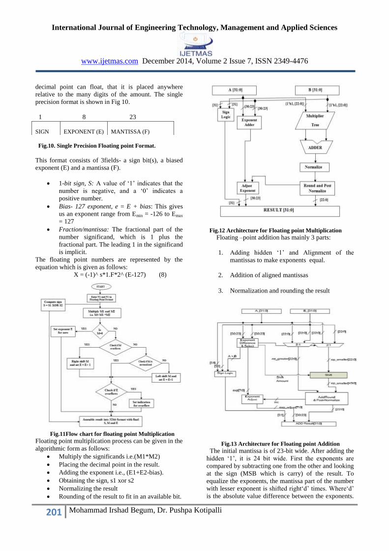
decimal point can float, that it is placed anywhere

relative to the many digits of the amount. The single

precision format is shown in Fig 10.

1 8 23

Fig.10. Single Precision Floating point Format.

This format consists of 3fields- a sign bit(s), a biased

exponent (E) and a mantissa (F).

1-bit sign, S: A value of ‘1’ indicates that the

number is negative, and a ‘0’ indicates a

positive number.

Bias- 127 exponent, e = E + bias: This gives

us an exponent range from Emin = -126 to Emax

= 127

Fraction/mantissa: The fractional part of the

number significand, which is 1 plus the

fractional part. The leading 1 in the significand

is implicit.

The floating point numbers are represented by the

equation which is given as follows:

X = (-1)^ s*1.F*2^ (E-127) (8)

Fig.11Flow chart for floating point Multiplication Floating point multiplication process can be given in the

algorithmic form as follows:

Multiply the significands i.e.(M1*M2)

Placing the decimal point in the result.

Adding the exponent i.e., (E1+E2-bias).

Obtaining the sign, s1 xor s2

Normalizing the result

Rounding of the result to fit in an available bit.

Fig.12 Architecture for Floating point Multiplication

Floating –point addition has mainly 3 parts:

1. Adding hidden ‘1’ and Alignment of the

mantissas to make exponents equal.

2. Addition of aligned mantissas

3. Normalization and rounding the result

Fig.13 Architecture for Floating point Addition

The initial mantissa is of 23-bit wide. After adding the

hidden ‘1’, it is 24 bit wide. First the exponents are

compared by subtracting one from the other and looking

at the sign (MSB which is carry) of the result. To

equalize the exponents, the mantissa part of the number

with lesser exponent is shifted right‘d’ times. Where‘d’

is the absolute value difference between the exponents.

SIGN

EXPONENT (E)

MANTISSA (F)





The sign of the larger number is anchored. In

Normalization, the leading zeroes are detected and

shifted so that a leading one comes. Exponent also

changes accordingly forming the exponent for the final packed floating point result

. The Floating point adder or subtractor is used to add

the partial products generated after each multiplication

operation. Hence both multiplication and addition

operations are performed on the real and imaginary

parts of the complex numbers.

Fig 14. Architecture for SM-MIMO System.

The sequence of N- input binary bits are divided into

group of 3bits each. The left group indicates the active

antenna index and the right group indicates the

modulated symbol.This information is transmitted over

the MIMO channel in the noise free environment. The

Receiver is assumed to have full Knowledge of the

channel and it is indicated as the channel matrix H (k).

The received vector at the input terminals of the

receiver is y (k). For the purpose of demodulation, the

receiver performs the Complex multiplications and

Complex Addition operations between the channel

matrix H(k) and received vector y (k) as g (k) = Hconj

(k)y(k). Here g(k) is the resultant Symbol vector. The

floating point multiplication and addition is carried out

at the receiver to obtain the transmitted symbol matrix

and the position of the active antenna. Here single

precision floating pont format is carried out.

IV.RESULTS A) MATLAB Simulation Results

For the purpose of simulation, a flat Rayleigh fading

channel is assumed with additive white Gaussian noise

(AWGN). The receiver is assumed to have full channel

knowledge. Random binary data of length 10, 00,000

bits was generated. Let us consider first thirty

information bits of transmission data.

Fig15: Sampling index vs magnitude plot of first 30 bits of

transmitting data.

Fig16: Magnitude and phase plots of QPSK symbols

Fig17: Magnitude and Phase plots of channel effected

Symbols





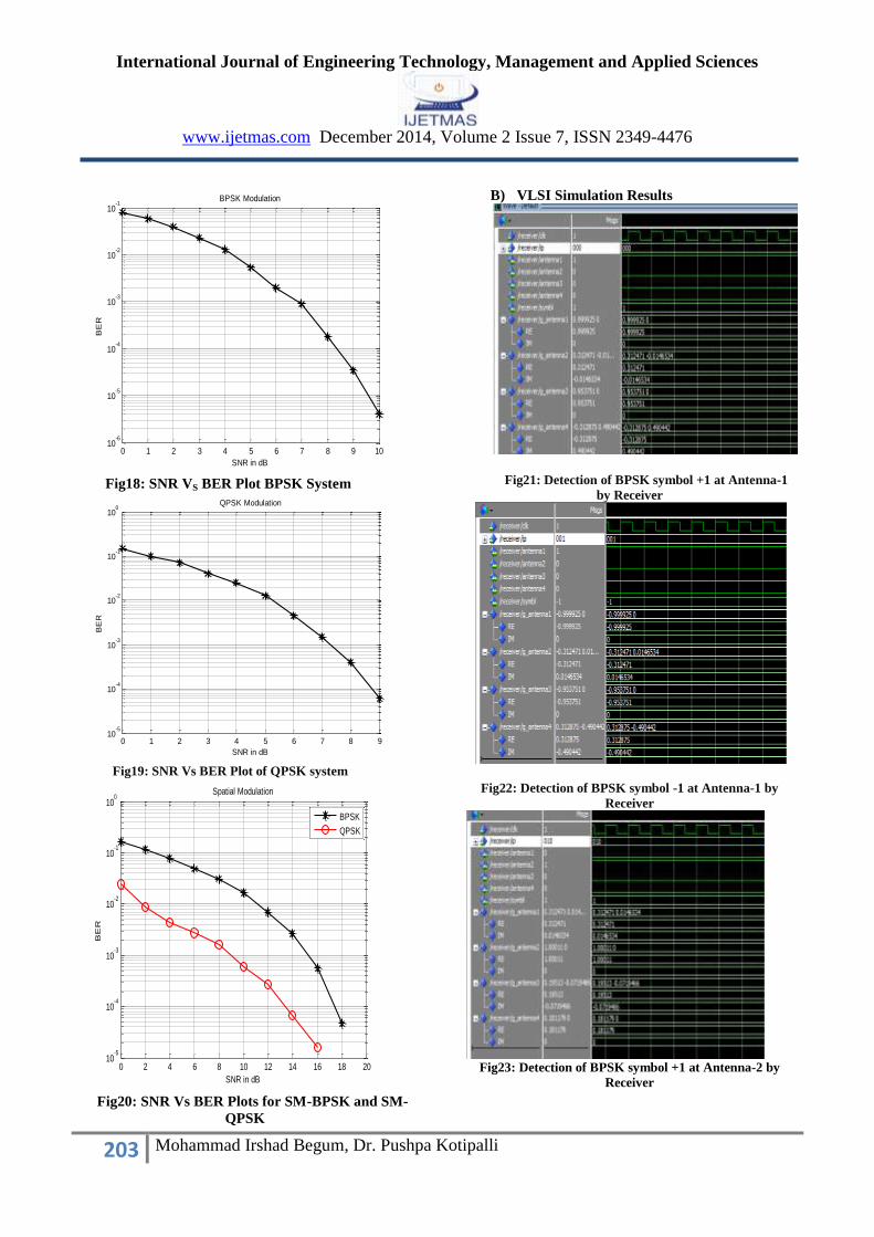
Fig18: SNR VS BER Plot BPSK System

Fig19: SNR Vs BER Plot of QPSK system

Fig20: SNR Vs BER Plots for SM-BPSK and SM-

QPSK

B) VLSI Simulation Results

Fig21: Detection of BPSK symbol +1 at Antenna-1

by Receiver

Fig22: Detection of BPSK symbol -1 at Antenna-1 by

Receiver

Fig23: Detection of BPSK symbol +1 at Antenna-2 by

Receiver

0 1 2 3 4 5 6 7 8 9 1010

-6

10-5

10-4

10-3

10-2

10-1

SNR in dB

BE

R

BPSK Modulation

0 1 2 3 4 5 6 7 8 910

-5

10-4

10-3

10-2

10-1

100

SNR in dB

BE

R

QPSK Modulation

0 2 4 6 8 10 12 14 16 18 2010

-5

10-4

10-3

10-2

10-1

100

SNR in dB

BE

R

Spatial Modulation

BPSK

QPSK





. Fig24: Detection of BPSK symbol -1 at Antenna-2 by

Receiver


Receiver


Receiver


Receiver


Receiver.

Fig29: Detection of QPSK symbol +1+i at Antenna-1 by

Receiver





Fig30: Detection of QPSK symbol -1+i at Antenna-1 by

Receiver

Fig31: Detection of QPSK symbol +1-i at Antenna-1 by

Receiver

Fig32: Detection of QPSK symbol -1-i at Antenna-1 by

Receiver

Fig33: Detection of QPSK symbol 1+i at Antenna-2 by

Receiver.

Fig34: Detection of QPSK symbol -1+i at Antenna-2 by

Receiver

Fig35: Detection of QPSK symbol 1-i at Antenna-2 by

Receiver





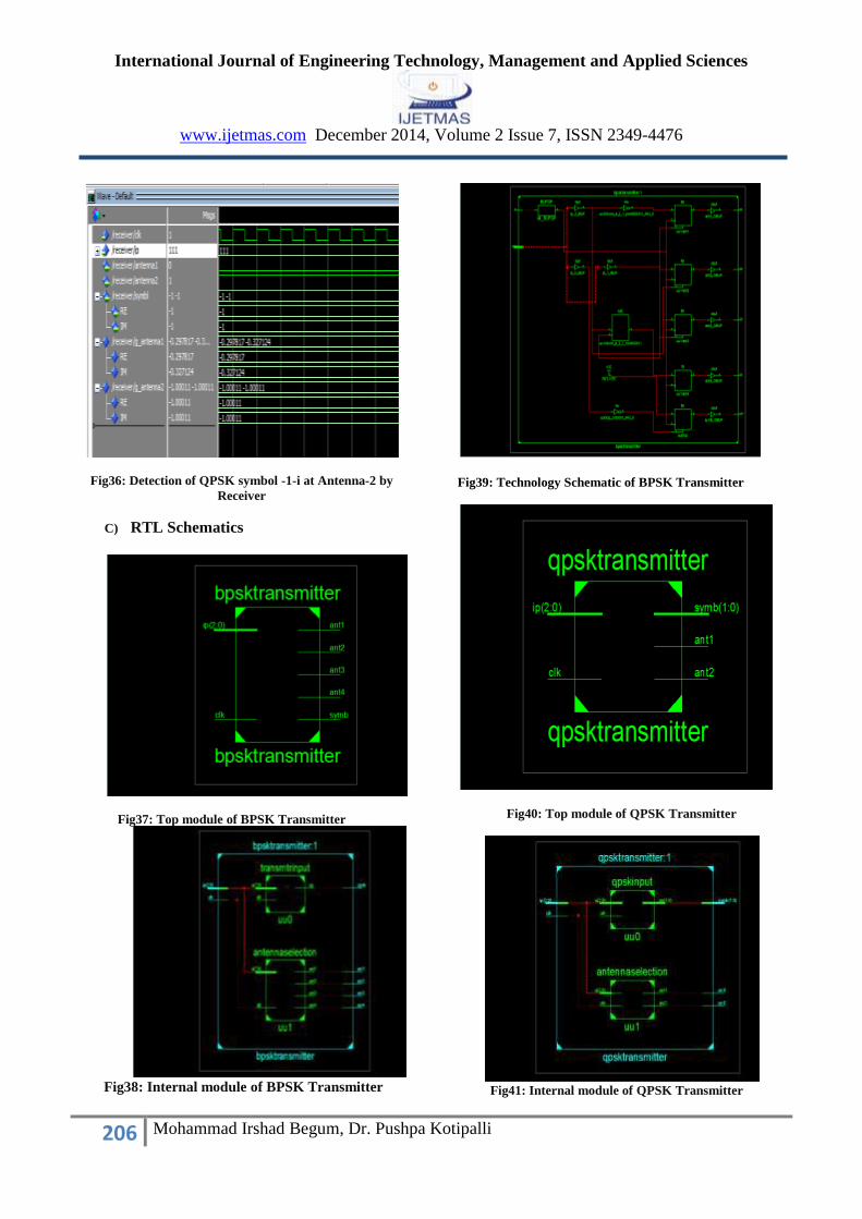
Fig36: Detection of QPSK symbol -1-i at Antenna-2 by

Receiver

C) RTL Schematics

Fig37: Top module of BPSK Transmitter

Fig38: Internal module of BPSK Transmitter

Fig39: Technology Schematic of BPSK Transmitter

Fig40: Top module of QPSK Transmitter

Fig41: Internal module of QPSK Transmitter





Fig42: Technology Schematic of QPSK Transmitter

Fig43: Top module of BPSK Receiver

Fig44: Total Architecture of BPSK Receiver

Fig45: Top module of QPSK Transmitter

Fig46: Total Architecture of QPSK Receiver

Logic

Utilization

QPSK

Receiver

BPSK

Receiver Number of Slices

4353

8826

Number of 4

input LUTs

8630

17492

Number of

bonded IOBs

897

897

Number of

MULT

18X18SIOs

4

4

Number of

GCLKs

1

1

Combinational

Path delay

143.524ns

93.547ns

Fig 47: Comparison Table for BPSK/QPSK Receiver





V.CONCLUSION In this paper, we have implemented the hardware

design of the Spatial Modulation MIMO Receiver with

low complexity using VLSI technology. It employs the

Complex number multiplication and Addition

operations between channel matrix and received signal

matrix. A novel high rate, low complexity MIMO

transmission scheme called Spatial Modulation (SM)

that utilizes the spatial information in an innovative

fashion has been presented. It maps multiple

information bits into a single information symbol and

into the physical location of the single transmitting

antenna. The task of the receiver is to detect the

transmitted symbol and to estimate the respective

transmitting antenna. Spatial modulation avoids ICI at

the receiver input. In addition, only one RF (radio

frequency) chain is required at the transmitter because

at any given time only one antenna transmits. Hence the

energy efficiency is achieved and the cost of the

transmitter is significantly reduced. The Receiver of the

SM-MIMO system has been deigned, which computes

complex number multiplications with less amount of

resources and with low complexity and thereby

achieved high performance.

REFERENCES

[1] Caijun Zhong “Capacity and Performance Analysis

of Advance Multiple Antenna Communication

Systems”, London, March 2010

[2] Raed Y. Mesleh, , Harald Haas, Sinan

Sinanovi´c,Chang Wook Ahn, , and Sangboh

Yun,, “ spatial Modulation”

[3]R.Mesleh, H.Haas, Y.Lee, and S.Yun, “Interchannel

Interference Avoidance in MIMO Transmission by

Exploitng Spatial Information,” Proceedings of the

International Symposium on Personal, Indoor and

Mobile Radio Communications PIMRC

2005,September 11-September 14, 2005

[4] R.Mesleh and H.Haas, “ Spatial Modulation-A

New Low Complexity Spectral Efficiency Enhancing

Technique”, Communication and Networking in China

2006. ChinaCom 06. First International Conference on

25-27, Oct 2006.

[5] M. Di Renzo, Member, IEEE, H.Haas, Member,

IEEE, Ali Ghrayeb, senior Member, IEEE, and Shinya

Sugiura, senior member, IEEE, “Spatial Modulation for

generalized MIMO: Challenges, opportunities and

implementation.

[6] Y.Chau and S-H. Yu, “ Space modulation on

Wireless fading Channels,” Proc.IEEE VTC’2001,

vol.3, pp. 1668-1671, October 2001

[7] J. Jeganathan, A.Ghrayeb and L.Szczecinski,

“Spatial modulation:Optimal detection and performance

analysis,” IEEE Commun.Lett.Vol.12, no.8,pp.545-547,

July 2009

[8] M.D.Renzo and H.Haas, “Performance analysis of Spatial

Modulation,” In Proc. Int. ICST

Conf.CHINACOM,Aug.2010,pp.1-7.

[9] G.Even and P.M. Seidel, “A comparison of three

rounding algorithms for IEEE floating-point

multiplication”, Technical Report EES 1998-8,EES

Dep., Tel-Aviv Univ.,1998

[10] S.Oberman, H. A1-Twaijry, and M.Flynn. The

SNAP project: “Design of floating point arithmetic

units.” In Proceedings of the 13th Symposium on

Computer Arithmetic,volume 13, pages 156–165. IEEE,

1997

[11] dspLog-Signal Processing for communication,

www.dspLog.com

[12] http://www.eng.tau.ac.il/Utils/reportlist/reports

/repfram.htm

[13] www.xilinx.com

[14] Convey Computer corporation, “Convey

computer,” Richardson, TX, 2008-2010 [Online].

Available: http://www.conveycomputer.com


http://www.dsplog.com/

http://www.eng.tau.ac.il/Utils/reportlist/reports%20/repfram.htm

http://www.eng.tau.ac.il/Utils/reportlist/reports%20/repfram.htm

http://www.xilinx.com/

http://www.conveycomputer.com/

vlsi implementation of spatial modulation mimo system...

Documents