vna1 boardnumber = 0, device number =8

1

VNA1

BoardNumber = 0, Device Number =8 HOW TO CALIBRATE AND SAVE DATA

DEVICE HP8753E (30 kHz – 6 GHz)

FRONT PANEL --- CALIBRATION kit 85032B type N

2

THE BUTTONS TO BE PRESSED ARE IN BOLD

Before starting the calibration, you have to set: FREQUENCY BAND: STIMULUS –> START Fmin – STOP Fmax

NUMBER OF POINTS: STIMULUS ->MENU -> NUMBER OF POINTS -> 1601 x1

FILTER IF AVERAGE: RESPONSE -> AVG -> IF BAND -> 3 kHz

To start calibrating: RESPONSE -> CAL

Check that the selected calibration kit is the right one:

CAL-KIT -> SELECT CAL-KIT-> 85032B (N 50 Ω)

CAL -> CALIBRATE -> MENU

FULL 2-PORT

Connect the kit loads to port 1 and 2 of the VNA and start the measurement.

!! THE SEX INDICATED ON THE DEVICE IS THE ONE OF THE CABLE !!

THE PERFORMED MEASUREMENTS ARE UNDERLINED ON THE SCREEN

FORWARD and REVERSE port are signed on the device

REFLECTION FORWARD (OPEN, SHORT, LOAD)

REFLECTION REVERSE (OPEN, SHORT, LOAD)

TRANSMISSION (insert transition F/F) DO BOTH FWD+REF

ISOLATION OMIT

At the end, press the button: Done 2 Port Cal

Calibration has to be saved in one of the 31 available registers.

INSTRUMENT/STATE -> SAVE/RECALL (save type, points, data)

3

CALIBRATION CHECK

To check that the calibration you have done is correct, you can measure the |S11| and |S21| (in dB) of the last element inserted in calibration (transition F/F).

RESPONSE -> MEAS; RESPONSE -> SCALE/REF

Typically, you must find: |S11| < -50 dB and |S21| @ 0 dB in the whole band. Plot S21, phase included. (REPORT).

You can expand the scale using the function SCALE -> AUTOSCALE

Then you can visualize the scattering parameter S11 on Smith Chart.

RESPONSE -> MEAS ->S11; RESPONSE -> FORMAT ->SMITH CHART

The transition F/F will give place to a point in the origin. (REPORT).

As a further verification, you should measure S11 on Smith Chart, leaving port 1 open. How does the open port act? (REPORT).

SAVE DATA

Copy the MATLAB Routines (MatlabRoutines_2019) in a “TempData” folder.

Select the file: DataAcquisition9.m

Open the file and delete the comment (%) to the VA device number you used (VNA1 BoardNumber = 0, DeviceNumber = 8), and to the correspondent dataStruct command.

Press the green button RUN. The acquired data end up in MATLAB Workspace.

Data are stored in the variable called dataStruct.

To save measurements in the current folder (presumably TempData) with the name `NewName` you have to type: save(‘NewName’,’dataStruct’).

To re-load data in MATLAB Workspace, you have to type: load (‘NewName’)

The dataStruct can be saved in a file .mat also from the Workspace variables list, right-clicking on the dataStruct variable.

4

VNA2


STRUMENTO HP8753C (300 kHz – 3 GHz) (3 MHz – 6 GHz)

CALIBRATION kit 85032F type N

5


Before starting the calibration, you have to set: FREQUENCY BAND: STIMULUS –> START Fmin – STOP Fmax

NUMBER OF POINTS: STIMULUS ->MENU -> NUMBER OF POINTS -> 801 x1

FILTER IF AVERAGE: RESPONSE -> AVG -> IF BW -> 3 kHz

To start calibrating: RESPONSE -> CAL

Check that the selected calibration kit is the right one

CAL-KIT (N 50 Ω) -> N 50 Ω

CAL -> CALIBRATE -> MENU

FULL 2-PORT

Connect the kit loads to port 1 and 2 of the VNA and start the measurement.

!! THE SEX INDICATED ON THE DEVICE IS THE ONE OF THE CABLE !!

THE PERFORMED MEASUREMENTS ARE UNDERLINED ON THE SCREEN

FORWARD and REVERSE port are indicated on the device

REFLECTION FORWARD (OPEN, SHORT, LOAD)

REFLECTION REVERSE (OPEN, SHORT, LOAD)

TRANSMISSION (insert transition F/F) (4 measurements)

ISOLATION OMIT

At the end, press the button: Done 2 Port Cal

Calibration has to be saved in one of the 5 available registers.

INSTRUMENT/STATE -> SAVE/RECALL (save type, points, data)

6

CALIBRATION CHECK


RESPONSE -> MEAS->S11 Refl->FWD; RESPONSE->MEAS->S21 Trans -> FWD







SAVE DATA

Copy the MATLAB Routines (MatlabRoutines_2019) in a “TempData” folder. Select the file: DataAcquisition9.m

Open the file and delete the comment (%) to the VA device number you used. (VNA2 BoardNumber = 0, DeviceNumber = 10), and to the correspondent dataStruct = command.






7

PNA


N5230A (10 MHz – 20 GHz)

MANUAL CALIBRATION kit: 85052D type 3.5 mm

ELECTRONIC: E-CAL N4691-60006 type 3.5 mm

8

Before starting the calibration, you have to set:

FREQUENCY BAND: Channel ->Start/Stop -> Start Fmin – Stop Fmax

NUMBER OF POINTS: Sweep -> Number of Points -> 1601

FILTER IF Sweep -> IF Bandwidth -> 3 kHz

MANUAL CALIBRATION

Calibration -> Calibration Wizard

UNGUIDED -> Next

2 Port Solt

View/ Select Cal Kit -> 85052D or 85032F

Connect successively OPEN SHORT LOAD to port 1 and 2 and execute the Thru connection with transition F/F.

!! THE SEX INDICATED ON THE DEVICE, IS THE ONE OF THE LOAD !!

Calibration (State and Cal Set Data *.csa) must be saved in a file inside the group folder. The group folder has to be created in

Desktop -> LaboratoryElectronics1

****************************************************************************************

ELECTRONIC CALIBRATION

To start calibrating click on:

Calibration -> Calibration Wizard -> Use Electronic Calibration (Ecal)

Connect port 1 and 2 of the PNA to the electronic calibration kit.

Next -> 2 port Ecal -> Next -> Measure

Calibration must be saved in a file inside the group folder.

9

CALIBRATION CHECK


RESPONSE -> MEAS; RESPONSE -> SCALE/REF







SAVE DATA



Open the file and delete the comment (%) to the VA device number you used. (BoardNumber = 0, DeviceNumber = 16). Enable the PNA dataStruct line.



To save measurements in the current folder `laboratory` with the name ‘NewName’, you have to type: save(‘NewName’,’dataStruct’).



10

FIELDFOX NETWORK ANALYZER

IP Number = 151.100.44.73 HOW TO CALIBRATE AND SAVE DATA

DEVICE N9916A (30 kHz – 14 GHz)

CALIBRATION kit 85032F Type N

11


To perform MECHANICAL calibration, you have to preset:

FREQUENCY BAND: Freq-Dist –> Start Fmin – Stop Fmax

NUMBER OF POINTS: Sweep ->Resolution -> 1601 x1

To start calibrating: CAL -> Mechanical Cal

Change Cal Type -> 1 port or Full 2 port -> select and Finish

Change Dut Connectors - > Type N

Change Gender -> Dut Port 1 – female -> next port 2

Dut Port 2 – female -> next port

Select Cal Kit ->85032F Type N Cal Kit -> Finish

You have to connect the calibration kit loads to port 1 and 2 of the Field Fox and then perform the calibration. Start Calibration -> Measure -> Finish (at the end)

Calibration must be saved in a device state file. To save it in the computer, use the link at WinSCP on the Desktop.

The device is controlled also by FieldFoxRemoteDisplay on the desktop (file -> connect -> select analyzer ->ok). In this way, on the computer monitor will appear a front panel image of the device that can be used remotely.

You can save data directly on the device (only if it is strictly necessary).

To save data in the working directory (TempData) click on FieldFox icon (WinSCP) in the desktop. A double directory opens. Select on the left TempData and on the right /USERDATA/FILE.

NB: You can save two types of data with the command Save/Recall -> Device -> INTERNAL -> FILE 1) File Type - > PNG (to save the screen-shot) 2) File Type -> Data (CSV) (to save data that they may be processed) Give a name to the file -> click DONE

12

CHECK CALIBRATION (Full-2 port case)

To check that the calibration you have done is correct, you can measure the last element inserted in calibration (transition F/F).

In particular, the magnitude in dB of S11 and S21.

MEAS->S11, MEAS->S21

You must find: S11dB < -50 dB and S21dB @ 0 dB in the whole band. Plot S21, phase included. (REPORT).



MEAS ->S11; FORMAT ->SMITH CHART


As a further verification, you should measure S11 on Smith Chart, leaving port 1 open. How the leaved open port acts? (REPORT).

SAVE DATA



Open the file and delete the comment (%) to the IPaddress you have used, and to the correspondent dataStruct

(FFPNA dataStruct=getdataFFPNA(IPaddress);)






13

R&S SPECTRUM ANALYZER (9kHz, 3 GHz)

IP Number = 151.100.44.144

SAVE DATA

Copy the MATLAB Routines (MatlabRoutines_2019) in the “TempData” folder of the desktop; thus select the file: DataAcquisition9.m

Open the file and uncomment (i.e. delete %) the proper IPaddress line; uncomment also the relevant dataStruct:

dataStruct = getdataRSSPA (IPaddress).






14

To save the spectrum shape in a USB memory, you can use the function after inserting the USB memory in the device: TRACE -> NEXT -> ASCII FILE EXPORT -> select file name and directory from keyboard To capture the screen-shot of the device: HCOPY -> PRINT SCREEN. select file name and directory from keyboard To access to Windows XP, click on: <CTRL><ESC> Documents -> My Documents -> Removable Disk (F:). To come back, press the button minimize at the top right in the screen To access to Windows XP, you can press the button that has Windows icon on the keyboard.

Use only the USB key provided in the laboratory.

15

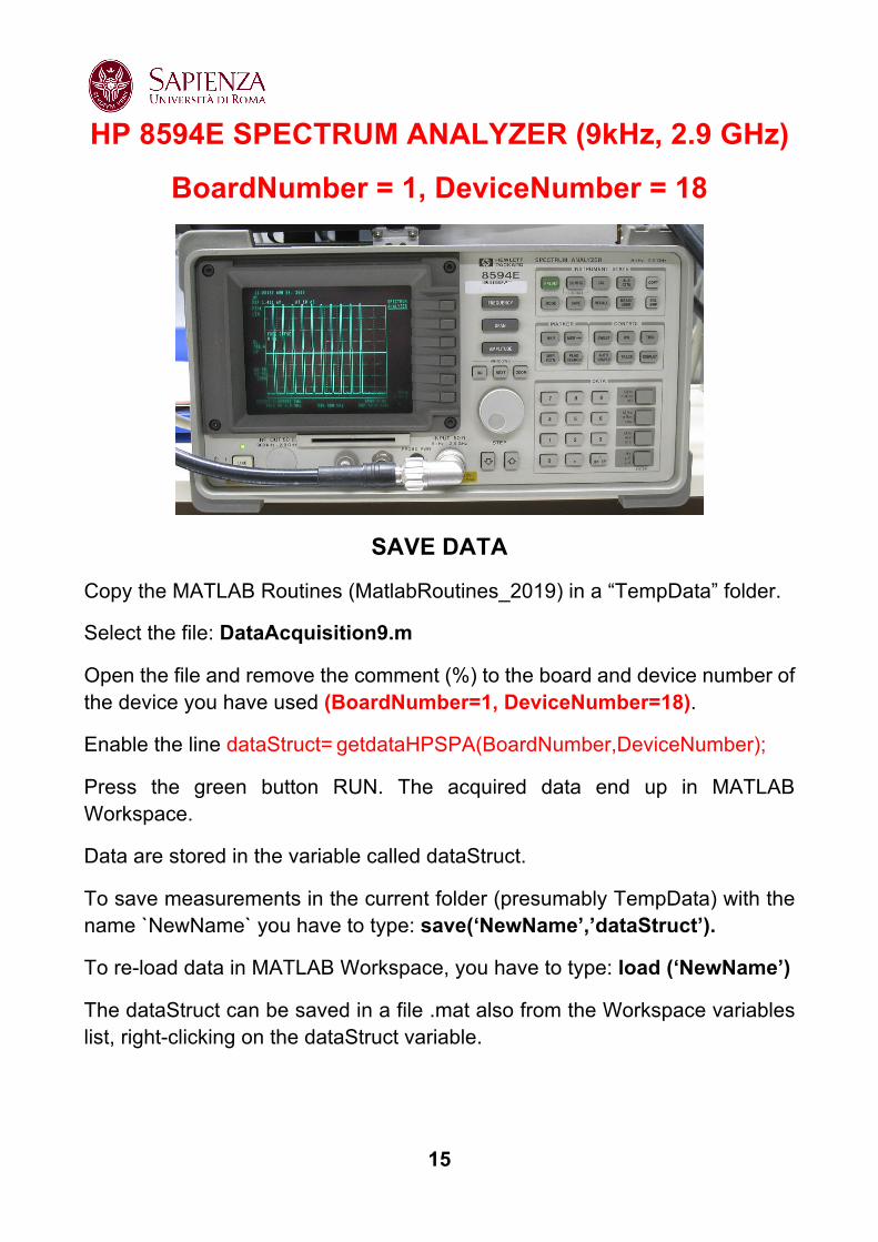
HP 8594E SPECTRUM ANALYZER (9kHz, 2.9 GHz)

BoardNumber = 1, DeviceNumber = 18

SAVE DATA



Open the file and remove the comment (%) to the board and device number of the device you have used (BoardNumber=1, DeviceNumber=18).

Enable the line dataStruct=getdataHPSPA(BoardNumber,DeviceNumber);






16

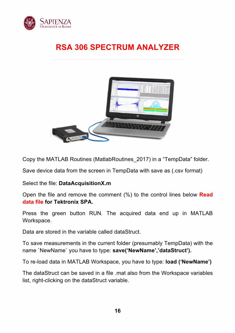
RSA 306 SPECTRUM ANALYZER


Save device data from the screen in TempData with save as (.csv format) Select the file: DataAcquisitionX.m

Open the file and remove the comment (%) to the control lines below Read data file for Tektronix SPA.






17

FIELDFOX NETWORK ANALYZER

IP Number = 151.100.44.28 HOW TO CALIBRATE AND SAVE DATA

STRUMENTO N9918A (30 kHz – 18 GHz)

CALIBRATION kit 85052D type 3.5mm

18


To perform MECHANICAL calibration, you have to preset:

FREQUENCY BAND Freq-Dist –> Start Fmin – Stop Fmax

NUMBER OF POINTS: Sweep ->Resolution -> 1601 x1

To start calibrating: CAL -> Mechanical Cal

Change Cal Type -> 1 port or Full 2 port -> select and Finish

Change Dut Connectors - > Type N

Change Gender -> Dut Port 1 – female -> next port 2

Dut Port 2 – female -> next port

Select Cal Kit ->85032F Type N Cal Kit -> Finish

You have to connect the calibration kit loads to port 1 and 2 of the Field Fox and then perform the calibration. Start Calibration -> Measure -> Finish (at the end)

Calibration must be saved in a device state file. To save it in the computer, use the link at WinSCP on the Desktop.

The device is controlled also by FieldFoxRemoteDisplay on the desktop (file -> connect -> select analyzer ->ok). In this way, on the computer monitor will appear a front panel imagine of the device that can be used remotely.



NB: You can save two types of data with the command Save/Recall -> Device -> INTERNAL -> FILE 1) File Type - > (to save the screen-shot) 2) File Type -> Data (CSV) (to save data that they may be processed) Give a name to the file -> click DONE

19

CHECK CALIBRATION (Full-2 port case)

To check that the calibration you have done is correct, you can measure the last element inserted in calibration (transition F/F).

In particular, the magnitude in dB of S11 and S21.

MEAS->S11, MEAS->S21

You must find: S11dB < -50 dB and S21dB @ 0 dB in the whole band. Plot S21, phase included. (REPORT).



MEAS ->S11; FORMAT ->SMITH CHART

The transition F/F will give place in a point in the origin. (REPORT).

As a further verification, you should measure S11 on Smith Chart, leaving port 1 open. How the leaved open port acts? (REPORT).

SAVE DATA



Open the file and delete the comment (%) to the IPaddress you have used, and to the correspondent dataStruct

(FFPNA dataStruct=getdataFFPNA(IPaddress);)






20

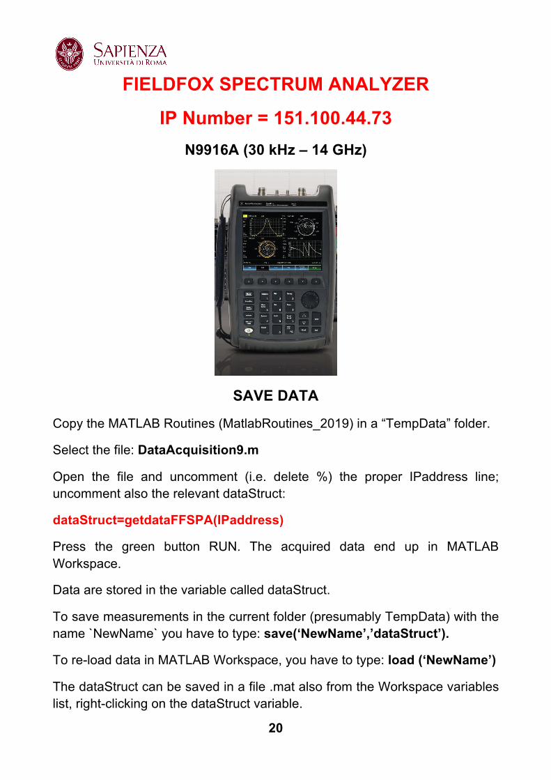
FIELDFOX SPECTRUM ANALYZER

IP Number = 151.100.44.73 N9916A (30 kHz – 14 GHz)

SAVE DATA



Open the file and uncomment (i.e. delete %) the proper IPaddress line; uncomment also the relevant dataStruct:

dataStruct=getdataFFSPA(IPaddress)






21

The device is controlled also by FieldFoxRemoteDisplay on the desktop (file -> connect -> select analyzer ->ok). In this way, on the computer monitor will appear a front panel image of the device that can be used remotely.



NB: You can save two types of data with the command Save/Recall -> Device -> INTERNAL -> FILE 1) File Type - > (to save the screen-shot) 2) File Type -> Data (CSV) (to save data that they may be processed) Give a name to the file -> click DONE

22

ENA NETWORK ANALYZER

BoardNumber = 1, DeviceNumber = 17 DEVICE E5063A (100 kHz – 18 GHz)

SAVE DATA



Open the file and remove the comment (%) to the board and device number of the device you have used (BoardNumber=1, DeviceNumber=17).

Enable the line dataStruct=getdataENA(BoardNumber, DeviceNumber);




