vo um u b r 3 j - 10 - indian association of physics teachers

Vo um u b r 3 J - pt. 10

Editorial

Indian Science and Nobel Prize

The first week of October of each year-when Nobel Prizes are announced by the SwedishAcademy-reminds us to introspect as a ritual on the status ofIndian Science vis-a-vis the world.A gloom descends on the academic horizon, but vanishes soon without leaving any effect on the fu-ture course of Indian science. The question as to why scientists from post- independent India neverearn a place on the Nobel list becomes more perplexing with every passing year especially whenone considers the growing investment in science and Higher Education by the country. The questionoften lurks in our mind why India does not qualify even thoughit could achieve this distinction twodecades before its independence through its epoch making discovery of C.V.Raman in experimentalPhysics with meager facilities. The issue becomes all the more poignant when we recall that pre-independent India produced several luminaries like J.C. Bose, S.N. Bose,M.N. Saha, H.J. Bhabha etal. some of whom the world recognizes as near or equivalent Nobel Laureate. Needless to say thatthis Nobel glory was not confined to science only but extendedto other field as well like literaturewhere Rabindranath Tagore achieved this distinction.

Before 1947 India had about 25 universities devoted mostly to teaching and a couple of researchinstitutes founded and run privately by eminent philanthropic individuals. In the last six decadessince independence India has established about 500 universities, a dozen or so IITs and more thana hundred dedicated research institutes, some of which are fully or partly residential with worldclass infrastructure and facilities. In this scenario, theanswers to the above question often paradedon various forums, are more elusive than real. In popular ethos, Nobel Prize has been heraldedas the ultimate recognition of the brilliance of a creative mind. The dismal performance of Indiain this respect may be considered as a pointer to the opposite, inflicting on us self-doubt and lossof self esteem. However the achievement of Indian mind in thelast 5000 years points out to thecontrary. Rig Veda has been accepted as the oldest book produced by the humanity. India has therare distinction of establishing the first university in theworld at Takshyashila which was flourishingin 500 BC with visiting scholars from other nations. The recent conclusive research by George Ifrahspanning over two decades culminated in the treaties “Universal History of Numbers” translated into14 languages by scholars from Cambridge and Princeton wherehe has finally concluded: “Whileall ancient civilizations struggled for centuries to find a system for writing big numbers India onlysucceeded in discovering decimal place value system and zero, the very corner stone of humanknowledge. Modern science and technology could flourish in the frame work of a number system asrevolutionary and efficient as our positional decimal system which originated in India.” It has beenappropriately termed as “Science of Sciences” by Swami Vivekananda. Such unique contributions,coupled with the fact that four Indians leaving the country after their University education, and whileworking abroad, could win Nobel Prizes, suggests that the answer to the above question may alsopartially lie somewhere else in the depth of our consciousness rather than entirely on the externalmaterial plane.

Out of many factors contributing to the success of human endeavour, the predominant role ofculture is undisputed. Culture is an invisible force, whichdetermines the value system in the society

and shapes human thought, empowering it with dynamism and direction. The momentous questionis “Does the nation have a scientific culture conducive for achievement of excellence in research?” Ithas often been alleged, and also normally accepted, that India is not a meritocracy, the primary causeof which is the underlying trait of cronyism and feudalism innational character inherited from ourpast history. A classic example of the manifestation of thistrait is the case of Hargovind Khuranawho left India in 1950s and sought his fortune in USA eventually being honoured with Nobel Prizein Biophysics. Needless to say it is a fountain head of many evils polluting the academic and publiclife as a whole. It may be argued that other countries were also ruled by kings and emperors and hada feudal past like India. However this force has grown feebleand weak and is almost non-existent inmost of the European countries who have done away with their monarchy centuries ago; and in USA,the most creative country in the world, it never existed since its inception. A more decisive factor forIndia has been its long foreign rule. It is probably the only country, which was invaded and ruled byforeigners for about thousand years. It may be recognized that it is easier to fight empire but difficultto fight with the legacy left by it. When a handful of foreigners rule a huge country like India, theyhave to recruit many natives to the lower level of administration. Those privileged natives servingunder the foreign masters eventually are likely to develop the traits of sycophancy and hypocrisy,which practiced for thousand years get ingrained into the character. These traits manifest on thesurface as cronyism and feudalism, which may be identified asthe invisible evil force plaguing thefree play of national sprit.

The second most impeding factor is Indias religious thought. India made pioneering researchin various branches of science like astronomy, mathematics, chemistry, metallurgy and medicalscience etc, in vedic and post-vedic period extending up to seventh century. However with theadvent of Sankaracharya and his strong revival of Advaita Vedanta philosophy in eighth century,this momentum got redirected to spirituality by the realization that the ultimate truth does not liein external nature but in internal spirit whose study would eventually lead to “mokshya”. Sincethen this has been the mainstay and guiding force in nationalpsyche with obvious adverse effect ongrowth of Indian science.

The third factor is the obsolete Indian Education system based on rote learning and excellencein examination with little stimulation for creativity. This system introduced in mid 1850s designedto produce educated workforce to run colonial rule has almost remained the same defying generallaw of evolution. The fourth factor is the grinding poverty of India posing a barrier for creatingstate-of-the art infrastructure and laboratories at competitive pace with the international science.The upsurge of nationalistic spirit during freedom movement commencing from the last decade ofnineteenth century, could unleash the national psyche fromthe strangle-hold of the evil force for awhile and could overcome the discomfitures posed by the remaining factors giving rise to the goldenera of Indian science and other fields before independence. However soon after independence, thisweakened force finding a level playing field has reappeared with renewed strength. Awareness ofits existence and conscious effort to eradicate it, and together with the appropriate measures to dealwith the other impeding factors may be the national imperative for resurrection of Indian science.

L. Satpathy

85

P R A Y A S c© Indian Association of Physics TeachersStudents’ Journalof Physics

TURNING POINTS

Does Space have more than Three Dimensions?

Sreerup RaychaudhuriTata Institute of Fundamental Research, Mumbai 400 005, India

Communicated by: D.P. Roy

Can this be a serious question? Everyone learns quite early in school that space hasthreedi-mensions, exemplified by the length, breadth and height of a solid object, such as the box in theaccompanying illustration. Later, one learns to representthese dimensions by coordinates, or dis-tances from three fixed planes, and then one is able to denote apoint in space by a triad of realnumbers called coordinates. With a little more mathematical knowledge, we can use any three func-tions of these coordinates (such asr =

√

x2 + y2 + z2, θ = cos−1 z√x2+y2+z2

, ψ = tan−1 yx ) as

coordinates themselves. But the number of coordinates is always taken as three.

Despite this commonsense representation of the space in which we live, from remote antiquitymystic philosophers have speculated on the existence of invisible extra dimensions, where one willbe able to find non-mundane entities such as gods, spirits, etc. Scientists generally do not takesuch ideas seriously – at least from a professional point of view. But nearer home, abstract mathe-maticians freely use spaces of higher dimension, denoting apoint by(x1, x2, . . . , xn) wheren is a(possibly large) integer. Of course, this is believed to be an abstraction not corresponding to a physi-cal reality. In statistical mechanics, physicists borrow the mathematician’s concept to talk of aphase

space, which, for an ideal gas, has the dimension6NA, whereNA ≈ 6.023 × 1023 is the Avogadronumber. Quantum mechanics is formulated in a space ofinfinite dimensions, though this ‘space’ isreally a system of configurations of the physical system. None of these so-called ‘dimensions’ are

86

dimensions ofspace– which we shall henceforth callgeometricdimensions. They just correspondto independent variables describing the system.

Like so much else in modern physics, the scientific question of higher geometricdimensionsoriginated from the transcendent genius of Albert Einstein. In his seminal 1905 paper on the the-ory of Special Relativity, Einstein showed that, for a moving observer, space and time coordinatestransform into one another as

x→ x′= Λxxx+ Λxyy + ΛxzZ + Λxtt

y → y′= Λyxx+ Λyyy + ΛyzZ + Λytt

z → z′= Λzxx+ Λzyy + ΛzzZ + Λztt

ct→ ct′= Λtxx+ Λtyy + ΛtzZ + Λttct

where the coefficientsΛxx etc. are functions only of the velocityv between the two inertial frames,and c, the speed of light in vacuum. Since Special Relativity tells us that all inertial frames areidentical from a physical point of view, it is clear that there is no absolute criterion for determiningwhether the space and time coordinates measured by an observer are “pure” or “mixed” in the abovefashion. This can be elegantly expressed as every event taking place in a four-dimensional spacetimecontinuum with coordinates(x, y, z, ct), a formulation developed by Einstein’s old mathematicsteacher Hermann Minkowski in 1908. The transformation between moving frames of reference,then, is just like a “rotation” in the four-dimensional spacetime.

In Minkowski’s mathematically pretty spacetime, space andtime do get mixed up, but they stillretain their separate identities, like partners in an unhappy marriage. This is because, as everyoneknows, we cannot go back in time – a principle enshrined in physics as the second law of thermo-dynamics. Time is not, therefore, a geometric coordinate inthe same sense asx, y andz are. Thisis often expressed by describing spacetime as having 1+3 dimensions, rather than 4 dimensions.However, in 1914, a young Finnish relativist, Gunnar Nordstrom, showed how it is possible to haveextra geometric dimensions, which are genuine extensions of space. It is possible, said Nordstrom,to havecompactextra dimensions of very small size – smaller than the smallest object which can beseen by any kind of microscope.

Prayas Vol. 4, No. 3, Jul. - Sept. 2010 87

The idea of compactification is as follows. Imagine a flat sheet of paper, and suppose there isan ant crawling along on top of it. The ant is free to move alongthe length and breadth of thepaper and in closed paths if it so desires. If it is an intelligent ant, it will tell us that the space isof two dimensions. Now roll the paper up into a cylinder. The ant can still crawl along the surfacein the straight direction, and at the cost of clinging on for dear life, it can crawl right around thecircular direction. The latter direction (dimension) is said to be “compact” – this means that the antcan come back to its original position by moving forwardsmonotonicallyalong that direction i.e.without reversing its motion. Of course, the ant will recordthe existence of two dimensions, eventhough these two are of somewhat different kinds. However, if we keep rolling up the paper intotighter and tighter cylinders (this is an ideal paper of zerothickness), i.e. reducing the radius of thecylinder (orradius of compactification), there will come a time when the ant is no longer able tocrawl around the cylinder. It can move only along the straight edge, and it will, therefore, concludethat it is in a space of just one dimension. We say (or rather, the ant says) that the two-dimensionalspace has become compactified to one dimension.

One can still argue that if we replace the ant by a flea, which ismany times smaller, or by abacterium or a virus, the latter will be able to ‘see’ the compact dimension, just as the ant was ableto in the earlier analogy. However, if we keep shrinking the radius to smaller and smaller sizes– smaller than the smallest probe we can use – then the compactdimension will be invisible forall practical purposes, but can still exist! According to quantum mechanics, the smallest objectsare ‘seen’ when they scatter matter waves of wavelengthλ = h/p, wherep is the momentumof the matter particles (typically electrons or protons). For the largest values ofp attainable atparticle accelerators at present, this wavelength is around 10−18m, or a nano-nanometre. For radiiof compactification below this limit, matter wave diffraction effects will render invisible one, two orany number of compact dimensions which space may have. Theseare not restricted to be circular,either – any closed (compact) shape will do, so long as we can assign to it a size.

If we cannot ‘see’ them, of what use are such tiny dimensions?A good deal, it turns out. Thepoint is thatgravity can see them! This is because Einstein (again!) taught us to regard gravity notas a field encompassing a passive substrate of spacetime, butas the fabric of spacetime itself. Nord-strom, and his successors Theodore Kaluza (1919) and later Oskar Klein (1926), were able to usethis idea with partial success to develop a unified field theory which incorporated both gravitation

88 Prayas Vol. 4, No. 3, Jul. - Sept. 2010

and electromagnetism. The more successful1 Kaluza-Klein theory required one extra dimension ofcircular nature – somewhat like the rolled-up side of the cylinder we used above as an illustration.If we consider Einstein’s field equations of gravitation (obtainable from his theory of General Rel-ativity) in thesefive dimensions, i.e. 1+3+1 dimensions, where the first 1 is time,the next 3 arethe usual non-compact space dimensions and the last 1 is the compact space dimension, then, in thelimit when the compact dimension becomes very small, these reduce to (i) the 1+3 dimensional Ein-stein equations, which describe ordinary gravitation, plus (ii) Maxwell’s equations which describethe electromagnetic fields. This is a very beautiful result,often called the “Kaluza-Klein miracle”.All that is needed is the existence of a compact dimension, and the assumption that Einstein’s pos-tulate of General Relativity holds irrespective of the space dimension. In a letter to Kaluza in April1919, Einstein wrote “The idea of achieving [a unified field theory] by means of a five-dimensionalcylinder world never dawned on me. At first glance I like your idea enormously.”

It is hard to believe that a theory as beautiful as the Kaluza-Klein theory can be wrong. Butit is wrong! The problem arises because of the huge discrepancy inobserved strength betweengravitation and electromagnetism. The electromagnetic force between two protons is about1038

times stronger than the gravitational force. If we note that1038 is 100 000 000 000 000 000 000000 000 000 000 000 000 then the point is driven home much more forcefully. In the Kaluza-Klein theory, these strengths, not surprisingly2, are related by the radius of compactificationRc,and the observed ratio can only be achieved by makingRc mind-bogglingly small – as small asRc ∼ 10−35m. Now, if we do make this assumption, it can be shown that all matter waves willhave wavelengths of this order, i.e. using de Broglie’s relation λ = h/p we would predict massesof matter particles to be around1025eV/c2, or about 10 000 000 000 000 000 times the mass of aproton. This so-calledPlanck mass3 is around tens of micrograms – the weight of a pollen grain or adust particle. The masses can also be exactly zero. However,the actual masses of protons, electrons,

1Nordstrom’s theory used Newtonian gravity and hence was not relativistic.2Since that is the only parameter in the theory.3The Planck mass can be understood in many ways. Perhaps the simplest way is to say that the proton

had a mass as great as the Planck mass, then the gravitationalforce between two protons would equal the

electromagnetic force between them.


etc. are neither exactly zero, nor anywhere as large as the Planck mass. It follows, then, that, forall its mathematical elegance, the Kaluza-Klein theory cannot be correct. Barely a month after hisearlier letter, a somewhat crestfallen Einstein was writing to Kaluza again: “I respect greatly thebeauty and boldness of your idea. But you understand that, inview of the existing factual concerns,I cannot take sides as planned originally. . .”

In the period between 1950 and 1975, a series of discoveries and successful predictions graduallyestablished that the electromagnetic interaction, as wellas the two kinds of nuclear forces, can benicely described by a class of models which go under the name of gauge theories. Unlike gravitation,which is intimately connected with the structure of spacetime, these theories have a bunch of fields,defined on a passive spacetime substrate, which mix among themselves in a particular way – thetechnical name for this is aninternal symmetry. In order to ensure that the physical world is notchanged by this kind of mixing, we require to introduce some extra fields, which can then be shownto act as a cement between the original fields, i.e. give rise to forces, such as electromagnetismand the weak and strong nuclear forces. In fact, for electromagnetism, it can be argued the gaugetheory arises quite naturally if we combine the ideas of relativity with the probability interpretationof quantum mechanics. Curiously, Einstein, the pioneer of both relativity and quantum theory, wasnot willing to accept the probabilistic interpretation of quantum mechanics, and was not, therefore,willing to accept the approach that led to the gauge theory ofelectromagnetism. He persisted intrying a purely geometric approach, which ultimately failed. This resulted in cutting him off fromthe mainstream of theoretical physics during the last thirty years of his life. There is a moral in thisstory: even if you are a genius, you do need to listen to the voices around you.

With the advent of gauge theories, Kaluza-Klein-style unification became obsolete, since the newgauge theories were elegant and worked better in practice – in fact, they work so well that a partic-ular combination of gauge theories goes today by the name of the Standard Model. However, thependulum now swung the other way. It became impossible to unify gravity with gauge theories, sothat Einstein’s original dream of having a single unified theory describing all the forces in Naturetook a beating. In a kind of desperation, some scientists4 went a step further and speculated thatwe must give up the traditional description of matter in terms of elementary particles. Instead, saidthese theorists, we must imagine the fundamental objects inthe Universe to be one-dimensionalwriggly little things calledstrings. Different oscillation modes of the strings (like harmonics in aguitar string) would appear as different elementary particles, but underlying the particle descriptionof matter and radiation would be a mass of identical strings.String theories, despite their earlypromise and obvious attraction, have run into all sorts of technical difficulties over the last thirtyyears or so. Many of these problems have been solved by invoking more and more esoteric ideas,so that today string theory on its own forms an almost independent branch of physics! It is still adebatable issue whether string theory has really advanced our understanding of the four fundamentalinteractions. However, the part that interests us here is the fact that it was realized very early that

4Joel Scherk, John Schwartz and Tamiaki Yoneya may be regarded as the pioneers of string theory.


one cannot define a consistent string theory in 1 + 3 dimensions. String theories work either in 1 +25 dimensions, or in 1 + 9 dimensions. Where are these other dimensions? Obviously, they must becompact and tiny. Thus string theory brought about a revivalof the discarded ideas of Nordstrom,Kaluza and Klein, albeit in a different avatar.

What saves a string theory from the mass problem which killedthe Kaluza-Klein theory? Thisis the fact that string theory claims that all the elementaryparticles seen so far correspond to themasslessKaluza-Klein modes of a string theory. The fact that the known particles seem to have ac-tually acquired some finite mass is to be attributed to some other source, which would be eventuallyunderstood when we understand the dynamics of interacting strings better. In the Nordstrom andKaluza-Klein theories, there was no room for any interactions other than gravitation and electro-magnetism, so that these models ultimately failed because of their very simplicity. However, thoughstring theory thus sidesteps the mass problem5, the non-zero masses again lie at the very high Planckmass scale of1025eV/c2, which means that they are unlikely to be ever produced in thelaboratory6.Until such masses can be produced (i.e. never!), we cannot confirm if string theory is a correctpicture of Nature.

Till 1998, none of the speculative ideas of the string theorists were taken with much seriousnessby their more hard-boiled colleagues in the particle physics community. In the world of particlephysics, where particles streamed round and round in accelerator tubes, collided and annihilated,were created and decayed, leaving telltale tracks in some photographic emulsion or solid state ar-ray, everything was still governed purely by the gauge theories developed by the 1970s, or by theirsuccessors, which are all grounded solidly in the 1+3 dimensions of Minkowskian spacetime. Unfor-tunately, despite the well-known successes that have won gauge theorists a clutch of Nobel Prizes,all is not order and understanding in gauge theories. The problem arises because gauge theories havetheir own kind of mass problem. In a pure gauge theory, such ashas been constructed and called theStandard Model, all particles are massless – which, of course, is not the case in reality. To get aroundthis, ingenious minds like Yoichiro Nambu, Peter Higgs, Steve Weinberg and the late Abdus Salam,had introducednon-gauge interactions, which go by the technical names of “scalar self-interactions”and “Yukawa interactions”. Moreover, they were forced to include a hitherto undiscovered new par-ticle – the Higgs boson – to mediate this mass generation mechanism. As this article is being written,we are still looking for this Higgs boson. But even assuming it will be found soon, Gerardus tHooft,the Nobel Prize-winning Dutch theorist had pointed out in 1972 that the mass of the Higgs bosonis not stable under corrections due to the quantum nature of the theory, and that its only naturalvalue could be – hold your breath –1023eV/c2, a value which we have encountered before as thePlanck mass! Such a super-high mass for the Higgs boson wouldnot only drag all the other particle

5or sweeps it under the carpet, if you like.6The highest laboratory energy design till now is that of the LHC at CERN, Geneva, which collides protons at

the energy of around1012eV/c2. This is stilltwelve orders of magnitudetoo small than the required to produce

massive excitations in a traditional string theory.


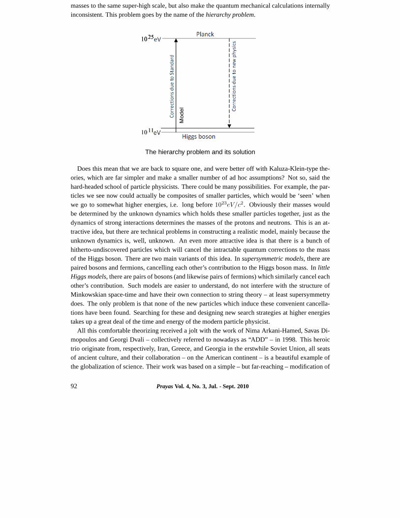
masses to the same super-high scale, but also make the quantum mechanical calculations internallyinconsistent. This problem goes by the name of thehierarchy problem.

The hierarchy problem and its solution

Does this mean that we are back to square one, and were better off with Kaluza-Klein-type the-ories, which are far simpler and make a smaller number of ad hoc assumptions? Not so, said thehard-headed school of particle physicists. There could be many possibilities. For example, the par-ticles we see now could actually be composites of smaller particles, which would be ‘seen’ whenwe go to somewhat higher energies, i.e. long before1023eV/c2. Obviously their masses wouldbe determined by the unknown dynamics which holds these smaller particles together, just as thedynamics of strong interactions determines the masses of the protons and neutrons. This is an at-tractive idea, but there are technical problems in constructing a realistic model, mainly because theunknown dynamics is, well, unknown. An even more attractiveidea is that there is a bunch ofhitherto-undiscovered particles which will cancel the intractable quantum corrections to the massof the Higgs boson. There are two main variants of this idea. In supersymmetric models, there arepaired bosons and fermions, cancelling each other’s contribution to the Higgs boson mass. InlittleHiggs models, there are pairs of bosons (and likewise pairs of fermions) which similarly cancel eachother’s contribution. Such models are easier to understand, do not interfere with the structure ofMinkowskian space-time and have their own connection to string theory – at least supersymmetrydoes. The only problem is that none of the new particles whichinduce these convenient cancella-tions have been found. Searching for these and designing newsearch strategies at higher energiestakes up a great deal of the time and energy of the modern particle physicist.

All this comfortable theorizing received a jolt with the work of Nima Arkani-Hamed, Savas Di-mopoulos and Georgi Dvali – collectively referred to nowadays as “ADD” – in 1998. This heroictrio originate from, respectively, Iran, Greece, and Georgia in the erstwhile Soviet Union, all seatsof ancient culture, and their collaboration – on the American continent – is a beautiful example ofthe globalization of science. Their work was based on a simple – but far-reaching – modification of


the original idea of Kaluza and Klein. Recall that the Kaluza-Klein model had been a model whichsought to unify gravity with electromagnetism through the agency of an extra dimension. The enor-mous masses of the Kaluza-Klein particles had actually arisen because electromagnetism is knownto be enormously stronger than gravitation. What if the extra force due to the extra dimension is notidentified with electromagnetism, but is allowed to be some much, much weaker force? In that case,the masses of the Kaluza-Klein particles could be much, muchsmaller – as small, in fact, as theobserved masses of elementary particles. But, the reader will argue, this would be throwing awaythe initial motivation of Nordstrom, Kaluza and Klein, which was to obtain gravitation and electro-magnetism from the same theory. Never mind, said ADD7. Today we know that electromagnetismcomes from a gauge theory, i.e. an internal symmetry of the quantum fields, and we do not needto generate it out of gravitation, i.e. from a spacetime symmetry. Hence, extra dimensions are notneeded to understand the Standard Model – after all, we have been doing without them for thirtyyears!

Once freed from the shackles imposed by the requirement to generate a theory of electromag-netism, how large can the compact dimensions be? For this, weagain turn to the experimental testsof the Standard Model, which have been performed to great accuracy at a mass scale of around1011eV/c2, which corresponds to a length scale of around10−18 cm. None of these tests show anyevidence whatsoever of extra dimensions. This can be interpreted to mean that either there are noextra dimensions, or, if they exist, they must be compactified to length scales considerably smallerthan10−18 m. This is tiny, but already vastly greater than Kaluza’s value of10−35 m. However,there is a third alternative, which we owe to the ingenuity ofADD. Suppose we have one or moreextra dimensions which are much bigger than10−18 m, but all the particles of the Standard Model(which build up the observable Universe, including our own bodies and instruments) are somehowconfinedwithin the four canonical dimensions of Minkowski and Einstein? Since all our empiricalknowledge comes from these instruments, no ordinary laboratory experiment can show up these ex-tra dimensions. Does this mean that these extra dimensions could be as large as we please, since wedo not see them anyway? Not so, said ADD, because gravity can always see the extra dimensions,just as was argued in the case of primitive Kaluza-Klein theory. The limits on the size of any extra

7Not pronounced ‘add’ but as ‘ay-dee-dee’.


dimensions should come, in ADD’s model of the world, from experiments probing the nature ofgravity, or rather the gravitational force.

Are there such experiments, whose results we can borrow? It turns out that such experimentshave been done ever since the days of Henry Cavendish in the eighteenth century. For if gravitycan propagate in4 + n dimensions, and the extran dimensions are compact with a radiusc, thenNewton’s famous inverse square law of forceV ∝ 1

r would be modified to

V ∝1

r

(

1 +e−r/Rc

r

)

i.e. we would have corresponding changes in the gravitational force between two massive objects.These changes clearly become smaller and smaller asRc → 0. Currently the most accurate mea-surements of this kind come from the Eot-Wash experiment atthe University of Washington, wherea very sensitive torsion balance experiment has been devised by Eric Adelberger and his team ofcollaborators. Their current results show no sign of any deviation from the exact inverse squarelaw, and enable them to determine that if there are extra spatial dimensions, they will have radii ofcompactificationRc < 4.4 × 10−5m. This is much, much larger than the figure of10−18 m. Thelarge value is more indicative of the difficulty of gravitational experiments, than of any fundamentalprinciple. The fact remains, however, that there is no obstacle to having extra dimensions as large as10−5 m, so long as the Standard Model particles remain confined to four dimensions.

Eot-Wash torsion balance

Assuming, then, that we can have an unspecified number of extra compact dimensions as largeas10−5m, how does it matter? How does it affect our four dimensionalworld, where the StandardModel particles and interactions are confined? Profoundly,as it turns out. The fact is that thegravitational lines of force due to a massive source are now uniformly distributed throughout aspace of3 + N dimensions, and only a very few of these intersect the wafer-thin sub-space of 3dimensions, which we call our Universe.

A sketch of the world according to ADD is given above. The horizontal line represents theNextra dimensions, here represented as just one dimension. The full and empty circles at the endsindicate that these two ends are identified, i.e. the extra dimensions are compactified. The thin plane


intersecting this horizontal line orthogonally is the observable three-dimensional Universe. Clearly,its volume forms a very small fraction of the actual volume ofspace and this is what determines thenumber of gravitational lines of force intercepted by our Universe. We conclude then, that this smallvolume is responsible for making the gravitational force extremely weak , i.e. for driving the Planckmass to the extremely high value of1025eV/c2. If we could access the higher dimensions, we wouldsee a much stronger gravitational force, to which corresponds a much smaller Planck mass. In fact,the Planck mass can be shown to reduce drastically in the presence ofN large extra dimensions,following the simple formula

Mp ∼ 102(25−4N)

2+N

(

1m

Rc

)N

2+N

eV/c2

If we setRc ∼ 10−5m, as is permitted by the Eot-Wash experiment, then we have

Mp ∼ 1050−3N

2+N eV/c2

which is around1016 eV/c2 for N = 1, 1011 eV/c2 for N = 2, 108 eV/c2 for N = 3 and evensmaller for more extra dimensions. Clearly, forN = 1, there is still a hierarchy problem, thougha less severe one than the original one. ForN = 2, the Planck scale is now reduced to the preciseexperimental limit. ForN ≥ 3, this value of the Planck scale is inadmissible, and hence wemusthaveRc < 10−5m. For example, forN = 6, having the Planck scale at the experimental limitof 1011eV/c2 would requireRc ∼ 10fm, i.e. the size of a medium-sized nucleus. The importantfact is that by makingRc ∼ 10−5m, or less, we can reduce the fundamental scale (Planck scale)– at which gravity becomes as strong as the electroweak interaction – to about1011 eV/c2. Thisis just beyond the reach of the concluded experiments in particle physics and is about to be testedat the LHC and other machines of comparable energy. Now here is the unique selling point of theADD model. Having such a low Planck mass completely solves the hierarchy problem.Radiativecorrections will drive the Higgs boson mass to some fractionof the higher dimensional Plank mass,rather than the four-dimensional Planck mass discovered byNewton. As this higher dimensionalPlank mass is not so much higher than the experimentally required value of the Higgs boson massthere are no large cancellations, after all.

We see then, that the new paradigm of ADD is based on the following assumptions:


1. Space has3 +N dimensions, of which the3 are the usual dimensions of Euclidean geometryand the otherN are compact dimensions with a radius of less than10−5m (depending onN );

2. The known particles and forces are confined to a subspace ofthe3 usual dimensions, havinga thickness not more than10−18m in the new directions;

3. Only gravity can access the entire space, and by doing so its not-so-small strength in threedimensional space becomes very weak;

4. When we go to very small length scales below10−18m, the Standard Model of particle physicsbreaks down, because at this scale its particles begin to access the full space of3 +N dimen-sions, where strong gravity effects begin to dominate.

Ingenious as they may be, some of the ideas of ADD has been anticipated, in the 1980s, by theJapanese scientist Kei-ichi Akama and by the highly-respected Russian pair of Valery A. Rubakovand Mikhail E. Shaposhnikov. However, these early precursors had different motivations and hadnot thought of their models as solutions for the hierarchy problem. The use of extra dimensions tosolve the hierarchy problem was one of the two things which enabled the ADD paradigm to take thescientific world by storm. The other was its intimate connection with string theory.

I. Antoniadis

The fact that once we can describe electromagnetism by a gauge theory, we do not need to havevery small extra dimensions was known to many workers in the field, but no one really bothered totake it seriously. One researcher who did so was Ignatios Antoniadis, a Greek scientist working inParis, who like his countryman Dimopoulos, is a living proofthat the cradle of Western civilizationhas not lost her ability to produce first-rate scientific minds. Antoniadis, looking for a possibleconnection between string theory and experiments done in the laboratory today, was the first personto explore the phenomenological consequences of having large extra dimensions in the context of astring theory. In the early 1990s, he had written a few papersexploring these ideas, some alone andsome with collaborators, but none of these had really attracted much attention. Now, after the firstADD paper, he was immediately able to team up with its authorsand point out that string theorycould readily provide the mechanism by which the Standard Model particles could be confined toa subspace of three dimensions. This arises because of a peculiarly string-theoretic phenomenon


called aD-brane, which had been discovered just three years before bythe American Joe Polchinskiat the University of California at Santa Barbara. The physical idea for this is simple, though themathematics to describe it is not. Strings, which normally move freely in ten-dimensional spacejust as atoms and molecules can move freely in three-dimensional space, can conglomerate undertheir mutual interactions into lower dimensional objects,just as atoms and molecules can clumpinto sheets and wires. The ends of these congealed string clumps will form a lower dimensionalsubspace, which we call aD-brane.

This is just like the way in which the ends of a sheaf of wheat stalks, as pictured on the right,form a two-dimensional surface, even though the wheat stalks themselves are like one-dimensionalobjects which are free to move in three dimensions. Just as the motion of an insect feeding on the cutends of the stalks would appear as if it were confined to a two-dimensional surface, the behaviourof particles and interactions arising from vibration modesof the strings in the conglomerate wouldappear to be in the lower dimension. If this dimension happens to be three, then the correspondingD3-brane could be what we call our Universe. We can now explain why the particles and forceswhich form the Standard Model of particle physics appear confined to three dimensions – they ariseentirely from the vibration modes of open strings which haveconglomerated into aD3-brane. Onthe other hand, if there is a closed string, like the little loop pictured on the left, then it will be freeto move everywhere in the higher dimensional space. The gravitational field has long been knownto correspond to vibrational modes of closed strings. Hencewe understand why gravity is free topropagate in the higher dimensions.

This combination of a string theoretic mechanism with a neatsolution of the hierarchy problemtook the scientific world by storm. It related the newest ideas in string theory with the century-oldquestion of why gravity is so much weaker than electromagnetism. Moreover, it indicated, as weshall see, a possibility that the strong gravitational effects lurking just outside the confined of ourD3-brane might actually leak a little into laboratory experiments, leading to small effects whichcan be verified at current day experimental facilities such as the Large Hadron Collider (LHC) atGeneva. Let us see how this can arise.

Even if we go back to the simple extra dimensional model of Kaluza and Klein, we encounter the


phenomenon of Kaluza-Klein modes. It is not difficult to understand these. According to Einsteinsspecial theory of relativity, the Newtonian relation between energy and momentum, viz.

E =p2

x + p2y + p2

z

2m

must be replaced by

E2 = p2x + p2

y + p2z +m2

in a system of units where the speed of lightc = 1 (e.g. length is measured in light-seconds). Ifthere is an extra dimension, then this becomes

E2 = p2x + p2

y + p2z + p2

4 +m2

wherep4 is the component of the momentum along the fourth, compact dimension.

Now recall that the wavefunction of a free particle in the extra dimension must describe an integralnumber of wavelengths around the compact dimension, as shown in the figure on the left. In thiscase, we can write the circumference of the extra dimension as

2πRc = nλ

i.e. λ = 2πRc

n wheren is an integer. Using the de Broglie relationλ = 2πh/p4, then, we arrive at

p4 =nh

Rc


i.e. the momentum around the compact direction must be discrete, increasing in steps ofh/Rc. Theenergy-momentum relation now becomes

E2 = p2x + p2

y + p2z +

(

nh

Rc

)2

+m2 = p2x + p2

y + p2z +M2

n

which looks like a set of three-dimensional relations with effective (squared) masses

M2n =

(

nh

Rc

)2

+m2

In most cases of interest,h/Rc ≫ m, so we can neglectm and write, simply,

Mn =nh

Rc.

Thus, a single freely-moving particle in three ordinary andone compact dimension, will appearin three dimensions as a whole set of particles, with masses increasing in steps ofh/Rc. This isoften referred to as a Kaluza-Kleintower of states, and the individual particles are referred to asKaluza-Klein modes. The argument is easily extended intoN extra dimensions to get

Mn ≈h√

n21 + n2

2 + · · · + n2N

Rc

How does this matter for the ADD model? Here most of the particles are confined to threedimensions, and they do not have any wavefunction (probability) extending into the fourth (or more)dimensions. However, there is one particle that does go intothe extra dimension, and that is themassless graviton – the quantum carrying the gravitationalforce in the same way as the masslessphoton carries the electromagnetic force. On theD3-brane, i.e. in the observable Universe, thegraviton will appear, not as a simple massless graviton, butas a whole tower of massive Kaluza-Klein modes of the graviton. IfRc ∼ 10−5 m, this indicates a mind-boggling1030 modes! Thegravitational force between two adjacent particles will then, be not just the force mediated by asingle graviton and leading to Newton’s law with a strength measured by Newton’s constantGN ,but a collective force mediated by literally zillions of Kaluza-Klein modes of the graviton. The netforce will be, not the weak Newtonian force predicted between elementary particles, but a muchstronger force which may become detectable in scattering experiments performed in the laboratory.A schematic picture of this collective interaction in a two-body scattering processA+B → C +D

is drawn below.Such collective interactions could, in principle, be expected to lead to observable effects at high

energy particle accelerators like the Large Electron Positron (LEP) Collider which ran at CERN,Geneva between 1991 – 2001, at the Tevatron, which is runningat Fermilab, USA, since 1994, andat the Large Hadron Collider (LHC) at CERN, which commenced its run last year. Till date, wehave not found any evidence whatsoever for gravitational interactions between elementary particlesof the kind described above. This tells us that if there are, indeed, extra dimensions as hypothe-sized by ADD, their size must be small enough to raise the higher-dimensional Planck scale above


1011eV/c2. However, the LHC, currently operating at a collision energy of7 × 1012eV/c2, couldcertainly probe the hitherto-inaccessible region and tellus if there are, indeed such large extra di-mensions.

What if the LHC does not find any evidence for large extra dimensions, even when it reaches itsfull energy of1.4 × 1013eV/c2? This will not invalidate the theory, but merely push the maximumpossible size of the extra dimensions to a smaller value. However, it will be a disappointing result,in the sense that the model will then become unverifiable, except perhaps in the realm of ultra highenergy cosmic ray studies. Moreover, the ADD construction was discovered, within a year of itsproposal, to have a serious flaw, viz. the large size of the extra dimensions is not stable underquantum corrections. In a manner very reminiscent of the wayin which the Higgs boson mass isdragged to the Planck scale1025eV/c2 by quantum corrections, the size of the extra dimensions isdragged toRc ∼ 10−35m by analogous effects. This would mean that the Planck scale is1023eV/c2

in the3 +N dimensional space as well as on ourD3-brane, and we would be back to where Kaluzaand Klein stood.

Several solutions have been proposed for this problem. One is to invoke supersymmetry to cancelthe troublesome quantum corrections, exactly as was done inthe case of the Higgs boson. The logicfor this is that if theD3-brane is formed in a string theory, then supersymmetry is a natural ingredientin the theory anyway. On the other hand, if there is supersymmetry, we already have a solution to thehierarchy problem, and then the ADD construction does not serve any useful purpose. This is notto say that there cannot be extra dimensions if there is supersymmetry, but normally science doesnot assume things unless we need to. A famous principle enunciated by the scholastic philosopherWilliam of Occam (c. 1288 – c. 1348) states:Entities are not to be multiplied without necessity, andthis is generally known in science as “Occam’s Razor”. Thus,if we have a supersymmetric solutionto the hierarchy problem, the ADD solution would fall foul ofOccam’s Razor8. For this reason,the supersymmetric solution to the problem of stabilizing large extra dimensions has not been verypopular, though no one has challenged it as wrong or impossible.

8However, one must not use Occam’s Razor blindly. It would be like sitting in Mumbai and arguing that

penguins do not exist because they are not needed for the local ecosystem in Mumbai. Nature has surprised us

before and will surely surprise us again.


A much more popular alternative to the ADD construction has been a model with twoD3-branesand one extra dimension, proposed by Lisa Randall and Raman Sundrum in 1999. This collabo-ration, between the all-American Randall and Sundrum, an Australian of Indian origin, is anothertribute to the globalization of science, and especially to the US academic system which is a veritablemelting pot of nationalities. The Randall-Sundrum (RS) model is a bit too technical to be discussedin an article of this nature, but it succeeds where the ADD model fails, in providing a mechanismto control the quantum corrections to the Higgs boson mass without having recourse to large extradimensions. However, the ratio between the gravitational force and the electromagnetic force inthe RS model is now an extremely sensitive function of the radius of compactificationRc. Smalldynamic fluctuations could change this ratio, which is knownto be completely stable. Thus, werequire a mechanism to keep the size of the extra dimension fixed. There is no such mechanismin the original RS model, but an extension devised by Walter D. Goldberger and Mark B. Wise ofCaltech can do the job by introducing an extra scalar field (somewhat like the Higgs boson) whichlives in the full five dimensional space of Randall and Sundrum.

Another suggestion which has found favour in the scientific literature is that of auniversalextradimension. In this model, there are noD3-branes. There is just one extra dimension and all theparticles and forces of the Standard Model can go into the extra dimension. It differs from theKaluza-Klein model in that the extra dimension is not a circle, but is like a circle folded about adiameter. In this theory, every particle has Kaluza-Klein modes, and it is predicted that some ofthese may be discovered at the LHC or other machines, if the radius of compactificationRc is largeenough. There are variations to this model, such as a model with two universal extra dimensions,but the basic ideas are the same.

To conclude, then, extra dimensions of space have progressed from a metaphysician’s dream toan active area of scientific research. Apart from its intrinsic interest, this is a field where variousdisciplines merge. However, only the future will tell if allthis is hard science, or a pretty fiction. Atpresent there is no perfect theory of extra dimensions whichexplains everything and is completelyconsistent internally. But this does not mean that we shouldabandon the search. Saint Augustine,the famous Doctor of the Church, told us long ago that “A thing is not necessarily false because it is

badly expressed, nor true because it is expressed magnificently”. As with all of Western empiricalscience, the proof of extra dimensions will lie in hard experimental facts acquired in the laboratory.We can only look forward to that exciting era.



“Absolute” motion of the earth in the universe

Shubham Agarwal1, Shashank Naphade2 and Ashok K. Singal31 IInd yr., IIT Gandhinagar, Ahmedabad, India. Email: [email protected] IInd yr., IIT Gandhinagar, Ahmedabad, India. Email: [email protected] A&A Division, Physical Research laboratory, Ahmedabad, India. Email: [email protected]

Abstract. In this paper, we determine the velocity of earth with respect to a reference frame in which thedistribution of matter in the universe appears isotropic. We use the distribution of distant radio sources todefine such a reference frame. In particular we look for departuresfrom isotropy in the angular distributionof radio sources in sky as a result of earth’s motion. Our results give adirection of the velocity of earth inagreement with those determined from the Cosmic Microwave Background Radiation (CMBR) measurementsby COBE and WMAP satellites.

Communicated by: A.M. Srivastava

1. INTRODUCTION

Our Earth is not at rest. It goes around the sun and the sun along with the earth and the remainingsolar system bodies, goes around the centre of our Milky Way.The Milky Way in turn has a motionwithin the local group of galaxies, which may itself be moving with respect to the Virgo Super-cluster and so on. If we add all these velocity vectors and thereby get a resultant vector for theearth’s velocity with respect to the largest scale distribution of matter in the universe that may beconsidered to be fixed in the co-moving co-ordinate of the expanding universe, it may be justifiablycalled an “absolute” velocity of the earth. Of course it should be clarified that the word absolutehere does not imply in any sense the presence of the historical “eather” or some absolute space andtime. It is absolute in the sense that there are no further changes in it when we go to still larger scalesin the universe. Then we get velocity of earth with respect toa reference frame which is stationarywith respect to the average distribution of the matter in theuniverse and from which, according tothe cosmological principle, the universe will appear isotropic without any preferred direction.

The earth’s velocity vector in its yearly orbit around the sun is quite accurately known, with themagnitude (∼ 30 km/s) and direction at any time well determined. But the samecannot be said ofthe other velocity vectors. At the same time, while over a year earth’s velocity vector around the sunturns by a complete360◦ to yield an average value∼ 0, the change in all the other vectors is veryminute. For example, in a year the direction of the solar system’s velocity in the orbit around theMilky Way changes by only∼ 6 milli-arcsec [1], implying a change of less than half an arcsec over

102


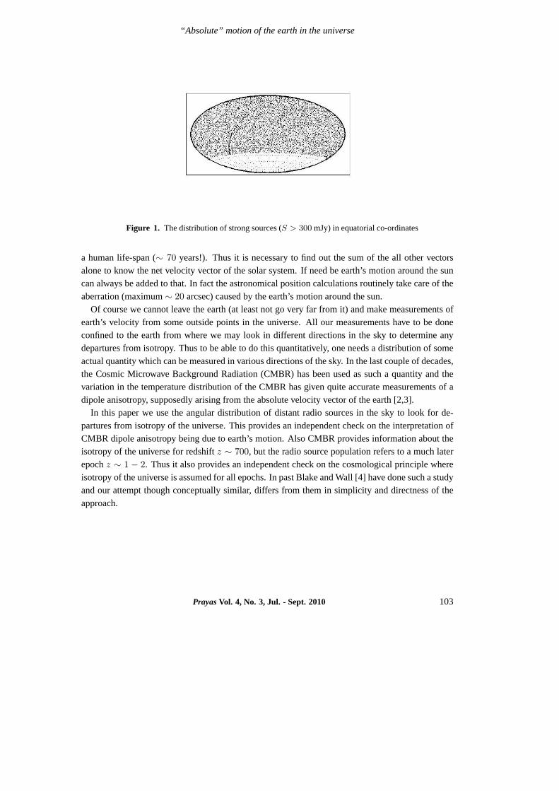
Figure 1. The distribution of strong sources (S > 300 mJy) in equatorial co-ordinates

a human life-span (∼ 70 years!). Thus it is necessary to find out the sum of the all other vectorsalone to know the net velocity vector of the solar system. If need be earth’s motion around the suncan always be added to that. In fact the astronomical position calculations routinely take care of theaberration (maximum∼ 20 arcsec) caused by the earth’s motion around the sun.

Of course we cannot leave the earth (at least not go very far from it) and make measurements ofearth’s velocity from some outside points in the universe. All our measurements have to be doneconfined to the earth from where we may look in different directions in the sky to determine anydepartures from isotropy. Thus to be able to do this quantitatively, one needs a distribution of someactual quantity which can be measured in various directionsof the sky. In the last couple of decades,the Cosmic Microwave Background Radiation (CMBR) has been used as such a quantity and thevariation in the temperature distribution of the CMBR has given quite accurate measurements of adipole anisotropy, supposedly arising from the absolute velocity vector of the earth [2,3].

In this paper we use the angular distribution of distant radio sources in the sky to look for de-partures from isotropy of the universe. This provides an independent check on the interpretation ofCMBR dipole anisotropy being due to earth’s motion. Also CMBR provides information about theisotropy of the universe for redshiftz ∼ 700, but the radio source population refers to a much laterepochz ∼ 1 − 2. Thus it also provides an independent check on the cosmological principle whereisotropy of the universe is assumed for all epochs. In past Blake and Wall [4] have done such a studyand our attempt though conceptually similar, differs from them in simplicity and directness of theapproach.


Shubham Agarwal, Shashank Naphade and Ashok Singal

Figure 2. The distribution of strong sources (S > 300 mJy) in galactic co-ordinates

2. THE SOURCE CATALOGUE

We have used the NVSS catalogue (NRAO VLA Sky Survey [5]) for our investigations. Thissurvey covers whole sky north of declination−40◦, a total of 82% of the celestial sphere,at 1.4 GHz. There are about 1.8 million sources in the catalogue with a flux density limitS > 3 mJy. We have downloaded the NVSS catalogue files by anonymousFTP fromftp://ftp.aoc.nrao.edu/pub/software/aips/TEXT/STARS. The catalog is available in a compact form,giving for each source right ascension, declination and fluxdensity at 1.4 GHz in a tabular form.

Fig. 1 shows a plot of the relatively strong sources (S > 300 mJy) in equatorial co-ordinates.The southern gap is because of theδ > −40◦ limit of the survey. The source distribution looksquite uniform accept for a narrow band of enhanced density presumably due to galactic sources. Toconfirm this, we have plotted in Fig. 2 the source distribution in galactic co-ordinates. The enhanceddensity is now clearly seen to be lying along the galactic plane.

3. ABERRATION

We assume that to an observer on earth without its motion the sky would have looked isotropic, inparticular the radio source distribution would have appeared quite uniform in all directions (ignor-ing a local enhancement due to galactic sources). The motionof the earth will introduce a dipoleanisotropy in this distribution. Due to the aberration of light, the apparent position of a source alongangleθ with respect to direction of motion will actually be shiftedby−β sin θ, whereβ = v/c is thespeed of earth in units of speed of light. Here we have used thenon-relativistic formula for aberrationas CMBR observations indicate thatβ << 1. Forθ = 90◦ the shift is maximum with a magnitude∆θ = β. Thus due to the aberration all sources will have a finite angular shift in their position



towards the direction of motion of the earth. Now if we dividethe sky in two equal hemispheres,one in the forward direction, i.e. centered on the directionof motion of earth, and the second in thebackward direction, then due to aberration some sources from the backward hemisphere, lying in anarrow strip of angular width∆θ = β at the boundary between the hemispheres, will have shiftedto new positions in the forward hemisphere. Thus there will be a larger number of sourcesN1 in theforward hemisphere as compared toN2 in the backward hemisphere. The excess in numbers can becalculated this way. IfN0 is the number density per unit solid angle for the isotropic distribution,thenN1 = 2π N0 + 2π N0 ∆θ andN2 = 2π N0 − 2π N0 ∆θ then the fractional excess in numberof sources will be

∆N

N=

N1 −N2

N1 +N2

=4π N0 ∆θ

4π N0

= ∆θ = β. (1)

Thus we see that the fractional excess in number of sources between the two hemispheres couldprovide a direct measure of the absolute speed of earth. However there are additional complicationsthat need to be considered. The sources in the forward hemisphere will become brighter due toDoppler beaming, while those in the backward hemisphere will become fainter. This will causea telescope of a given sensitivity limit to detect comparatively a larger number of sources in theforward hemisphere. The integral source counts of extragalactic radio source population show thatN(> S), the number density per unit solid angle of sources above a flux densityS, is given by apower lawN(> S) ∝ S−x where indexx may depend upon the flux density level. For a Euclideanuniverse the expected value isx = 1.5. From the NVSS data we have determinedx to be∼ 1.8 forS > 1 Jy and about∼ 1 at weaker levels.

In a non-relativistic case, the frequencyν of photons from a source in directionθ will be shiftedby Doppler factorδ = 1+ β cos θ and the observed flux densityS will be higher than the rest framevalue by a factorδ1+α, whereα is the spectral index defined byS ∝ ν−α. Then as shown in [6],the observed source count due to motion of the earth will showa dipole anisotropy over the sky ofmagnitude[2 + x(1 + α)]β cos θ. Integrating over the two hemispheres, we get

∆N

N= β

[

1 +x(1 + α)

2

]

. (2)

Here we see that apart from the termβ resulting from aberration as described earlier, there areadditional terms arising due to Doppler boosting.

But first we need to find the direction of motion of the earth, otherwise how to know where lies theforward hemisphere and along what great circle to divide thesky in two hemispheres for computingthe excess. A hit and trial method could be tried, but that mayneed too many trials. There is a muchneater way of finding the direction of the earth’s motion.

We consider all sources to lie on the surface of a sphere of unit radius and letr i be the positionvector ofith source with respect to the centre of the sphere. An observer stationary at the centreof the sphere will find the position vectors to be randomly distributed in all directions (due to theassumed isotropy of the universe) and therefore should getΣr i = 0. On the other hand for anobserver on moving earth at that location, due to the dipole anisotropy in number density, the sum


Shubham Agarwal, Shashank Naphade and Ashok Singal

of all position vectors will give a net vector in the direction of earth’s motion, thereby fixing thedirection of the dipole.

The NVSS catalogue has a gap of sources below a declination−40◦. In that case our assumptionof Σr i = 0 for a stationary observer does not hold good. However if we drop all sources fromδ > 40◦ as well, then there are equal and opposite gaps in source distribution on opposite sides of thecelestial sphere andΣr i = 0 is valid for a stationary observer. Thus we confine ourselvesto sourceswithin ±40◦ to determine the direction of motion of the earth. Further wealso excluded all sourcesfrom our sample which lie in the galactic plane (|b| < 10◦). This is because the excess of sourcesin the galactic plane (Fig. 2) is likely to contaminate the determination of the direction of earth’smotion. Of course exclusion of such strips, which affect theforward and backward measurementsidentically, do not affect our results in any systematic manner [6]. We also explored the affect ofany excess of radio sources in the super-galactic plane. We found no discernible difference in thedetermined velocity vector of earth’s motion whether we included or excluded sources in the super-galactic plane.

4. RESULTS

Before proceeding with the actual source sample we created an artificial radio sky with about twomillion sources (similar to the total number of sources in the NVSS catalogue) distributed at randompositions in the sky. We took the flux-density values from theactual NVSS sample, but the skypositions were allotted randomly to each source. Then we randomly assigned a velocity vectorfor earth’s motion and superimposed its calculated aberration effects for each source by shifting itsposition by a small vector∆r i = −β sin θ eθ, whereθ is the angle of the original source positionwith respect to the velocity vector assigned to the earth. The resultant artificial sky was then used tocalculate the velocity vector of the earth which was compared with the value actually assigned. Thisnot only verified our procedure but also allowed us to make an estimate of errors as a large numberof simulations (∼ 50) were run starting with different random sky positions and adifferent velocityvector each time. A realistic estimation of errors was the toughest part of the whole exercise. Thesimulations also allowed us to verify our assertion that rejection of sources at high declinations(|δ| > 40◦) or in galactic plane (|b| < 10◦) did not have any systematic effects on the direction ofthe computed velocity vector. However these gaps in the number distribution raised the computedvalue of∆N/N by ∼ 15%, resulting in the magnitude of the velocity vector being overestimatedby a similar factor.

Our results are presented in Table 1, which is almost self-explanatory. The velocity vector wasestimated for samples containing all sources with flux-density levels> S, starting fromS = 50

mJy and going down toS = 20 mJy levels. Of course the estimate improves as we go to lower flux-density limits, since the number of sources increases asN(> S) ∝ S−x. From Table 1 we inferthatx ≈ 1 at these flux-density levels. But we did not go to still lower flux-density levels as we arenot sure about the completeness of the NVSS sample at those levels. For calculatingβ, we took thetypical spectral index value ofα = 0.8. The calculated RA and Dec for the earth velocity vector are



Table 1. Earth’s velocity vector determined from samples at various flux-densitylevels

S N σN ∆N ∆N/σN ∆N/N RA Dec β

(mJy) (√N ) (N1 −N2) (×10−3) (◦) (◦) (×10−3)

> 50 91597 303 1131 3.7 12.3 171±16 -18±16 5.6±1.5

> 40 115838 340 1218 3.6 10.5 158±14 -19±14 4.8±1.3

> 30 154999 394 1943 4.9 12.5 156±12 -03±12 5.7±1.2

> 25 185477 431 2143 5.0 11.5 158±11 -02±11 5.3±1.1

> 20 229368 479 2836 5.9 12.3 153±10 02±10 5.6±1.0

listed in Table 1 along with the estimated amplitude of the velocity (corrected for the gaps|δ| > 40◦,|b| < 10◦), in units of speed of light. The errors in RA and Dec are estimated from the simulationswhile that inβ are estimated from the expected uncertaintyσN =

√N in ∆N = N1 − N2, the

uncertainty here being that of a binomial distribution, similar to that of the random-walk problem(see, e.g., [7]).

Our estimates of the direction of motion of earth’s velocityvector are in quite agreement withthose determined from the CMBR (RA= 168◦, Dec= −7◦, [2,3]), but our estimate of the magnitudeof the velocity vector somehow appears much higher than the CMBR value (β = 1.23× 10−3). Weare still trying to understand this difference.

ACKNOWLEDGEMENTS

SA and SN express their gratitude to the Astronomy and Astrophysics Division of the PhysicalResearch laboratory Ahmedabad, where work on this summer project was done under the guidanceof AKS.

References

[1] Reid M. J. and Brunthaler A., Astrophy. J., 616, 872 (2004)

[2] Lineweaver C. H., in Proc. of XVI Moriond Astrophysics Meeting, Gif-sur-yvette Publishers, p. 69 (1997)

[3] Hinshaw G. et al., Astrophy. J. Supp. Ser., 180, 225 (2009)

[4] Blake C. and Wall J., Nature 50, 217 (2002)

[5] Condon, J. J. et al., Astr. J. 115, 1693 (1998)

[6] Ellis. G. F. R. and Baldwin, J. E., Mon. Not. R. astr. Soc. 206, 377 (1984)

[7] Reif F., “Fundamentals of Statistical and Thermal Physics”, Chap.1, McGraw-Hill, Tokyo (1965)



Solar Neutrinos and Neutrino Oscillations∗

Himanshu RajIInd yr. Int M.Sc., National Institute of Science Education and Research, Bhubaneswar; NIUS Physics (Batch

6)†

Abstract. The following work was carried out in the NIUS 6.2 and 6.3 winter and summer camps. Webegin with the neutrino production process in the sun and the solar neutrino anomaly as a motivation for theneutrino oscillation. Assuming non-zero neutrino mass, the formal results of the quantum mechanics of neutrinooscillation in vacuum is stated. Then the effect of the ambient matter on neutrino oscillations is considered. TheKamLAND data is then reviewed which pins down the parameters for solar neutrinos. The paper is concludedwith the physics of 3-neutrino oscillations. This formalism along with recent data from solar and KamLANDsuggests a non zero value ofθ13 which hints towards a possible discovery of CP violation in the leptonic sector.

Communicated by: D.P. Roy

1. NEUTRINOS IN THE STANDARD MODEL

The standard model of particle physics in its simplest form enlists the following properties for neu-trinos: i) strict conservation of lepton number, ii) zero mass for neutrinos, and iii) only one helicitystate for the neutrinos. Neutrino comes in three flavors, corresponding to the three generations ofcharged leptonse−, µ− and τ−. These neutrinos namelyνe, νµ andντ are called the flavor orinteraction eigenstate. Thus in the standard model we have 3isospin doublets of left handed leptons

(

νee−

)

L

(

νµµ−

)

L

(

νττ−

)

L

(1)

Neutrino flavor oscillations tend to resolve the long standing solar neutrino anomaly which is ex-plained in the next section. But as we will observe, these flavor oscillations requires that the neu-trinos must have a non-zero mass and that they mix. These ideas lie beyond the confines of thestandard model of electroweak theory. Therefore the resolution to the solar neutrino problem hintsat a new physics beyond the standard model. In the discussionthat follows we assume that neutrinoshave a tiny but non-zero mass without worrying about its origin.

∗A Review†[email protected]

108

Solar Neutrinos and Neutrino Oscillations

2. NEUTRINO PRODUCTION IN THE SUN AND THE SOLAR NEUTRINO ANOMALY

The sun is a main sequence star. It produces an intense flux of electron neutrinos (νe). Energyproduction in the sun takes place through the p-p chain of fusion reactions, which occur at a hightemperature of about1.7× 107 K inside the sun. Protons fuse to form4He nuclei, through variousintermediate nuclear reactions producing high energy photons andνe whose energy is of the orderof MeV. About 99.6% of the total neutrino flux are produced through thepp fusion reaction1. TheStandard Solar Model(SSM), proposed by J. N. Bahcall in the early sixties, predicts the neutrinofluxes from the various intermediate nuclear reactions[2].The figure below depicts the neutrinofluxes along with their energy spectra. Most nuclear reactions produces neutrinos with continuousenergy spectra but neutrinos that are produced through thepep and7Be reactions produce neutrinolines, as they correspond to two body final state. The resulting neutrinos in decreasing order of fluxare (1) the low energy pp neutrinos, (2) the intermediate energy Be neutrinos and (3) the relativelyhigh energy B neutrinos.

Figure 1. The standard solar model (SSM) prediction for the solar neutrino fluxes

shown along with the energy ranges of the solar neutrino experiments.

1An overview of the neutrino production process in the sun can be found inPrayas Vol.4, No.1,Jan.-Mar. 2010

Neutrino Oscillation Phenomenology


Himanshu Raj

2.1 The Solar Neutrino Problem

Since neutrinos have a very small cross-section, their detection is difficult to achieve. However thereare various experimental techniques to detect neutrinos coming from the sun. These are (1) radio-chemical detection, (2) water Cerenkov detection, (3) heavy water detection.

Radiochemical Detection(37Cl and 71Ga): In radiochemical method a target material X, on in-teraction with neutrinos gets converted into a radioactiveisotope of another element Y with half-lifeof several weeks. In a typical run the, the detector is left toabsorb neutrinos for a few week. Thenthe few atoms of the radioactive end product are extracted and counted by using radiochemical tech-niques. By knowing the production cross-section, we can usethe number of produced radioactivenuclei to compute the average neutrino flux. Nuclei that havebeen used for such experiments are37Cl and 71Ga. The earliest solar neutrino detection experiment, led by Raymond Davis, usedthe radiochemical method. The interaction with the solar neutrinos initiates the inverse beta decaycharged current reaction:

νe +37 Cl → e− +37 Ar. (2)

The Q-value for this reaction is 0.814 MeV[3]. According to the prediction of SSM, the dominantcontribution in the chlorine experiment comes from8B neutrinos(75%). But as we can see fromfigure 2 above, the energy of7Be neutrinos just scrapes the threshold energy of the experiment.Therefore a further contribution of 15% comes from the7Be neutrinos.

71Ga is another element used for solar neutrino detection. In theearly 1990s two experimentsstarted producing results using Gallium as an active element in the detector. The reaction is:

νe +71 Ga → e− +71 Ge. (3)

The threshold value of this reaction is 0.233 MeV[3].The product 37Ar and71Ge are radioactivehaving half lives of 34.8 days and 11.43 days respectively. These radioactive end products are peri-odically extracted and measured by Geiger-Muller counters, from which the incident neutrino fluxis estimated. The value of this observed flux R relative to theSSM prediction gives theνe survivalprobabilityPee. The main advantage of the radiochemical method is the low threshold energy of theneutrinos detected. As seen from table 1 below, Gallium detectors have a threshold energy of 0.233MeV, which enables the detection of the pp neutrinos(55 %). Contribution from other neutrinos areBe(25%) and B(10%). Because of this, the capture rate is quite high in Gallium detectors. Althoughradiochemical detection method provided the initial data for the solar neutrino fluxes it cannot deter-mine the energy of the neutrino or the direction that it came from. It is also impossible to determinethe time when a neutrino was trapped in the detector through these experiments.

Water Cerenkov detection: This technique is used in the Super-Kamiokande(SK). The techniquecan detect neutrinos with much larger energy. The detector material is water. The neutrino comesand hits the atomic electrons in hydrogen and oxygen atoms. Since the neutrinos have energies inthe range of MeVs, the atomic binding energies are negligible (∼ eV )and therefore the scatteringcan be treated as elastic scattering of neutrinos off the free electrons:



νe + e− → νe + e−. (4)

The electron recoils with some kinetic energy from the neutrino. If the kinetic energy of the electronis much greater than its mass then it will move at a speed whichis larger than the speed of light inwater thereby emitting Cerenkov radiation in the process. Detection of this radiation constitutes anindirect detection of the neutrino. This method can be used to detect the direction of the incomingneutrino as the Cerenkov radiation has a strong forward peaked angular distribution. By extrapo-lating the cone in the backward direction, it can be verified whether the neutrino is coming fromthe sun. Such detection can be done in ‘real-time’, i.e., theneutrinos can be detected as soon asthey arrive in the detector. This method can detect evenνµ andντ in a neutral current interaction.However, the efficiency of detection is less as compared to that of νe since the cross-sections aredifferent (σ(νµ,τ + e) ≃ 1/6σ(νe + e)). The interaction rate in terms of survival probability is

R = Pee +σNC

σCC + σNC(1− Pee) ≃ Pee +

1

6(1− Pee). (5)

This expression can be inverted to find the corresponding survival probability.Heavy water detection: The technique is employed at the Sudbury Neutrino Observatory(SNO).The experiment uses 1000 tons of ultra-pure heavy water(D2O) contained in a spherical acrylicvessel, surrounded by an ultra-pureH2O shield. Just like the water detectors there are electronsin the atoms whose elastic scattering can be used to detect neutrinos through Cerenkov radiation.However the presence of deuteron opens up more efficient channels of neutrino detection. Deuteron,which is a bound state of a proton and a neutron, has a binding energy of 2.2 MeV, which is in therange of the energy of solar neutrinos. The incoming neutrino can undergo a charged current(CC)reaction with the deuteron as

νe + d → e− + p+ p, (6)

where the information about the neutrino energy and direction can be found by the resulting electrondetected via. its Cerenkov radiation. The Q-value for this reaction is -1.4 MeV and the electronenergy is strongly correlated with the neutrino energy. Thus the CC reaction provides an accuratemeasure of the shape of the8B solar neutrino spectrum. The contributions from the CC reactionsandνee elastic scattering can be distinguished by using differentcos θ⊙ distributions whereθ⊙ isthe angle of the electron momentum with respect to the direction from the sun to the earth. Whileνee have a strong forward peak, the CC events have an approximateangular peak distribution of1-1/3cos θ⊙[3]. A second reaction also takes place in which an incoming neutrino literally breaksup the deuteron into its components. This channel is a neutral current(NC) exchange reaction whosethreshold is the binding energy of the deuteron(2.2 MeV)

νx + d → νx + n+ p (7)

and is open to all active neutrinos. Detection of the resulting neutron via neutron capture confirmsthe occurrence of this process. In neutron capture process aphoton is emitted. The electron comingfrom the Compton scattering of this photon is detected through its Cerenkov radiation. Table 1


Himanshu Raj

below summarizes the energy threshold of the above four experiments along with the compositionsof the corresponding solar neutrino spectra. It also shows the corresponding survival probabilityPee measured by the rates of the charged current reaction relative to the SSM prediction. This

Table 1. Theνe survival probabilityPee measured by the CC event rate R of various

solar neutrino experiments relative to the SSM prediction. For SK thePee obtained

after the NC correction is shown in parenthesis.

Experiment 71Ga 37Cl SK SNO-I

R 0.55±0.03 0.33±0.03 0.465±0.015 0.35±0.03

(0.36±0.015)

Eth (MeV) 0.233 0.814 5 5

Neutrino Composition pp (55%) B(75%) B(100%) B(100%)

Be(25%), B(10%) Be(15%)

table shows that the measured solar neutrino flux is less thanthe SSM prediction. This is the SolarNeutrino Problem. The decrease can be attributed to: i) faulty astrophysics of the sun, or ii) somenew physics fundamental to neutrinos. Oscillations among neutrino flavors and solar matter effecton neutrino oscillations are able to explain all the observed solar neutrino interaction rates.

3. NEUTRINO OSCILLATIONS: BASIC RESULTS

Vacuum oscillationsThe probability for an electron neutrino to oscillate into other flavour is given by2

Peµ(l) = sin2(2θ) sin2(1.27∆m2soll/E), (8)

whereθ is the mixing parameter,∆m2sol is difference between the square of mass eigen values,l

is the distance travelled (in meters) andE is the energy (in MeV). Consequently the oscillationwavelength is

λ = (π/1.27)(E/∆m2) ≃ 2.47E/∆m2. (9)

Therefore for large mixing angle (sin2 2θ ∼ 1)the following pattern of neutrino oscillation proba-

Table 2. Conversion probabilities for different values ofl.

l ≪ λ ∼ λ/2 ≫ λ

Peµ 0 sin2 2θ ∼ 1 (1/2)sin2 2θ ∼ 1/2

2A detailed walkthrough of the quantum mechanics of two neutrino oscillation can be found in Prayas Vol.4,

No.1,Jan.-Mar. 2010Neutrino Oscillation Phenomenology



bility emerges where the factor of 1/2 in the last case comes from averaging over the phase factor.This formalism alone does not account for the observed rates(Table 1). We see that the survival

probability of νe is slightly above 1/2 for the low energy solar neutrino but falls to 1/3 at higherenergy. To understand its magnitude and energy dependence we have to consider the effect of solarmatter on neutrino oscillation.

Matter effectIt was pointed out by Mikheyev, Smirnov and Wolfenstein (MSW)that neutrino oscillation patterncan be significantly affected if the neutrinos travel through a material medium rather than throughvacuum. Since normal matter contains electrons and not any muon or tau, anyνe beam that goesthrough matter undergoes both charged current and neutral current interaction whileνµ andντ onthe other hand interacts with the electrons only through neutral current interaction. Since the neutralcurrent interaction is common to all neutrino flavors, it hasno net effect on neutrino oscillations.On the other hand CC interaction has a profound effect on the neutrino oscillation. Therefore if weinclude the CC interaction as the potential energy term thenthe mass eigenvalues become functionsof the electron density in the sun:

λ1,2 =1

2[A∓

√

(∆m2 cos 2θ −A)2 + (∆m2 sin 2θ)2], (10)

where

A = 2√2GFNeE,

andGF is the Fermi coupling. The electron density at the solar coreis N0 ∼ 6× 1031m−3[2], andit decreases roughly in an exponential manner as we move out of the solar core3. The variation ofthese eigenvalues as functions of the solar electron density is plotted in figure 2. The two eigenvalueshowever never actually cross. There is minimum gap given by:

Γ = ∆m2 sin 2θ (11)

This implies that aνe produced at the solar core will come out asν2 provided the transition proba-bility between the two energy levels remains small. Theνe produced at the solar core is dominatedby theν1 component. However at the critical density region, there isa resonant conversion betweenthe two components. After passing through the critical density region, theνe continues to follow theupper eigen value curveλ2 and the neutrino comes out from the sun asν2 with

Pee = sin2 θ (12)

3In fact except for the inner 10% of the radius the best fit equation for the solar electron density as a function

of the radiusR is given byNe/Na = 245exp(−10.54R/R⊙)[2], whereR⊙ = 6.96× 108m is the radius of

the sun andNa is the Avogadro’s number.


Himanshu Raj

Figure 2. Effective mass(energy) eigenvalues as functions of the solar electron density

at small mixing angle.

provided the transition probability between the two levelsremains small throughout the propagation.The most important region for this transition is the critical density region, where the gap betweenthe two levels is the smallest. This transition probabilityis given by the Landau-Zenner formula. Itrelates the transition rate T to the above gapΓ by the relation

T = e−π2γ (13)

whereγ is given by

γ =λc(dλ1/dl)c

Γ∝ λc(dNe/dl)c

N ce

(14)

andλC represents the oscillation wavelength in matter in the critical density region. If the solarelectron density varies so slowly that the resulting variation in the1st eigenvalue over an oscillationwavelength is small compared to the gap between the two, thenγ ≪ 1 and the transition rate isexponentially suppressed. This is called the adiabatic condition. Thus the two conditions for thesolarνe to emerge asν2 together give,

∆m2 cos(2θ)

2√2GFN0

e

< E <∆m2 sin2(2θ)

2 cos(2θ)(dNe/dlNe)c. (15)

The figure below shows the triangular region in the∆m2 − sin2 2θ plot satisfying the above condi-tion. The horizontal side of the triangle follows from the first inequality, which gives a practically



constant upper limit of∆m2 in terms of the solar core electron density, sincecos2 2θ ≃ 1. The sec-ond inequality (adiabatic condition) gives a lower limit onsin2 2θ, determined by the solar electrondensity gradient. Moreover since this condition implies a lower limit on the product∆m2 sin2 2θ,it corresponds to a diagonal line on the log-log plot. The vertical side of the triangle is simply thephysical boundary corresponding to maximal mixing. This isalso called the MSW triangle. The

Figure 3. The positions of the MSW triangle, the earth regeneration effect and the

vacuum oscillation maximum are shown for E = 1 MeV along with the positions ofthe

SMA, LMA, LOW and VAC solutions.

indicated survival probabilities outside the triangle follows from vacuum oscillation formulae, whilethat inside corresponds to equation 12. ThusPee < 1/2 inside the MSW triangle and> 1/2 outsideit, except for the oscillation maximum at the bottom, where the survival probability goes down tocos2 2θ. Finally, the earth matter effect gives a small but positiveνe regeneration probability, whichmeans the sun shines a little brighter at night in theνe beam.

3.1 The four solutions: SMA, LMA, LOW and VAC

Figure 3 marks four regions in the mass and mixing parameter space, which can explain the mag-nitude and energy dependence of the survival probabilityPee shown in Table 1. They correspondto the so called Large Mixing Angle (LMA), Small Mixing Angle(SMA), Low Mass (LOW) andVacuum Oscillation (VAC) solutions. For the LMA and SMA solutions (∆m2 ∼ 10−5eV 2) the lowenergy Ga experiment (E≪ 1 MeV) falls above the MSW triangle in∆m2/E, while the SK and SNOexperiments (E≫ 1 MeV) fall inside it. Therefore the solar matter effect can explain the observeddecrease of the survival probability with increasing energy. For the LOW solution the low energy


Himanshu Raj

Ga experiment is pushed up to the region indicated by the dashed line, where it gets an additionalcontribution to thePee from the earth’s regeneration effect. Finally the VAC solution explains theenergy dependence of the survival probability via the energy dependence of the oscillation phase inequation 8. Figure 4 shows the predicted survival probabilities for the four solutions as functions ofthe neutrino energy. The LMA and LOW solutions predict mild and monotonic energy dependence,while the SMA and VAC solutions predict very strong and non-monotonic energy dependence. The

Figure 4. The predictedνe survival probabilities for the SMA, LMA, LOW and VAC

solutions.

survival rates in Table 1 show a slight preference for a non-monotonic energy dependence, sincethe intermediate energy Chlorine experiment shows a littlelower survival rate than SK. Thereforethe SMA and the VAC solutions were the early favorites. However, the situation changed with themeasurement of the energy spectrum by SK as shown in the plot below[9]. It shows practicallyno energy dependence in the 5-15 MeV range in clear disagreement with the SMA and the VACpredictions of figure 4. This was supported by the charged current data from SNO. So the SMA andVAC solutions were ruled out in favor of the LMA and LOW. We also see from Figure 4 that theLOW solution cannot account for the entire drop of the survival probability with energy from 0.55to 0.35. But we could blame the low survival rate seen by the Cl, SK and SNO CC reactions partlyon the large uncertainty in the Boron neutrino flux of the SSM (Fig.1). This changed however withthe publication of the neutral current data by SNO. Being flavor independent, the NC reaction isunaffected by neutrino oscillation; and hence it can be usedto measure the boron neutrino flux. Themeasured flux was in agreement with the SSM prediction and significantly more precise than thelatter. Using this flux in a global fit to the solar neutrino data essentially ruled out LOW in favor of



Figure 5. Energy dependence of the SK spectrum

the LMA solution. A further confirmation of the LMA solution came from the reactor anti-neutrinodata of the long baseline KamLAND (KL) experiment. It is a kiloton liquid scintillator experimentdetectingνe from the Japanese nuclear reactor through the charged current interaction

νe + p → e+ + n. (16)

It also measures the incidentνe energy through the visible scintillation energy produced by thepositron and its annihilation with the target electron i.e.

Evis = E +me +mp −mn = M − 0.8MeV. (17)

The KL data, taken together with the global solar neutrino data gives a precise estimate of both themass and the mixing angle parameters:

∆m2sol = ∆m2

12 = 7.7× 10−5eV 2, sin2 θsol = sin2 θ12 = 0.33 (18)

4. THREE-NEUTRNO OSCILLATION

In the quantum mechanics of solar neutrino oscillation, we assume that aνe oscillates into a statewhich is a superposition ofνµ andντ . However, since, mixing takes place among all the three flavorof neutrinos, we now consider 3-neutrino formalism. The mass eigenstates,νi are related to flavoreigenstates,να through a unitary matrix U by the relation,

να =∑

U∗

αiνi (19)


Himanshu Raj

where U is often denoted asUPMNS, after the authors Pontecorvo-Maki-Nakagawa-Sakata. In thegeneral 3-neutrino oscillation case a3× 3 mixing matrix can be parameterized by the three mixinganglesθa, θx, θs and three phasesδ, φ2, φ3. If neutrinos are Dirac fermions, as assumed by thestandard model, one of these phase factors(δ) can be absorbed in the wave function of the neutrinostates. However neutrino and anti-neutrino might be two states of the same particle, namelyMa-jorana particles. In this case two more phases, which are called Majorana phasesφ2 andφ3 arephysically observable. These phases are irrelevant for oscillation and matter effects but they becomeobservables in neutrino-less double beta decay. A frequently used parametrization of the U matrixis the following matrix product

U =

1 0 0

0 ca −sa0 sa ca

cx 0 −sxeiδ

0 1 0

sxe−iδ 0 cx

cs −ss 0

ss cs 0

0 0 1

1 0 0

0 eiφ2/2 0

0 0 ei(δ+φ3/2)

(20)

whereci denotescos θi andsi denotessin θi. The angleθa, here denoted asθ23, governs the oscilla-tions of atmospheric neutrinos, the angleθs (θ12) describes solar neutrino oscillations, and the angleθx (θ13) is an unknown angle that is bounded by reactor neutrino experiments at short distances (L≃ 1 km). Vacuum neutrino oscillations probability are given by[4]

P (να → νβ) =

∣

∣

∣

∣

∣

∑

i

U∗

αie−

im2

iL

2E Uβi

∣

∣

∣

∣

∣

2

(21)

where the mi are the neutrino eigenmasses. The oscillation probabilities depend however only ondifferences of squared neutrino masses. Expanding this expression we get

P (να → νβ) = δαβ − 4∑

i>j

Re(U∗

αiUβiUαjU∗

βj) sin2

(

δm2ij

L

4E

)

+2∑

i>j

Im(U∗

αiUβiUαjU∗

βj) sin

(

δm2ij

L

2E

)

whereδm2ij= m2

i−m2

j. This is the oscillation probability forneutrinos. To obtain the correspond-

ing oscillation probability foranti-neutrinos we observe thatνα → νβ is the CPT-mirror image ofνβ → να. Thus if we demand CPT invariance then we have

να → νβ = νβ → να. (22)

Now from the above equation for neutrino oscillation probability we see that

P (νβ → να;U) ≡ P (να → νβ ;U∗). (23)

Hence assuming CPT invariance holds,



P (να → νβ ;U) = P (να → νβ ;U∗). (24)

That is, the probability for oscillation of an anti-neutrino is the same as that for a neutrino, exceptthat the mixing matrixU be replaced byU∗. Therefore the oscillation probability for anti-neutrinobecomes

P (να → νβ)= δαβ − 4∑

i>j

Re(U∗

αiUβiUαjU∗

βj) sin2

(

δm2ij

L

4E

)

−2∑

i>j

Im(U∗

αiUβiUαjU∗

βj) sin

(

δm2ij

L

2E

)

We see that if U is not real, the probabilities for neutrino oscillation να → νβ and for the corre-sponding anti-neutrino oscillationνα → νβ , will in general differ because of the sign difference inthe third term of oscillation probability formula. Sinceνα → νβ andνα → νβ are CP-mirror-imageprocesses, this difference will be a violation of CP invariance. Therefore neutrino oscillations pro-vides a definative test of the possible discovery of CP violation in the leptonic sector.Dnoting the oscillation arguments for the atmospheric and solar phenomena by

∆a ≡ δm2aL

4E,∆s ≡

δm2sL

4E

respectively whereδm2a = m2

3 − m21, δm2

s = m22 − m2

1, the νe survival probability for threegeneration is obtained to be[5]

P (νe → νe)= 1− sin22θxsin2∆a − (c4xsin

22θs + s2ssin22θx)sin

2∆s

+s2ssin22θx(

1

2sin2∆ssin2∆a + 2sin2∆asin

2∆s)

We can see that this formula reduces to Eq. (8) for∆a = θx = θa = 0. The measurement of thethird unknown leptonic mixing angle is a crucial step towardthe possible discovery of CP violationin the leptonic sector. We get the first hints ofθ13 > 0 from the Solar+KamLAND neutrino data.Oscillation of solar and KamLAND (anti)neutrinos do show a weak dependence onθ13. From theatmospheric neutrino data we know thatδm2

31 ≫ δm221, therefore the three-neutrino oscillation

survival probability relevant for both solar and KamLAND (anti)neutrinos is approximately givenby[6]

P 3gee ≃ cos4 θ13P

2gee + sin4 θ13 (25)

whereP 2gee is the νe survival probability in the case of two-neutrino oscillations. P 2g

ee for highenergy8B neutrinos is∼ fB sin2 θ12 wherefB is the8B neutrino flux. For the KamLANDP 2g

ee

is the usual two-generation vacuum oscillation probability 1 − sin2(2θ12) sin2(δm2

12L/4E). Thusfor solar neutrinos an increase inθ13 would imply an increase inθ12 whereas for KamLAND anincrease inθ13 would imply a decrease inθ12. This opposing trendis observed in their respectivedata. The Fig. 6 below shows this trend[7]. This combinationof solar data and the long baseline


Himanshu Raj

reactor data suggests a weak preference for a non-zero valueof sin2 θ13, which arises as a result of aslight difference between the best-fit values ofsin2 θ12 in the two data sets. The best fit values fromthe solar neutrino data is[8]

sin2 θ12 = 0.33, fB = 0.84. (26)

whereas the KamLAND data yields

sin2 θ12 = 0.39 (27)

As a result of non-zeroθ13, θ12 of the solar data decreases while that of the KamLAND data

Figure 6. Effect of nonzeroθ13 on the regions separately allowed by the latest avail-

able data(2008) from the solar and KamLAND experiments, at 1, 2 and 3σ levels.

decreases to settle at some intermediate value determined by the magnitude of the third mixingangle. The present standing value of this angle is

sin2 θ13 = 0.021± 0.017 (at1σ) (28)

for the Solar+KamLAND data.

Acknowledgment

I am greatly thankful to my mentor prof. D.P. Roy, under whom my NIUS Camp was carried out.My hearty thanks to Prof. M. K. Parida who gave me valuable comments on the report specially onthe section of Three Neutrino Oscillation.

References

[1] D.P. Roy, ‘Eighty Years of Neutrino Physics’, Physics News, Vol.39, No 3, p 51 (2009)[hep-ph/0809.1767].



[2] John N. Bahcall, ‘Neutrino Astrophysics’, Cambridge University Press, (1990).

[3] C. Amsler et al. (Particle Data Group), Phys. Lett. B667, 1(2008) (URL: http://pdg.lbl.gov).

[4] Boris Kayser, ‘Neutrino Physics’ (2004) [hep-ph/0506165v1].

[5] V. Barger, D. Marfatia and K. Whisnant, Progress in the physics ofmassive neutrinos, (2003) [hep-

ph/0308123v2].

[6] A. Bandyopadhyay, S. Choubey, S. Goswami, S. T. Petcov and D.P. Roy, (2008) [hep-ph/0804.4857v1]

[7] G.L. Fogli et al 2010 J. Phys.: Conf. Ser.203 (2010) 012103.

[8] G.L. Fogli, E. Lisi, A. Marrone, A. Palazzo, A.M. Rotunno (2009)[hep-ph/0905.3549v2].

[9] D. P. Roy, Solar neutrino oscillation - an overview,, Proc. PASCOS-X, Boston (2004) 150 [hep-

ph/0409336].



PROBLEMS IN PHYSICS

Readers are invited to submit the solutions of the problems in this section within two months. Correct

solutions, along with the names of the senders, will be published in the alternate issues. Solutions

should be sent to: H.S. Mani, c/o A.M. Srivastava, Institute of Physics, Bhubaneswar, 751005;

e-mail: [email protected]

Communicated by H.S. Mani

Problem set by H.S. Mani

1. Consider a hydrogen atom confined inside a thin uncharged conducting shell of radiusR.AssumingR >> aH , whereaH is the Bohr radius. The proton ( assumed infitely heavy) is atthe centre of the shell.

Find the first nonvanishing correction to

i. The radius of the hyderogen atom assuming Bohr quantization rule.

ii. The energy of the ground state.

2. A square cardboard of lengthL is intially at x = 0 has its corners at(0, 0, 0), (0, 0, L), (0, L, L) and (0, L, 0) and moves with a velocity~u = ui. Rain is com-ing vertically down at constant velocity~w = −wk. If the number of drops per unit volume isN , find the number of drops collected by the cardboard as it travels a distanceD.

Viewing the same from the cardboard’s rest frame (assume relativistic velocities), show thatyou get the same result for the number of drops collected by the card board.

135

Problems in Physics

Solutions to the problems given in Vol.4 No.1

Solutions provided by: H.S. Mani

Problem 1: Consider a pencil (length L = .2m, mass 0.05Kg.) standing vertically on its tip, whichcan be considered as a point.Using the uncertainty principle estimate the time it can stay up withoutfalling. Assume the tip is fixed during the fall.

Solution to Problem 1:Let the pencil make an angleθ0 with the vertical and let its initial angular velocityω0. Then thecenter of mass is at

∆x =Lθ02

;∆p =mLω − 0

2

Unvertainty principle demands

mL2θ0ω0

4≥ h

2

If the pencil makes an angleθ with the vertical the torque about the tip ismgl sin(θ)/2, g being theacceleration due to gravity and so we have

Id2θ

dt2=mL2

3

d2θ

dt2=mgL sin(θ)

2

Assume the angle is smallsin(θ) ≈ θ and we get

d2θ

dt2=

3g

2Lθ

Solving the differential equation and using the initial condition to determine the integration constantswe have

θ =θ0 + ω0τ

2et/τ +

θ0 − ω0τ

2e−t/τ

whereτ =√

2L/3g

≥θ0 +

2hτL2θ0m

2et/τ +

θ0 − ω0τ

2e−t/τ

The minimum of the expression(θ0 + (2hτ)/(L2θ0m)) occurs atθ0 =√

2h(τ/L2m). Thus

θ ≥√

2hτ

L2et/τ


Problems in Physics

Even though we have solved the problem for small]theta we can get the order of magniture of thetime of fall by using it for estimating the time of fall by choosingθ = π/2.

π

2≥ 2

√2hτL2met/τ

or

t ≤ τ

(

ln(π

4+

1

4ln

3gm2l2

8h2

)

substitution the number thet ≤∼ 1.7 sec, which is macroscopic!

Problem 2: Consider a one dimensional motion of a particle along the x-axis under the action ofa potentialV (x) = V0 > 0 for x ≤ 0 andV (x) = 0 for x > 0.If the particle moves to the rightfrom x < 0, with an energy2V0 , standard quantum mechanics gives for the reflection coefficient atx = 0 of the order0(1) (The exact number is( (

√

2−1)

(√

2+1))1/2 and the result is independent of the mass

of the particle.Now consider a car travelling with a speedv towards a cliff (heightH). From the previous

calculation the probability of reflection atx = 0 should be0(1) (Assume the kinetic energy of thecar to be of the same order asmgH wherem is the mass of the car). This is an absurd result. Do acorrect modeling for the cliff and obtain a physically reasonable result.

Solution to Problem 2:The de Broglie wave length of the carλ = h/(mv). Sincem ≈ several hundred kilograms andassumingH ≈ 1m, the speed of the car is severalm/s. Thusλ ≈ 10−37m and the assumption thepotentialV (x) drops to zero suggenly at this scale is urealistic. So we model the potential by

V (x) = V (0) + xV ′(0) +x2

2!V ′′(0) + · · ·

where a Taylor expansion has been made for the potential about x = 0. Further, we assume potentialchanges continuously at his scale and soV (0) = V0. The wave functionψ(x) for x ≤ 0 is given by

ψ(x) = Aeik′

x + Be−ik′

x

wherek′ =√

(2m(E − V0)/h2. The reflextion coefficient is given by| A/B |2. For x ≥ 0 we

write

ψ(x) = eik′

xf(x) = eik′

x(F (0) + xf ′(0) +x2

2f ′′(0) + · · ·

and expandf(x) in a Taylor series. Matching the boundary conditions atx = 0, we have

A+ B = f ′(0); ik′(A − B) = ik′f(0) + f ′(0)

We also hae the Schrodinger’s equation inx ≥ 0


Problems in Physics

d2ψ(x)

dt2+ [k2 − U(x)]ψ(x) = 0

wherek2 = 2mE/h2 andU(x) = 2mV (x)/h2. Substituting the expansitons for the wave functionsand the potentital and equating the coefficients ofxi, i = 0, 1 we get

f ′′(0) + 2ikf ′(0) = 0; 2ik′f ′′(0) − U ′(0)f(0) = 0

These can be used for solving

A

B=

U ′(0)√

U ′(0)2 + 64k′4

Thus the reflection coefficient is

R =| AB

|2= U ′(0)2

U ′(0)2 + 64k′4=

h4U ′(0)2

h2U ′(0)2 + 64m4v4

Now we make an order of magniture in the MKS system.h2U ′(0) = 2mV ′(0) ≈ 103kg × (∼Joules/metre) andmv ∼ 103102 ∼ 105. WE can neglecth4U ′(0)2 in the denominator comparedtom4v4 and so we estimate for

R ≈ 10−124

1022≈ 10−146

which is an exceedingly small quantity!

Problem 3: A person is dropping stones at a mark on the floor from a heightH. Show that theminimum spread of the stones would be

√

2h

m

(

2H

g

)1/4

wherem is the stone’s mass andg is the acceleration due to gravity. Calculate the spread foraCesium atom (At.wt = 133) dropping a height of .2m.

Solution to Problem 3:In classical physics the stone can be made to fall on the mark by dropping it from directly above it.However this can not be done in quantum mechanics as the uncertainity principle demands

∆(x)∆(p) ∼ h

2.

The time to drop a stone at heightH is T =√

(2H/g) and so the spread as the stone reaches thefloor would be

∆(x)floor = ∆(x) +∆(p)

mT = ∆(x) +

h

2m∆(x)T


Problems in Physics

we can minimise this with respect to∆(x) and obtain that the minimum spread occurs when

∆(x)2 =h

2mT,

which gives the spread as

∆(x)floor =

√

2hT

m=

√

2h

m

(

2H

g

)1/4

.

which is the required answer. For Cs,m = 133× 1.66× 10−27kg and this gives the spread as∼ 25

microns.

................................


PRAYAS Students' Journal of Physics

IAPT

Volume 4 Number 3 July-Sept., 2010

Contents

Editorial : Indian Science and Nobel Prize 86

L Satpathy

TURNING POINTS

Does Space have more than Three Dimensions? 87

Sreerup Raychaudhuri

ARTICLES

•Ab solute" motion of the earth in the universe 103

Shubham Agarwal, Shashank Naphade and Ashok K. Singal

Solar N eutrinos and Neutrino Oscillations 109

Himanshu Raj

PROBLEM S IN PHYSICS 123

Published on behaH of Indian Association of Physics Teachers,

128/ 2, J.P. Naik Road, Kothurd, Pune - 411038, Phone: 020 25455504

Printed at Shovan, 106 Acharya Vihar, Bhubaneswar -751 013

vo um u b r 3 j - 10 - indian association of physics teachers

Documents