x

NASA Contractor Report 181708

AN EXPERIMENTAL INVESTIGATION OF THE AERODYNAMIC

CHARACTERISTICS OF SLANTED BASE 0GIVE CYLINDERS

USING MAGNETIC SUSPENSION TECHNOLOGY

//v..o,2...,o_ q_8

; fo

Charles W. Alcorn

OLD DOMINION UNIVERSITY

Norfolk, Virginia

\ Grant NAG1-716

November 1988

(NASA-CR-I81708) AN EXPERIMENTALINVESTIGATION OF THE AEROPYNAMIC

CHARACTERISTICS DE SLANTED BASE OGIVE

CYLINOERS USING MAGNETIC SUSPENSION

TECHNOLOGY (Old Oominion Univ.) 90 p G3/O2

N90-10836

N/L ANational Aeronautics andSpace Administration

langley Research CenterHampton,Virginia 23665

https://ntrs.nasa.gov/search.jsp?R=19900001518 2018-05-29T10:16:47+00:00Z

X _ _.\

\

,.w

q

=

:=

AN EXPERIMENT_J. INVESTIC_TION OF THE AERODYNAMIC CH_CTERISTICS OFSLANTED BASE OGIVE CYLINDERS USING MAGNETIC SUSPENSION TECHNOLOGY

By

Charles W. Alcorn*

Principal Investigator: Colin Britcher

ABSTRACT

An experimental investigation is reported on slanted base ogive cylin-

ders at zero incidence. The Mach number range is 0.05 to 0.3. All flow

disturbances associated with wind tunnel supports are eliminiated in this

investigation by magnetically suspending the wind tunnel models. The sudden

and drastic changes in the lift, pitching moment, and drag for a slight

change in base slant angle are reported. Flow visualization with liquid

crystals and oil is used to observe base flow patterns, which are respon-

sible for the sudden changes in aerodynamic characteristics. Hysteretic

effects in base flow pattern changes are present in this investigation and

are reported. The effects of a wire support attachment on the O° slanted

base model is studied. Computational drag and transition location results

using VSAERO and SANDRAG are presented and compared with experimental

results. Base pressure measurements over the slanted bases are made with an

onboard pressure transducer using remote data telemetry.

*Graduate Research Assistant, Department of Mechanical Engineering and

Mechanics, 01d Dominion University, Norfolk, Virginia 232529.

ACKNOWLEGMENTS

.f *

The author wishes to thank Dr. Colin P. Britcherfor his help and guidance in thisresearch.

The author also wishes to thank the members of the Experimental Techniques Branch at

Langley Research Center. Further appreciationfor support goes to Timothy Schott from the

Instrument Research Division at Langley Research Center. Major support for this research

provided by NASA Grant NAGI-716, R.P. Boyden, Technical Monitor. Further support

provided by the Old Dominion Alumni Association through a fellowship and Meredith

Construction Co. through a scholarship.

-ll-

TABLE OF CONTENTS

Page

LIST OF TABLES .................................................................................................... v

LIST OF FIGUKF_ ................................................................................................... vi

NOMENCLATURE .................................................................................................. .vii i

Chapter

1. INTRODUCTION ............................... ................................................... 1

1.1 Previous Research ........................................................................ 1

1.2 Objectives of the Current Study .................................................... 2

1.3 NASA Langley Research Center 13 Inch

Magnetic Suspension and Balance System ...................................... 31.4 Data Acquisition ........................................................................... 4

2. ELECTROMAGNETIC FORCE AND TORQUE EQUATIONS ............. 6

m

2.1 Development of Force and Torque Equations ................................ 6

2.2 Field Assumptions ........................................................................ 11

2.3 Determination of Force and Torque Coefficients ........................... 12

AERODYNAMIC COEFFICIENTS AND REYNOLDS NUMBER

CALCULATIONS .................................................................................. 15

J

3.1 Aerodynamic Coefficients ............................................................ 15

3.2 Reynolds Number Calculations .................................................... 163.3 Buoyancy Corrections .................................................................. " 16

3.4 Blockage Corrections ................................................................... 18

3.5 Corrections to Flow Properties .................................................... 19

EXPERIMENTAL RESULTS ............................................................... 22

1

4.1 Aerodynamic Characteristics ....................................................... 224.2 Flow Visualization ...................................................................... 24

COMPUTATIONAL RESULTS ............................................................ 2 5

5.1 Transition Results ...................................................................... 25

5.2 Drag Results ............................................................................... 26

-iii-

Chapter Page

. BASE PKESSURE MEASUREMENTS .................................................. 28

6.1 Pressure Telemetry System ............................................................ 286.2 MSBS Wind Tunnel Pressure Model .............................................. 29 _'

6.3 Calibration of the Pressure Transducer .......................................... 30

6.4 Experimenta] Results .................................................................... 31

_. CONCLUSIONS ............................ ......................................................... 33

REFERENCES ..........................................................................................................

APPENDIXES

A.

B.

35

FUTURE RF_SEARCH ......................................................................... 38

CALCULATION METHODS IN SANDRAG AND VSAERO ................ 40

-iv-

Table

o

2.

f

LIST OF TABLES

Page

Drag, Lift, and Pitching Moment Equations for MSBS Slanted Base Models .... 14

0" base drag comparison, RED--94000 ............................................................. 27

--V--

Figure

1.

2.

3.

4.

5.

6.

7.

8.

9.

10.

11.

12.

13.

14.

15.

16.

17.

18.

19.

20.

21.

LIST OF FIGURES

Page

Wake structures behind slanted base models ...................................... 41

Slanted base drag results ................................................................... 41

Critical angle of attack for drag overshoot .......................... . .............. 42

Support systems .......... . ..................................................................... 42

Slanted base ogive cylinder model components ................................... 43

Magnetic suspension and balance system ............................................ 44

Demagnetizing factor for a cylinder ................................................... 47

Orientation of tunnel axis and body axis system ................................ 48

Calibration set-ups to determine force and torque coefficients ............ 49

Buoyancy effects in a closed throat wind tunnel ................................. 50

Velocity distribution of 0" slanted base (VSAERO) ............................ 51

Pressure tap locations to determine pressure differential ..................... 52

Blockage effects in a closed throat tunnel ........................................... 53

Buoyancy and blockage corrections on drag results ............................ 54

Experimental results (drag, lift, and pitching moment) ...................... 55

MSBS/Morel drag results .................................................................. 64

MSBS lift results ............................................................................... 65

MSBS pitching moment results .......................................................... 65

Effects of a wire attachment .............................................................. 66

Base flow patterns using liquid crystals ..................... ;........................ 67

Pressure distribution (VSAERO) and predicted transitionlocations, 0" base ............................................................................... 69

-Vi-

Figure Page

22. Details of SANDRAG computations... ........................................ 69

23. Comparison of SANDRAG and MSBS drag results. ......................... 70

24. Schematic of pressure telemetry system. ........................................... 71

25. Details of pressure transducer. ................. ..,,. ......................... ., ...... 71

26. Details of pressure telemetry model.. ................................................ 72

27. Schematic of pressure transducer calibration set-up. ........................... 75

28. Pressure transducer calibration curve ................................................ 76

29, Effects of input voltage on output frequency. .................................... 76

30. MSBS slanted base pressure measurements. ...................................... 77

-vii-

-Am

A'

a

ao

B

C

CD

CL

Cp

D

Da, D b, Dc

Dx, Dy, D z

Fx, Fy, Fz

H

Ha, Hb, Hc

Hx, Hy, Hz

III, II2, II3, II4

ID

IL

Ip

Kt

NOMENCLATURE

maximum cross sectional area of model

effective model surface area

free stream speed of sound

reference speed of sound

width of wind tunnel

cross sectional area of wind tunnel

drag coefficient

lift coefficient

pitching moment coefficient

drag force

average demagnetizing factors in body frame

average demagnetizing factors in tunnel frame

magnetic force vector

components of magnetic force vector in tunnel reference frame

wind tunnel he!g_ht

magnetic field flux density vector

components of magnetic field flux density in body frame

components of magnetic field flux density in tunnel reference frame

V-type electromagnetic currents

drag solenoid current

lift current

pitching moment current

•magnetic moment constant

-viii-

L

I

M

Ma, M b, Mc

Mx , My, Mz

P

dPs

Ps

Pt

q

R

Re D

r

S

Is

Ts c

T t

t

Ta, Tb, Tc

Ty,

g

Uc

V

×

Y

lift force

length of O"base model

free stream Mach number

average model magnetization

components of average model magnetization in body frame

components of average model magnetization in tunnel reference frame

pitching moment

longitudinal pressure gradient

static pressure

stagnation pressure

local velocity

gas constant

Reynolds number based on diameter

model midbody radius

reference area of model

magnetic torque vector

static temperature

corrected static temperature

stagnation temperature

maximum thickness of model

components of magnetic torque vector in body frame

components of magnetic torque vector in tunnel reference frame

free stream velocity (uncorrected)

free stream velocity (corrected)

ferromagnetic model volume

cross product

geometric coordinates of model

-Xi-

7

_s

_w

• AU b

_3

P

Pv

T

V

1

(l-M2)

ratio of specific heats

solid body blockage factor

wake blockage factor

free stream velocity increment due to blockage

symmetrical body interference factor (dependent on tunnel type)

magnetic permeability (relative to air)

absolute viscosity

symmetrical body interference factor (dependent on model shape)

gradient operator

-X--

I.INTRODUCTION

1.1 Previous Research

Applications of this study are in the automotive and aircraft industries. The aftbody of

most transport aircraft fuselages and certain car designs, notably hatchback cars, have slant

bases. Interest in this research is due to the sudden change in base drag for a small change in

slant angle. The sudden change in drag is attributed to the sudden change in separated flow

patterns in the near wake. Specifically, the base flow pattern changes from a quasi-symmetric

separation pattern to a three-dimensional, longitudinal vortex flow. These vortices produce low

pressures and therefore, high base drag.

Jansson and Hucho 1 discuss early research on this subject. Their paper presents the effects

of an automobile rear window on vehicle drag. The study concludes that a small change in rear

window angle (55" to 65"), creates a large drag change and creates changes in the near wake flow

pattern. Morel, 2'3 isolated the effects in the near wake by studying slanted base ogive cylinders.

Fig. 1 illustrates the base flow patterns observed by Morel. This investigation involved the

study of factors that influence vehicles, such as, rounding the upper slant edge, Reynold's

number effects, free stream turbulence, and ground effects. Of these factors, More[ concludes

that only rounding the upper slant edge had important modifications on the drag overshoot.

The critical slant angle shifts to a higher angle due to rounding. Drag overshoot existed for all

factors tested and occurred between 45" and 46.5" for the drag runs and 47.25" and 48" for the

pressure runs. This variation is attributed to differences in the experimental set-up. Fig. 2

shows a typical drag coefficient versus slant angle curve.

-1-

Maull 4 verified Morel's drag results for slant-based bodies of revolution. Furthermore, drag

measurements were made for an incidence range of-6" to 6". Maull shows that the incidence at

which the drag overshoot occurs is a linear function of the slant angle. Maull also observed a

hysteresis effect in the formation of the base flow patterns when changing the model incidence.

Hysteresis effects do not show on drag results since the tunnel was stopped to change incidence

for drag measurements.

Xia and Bearman s investigated the effects of incidence on axisymmetric bodies with slanted

bases. Their study shows that hysteretic effects exist for the critical incidence for transition

between base flow patterns. Furthermore, base pressure measurements with the 45" base at zero

incidence show that the base flow pattern is vortical for all fineness ratios. However, drag

measurements for this base at zero incidence indicate that the base flow pattern is a function of

the fineness ratio. According to Xia and Bearman, these discrepancies may be due to slight

variations in mounting the models and small variations in the approaching flow properties. A

further explanation is due to drag measurements being made by increasing the incidence with

the tunnel running. The authors compare estimates of the incidence at which the base flow

pattern changes with Maull. Fig. 3 shows the comparison. The lack of agreement is

attributed to differences in the experimental arrangement (mechanical supports) and

procedures.

These earlier investigations of slanted bases used various arrangements for supporting the

models. Morel obtained measurements by suspending the wind tunnel model on thin wires.

Maull suspends the wind tunnel model by wires attached to airfoil sections on the model and a

wire from the straight section of the body. Xia and Bearman used two support arms attached

to the forebody by two tapered rods, and tall wires. Fig. 4 compares these support systems.

1.2 Objectives of the Current Study

Research at the NASA Langley Research Center (LaRC) 13 inch Magnetic Suspension and

Balance System (MSBS) is intended to validate previous slanted base drag results and to extend

-2-

lift and pitching moment results. Test results will be free of all flow disturbances due to

mechanical supports. The slanted base ogive cylinder model in this study is aluminum with

interchangeable bases. The nose of the model consists of a 7.1 inch ogive radius, while the

cylindrical midbody is 8.323 inches long with a 1.212 inch outer diameter. The aftbody consists

of interchangeable bases with 0", 30", 40", 45", 50", and 60" slants. A magnetic core of ultra-low

carbon iron, 7.225 inches long by 1 inch in diameter is inserted in the model for suspension

purposes. Fig. 5 shows the model.

1.3 NASA Langley _ch Center 13 Inch Magnetic Suspension and Balance System

1.3.1 Wind Tunnel

The LaRC 13 inch MSBS wind tunnel is an open circuit design shown schematically in Fig.

6a. Outside air at ambient conditions is drawn into the wind tunnel through a large bellmouth

inlet. Air flows through a constant diameter duct from the bellmouth to the first set of

turning vanes. A quick diffuser and settling chamber are downstream of the first turn. The

settling chamber has several screens to condition the flow for entry into the contraction and test

section. A transition section cpnnects the contraction and the test section. The test section

cross-section is a modified octagon 12.56 inches from top to bottom wall and 10.69 inches

from side wall to side wall. It is 48 inches long and is made of Lexan (brand name

Polycarbonate) to permit viewing of the model in flight. Fig. 6b shows the inside dimensions of

the test section cross-section. Another transition section follows the test section. Both

transition sections have the same geometry to minimize costs. A 2 inch thick steel honeycomb

follows the second transition section to protect the fan from loose objects. Another set of

turning vanes follows the honeycomb to direct the flow into the fan. A 200 hp, 6000 rpm motor

drives the fan and is installed in a nacelle. 5

-3-

1.3.2 Eiectroma_nets

Four copper electromagnets are arranged in a "V-type" configurationto provide the lift

force,pitchingmoment, side force,and yawing moment. An axialsolenoidupstream of the test

sectionprovides the drag force. Fig. 6c shows the electromagnet configuration. During the tests

•reported here, the electromagnets were powered by a mix of thyratron,thyristor,and rectified

motor-driven variacpower supplies.7

.1.3.3 p_ition Sensors

The position sensors monitor the model's position and orientation in five degrees of freedom.

The system uses five linear photodiode arrays shown schematically in Fig. 6d. Each array

contains 1024 elements with a 0.001 inch spacing. A laser illuminates a sensor with a vertical

light sheet. A model in suspension blocks part of the light sheet, casting a shadow on the array.

The spacing of the elements allows the shadow location to be measured to 0.001 inches

accuracy, s

1.3.4 Control System

The control system stabilizes and controls the position and attitude of the suspended model.

The feedbac k control system is implemented digitally using a PDP 11/23+ minicomputer. The

controller is essentially a digltial simulation of classical analogue MSBS control systems.

Programming is almost entirely in assembly language to speed execution. Fig. 6e shows a block

diagram of the digitally controlled MSBS. 9

1.4 Data Acquisition

During testing, the data acquisition system measures the wind tunnel parameters, such as,

the stagnation and static pressure and the stagnation temperature. Further measurements

include the coil currents. These currents are converted into aerodynamic forces through a

-4-

calibrationdiscussedin detailin Chapter2.

TheHewlettPackard 3497A Data Acquisition/Control Unit, (DACU) reads thermocouple,

pressure transducer, and coil voltages. An IBM PC XT runs the software that drives the

DACU. Calibrations in the software convert voltage readings into temperature, pressure, and

coil current values. A complete scan through all channels of the DACU measures the control

and bias currents in the four V-type electromagnets and the control current in the drag solenoid.

Further measurements within a complete run include the wind tunnel parameters. The data _

acquisition software also computes the average of each measurement using values from the

present run and from four previous runs. At the completion of each run, the data acquisition

software calculates the local Mach number using isentropic flow assumptions.

Modifications to the data acquisition software improve the data retrieval process for future

research. The DACU scans the coil voltages twenty times before converting these values to coil

currents and printing them to the screen. The previous software printed these values to the

screen after every scan which slows the data retrieval process. Pressure transducer voltages are

read every five runs to calculate the local Mach number. The local Mach number is then

printed to the screen every fifth scan giving the tunnel operator a faster turnaround in local

Mach number readings. On the twentieth run, the DACU scans all channels and then prints

temperature, pressure, current, and Mach number values to the screen. This software is three to

four times faster than the previous version.

-5-

2. ELECTROMAGNETIC FORCE AND TORQUE EQUATIONS

2.1 Development of Force and Torque Equations

The magnetic force, F, and torque, T, on a ferromagnetic body can be determined by

regarding the body as a magnetic dipole placed in a magnetic field. The vector equations can be

written as follows:

dF =Kt(I_I'V)HdV (2-1)

dT =Kt(l_I xH)dV (2-2)

With reasonably uniform fields, the vector equations can be written as follows:*

T"KtV(I_I x H ) (2-4)

Gilliam 10 applied these equations to a MSBS model at a given incidence, yaw, and roll angle.

Writing these equations in matrix form gives,

* For example,seeAn Introductionto ElectromagneticTheory by P. C. Clemmow

-6-

Fx

Fy

F_

= KtV

m

aHx

0Hy

ax

0Hx

ally

0Hz

aHy

Mx

My

Mz

(2-5)

Ty

Wz

Mx Hx

= KtV My x Hy

Mz Hz

(2-8)

The components of average magnetization for a soft iron core are,

Mx-_ x Hx (2-7a)

M /Jy=l H_y (2-7b)

Mz-- _ Hz (2-7c)

where/J is the magnetic permeability of the material (relative to air). The relative permeability

for typical materials that are moderately magnetized is in the order of 5000 to 20000. The

demagnetization factors, D i , are related as follows.

Dx+Dy+D_=I (three dimensional) (2-8a)

-7-

Dy-i-Dz- 1 (two-dimensional) (2-8b)

The demagnetizing factor, Dx will decrease as the core slenderness ratio increases as Fig. 7

shows. 11 The MSBS core is cylindrical and has a slenderness ratio of 7.225. For the

permeability range mentioned above, Dx _- 0.024. Since the relative permeability is quite high,

the assumption that PDi>>l is allowed. This simplifies the average magnetization equations.

H ~ (2-9)Mi __ Lira i -I./----# oo

Expressing the average magnetization equations in the body frame gives:

The average magnetization equations in matrix form gives:

Sa

Mb

Sc

1 0

1 00

0- _ 0

0 Ha

Hb

i HcIL.

(2-11)

Fig. 8 shows the body frame coordinates (a,b,c) with the tunnel reference frame (x,y,z). The

transformation from the tunnel reference frame to the body reference frame is as follows.

-8-

a 1 0 0 cceO 0 sinO cos_ sin_

0 1 0 -sin xb cosO

-sinO 0 cosO 0 0

0

1

x

Y

(2-12)

To dateresearchat the LaRC 13 inchMSBS involveszerodegreeyaw, roll,and angleofattack

measurements. Therefore,the body frame isalignedwith the tunnelreferenceframe. Under

theseconditionsthe transformationmatricesreduceto theidentitymatrixas expected.Future

modificationsto the MSBS willallowforhighangleofattacktests.Therefore,furtheranalysis

of the forceand torqueequationswillincludethe transformationmatrix foranglesof attack

withtheremainingmatricesequaltotheidentitymatrix.

b

cosO 0 sin0

0 I 0

-sinO 0 cosO

x X

z z

.

(2-13)

The inverse matrix of a orthogonal matrix is simply the matrix transpose. Therefore,

cosO 0 -sin_

y = 0 1 0

z sinO 0 cosO

k

b

c

"1i

a

b

c

.1

(2-14)

The transformation matrix allows the average magnetization and the applied magnetic fields to

-9-

be written in the tunnel reference frame.

M x Ma

T

My -- _ M b

.MzJ Mc

la

(2-15); [b

Ic

"IHz l

J

Combining equations 2-9, 2-13, and 2-14 with equations 2-3 and 2-4 gives the following result

for the force and torque vector.

Fx

Fy

Fz

= KtV

0Hx /gHx @Hx

' aHy 0Hy 0Hy

0Hz 0Hz 0Hzo--_ -_- o---/

- VII ,e-- 0 0

1 0

0

1I

J

Hx

Hy (2-17)

Hz

ITxTy

a -- 0 0 Hx

[]" [--KtV M 0 0 M Hy

0 0 D'_c Hz

Hx

x Hy

H_

(2-18)

Side forces, yawing moments, and rolling moments are not present in this research, therefore,

simplifying the force and torque matrices give the following equations.

-10-

( so0 o 0)(Hxo0Hzc 0) } (2-10)

(2-20)

(2-21)

Further simplification to the zero incidence case gives:

Fx--KtV _ + _c

Fz--KtV "-'07"+ _

2.2 Field Assumptions

Several assumptions are now necessary to fully develop the force and torque equations.

These assumptions are for the magnetic field and magnetic field gradients which depend on the

tylJe of magnetic suspension system. The LaRC 13 inch MSBS is a V-type system. The

assumptions for a V-type system are developed by Basmajian, Copeland, and Stevens 12 and are

based on magnet symmetry.

-11-

+',2+',3+',,) (2-25a)

_ =p_(I,_+I,_+I,_+I,,,)+p3xd (2-25b)

-_-a_,_= p4(I,z-x,2+I,3--I,4)--PsId (2-2s0

Hx= P6(]'I + ]'2+ ]'3+I'4) + pTId (2-2sd)

Hz'---Ps(III-II2 +II3--I,4) (2-250

where Pl through P8 are constants.

The relative permeability will remain high throughout testing due to the ultra-low carbon iron

core, therefore, the demagnetizating factors, Da, Db, and Dc are constant for a constant volume

magnetic core. Substituting equations 2-23a through 2-23e into equations 2-20, 2-21, and 2-22,

realizing that Kt is a constant, gives the final results.

Fx = _IIL2 + 621LID + 531D2 --541piL

Fz = 551L2 + 661LID --671p2 + 581piD

Ty = 69Ipi u -- 61olpl D

where,

IL --- III+II2-FII3-FII4

Ip -- IIl--II2-FII3--II4

and 51 through 510 are constant coefficients.

(2-26)

(2-27)

(2-28)

(2-29a)

(2-29b)

2.3 Determination of Force and Torque Coefficients

To calculate the coefficients, known forces and torques are applied to the suspended model,

and the resulting coil currents are recorded. Fig. 9a shows the. proper set-up for such a

-12-

calibration. The pulley arrangement provides the known drag force. The weight pans attached

to the suspended model inside the test section provide the lift force and pitching moment. This

calibration procedure could not be undertaken due to the unexpected down-time of the MSBS

for magnet and power supply modifications. Preliminary calibrations only involved axial loads

on the 0" base and the 60" base models. Due to the discovery of significant llft forces and

pitching moments exerted on the slanted base models, more complete calibration data was

necessary. Fortunately, the weight and location of the interchangeable bases relative to the

magnetic core provided built-in lift forces and pitching moments. An attempt to provide further

lift force and pitching moment data was made by positioning brass rings of a known weight on

the model. Fig. 9b shows the preliminary calibration set-up. The resulting control and bias

currents in each coil are recorded for each force and torque data point.

Following previous analysis, the force and torque coefficients are assumed constant.

Therefore, the product terms of the force and torque equations can be combined to give the

following equations.

Fx--51X 1-{-52X2-.[-_3X 3 - _4X4

Fz-SsXs+56X6- 67Xz+68X 8

Ty=59X 9- 610X10

(2-30)

(2-31)

(2-32)

The coefficients can be estimated using multiple linear regression in which the sum of the

squared residuals are minimized. The range of applied forces and torques cover the range of

expected aerodynamic forces and torques with limited extrapolation of the data. Table 1.

contains the final force and torque equations.

-13-

_c

c_

III II II _

-14-

3. AERODYNAMIC COEFFICIENTS AND REYNOLDS NUMBER CALCULATIONS

The aerodynamic coefficients and Reynolds numbers are calculated from thermoeouple,

pressure transducer, and coil current data. Specifically, these measurements are:

stagnation pressure, Pt

static pressure, Ps

stagnation temperature, T t

lift current, I11+Ii2+I13+114

pitching moment current, l[1-1t2-i-li3-1t4

drag current, ID

3.1 Aerodynamic Coefficients

The forces and torques exerted on the model are found from the calibration equations. The

"wind off" lift, pitching moment, and drag currents supporting the suspended model correspond

to the no aerodynamic force and torque case. These currents may differ slightly from run to

run. This is due to small variations in the model position between runs. A simple correction

easily solves this problem. The change in lift, pitching moment, and drag currents from their

wind off values are calculated for each data run. These increments are added to t.he zero force

and torque calibration currents to give a corrected current value. For each data run, the

corrected currents are substituted into the calibration equations to give the corresponding ]ift,

pitching moment, and drag values. The error in not correcting for the wind off currents is small

for intermediate force and torque values, however, it becomes a factor for low values.

-15-

The aerodynamic coefficients are calculated as follows:

CD=D (TPsM S) (3-1)

The reference area for the coefficients is the maximum cross-sectional area of the model, while

the length of the 0° base is the reference length for the pitching moment coefficient.

3.2 Reynold's Number Calculations

The Reynold's number based on the model diameter is,

1

(3--4)

The absolute viscosity, Pv is found by Sutherland's Law,

1

1.458x10-6Ts_

Pv= 1+_.

(3-5)

3.3 Buoyancy Corrections

The thickening of the boundary layer along the test section walls decreases the effective test

section area. This r_ults in a velocity increase due to mass conservation. Velocity and pressure

gradients are related by the following equation.

dps . ,TdU-_=e_5[ (3-8)

-16-

Fig.10illustratesthisphenomena.Thepressure gradient creates an additional force on a model

in suspension known as a buoyancy drag. A simplistic equation for calculating buoyancy drag is

the product of the model volume and the pressure gradient. Glauert 13 modified this approach

considerably by introducing an effective volume into the correction. Specifically, Glanert shows

the effective volume of the model can be calculated if the velocity distribution along the model

is known.

A,,, dps [qxm._c ..dpsuBUOY=a,._-jU, uo=_ _.- (3-T)

A panel method computer code called VSAERO determines the velocity distribution, _, along

the model length as Fig. 11 shows. Further results from VSAERO are presented in Chapter 5.

The incremental arc length, dS, equals RdO for the ogive nose piece and simply equals dx for

the cylindrical section. Numerical integration of the above equation results in an effective

volume of 11.54 in a. The actual volume of the ogive cylinder model is 11.39 in a, which is 1.3%

lower than the effective volume. In all c_es examined by Glauert, the effective model volume

was greater than the actual model volume.

The MSBS test section walls are parallel and therefore do not account for the boundary layer

growth creating a longitudinal pressure gradient. The procedure for determining the pressure

gradient in the empty tunnel is as follows.

Two longitudinal pressure tappings are spaced 12 inches apart, centered around the magnetic

center. The pressure differential between these tappings are found for various Mach numbers.

Mach numbers range from 0.002 to 0.35 in increments of approximately 0.05 and then back to

0.002 with the same increment. A least squares polynomial with the pressure differential as the

dependent variable and the Mach number as the independent variable fits the data. Fig. 12

shows the set-up.

-17-

3.4 Blockage Corrections

Blockage effects are due to the presence of a body in a closed environment which constricts

the flow. Conservation of ma_ requires a blockage to increase the flow velocities around the

body relative to the unconfined case. This is evident in Fig. 13. The velocity increment

between confined and unconfined flows is approximately equal along the model length if the

body is not "large _' compared to the the test section. 14 A correction for the static pressure,

Math number, and other flow parameters is necessary to account for the constriction. This

correction is referred to as "solid body blockage."

Due to the expansion of the wake downstream of the model, the velocity outside the wake

will increase. The test section walls act to increase this velocity more than in the unconfined

case. Mass conservation requires the velocity around the body to increase to account for this

effect. Again, a correction is necessary and is referred to as "wake blockage". Specifically, these

blockage corrections are the velocity increment due to constricted flow normalized with respect

to the free stream velocity. They are a function of test section and model geometry.

The ratio of the ogive cylinder cross-sectional area to the MSBS test section area is

approximately 1%. This ratio is small and blockage effects are minimal, z5 To achieve as

accurate results as possible, blockage corrections are made.

3.4.1 Solid Body Blockage in an Octagonal Tunnelr-

Several methods exist for the calculation of solid body blockage for three-dimensional models

in compressible flow depending on the test section geometry.

following formula for octagonal test sections.- - L

_

Batchelor 16 suggests the

(3-8)

where,

x 4 /qy2ae' "° (3-9)

-18-

Batchelor estimates r I for moderately small fillets to be sufficiently small in comparison to the

first term in the squared brackets and is therefore neglected. The MSBS test section fillets are of

the same order in size and are therefore classified as being sufficiently small. Neglecting this

term results in a solid blockage equation for a rectangular test section with r 0 defined as follows.

mn, 00,°----_l')m----Z-Y-oon (mB) _ + (nil) 2 ;(3-10)

Carrying the summation from 500 to -500 results in a converged solution of %=0.82 and a solid

body blockage factor of e,=?.576x10-3j9 -3.

3.4.2 Wake Blockage in an Octagonal Tunnel

For bodies of revolution in a rectangular tunnel, Allen and Vincenti and Herriot is suggest

the following formula for wake blockage.

1 + 0.4M 2

It is further suggested to replace the rectangular area, BH by the octagonal test section area, C.

3.5 Corrections to Flow Properties

Corrections to flow properties due to blockage can be made now that the blockage factors,

ew, and es exist. As stated, these factors combine to give the total non-dimensional velocity

increment due to constrictions in a closed-throat tunnel. Mathematically, this gives the velocity

correction as follows.

or,

trc = U+AU b (3-12)

-19-

Uc=(l+et)U where,et--es+ew (3-13)

For compressible flow, the Mach number increment is of importance. Differentiation of the

isentropic flow equation,

= ao2u_ -- I+____M 2 (3-14)

gives the following increment.

ao 2 dU_ dM (3-15)

But, et-- _ by definition.

Therefore,

(3-16)

Substitution of Equation 3-14 into Equation 3-16 gives the final result.

(3-17)

The corrected Mach number becomes,

Me=M+(1 +_-_M2)M%(3-18)

A similiar result exists for the static pressure increment upon differentiation of the isentropic

flow equation.

-20-

7

Pt /'1--7-- 1M2_7-'Z'_- (3-19)l =k /

The static pressure increment is as follows.

giving,

dps---TM2pset (3-20)

pSc--ps--7M2ps_t (3-21)

Similarly, the corrected static temperature is as follows.

T t

Tac =l+_.lMc 2

(3-22)

Fig. 14 compares buoyancy and blockage drag corrections with uncorrected values. Buoyancy

corrections are between 1.5% and 6% of the uncorrected drag and are the largest corrections to

the drag data. Blockage corrections are between I% and 2% of the uncorrected drag.

-21-

4. EXPERIMENTAL RF_ULTS

4.1 Aerodynamic Characteristics

Experimental results from the LaRC MSBS are presented in Figs. 15a through 15r. MSBS

results are corrected for buoyancy and blockage by the methods presented in the previous

chapter. Scatter exists at the lower Reynolds numbers due to the inability to accurately resolve

current and pressure readings at very low speeds. This is evident in most of the results

presented. The reference area for the drag, llft, and pitching moment coefficients is the

maximum cross-sectional area of the model. The reference length of the pitching moment

coefficient is the length of the 0" base model.

Several runs with the 0" base exhibit fair repeatability of drag results. Lift and pitching

moment data are not well resolved due in part to the imperfect calibration data available.

Available computational results presented in Chapter 6. and flow visualization results discussed

at the end of this chapter indicate the boundary layer is laminar over the entire body for these

lower Reynolds numbers. It is therefore reasonable that runs with transition fixed just

downstream of the nose piece indicate a substantial rise in drag due to the higher stresses

associated with a turbulent boundary layer.

Free transition on the 30" and 40" bases show that lift and pitching moment results increase

proportionally with drag. This is thought to be evidence of low pressures on the base as

illustrated in the sketch below.

Lift force|

Resultant force l_ "

Drag forc_ pitching momen_/

-22-

An unexpected drag increase occurred with the 45" base with increasing Reynolds number.

This increase still exists upon lowering the Reynolds numbe r past its critical value implying a

hysteretic effect. A similiar lift and pitching moment increase is coincident with drag results.

The sudden change in aerodynamic forces and torques appear to be due to sudden changes in

base flow patterns. A repeat run was made to more closely approximate the critical

Reynolds number where the increase occurred. The critical Reynolds number (ReD) is

approximately 60,000. An attempt to explore the effects of fixing transition on the 45" base

was then made with transition fixed just downstream of the nose piece. It was found that the

sudden drag increase did not occur for Reynolds numbers greater than the critical value with

fixed transition. SimiUar results apply to the lift and pitching moment. Previous research by

Page 18 on axisymmetric body base flow patterns concludes that base flow patterns are a strong

function of the incoming boundary layer. Differences in the base flow pattern exist on the 45"

base due to fixed and free transition. This implies that this conclusion may be extended to non-

symmetric bases.

Data for the 50" and 60" bases could not be taken at higher speeds due to some stability

problems (uncontrolled rolling of the 60" model) and large vertical loads on the rear of the

model (reducing the rear electromagnet currents).

Fig. 16 illustrates a comparison of drag results between Morel and MSBS results interpolated

from experimental data for RED=94000. Morel's results for the lower base slant models lie

between fLXed and free transition MSBS results. The wire supports used by Morel are likely to

have caused partial turbulent boundary layers responsible for these drag discrepancies. Existing

measurements and computational results indicate the boundary layer is laminar over the entire

body for ReD=94000. Morel measured the drag overshoot at a slightly higher slant angle of

46.5" (for the drag runs), while MSBS data indicate that the drag overshoot is Reynolds number

dependent and exists for the 45" base. Time limitations prevented the testing of a cluster of

bases around 45" to further resolve the overshoots. There is good agreement between MSBS

data and results by Morel for the 50" and the 60" bases. Fig.. 17 and Fig. 18 show the

-23-

correspondinglift and pitching moment results versus base slant angle for 1_eD=94000

respectively.

4.2 Flow Visualization

The effects of a wire attachment on an ogive cylinder model was made. A piece of grit

(approximately 0.5 mm in diameter) was placed just downstream of the nose piece to represent

the wire attachment. Flow visualization liquid crystals were applied to the midbody. Liquid

crystals selectively reflect discrete wavelengths (color) of light in response to a shear stress. 19

Liquid crystals can therefore distinguish between laminar and turbulent boundary layers. Fig.

19 shows flow visualization results for the modeled wire attachment. The spotted areas on the

nose piece are color changes representing areas of high stresses. A region of high stresses also

develops downstream of the grit representing a turbulent wedge. This result further explains

why Morel's drag results lie between fixed and free transition MSBS results.

An attempt at flow visualization using liquid crystals and oil flow was made over the slanted

bases. Fig. 20a shows the quasi-symmetric flow pattern over the 30" base and shows pressure

distributions by Xia and Bearman. 5 A very distinct horseshoe pattern exists over the 50" base

representing the vortical flow pattern. Fig. 20b illustrates this pattern along with pressure

distributions. The line surrounding the horseshoe corresponds to the region of minimum

pressure, or the vortex center. The darker colored region inside this line appears to be a region

of reattachment. Oil flow over the 45" base revealed the change in base flow patterns at the

critical Reynolds number. The flow pattern remains vortical for decreasing Reynolds numbers

past its critical value confirming the hysteretic effect.

Further attempts at flow visualization using liquid crystals over the cylindrical midbody was

made for fLxed transition just downstream of the nose piece. The characteristic liquid crystal

color change occurred, representing a high stress region (turbulent boundary layer) not present

on the clean midbody.

-24-

5. COMPUTATIONALRESULTS

Two codesareusedfor predictingtransitionlocationsand dragfor the 0" slantedbase

model. SANDRAG 20, predicts drag of bodies of revolution at zero angle of attack in

incompressible flow. VSAERO 21, a surface panel method for predicting subsonic aerodynamic

characteristics of arbitrary configurations is also used.

5.1 Transition

Fig. 21 shows predicted boundary layer transition and surface pressure distributions for the

0" slanted base. The transition locations predicted by VSAEltO and SANDRAG are in poor

agreement. VSAERO predicts transition far forward of SANDRAG predictions. Present

experimental results using flow visualization agree with SANDRAG results in that transition

starts at the back end and moves forward with increasing Reynolds number,

To understand the reasons for these results, the factors that influence transition need to be

analyzed. VSAERO predicts transition in the region of adverse pressure gradient for the

Reynolds numbers tested. In this region Tol]mien-Schlichting instability grows rapidly. In this

case VSAEKO predicts the instability is sufficiently large to cause transition. It is of interest

that a large portion of the body has a flat pressure gradient. This may cause a rapid growth in

the Tollmien-Schlichting instability creating a considerable amount of uncertainity in the

prediction of transition location in this region. VSAEltO can predict accurately the transition

location of bodies with strong favorable pressure _radients in which Tollmien-Schlichting waves

are dampened. 22

SANDRAG relies on built-in empirical correlations to predict transition on axisymmetric

bodies. This code is able to consider surface roughness in its calculations. Computed transition

-25-

locationsontheconfigurationvaryconsiderablywith thesurfaceroughness.

5.2 DragResults

Mostof the drag on this configuration is due to base pressure drag. SAND/LAG predictions

•use empirical results to determine the base pressure drag component. VSAERO is able to

determine base pressure drag by attaching a wake to the base. Base pressures computed by

VSAERO are a strong function of the tangential velocities inside and outside the vortex sheet

wake. There is considerable difficulty in choosing a good appro_mation of these parameters and

for this reason, a drag comparison between VSAERO and SANDRAG is excluded.

Fig. 22 shows drag variations with Reynolds numbers using SANDRAG. Predictions

indicate that a majority of the drag on this configuration is due to base pressure drag which is

presumed constant (CDBASE=0.13) for all Reynolds numbers tested. The drag increases for

Re D greater than 2.6x105 due to transition moving forward from the model base. Flow

visualization results show that transition does occur at the model base and moves forward with

increasing Reynolds number. Table 2 compares experimental and computational results for

RED=94000.

Fig. 23 compares SANDRAG predictions with MSBS results for the 0" base. There is good

agreement between MSBS wind tunnel results and SANDRAG predictions for the lower

Reynolds numbers, however, MSBS results indicate that transition occurs sooner than

SANDRAG predictions. Differences in transition locations can be attributed to variations in

surface roughness and differences in turbulence intensities between MSBS wind tunnel values and

the values of the empirical correlations used in SANDRAG. The slanted base models have a

standard machine surface roughness of 10 pin which lies between the two surface roughness cases

of Fig. 22. The 13_ MSBS wind tunnel has a turbulence intensity _ 0.1%. The Appendix

compares calculation methods between SANDRAG and VSAERO.

-26-

Table 2 0" base drag comparison, RED=94000

Morel MSBS SANDRAG

clean fLxed

0.237 0.181 0.263 0.180

-27-

6. BASE PRESSURE MEASUREMENTS

MSBS_s eliminate the need for mechanical supports, therefore, another method of retrieving

base pressure measurements is necessary. Wireless data acquisition using an infrared pressure

telemetry system solves this problem. The telemetry system contains a pressure transducer, a

signal conditioning circut, an infrared LED (Light Emitting Diode), and a power source. This

system was developed for base pressure measurements by Tcheng, Schott, and Bryant 23, and is

installed in the wind tunnel model.

6.1 Pressure Telemetry System

Fig. 24 shows a schematic of the pressure telemetry system. The pressure transducer is an

Endevco 8510B 2 psid piezoresistive differential pressure transducer. The vent tube of the

transducer is filled with argon gas at atmospheric pressure and is sealed with epoxy. This is a

reference pressure. The transducer contains a four-arm strain gage bridge diffused in a silicon

diaphram for maximum sensitivity. Fig. 25 shows the dimensions of the pressure transducer.

The signal conditioner converts the analog output of the pressure transducer into a pulsed

optical signal. It contains a LM124 quad operational amplifier for signal conditioning. Three of

the operational amplifiers differentially amplify the transducer signal which operates on very low

power. An AD537 voltage to frequency converter is used to produce a square wave output from

its DC voltage input. The input stage of the AD537 converts the input voltage into a drive

current. The drive current charges a timing capacitor which controls the astable' multivibrator

frequency. The square wave output of the AD537 drives a NPN transistor (2N2222) which

charges another capacitor. This capacitor discharges through the LED (OP160W) when the

square wave is high. The LED has a fiat window providing a wide radiation angle. This allows

-28-

for easein datatransmission.ThepulsedopticalsignalfromtheLED is receivedby a silicon

photodiodelocatedoutsidethe test sectionand the frequency is read by a digital frequency

counter.

The power supplies for the pressure telemetry system are hearing-aid batteries (E41E) which

are rated at 1.4V each. Five batteries in series provide the power requirements.

6.2 Wind Tunnel Pressure Model

A slanted base pressure model was developed to house the telemetry package. The major

problem in installing the pressure telemetry system in the model is space restriction.

6.2.1 Installation of the Pressure Telemetry System

The signal conditioner flies in the nose piece of the model due to size limitations of its

components. It is housed in a 0.75 inch diameter hole drilled to a depth of 1.6 inches. The

signal conditioner is built on both sides of a circut board in order to minimize its length. The

battery pack flies forward of the signal conditioner in a 0.5 inch diameter hole drilled to a depth

of 0.96 inches. Fig. 26a shows the model nose piece for pressure measurements.

The pressure transducer and the LED are housed in the model aftbody. A 0.125 inch

diameter hole is drilled through the magnetic core to run connections between the signal

conditioner, the pressure transducer, and the LED. Fig. 26b shows the magnetic core used for

pressure measurements. A 0.17 inch diameter hole through the side of the aftbody houses the

LED' The LED is epoxled in place with its window flush against the outside of the aftbody.

The pressure transducer has a 10-32 mounting thread which screws into the rear of the aftbody.

The face of the transducer is flush with the rear of the aftl_dy after installation. Fig. 26c shows

the aftbody which houses the pressure transducer and the LED. The slanted bases fit onto a

shaft located on the rear of the aftbody. A RC1 fit is specified to join the aftbody and the

slanted bases. Rubber cement is applied at the joint to ensure an air-tight fit. Fig. 26d shows

-29-

theslantedbasedesignfor pressuremeasurements. Notice that a cylindrical pocket 1.131 inches

in diameter and 0.025 inches long exists between the aftbody and the slanted bases. The need

for this pocket will be discussed later.

Pressure taps are drilled on the 0", 40", 45", and 50" bases. Flow visualization results from

Chapter 4. show the longitudinal vortex is centered near a distance of [ the radius (r) from the

base center. A horizontal pressure tap pattern on the slanted bases is chosen with a geometric

spacing of Or, _r, _r, and _r to show the horizontal pressure gradient. A similiar pressure tap

pattern is chosen to measure the vertical pressure gradient. Fig. 26d also shows the pressure tap

pattern.

6.2.2 How the Pressure Telemetry System Works

To measure the pressure at a specific station, all pressure stations not in use are sealed. The

pocket between the aftbody and the slanted base is open to the outside by the unsealed pressure

tap. At steady state, the pocket will reach the pressure at the unsealed station. The pressure

transducer actually measures the pressure in this pocket that corresponds to this station.

0.3 Calibration of the Pressure Transducer

Fig. 27 shows a schematic of the pressure calibration set-up. The calibration procedure

involves applying known pressures to the pressure transducer at constant temperature and

measuring the resulting frequency output across the LED. The pressure is varied by a pressure

regulator attached to the pressure transducer. A manometer is in line with the pressure

regulator to measure the resulting pressures. The LED signal is measured by a photodiode in

line with a frequency counter. Gage pressures are varied between 0.0 and 20.0 in. H20 and the

resulting LED signal is recorded. Fig. 28 shows that pressure is a linear function of the square

wave frequency at constant temperature. Fig. 28 also shows the pressure transducer is extremely

sensitive to temperature changes. The pressure transducer is in good thermal contact with the

aluminum model shell, and the transducer face is exposed to tuDnel conditions through the

-30-

pressuretaps. Theapproximationis thereforemadethat thepressuretransducer temperature is

equal to the tunnel stagnation temperature.

Fig. 29 shows the effects of varying the input voltage on the frequency output for two

limiting temperatures. The telemetry system does not have a voltage regulator, and therefore,

the battery voltage will decrease with operation. Battery voltages were measured before and

after operation to determine the operational range. The output frequency is shown to be

independent of the input voltage over the entire operational range of the batteries.

6.4 Experimental Results

Base pressure coefficients are determined by the following equations:

2{P(base)-Ps_

Cp(base) = 7psM 2(6.1)

where, P(base) -- Pt( M----O) -- Ptransducer (6.2)

Ptransducer is found from the calibration curves for a given output frequency and transducer

temperature. Pressure measurements were made on the 40" and 50" base along a horizontal line

passing through the centerline. Results for the 40" and 50" base are shown in Fig. 30. Scatter

exists in MSBS measurements due to the sensitivity of the pressure transducer to temperature_w

changes.

There is good agreement between MSBS (ReD=100,000) and Motel's 24 results

(RED=94,000) on the 40" base for the centerline pressure station. Xia and Bearman's 5 results

(ReD=IS0,000-290,000) consistently lie above MSBS results implying there may be a Reynolds

number effect on base pressure. The pressure gradient trends between MSBS and Xia and

Bearman's results are similiar, showing the flow pattern for the 40" base is quasi-symmetric.

Morel only documents the centerline pressure value for the 40" base, therefore, a pressure

gradient cannot bededuced.

-3l-

Thereis goodagreementbetweenMSBSandMorel'sresultson the50"base.Aswith the

40"base,Xia andBearman'sbasepressuremeasurementsconsistentlylie aboveMSBS results

implying a Reynolds number effect. Large pressure gradients exist for all results, showing the

vortical flow pattern is present on the 50" base. MSBS results show the pressure maxima occurs

• near 2_ -- _. This agrees with MSBS flow visualization results and Xia and Bearman's results.

Morel only documents three pressure values, therefore, a horizontal pressure maxima cannot be

accurately deduced.

A source of error in MSBS base pressure measurements is due to the inability to accurately

resolve the pressure transducer temperature during operation. The transducer temperature is

assumed to be equal to the wind tunnel stagnation temperature during operation. When not in

use, the base pressure model was stored at room temperature, which was 5 to 10T below the

wind tunnel stagnation temperature. The pressure model was suspended in the wind tunnel at

low Reynolds numbers for 10-15 minutes before measurements were taken in order to stabilize

the pressure transducer temperature. Thermal effects of the iron core and the aluminum model

may still be present after this time, causing the pressure transducer temperature to be less than

the stagnation temperature. Electrical heating may also be present during operation which will

tend to increase the transducer temperature. The magnitudes of these thermal effects are not

known. Inaccuracies in the transducer temperature measurement can be minimized by direct

measurement with a thermocouple, however, this creates the need for temperature telemetry.

Further problems develop in determining the pressure differential, P(bsse)-Ps" This

quantity is not measured directly, therefore, the pressure differential is found by subtracting two

large numbers. The pressure differential is between .1% and 2% of these pressure values.

Solving this problem involves referencing the wind tunnel stagnation pressure instead of the

pressure of the sealed argon gas. This will also eliminate the temperature assumption necessary

in this study.

-32-

7. CONCLUSIONS

The sudden change from a quasi-symmetric base flow pattern to a vortical base flow pattern

has been shown to be responsible for the large drag increase on slanted base ogive cylinders at

zero incidence. Flow visualization using liquid crystals and oil flow shows the base flow pattern

change which further validates MSBS drag results. Lift forces and pitching moments acting on

the slanted base configurations were also measured revealing large increases similiar to the drag

results.

Previous research 2 shows that the change in base flow patterns is not "too dependent" on

Reynolds number, however, this research shows the base flow pattern change occurs suddenly

with increasing Reynolds number (ReD-_'60,000) on the 45" base. Hysteresis is present in base

flow pattern changes on the 45" base with decreasing Reynolds number. Tripping the boundary

layer far forward on the 45" base prevents the formation of the vortical flow pattern and

therefore prevents any hysteretic effects. A summary of MSBS drag results with Morel's drag

results shows that Morel's results lie between MSBS fixed and free transition results. Flow

visualization with liquid crystals reveals that partial turbulent boundary layers form due to

wire support attachments on the model.

Computational results are difficult to achieve for the 0" slanted base configuration unless

empirieal results are used. This is primarily due to the large contribution of base drag,

responsible for more than 50% of the total drag, which is not easily modeled computationally.

Transition locations are not easily modeled computationally due to the fiat pressure gradient

over most of this configuration. In order to achieve computational results for the slanted base

configurations a three-dimensional Navier Stokes solution is needed.

Base pressure measurements on the 40" and 50" bases using remote data telemetry show the

-33-

two flow patterns present in this research. In conclusion, Magnetic Suspension and Balance

Systems can retrieve interference-free data on aerodynamically complex configurations not

available in conventional wind tunnels.

34

REFERENCES

. Jansson, L. J.; and Hucho, W. H.: "Aerodynamische Formoptimerung der Type VW-Golf

and VW- Scirocco," Kolloquium ueber Iudustrie-Aerodynamik, Aachen, Part 3, 1974,

pp. 46-49.

2. Morel, T.: "Aerodynamic Drag of Bluff Body Shapes Characteristic of Hatch-Back Cars,"

SAE Paper-780267, Feb. 1978.

, Morel, T.: "The Effect of Base Slant on the Flow Patterns and Drag of Three-Dimensional Bodies with Blunt Ends," Symposium of Aerodynamic Drag Mechanisms

of Bluff Bodies and Road Vehicles, Warren, MI, Sept. 1976, pp. 191-226.

4. Maull, D. J.: "The Drag of Slant-Based Bodies of Revolution," Aeronautical Journal,

June 1980, pp. 164-166.

. Xia, X. J.; and Bearman, P. W.: "An Experimental Investigation of the Wake of an

Axisymmetric Body with a Slanted Base, z Aeronautical Quarterly, Feb. 1983,

pp. 24-45.

6. Johnson, W. G., Jr.; and Dress, D. A.: "The 13-inch Magnetic Suspension and Balance

System Wind Tunnel," NASA TM-4090, 1989.

. Kilgore, R. A.; Dress, D. A.; Wolf, W. D.; and Britcher, C. P.: "Test Techniques - A

Survey Paper on Cryogenic Tunnels, Adaptive Wall Test Sections, and Magnetic

Suspension and Balance Systems," LaRC Transonic Symposium, Apr. 1988.

8. Tcheng, P.; and Schott, T. D.: "A Five Component Electro-Optical Positioning System,"

12th ICIASF Conference, Williamsburg, VA, Aug. 1985.

. Britcher, C. P.; Goodyer, M. J.; Eskins, J.; Parker, D.; and Halford, R. J.: "DigitalControl of Wind Tunnel Magnetic Suspension and Balance Systems," 12th ICIASF

Conference, Williamsburg, VA, June 1987.

10. Gilliam, G. D.: "Data Reduction Techniques for Use with a Wind Tunnel Magnetic

• Suspension and Balance System," MIT-TR-168, June 1970..

-35-

11. Bozorth, R. M.; and Chapin, D. M.: "Demagnetizing Factors of Rods,"Journal of Applied Physics, Vol. 13, Mar. 1942.

12.

13.

Basmajian, V. V. ; Copeland, A. B.; and Stephens,T.: "Studies Related to the Design of aMagnetic Suspension and Balance System," MIT-TR-128, Feb. 1966.

Glanert, H.: Wind Tunnel Interference on Wings, Bodies, and Airserews, ARC R&M 1566,Sept. 1933.

14. Herriot, J. G.: "Blockage Corrections for Three-Dimensional Flow Closed Throat WindTunnels with the Consideration of the Effect of Compressibility," NACA Report 995,1950.

15. "Blockage Corrections for Bluff Bodies in Confined Flows," ESDU-80024, Nov, 1980.

16. Batchelor, G. K.: "Interference on Wings, Bodies and Airscrews in a Closed OctagonalSection," Report ACA-5 (Australia), Mar. 1944.

17. Garner, H. C.; Rogers, E. W. E.; Acum, W. E. A.; and Maskell, E. C.: "Subsonic WindTunnel Wall Corrections," AGARDograph 109, Oct. 1966.

18.

19.

Page, IL H.: "Compressible, Subsonic, Axisymmetric Base Flows," Symposium onRocket/Plume Fluid Dynamic Interactions, Apr, 1983.

Gall, P. D.; and Holmes, B.J.: "Liquid Crystals for High-Altltude In-Flight Boundary

Layer Flow Visualization," AIAA paper 86-2592, Sept. 1986.

20. Wolfe, W. P.; and Oberkampf, W. L." "SANDRAG - A Computer Program for PredictingDrag of Bodies of Revolution at Zero Angle of Attack in Incompressible Flow,"SAND85-0515, Apr. 1985, Sandia National Laboratories.

21. Maskew, B.: "Program VSAERO, A Computer Program for Calculating the Non-linearAerodynamic Characteristics of Arbitrary Configurations," _NASA CR-166476, Dec.1982.

22. Dodbele, S. S.; van Dam, C. P.; and Vijgen, P.: "Shaping of Airplane Fuselages for

Minimum Drag," AIAA Paper 86-0316, Jan. 1986.

23. Tcheng, P.; and Schott, T. D.: "A Miniature, Infrared Pressure Telemetry System, _ 34t_._._hhInternational Instrumefitation Symposium, Albuquerque, NM, May 1988.

-36-

24. Morel,T.: "Effect of Base Slant on Flow in the Near Wake of an Axisymmetric

Cylinder, _ Aeronautical Quarterly,, May 1980.

25. Dress, D. A.: "Drag Measurements on a Body of Revolution in Langley's 13" Magnetic

Suspension and Balance System," AIAA Paper 88-2010, May 1988.

-37-

APPENDIX A: FUTURE RESEARCH

• Aerodynamic Testing

Previous research at the LaRC 13 inch MSBS by Dress 2s showed the ability of the system to

take force measurements. This research involved drag measurements on bodies of revolution at

zero incidence. No lift forces or pitching moments occurred for this test case, therefore, no

interactions between coil currents developed. The drag force is a function of the current in the

drag solenoid, ID-

Large lift forces and pitching moments were shown to act on slanted base ogive cylinders at

zero incidence creating significant coil current interactions. The development of the zero

incidence equations for drag, lift, and pitching moment in Chapter 2. account for these

interactions. These equations allow for complex configurations to be tested at zero incidence.

The next step in MSBS research will be the aerodynamic testing of complex configurations

st arbitrary angles of attack. Lift, pitching moment, and drag measurements for a fighter

configuration at a given angle of attack is an example of such research. The governing

equations for this research are determined by substituting the field assumptions (2-23a through

2-23e) into the angle of attack equations (2-17 through 2-19). The coefficients are constant for a

constant angle of attack and can be determined by the calibration precedure outlined in Chapter

2.

Pressure Measurements

Chapter 6. shows how pressure measurements are possible for magnetically suspended models

using remote data telemetry. The calibration shows that the pressure transducer is extremely

sensitive to temperature. An onboard thermocouple with temperature telemetry is necessary to

-38-

accuratelydeterminethe pressuretransducertemperatureand will eliminate the temperature

approximation necessary in this research. Furthermore, the pressure differential, P(base)'Ps,

needs to be measured directly for accurate results. Some barriers still exist preventing multiple

pressure measurements. This research has shown how multiple pressure measurements can be

made over a small surface area (in this case the slanted bases) with a single channel pressure

transducer. However, before multiple pressure measurements over large surface areas can be

made, a miniature multi-channel pressure transducer needs to be developed.

-39-

APPENDIX B: CALCULATION METHODS IN SANDRAG AND VSAERO

The two codes used in this research, VSAERO and SANDRAG, impIement various methods

to solve for the flow fields. SANDRAG results are restricted to axisymmetric bodies at zero

incidence in incompressible flow, however, this code is "user-friendly _. VSAERO can predict

subsonic flow fields for general configurations at any orientation, however, this code is not user-

friendly.

The effects of viscosity in VSAERO are determined in an iterative loop which couples the

potential flow and boundary layer solutions. VSAERO is a panel method code in which doublet

and source singularities are piecewise constant over the panels. 21 Thwaites' method with

Curle's modifications is used in VSAERO for laminar boundary layer calculations, while

Granville's criterion is used for transition predictions. Nash and Hicks method is used for

turbulent boundary layer calculations. Wake calculations in VSAERO determine base pressure

estimates.22

As with VSAERO_ viscous effectsare determined by coupling the potential flow and

boundary layer solutions.SANDRAG uses an axialdistributionof source and sink elements to

determine the potentialflow solution. These strengths vary linearlywith length. Laminar

boundary layer solutionsin SANDRAG are determined by Thwaltes' one parameter solution of

the momentum integral equation for steady flow over axisymmetric bodies. Transition

calculationsin SANDRAG are determined by an approximate method by Schlichting and

Ulrich,and by combining surfaceroughness effectsusing Kluck's empirical results. Turbulent

boundary layercalculationsare made by a modificationof White's Karman-type method which

includessurfaceroughness effects.Base pressureestimatesin SANDRAG are found by empirical

resultsby Payne, Hartley,and Taylor forvariousaxisymmetric afterbodies.2°

-40-

(a) = Separation Pattern

(b) 3-D Separation Pattern

Fig. 1 Wake structures behind slanted base models.

CD

0.6

0.5

0.4

0.3

0.2

I I I I I,, I I I

- I

I I I,. | I I I0'10 10 20 30 40 50 60 70 80

a °

Fig. 2 Slanted base drag results (Morel).

-41-

cJea 2

o

• 0,-4

-2

-4

L

2O

/

II

/ //

30 4o/ _o

/,/ ¢ /

I/

/o

//

/

//

0- Xia and Beaten

I- Maull

Fig. 2 Critical angle of attack for drag overshoot.

support

pendulum

I ', (a) Morel

airfoil section

] (b) Maull

tail wire(2) ----_tapered Irod _

(c) Xta and Bearman

Fig. 4 Support systems (not to scale).

-42-

,tJ

o

u_

-43-ORIGINAL PAGE

BLACK AND WHITE PHO_'OG RAP_A

Power

Electromognets (5)

Controller

Contrro0_l

fl

(a) Magnetic suspension laboratory (LaRC)

.56"

r_L_ !0,69" • "-

6 sides I7.77"

2 sides

(b) Test section dimensions

Fig. 6 Magnetic Suspension and Balance System.

_:i

-44-

Alrflm

aml J .....

(c) Electromagnet configuration

(d) Position sensors

Fig. 6 cont'd

-45-

..._,6-++

2

-4.7-

o

,2

M0

0

(2

H

g

u

J_

/

Q;

CO

0

N

Q;

0

0

4J

4.1

Q;

0

O0

P.4

-48-

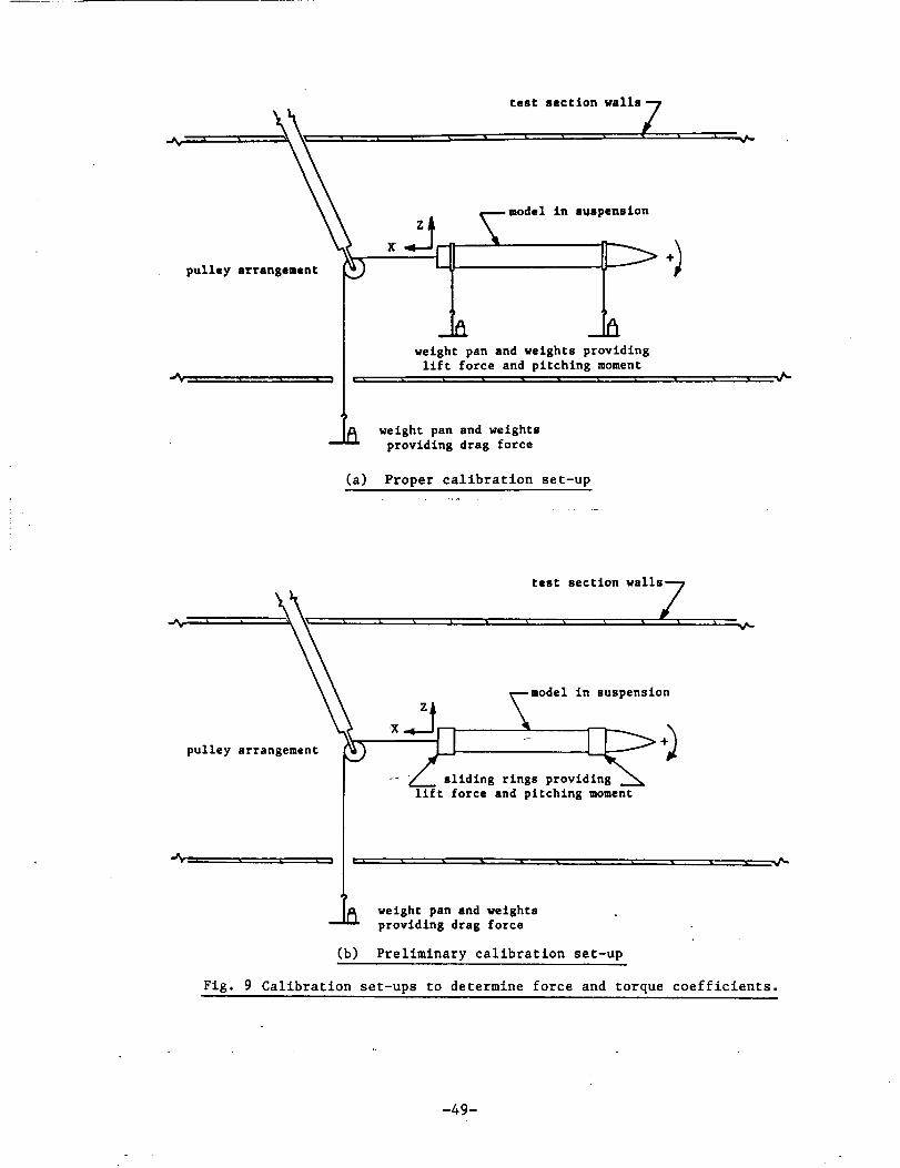
pulley arrangement

test section walls 7

model in suspenslon

weight pan and weights providinglift force and pitching moment

(a)

weight pan and weights

providing drag force

Proper calibration set-up

-- "_.... sliding rings providinglift force and pitching moment

)

weight pan and weightsproviding drag force

(b) Preliminary calibration set-up

Fig. 9 Calibration set-ups to determine force and torque coefficients.

-49-

4-===4

I.ousth

(a) Free stream conditions

I J J J J J J J J j

J

Boundmry Layer Growth

4---

4---

4---

LeajCh

a

(b) Flow with boundaries.

Fig. I0 Buoyancy effects in a closed throat wind tunnel.

-50-

!

)

I

!

n/b

! |

o

T

fl

Vi

0

"11z

- g

p

I

.-I

X

0

o

o

0

m

uo

-51-

f

m

4J w

.,-4_J

0.i-I

W

W

D.I

0

U0

I.."1

"1

O'I

t_

v

,1.1

0

1.1

0

U

0

_M

-52-

(a) Unconfined flow

\ \ \ \ \ \ \ \ \ \

•/ / / / / / / / / / /

(b) Confined flow

Fig. 13 Blockage effects in a closed throat wind tunnel.

-53-

(.1

r'l I> o

! II

1"3

1-11)0

!

_.Ua!D!J.J.O0_) 5DJC]

I

0U')

!0

4(-

6

L,_

..1:3

"00c">._GJ

0 n."U3

0

0

,,-I

WQJ

0

I11

0 Q'I

,,o

_o

U

-54-

.4

.3

c,¢_u

,m

0.2(J

o_o

C_

vo

vv vv. n

u _ u

50 1O0 1 0 200

Reynolds number (dia,lO "_ )

(a) Drag, 0 ° base, Run 001/003, free transition

I

25O

.2

"0E oo0

-.I

-,2

o

o

n

I_ Lift. Run 001

Pitching moment. Run 001

Lift. Run 003

Pitching moment. Run 003

[] ¢ []o Q

...... ;,..... - ............

¢v v

0

Fig. 15

! 1 _ I 150 100 1 0 200 250

Reynolds number (dia*10"3)

(b) Lift and pitching moment, 0 ° base,Run 001/003, free transition

MSBS drag, llft, and pitching moment results.

-55-

.4-

.3

c-

+m

(3%=L0--

_.20

8r_

O !o s'o ;oo '200

Reynolds number (dia..lO -'_)

(c) Drag, 0 ° base, Run 006, free transition

!

250

.2

n Uft jv Pitching moment

.1

¢- rl0 n O n On

•-_ o n o ooo

•- 0 ......................v '_.... ......_a- - -_'-_- _,-'-vvv_'.v-__, ....

-.I

-.2I I I | I

0 50 1O0 1.50 200 250

Reynolds number (die.,lO "_ )

o

(d) Lift and pitching moment, 0 ° base,

Run 006, free transition

Fig. 15 cont'd

-56-

.4-

.3

¢-,mut_

¢_.20C.)

O_oL.

C3

.1

[3

V v

rln 013

[]

J D Run 004 Iv Run 00,5

(e) Drag,

|

I00 150

Reynolds number (dio.,lO "_)

. i

200 250

0 ° base, Run 004/005, fixed transition

.2

t-

O

oC_

-.I

-.20

m Uft. Run 004

v Pitching moment, Run 004

o Lift. Run 005

4> Pitching moment, Run 005

v o

v v #q o o n o............o o v o _l

-_- o--_.-- _-- _-v--v.-_ ...............

m0

[]

l i i i •

50 1O0 150 200 250

Reynolds number (dia., 10 -3 )

(f) Lift and pitching moment, 0 ° base,

Run 004/005, fixed transition

Fig. 15 cont'd

-57-

.4-

.3

"E

(J

0.20

0t,.

C_

.1

0

(g)

J i o !I00 150 200 250

Reynolds number (dio.,lO -_ )

Drag, 30 ° base, Run 302, free transition

.4

_.2

oO

.I

0

0

I O Lift lv Pitchin 9 moment

Oi:]

V

i I I !

50 1O0 150 200

Reynolds number (dio., 1 0 -_)

250

(h) Lift and pitching moment, 30 ° base,

Run 302, free transition

Fig. 15 cont'd

-58-

.4

.3

4.a¢-

u

Wp-QJ0.2

0

oL

.1

0

0

(i)

n

D

i i ! i

50 100 150 200

Reynolds number (dia.,lO -_)

Drag, 40 ° base, Run 401, free transition

2;o

.4-

.3-

U_=.2-

0(J

,1

n Lift Iv Pitching moment

D

n0

-o--d-.- D_n

n0 D

v v

50 100 1 0 2 0 250

Reynolds number (dio.,lO "z )

(j) Lift and pitching moment, 40 ° base,

Run 401, free transition

Fig. 15 cont'd

-59-

.B

.6

c-

.o

_.4.(D

_noL=

c_

.2

00

I= = J

=°I

' 6o ' '50 I 150 200

Reynolds number (dio.,lO -3 )

(k) Drag, 45 ° base, Run 451/453, free transition

!

250

1.2 Lift1.2 Pitching moment

.8

c-

U

o_D

,4

.2 Q D

1

• Bin •

• I .8IIj I - hol) i otho) .s#

n

rn

.2

0

0 100

(i)

• I

0

0 50

Reynolds number (dia.,1 0 .3 )

Lift and pitching moment, 45 ° base,Run 451/453, free transition

i

100

Fig. 15 cont'd

-60-

.8

.6

4)u

0.4C.)

0k.

C3

.2

[] oo

[]

Reynolds number (dio.,10 °_ )

(m) Drag, 45 ° base, Run 454, fixed transition

!

250

1.2

.8

U

.6

0t)

.4

.2"

0

0

13 Lift. 1' L,=

• Lift,_ N,D

V Pitching moment. _ x-o

• Pitching moment. _ =-u

13 n

o

v- ,_______-_- _-_-v-v

I 0 # m g '_1O0 150 200 250

Reynolds number (dio.,lO -_ )

(n) Lift and pitching moment, 45 ° base,

Run 454, fixed transition

Fig. 15 cont'd

-61-

.6

.4_

m'U

0.4

D6

,2

gl

D

DI:1

D

0 100 1 0 200

Reynolds number (dio.,1 0 -_)

(o) Drag, 50 ° base, Run 501, free transition

!

250

t.2

.9

¢-q3u

qJ0

r_

.3

0

o []

[] _]D

1_ LiftPitchin 9 moment

! i i i i

50 1O0 150 200 250

Reynolds number (dio.,10 -3)

(p) Lift and pitching moment, 50 ° base,

Run 501, free transition

Flg. 15 cont'd

-62-

region of minimum pressure

.6.

Q),wu

om

wP-

o

o

.2

F o

o

oI::1

o o o---°'o

0

0 100 150 2 0

Reynolds number (dio.* 10 -z )

(q) Drag, 60 ° base, Run 601, free transition

|

250

1.2"

.8

,mu,m .6 -

¢)

o

.4

.2-

00

o o__°__o

/o o

o/[]

v o\ v ....

Lift Iv Pitching moment

i i i i i

50 1O0 1SO 200 250

Reynolds number (dio.*l 0-_ )

(r) Lift and pitching moment, 60 ° base,

Run 601, free transition

Fig. 15 cont'd

-63-

! I !

f /J

0I

l

.o

n _ 0

I !

• •

lua!0!_Jaoo 5oJO

I

1l, 1l

!I!

0

0

0

0_t3

_o

<I:

o- E0

(./3

0

o

4J

:Io

-64-

1.2

.B.4-*C

u

.6-0

.n.4 =

I

=3 Freq, transition

Jv Fixed transition

I 0 20 30 40

Slant Angle (,_)

60 70

Fi_. 17 MSBS llft results.

1,2 "

I

,u

U

00

t-

.6Eo

c ,4r-

U

.m

O.

.2

I

a Free transition I

Iv Rxed tronsition

i i ! ! ! u

I 0 20 30 4O 50 60

Slr]nt Angle (_

Fig. 18 MSBS pitching moment results.

=

-65-

#

4,,,I

I=

o

,,l.,i

14

o

o

u_

"-66- ORIGINAL PAGE

BLACK AND WHITE Pt4OTOGRAPH

1.2

.8

0

O.t_

I

.4

.2

13 30 degree bale I

ORIGYNAE PAGE

8LACK AND WHITE PHOTOGRAPH

O w

o ._ .;_ ._ .; ,ZR/O.

2. Pressure distribution (30 ° base).

Fig. 20a Flow visualization on the 30 = base (Liquid crystals).

-67-

I. Vortical flow pattern (50 = base).

l,i

- |

.8

0

0

.6,

o.UI

,4-

0

.I

$0o

o ._, ._ .i_ .6 ;2i_/o

2. Pressure distribution (50 ° base).

Fig. 20b Flow visualization on 50° base (Liquid crystals).

-68- ORIGINAL PAGE

BLACK AND WHITE PHOTOGRAPH

.I

-.4 | , , , , l

Transition (VSAERO) Transition (SANDRAG)

,II

x/L

Fig. 21 Pressure distribution (VSAERO) and predicted

transition locations (0° base).

.3

_.2

u

OU

cnO

oo

Laminar

boundary layer_k

Transition

moving forward

j Roughness-|_m

1../Roughneaa-[_

Pressure _d. ra_.a____

Skin friction,

-x---

Base Dra$

lOO 200 300 4 o

Reynolds Number (dio., ,10 -3)

!

500

Fig. 22 Details of SANDRAG computations.

-69-

!

0

n-

O n

I !

lua! !LlaOD 5oJC]

|

0-ur_

IN

C)0

I0

0 "

o Z0,,- if)

"10!

0C

n-

oif')

0

0

I.M

0

-70-

II nNh

ig. -olm£

"l

p,

INk.

Jl,2

I 2J2222

*_l '

Fig. 24 Schematic of pressure telemetry system.

Cable

• LOS D/a

Ven¢ Tuba J

0.5

< 10-32' _Sread . h i

n Face•152_,,

Fig. 25 Details of pressure transducer.

-71-

\

?.

0

v

0

1-

,-4

0

-72-

o

o

\

AI

I-ell

! !

\

0

!

/

I s

I '/,

P

-73-

r--

m

b_0

1

odci

g'l

v

0

-74-

I.IU.I.I

G,=&l

4.1

0 0

0 >v-I

U Iiim _C _

O"m

III Ill

ol01

•r-r'r'l I

L11, I,I I

I

OI

OI

'._1 0m U

V

lillll i11_

U

m m

4.1

0

m

0

m

U

U

=

4.a

r_e

¢,1m

-75-

25

2O

O 1504

I)1

UC: 10

\ [] ,--88.6V T- 84.4 ;

__ ,_--7_8.1 F

A

0 2 4 6 8

Frequency (kHz)

,'o

Fig. 28 Pressure transducer calibration curves.

10,

8

"W"1"•e 6'

UCG)

O" 4"

t.b-

/

/

/

QI -/. v _ .':" :

I

_uG a

:ERATING RANGE

v i v v

ll T= 78.7 FV T= 91.3 F

O

Volts

Fig. 29 Effects of input voltage on output frequency.

-76-

0

i,n

D b 0

! ! !

II

III

IIIIII

I

(gsoq) do-

!

O0i

tip

0

0

n

n,,-L"N

,1=1

c_

1,4!

I,.4

,,..io

o ,,-I

tm

oo'3

-77-

! ! ! I I

II

!

(aSDEI) do-

C)

C)

tm

c,,,i

-I

o

o

,.a

-78-

£:<x._ceAO'rw',,sl_o'_

1. Report No.

NASA CR-181708

4. T'cle and Subtitle

Report Documentation Page

2. Government Accession No. 3. Recipient's Catalog No.

5. Report Date

An Experimental Investigation of the AerodynamicCharacteristics of Slanted Base Ogive Cylinders UsingMagnetic Suspension Technology

7. Author(s)

Charles W. Alcorn

November 1988

6. Performing Organization Code

8. Performing Organization Report No.

10. Work Unit No.

505-61-91-039. Performing Organization Name and Address

Old Dominion University II.

Department of Mechanical Engineering and Mechanics

Norfolk, VA 23508 13.

12. Sponsoring Agency Name and Address

National Aeronautics and Space AdministrationLangley Research CenterHampton, VA 23665-5225

Contract or Grant No.

NAGI-716

Type of Report and Period Covered

Contractor Report

14. Sponsoring Agency Code

15. Supplementary Notes

This report was originally submitted to Old Dominion University in partial fulfillment ofthe requirements for the degree of Master of Science. Thesis advisor and PrincipalInvestigator was Dr. Colin P. Britcher.

Langley Technical Monitor: Richmond P. BoydenProgress Report for the period April I, 1988 through September 30, 1988.

16. Abstract

An experimental investigation is reported on slanted base ogive cylinders at zero incidence.The Mach number range is 0.05 to 0.3. All flow disturbances associated with wind tunnelsupports are eliminated in this investigation by magnetically suspending the wind tunnelmodels. The sudden and drastic changes in the lift, pitching moment, and drag for a slightchange in base slant angle are reported. Flow visualization with liquid crystals and oil isused to observe base flow patterns, which are responsible for the sudden changes inaerodynamic characteristics. Hysteretic effects in base flow pattern changes are present inthis investigation and are reported. The effect • of a wire support attachment on the 0 °

slanted base model is studied. Computational drag and transition location results usingVSAERO and SANDRAG are presented and compared with experimental results. Basepressure measurements over the slanted bases are made with an onboard pressure

transducer using remote data telemetry.

17. Key Words (Suggested by Author(s))

Magnetic Suspension and Balance SystemOgive CylindersWakes

19. Security Ctassif. (of this report)

Unclassified

NASA FORM 1626 OCT 86

18. Distribution Statement

Unclassified - Unlimited

Subject category - 02, 09

20. Security Classif. (of this page)

Unclassified

21..No. of pages

89

22. Price

A05