vol. i - smarandache notions journal - university of new mexico
TRANSCRIPT
FLORENTIN SMARANDACHE
COLLECTED PAPERS, VOL. I (SECOND EDITION)
Translated from Romanian and French
'1
'1 11
n i s t nij j i i s
i j i s iij j i i s t
M A M AM A M A
+ + −+
= = + =+ + +
=∏ ∏ ∏
ILQ
2007
1
Collected Papers, Vol. 1
(first edition 1996, second edition 2007)
Translated from Romanian and French into English
Florentin Smarandache, Ph D
Chair of Department of Mathematics & Sciences University of New Mexico, Gallup, USA
ILQ
2007
2
This book can be ordered in a paper bound reprint from: Books on Demand ProQuest Information & Learning (University of Microfilm International) 300 N. Zeeb Road P.O. Box 1346, Ann Arbor MI 48106-1346, USA Tel.: 1-800-521-0600 (Customer Service)
http://wwwlib.umi.com/bod/basic Copyright 2007 by InfoLearnQuest (Ann Arbor) and the Author Many books can be downloaded from the following Digital Library of Science: http://www.gallup.unm.edu/~smarandache/eBooks-otherformats.htm Peer Reviewers: Prof. Mihaly Bencze, Department of Mathematics, Áprily Lajos College, Bra ov, Romania.
Dr. Sukanto Bhattacharya, Department of Business Administration, Alaska Pacific University, U.S.A. Prof. Dr. Adel Helmy Phillips. Ain Shams University, 1 El-Sarayat st., Abbasia, 11517, Cairo, Egypt. (ISBN-10): 1-59973-048-0 (ISBN-13): 978-1-59973-048-6 (EAN): 9781599730486 Printed in the United States of America
3
COLLECTED PAPERS1
(VOL. I, second edition)
(Articles, notes, generalizations, paradoxes, miscellaneous in
Mathematics, Linguistics, and Education)
1Some papers not included in the volume were confiscated by the Secret Police in September 1988, when the author left Romania. He spent 19 months in a Turkish political refugee camp, and immigrated to the United States in March 1990. Despite the efforts of his friends, the papers were not recovered.
4
CONTENTS
CONTENTS 4
A NUMERICAL FUNCTION IN CONGRUENCE THEORY 7
A GENERAL THEOREM FOR THE CHARACTERIZATION OF N PRIME NUMBERS SIMULTANEOUSLY 11
A METHOD TO SOLVE THE DIOPHANTINE EQUATION ax2 − by2 + c = 0 16
SOME STATIONARY SEQUENCES 22
ON CARMICHAËL’S CONJECTURE 24
A PROPERTY FOR A COUNTEREXAMPLE TO CARMICHAËL’S CONJECTURE 27
ON DIOPHANTINE EQUATION X 2 = 2Y 4 − 1 29
ON AN ERDÖS’ OPEN PROBLEMS 31
ON ANOTHER ERDÖS’ OPEN PROBLEM 33
METHODS FOR SOLVING LETTER SERIES 34
GENERALIZATION OF AN ER’S MATRIX METHOD FOR COMPUTING 36
ON A THEOREM OF WILSON 38
A METHOD OF RESOLVING IN INTEGER NUMBERS OF CERTAIN NONLINEAR EQUATIONS 43
A GENERALIZATION REGARDING THE EXTREMES OF A TRIGONOMETRIQUE FUNCTION 45
ON SOLVING HOMOGENE SYSTEMS 47
5
ABOUT SOME PROGRESSIONS 49
ON SOLVING GENERAL LINEAR EQUATIONS IN THE SET OF NATURAL NUMBERS 51
EXISTENCE AND NUMBER OF SOLUTIONS OF DIOPHANTINE QUADRATIC
EQUATIONS WITH TWO UNKNOWNS IN Z AND N 55
CONVERGENCE OF A FAMILY OF SERIES 57
ALGORITHMS FOR SOLVING LINEAR CONGRUENCES AND SYSTEMS OF LINEAR CONGRUENCES 61
BASES OF SOLUTIONS FOR LINEAR CONGRUENCES 69
CRITERIA OF PRIMALITY 74
INTEGER ALGORITHMS TO SOLVE DIOPHANTINE LINEAR EQUATIONS AND SYSTEMS 78
A METHOD TO GENERALIZE BY RECURRENCE OF SOME KNOWN RESULTS 135
A GENERALIZATION OF THE INEQUALITY OF HÖLDER 136
A GENERALIZATION OF THE INEQUALITY OF MINKOWSKI 138
A GENERALIZATION OF AN INEQUALITY OF TCHEBYCHEV 139
A GENERALIZATION OF EULER’S THEOREM 140
A GENERALIZATION OF THE INEQUALITY CAUCHY-BOUNIAKOVSKI-SCHWARZ 147
GENERALIZATIONS OF THE THEOREM OF CEVA 149
AN APPLICATION OF THE GENERALIZATION OF CEVA’S THEOREM 153
A GENERALIZATION OF A THEOREM OF CARNOT 156
6
SOME PROPERTIES OF NEDIANES 158
GENERALIZATIONS OF DEGARGUES THEOREM* 160
K-NOMIAL COEFFICIENTS 161
A CLASS OF RECURSIVE SETS 165
A GENERALIZATION IN SPACE OF JUNG’S THEOREM 172
MATHEMATICAL RESEARCH AND NATIONAL EDUCATION 174
JUBILEE OF “GAMMA” JOURNAL 177
HAPPY NEW MATHEMATICAL YEARS! 179
DEDUCIBILITY THEOREMS IN BOOLEAN LOGIC 180
LINGUISTIC-MATHEMATICAL STATISTICS IN RECENT ROMANIAN POETRY 184
A MATHEMATICAL LINGUISTIC APPROACH TO REBUS 192
HYPOTHESIS ON THE DETERMINATION OF A RULE FOR THE CROSS WORDS PUZZLES 202
THE LANGUAGE OF SPIRITUAL REBUS DEFINITIONS 204
THE LETTERS’ FREQUENCY (BY EQUAL GROUPS) IN THE ROMANIAN JURIDICAL TEXTS 210
MATHEMATICAL FANCIES AND PARADOXES 212
7
A NUMERICAL FUNCTION IN CONGRUENCE THEORY
In this article we define a function L which will allow us to generalize (separately or simultaneously) some theorems from Numbers Theory obtained by Wilson, Fermat, Euler, Gauss, Lagrange, Leibnitz, Moser, Sierpinski.
§1. Let A be the set { , 2m m p pβ β∈ = ± ±Z with p an odd prime, *Nβ ∈ , or
m = ±2α with α = 0,1,2 , or }0m = .
Let’s consider m = ε p1α1 ...ps
α s , with ε = ±1 , all *i Nα ∈ , and p1,..., ps distinct
positive numbers. We construct the FUNCTION L : Z → Z ,
L(x, m) = (x + c1)...(x + cϕ (m ) ) where c1,...,cϕ (m ) are all residues modulo m relatively prime to m , and ϕ is the Euler’s function. If all distinct primes which divide x and m simultaneously are pi1
...pirthen:
L(x, m) ≡ ±1(mod pi1
αi1 ...pir
α ir ) , when m ∈A respective by m ∉A , and
L(x, m) ≡ 0(mod m / (pi1
α i1 ...pir
α ir )) .
Noting d = pi1
α i1 ...pir
α ir and m ' = m / d we find:
L(x, m) ≡ ±1 + k10d ≡ k2
0m '(mod m) where k1
0 , k20 constitute a particular integer solution of the Diophantine equation
k2m '− k1d = ±1 (the signs are chosen in accordance with the affiliation of m to A ). This result generalizes the Gauss’ theorem (c1,...,cϕ (m ) ≡ ±1(mod m)) when m ∈A
respectively m ∉A (see [1]) which generalized in its turn the Wilson’s theorem (if p is prime then ( p − 1)! ≡ −1(mod m) ). Proof.
The following two lemmas are trivial: Lemma 1. If c1,...,cϕ ( pα )
are all residues modulo pα relatively prime to pα , with
p an integer and *Nα ∈ , then for k ∈Z and *Nβ ∈ we have also that
1 ( ),...,
pkp c kp c α
β βϕ
+ + constitute all residues modulo pα relatively prime to it is
sufficient to prove that for 1 ≤ i ≤ ϕ(pα ) we have that kpβ + ci is relatively prime to pα , but this is obvious. Lemma 2. If c1,...,cϕ (m ) are all residues modulo m relatively prime to m ,
iipα divides m and 1i
ipα + does not divide m , then c1,...,cϕ (m ) constitute ϕ(m / piα i )
systems of all residues modulo piαi relatively prime to pi
αi .
8
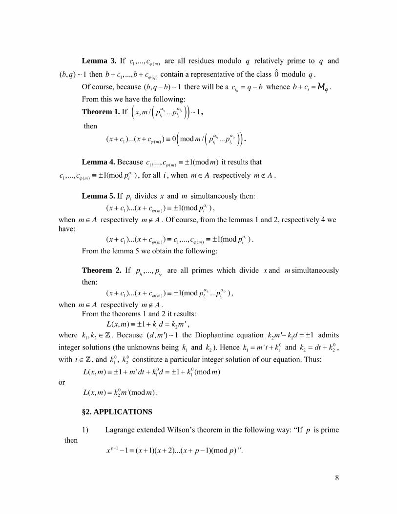
Lemma 3. If 1 ( ),..., mc cϕ are all residues modulo q relatively prime to q and
( , ) 1b q ∼ then b + c1,...,b + cϕ (q) contain a representative of the class 0̂ modulo q . Of course, because ( , ) 1b q b− ∼ there will be a ci0
= q − b whence b + ci = Mq .
From this we have the following: Theorem 1. If ( )( )1
1, / ... 1ii s
si ix m p pαα ∼ ,
then
( )( )1
11 ( )( )...( ) 0 mod / ...i ir
rm i ix c x c m p pα αϕ+ + ≡ .
Lemma 4. Because c1,...,cϕ (m ) ≡ ±1(mod m) it results that
c1,...,cϕ (m) ≡ ±1(mod piαi ) , for all i , when m ∈A respectively m ∉A .
Lemma 5. If pi divides x and m simultaneously then:
(x + c1)...(x + cϕ (m) ) ≡ ±1(mod piαi ) ,
when m ∈A respectively m ∉A . Of course, from the lemmas 1 and 2, respectively 4 we have:
(x + c1)...(x + cϕ (m) ) ≡ c1,...,cϕ (m) ≡ ±1(mod piαi ) .
From the lemma 5 we obtain the following: Theorem 2. If
1,...,
ri ip p are all primes which divide x and m simultaneously then:
(x + c1)...(x + cϕ (m ) ) ≡ ±1(mod pi1
αi1 ...pir
αir ) , when m ∈A respectively m ∉A .
From the theorems 1 and 2 it results: L(x,m) ≡ ±1 + k1 d = k2m ' ,
where k1, k2 ∈Z . Because ( , ') 1d m ∼ the Diophantine equation 2 1' 1k m k d− = ± admits integer solutions (the unknowns being 1k and 2k ). Hence 0
1 1'k m t k= + and k2 = dt + k20 ,
with t ∈Z , and 0 01 2, k k constitute a particular integer solution of our equation. Thus:
L(x, m) ≡ ±1 + m 'dt + k10d = ±1 + k1
0 (mod m) or
L(x, m) = k20m '(mod m) .
§2. APPLICATIONS 1) Lagrange extended Wilson’s theorem in the following way: “If p is prime
then 1 1 ( 1)( 2)...( 1)(mod )px x x x p p− − ≡ + + + − ”.
9
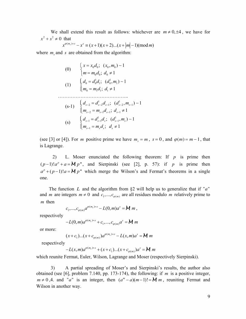
We shall extend this result as follows: whichever are m ≠ 0,±4 , we have for x2 + s2 ≠ 0 that
( ) ( 1)( 2)...( 1)(mod )sm s sx x x x x m mϕ + − ≡ + + + − where ms and s are obtained from the algorithm:
(0) 0 0 0 0
0 0 0
; ( , ) 1; 1
x x d x mm m d d
=⎧⎨ = ≠⎩
∼
(1) 1 1
0 0 1 0 1
0 1 1 1
; ( , ) 1; 1
d d d d mm m d d
⎧ =⎪⎨
= ≠⎪⎩
∼
……………………………………..
(s-1) 1 1
2 2 1 2 1
2 1 1 1
; ( , ) 1; 1
s s s s s
s s s s
d d d d mm m d d
− − − − −
− − − −
⎧ =⎪⎨
= ≠⎪⎩
∼
(s) 1 1
1 1 1
1
; ( , ) 1; 1
s s s s s
s s s s
d d d d mm m d d
− − −
−
⎧ =⎪⎨
= ≠⎪⎩
∼
(see [3] or [4]). For m positive prime we have ms = m , s = 0 , and ϕ(m) = m − 1 , that is Lagrange.
2) L. Moser enunciated the following theorem: If p is prime then ( 1)! ''pp a a p− + =M , and Sierpinski (see [2], p. 57): if p is prime then
( 1)! ''pa p a p+ − =M which merge the Wilson’s and Fermat’s theorems in a single one.
The function L and the algorithm from §2 will help us to generalize that if "a"
and m are integers m ≠ 0 and c1,...,cϕ (m ) are all residues modulo m relatively prime to m then
( )1 ( ),..., (0, ) sm s s
mc c a L m a mϕϕ
+ − =M , respectively
( )1 ( )(0, ) ,..., sm s s
mL m a c c a mϕϕ
+− + =M or more:
( )1 ( )( )...( ) ( , ) sm s s
mx c x c a L x m a mϕϕ
++ + − =M respectively
( )1 ( )( , ) ( )...( ) sm s s
mL x m a x c x c a mϕϕ
+− + + + =M which reunite Fermat, Euler, Wilson, Lagrange and Moser (respectively Sierpinski).
3) A partial spreading of Moser’s and Sierpinski’s results, the author also obtained (see [6], problem 7.140, pp. 173-174), the following: if m is a positive integer, m ≠ 0 ,4. and "a" is an integer, then ( )( 1)! ma a m m− − =M , reuniting Fermat and Wilson in another way.
10
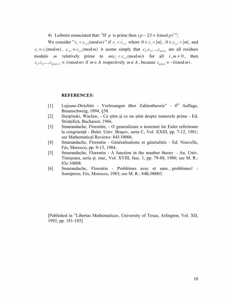
4) Leibnitz enunciated that: ”If p is prime then ( p − 2)! ≡ 1(mod p)"”; We consider ” ci < ci +1(mod m) ” if ci
' < ci+1' where 0 ≤ ci
' < m , 0 ≤ ci+1' < m , and
ci ≡ ci' (mod m) , ci+1 ≡ ci+1
' (mod m) it seems simply that c1,c2 ,...,cϕ (m ) are all residues modulo m relatively prime to m(ci < ci+1(mod m)) for all i , m ≠ 0 , then c1,c2 ,...,cϕ (m )−1 ≡ ±(mod m) if m ∈A respectively m ∉A , because cϕ (m ) ≡ −1(mod m) . REFERENCES:
[1] Lejeune-Dirichlet - Vorlesungen über Zahlentheorie” - 4te Auflage, Braunschweig, 1894, §38.
[2] Sierpinski, Waclaw, - Ce ştim şi ce nu ştim despre numerele prime - Ed. Stiinţifică, Bucharest, 1966.
[3] Smarandache, Florentin, - O generalizare a teoremei lui Euler referitoare la congruenţă - Bulet. Univ. Braşov, seria C, Vol. XXIII, pp. 7-12, 1981; see Mathematical Reviews: 84J:10006.
[4] Smarandache, Florentin - Généralisations et généralités - Ed. Nouvelle, Fés, Morocco, pp. 9-13, 1984.
[5] Smarandache, Florentin - A function in the number theory – An. Univ. Timişoara, seria şt. mat., Vol. XVIII, fasc. 1, pp. 79-88, 1980; see M. R.: 83c:10008.
[6] Smarandache, Florentin - Problèmes avec et sans…problèmes! - Somipress, Fés, Morocco, 1983; see M. R.: 84K:00003.
[Published in ”Libertas Mathematica», University of Texas, Arlington, Vol. XII, 1992, pp. 181-185]
11
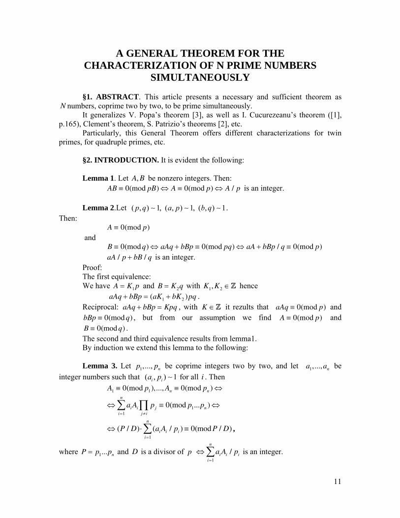
A GENERAL THEOREM FOR THE CHARACTERIZATION OF N PRIME NUMBERS
SIMULTANEOUSLY §1. ABSTRACT. This article presents a necessary and sufficient theorem as N numbers, coprime two by two, to be prime simultaneously. It generalizes V. Popa’s theorem [3], as well as I. Cucurezeanu’s theorem ([1], p.165), Clement’s theorem, S. Patrizio’s theorems [2], etc. Particularly, this General Theorem offers different characterizations for twin primes, for quadruple primes, etc. §2. INTRODUCTION. It is evident the following: Lemma 1. Let A, B be nonzero integers. Then:
AB ≡ 0(mod pB) ⇔ A ≡ 0(mod p) ⇔ A / p is an integer.
Lemma 2.Let ( , ) 1, ( , ) 1, ( , ) 1p q a p b q∼ ∼ ∼ . Then:
A ≡ 0(mod p) and
B ≡ 0(mod q) ⇔ aAq + bBp ≡ 0(mod pq) ⇔ aA + bBp / q ≡ 0(mod p) aA / p + bB / q is an integer.
Proof: The first equivalence:
We have A = K1 p and B = K2q with K1, K2 ∈Z hence aAq + bBp = (aK1 + bK2 )pq .
Reciprocal: aAq + bBp = Kpq , with K ∈Z it rezults that aAq ≡ 0(mod p) and bBp ≡ 0(mod q) , but from our assumption we find A ≡ 0(mod p) and B ≡ 0(mod q) . The second and third equivalence results from lemma1. By induction we extend this lemma to the following: Lemma 3. Let p1,..., pn be coprime integers two by two, and let a1,...,an be
integer numbers such that ( , ) 1i ia p ∼ for all i . Then A1 ≡ 0(mod p1),..., An ≡ 0(mod pn ) ⇔
⇔ ai Aii=1
n
∑ pjj ≠ i∏ ≡ 0(mod p1...pn ) ⇔
⇔ (P / D) ⋅ (aiAii=1
n
∑ / pi ) ≡ 0(mod P / D) ,
where P = p1...pn and D is a divisor of p ⇔ aiAii=1
n
∑ / pi is an integer.
12
§3. From this last lemma we can find immediately a GENERAL THEOREM: Let Pij ,1 ≤ i ≤ n,1 ≤ j ≤ mi , be coprime integers two by two, and let
r1,...,rn ,a1,...,an be integer numbers such that ai be coprime with ri for all i . The following conditions are considered: (i) pi
1,..., pin1
, are simultaneously prime if and only if ci ≡ 0(mod ri ) , for all i .
Then: The numbers pij ,1 ≤ i ≤ n,1 ≤ j ≤ mi , are simultaneously prime if and only if
(*) (R / D) (aicii=1
n
∑ / ri ) ≡ 0(mod R / D) ,
where P = rii=1
n
∏ and D is a divisor of R .
Remark:
Often in the conditions (i) the module ri is equal to pijj =1
mi
∏ , or to a divisor of it,
and in this case the relation of the General Theorem becomes:
(P / D) (aicii=1
n
∑ / pijj =1
mi
∏ ) ≡ 0(mod P / D)
where
,
, 1
in m
iji j
P p=
= ∏ and D is a divisor of P .
Corollaries: We easily obtain that our last relation is equivalent with:
(aicii=1
n
∑ (P / pijj =1
mi
∏ ) ≡ 0(mod P) ,
and
(aicii=1
n
∑ / pijj =1
mi
∏ ) is an integer,
etc. The imposed restrictions for the numbers pij from the General Theorem are very wide, because if there would be two uncoprime distinct numbers, then at least one from these would not be prime, hence the m1 + ... + mn numbers might not be prime. The General Theorem has many variants in accordance with the assigned values for the parameters a1,...,an and r1,...,rm , the parameter D , as well as in accordance with the congruences c1,...,cn which characterize either a prime number or many other prime numbers simultaneously. We can start from the theorems (conditions ci ) which
13
characterize a single prime number (see Wilson, Leibnitz, F. Smarandache [4], or Siminov ( p is prime if and only if (p − k)!(k − 1)!− (−1)k ≡ 0(mod p) , when p ≥ k ≥ 1 ; here, it is preferable to take k = [( p + 1) / 2] , where [x] represents the gratest integer number ≤ x , in order that the number ( p − k)!(k − 1)! be the smallest possibly) for obtaining, by means of the General Theorem, conditions cj
' , which characterize many
prime numbers simultaneously. Afterwards, from the conditions ci ,cj' , using the General
Theorem again, we find new conditions ch" which characterize prime numbers
simultaneously. And this method can be continued analogically. Remarks Let mi = 1 and ci represent the Simionov’s theorem for all i
(a) If D = 1 it results in V. Popa’s theorem, which generalizes in the Cucurezeanu’s theorem and the last one generalizes in its turn Clement’s theorem!
(b) If D = P / p2 and choosing convenintly the parameters ai , ki for i = 1,2,3 , it results in S. Patrizio’s theorem.
Several Examples:
1. Let p1, p2 ,..., pn be positive integers >1, coprime integers two by two, and 1 ≤ ki ≤ pi for all i . Then p1, p2 ,..., pn are simultaneously prime if and only if:
(T) (pi − ki )!(ki − 1)!− (−1)ki⎡⎣ ⎤⎦i=1
n
∑ ⋅ pij ≠ i∏ ≡ 0(mod p1 p2 ...pn )
or
(U) (pi − ki )!(ki − 1)!− (−1)ki⎡⎣ ⎤⎦i=1
n
∑ ⋅ pij ≠ i∏ / (ps+1...pn ) ≡ 0(mod p1...ps )
or
(V) (pi − ki )!(ki − 1)!− (−1)ki⎡⎣ ⎤⎦i=1
n
∑ ⋅ pj / pi ≡ 0(mod pj )
or
(W) (pi − ki )!(ki − 1)!− (−1)ki⎡⎣ ⎤⎦i=1
n
∑ ⋅ pj / pi is an integer.
2. Another relation example (using the first theorem form [4]: p is a prime
positive integer if and only if (p − 3)!− (p − 1) / 2 ≡ 0(mod p)
(pi − 3)!− (pi − 1) / 2[ ]i=1
n
∑ ⋅ p1 / pi ≡ 0(mod p1)
14
3. The odd numbers … and … are twin prime if and only if: ( p − 1)!(3p + 2) + 2 p + 2 ≡ 0(mod p( p + 2)) or ( p − 1)!( p + 2) − 2 ≡ 0(mod p( p + 2)) or (p − 1)!+ 1[ ]/ p + (p − 1)!2 + 1[ ]/ (p + 2) is an integer.
These twin prime characterzations differ from Clement’s theorem (( p − 1)!4 + p + 4 ≡ 0(mod p( p + 2)))
4. Let ( , ) 1p p k+ ∼ then: p and p + k are prime simultaneously if and only if
( p − 1)!( p + k) + (p + k − 1)! p + 2 p + k ≡ 0(mod p(p + k)) , which differs from I. Cucurezeanu’s theorem ([1], p. 165):
k ⋅ k! (p − 1)!+ 1[ ]+ K !− (−1)k⎡⎣ ⎤⎦ p ≡ 0(mod p(p + k))
5. Look at a characterization of a quadruple of primes for p, p + 2, p + 6, p + 8 : (p − 1)!+ 1[ ]/ p + (p − 1)!2!+ 1[ ]/ (p + 2) + (p − 1)!6!+ 1[ ]/ (p + 6) + (p − 1)!8!+ 1[ ]/ (p + 8)
be an integer.
6. For 2, , 4p p p− + coprime integers tw by two, we find the relation: (p − 1)!+ p (p − 3)!+ 1[ ]/ (p − 2) + p (p + 3)!+ 1[ ]/ (p + 4) ≡ −1(mod p) ,
which differ from S. Patrizio’s theorem 8 (p + 3)!/ (p + 4)[ ]+ 4 (p − 3)!/ (p − 2)[ ]≡ −11(mod p)( ).
References
[1] Cucuruzeanu, I – Probleme de aritmetică şi teoria numerelor, Ed. Tehnică,
Bucharest, 1966. [2] Patrizio, Serafino – Generalizzazione del teorema di Wilson alle terne
prime - Enseignement Math., Vol. 22(2), nr. 3-4, pp. 175-184, 1976. [3] Popa, Valeriu – Asupra unor generalizări ale teoremei lui Clement - Studii
şi Cercetări Matematice, Vol. 24, nr. 9, pp. 1435-1440, 1972. [4] Smarandache, Florentin – Criterii ca un număr natural să fie prim - Gazeta
Matematică, nr. 2, pp. 49-52; 1981; see Mathematical Reviews (USA): 83a:10007.
15
[Presented at the 15th American Romanian Academy Annual Convention, which was held in Montréal, Québec, Canada, from June 14-18, 1990, at École Polytechnique de Montréal. Published in ”Libertas Mathemaica”, University of Texas, Alington, Vol. XI, 1991, pp. 151-5]
16
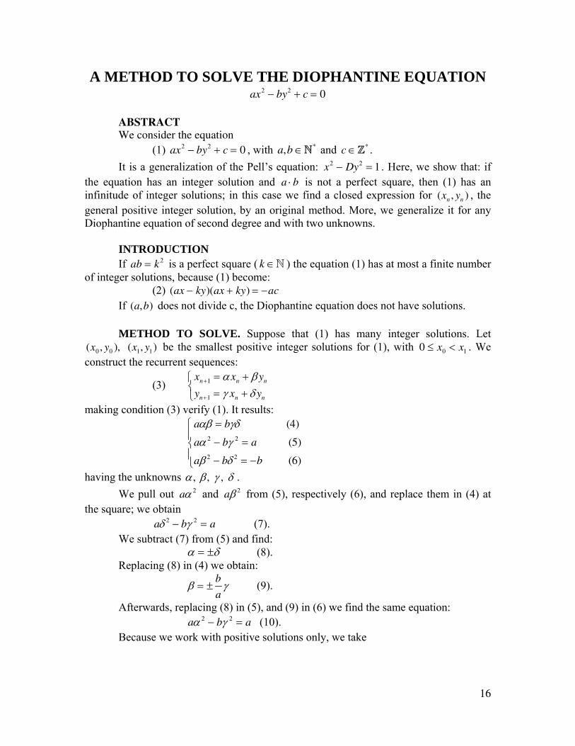
A METHOD TO SOLVE THE DIOPHANTINE EQUATION ax2 − by2 + c = 0
ABSTRACT We consider the equation (1) ax2 − by2 + c = 0 , with a,b ∈N* and c ∈Z* . It is a generalization of the Pell’s equation: x2 − Dy2 = 1 . Here, we show that: if the equation has an integer solution and a ⋅ b is not a perfect square, then (1) has an infinitude of integer solutions; in this case we find a closed expression for (xn , yn ) , the general positive integer solution, by an original method. More, we generalize it for any Diophantine equation of second degree and with two unknowns. INTRODUCTION If ab = k 2 is a perfect square ( k ∈N ) the equation (1) has at most a finite number of integer solutions, because (1) become: (2) (ax − ky)(ax + ky) = −ac If (a,b) does not divide c, the Diophantine equation does not have solutions. METHOD TO SOLVE. Suppose that (1) has many integer solutions. Let (x0 , y0 ), (x1, y1) be the smallest positive integer solutions for (1), with 0 ≤ x0 < x1 . We construct the recurrent sequences:
(3) xn+1 = α xn + βyn
yn+1 = γ xn + δ yn
⎧⎨⎩
making condition (3) verify (1). It results: aαβ = bγδ (4)
aα 2 − bγ 2 = a (5)
aβ 2 − bδ 2 = −b (6)
⎧
⎨⎪
⎩⎪
having the unknowns α , β, γ , δ . We pull out aα 2 and aβ 2 from (5), respectively (6), and replace them in (4) at the square; we obtain
aδ 2 − bγ 2 = a (7). We subtract (7) from (5) and find: α = ±δ (8). Replacing (8) in (4) we obtain:
β = ±b
aγ (9).
Afterwards, replacing (8) in (5), and (9) in (6) we find the same equation: aα 2 − bγ 2 = a (10). Because we work with positive solutions only, we take
17
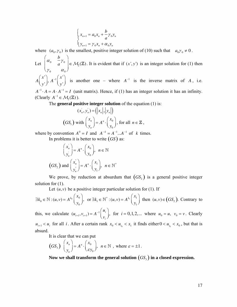
xn+1 = a0xn +
b
aγ 0yn
yn+1 = γ 0xn + α0yn
⎧⎨⎪
⎩⎪
where (a0 ,γ 0 ) is the smallest, positive integer solution of (10) such that a0γ 0 ≠ 0 .
Let
α0 b
aγ 0
γ 0 α0
⎛
⎝⎜⎜
⎞
⎠⎟⎟
∈M2 (Z) . It is evident that if (x ', y ') is an integer solution for (1) then
Ax '
y '
⎛⎝⎜
⎞⎠⎟
, A−1 x '
y '
⎛⎝⎜
⎞⎠⎟
is another one – where A−1 is the inverse matrix of A , i.e.
A−1 ⋅ A = A ⋅ A−1 = I (unit matrix). Hence, if (1) has an integer solution it has an infinity. (Clearly A
−1 ∈M2 (Z) ). The general positive integer solution of the equation (1) is:
( )' '( , ) ,n n n nx y x y=
GS1( ) with xn
yn
⎛⎝⎜
⎞⎠⎟
= An ⋅x0
y0
⎛⎝⎜
⎞⎠⎟
, for all n ∈Z ,
where by convention A0 = I and A− k = A−1...A−1 of k times. In problems it is better to write GS( ) as:
xn'
yn'
⎛
⎝⎜⎞
⎠⎟= An ⋅
x0
y0
⎛⎝⎜
⎞⎠⎟
, n ∈N
GS2( ) and
xn"
yn"
⎛
⎝⎜⎞
⎠⎟= An ⋅
x1
y1
⎛⎝⎜
⎞⎠⎟
, n ∈N*
We prove, by reduction at absurdum that GS2( ) is a general positive integer solution for (1). Let (u,v) be a positive integer particular solution for (1). If
∃k0 ∈N : (u,v) = Ak0
x0
y0
⎛⎝⎜
⎞⎠⎟
, or ∃k1 ∈N* : (u,v) = Ak1x1
y1
⎛⎝⎜
⎞⎠⎟
then (u,v) ∈ GS2( ). Contrary to
this, we calculate (ui+1,vi+1) = A−1 ui
vi
⎛⎝⎜
⎞⎠⎟
, for i = 0,1,2,... where u0 = u, v0 = v . Clearly
ui+1 < ui for all i . After a certain rank x0 < ui0< x1 it finds either 0 < ui0
< x0 , but that is absurd. It is clear that we can put
GS3( )
xn
yn
⎛
⎝⎜⎞
⎠⎟= An ⋅
x0
εy0
⎛⎝⎜
⎞⎠⎟
, n ∈N , where ε = ±1 .
Now we shall transform the general solution GS3( ) in a closed expression.
18
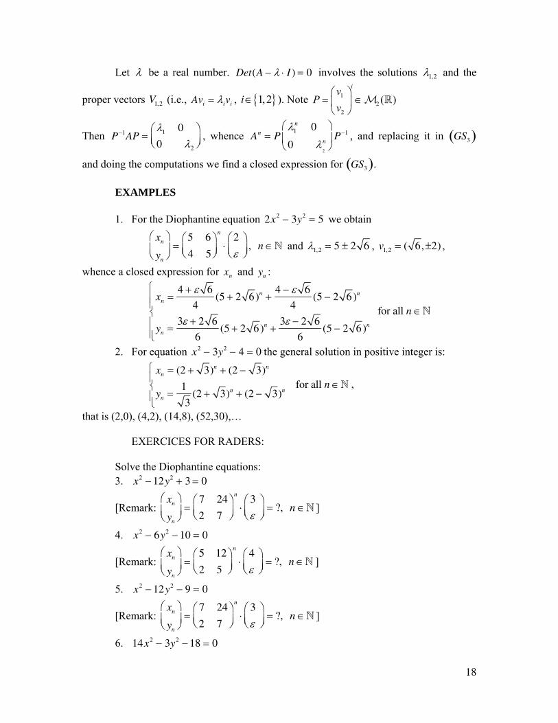
Let λ be a real number. Det(A − λ ⋅ I ) = 0 involves the solutions λ1,2 and the
proper vectors V1,2 (i.e., Avi = λivi , { }1,2i ∈ ). Note 12
2
( )iv
Pv
⎛ ⎞= ∈⎜ ⎟
⎝ ⎠M
Then P−1AP =λ1 0
0 λ2
⎛⎝⎜
⎞⎠⎟
, whence An = Pλ1
n 0
0 λ2
n
⎛
⎝⎜
⎞
⎠⎟ P−1 , and replacing it in GS3( )
and doing the computations we find a closed expression for GS3( ). EXAMPLES
1. For the Diophantine equation 2x2 − 3y2 = 5 we obtain
xn
yn
⎛
⎝⎜⎞
⎠⎟=
5 6
4 5
⎛⎝⎜
⎞⎠⎟
n
⋅2
ε⎛⎝⎜
⎞⎠⎟
, n ∈N and λ1,2 = 5 ± 2 6 , v1,2 = ( 6, ±2) ,
whence a closed expression for xn and yn :
xn =4 + ε 6
4(5 + 2 6)n +
4 − ε 6
4(5 − 2 6)n
yn =3ε + 2 6
6(5 + 2 6)n +
3ε − 2 6
6(5 − 2 6)n
⎧
⎨⎪⎪
⎩⎪⎪
for all n ∈N
2. For equation x2 − 3y2 − 4 = 0 the general solution in positive integer is:
xn = (2 + 3)n + (2 − 3)n
yn =1
3(2 + 3)n + (2 − 3)n
⎧
⎨⎪
⎩⎪
for all n ∈N ,
that is (2,0), (4,2), (14,8), (52,30),…
EXERCICES FOR RADERS:
Solve the Diophantine equations: 3. x2 − 12y2 + 3 = 0
[Remark:
xn
yn
⎛
⎝⎜⎞
⎠⎟=
7 24
2 7
⎛⎝⎜
⎞⎠⎟
n
⋅3
ε⎛⎝⎜
⎞⎠⎟
= ?, n ∈N ]
4. x2 − 6y2 − 10 = 0
[Remark:
xn
yn
⎛
⎝⎜⎞
⎠⎟=
5 12
2 5
⎛⎝⎜
⎞⎠⎟
n
⋅4
ε⎛⎝⎜
⎞⎠⎟
= ?, n ∈N ]
5. x2 − 12y2 − 9 = 0
[Remark:
xn
yn
⎛
⎝⎜⎞
⎠⎟=
7 24
2 7
⎛⎝⎜
⎞⎠⎟
n
⋅3
ε⎛⎝⎜
⎞⎠⎟
= ?, n ∈N ]
6. 14x2 − 3y2 − 18 = 0
19
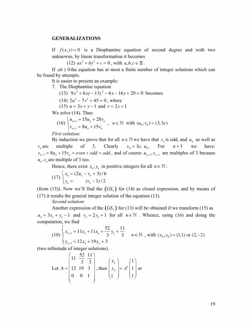
GENERALIZATIONS If f (x, y) = 0 is a Diophantine equation of second degree and with two unknowns, by linear transformation it becomes
(12) ax2 + by2 + c = 0 , with a,b,c ∈Z . If ab ≥ 0 the equation has at most a finite number of integer solutions which can
be found by attempts. It is easier to present an example: 7. The Diophantine equation
(13) 9x2 + 6xy − 13y2 − 6x − 16y + 20 = 0 becomes (14) 2u2 − 7v2 + 45 = 0 , where (15) u = 3x + y − 1 and v = 2y + 1
We solve (14). Thus:
(16)
un+1 = 15un + 28vn
vn+1 = 8un + 15vn
⎧⎨⎩
, n ∈N with (u0 ,v0 ) = (3, 3ε )
First solution: By induction we prove that for all n ∈N we have that vn is odd, and un as well as
vn are multiple of 3. Clearly v0 = 3ε, u0 . For n + 1 we have: vn+1 = 8un + 15vn = even + odd = odd , and of course un+1,vn+1 are multiples of 3 because un ,vn are multiple of 3 too.
Hence, there exist xn , yn in positive integers for all n ∈N :
(17) xn = (2un − vn + 3) / 6
yn = (vn − 1) / 2
⎧⎨⎩
(from (15)). Now we’ll find the GS3( ) for (14) as closed expression, and by means of (17) it results the general integer solution of the equation (13). Second solution:
Another expression of the GS3( ) for (13) will be obtained if we transform (15) as un = 3xn + yn − 1 and vn = 2yn + 1 for all n ∈N . Whence, using (16) and doing the computation, we find
(18) xn+1 = 11xn + 11xn +
52
3yn +
11
3yn+1 = 12xn + 19yn + 3
⎧⎨⎪
⎩⎪ n ∈N , with (x0 , y0 ) = (1,1) or (2,−2)
(two infinitude of integer solutions).
Let A =
11 52
3 11
312 19 3
0 0 1
⎛
⎝
⎜⎜⎜⎜⎜
⎞
⎠
⎟⎟⎟⎟⎟
, then 1111
nn
n
xy A
⎛ ⎞ ⎛ ⎞⎜ ⎟ ⎜ ⎟=⎜ ⎟ ⎜ ⎟
⎜ ⎟⎜ ⎟ ⎝ ⎠⎝ ⎠
or
20
(19) 22
11
nn
n
xy A
⎛ ⎞ ⎛ ⎞⎜ ⎟ ⎜ ⎟= −⎜ ⎟ ⎜ ⎟
⎜ ⎟⎜ ⎟ ⎝ ⎠⎝ ⎠
, always n ∈N .
From (18) we have always 1 0... 1(mod 3)n ny y y+ ≡ ≡ ≡ ≡ , hence always xn ∈Z . Of course, (19) and (17) are equivalent as general integer solution for (13). [The reader can calculate An (by the same method liable to the start on this note) and find a closed expression for (19).]. More generally: This method can be generalized for the Diophantine equations:
(20) ai Xi2
i=1
n
∑ = b , with all ai ,b ∈Z .
If always aiaj ≥ 0, 1 ≤ i < j ≤ n , the equation (20) has at most a finite number of integer solutions. Now, we suppose ∃i0 , j0 ∈ 1,...,n{ } for which ai0
aj0< 0 (the equation presents at
least a variation of sign). Analogously, for n ∈N , we define the recurrent sequences:
(21) xh(n+1) = α ihxi
(n)
i=1
n
∑ , 1 ≤ h ≤ n
considering (x10 ,..., xn
0 ) the smallest positive integer solution of (20). Replacing (21) in (20), it identifies the coefficients and it looks for n2 unknowns α ih , 1 ≤,i,h ≤ n . (This calculation is very intricate, but it can be done by means of a computer.) The method goes on similarly, but the calculations become more and more intricate – for example to calculate An , one must use a computer. (The reader will be able to try this for the Diophantine equation ax2 + by2 − cz2 + d = 0 , with a,b,c ∈N* and d ∈Z )
REFERENCES [1] M. Bencze - Applicaţii ale unor şiruri de recurenţă în teoria ecuaţiilor
Diophantine - Gamma (Braşov), XXI-XXII, Anul VII, Nr. 4-5, 1985, pp. 15-18.
[2] Z. I. Borevich, I.R. Shafarevich - Teoria numerelor - EDP, Bucharest, 1985.
[3] A. Kenstam - Contributions to the Theory of the Diophantine Equations Ax2 − By2 = C ”.
[4] G. H. Hardy and E. M. Wright - Introduction to the theory of numbers - Fifth edition, Clarendon Press, Oxford, 1984.
[5] N. Ivăşchescu - Rezolvarea ecuaţiilor în numere întregi - This is his work for obtaining the title of professor grade 2, (coordinator G. Vraciu), Univ. Craiova, 1985.
[6] E. Landau - Elementary Number Theory - Chelsea, 1955.
21
[7] Calvin T. Long - Elementary Introduction to Number Theory - D. C. Heath, Boston, 1965.
[8] L. J. Mordell - Diophantine equations - London, Academia Press, 1969. [9] C. Stanley Ogibvy, John T. Anderson - Excursions in number theory -
Oxford University Press, New York, 1966. [10] W. Sierpinski - Oeuvres choisiers - Tome I, Warszawa, 1974-1976. [11] F. Smarandache - Sur la resolution d’équation du second degré a dex
inconnues dans Z in the book “Généralizations et généralités” – Ed. Nouvelle, Fes, Marocco; MR: 85, H: 00003.
[Published in “Gazeta Matematică”, Serie 2, Vol. 1, Nr. 2, 1988, pp. 151-7;
Translated in Spanish by Francisco Bellot Rasado, “Un metodo de resolucion de la ecuacion diofantica”, Madrid.
22
SOME STATIONARY SEQUENCES §1. Define a sequence { }na by a1 = a and an+1 = P(an ) , where P is a polynomial with real coefficients. For which a values, and for which P polynomials will this sequence be constant after a certain rank? In this note, the author answers this question using as reference F. Lazebnik & Y. Pilipenko’s E 3036 problem from A. M. M., Vol. 91, No. 2/1984, p. 140. An interesting property of functions admitting fixed points is obtained. §2. Because { }na is constant after a certain rank, it results that { }na converges. Hence, ( ) : ( )e e P e∃ ∈ = , that is the equation P(x) − x = 0 admits real solutions. Or P admits fixed points (( ) : ( ) )x P x x∃ ∈ = . Let e1,...,em be all real solutions of this equation. It constructs the recurrent set E as follows: 1) e1,...,em ∈E ; 2) if b ∈E then all real solutions of the equation P(x) = b belong to E ; 3) no other element belongs to E , then the obtained elements from the rule 1) or 2), applying for a finite number of times these rules. We prove that this set E , and the set A of the "a" values for which { }na becomes constant after a certain rank are indistinct, "E ⊆ A" .
1) If a = ei , 1 ≤ i ≤ m , then (∀)n ∈N* an = ei = constant . 2) If for a = b the sequence 1 2, ( )a b a P b= = becomes constant after a
certain rank, let x0 be a real solution of the equation P(x) − b = 0 , the new formed sequence: a1
' = x0 , a2' = P(x0 ) = b, a3
' = P(b)... is indistinct after a certain rank with the first one, hence it becomes constant too, having the same limit.
3) Beginning from a certain rank, all these sequences converge towards the same limit e (that is: they have the same e value from a certain rank) are indistinct, equal to e .
"A ≤ E" Let "a" be a value such that: { }na becomes constant (after a certain rank) equal
to e . Of course { }1,..., me e e∈ because e1,...,em are the single values towards these sequences can tend.
If { }1,..., ma e e∈ , then a ∈E .
Let { }1,..., ma e e∉ , then (∃)n0 ∈N : an0 +1 = P(an0) = e , hence we obtain a
applying the rules 1) or 2) a finite number of times. Therefore, because { }1,..., me e e∈ and the equation P(x) = e admits real solutions we find an0
among the real solutions of this equation: knowing an0
we find an0 −1 because the equation P(an0 −1) = an0 admits real
solutions (because an0∈E and our method goes on until we find a1 = a hence a ∈E .
Remark. For P(x) = x2 − 2 we obtain the E 3036 Problem (A. M. M.).
23
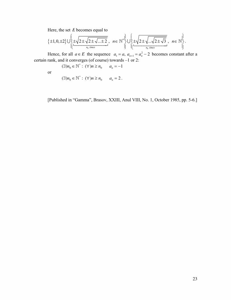
Here, the set E becomes equal to
{ }0 0
*
1,0, 2 2 2 ... 2 , 2 ... 2 3 , n times n times
n n⎧ ⎫⎧ ⎫⎪ ⎪ ⎪ ⎪± ± ± ± ± ± ∈ ± ± ± ∈⎨ ⎬ ⎨ ⎬
⎪ ⎪ ⎪ ⎪⎩ ⎭ ⎩ ⎭∪ ∪N N .
Hence, for all a ∈E the sequence a1 = a, an+1 = an2 − 2 becomes constant after a
certain rank, and it converges (of course) towards –1 or 2:
(∃)n0 ∈N* : (∀)n ≥ n0 an = −1 or (∃)n0 ∈N* : (∀)n ≥ n0 an = 2 . [Published in “Gamma”, Brasov, XXIII, Anul VIII, No. 1, October 1985, pp. 5-6.]
24
ON CARMICHAËL’S CONJECTURE
Carmichaël’s conjecture is the following: “the equation ϕ(x) = n cannot have a unique solution, (∀)n ∈N , where ϕ is the Euler’s function”. R. K. Guy presented in [1] some results on this conjecture; Carmichaël himself proved that, if n0 does not verify his conjecture, then n0 > 1037 ; V. L. Klee [2] improved to n0 > 10400 , and P. Masai & A. Valette increased to n0 > 1010000 . C. Pomerance [4] wrote on this subject too. In this article we prove that the equation ϕ(x) = n admits a finite number of solutions, we find the general form of these solutions, also we prove that, if x0 is the unique solution of this equation (for a n∈N ), then x0 is a multiple of 22 ⋅ 32 ⋅ 72 ⋅ 432 (and x0 > 1010000 from [3]). §1. Let x0 be a solution of the equation ϕ(x) = n . We consider n fixed. We’ll try to construct another solution y0 ≠ x0 . The first method: We decompose x0 = a ⋅ b with , a b integers such that (a, b) = 1.
we look for an a ' ≠ a such that ϕ(a ') = ϕ(a) and (a’, b) = 1; it results that y0 = a '⋅ b . The second method: Let’s consider x0 = q1
β1 ...qrβr , where all βi ∈N* , and q1,...,qr are distinct primes
two by two; we look for an integer q such that (q, x0) = 1 and ϕ(q) divides x0 / (q1,...,qr ) ; then y0 = x0q / ϕ(q) . We immediately see that we can consider q as prime. The author conjectures that for any integer x0 ≥ 2 it is possible to find, by means of one of these methods, a y0 ≠ x0 such that ϕ(y0 ) = ϕ(x0 ) . Lemma 1. The equation ϕ(x) = n admits a finite number of solutions, (∀)n ∈N . Proof. The cases n = 0,1 are trivial. Let’s consider n to be fixed, 2n ≥ . Let p1 < p2 < ... < ps ≤ n + 1 be the sequence of prime numbers. If x0 is a solution of our equation (1) then 0x has the form x0 = p1
α1 ...psα s , with all α i ∈N . Each α i is limited, because:
{ }( ) 1,2,..., , ( ) : ii ii s a p nα∀ ∈ ∃ ∈ ≥N .
Whence 0 ≤ α i ≤ ai + 1 , for all i . Thus, we find a wide limitation for the number of
solutions: (ai + 2)i=1
s
∏
Lemma 2. Any solution of this equation has the form (1) and (2):
25
10
1
1
....1 1
s
s
sppx np p
εε⎛ ⎞⎛ ⎞
= ⋅ ∈⎜ ⎟⎜ ⎟− −⎝ ⎠ ⎝ ⎠Z ,
where, for 1 i s≤ ≤ , we have 0iε = if 0iα = , or 1iε = if 0iα ≠ .
Of course, 10 0
1
1
( ) ....1 1
s
s
sppn x xp p
εε
ϕ⎛ ⎞⎛ ⎞
= = ⎜ ⎟⎜ ⎟− −⎝ ⎠ ⎝ ⎠,
whence it results the second form of x0 . From (2) we find another limitation for the number of the solutions: 2s − 1 because each ε i has only two values, and at least one is not equal to zero. §2. We suppose that x0 is the unique solution of this equation. Lemma 3. x0 is a multiple of 22 ⋅ 32 ⋅ 72 ⋅ 432 . Proof. We apply our second method. Because ϕ(0) = ϕ(3) and ϕ(1) = ϕ(2) we take x0 ≥ 4 . If 2 /| x0 then there is y0 = 2x0 ≠ x0 such that ϕ(y0 ) = ϕ(x0 ) , hence 2 | x0 ; if 4 /| x0 , then we can take y0 = x0 / 2 . If 3 /| x0 then y0 = 3x0 / 2 , hence 3 | x0 ; if 9 /| x0 then y0 = 2x0 / 3 , hence 9 | x0 ; whence 4 ⋅ 9 | x0 . If 7 /| x0 then 0 07 / 6y x= , hence 07 | x ; if 049 | x/ then 0 06 / 7y x= hence 049 | x ;
whence 04 9 49 | x⋅ ⋅ .
If 043 | x/ then 0 043 / 42y x= , hence 043 | x ; if 432 /| x0 then y0 = 42x0 / 43 , hence 432 | x0 ; whence 22 ⋅ 32 ⋅ 72 ⋅ 432 | x0 . Thus x0 = 2γ 1 ⋅ 3γ 2 ⋅ 7γ 3 ⋅ 43γ 4 ⋅ t , with all γ i ≥ 2 and (t, 2@3@7@43) = 1 and x0 > 1010000 because n0 > 1010000 . §3. Let’s consider m1 ≥ 3. If 5 /| x0 then 5x0 / 4 = y0 , hence 5 | x0 ; if 25 /| x0 then y0 = 4x0 / 5 , whence 25 | x0 . We construct the recurrent set M of prime numbers:
a) the elements 2, 3,5 ∈M ; b) if the distinct odd elements e1,...,en ∈M and bm = 1 + 2m ⋅ e1,...,en is prime,
with m = 1 or m = 2 , then bm ∈M ; c) any element belonging to M is obtained by the utilization (a finite number of
times) of the rules a) or b) only. The author conjectures that M is infinite, which solves this case, because it results
that there is an infinite number of primes which divide x0 . This is absurd. For example 2, 3, 5, 7, 11, 13, 23, 29, 31, 43, 47, 53, 61, … belong to M .
*
26
The method from §3 could be continued as a tree (for γ 2 ≥ 3 afterwards γ 3 ≥ 3 , etc.) but its ramifications are very complicated… REFERENCES
[1] R. K. Guy - Monthly unsolved problems - 1969-1983. Amer. Math. Monthly, Vol. 90, No. 10/1983, p. 684.
[2] V. L. Klee - Amer. Math. Monthly 76, (969), p. 288. [3] P. Masai & A. Valette - A lower bound for a counter-example to
Carmichaël’s conjecture - Boll. Unione Mat. Ital, (6) A1 (1982), pp. 313-316.
[4] C. Pomerance - Math. Reviews: 49:4917.
[Published in “Gamma”, XXIV, Year VIII, No. 2, February 1986, pp. 13-14.]
27
A PROPERTY FOR A COUNTEREXAMPLE TO CARMICHAËL’S CONJECTURE
Carmichaël has conjectured that: ( ) , ( ) n m∀ ∈ ∃ ∈N N , with m ≠ n , for which ϕ(n) = ϕ(m) , where ϕ is Euler’s totient function. There are many papers on this subject, but the author cites the papers which have influenced him, especially Klee’s papers. Let n be a counterexample to Carmichaël’s conjecture. Grosswald has proved that n is a multiple of 32, Donnelly has pushed the result to a multiple of 214 , and Klee to a multiple of 242 ⋅ 347 , Smarandache has shown that n is a multiple of 22 ⋅ 32 ⋅ 72 ⋅ 432 . Masai & Valette have bounded 1000010n > . In this note we will extend these results to: n is a multiple of a product of a very large number of primes. We construct a recurrent set M such that:
a) the elements 2,3 ∈M ; b) if the distinct elements 2, 3,q1,...,qr ∈M and 11 2 3a b
rp q q= + ⋅ ⋅ ⋅ ⋅ ⋅ is a prime, where { }0,1,2,..., 41a ∈ and { }0,1,2,..., 46b∈ , then p ∈M ; r ≥ 0 ;
c) any element belonging to M is obtained only by the utilization (a finite number of times) of the rules a) or b). Of course, all elements from M are primes. Let n be a multiple of 242 ⋅ 347 ;
if 5 /| n then there exists m = 5n/4 … n such that ϕ(n) = ϕ(m) ; hence 5 | n ; whence 5 ∈M ; if 52 /| n then there exists m = 4n/5 … n with our property; hence 52 | n ; analogously, if 7 /| n we can take 7 / 6m n n= ≠ , hence 7 | n ; if 72 /| n we can take m = 6n / 7 ≠ n ; whence 7 ∈M and 72 | n ; etc. The method continues until it isn’t possible to add any other prime to M , by its construction. For example, from the 168 primes smaller than 1000, only 17 of them do not belong to M (namely: 101, 151, 197, 251, 401, 491, 503, 601, 607, 677, 701, 727, 751, 809, 883, 907, 983); all other 151 primes belong to M . Note { }1 22,3, , ,..., ,...sM p p p= , then n is a multiple of 242 ⋅ 347 ⋅ p1
2 ⋅ p22 ⋅ ⋅ ⋅ ps
2 ⋅ ⋅ ⋅ From our example, it results that M contains at least 151 elements, hence s ≥ 149 . If M is infinite then there is no counterexample n , whence Carmichaël’s conjecture is solved. (The author conjectures M is infinite.) Using a computer it is possible to find a very large number of primes, which divide n , using the construction method of M , and trying to find a new prime p if p − 1 is a product of primes only from M .
28
REFERENCES
[1] R. D. Carmichaël - Note on Euler’s φ function - Bull. Amer. Math. Soc. 28(1922), pp. 109-110.
[2] H. Donnelly - On a problem concerning Euler’s phi-function - Amer. Math. Monthly, 80(1973), pp. 1029-1031.
[3] E. Grosswald - Contribution to the theory of Euler’s function φ(x) - Bull. Amer. Math. Soc., 79(1973), pp. 337-341.
[4] R. K. Guy - Monthly Research Problems - 1969-1973, Amer. Math. Monthly 80(1973), pp. 1120-1128.
[5] R. K. Guy - Monthly Research Problems - 1969-1983, Amer. Math. Monthly 90(1983), pp. 683-690.
[6] R. K. Guy - Unsolved Problems in Number Theory - Springer-Verlag, 1981, problem B 39, 53.
[7] V. L. Klee - On a conjecture of Carmichaël - Bull. Amer. Math. Soc 53 (1947), pp. 1183-1186.
[8] V. L. Klee - Is there a n for which φ(x) has a unique solution? - Amer. Math. Monthly. 76(1969), pp. 288-289.
[9] P. Masai et A. Valette - A lower bound for a counterexample to Carmichaël’s conjecture - Boll. Unione Mat. Ital. (6) A1(1982), pp. 313-316.
[10] F. Gh. Smarandache - On Carmichaël’s conjecture - Gamma, Braşov, XXIV, Year VIII, 1986.
[Published in “Gamma”, XXV, Year VIII, No. 3, June 1986, pp. 4-5.]
29
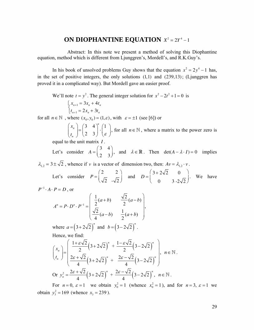
ON DIOPHANTINE EQUATION X 2 = 2Y 4 − 1
Abstract: In this note we present a method of solving this Diophantine equation, method which is different from Ljunggren’s, Mordell’s, and R.K.Guy’s. In his book of unsolved problems Guy shows that the equation x2 = 2y4 − 1 has, in the set of positive integers, the only solutions (1,1) and (239,13) ; (Ljunggren has proved it in a complicated way). But Mordell gave an easier proof. We’ll note t = y2 . The general integer solution for 2 22 1 0x t− + = is
xn+1 = 3xn + 4tn
tn+1 = 2xn + 3tn
⎧⎨⎩
for all n ∈N , where (x0 , y0 ) = (1,ε ) , with ε = ±1 (see [6]) or
3 4 1 2 3
nn
n
x
t ε⎛ ⎞ ⎛ ⎞ ⎛ ⎞
= ⋅⎜ ⎟ ⎜ ⎟ ⎜ ⎟⎜ ⎟ ⎝ ⎠ ⎝ ⎠⎝ ⎠, for all n ∈N , where a matrix to the power zero is
equal to the unit matrix I .
Let’s consider A =3 4
2 3
⎛⎝⎜
⎞⎠⎟
, and λ ∈R . Then det(A − λ ⋅ I ) = 0 implies
λ1,2 = 3 ± 2 , whence if v is a vector of dimension two, then: Av = λ1,2 ⋅ v .
Let’s consider P =2 2
2 - 2
⎛
⎝⎜⎞
⎠⎟ and D =
3 + 2 2 0
0 3 -2 2
⎛
⎝⎜
⎞
⎠⎟ . We have
P−1 ⋅ A ⋅ P = D , or
1
1 2 ( ) ( )2 22 1( ) ( )
4 2
n na b a b
A P D Pa b a b
−
⎛ ⎞+ −⎜ ⎟
⎜ ⎟= ⋅ ⋅ =⎜ ⎟
− +⎜ ⎟⎝ ⎠
,
where ( )3 2 2n
a = + and ( )3 2 2n
b = − .
Hence, we find:
( ) ( )
( ) ( )
1 2 1 2 3 2 2 + 3 2 22 2
2 2 2 23 2 2 + 3 2 24 4
n n
n
n nn
x
t
ε ε
ε ε
⎛ ⎞+ −+ −⎜ ⎟⎛ ⎞
⎜ ⎟=⎜ ⎟⎜ ⎟ ⎜ ⎟+ −⎝ ⎠ + −⎜ ⎟⎝ ⎠
, n ∈N .
Or ( ) ( )2 2 2 2 23 2 2 + 3 2 24 4
n n
ny ε ε+ −= + − , n ∈N .
For 0, 1n ε= = we obtain y02 = 1 (whence x0
2 = 1 ), and for 3, 1n ε= = we
obtain 23 169y = (whence 3 239x = ).
30
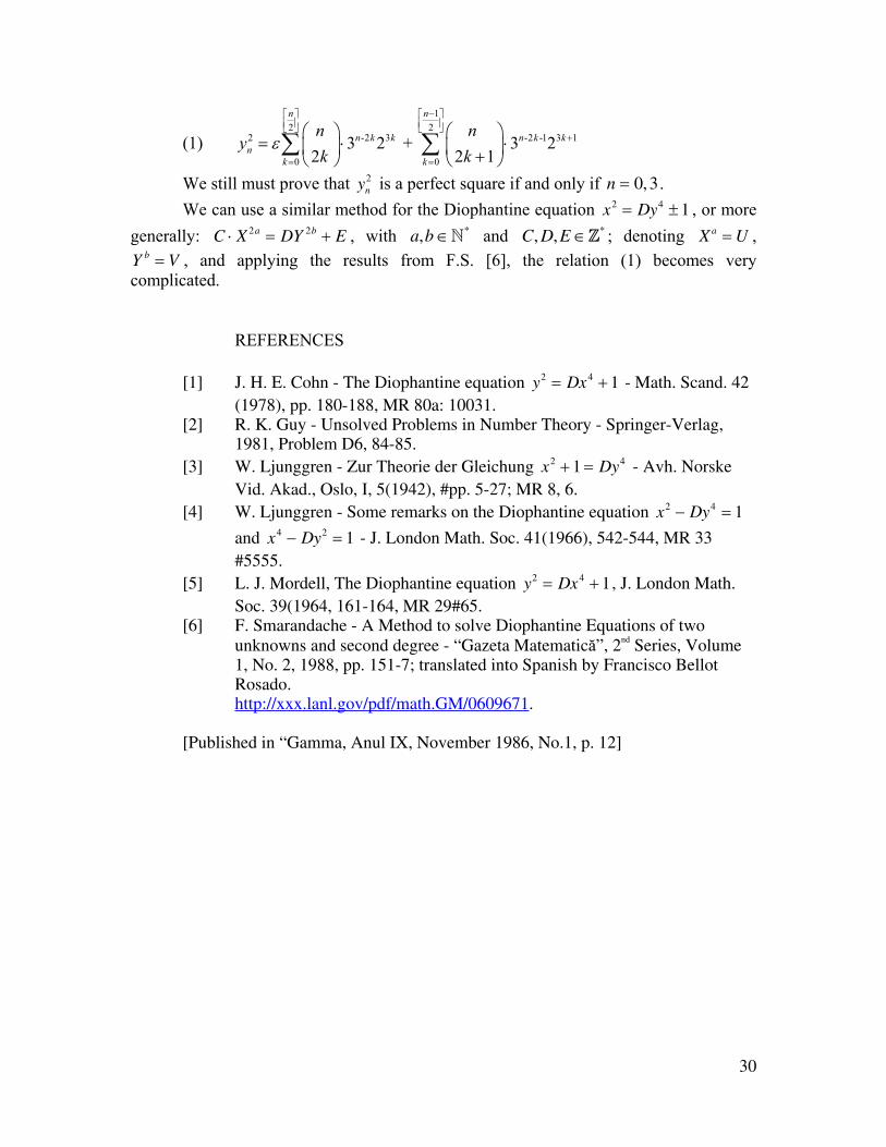
(1)
12 2
2 -2 3 -2 -1 3 1
0 0
3 2 + 3 2
2 2 1
n n
n k k n k kn
k k
n ny
k kε
−⎡ ⎤ ⎡ ⎤⎢ ⎥ ⎢ ⎥⎣ ⎦ ⎣ ⎦
+
= =
⎛ ⎞ ⎛ ⎞= ⋅ ⋅⎜ ⎟ ⎜ ⎟+⎝ ⎠ ⎝ ⎠
∑ ∑
We still must prove that yn2 is a perfect square if and only if n = 0,3 .
We can use a similar method for the Diophantine equation x2 = Dy4 ± 1 , or more generally: C ⋅ X 2a = DY 2b + E , with a,b ∈N* and C, D,E ∈Z* ; denoting X a = U , Y b = V , and applying the results from F.S. [6], the relation (1) becomes very complicated.
REFERENCES
[1] J. H. E. Cohn - The Diophantine equation y2 = Dx4 + 1 - Math. Scand. 42 (1978), pp. 180-188, MR 80a: 10031.
[2] R. K. Guy - Unsolved Problems in Number Theory - Springer-Verlag, 1981, Problem D6, 84-85.
[3] W. Ljunggren - Zur Theorie der Gleichung x2 + 1 = Dy4 - Avh. Norske Vid. Akad., Oslo, I, 5(1942), #pp. 5-27; MR 8, 6.
[4] W. Ljunggren - Some remarks on the Diophantine equation x2 − Dy4 = 1
and x4 − Dy2 = 1 - J. London Math. Soc. 41(1966), 542-544, MR 33 #5555.
[5] L. J. Mordell, The Diophantine equation y2 = Dx4 + 1, J. London Math. Soc. 39(1964, 161-164, MR 29#65.
[6] F. Smarandache - A Method to solve Diophantine Equations of two unknowns and second degree - “Gazeta Matematică”, 2nd Series, Volume 1, No. 2, 1988, pp. 151-7; translated into Spanish by Francisco Bellot Rosado.
http://xxx.lanl.gov/pdf/math.GM/0609671.
[Published in “Gamma, Anul IX, November 1986, No.1, p. 12]
31
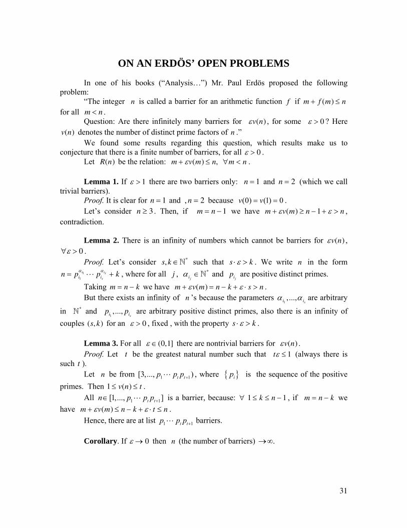
ON AN ERDÖS’ OPEN PROBLEMS In one of his books (“Analysis…”) Mr. Paul Erdös proposed the following problem: “The integer n is called a barrier for an arithmetic function f if m + f (m) ≤ n for all m < n .
Question: Are there infinitely many barriers for εv(n) , for some ε > 0 ? Here v(n) denotes the number of distinct prime factors of n .” We found some results regarding this question, which results make us to conjecture that there is a finite number of barriers, for all ε > 0 . Let R(n) be the relation: m + εv(m) ≤ n, ∀m < n . Lemma 1. If ε > 1 there are two barriers only: n = 1 and n = 2 (which we call trivial barriers). Proof. It is clear for n = 1 and , n = 2 because (0) (1) 0v v= = . Let’s consider n ≥ 3 . Then, if m = n − 1 we have m + εv(m) ≥ n − 1 + ε > n , contradiction. Lemma 2. There is an infinity of numbers which cannot be barriers for εv(n) , ∀ε > 0 . Proof. Let’s consider s,k ∈N* such that s ⋅ ε > k . We write n in the form n = pi1
α i1 ⋅ ⋅ ⋅ pis
α is + k , where for all j , α i j∈N* and pij
are positive distinct primes. Taking m = n − k we have m + εv(m) = n − k + ε ⋅ s > n . But there exists an infinity of n ’s because the parameters α i1
,...,α isare arbitrary
in N* and pi1
,..., pis are arbitrary positive distinct primes, also there is an infinity of
couples (s, k) for an ε > 0 , fixed , with the property s ⋅ ε > k . Lemma 3. For all ε ∈(0,1] there are nontrivial barriers for εv(n) . Proof. Let t be the greatest natural number such that tε ≤ 1 (always there is such t ). Let n be from 1 1[3,..., )t tp p p +⋅ ⋅⋅ , where { }ip is the sequence of the positive primes. Then 1 ≤ v(n) ≤ t . All 1 1[1,..., ]t tn p p p +∈ ⋅⋅⋅ is a barrier, because: ∀ 1 ≤ k ≤ n − 1 , if m = n − k we have m + εv(m) ≤ n − k + ε ⋅ t ≤ n . Hence, there are at list 1 1t tp p p +⋅⋅⋅ barriers. Corollary. If ε → 0 then n (the number of barriers) →∞.
32
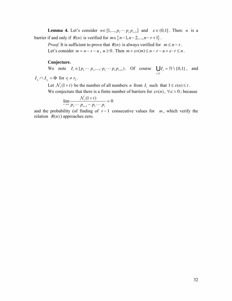
Lemma 4. Let’s consider 1 1[1,..., ]r rn p p p +∈ ⋅⋅⋅ and ε ∈(0,1] . Then: n is a barrier if and only if R(n) is verified for { }1, 2,..., 1m n n n r∈ − − − + . Proof. It is sufficient to prove that R(n) is always verified for m ≤ n − r . Let’s consider m = n − r − u , u ≥ 0 . Then m + εv(m) ≤ n − r − u + ε ⋅ r ≤ n . Conjecture. We note Ir ∈[ p1 ⋅ ⋅ ⋅ pr ,...,⋅p1 ⋅ ⋅ ⋅ pr pr +1) . Of course
Ir
r ≥1U = N \ {0,1} , and
Ir1∩ Ir2
= Φ for r1 ≠ r2 . Let Nr (1+ t) be the number of all numbers n from Ir such that 1 ≤ v(n) ≤ t .
We conjecture that there is a finite number of barriers for εv(n) , ∀ε > 0 ; because
limr→∞
N r (1+ t)
p1 ⋅ ⋅ ⋅ pr +1 − p1 ⋅ ⋅ ⋅ pr
= 0
and the probability (of finding of r − 1 consecutive values for m , which verify the relation R(n) ) approaches zero.
33
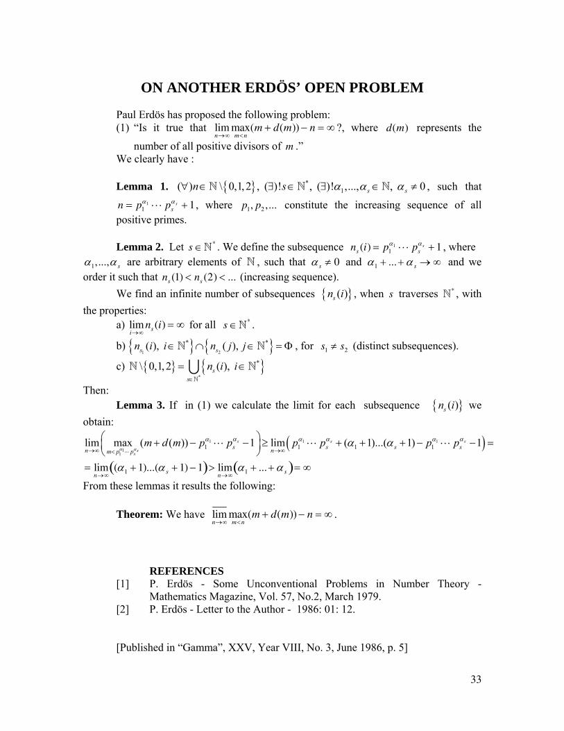
ON ANOTHER ERDÖS’ OPEN PROBLEM Paul Erdös has proposed the following problem:
(1) “Is it true that limn→∞
maxm<n
(m + d(m)) − n = ∞ ?, where d(m) represents the
number of all positive divisors of m .” We clearly have : Lemma 1. { } *
1( ) \ 0,1,2 , ( )! , ( )! ,..., , 0s sn s α α α∀ ∈ ∃ ∈ ∃ ∈ ≠N N N , such that
n = p1α1 ⋅ ⋅ ⋅ ps
α s + 1 , where p1, p2 ,... constitute the increasing sequence of all positive primes. Lemma 2. Let s ∈N* . We define the subsequence ns (i) = p1
α1 ⋅ ⋅ ⋅ psα s + 1 , where
α1,...,α s are arbitrary elements of N , such that α s ≠ 0 and α1 + ... + α s → ∞ and we order it such that ns (1) < ns (2) < ... (increasing sequence).
We find an infinite number of subsequences { }( )sn i , when s traverses N* , with
the properties: a) lim
i→∞ns (i) = ∞ for all s ∈N* .
b) { } { }1 2
* *( ), ( ), s sn i i n j j∈ ∩ ∈ = ΦN N , for s1 ≠ s2 (distinct subsequences).
c) { } { }*
*\ 0,1,2 ( ), ss
n i i∈
= ∈∪N
N N
Then: Lemma 3. If in (1) we calculate the limit for each subsequence { }( )sn i we obtain:
( )1 1 1
11
1 1 1 1lim max ( ( )) 1 lim ( 1)...( 1) 1s s s
ss
s s s sn nm p pm d m p p p p p p
α α
α α αα α αα α→∞ →∞< ⋅⋅⋅
⎛ ⎞+ − ⋅⋅⋅ − ≥ ⋅⋅⋅ + + + − ⋅⋅⋅ − =⎜ ⎟⎝ ⎠
= limn→∞
(α1 + 1)...(α s + 1) − 1( )> limn→∞
α1 + ... + α s( )= ∞
From these lemmas it results the following: Theorem: We have lim
n→∞maxm<n
(m + d(m)) − n = ∞ .
REFERENCES
[1] P. Erdös - Some Unconventional Problems in Number Theory - Mathematics Magazine, Vol. 57, No.2, March 1979.
[2] P. Erdös - Letter to the Author - 1986: 01: 12. [Published in “Gamma”, XXV, Year VIII, No. 3, June 1986, p. 5]
34
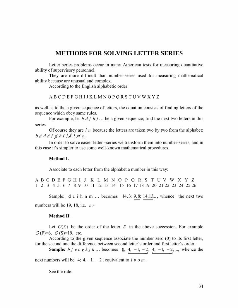
METHODS FOR SOLVING LETTER SERIES
Letter series problems occur in many American tests for measuring quantitative ability of supervisory personnel. They are more difficult than number-series used for measuring mathematical ability because are unusual and complex. According to the English alphabetic order: A B C D E F G H I J K L M N O P Q R S T U V W X Y Z as well as to the a given sequence of letters, the equation consists of finding letters of the sequence which obey same rules. For example, let b d f h j … be a given sequence; find the next two letters in this series. Of course they are l n because the letters are taken two by two from the alphabet: b c d e f g h i j k l m n . In order to solve easier letter –series we transform them into number-series, and in this case it’s simpler to use some well-known mathematical procedures. Method I. Associate to each letter from the alphabet a number in this way: A B C D E F G H I J K L M N O P Q R S T U V W X Y Z 1 2 3 4 5 6 7 8 9 10 11 12 13 14 15 16 17 18 19 20 21 22 23 24 25 26 Sample: d c i h n m … becomes 14,3; 9,8; 14,13... , whence the next two
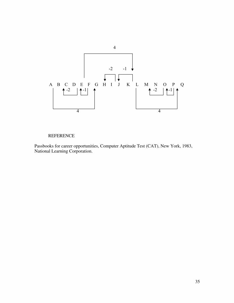
numbers will be 19, 18, i.e. s r Method II. Let O(L) be the order of the letter L in the above succession. For example O (F)=6, O (S)=19, etc. According to the given sequence associate the number zero (0) to its first letter, for the second one the difference between second letter’s order and first letter’s order, Sample: b f e c g k j h … becomes 0, 4, 1, 2; 4, 1, 2;...,− − − − whence the
next numbers will be 4; 4, − 1, − 2 ; equivalent to l p o m . See the rule:
35
REFERENCE Passbooks for career opportunities, Computer Aptitude Test (CAT), New York, 1983, National Learning Corporation.
4
-2 -1
A B C D E F G H I J K L M N O P Q -2 -1 -2 -1 4 4
36
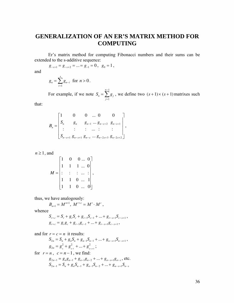
GENERALIZATION OF AN ER’S MATRIX METHOD FOR COMPUTING
Er’s matrix method for computing Fibonacci numbers and their sums can be extended to the s-additive sequence:
g− s+1 = g− s+ 2 = ... = g−1 = 0 , g0 = 1 , and
gn = gn− ii=1
s
∑ for n > 0 .
For example, if we note Sn = gjj =1
n−1
∑ , we define two (s + 1) × (s + 1) matrixes such
that:
Bn =
1 0 0 ... 0 0
Sn gn gn−1 ... gn− s+2 gn− s+1
: : : ... : :
Sn− s+1 gn− s+1 gn− s ... gn− 2s+ 3 gn−2s+2
⎡
⎣
⎢⎢⎢⎢
⎤
⎦
⎥⎥⎥⎥
,
n ≥ 1, and
M =
1 0 0 ... 0
1 1 1 ... 0
: : : ... :
1 1 0 ... 1
1 1 0 ... 0
⎡
⎣
⎢⎢⎢⎢⎢⎢
⎤
⎦
⎥⎥⎥⎥⎥⎥
,
thus, we have analogously: 1
1 , n r c r cnB M M M M+ +
+ = = ⋅ , whence Sr +c = Sr + grSc + gr −1Sc−1 + ... + gr − s+1Sc− s+1 , gr +c = grgc + gr −1gc−1 + ... + gr − s+1gc− s+1 , and for r = c = n it results: S2n = Sn + gnSn + gn−1Sn−1 + ... + gn− s+1Sn− s+1 , g2n = g
n
2 + gn−1
2 + ...+ gn−s+1
2 ; for r = n , c = n − 1 , we find: g2n−1 = gngn−1 + gn−1gn− 2 + ... + gn− s+1gn− s , etc. S2n−1 = Sn + gnSn−1 + gn−1Sn−2 + ... + gn− s+1Sn− s
37
Whence we can construct a similar algorithm as M. C. Er for computing s-additive numbers and their sums. REFERENCE:
M. C. Er, Fast Computation of Fibonacci Numbers and Their Sums, J. Inf. Optimization Sci. (Delhi), Vol. 6 (1985), No. 1. pp. 41-47. [Published in “GAMMA”, Braşov, Anul X, No.. 1-2, October 1987, p. 8]
38
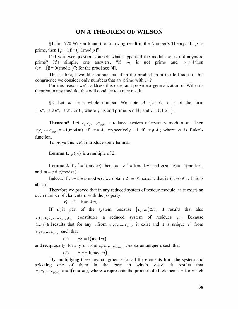
ON A THEOREM OF WILSON
§1. In 1770 Wilson found the following result in the Number’s Theory: “If p is prime, then p − 1( )! ≡ −1mod p( )”.
Did you ever question yourself what happens if the module m is not anymore prime? It’s simple, one answers, “if m is not prime and m ≠ 4 then
m − 1( )! ≡ 0 mod m( )”; for the proof see [4]. This is fine, I would continue, but if in the product from the left side of this
congruence we consider only numbers that are prime with m ? For this reason we’ll address this case, and provide a generalization of Wilson’s
theorem to any modulo, this will conduce to a nice result. §2. Let m be a whole number. We note { , A x= ∈Z x is of the form
± pn , ± 2 pn , ± 2r , or 0 , where p is odd prime, n ∈N , and r = 0,1,2 } . Theorem*. Let c1,c2 ,...,cϕ (m ) a reduced system of residues modulo m . Then
c1c2 . ⋅ ⋅ ⋅ cϕ (m ) ≡ −1(mod m) if m ∈A , respectively +1 if m ∉A ; where ϕ is Euler’s function.
To prove this we’ll introduce some lemmas. Lemma 1. ϕ(m) is a multiple of 2. Lemma 2. If c2 ≡ 1(mod m) then (m − c)2 ≡ 1(mod m) and c(m − c) ≡ −1(mod m) ,
and m − c /≡ c(mod m) . Indeed, if m − c ≡ c(mod m) , we obtain 2c ≡ 0(mod m) , that is (c, m) /≡ 1 . This is
absurd. Therefore we proved that in any reduced system of residue modulo m it exists an
even number of elements c with the property P1 : c2 ≡ 1(mod m) .
If ci0is part of the system, because ( )0
, 1ic m ≅ , it results that also
c1ci0,c2ci0
,...,cϕ (m )ci0 constitutes a reduced system of residues m . Because
(1,m) ≅ 1 results that for any c from c1,c2 ,...,cϕ (m ) it exist and it is unique c ' from c1,c2 ,...,cϕ (m ) such that (1) cc ' ≡ 1 mod m( ) and reciprocally: for any c ' from c1,c2 ,...,cϕ (m ) it exists an unique c such that (2) c 'c ≡ 1 mod m( ).
By multiplying these two congruence for all the elements from the system and selecting one of them in the case in which c ≠ c ' it results that c1,c2 ,...,cϕ (m ) ⋅b ≡ 1 mod m( ), where b represents the product of all elements c for which
39
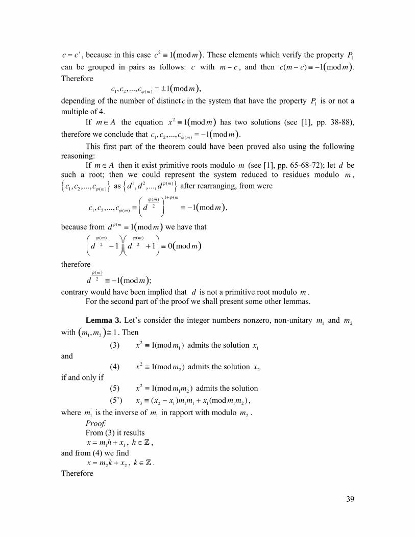
c = c ' , because in this case c2 ≡ 1 mod m( ). These elements which verify the property P1 can be grouped in pairs as follows: c with m − c , and then c(m − c) ≡ −1 mod m( ). Therefore
c1,c2 ,...,cϕ (m ) ≡ ±1 mod m( ), depending of the number of distinct c in the system that have the property P1 is or not a multiple of 4. If m ∈A the equation x2 ≡ 1 mod m( ) has two solutions (see [1], pp. 38-88), therefore we conclude that c1,c2 ,...,cϕ (m ) ≡ −1 mod m( ). This first part of the theorem could have been proved also using the following reasoning:
If m ∈A then it exist primitive roots modulo m (see [1], pp. 65-68-72); let d be such a root; then we could represent the system reduced to residues modulo m , { }1 2 ( ), ,..., mc c cϕ as { }1 2 ( ), ,..., md d dϕ after rearranging, from were
c1,c2 ,...,cϕ (m ) ≡ dϕ (m )
2⎛⎝⎜
⎞⎠⎟
1+ϕ (m
≡ −1 mod m( ),
because from dϕ (m ≡ 1 mod m( ) we have that
dϕ (m)
2 − 1⎛⎝⎜
⎞⎠⎟
dϕ (m)
2 + 1⎛⎝⎜
⎞⎠⎟
≡ 0 mod m( )
therefore
dϕ (m )
2 ≡ −1 mod m( ); contrary would have been implied that d is not a primitive root modulo m . For the second part of the proof we shall present some other lemmas. Lemma 3. Let’s consider the integer numbers nonzero, non-unitary m1 and m2 with m1, m2( )≅ 1 . Then (3) x2 ≡ 1(mod m1) admits the solution x1 and (4) x2 ≡ 1(mod m2 ) admits the solution x2 if and only if (5) x2 ≡ 1(mod m1m2 ) admits the solution (5’) x3 ≡ (x2 − x1)m1
' m1 + x1(mod m1m2 ) , where m1
' is the inverse of m1 in rapport with modulo m2 . Proof. From (3) it results
x = m1h + x1 , h ∈Z , and from (4) we find
x = m2k + x2 , k ∈Z . Therefore
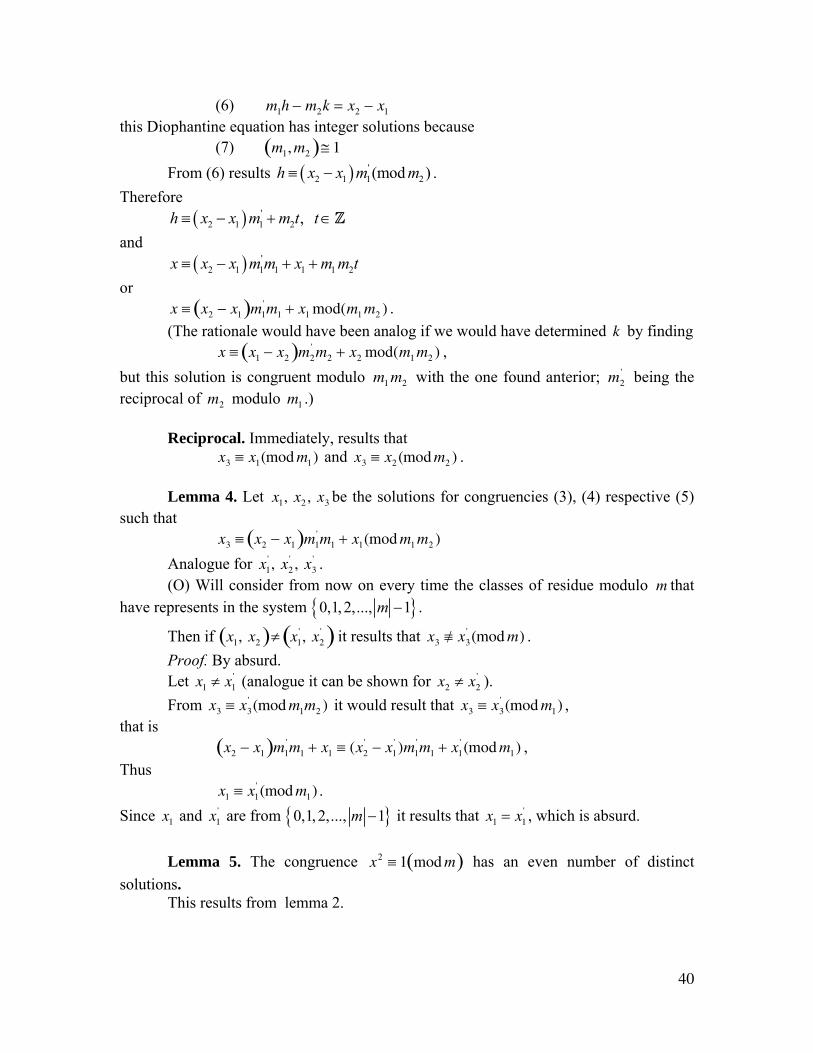
40
(6) m1h − m2k = x2 − x1 this Diophantine equation has integer solutions because (7) m1, m2( )≅ 1 From (6) results ( ) '
2 1 1 2(mod )h x x m m≡ − . Therefore
( ) '2 1 1 2 , h x x m m t t≡ − + ∈Z
and ( ) '
2 1 1 1 1 1 2x x x m m x m m t≡ − + + or
x ≡ x2 − x1( )m1' m1 + x1 mod(m1 m2 ) .
(The rationale would have been analog if we would have determined k by finding x ≡ x1 − x2( )m2
' m2 + x2 mod(m1 m2 ) , but this solution is congruent modulo m1 m2 with the one found anterior; m2
' being the reciprocal of m2 modulo m1 .) Reciprocal. Immediately, results that
x3 ≡ x1(mod m1) and x3 ≡ x2 (mod m2 ) .
Lemma 4. Let x1, x2 , x3 be the solutions for congruencies (3), (4) respective (5) such that
x3 ≡ x2 − x1( )m1' m1 + x1(mod m1 m2 )
Analogue for x1' , x2
' , x3' .
(O) Will consider from now on every time the classes of residue modulo m that have represents in the system { }0,1, 2,..., 1m − .
Then if x1, x2( )≠ x1' , x2
'( ) it results that x3 /≡ x3' (mod m) .
Proof. By absurd. Let x1 ≠ x1
' (analogue it can be shown for x2 ≠ x2' ).
From x3 ≡ x3' (mod m1m2 ) it would result that x3 ≡ x3
' (mod m1) , that is
x2 − x1( )m1' m1 + x1 ≡ (x2
' − x1' )m1
' m1 + x1' (mod m1) ,
Thus x1 ≡ x1
' (mod m1) . Since x1 and x1
' are from { }0,1, 2,..., 1m − it results that x1 = x1' , which is absurd.
Lemma 5. The congruence x2 ≡ 1 mod m( ) has an even number of distinct
solutions. This results from lemma 2.
41
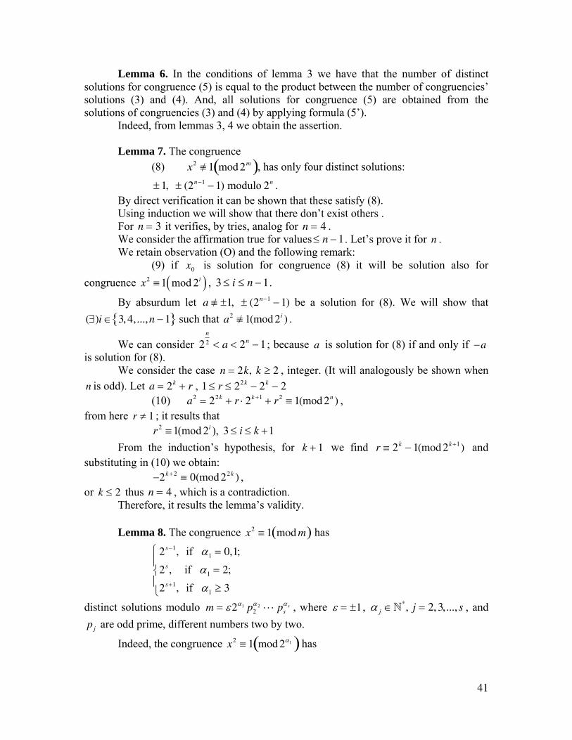
Lemma 6. In the conditions of lemma 3 we have that the number of distinct solutions for congruence (5) is equal to the product between the number of congruencies’ solutions (3) and (4). And, all solutions for congruence (5) are obtained from the solutions of congruencies (3) and (4) by applying formula (5’).
Indeed, from lemmas 3, 4 we obtain the assertion. Lemma 7. The congruence (8) x2 /≡ 1 mod 2m( ), has only four distinct solutions:
± 1, ± (2n−1 − 1) modulo 2n . By direct verification it can be shown that these satisfy (8). Using induction we will show that there don’t exist others . For n = 3 it verifies, by tries, analog for n = 4 . We consider the affirmation true for values ≤ n − 1 . Let’s prove it for n . We retain observation (O) and the following remark: (9) if x0 is solution for congruence (8) it will be solution also for
congruence ( )2 1 mod 2ix ≡ , 3 ≤ i ≤ n − 1.
By absurdum let a /≡ ±1, ± (2n−1 − 1) be a solution for (8). We will show that (∃)i ∈ 3, 4,...,n − 1{ } such that a2 /≡ 1(mod 2i ) .
We can consider 2n
2 < a < 2n − 1 ; because a is solution for (8) if and only if −a is solution for (8).
We consider the case n = 2k, k ≥ 2 , integer. (It will analogously be shown when n is odd). Let a = 2k + r , 1 ≤ r ≤ 22k − 2k − 2
(10) a2 = 22k + r ⋅ 2k +1 + r2 ≡ 1(mod 2n ) , from here r ≠ 1 ; it results that
2 1(mod 2 ), 3 1ir i k≡ ≤ ≤ + From the induction’s hypothesis, for k + 1 we find r ≡ 2k − 1(mod 2k +1) and substituting in (10) we obtain:
−2k +2 ≡ 0(mod 22k ) , or k ≤ 2 thus n = 4 , which is a contradiction.
Therefore, it results the lemma’s validity. Lemma 8. The congruence x2 ≡ 1 mod m( ) has
2s−1, if α1 = 0,1;
2s , if α1 = 2;
2s+1, if α1 ≥ 3
⎧
⎨⎪
⎩⎪
distinct solutions modulo m = ε2α1 p2α2 ⋅ ⋅ ⋅ ps
α s , where ε = ±1 , α j ∈N*, j = 2,3,..., s , and pj are odd prime, different numbers two by two.
Indeed, the congruence x2 ≡ 1 mod 2α1( ) has
42
1, if α1 = 0,1;
2, if α1 = 2;
4, if α1 ≥ 3
⎧
⎨⎪
⎩⎪
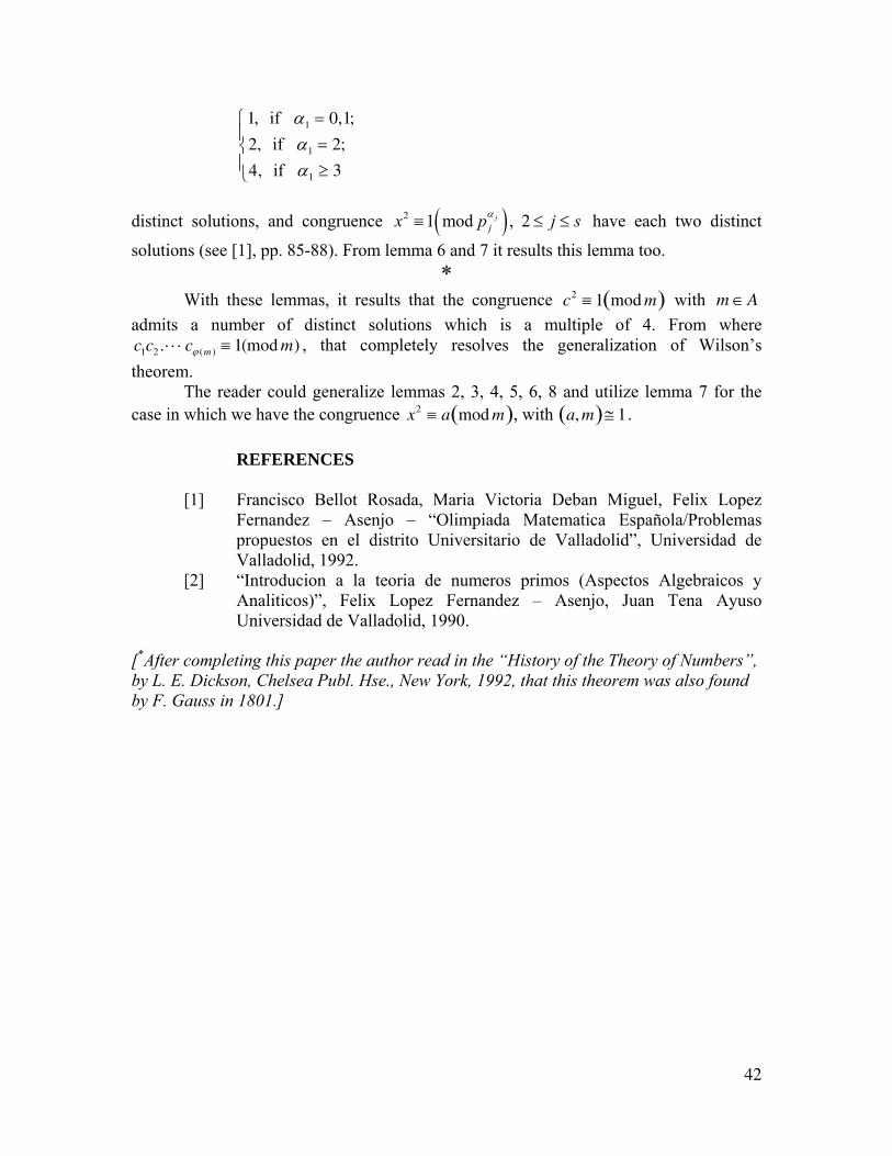
distinct solutions, and congruence ( )2 1 mod , 2j
jx p j sα≡ ≤ ≤ have each two distinct
solutions (see [1], pp. 85-88). From lemma 6 and 7 it results this lemma too. *
With these lemmas, it results that the congruence c2 ≡ 1 mod m( ) with m ∈A admits a number of distinct solutions which is a multiple of 4. From where c1c2 . ⋅ ⋅ ⋅ cϕ (m ) ≡ 1(mod m) , that completely resolves the generalization of Wilson’s theorem. The reader could generalize lemmas 2, 3, 4, 5, 6, 8 and utilize lemma 7 for the case in which we have the congruence x2 ≡ a mod m( ), with a, m( )≅ 1 . REFERENCES
[1] Francisco Bellot Rosada, Maria Victoria Deban Miguel, Felix Lopez Fernandez – Asenjo – “Olimpiada Matematica Española/Problemas propuestos en el distrito Universitario de Valladolid”, Universidad de Valladolid, 1992.
[2] “Introducion a la teoria de numeros primos (Aspectos Algebraicos y Analiticos)”, Felix Lopez Fernandez – Asenjo, Juan Tena Ayuso Universidad de Valladolid, 1990.
[*After completing this paper the author read in the “History of the Theory of Numbers”, by L. E. Dickson, Chelsea Publ. Hse., New York, 1992, that this theorem was also found by F. Gauss in 1801.]
43
A METHOD OF RESOLVING IN INTEGER NUMBERS OF
CERTAIN NONLINEAR EQUATIONS
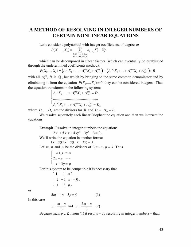
Let’s consider a polynomial with integer coefficients, of degree m P(X1,..., Xn ) = ai1 ...in
0≤i1 +...+ in ≤m0≤i j ≤m, j =1,n
∑ X1i1 ...Xn
in
which can be decomposed in linear factors (which can eventually be established through the undetermined coefficients method): P(X1,..., Xn ) = A1
(1)X1 + ... + An(1)Xn + An+1
(1)( )⋅ ⋅ ⋅ A1(m )X1 + ... + An
(m )Xn + An+1(m )( )+ B
with all Aj(k ), B in Q , but which by bringing to the same common denominator and by
eliminating it from the equation P(X1,..., Xn ) = 0 they can be considered integers.. Thus the equation transforms in the following system:
A1(1)X1 + ... + An
(1)Xn + An+1(1) = D1
................................................
A1(m )X1 + ... + An
(m )Xn + An+1(m ) = Dm
⎧
⎨⎪
⎩⎪
where D1,..., Dm are the divisors for B and D1 ⋅ ⋅ ⋅ Dm = B . We resolve separately each linear Diophantine equation and then we intersect the equations. Example. Resolve in integer numbers the equation: −2x3 + 5x2y + 4xy2 − 3y3 − 3 = 0 . We’ll write the equation in another format (x + y)(2x − y)(−x + 3y) = 3 . Let m, n and p be the divisors of 3, m ⋅ n ⋅ p = 3 . Thus
x + y = m
2x − y = n
−x + 3y = p
⎧
⎨⎪
⎩⎪
For this system to be compatible it is necessary that
1 1 m
2 − 1 n
−1 3 p
⎛
⎝
⎜⎜
⎞
⎠
⎟⎟
= 0 ,
or 5m − 4n − 3p = 0 (1) In this case
x =m + n
3 and y =
2m − n
3 (2)
Because m,n, p ∈Z , from (1) it results – by resolving in integer numbers – that:
44
m = 3k1 − k2
n = k2
p = 5k1 − 3k2
⎧
⎨⎪
⎩⎪
k1, k2 ∈Z
which substituted in (2) will give us x = k1 and y = 2k1 − k2 . But k2 ∈D(3) = ±1, ±3{ }; thus the only solution is obtained for k2 = 1 , k1 = 0 from where x = 0 and y = −1 . Analogue it can be shown that, for example the equation: −2x3 + 5x2y + 4xy2 − 3y3 = 6 does not have solutions in integer numbers. REFERENCES
[1] Marius Giurgiu, Cornel Moroti, Florică Puican, Stefan Smărăndoiu – Teme şi teste de Matematică pentru clasele IV-VIII - Ed. Matex, Rm. Vîlcea, Nr. 3/1991
[2] Ion Nanu, Lucian Tuţescu – “Ecuaţii Nestandard”, Ed. Apollo şi Ed. Oltenia, Craiova, 1994.
45
A GENERALIZATION REGARDING THE EXTREMES OF A TRIGONOMETRIQUE FUNCTION
After a passionate lecture of this book [1] (Mathematics plus literature!) I stopped at one of the problems explained here:
At page 121, the problem 2 asks to determine the maximum of expression: E(x) = (9 + cos2 x)(6 + sin2 x) . Analogue, in G. M. 7/1981, page 280, problem 18820*.
Here, we’ll present a generalization of these problems, and we’ll give a simpler solving method, as follows: Let 2 2
1 1 2 2: , ( ) ( sin )( cos )f f x a x b a x b→ = + + ; find the function’s extreme values. To solve it, we’ll take into account that we have the following relation: cos2 x = 1 − sin2 x , and we’ll note sin2 x = y . Thus y ∈[0,1] . The function becomes:
f (y) − (a1y + b1)(−a2y + a2 + b2 ) = −a1a2y2 + (a1a2 + a1b2 − a2b1)y + b1a2 + b1b2 , where y ∈[0,1] . Therefore f is a parabola. If a1a2 = 0 , the problem becomes banal.
If a1a2 > 0 , f (ymax ) =−Δ4a
, ymax =−b
2a (*)
a) when −b
2a∈[0,1] , the values that we are looking for are those from
(*), and
ymin = max −b
2a− 0,1 +
b
2a⎧⎨⎩
⎫⎬⎭
b) when −b
2a> 1 , we have ymax = 1 , ymin = 0 . (it is evident that
fmax = f (ymax ) and fmin = f (ymin ) )
c) when −b
2a< 0 , we have ymax = 0 , ymin = 1 .
If a1a2 < 0 , the function admits a minimum for
ymin = −b
2a, fmin
−Δ4a
(on the real axes) (**)
a) when −b
2a∈[0,1] , the looked after solutions are those from (**). And
ymax = max −b
2a,1 +
b
2a⎧⎨⎩
⎫⎬⎭
46
b) when −b
2a> 1 , we have ymax = 0 , ymin = 1
c) when −b
2a< 0 , we have ymax = 1 , ymin = 0 .
Maybe the cases presented look complicated and unjustifiable, but if you plot the parabola (or the line), then the reasoning is evident.
REFERENCE [1] Viorel Gh. Vod - Surprize în matematica elementar - Editura Albatros,
Bucure ti, 1981.
47
ON SOLVING HOMOGENE SYSTEMS
In the High School Algebra manual for grade IX (1981), pp. 103-104, is presented a method for solving systems of two homogenous equations of second degree, with two unknowns. In this article we’ll present another method of solving them. Let’s have the homogenous system
a1x
2 + b1xy + c1y2 = d1
a2 x2 + b2xy + c2y2 = d2
⎧⎨⎪
⎩⎪
with real coefficients. We will note x = ty , (or y = tx ), and by substitution, the system becomes:
2 2
1 1 1 12 2
2 2 2 2
( ) (1)
( ) (2)
y a t b t c d
y a t b t c d
⎧ + + =⎪⎨
+ + =⎪⎩
Dividing (1) by (2) and grouping the terms, it results an equation of second degree of variable t :
a1d2 − a2d1( )t 2 + b1d2 − b2d1( )t + c1d2 − c2d1( )= 0 If Δ t < 0 , the system doesn’t have solutions. If Δ t ≥ 0 , the initial system becomes equivalent with the following systems:
(S1)x = t1y
a1x2 + b1xy + c1y
2 = d1
⎧⎨⎩
and
(S2 )x = t2y
a1x2 + b1xy + c1y
2 = d1
⎧⎨⎩
which can simply be resolved by substituting the value of x from the first equation into the second. Further we will provide an extension of this method. Let have the homogeneous system:
,0
, 1,n
n i ii j
ia x y j m−
=
=∑
To resolve this, we note x = ty , it results:
yn ai, jtn− i = bj
i=0
n
∑ , j = 1,m
By dividing in order the first equation to the rest of them, we obtain:
,1 , 10 0
/ , 2,n n
n i n ii i j j
i ia t a t b b j m− −
= =
⎛ ⎞ ⎛ ⎞= =⎜ ⎟ ⎜ ⎟
⎝ ⎠ ⎝ ⎠∑ ∑
or:
ai,1bj − ai, jb1( )t n− i
i=0
n
∑ , j = 2,m
48
We will find the real values t1,..., t p from this system. The initial system is equivalent with the following systems
1,1 1
0
( ) h
nh n i
ii
x t yS
a x y b−
=
=⎧⎪⎨ =⎪⎩∑
where h = 1, p .
49
ABOUT SOME PROGRESSIONS
In this article one builds sets which have the following property: for any division in two subsets, at least one of these subsets contains at least three elements in arithmetic (or geometrical) progression.
Lemma 1. The set of natural numbers cannot be divided in two subsets not containing either one or the other 3 numbers in arithmetic progression.
Let us suppose the opposite, and have M1 and M 2 two subsets. Let k ∈M1 : a) If k + 1 ∈M1 , then k − 1 and k + 2 belong to M 2 , if not we can build an
arithmetic progression in M1 . For the same reason, since k − 1 and k + 2 belong to M 2 , then k − 4 and k + 5 are in M1 . Thus k + 1 and k + 5 are in M1 thus k + 3 is in M 2 ; k − 4 and k are in M1 thus k + 4 is in M1 ; we have obtained that M 2 contains k + 2 , k + 3 and k + 4 , which is in contradiction with the hypothesis.
b) If k + 1 ∈M1 then k + 1 ∈M 2 . We analyze the element k − 1 . If k − 1 ∈M1 , we are in the case a) where two consecutive elements belong to the same set. If k − 1 ∈M 2 , then, because k − 1 and k + 1 belong to M 2 , it results that k − 3 and k + 3 ∈M 2 , then ∈M1 . But we obtained the arithmetic progression k − 3 , k , k + 3 in M1 , contradiction.
Lemma 2. If one puts aside a finite number of terms of the natural integer set, the set obtained still satisfies the property of the lemma 1.
In the lemma 1, the choice of k was arbitrary, and for each k one obtains at least in one of the sets M1 or M 2 a triplet of elements in arithmetic progression: thus at least one of these two sets contains an infinity of such triplets.
If one takes a finite number of natural numbers, it takes also a finite number of triplets in arithmetic progression. But at least one of the sets M1 or M 2 will contain an infinite number of triplets in arithmetic progression. Lemma 3. If i1,..., is are natural numbers in arithmetic progression, and a1,a2 ,... is an arithmetic progression (respectively geometric), then ai1
,....,ais is also an arithmetic
progression (respectively geometric). Proof: For every j we have: 2i j = i j −1 + i j +1
a) If a1,a2 ,... is an arithmetic progression of ratio r : 2aij
= 2(a1 + (i j − 1)r) = (a1 + (i j −1 − 1)r) + (a1 + (i j +1 − 1)r) = aij−1+ aij+1
b) If a1,a2 ,... is a geometric progression of ratio r :
( ) ( ) ( ) ( )1 1
1 1
2 21 2 2 1 12j j j j
j j j
i i i ii i ia a r a r a r a r a a− +
− +
− − − −= ⋅ = ⋅ = ⋅ ⋅ ⋅ = +
Theorem 1. It does not matter the way in which one partitions the set of the terms of an
arithmetic progression (respectively geometric) in subsets: in at least one of these subsets there will be at least 3 terms in arithmetic progression (respectively geometric).
50
Proof: According to lemma 3, it is enough to study the division of the set of the indices
of the terms of the progression in 2 subsets, and to analyze the existence (or not) of at least 3 indices in arithmetic progression in one of these subsets. But the set of the indices of the terms of the progression is the set of the natural numbers, and we proved in lemma 1 that it cannot be division in 2 subsets without having at least 3 numbers in arithmetic progression in one of these subsets: the theorem is proved.
Theorem 2. A set M , which contains an arithmetic progression (respectively geometric)
infinite, not constant, preserves the property of the theorem 1. Indeed, this directly results from the fact that any partition of M implies the
partition of the terms of the progression. Application: Whatever the way in which one partitions the set
{ }1 ,2 ,3 ,... , ( )m m mA m= ∈ in subsets, at least one of these subsets contains 3 terms in geometric progression.
(Generalization of the problem 0:255 from “Gazeta Matematică”, Bucharest, no. 10/1981, p. 400).
The solution naturally results from theorem 2, if it is noticed that A contains the geometric progression an = (2m )n , ( n ∈N* ).
Moreover one can prove that in at least one of the subsets there is an infinity of triplets in geometric progression, because A contains an infinity of different geometric progressions: an
( p) = (pm )n with p prime and n ∈N* , to which one can apply the theorems 1 and 2.
51
ON SOLVING GENERAL LINEAR EQUATIONS IN THE
SET OF NATURAL NUMBERS
The utility of this article is that it establishes if the number of the natural solutions of a general linear equation is limited or not. We will show also a method of solving, using integer numbers, the equation ax − by = c (which represents a generalization of lemmas 1 and 2 of [4]), an example of solving a linear equation with 3 unknowns in N, and some considerations on solving, using natural numbers, equations with n unknowns.
Let’s consider the equation:
(1) aixi = bi=1
n
∑ with all ai ,b ∈Z , ia ≠0, and the greatest common
factor (a1,...,an ) = d. Lemma 1: The equation (1) admits at least a solution in the set of integers, if d
divides b . This result is classic. In (1), one does not diminish the generality by considering (a1,...,an ) = 1 , because
in the case when d ≠ 1 , one divides the equation by this number; if the division is not an integer, then the equation does not admit natural solutions.
It is obvious that each homogeneous linear equation admits solutions in N : at least the banal solution!
PROPERTIES ON THE NUMBER OF NATURAL SOLUTIONS OF A
GENERAL LINEAR EQUATION We will introduce the following definition: Definition 1: The equation (1) has variations of sign if there are at least two
coefficients ai ,aj with 1 ≤ i, j ≤ n , such that sign( ai ⋅ aj ) = -1 Lemma 2: An equation (1) which has sign variations admits an infinity of natural
solutions (generalization of lemma 1 of [4]). Proof: From the hypothesis of the lemma it results that the equation has h no null
positive terms, 1 ≤ h ≤ n , and k = n − h non null negative terms. We have 1 ≤ k ≤ n ; it is supposed that the first h terms are positive and the following k terms are negative (if not, we rearrange the terms).
We can then write:
'
1 1
h n
t t j jt j h
a x a x b= = +
− =∑ ∑ where aj' = −aj > 0 .
Let’s consider [ ]10 ,..., nM a a< = the least common multiple, and ci = M / ai ,
{ }1,2,...,i n∈ .
52
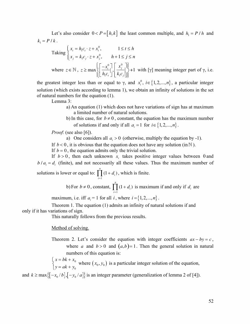
Let’s also consider [ ]0 ,P h k< = the least common multiple, and h1 = P / h and k1 = P / k .
Taking xt = h1ct ⋅ z + xt
0 , 1 ≤ t ≤ h
xj = k1cj ⋅ z + xj0 , h + 1 ≤ j ≤ n
⎧⎨⎪
⎩⎪
where z ∈N , z ≥ max−xt
0
h1ct
⎡
⎣⎢
⎤
⎦⎥ ,
x j0
k1cj
⎡
⎣⎢⎢
⎤
⎦⎥⎥
⎧⎨⎪
⎩⎪
⎫⎬⎪
⎭⎪+1 with [γ] meaning integer part of γ, i.e.
the greatest integer less than or equal to γ, and { }0 , 1,2,...,ix i n∈ , a particular integer solution (which exists according to lemma 1), we obtain an infinity of solutions in the set of natural numbers for the equation (1).
Lemma 3: a) An equation (1) which does not have variations of sign has at maximum
a limited number of natural solutions. b) In this case, for 0b ≠ , constant, the equation has the maximum number
of solutions if and only if all 1ia = for { }1,2,...,i n∈ . Proof: (see also [6]).
a) One considers all ai > 0 (otherwise, multiply the equation by -1). If 0b < , it is obvious that the equation does not have any solution (in N ). If b = 0 , the equation admits only the trivial solution. If b > 0 , then each unknown xi takes positive integer values between 0 and
b / ai = di (finite), and not necessarily all these values. Thus the maximum number of
solutions is lower or equal to: (1 + dii=1
n
∏ ) , which is finite.
b) For b ≠ 0 , constant, (1 + dii=1
n
∏ ) is maximum if and only if di are
maximum, i.e. iff ai = 1 for all i , where { }1,2,...,i n= . Theorem 1. The equation (1) admits an infinity of natural solutions if and
only if it has variations of sign. This naturally follows from the previous results. Method of solving. Theorem 2. Let’s consider the equation with integer coefficients ax − by = c ,
where a and b > 0 and a,b( )= 1 . Then the general solution in natural numbers of this equation is:
x = bk + x0
y = ak + y0
⎧⎨⎩
where ( )0 0,x y is a particular integer solution of the equation,
and [ ] [ ]{ }0 0max / , /k x b y a≥ − − is an integer parameter (generalization of lemma 2 of [4]).
53
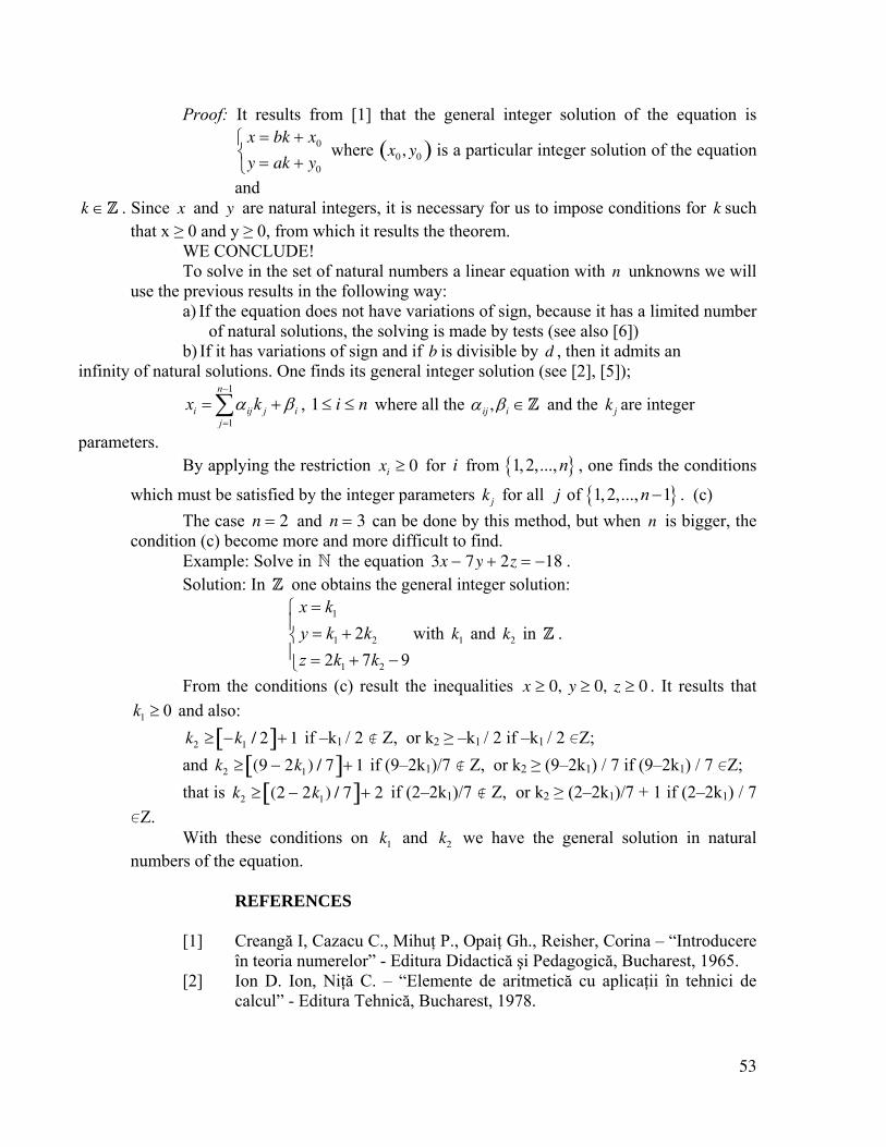
Proof: It results from [1] that the general integer solution of the equation is x = bk + x0
y = ak + y0
⎧⎨⎩
where x0 , y0( ) is a particular integer solution of the equation
and k ∈Z . Since x and y are natural integers, it is necessary for us to impose conditions for k such
that x ≥ 0 and y ≥ 0, from which it results the theorem. WE CONCLUDE! To solve in the set of natural numbers a linear equation with n unknowns we will
use the previous results in the following way: a) If the equation does not have variations of sign, because it has a limited number
of natural solutions, the solving is made by tests (see also [6]) b) If it has variations of sign and if b is divisible by d , then it admits an
infinity of natural solutions. One finds its general integer solution (see [2], [5]); 1
1
n
i ij j ij
x kα β−
=
= +∑ , 1 ≤ i ≤ n where all the α ij ,βi ∈Z and the kj are integer
parameters. By applying the restriction xi ≥ 0 for i from { }1,2,...,n , one finds the conditions
which must be satisfied by the integer parameters kj for all j of { }1,2,..., 1n − . (c) The case n = 2 and n = 3 can be done by this method, but when n is bigger, the
condition (c) become more and more difficult to find. Example: Solve in N the equation 3x − 7y + 2z = −18 . Solution: In Z one obtains the general integer solution:
1
1 2
1 2
22 7 9
x ky k kz k k
=⎧⎪ = +⎨⎪ = + −⎩
with k1 and k2 in Z .
From the conditions (c) result the inequalities x ≥ 0, y ≥ 0, z ≥ 0 . It results that
1 0k ≥ and also: k2 ≥ −k1 / 2[ ]+ 1 if –k1 / 2 ó Z, or k2 ≥ –k1 / 2 if –k1 / 2 0Z; and k2 ≥ (9 − 2k1) / 7[ ]+ 1 if (9–2k1)/7 ó Z, or k2 ≥ (9–2k1) / 7 if (9–2k1) / 7 0Z; that is k2 ≥ (2 − 2k1) / 7[ ]+ 2 if (2–2k1)/7 ó Z, or k2 ≥ (2–2k1)/7 + 1 if (2–2k1) / 7
0Z. With these conditions on k1 and k2 we have the general solution in natural
numbers of the equation.
REFERENCES
[1] Creangă I, Cazacu C., Mihuţ P., Opaiţ Gh., Reisher, Corina – “Introducere în teoria numerelor” - Editura Didactică şi Pedagogică, Bucharest, 1965.
[2] Ion D. Ion, Niţă C. – “Elemente de aritmetică cu aplicaţii în tehnici de calcul” - Editura Tehnică, Bucharest, 1978.
54
[3] Popovici C. P. – “Logica şi teoria numerelor” - Editura Didactică şi Pedagogică, Bucharest, 1970.
[4] Andrica Dorin, Andreescu Titu – “Existenţa unei soluţii de bază pentru ecuaţia ax2 − by2 = 1” - Gazeta Matematică, Nr. 2/1981.
[5] Smarandache, Florentin Gh. – “Un algorithme de résolution dans l’ensemble des nombres entiers des équations linéaires”, 1981;
a more general English version of this French article is: “Integer Algorithms to Solver Linear Equations and Systems” in arXiv at http://xxx.lanl.gov/pdf/math/0010134 ;
[6] Smarandache, Florentin Gh. – Problema E: 6919, Gazeta Matematică, Nr. 7/1980.
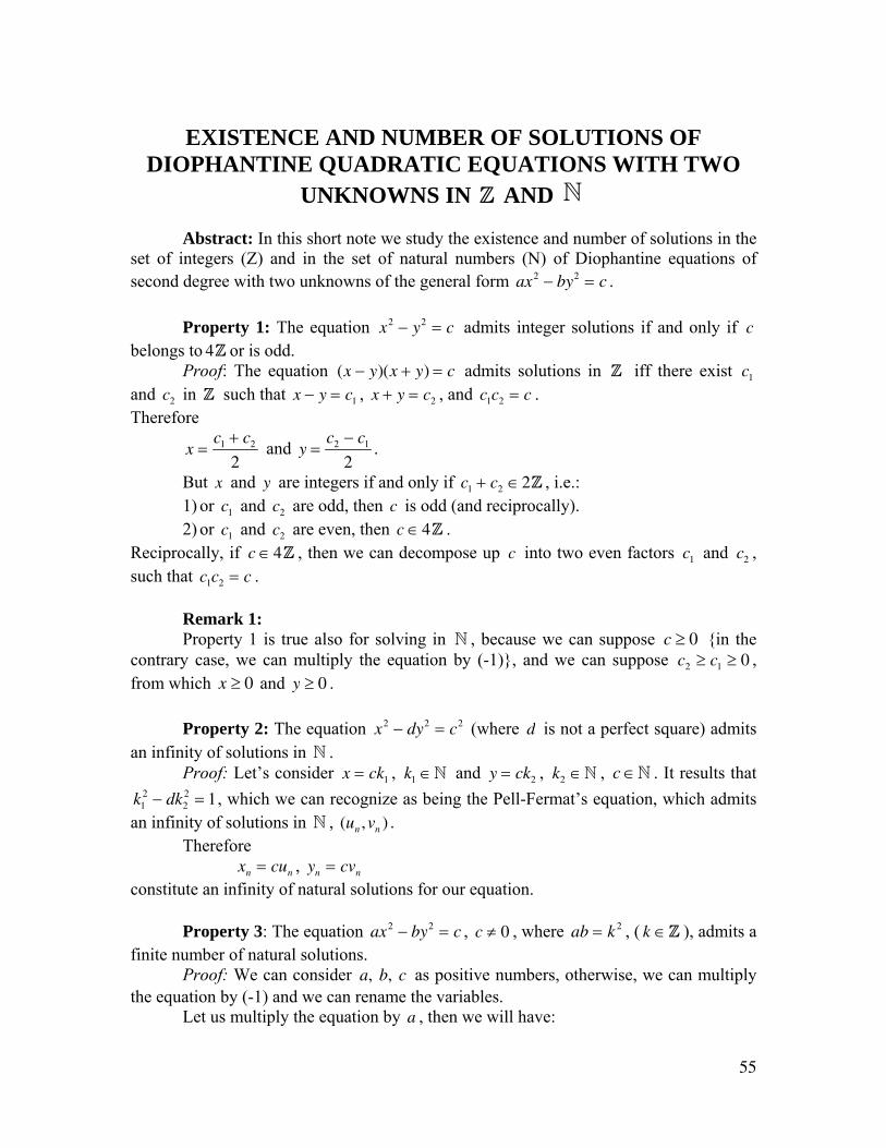
55
EXISTENCE AND NUMBER OF SOLUTIONS OF DIOPHANTINE QUADRATIC EQUATIONS WITH TWO
UNKNOWNS IN Z AND N Abstract: In this short note we study the existence and number of solutions in the
set of integers (Z) and in the set of natural numbers (N) of Diophantine equations of second degree with two unknowns of the general form ax2 − by2 = c .
Property 1: The equation x2 − y2 = c admits integer solutions if and only if c
belongs to 4Z or is odd. Proof: The equation (x − y)(x + y) = c admits solutions in Z iff there exist c1
and c2 in Z such that x − y = c1 , x + y = c2 , and c1c2 = c . Therefore
x =c1 + c2
2 and y =
c2 − c1
2.
But x and y are integers if and only if c1 + c2 ∈2Z , i.e.: 1) or c1 and c2 are odd, then c is odd (and reciprocally). 2) or c1 and c2 are even, then c ∈4Z .
Reciprocally, if c ∈4Z , then we can decompose up c into two even factors c1 and c2 , such that c1c2 = c .
Remark 1: Property 1 is true also for solving in N , because we can suppose c ≥ 0 {in the
contrary case, we can multiply the equation by (-1)}, and we can suppose c2 ≥ c1 ≥ 0 , from which x ≥ 0 and y ≥ 0 .
Property 2: The equation x2 − dy2 = c2 (where d is not a perfect square) admits
an infinity of solutions in N . Proof: Let’s consider x = ck1 , k1 ∈N and y = ck2 , k2 ∈N , c ∈N . It results that
k12 − dk2
2 = 1, which we can recognize as being the Pell-Fermat’s equation, which admits an infinity of solutions in N , (un ,vn ) .
Therefore xn = cun , yn = cvn
constitute an infinity of natural solutions for our equation. Property 3: The equation ax2 − by2 = c , c ≠ 0 , where ab = k 2 , ( k ∈Z ), admits a
finite number of natural solutions. Proof: We can consider a, b, c as positive numbers, otherwise, we can multiply
the equation by (-1) and we can rename the variables. Let us multiply the equation by a , then we will have:
56
z2 − t 2 = d with z = ax ∈N , t = ky ∈N and d = ac > 0 . (1) We will solve it as in property 1, which gives z and t .
But in (1) there is a finite number of natural solutions, because there is a finite number of integer divisors for a number in N
* . Because the pairs (z,t) are in a limited number, it results that the pairs (z / a, t / k) also are in a limited number, and the same for the pairs (x, y) .
Property 4: If ax2 − by2 = c , where ab ≠ k 2 ( k ∈Z ) admits a particular nontrivial solution in N , then it admits an infinity of solutions in N .
Proof: Let’s consider:
xn = x0un + by0vn
yn = y0un + ax0vn
⎧⎨⎩
(n ∈N) (2)
where (x0 , y0 ) is the particular natural solution for the initial equation, and (un ,vn )n∈N is the general natural solution for the equation u2 − abv2 = 1 , called the solution Pell, which admits an infinity of solutions.
Then axn2 − byn
2 = (ax02 − by0
2 )(un2 − abvn
2 ) = c . Therefore (2) verifies the initial equation.
[1982]
57
CONVERGENCE OF A FAMILY OF SERIES In this article we will construct a family of expressionsε(n) . For each element
E(n) from ε(n) , the convergence of the series ( )En n
E n≥∑ could be determined in
accordance to the theorems from this article. This article gives also applications.
(1) Preliminary
To render easier the expression, we will use the recursive functions. We will introduce some notations and notions to simplify and reduce the size of this article.
(2) Definitions: lemmas.
We will construct recursively a family of expressions ε(n) . For each expression E(n) ∈ε(n) , the degree of the expression is defined recursively and
is denoted 0 ( )d E n , and its dominant (leading) coefficient is denoted c(E(n)) . 1. If a is a real constant, then a ∈ε(n) .
d 0a = 0 and c(a) = a . 2. The positive integer n ∈ε(n) .
d 0n = 1 and c(n) = 1.
3. If E1(n) and E2 (n) belong to ε(n) with d 0E1(n) = r1 and
d 0E2 (n) = r2 , c(E1(n)) = a1 and c(E2 (n)) = a2 , then:
a) E1(n)E2 (n) ∈ε (n) ; d 0 (E1(n)E2 (n)) = r1 + r2 ; c(E1(n)E2 (n)) which is a1a2 .
b) If E2 (n) ≠ 0 ∀n ∈N(n ≥ nE2) , then
E1(n)
E2 (n)∈ε(n) and
d0 E1(n)
E2 (n)
⎛⎝⎜
⎞⎠⎟
= r1 − r2 , cE1(n)
E2 (n)
⎛⎝⎜
⎞⎠⎟
=a1
a2
.
c) If α is a real constant and if the operation used is well defined,
E1(n)( )α (for all
1 , En N n n∈ ≥ ), then:
( )1( ) ( )E n nα ε∈ , ( )( )01 1( )d E n rα α= , ( )( )1 1( )c E n aα α=
d) If r1 ≠ r2 , then E1(n) ± E2 (n) ∈ε(n) , d 0 E1(n) ± E2 (n)( ) is the max
of r1 and r2 , and c E1(n) ± E2 (n)( )= a1 , respectively a2 resulting
that the grade is r1 and r2 . e) If r1 = r2 and a1 + a2 ≠ 0 , then E1(n) + E2 (n) ∈ε (n) ,
d 0 E1(n) + E2 (n)( )= r1 and c E1(n) + E2 (n)( )= a1 + a2 .
58
f) If r1 = r2 and a1 − a2 ≠ 0 , then E1(n) − E2 (n) ∈ε (n) ,
d 0 E1(n) − E2 (n)( )= r1 and c E1(n) − E2 (n)( )= a1 − a2 . 4. All expressions obtained by applying a finite number of step 3 belong
to ε (n) .
Note 1. From the definition of ε (n) it results that, if E(n) ∈ε (n) then
c E(n)( )≠ 0 , and that c E(n)( )= 0 if and only if E(n) = 0 . Lemma 1. If E(n) ∈ε(n) and c E(n)( )> 0 , then there exists n
' ∈N , such that for
all n > n ' , E(n) > 0 .
Proof: Let’s consider c E(n)( )= a1 > 0 and d 0 E(n)( )= r .
If r > 0 , then 1( )lim ( ) lim limr r
rn n n
E nE n n a nn→∞ →∞ →∞
= = = +∞ , thus there exists
n' ∈N such that, for any n > n ' we have E(n) > 0 .
If r < 0 , then 1
1 1lim lim lim( )( )
rr
n n n
r
n nE nE n an
−−
→∞ →∞ →∞= = = +∞ thus there exists
n' ∈N , such that for all n > n ' ,
1
E(n)> 0 we have E(n) > 0 .
If r = 0 , then E(n) is a positive real constant, or E1(n)
E2 (n)= E(n) , with
d 0E1(n) = d 0E2 (n) = r1 ≠ 0 , according to what we have just seen,
cE1(n)
E2 (n)
⎛⎝⎜
⎞⎠⎟
=c E1(n)( )c E2 (n)( )= c E(n)( )> 0 .
Then: c E1(n)( )> 0 and c E2 (n)( )< 0 : it results
1 1
2 2
1
2
there exists , and , ( ) 0
there exists , and , ( ) 0E E
E E
n n n n E n
n n n n E n
∈ ∀ ∈ ≥ > ⎫⎪ ⇒⎬∈ ∀ ∈ ≥ > ⎪⎭
N NN N
1 2
1
2
( )there exists max( , ) , , , ( ) 0( )E E E E
E nn n n n n n E nE n
= ∈ ∀ ∈ ≥ >N N
then ( )1( ) 0c E n < and c E2 (n)( )< 0 and it results:
E(n) =E1(n)
E2 (n)=
−E1(n)
−E2 (n) which brings us back to the precedent case.
Lemma 2: If E(n) ∈ε(n) and if c E(n)( )< 0 , then it exists n
' ∈N , such that for
any n > n ' , E(n) < 0 . Proof:
59
The expression −E(n) has the propriety that c −E(n)( )> 0 , according to the
recursive definition. According to lemma 1: there exists n' ∈N , n ≥ n ' , −E(n) > 0 , i.e.
+E(n) < 0 , q. e. d. Note 2. To prove the following theorem, we suppose known the criterion of
convergence of the series and certain of its properties
(3) Theorem of convergence and applications. Theorem: Let’s consider ( ) ( )E n nε∈ with d 0 E(n)( )= r having the series
E(n)n≥nε
∑ , E(n) /≡ 0 .
Then: A) If r < −1 the series is absolutely convergent. B) If r ≥ −1 it is divergent where E(n) is well defined ∀n ≥ nE ,n ∈N .
Proof: According to lemmas 1 and 2, and because:
the series ( )En n
E n≥∑ converge ⇔ the series ( )
En nE n
≥
−∑ converge,
we can consider the series ( )En n
E n≥∑ like a series with positive terms.
We will prove that the series ( )En n
E n≥∑ has the same nature as the series
1
n−rn≥1∑ .
Let us apply the second criterion of comparison:
( )( ) ( )lim lim ( )1 rn n
r
E n E n c E nn
n→∞ →∞
−
= = ≠ ±∞ .
According to the note 1 if E(n) /≡ 0 then c E(n)( )≠ 0 and then the series ( )En n
E n≥∑ has
the same nature as the series 1
n−rn≥1∑ , i.e.:
A) If r < −1 then the series is convergent; B) If r > −1 then the series is divergent; For r < −1 the series is absolute convergent because it is a series with
positive terms.
Applications: We can find many applications of these. Here is an interesting one: If Pq (n) , Rs (n) are polynomials of n of degree q, s , and that Pq (n) and Rs (n)
belong to ε (n) :
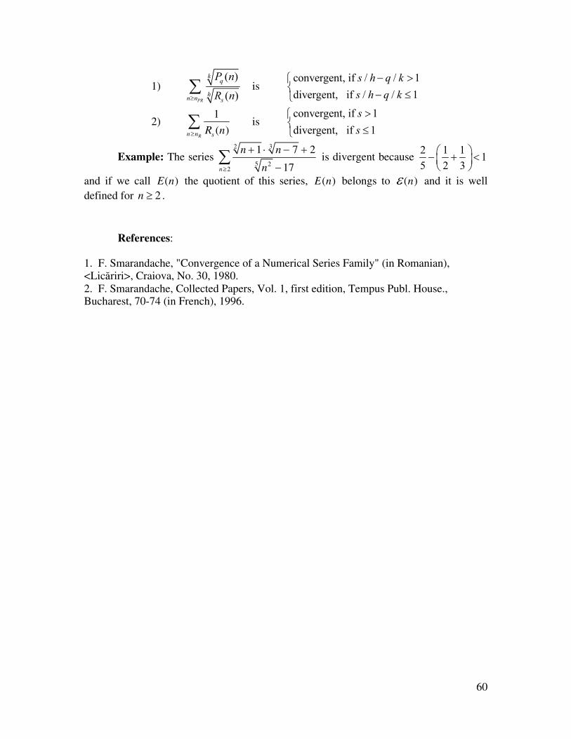
60
1) ( )
( )PR
kq
hn n s
P n
R n≥∑ is
convergent, if / / 1divergent, if / / 1
s h q ks h q k
− >⎧⎨ − ≤⎩
2) 1
Rs (n)n≥nR
∑ is convergent, if 1divergent, if 1
ss
>⎧⎨ ≤⎩
Example: The series n + 12 ⋅ n − 73 + 2
n25 − 17n≥2∑ is divergent because
2 1 1 15 2 3
⎛ ⎞− + <⎜ ⎟⎝ ⎠
and if we call E(n) the quotient of this series, E(n) belongs to ε (n) and it is well defined for n ≥ 2 .
References:
1. F. Smarandache, "Convergence of a Numerical Series Family" (in Romanian), <Lic|riri>, Craiova, No. 30, 1980. 2. F. Smarandache, Collected Papers, Vol. 1, first edition, Tempus Publ. House., Bucharest, 70-74 (in French), 1996.
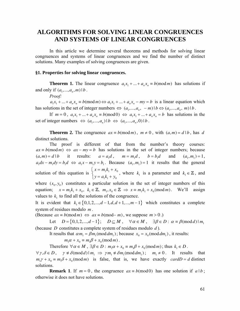
61
ALGORITHMS FOR SOLVING LINEAR CONGRUENCES AND SYSTEMS OF LINEAR CONGRUENCES
In this article we determine several theorems and methods for solving linear congruences and systems of linear congruences and we find the number of distinct solutions. Many examples of solving congruences are given.
§1. Properties for solving linear congruences. Theorem 1. The linear congruence a1x1 + ... + anxn ≡ b(mod m) has solutions if and only if (a1,...,an , m) | b . Proof: a1x1 + ... + anxn ≡ b(mod m) ⇔ a1x1 + ... + anxn − my = b is a linear equation which has solutions in the set of integer numbers ⇔ (a1,...,an , − m) | b ⇔ (a1,...,an , m) | b . If m = 0 , a1x1 + ... + anxn ≡ b(mod 0) ⇔ a1x1 + ... + anxn = b has solutions in the set of integer numbers ⇔ (a1,...,an ) | b ⇔ (a1,...,an ,0) | b . Theorem 2. The congruence ax ≡ b(mod m) , m ≠ 0 , with (a, m) = d | b , has d distinct solutions. The proof is different of that from the number’s theory courses: ax ≡ b(mod m) ⇔ ax − my = b has solutions in the set of integer numbers; because (a, m) = d | b it results: a = a1d , m = m1d , b = b1d and (a1, m1) = 1, a1dx − m1dy = b1d ⇔ a1x − m1y = b1 . Because (a1, m1) = 1 it results that the general
solution of this equation is x = m1k1 + x0
y = a1k1 + y0
⎧⎨⎩
, where k1 is a parameter and k1 ∈Z , and
where (x0 , y0 ) constitutes a particular solution in the set of integer numbers of this equation; x = m1k1 + x0 , k1 ∈Z, m1, x0 ∈Z ⇒ x ≡ m1k1 + x0 (mod m) . We’ll assign values to k1 to find all the solutions of the congruence. It is evident that k1 ∈ 0,1,2,...,d − 1,d,d + 1,..., m − 1{ } which constitutes a complete system of residues modulo m . (Because ax ≡ b(mod m) ⇔ ax ≡ b(mod− m) , we suppose m > 0 .) Let D = 0,1,2,...,d − 1{ }; D ⊆ M , ∀α ∈M , ∃β ∈D : α ≡ β(mod d) | m1 (because D constitutes a complete system of residues modulo d ). It results that αm1 = βm1(mod dm1) ; because x0 = x0 (mod dm1) , it results:
m1α + x0 ≡ m1β + x0 (mod m) . Therefore ∀α ∈M , ∃β ∈D : m1α + x0 ≡ m1β + x0 (mod m) ; thus k1 ∈D . ∀γ ,δ ∈D , γ /≡ δ (mod d) | m1 ⇒ γ m1 /≡ δm1(mod dm1) ; m1 ≠ 0 . It results that m1γ + x0 ≡ m1δ + x0 (mod m) is false, that is, we have exactly cardD = d distinct solutions. Remark 1. If m = 0 , the congruence ax ≡ b(mod 0) has one solution if a | b ; otherwise it does not have solutions.
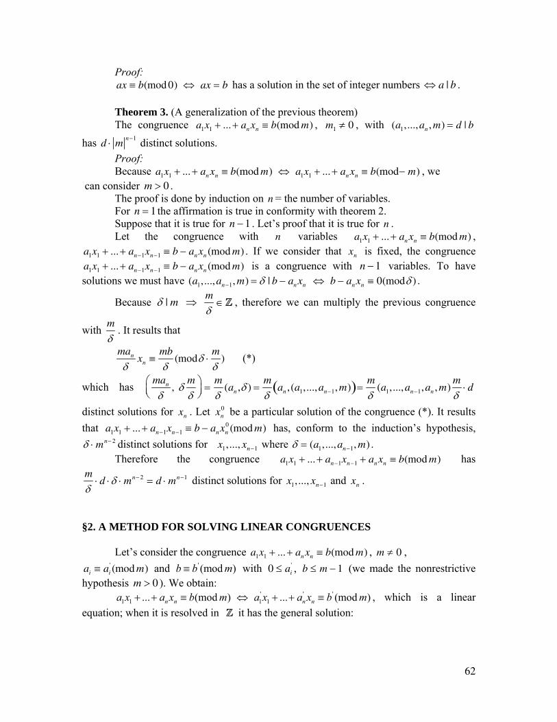
62
Proof: ax ≡ b(mod 0) ⇔ ax = b has a solution in the set of integer numbers ⇔ a | b . Theorem 3. (A generalization of the previous theorem) The congruence a1x1 + ... + an xn ≡ b(mod m) , m1 ≠ 0 , with (a1,...,an , m) = d | b
has d ⋅ mn−1 distinct solutions.
Proof: Because a1x1 + ... + anxn ≡ b(mod m) ⇔ a1x1 + ... + anxn ≡ b(mod− m) , we can consider m > 0 . The proof is done by induction on n = the number of variables. For n = 1 the affirmation is true in conformity with theorem 2. Suppose that it is true for n − 1 . Let’s proof that it is true for n . Let the congruence with n variables a1x1 + ... + anxn ≡ b(mod m) , a1x1 + ... + an−1xn−1 ≡ b − anxn (mod m) . If we consider that xn is fixed, the congruence a1x1 + ... + an−1xn−1 ≡ b − anxn (mod m) is a congruence with n − 1 variables. To have solutions we must have (a1,...,an−1, m) = δ | b − anxn ⇔ b − anxn ≡ 0(modδ ) .
Because δ | m ⇒ m
δ∈Z , therefore we can multiply the previous congruence
with m
δ. It results that
man
δxn ≡
mb
δ(modδ ⋅
m
δ) (*)
which has man
δ, δ
m
δ⎛⎝⎜
⎞⎠⎟
=m
δ(an ,δ ) =
m
δan ,(a1,...,an−1, m)( )=
m
δ(a1,...,an−1,an , m)
m
δ⋅ d
distinct solutions for xn . Let xn0 be a particular solution of the congruence (*). It results
that a1x1 + ... + an−1xn−1 ≡ b − anxn0 (mod m) has, conform to the induction’s hypothesis,
δ ⋅ mn− 2 distinct solutions for x1,..., xn−1 where δ = (a1,...,an−1, m) . Therefore the congruence a1x1 + ... + an−1xn−1 + anxn ≡ b(mod m) has m
δ⋅ d ⋅δ ⋅ mn− 2 = d ⋅ mn−1 distinct solutions for x1,..., xn−1 and xn .
§2. A METHOD FOR SOLVING LINEAR CONGRUENCES
Let’s consider the congruence a1x1 + ... + an xn ≡ b(mod m) , m ≠ 0 , ai ≡ ai
' (mod m) and ' (mod )b b m≡ with 0 ≤ ai' , b ≤ m − 1 (we made the nonrestrictive
hypothesis m > 0 ). We obtain: ' ' '
1 1 1 1... (mod ) ... (mod )n n n na x a x b m a x a x b m+ + ≡ ⇔ + + ≡ , which is a linear equation; when it is resolved in Z it has the general solution:
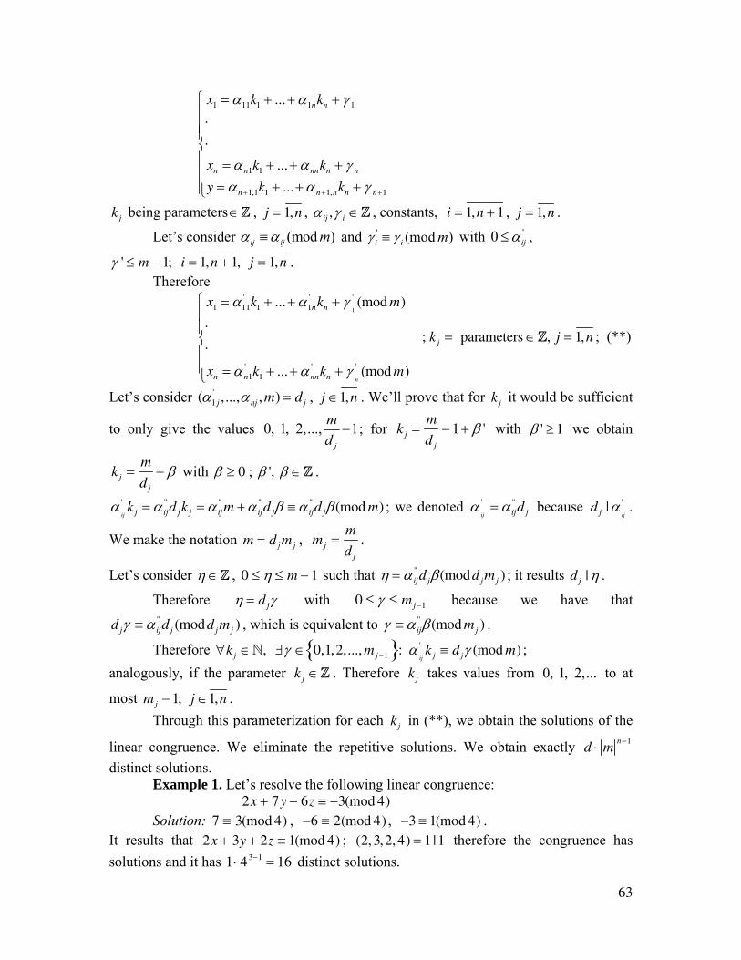
63
x1 = α11k1 + ...+ α1nkn + γ 1
⋅⋅xn = αn1k1 + ...+ αnnkn + γ n
y = αn+1,1k1 + ...+ αn+1,nkn + γ n+1
⎧
⎨
⎪⎪⎪
⎩
⎪⎪⎪
kj being parameters ∈Z , j = 1,n , α ij ,γ i ∈Z , constants, i = 1,n + 1 , j = 1,n .
Let’s consider ' (mod )ij ij mα α≡ and ' (mod )i i mγ γ≡ with '0 ijα≤ ,
γ ' ≤ m − 1; i = 1,n + 1, j = 1,n . Therefore
x1 = α11' k1 + ... + α1n
' kn + γ1
' (mod m)
⋅⋅
xn = αn1' k1 + ... + αnn
' kn + γn
' (mod m)
⎧
⎨
⎪⎪
⎩
⎪⎪
; k j = parameters ∈Z, j = 1,n ; (**)
Let’s consider (α1 j' ,...,αnj
' ,m) = dj , j ∈1,n . We’ll prove that for kj it would be sufficient
to only give the values 0, 1, 2,..., 1j
md
− ; for kj =m
dj
− 1 + β ' with β ' ≥ 1 we obtain
kj =m
dj
+ β with β ≥ 0 ; β ', β ∈Z .
αij
' k j = α ij'' d jk j = α ij
'' m + α ij'' djβ ≡ α ij
'' d jβ(mod m) ; we denoted αij
' = α ij'' dj because dj | α
ij
' .
We make the notation m = djmj , mj =m
dj
.
Let’s consider η ∈Z , 0 ≤ η ≤ m − 1 such that η = α ij'' djβ(moddjmj ) ; it results dj | η .
Therefore η = djγ with 0 ≤ γ ≤ mj −1 because we have that
djγ ≡ α ij'' dj (moddjmj ) , which is equivalent to γ ≡ α ij
'' β(mod mj ) .
Therefore ∀k j ∈N, ∃γ ∈ 0,1,2,..., mj −1{ }: αij
' k j ≡ d jγ (mod m) ; analogously, if the parameter kj ∈Z . Therefore kj takes values from 0, 1, 2,... to at
most mj − 1; j ∈1,n . Through this parameterization for each kj in (**), we obtain the solutions of the
linear congruence. We eliminate the repetitive solutions. We obtain exactly d ⋅ mn−1
distinct solutions. Example 1. Let’s resolve the following linear congruence:
2x + 7y − 6z ≡ −3(mod 4) Solution: 7 ≡ 3(mod 4) , −6 ≡ 2(mod 4) , −3 ≡ 1(mod 4) . It results that 2x + 3y + 2z ≡ 1(mod 4) ; (2, 3,2, 4) = 1 |1 therefore the congruence has solutions and it has 1 ⋅ 43−1 = 16 distinct solutions.
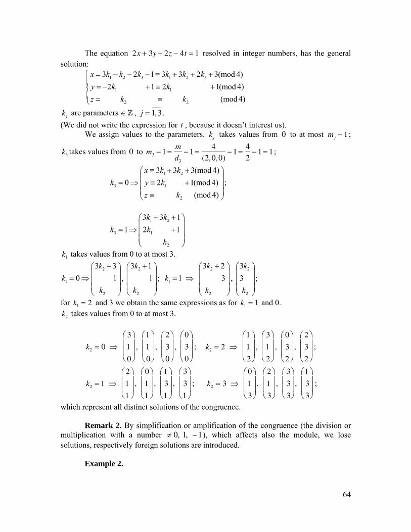
64
The equation 2x + 3y + 2z − 4t = 1 resolved in integer numbers, has the general solution:
1 2 3 1 2 3
1 1
2 2
3 2 1 3 3 2 3(mod 4)2 1 2 1(mod 4)
(mod 4)
x k k k k k ky k kz k k
= − − − ≡ + + +⎧⎪ = − + ≡ +⎨⎪ = ≡⎩
kj are parameters ∈Z , j = 1, 3 . (We did not write the expression for t , because it doesn’t interest us). We assign values to the parameters. kj takes values from 0 to at most mj − 1 ;
k3 takes values from 0 to m3 − 1 =m
d3
− 1 =4
(2,0,0)− 1 =
4
2− 1 = 1 ;
1 2
3 1
2
3 3 3(mod 4)0 2 1(mod 4)
(mod 4)
x k kk y k
z k
≡ + +⎛ ⎞⎜ ⎟= ⇒ ≡ +⎜ ⎟⎜ ⎟≡⎝ ⎠
;
1 2
3 1
2
3 3 11 2 1
k kk k
k
+ +⎛ ⎞⎜ ⎟= ⇒ +⎜ ⎟⎜ ⎟⎝ ⎠
k1 takes values from 0 to at most 3.
2
1
2
3 30 1
kk
k
+⎛ ⎞⎜ ⎟= ⇒ ⎜ ⎟⎜ ⎟⎝ ⎠
, 2
2
3 1 1
k
k
+⎛ ⎞⎜ ⎟⎜ ⎟⎜ ⎟⎝ ⎠
; 2
1
2
3 21 3
kk
k
+⎛ ⎞⎜ ⎟= ⇒ ⎜ ⎟⎜ ⎟⎝ ⎠
, 2
2
33k
k
⎛ ⎞⎜ ⎟⎜ ⎟⎜ ⎟⎝ ⎠
;
for k1 = 2 and 3 we obtain the same expressions as for k1 = 1 and 0. k2 takes values from 0 to at most 3.
k2 = 0 ⇒
3
1
0
⎛
⎝
⎜⎜
⎞
⎠
⎟⎟
,
1
1
0
⎛
⎝
⎜⎜
⎞
⎠
⎟⎟
,
2
3
0
⎛
⎝
⎜⎜
⎞
⎠
⎟⎟
,
0
3
0
⎛
⎝
⎜⎜
⎞
⎠
⎟⎟
; k2 = 2 ⇒
1
1
2
⎛
⎝
⎜⎜
⎞
⎠
⎟⎟
,
3
1
2
⎛
⎝
⎜⎜
⎞
⎠
⎟⎟
,
0
3
2
⎛
⎝
⎜⎜
⎞
⎠
⎟⎟
,
2
3
2
⎛
⎝
⎜⎜
⎞
⎠
⎟⎟
;
k2 = 1 ⇒
2
1
1
⎛
⎝
⎜⎜
⎞
⎠
⎟⎟
,
0
1
1
⎛
⎝
⎜⎜
⎞
⎠
⎟⎟
,
1
3
1
⎛
⎝
⎜⎜
⎞
⎠
⎟⎟
,
3
3
1
⎛
⎝
⎜⎜
⎞
⎠
⎟⎟
; k2 = 3 ⇒
0
1
3
⎛
⎝
⎜⎜
⎞
⎠
⎟⎟
,
2
1
3
⎛
⎝
⎜⎜
⎞
⎠
⎟⎟
,
3
3
3
⎛
⎝
⎜⎜
⎞
⎠
⎟⎟
,
1
3
3
⎛
⎝
⎜⎜
⎞
⎠
⎟⎟
;
which represent all distinct solutions of the congruence. Remark 2. By simplification or amplification of the congruence (the division or multiplication with a number ≠ 0, 1, −1), which affects also the module, we lose solutions, respectively foreign solutions are introduced. Example 2.
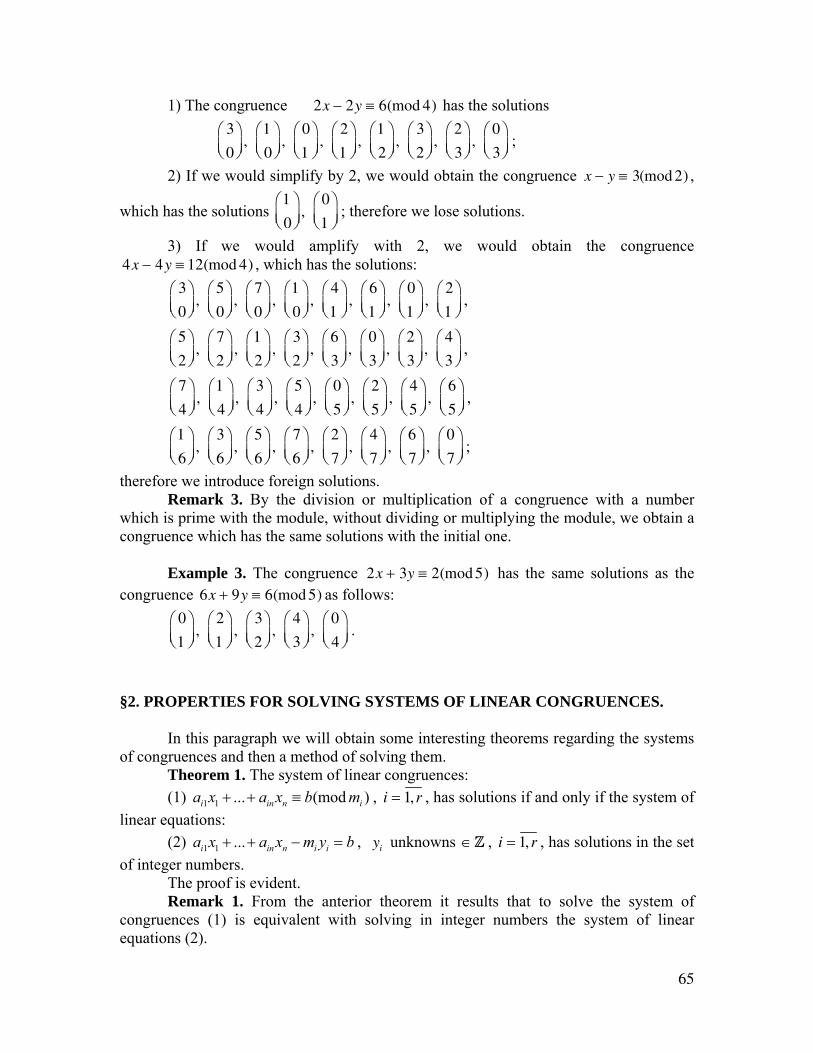
65
1) The congruence 2x − 2y ≡ 6(mod 4) has the solutions 3
0
⎛⎝⎜
⎞⎠⎟
, 1
0
⎛⎝⎜
⎞⎠⎟
, 0
1
⎛⎝⎜
⎞⎠⎟
, 2
1
⎛⎝⎜
⎞⎠⎟
, 1
2
⎛⎝⎜
⎞⎠⎟
, 3
2
⎛⎝⎜
⎞⎠⎟
, 2
3
⎛⎝⎜
⎞⎠⎟
, 0
3
⎛⎝⎜
⎞⎠⎟
;
2) If we would simplify by 2, we would obtain the congruence x − y ≡ 3(mod 2) ,
which has the solutions 1
0
⎛⎝⎜
⎞⎠⎟
, 0
1
⎛⎝⎜
⎞⎠⎟
; therefore we lose solutions.
3) If we would amplify with 2, we would obtain the congruence 4x − 4y ≡ 12(mod 4) , which has the solutions:
3
0
⎛⎝⎜
⎞⎠⎟
, 5
0
⎛⎝⎜
⎞⎠⎟
, 7
0
⎛⎝⎜
⎞⎠⎟
, 1
0
⎛⎝⎜
⎞⎠⎟
, 4
1
⎛⎝⎜
⎞⎠⎟
, 6
1
⎛⎝⎜
⎞⎠⎟
, 0
1
⎛⎝⎜
⎞⎠⎟
, 2
1
⎛⎝⎜
⎞⎠⎟
,
5
2
⎛⎝⎜
⎞⎠⎟
, 7
2
⎛⎝⎜
⎞⎠⎟
, 1
2
⎛⎝⎜
⎞⎠⎟
, 3
2
⎛⎝⎜
⎞⎠⎟
, 6
3
⎛⎝⎜
⎞⎠⎟
, 0
3
⎛⎝⎜
⎞⎠⎟
, 2
3
⎛⎝⎜
⎞⎠⎟
, 4
3
⎛⎝⎜
⎞⎠⎟
,
7
4
⎛⎝⎜
⎞⎠⎟
, 1
4
⎛⎝⎜
⎞⎠⎟
, 3
4
⎛⎝⎜
⎞⎠⎟
, 5
4
⎛⎝⎜
⎞⎠⎟
, 0
5
⎛⎝⎜
⎞⎠⎟
, 2
5
⎛⎝⎜
⎞⎠⎟
, 4
5
⎛⎝⎜
⎞⎠⎟
, 6
5
⎛⎝⎜
⎞⎠⎟
,
1
6
⎛⎝⎜
⎞⎠⎟
, 3
6
⎛⎝⎜
⎞⎠⎟
, 5
6
⎛⎝⎜
⎞⎠⎟
, 7
6
⎛⎝⎜
⎞⎠⎟
, 2
7
⎛⎝⎜
⎞⎠⎟
, 4
7
⎛⎝⎜
⎞⎠⎟
, 6
7
⎛⎝⎜
⎞⎠⎟
, 0
7
⎛⎝⎜
⎞⎠⎟
;
therefore we introduce foreign solutions. Remark 3. By the division or multiplication of a congruence with a number which is prime with the module, without dividing or multiplying the module, we obtain a congruence which has the same solutions with the initial one. Example 3. The congruence 2x + 3y ≡ 2(mod 5) has the same solutions as the congruence 6x + 9y ≡ 6(mod 5) as follows:
0
1
⎛⎝⎜
⎞⎠⎟
, 2
1
⎛⎝⎜
⎞⎠⎟
, 3
2
⎛⎝⎜
⎞⎠⎟
, 4
3
⎛⎝⎜
⎞⎠⎟
, 0
4
⎛⎝⎜
⎞⎠⎟
.
§2. PROPERTIES FOR SOLVING SYSTEMS OF LINEAR CONGRUENCES. In this paragraph we will obtain some interesting theorems regarding the systems of congruences and then a method of solving them. Theorem 1. The system of linear congruences:
(1) 1 1 ... (mod )i in n ia x a x b m+ + ≡ , i = 1,r , has solutions if and only if the system of linear equations:
(2) 1 1 ...i in n i ia x a x m y b+ + − = , yi unknowns ∈Z , i = 1,r , has solutions in the set of integer numbers.
The proof is evident. Remark 1. From the anterior theorem it results that to solve the system of
congruences (1) is equivalent with solving in integer numbers the system of linear equations (2).
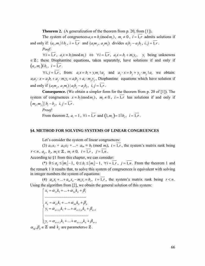
66
Theorem 2. (A generalization of the theorem from p. 20, from [1]). The system of congruences aix ≡ bi (mod mi ) , mi ≠ 0 , i = 1,r admits solutions if
and only if: (ai , mi ) | bi , i = 1,r and ( , )i j j ia m a m divides aibj − ajbi , i, j = 1,r . Poof: ∀i = 1,r , aix ≡ bi (mod mi ) ⇔ ∀i = 1,r , aix = bi + mi yi , yi being unknowns
∈Z ; these Diophantine equations, taken separately, have solutions if and only if ai , mi( )| bi , i = 1,r .
∀i, j = 1,r , from: ai x = bi + yimi | aj and aj ⋅ x = bj + yj ⋅ mj | ai we obtain: aiaj ⋅ x = ajbi + aj ⋅ mi yi = aibj + ai ⋅ mj yj , Diophantine equations which have solution if
and only if ( , ) |i j j i i j j ia m a m a b a b− , i, j = 1,r . Consequence. (We obtain a simpler form for the theorem from p. 20 of [1]). The
system of congruences x ≡ bi (mod mi ) , mi ≠ 0 , i = 1,r has solutions if and only if
( ), |i j i jm m b b− , i, j = 1,r . Proof: From theorem 2, ai = 1 , ∀i = 1,r and 1, mi( )= 1 | bi , i = 1,r .
§4. METHOD FOR SOLVING SYSTEMS OF LINEAR CONGRUENCES Let’s consider the system of linear congruences: (3) ai1x1 + ai2x2 +…+ ain ≡ bi (mod mi), i = 1,r , the system’s matrix rank being r < n , , , ij i ia b m ∈Z , mi ≠ 0, i = 1,r , j = 1,n . According to §1 from this chapter, we can consider: (*) 0 1ij ia m≤ ≤ − , 0 ≤ bi ≤ mi − 1, ∀i = 1,r , j = 1,n . From the theorem 1 and the remark 1 it results that, to solve this system of congruences is equivalent with solving in integer numbers the system of equations:
(4) 1 1 ...i in n i i ia x a x m y b+ + − = , i = 1,r , the system’s matrix rank being r < n . Using the algorithm from [2], we obtain the general solution of this system:
x1 = α11k1 + ...+ α1nkn + β1
.........................................
xn = αn1k1 + ...+ αnnkn + βn
y1 = αn+1,1k1 + ...+ αn+1,nkn + βn+1
...........................................
yr = αn+ r ,1k1 + ...+ αn+ r ,nkn + βn+ r
⎧
⎨
⎪⎪⎪
⎩
⎪⎪⎪⎪
αhj ,βh ∈Z and kj are parameters ∈Z .
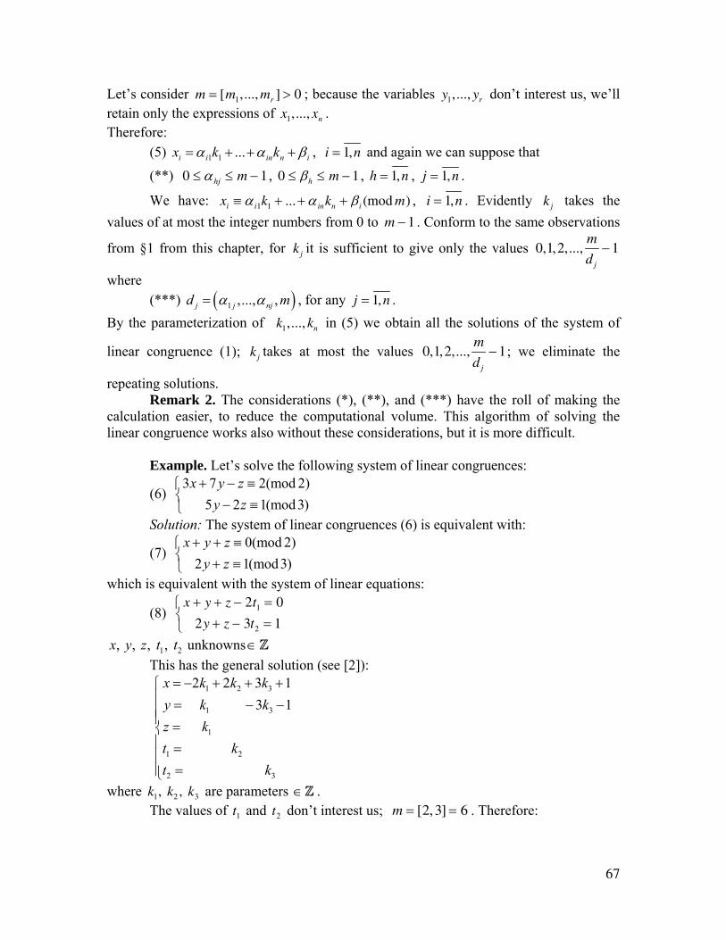
67
Let’s consider m = [m1,..., mr ] > 0 ; because the variables y1,..., yr don’t interest us, we’ll retain only the expressions of x1,..., xn . Therefore: (5) 1 1 ...i i in n ix k kα α β= + + + , i = 1,n and again we can suppose that
(**) 0 ≤ αhj ≤ m − 1 , 0 ≤ βh ≤ m − 1 , h = 1,n , j = 1,n .
We have: xi ≡ α i1k1 + ... + α inkn + βi (mod m) , i = 1,n . Evidently kj takes the values of at most the integer numbers from 0 to m − 1 . Conform to the same observations
from §1 from this chapter, for kj it is sufficient to give only the values 0,1,2,...,m
dj
− 1
where (***) ( )1 ,..., ,j j njd mα α= , for any j = 1,n .
By the parameterization of k1,..., kn in (5) we obtain all the solutions of the system of
linear congruence (1); kj takes at most the values 0,1,2,...,m
dj
− 1; we eliminate the
repeating solutions. Remark 2. The considerations (*), (**), and (***) have the roll of making the
calculation easier, to reduce the computational volume. This algorithm of solving the linear congruence works also without these considerations, but it is more difficult.
Example. Let’s solve the following system of linear congruences:
(6) 3 7 2(mod 2) 5 2 1(mod 3)x y z
y z+ − ≡⎧
⎨ − ≡⎩
Solution: The system of linear congruences (6) is equivalent with:
(7) 0(mod 2)
2 1(mod3)x y z
y z+ + ≡⎧
⎨ + ≡⎩
which is equivalent with the system of linear equations:
(8) x + y + z − 2t1 = 0
2y + z − 3t2 = 1
⎧⎨⎩
1 2, , , , unknownsx y z t t ∈Z This has the general solution (see [2]):
1 2 3
1 3
1
1 2
2 3
2 2 3 1 3 1
x k k ky k kz kt kt k
= − + + +⎧⎪ = − −⎪⎪ =⎨⎪ =⎪⎪ =⎩
where k1, k2 , k3 are parameters ∈Z . The values of t1 and t2 don’t interest us; m = [2,3] = 6 . Therefore:
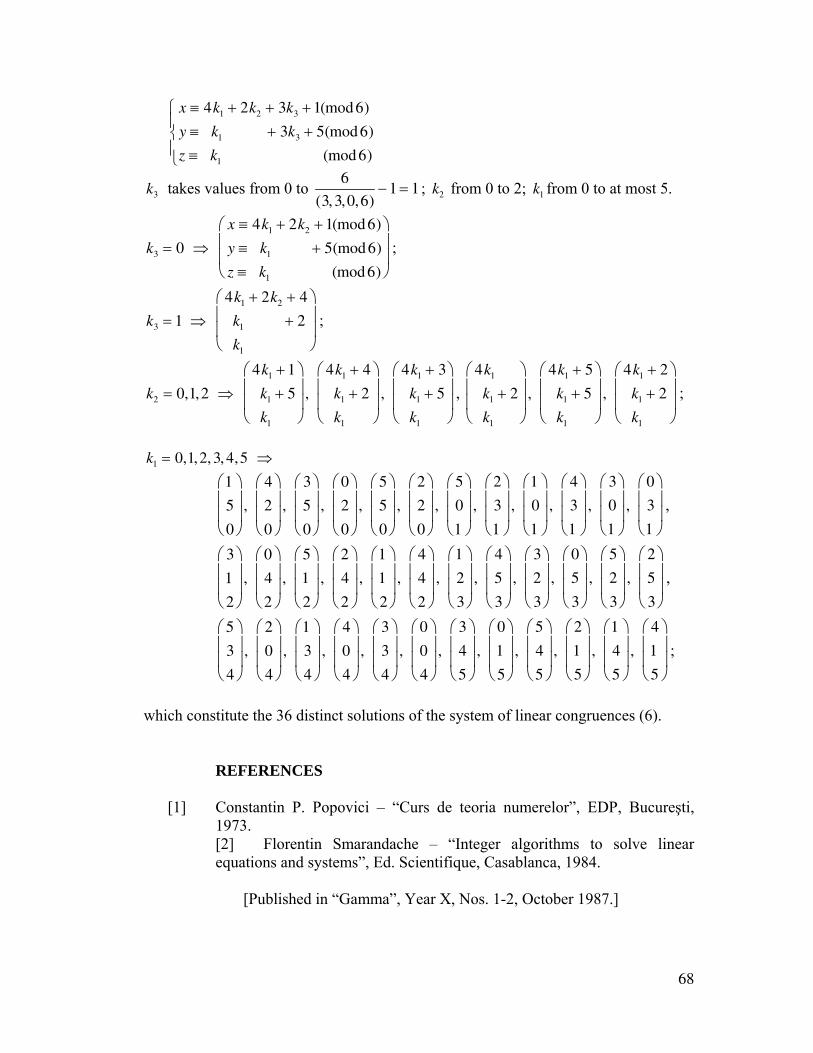
68
x ≡ 4k1 + 2k2 + 3k3 + 1(mod 6)
y ≡ k1 + 3k3 + 5(mod 6)
z ≡ k1 (mod 6)
⎧
⎨⎪
⎩⎪
k3 takes values from 0 to 6
(3,3,0,6)− 1 = 1 ; k2 from 0 to 2; k1 from 0 to at most 5.
k3 = 0 ⇒
x ≡ 4k1 + 2k2 + 1(mod 6)
y ≡ k1 + 5(mod 6)
z ≡ k1 (mod 6)
⎛
⎝
⎜⎜
⎞
⎠
⎟⎟
;
k3 = 1 ⇒
4k1 + 2k2 + 4
k1 + 2
k1
⎛
⎝
⎜⎜
⎞
⎠
⎟⎟
;
k2 = 0,1,2 ⇒
4k1 + 1
k1 + 5
k1
⎛
⎝
⎜⎜
⎞
⎠
⎟⎟
,
4k1 + 4
k1 + 2
k1
⎛
⎝
⎜⎜
⎞
⎠
⎟⎟
,
4k1 + 3
k1 + 5
k1
⎛
⎝
⎜⎜
⎞
⎠
⎟⎟
, 4k1
k1 + 2
k1
⎛
⎝
⎜⎜
⎞
⎠
⎟⎟
,
4k1 + 5
k1 + 5
k1
⎛
⎝
⎜⎜
⎞
⎠
⎟⎟
,
4k1 + 2
k1 + 2
k1
⎛
⎝
⎜⎜
⎞
⎠
⎟⎟
;
k1 = 0,1,2, 3, 4,5 ⇒
1
5
0
⎛
⎝
⎜⎜
⎞
⎠
⎟⎟
,
4
2
0
⎛
⎝
⎜⎜
⎞
⎠
⎟⎟
,
3
5
0
⎛
⎝
⎜⎜
⎞
⎠
⎟⎟
,
0
2
0
⎛
⎝
⎜⎜
⎞
⎠
⎟⎟
,
5
5
0
⎛
⎝
⎜⎜
⎞
⎠
⎟⎟
,
2
2
0
⎛
⎝
⎜⎜
⎞
⎠
⎟⎟
,
5
0
1
⎛
⎝
⎜⎜
⎞
⎠
⎟⎟
,
2
3
1
⎛
⎝
⎜⎜
⎞
⎠
⎟⎟
,
1
0
1
⎛
⎝
⎜⎜
⎞
⎠
⎟⎟
,
4
3
1
⎛
⎝
⎜⎜
⎞
⎠
⎟⎟
,
3
0
1
⎛
⎝
⎜⎜
⎞
⎠
⎟⎟
,
0
3
1
⎛
⎝
⎜⎜
⎞
⎠
⎟⎟
,
3
1
2
⎛
⎝
⎜⎜
⎞
⎠
⎟⎟
,
0
4
2
⎛
⎝
⎜⎜
⎞
⎠
⎟⎟
,
5
1
2
⎛
⎝
⎜⎜
⎞
⎠
⎟⎟
,
2
4
2
⎛
⎝
⎜⎜
⎞
⎠
⎟⎟
,
1
1
2
⎛
⎝
⎜⎜
⎞
⎠
⎟⎟
,
4
4
2
⎛
⎝
⎜⎜
⎞
⎠
⎟⎟
,
1
2
3
⎛
⎝
⎜⎜
⎞
⎠
⎟⎟
,
4
5
3
⎛
⎝
⎜⎜
⎞
⎠
⎟⎟
,
3
2
3
⎛
⎝
⎜⎜
⎞
⎠
⎟⎟
,
0
5
3
⎛
⎝
⎜⎜
⎞
⎠
⎟⎟
,
5
2
3
⎛
⎝
⎜⎜
⎞
⎠
⎟⎟
,
2
5
3
⎛
⎝
⎜⎜
⎞
⎠
⎟⎟
,
5
3
4
⎛
⎝
⎜⎜
⎞
⎠
⎟⎟
,
2
0
4
⎛
⎝
⎜⎜
⎞
⎠
⎟⎟
,
1
3
4
⎛
⎝
⎜⎜
⎞
⎠
⎟⎟
,
4
0
4
⎛
⎝
⎜⎜
⎞
⎠
⎟⎟
,
3
3
4
⎛
⎝
⎜⎜
⎞
⎠
⎟⎟
,
0
0
4
⎛
⎝
⎜⎜
⎞
⎠
⎟⎟
,
3
4
5
⎛
⎝
⎜⎜
⎞
⎠
⎟⎟
,
0
1
5
⎛
⎝
⎜⎜
⎞
⎠
⎟⎟
,
5
4
5
⎛
⎝
⎜⎜
⎞
⎠
⎟⎟
,
2
1
5
⎛
⎝
⎜⎜
⎞
⎠
⎟⎟
,
1
4
5
⎛
⎝
⎜⎜
⎞
⎠
⎟⎟
,
4
1
5
⎛
⎝
⎜⎜
⎞
⎠
⎟⎟
;
which constitute the 36 distinct solutions of the system of linear congruences (6). REFERENCES [1] Constantin P. Popovici – “Curs de teoria numerelor”, EDP, Bucureşti,
1973. [2] Florentin Smarandache – “Integer algorithms to solve linear
equations and systems”, Ed. Scientifique, Casablanca, 1984.
[Published in “Gamma”, Year X, Nos. 1-2, October 1987.]
69
BASES OF SOLUTIONS FOR LINEAR CONGRUENCES In this article we establish some properties regarding the solutions of a linear congruence, bases of solutions of a linear congruence, and the finding of other solutions starting from these bases. This article is a continuation of my article “On linear congruences”. §1. Introductory Notions Definition 1. (linear congruence) We call linear congruence with n unknowns a congruence of the following form:
a1x1 + ... + an xn ≡ b(mod m) (1) where a1,...,an , m ∈Z, n ≥ 1, and xi , i = 1,n , are the unknowns. The following theorems are known: Theorem 1. The linear congruence (1) has solutions if and only if (a1,...,an , m,b) | b . Theorem 2. If the linear congruence (1) has solutions, then: d ⋅ m
n−1 is its number of distinct solutions. (See the article “On the linear congruences”.)
Definition 2. Two solutions X = (x1,..., xn ) and Y = (y1,..., yn ) of the linear congruence (1) are distinct (different) if ∃i ∈1,n such that xi /≡ yi (mod m) .
§2. Definitions and proprieties of congruences We’ll present some arithmetic properties, which will be used later. Lemma 1. If a1,...,an ∈Z , m ∈Z , then:
(a1,...,an , m) ⋅ mn−1
a1, m( )⋅ ... ⋅ an , m( ) ∈Z
The proof is done using complete induction for n ∈N* . When n = 1 it is evident. Considering that it is true for values smaller or equal to n , let’s proof that it is true for n + 1 . Let’s note x = a1,...,an( ). Then:
(a1,...,an ,an+1, m) ⋅ mn = x,an+1, m( )⋅ m2−1⎡⎣ ⎤⎦ ⋅ mn−1 , which, in accordance to the induction hypothesis, is divisible by:
( ) ( ) [ ]1 1 11 1 1 1 1, , ( ,..., , ) ( , ) ( ,..., , ) ( , )n n n
n n n n nx m a m m a a m a m m a a m m a m− − −+ + +⎡ ⎤⋅ ⋅ = ⋅ ⋅ = ⋅ ⋅⎡ ⎤⎣ ⎦ ⎣ ⎦ ,
which is divisible, also in accordance with the induction hypothesis, by a1, m( )⋅ ... ⋅ an , m( )⎡⎣ ⎤⎦ ⋅ (an+1, m) = a1, m( )⋅ ... ⋅ an , m( )⋅ (an+1, m) .
70
Theorem 3. If X 0 constitutes a (particular) solution of the linear congruence
(1), and p = (ai , m)i=1
n
∏ , then:
Xi ≡ xi
0 +m
(ai , m)ti , 0 ≤ ti < (ai , m), ti ∈N (*)
( i taking values from 1 to n ) constitute p distinct solutions of (1). Proof: Because the module of the congruence (m) is sub-understood, we omitted it, and we will continue to omit it.
aixii=1
n
∑ = aixi0
i=1
n
∑ +aim
(ai ,m)
i=1
n
∑ ti ≡ b + 0 , therefore there are solutions. Let’s show
that they are also distinct.
xi0 +
m
(ai , m)α /≡ xi
0 +m
(ai , m)β , for α , β ∈N, α ≠ β, and 0 ≤ α ,β < (ai , m) ,
because the set:
m(ai ,m)
ti | 0 ≤ ti < (ai ,m), ti ∈N⎧⎨⎪
⎩⎪
⎫⎬⎪
⎭⎪⊆ 0,1,...,n − 1{ }, which constitutes a complete
system of residues modulo m , and m
(ai , m)α ≠
m
(ai , m)β , for α and β previously
defined . Therefore the theorem is proved.
* * *
One considers the Z -module A generated by the vectors Vi , where
*
1
0,...,0 , , 0,...,0 , 1, , from ( , )
ni
ii times n i times
mV i na m− −
⎛ ⎞= =⎜ ⎟⎜ ⎟
⎝ ⎠Z . The module A has the rank n, (n ≥ 1) .
We could note it A = v1,...,vn{ }. We’ll introduce a few new terms.
Definition 3. Two solutions (vectors solution) X and Y of congruence (1) are called independent if X − Y ∉A . Otherwise, they are called dependent solutions. Remark 1. In other words, if X is a solution of the congruence (1), then the solution Y of the same congruence is independent of X , if it was not obtained from X by applying the formula (*) for certain values of the parameters t1,..., tn . Definition 4. The solutions X1,..., Xn are called independent (all together) if they are independent two by two.
Otherwise, they are called dependent solutions (all together).
71
Definition 5. The solutions X1,..., Xn of the congruence (1) constitute a base for this congruence, if X1,..., Xn are independent amongst them, and with their help one obtains all (distinct) solutions of the congruence with the procedure (*) using the parameters t1,..., tn . Some proprieties of the linear congruences solutions:
1) If the solution X1 is independent with the solution X 2 then X 2 is independent with X1 (the commutative property of the relation “independent”).
2) X1 is not independent with X1 . 3) If X1 is independent with X 2 , X 2 is independent with X 3 , it does not imply
that X1 is independent with X 3 (the relation is not transitive). 4) If X is independent with Y , then X is independent with Y .
Indeed, if Y is dependent with Y , then ( ) ( )1
A A
X Y X Y Y Y Z∉ ∈
− = − + − = .
If Z ∈A , it results that X − Y( )= Z − Y − Y1( )∈A because A is a Z - module. Absurdity.
* * *
Theorem 4. Let’s note P1 = (a1,...,an , m) ⋅ mn−1 and P2 = a1, m( )⋅ ... ⋅ an , m( ) then
the linear congruence (1) has the base formed of: P1
P2
solutions.
Proof:
P1 > 0 and P2 > 0 , from Lemma 1 we have
P1
P2
∈N* , therefore the theorem has
sense (we consider LCD as a positive number). P1 represents the number of distinct solutions (in total) of congruence (1), in accordance to theorem 2. P2 represents the number of distinct solutions obtained for congruence (1) by applying the procedure (*) (allocating to parameters t1,..., tn all possible values) to a single particular solution.
Therefore we must apply the procedure (*) P1
P2
times to obtain all solutions of the
congruence, that is, it is necessary of exact P1
P2
independent particular solutions of the
congruence. That is, the base has P1
P2
solutions.
Remark 2. Any base of solutions (for the same linear congruence) has the same number of vectors.
§3. Method of solving the linear congruences
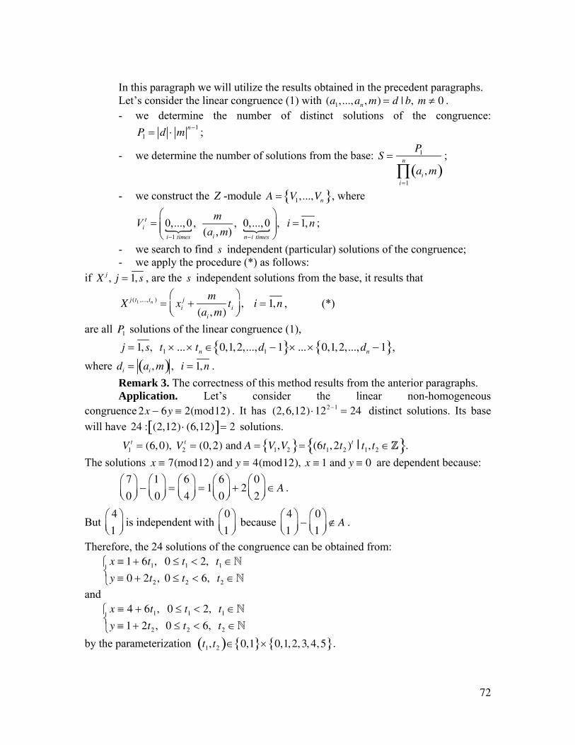
72
In this paragraph we will utilize the results obtained in the precedent paragraphs. Let’s consider the linear congruence (1) with (a1,...,an , m) = d | b, m ≠ 0 .
- we determine the number of distinct solutions of the congruence: P1 = d ⋅ m
n−1 ;
- we determine the number of solutions from the base: S =P1
ai , m( )i=1
n
∏;
- we construct the Z -module A = V1,...,Vn{ }, where
1
0,..., 0 , , 0,..., 0 , 1,( , )
ti
ii times n i times
mV i na m− −
⎛ ⎞= =⎜ ⎟⎜ ⎟
⎝ ⎠;
- we search to find s independent (particular) solutions of the congruence; - we apply the procedure (*) as follows:
if X j , j = 1, s , are the s independent solutions from the base, it results that
X j (t1 ,...,tn ) = xij +
m
(ai ,m)ti
⎛⎝⎜
⎞⎠⎟
, i = 1,n , (*)
are all P1 solutions of the linear congruence (1), j = 1, s, t1 × ...× tn ∈ 0,1,2,...,d1 − 1{ }× ...× 0,1,2,...,dn − 1{ },
where di = ai , m( ) , i = 1,n . Remark 3. The correctness of this method results from the anterior paragraphs. Application. Let’s consider the linear non-homogeneous congruence 2x − 6y ≡ 2(mod12) . It has (2,6,12) ⋅122−1 = 24 distinct solutions. Its base will have 24 : (2,12) ⋅ (6,12)[ ]= 2 solutions.
V1t = (6,0), V2
t = (0,2) and A = V1,V2{ }= (6t1,2t2 )t | t1, t2 ∈Z{ }. The solutions x ≡ 7(mod12) and y ≡ 4(mod12), x ≡ 1 and y ≡ 0 are dependent because:
7
0
⎛⎝⎜
⎞⎠⎟
−1
0
⎛⎝⎜
⎞⎠⎟
=6
4
⎛⎝⎜
⎞⎠⎟
= 16
0
⎛⎝⎜
⎞⎠⎟
+ 20
2
⎛⎝⎜
⎞⎠⎟
∈A .
But 4
1
⎛⎝⎜
⎞⎠⎟
is independent with 0
1
⎛⎝⎜
⎞⎠⎟
because 4
1
⎛⎝⎜
⎞⎠⎟
−0
1
⎛⎝⎜
⎞⎠⎟
∉A .
Therefore, the 24 solutions of the congruence can be obtained from:
x ≡ 1 + 6t1, 0 ≤ t1 < 2, t1 ∈Ny ≡ 0 + 2t2 , 0 ≤ t2 < 6, t2 ∈N
⎧⎨⎩
and
x ≡ 4 + 6t1, 0 ≤ t1 < 2, t1 ∈Ny ≡ 1 + 2t2 , 0 ≤ t2 < 6, t2 ∈N
⎧⎨⎩
by the parameterization t1, t2( )∈ 0,1{ }× 0,1,2, 3, 4,5{ }.
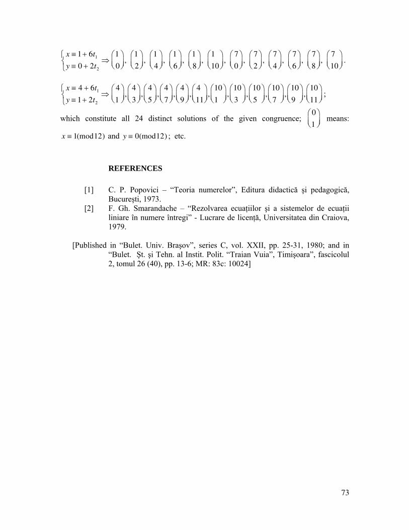
73
x ≡ 1 + 6t1
y ≡ 0 + 2t2
⎧⎨⎩
⇒1
0
⎛⎝⎜
⎞⎠⎟
, 1
2
⎛⎝⎜
⎞⎠⎟
, 1
4
⎛⎝⎜
⎞⎠⎟
, 1
6
⎛⎝⎜
⎞⎠⎟
, 1
8
⎛⎝⎜
⎞⎠⎟
, 1
10
⎛⎝⎜
⎞⎠⎟
, 7
0
⎛⎝⎜
⎞⎠⎟
, 7
2
⎛⎝⎜
⎞⎠⎟
, 7
4
⎛⎝⎜
⎞⎠⎟
, 7
6
⎛⎝⎜
⎞⎠⎟
, 7
8
⎛⎝⎜
⎞⎠⎟
, 7
10
⎛⎝⎜
⎞⎠⎟
.
x ≡ 4 + 6t1
y ≡ 1 + 2t2
⎧⎨⎩
⇒4
1
⎛⎝⎜
⎞⎠⎟
,4
3
⎛⎝⎜
⎞⎠⎟
,4
5
⎛⎝⎜
⎞⎠⎟
,4
7
⎛⎝⎜
⎞⎠⎟
,4
9
⎛⎝⎜
⎞⎠⎟
,4
11
⎛⎝⎜
⎞⎠⎟
,10
1
⎛⎝⎜
⎞⎠⎟
,10
3
⎛⎝⎜
⎞⎠⎟
,10
5
⎛⎝⎜
⎞⎠⎟
,10
7
⎛⎝⎜
⎞⎠⎟
,10
9
⎛⎝⎜
⎞⎠⎟
,10
11
⎛⎝⎜
⎞⎠⎟
;
which constitute all 24 distinct solutions of the given congruence; 0
1
⎛⎝⎜
⎞⎠⎟
means:
x ≡ 1(mod12) and y ≡ 0(mod12) ; etc.
REFERENCES
[1] C. P. Popovici – “Teoria numerelor”, Editura didactică şi pedagogică,
Bucureşti, 1973. [2] F. Gh. Smarandache – “Rezolvarea ecuaţiilor şi a sistemelor de ecuaţii
liniare în numere întregi” - Lucrare de licenţă, Universitatea din Craiova, 1979.
[Published in “Bulet. Univ. Braşov”, series C, vol. XXII, pp. 25-31, 1980; and in
“Bulet. Şt. şi Tehn. al Instit. Polit. “Traian Vuia”, Timişoara”, fascicolul 2, tomul 26 (40), pp. 13-6; MR: 83c: 10024]
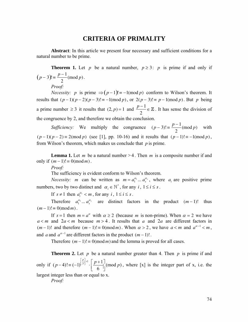
74
CRITERIA OF PRIMALITY
Abstract: In this article we present four necessary and sufficient conditions for a natural number to be prime. Theorem 1. Let p be a natural number, p ≥ 3 : p is prime if and only if
p − 3( )! ≡p − 1
2(mod p) .
Proof: Necessity: p is prime ⇒ p − 1( )! ≡ −1(mod p) conform to Wilson’s theorem. It results that (p − 1)(p − 2)(p − 3)! ≡ −1(mod p) , or 2(p − 3)! ≡ p − 1(mod p) . But p being
a prime number ≥ 3 it results that (2, p) = 1 and p − 1
2∈Z . It has sense the division of
the congruence by 2, and therefore we obtain the conclusion.
Sufficiency: We multiply the congruence ( p − 3)! ≡p − 1
2(mod p) with
( p − 1)( p − 2) ≡ 2(mod p) (see [1], pp. 10-16) and it results that (p − 1)! ≡ −1(mod p) , from Wilson’s theorem, which makes us conclude that p is prime. Lemma 1. Let m be a natural number > 4 . Then m is a composite number if and only if (m − 1)! ≡ 0(mod m) . Proof: The sufficiency is evident conform to Wilson’s theorem. Necessity: m can be written as m = a1
α1 ... asα s , where ai are positive prime
numbers, two by two distinct and α i ∈N* , for any i , 1 ≤ i ≤ s . If 1s ≠ then ai
αi < m , for any i , 1 ≤ i ≤ s . Therefore a1
α1 ... asα s are distinct factors in the product (m − 1)! thus
(m − 1)! ≡ 0(mod m) . If 1s = then m = aα with α ≥ 2 (because m is non-prime). When α = 2 we have a < m and 2a < m because m > 4 . It results that a and 2a are different factors in (m − 1)! and therefore (m − 1)! ≡ 0(mod m) . When α > 2 , we have a < m and aα −1 < m , and a and aα −1 are different factors in the product (m − 1)! . Therefore (m − 1)! ≡ 0(mod m) and the lemma is proved for all cases. Theorem 2. Let p be a natural number greater than 4. Then p is prime if and
only if 1
3 1( 4)! ( 1) (mod )6
p pp p⎡ ⎤+⎢ ⎥⎣ ⎦ +⎡ ⎤− ≡ − ⋅ ⎢ ⎥⎣ ⎦
, where [x] is the integer part of x, i.e. the
largest integer less than or equal to x. Proof:
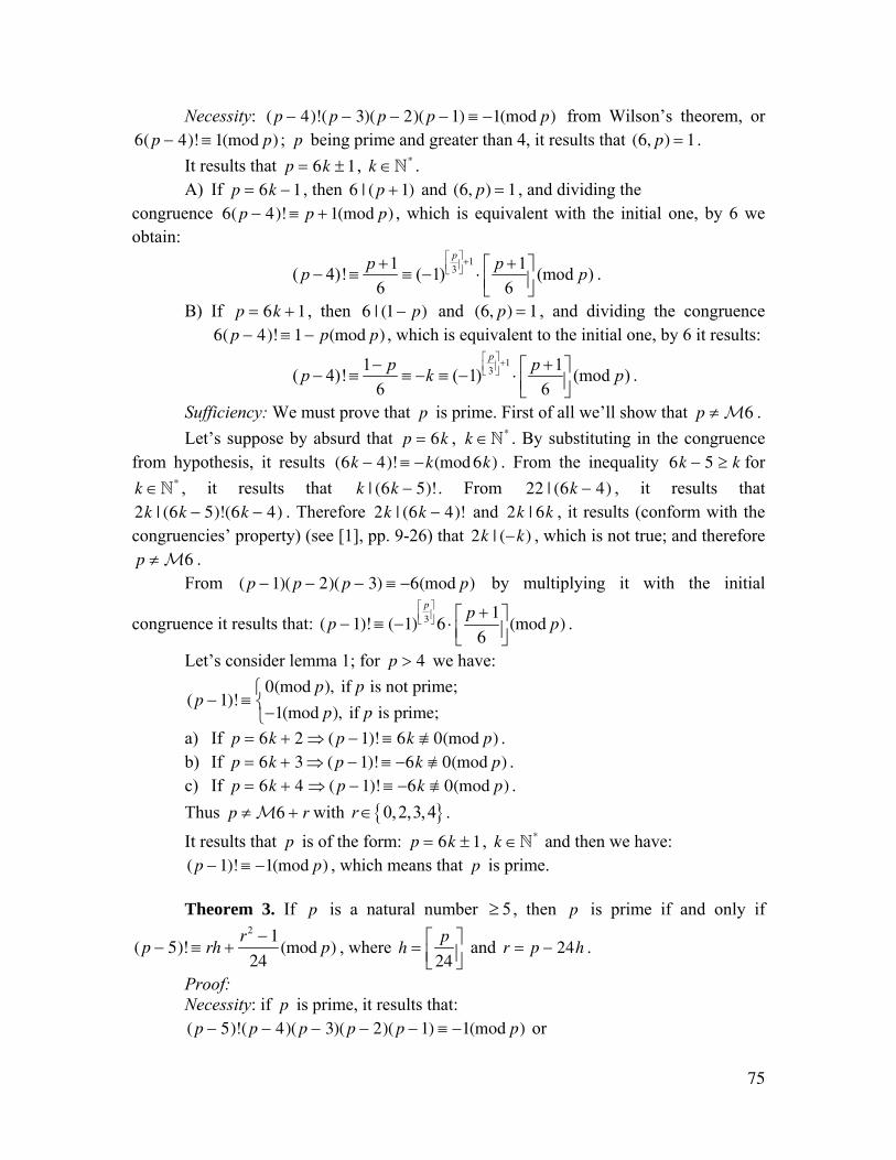
75
Necessity: ( p − 4)!(p − 3)(p − 2)( p − 1) ≡ −1(mod p) from Wilson’s theorem, or 6( p − 4)! ≡ 1(mod p) ; p being prime and greater than 4, it results that (6, p) = 1 . It results that p = 6k ± 1, k ∈N* .
A) If p = 6k − 1 , then 6 | (p + 1) and (6, p) = 1 , and dividing the congruence 6( p − 4)! ≡ p + 1(mod p) , which is equivalent with the initial one, by 6 we obtain:
1
31 1( 4)! ( 1) (mod )6 6
pp pp p⎡ ⎤+⎢ ⎥⎣ ⎦+ +⎡ ⎤− ≡ ≡ − ⋅ ⎢ ⎥⎣ ⎦
.
B) If p = 6k + 1 , then 6 | (1 − p) and (6, p) = 1 , and dividing the congruence 6( p − 4)! ≡ 1 − p(mod p) , which is equivalent to the initial one, by 6 it results:
131 1( 4)! ( 1) (mod )
6 6
pp pp k p⎡ ⎤+⎢ ⎥⎣ ⎦− +⎡ ⎤− ≡ ≡ − ≡ − ⋅ ⎢ ⎥⎣ ⎦
.
Sufficiency: We must prove that p is prime. First of all we’ll show that p ≠ M6 . Let’s suppose by absurd that p = 6k , k ∈N* . By substituting in the congruence from hypothesis, it results (6k − 4)! ≡ −k(mod 6k) . From the inequality 6k − 5 ≥ k for
k ∈N* , it results that k | (6k − 5)!. From 22 | (6k − 4) , it results that 2k | (6k − 5)!(6k − 4) . Therefore 2k | (6k − 4)! and 2k | 6k , it results (conform with the congruencies’ property) (see [1], pp. 9-26) that 2k | (−k) , which is not true; and therefore
p ≠ M6 . From ( p − 1)( p − 2)( p − 3) ≡ −6(mod p) by multiplying it with the initial
congruence it results that: (p − 1)! ≡ (−1)p
3⎡⎣⎢
⎤⎦⎥ 6 ⋅
p + 1
6⎡⎣⎢
⎤⎦⎥(mod p) .
Let’s consider lemma 1; for p > 4 we have:
(p − 1)! ≡0(mod p), if p is not prime;
−1(mod p), if p is prime;
⎧⎨⎩
a) If p = 6k + 2 ⇒ (p − 1)! ≡ 6k /≡ 0(mod p) . b) If p = 6k + 3 ⇒ (p − 1)! ≡ −6k /≡ 0(mod p) . c) If p = 6k + 4 ⇒ ( p − 1)! ≡ −6k /≡ 0(mod p) . Thus p ≠ M6 + r with { }0,2,3,4r ∈ .
It results that p is of the form: p = 6k ± 1, k ∈N* and then we have: (p − 1)! ≡ −1(mod p) , which means that p is prime.
Theorem 3. If p is a natural number 5≥ , then p is prime if and only if
(p − 5)! ≡ rh +r2 − 1
24(mod p) , where h =
p
24⎡⎣⎢
⎤⎦⎥
and r = p − 24h .
Proof: Necessity: if p is prime, it results that: ( p − 5)!( p − 4)( p − 3)( p − 2)( p − 1) ≡ −1(mod p) or
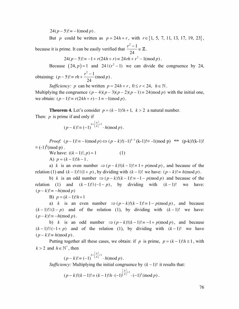
76
24(p − 5)! ≡ −1(mod p) . But p could be written as p = 24h + r , with { }1, 5, 7, 11, 13, 17, 19, 23r ∈ ,
because it is prime. It can be easily verified that r2 − 1
24∈Z .
24(p − 5)! ≡ −1 + r(24h + r) ≡ 24rh + r2 − 1(mod p) . Because ( )24, 1p = and 24 | (r2 − 1) we can divide the congruence by 24,
obtaining: (p − 5)! ≡ rh +r2 − 1
24(mod p) .
Sufficiency: p can be written p = 24h + r , 0 ≤ r < 24, h ∈N . Multiplying the congruence ( p − 4)( p − 3)( p − 2)( p − 1) ≡ 24(mod p) with the initial one, we obtain: ( p − 1)! ≡ r(24h + r) − 1 ≡ −1(mod p) . Theorem 4. Let’s consider p = (k − 1)!h + 1, k > 2 a natural number. Then: p is prime if and only if
( p − k)! ≡ (−1)h+
p
h⎡⎣⎢
⎤⎦⎥+1
⋅ h(mod p) .
Proof: (p − 1)! ≡ −1(mod p) ⇔ (p − k)!(−1)k −1 (k-1)!≡ -1(mod p) ] (p-k)!(k-1)! ≡ (-1)k(mod p) . We have: ((k − 1)!, p) = 1 (1) A) p = (k − 1)!h − 1 . a) k is an even number ⇒ (p − k)!(k − 1)! ≡ 1 + p(mod p) , and because of the relation (1) and (k − 1)! | (1 + p) , by dividing with (k − 1)! we have: ( p − k)! ≡ h(mod p) . b) k is an odd number ⇒ ( p − k)!(k − 1)! ≡ −1 − p(mod p) and because of the relation (1) and (k − 1)! | (−1 − p) , by dividing with (k − 1)! we have: ( p − k)! ≡ −h(mod p) B) ( 1)! 1p k h= − + a) k is an even number ⇒ (p − k)!(k − 1)! ≡ 1 − p(mod p) , and because (k − 1)! | (1 − p) and of the relation (1), by dividing with (k − 1)! we have: ( )! (mod )p k h p− ≡ − . b) k is an odd number ⇒ ( p − k)!(k − 1)! ≡ −1 + p(mod p) , and because (k − 1)! | (−1 + p) and of the relation (1), by dividing with (k − 1)! we have ( p − k)! ≡ h(mod p) . Putting together all these cases, we obtain: if p is prime, p = (k − 1)!h ± 1 , with k > 2 and h ∈N* , then
( p − k)! ≡ (−1)h+
p
h⎡⎣⎢
⎤⎦⎥+1
⋅ h(mod p) . Sufficiency: Multiplying the initial congruence by (k − 1)! it results that:
( p − k)!(k − 1)! ≡ (k − 1)!h ⋅ (−1)p
h⎡⎣⎢
⎤⎦⎥+1
⋅ (−1)k (mod p) .
77
Analyzing separately each of these cases:
A) p = (k − 1)!h − 1 and B) p = (k − 1)!h + 1 , we obtain for both, the congruence:
(p − k)!(k − 1)! ≡ (−1)k (mod p) which is equivalent (as we showed it at the beginning of this proof) with (p − 1)! ≡ −1(mod p) and it results that p is prime. REFERENCE:
[1] Constantin P. Popovici, “Teoria numerelor”, Editura Didactică şi Pedagogică, Bucharest, 1973.
[Published in “Gazeta Matematică”, Bucharest, Year XXXVI, No. 2, pp. 49-52,
February 1981]
78
INTEGER ALGORITHMS TO SOLVE DIOPHANTINE
LINEAR EQUATIONS AND SYSTEMS Abstract: Two algorithms for solving Diophantine linear equations and five algorithms for solving Diophantine linear systems, together with many examples, are presented in this paper. Keywords: Diophantine equations, Diophantine systems, particular integer solutions, general integer solutions
Contents: Introduction Properties of Integer Solutions of Linear Equations An Integer Number Algorithm to Solve Linear Equations Another Integer Number Algorithm to Solve Linear Equations (Using Congruences) Properties of Integer Number Solutions of Linear Systems Five Integer Number Algorithms to Solve Linear Systems
79
Introduction: The present work includes some of the author’s original researches on the integer solutions of equations and linear systems:
1. The notion of “general integer solution” of a linear equation with two unknowns is extended to linear equations with n unknowns and then, to linear systems.
2. The properties of the general integer solution are determined (both of a linear equation and of a linear system).
3. Seven original integer algorithms (two for linear equations and five for linear systems) are presented. The algorithms are carefully demonstrated and an example for each of them is presented. These algorithms can be easily introduced into computer.
80
INTEGER SOLUTIONS OF LINEAR EQUATIONS
Definitions and properties of the integer solutions of linear equations. Consider the following linear equation:
(1) aixii=1
n
∑ = b ,
with all ai ≠ 0 and b in Z . Again, let h ∈N , and fi :Zh → Z , i = 1,n . (1,n means: all integers from 1 to n ). Definition 1. xi = xi
0 , i = 1,n , is a particular integer solution of equation (1), if all xi0 ∈Z and
ai xi0
i=1
n
∑ = b .
Definition 2. xi = fi (k1,..., kh ) , i = 1,n , is the general integer solution of equation (1) if:
a)
ai fi (k1,..., kh )i=1
n
∑ = b; ∀(k1,...,kh ) ∈Zh ,
b) For any particular integer solution of equation (1), xi = xi0 , i = 1,n , there exist
0 01( ,..., ) h
hk k ∈Z such that xi0 = fi (k1
0 ,..., kh0 ) for all i = 1,n {i. e. any particular integer
solution can be extracted from the general integer solution by parameterization}. We will further see that the general integer solution can be expressed by linear functions.
For 1 ≤ i ≤ n we consider the functions fi = cijk j + dij =1
h
∑ with all cij , di ∈Z .
Definition 3.
A = (cij )i, j is the matrix associated with the general solution of equation (1).
Definition 4. The integers k1,..., ks , 1 ≤ s ≤ h are independent if all the corresponding column vectors of matrix A are linearly independent. Definition 5. An integer solution is s -times undetermined if the maximal number of independent parameters is s . Theorem 1. The general integer solution of equation (1) is n − 1( )-times undetermined.
81
Proof: We suppose that the particular integer solution is of the form:
(2) xi = uiePe + vie=1
r
∑ , i = 1,n , with all uie, vi ∈Z ,
Pe are parameters of Z , while a ≤ r < n − 1 . Let (x1
0 ,..., xn0 ) be a general integer solution of equation (1) (we are not interested in
the case when the equation does not have an integer solution). The solution:
xj = ank j + x j0 , j = 1,n − 1
xn = − ajk j − xn0
j =1
n−1
∑⎛
⎝⎜⎞
⎠⎟
⎧
⎨⎪
⎩⎪
is undetermined n − 1( )-times (it can be easily checked that the order of the associated matrix is n − 1 ). Hence, there are n − 1 undetermined solutions. Let’s consider, in the general case, a solution be undetermined n − 1( )-times:
xi = cijk j + dij =1
n−1
∑ , i = 1,n with all cij , di ∈Z .
Consider the case when b = 0 . Then
aixi = 0i=1
n
∑ .
It follows:
ai xi = aii=1
n
∑ cijk j + dij =1
n−1
∑⎛
⎝⎜⎞
⎠⎟= ai
i=1
n
∑ cijk j +j =1
n−1
∑ aii=1
n
∑ di = 0i=1
n
∑ .
For k j = 0 , j = 1,n − 1 it follows that aii=1
n
∑ di = 0 .
For kj0= 1 and k j = 0, j ≠ j0 , it follows that ai
i=1
n
∑ cij0= 0 .
Let’s consider the homogenous linear system of n equations with n unknowns:
xi
i=1
n
∑ cij = 0, j = 1,n − 1
xii=1
n
∑ di = 0
⎧
⎨⎪⎪
⎩⎪⎪
which, obviously, has the solution xi = ai , i = 1,n different from the trivial one. Hence
the determinant of the system is zero, i.e., the vectors cj = c1 j ,...,cnj( )t, j = 1,n − 1 ,
D = d1,...,dn( )t are linearly dependent.
82
But the solution being n − 1( )-times undetermined it shows that cj , j = 1,n − 1 are
linearly independent. Then c1,...,cn−1( ) determines a free sub-module Z of order n − 1 in
Zn of solutions for the given equation. Let’s see what can we obtain from (2). We have:
0 = aii=1
n
∑ xi = aii=1
n
∑ uiePe + vie=1
r
∑⎛⎝⎜
⎞⎠⎟
.
As above, we obtain:
aii =1
n
∑ vi = 0 and aiuie0= 0
e=1
r
∑
similarly, the vectors Uh = u1h ,...,unh( ) are linearly independent, h = 1,r , Uh , h = 1,r are V = v1,...,vn( ) particular integer solutions of the homogenous linear equation. Sub-case (a1) U,h = 1,r are linearly dependent. This gives { }1,..., rU U = the free sub-module of
order r in Zn of solutions of the equation. Hence, there are solutions from { }1 1,..., nV V −
which are not from { }1,..., rU U ; this contradicts the fact that (2) is the general integer solution. Sub-case (a2) Uh , h = 1,r, V are linearly independent. Then { }1,..., rU U V+ is a linear variety
of the dimension { }1 11 dim ,..., nn V V −< − = and the conclusion can be similarly drawn.
Consider the case when b ≠ 0 . So, aii=1
n
∑ xi = b .
Then:
ai cijk j + di
j =1
n−1
∑⎛
⎝⎜⎞
⎠⎟= aicij
i=1
n
∑⎛⎝⎜
⎞⎠⎟j =1
n−1
∑ kj + aii=1
n
∑ dii=1
n
∑ = b; ∀(k1,...,kn−1) ∈Zn−1 .
As in the previous case, we obtain aii=1
n
∑ di = b and aii=1
n
∑ cij = 0, ∀ j = 1,n − 1.
The vectors ( ),...,t
j ij njc c c= , j = 1,n − 1 , are linearly independent because the solution is
undetermined n − 1( )-times.
Conversely, if c1,...,cn−1, D (where D = d1,...,dn( )t ) were linearly dependent, it
would mean that D = sjcjj =1
n−1
∑ with all s j scalar; it would also mean that
b = aii=1
n
∑ di = aii=1
n
∑ s jcijj =1
n−1
∑⎛
⎝⎜⎞
⎠⎟= s j ai
i=1
n
∑ cij
⎛⎝⎜
⎞⎠⎟j =1
n−1
∑ = 0 .
This is impossible. (3) Then { }1 1,..., nc c D− + is a linear variety.
83
Let us see what we can obtain from (2). We have:
b = aii=1
n
∑ xi = aii=1
n
∑ uiePe + vie=1
r
∑⎛⎝⎜
⎞⎠⎟
= aii=1
n
∑ uie
⎛⎝⎜
⎞⎠⎟
Pe + aii=1
n
∑ vie=1
r
∑
and, similarly: aii =1
n
∑ vi = b and aii=1
n
∑ uie = 0, ∀ e = 1,r , respectively. The vectors
( )1 ,..., te e neU u u= , e = 1,r are linearly independent because the solution is undetermined
r -times. A procedure like that applied in (3) shows that U1,...,Ur , V are linearly
independent, where ( )1,...,t
nV v v= . Then { }1,..., rU U V+ = a linear variety = free sub-
module of order r < n − 1. That is, we can find vectors from { }1 1,..., nc c D− + which are
not from { }1,..., rU U V+ , contradicting the “general” characteristic of the integer number solution. Hence, the general integer solution is undetermined n − 1( )-times. Theorem 2. The general integer solution of the homogeneous linear equation
aixii=1
n
∑ = 0 (all { }\ 0ia ∈Z ) can be written under the form:
(4) xi = cijk j , j =1
n−1
∑ i = 1,n
(with d1 = ... = dn = 0 ). Definition 6. This is called the standard form of the general integer solution of a homogeneous linear equation. Proof:
We consider the general integer solution under the form:
xi = cijPj + di , j =1
n−1
∑ i = 1,n
with not all di = 0 . We’ll show that it can be written under the form (4). The homogeneous equation has the trivial solution xi = 0, i = 1,n . There is
p10 ,..., pn−1
0( )∈Zn−1 such that cij pj0 + di = 0, ∀
j =1
n−1
∑ i = 1,n .
Substituting: Pj = k j + pj , j = 1,n − 1 in the form shown at the beginning of the demonstration, we will obtain form (4). We have to mention that the substitution does not diminish the degree of generality as Pj ∈Z ⇔ k j ∈Z because j = 1,n − 1 . Theorem 3. The general integer solution of a non-homogeneous linear equation is equal to the general integer solution of its associated homogeneous linear equation plus any particular integer solution of the non-homogeneous linear equation. Proof:
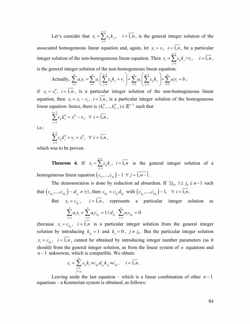
84
Let’s consider that 1
1
, 1,n
i ij jj
x c k i n−
=
= =∑ , is the general integer solution of the
associated homogeneous linear equation and, again, let xi = vi , i = 1,n , be a particular
integer solution of the non-homogeneous linear equation. Then 1
1
+ , 1,n
i ij j ij
x c k v i n−
=
= =∑ ,
is the general integer solution of the non-homogeneous linear equation.
Actually, 1 1
1 1 1 1 1 1
n n n n n n
i i i ij j i i ij j i ii i j i j i
a x a c k v a c k a v b− −
= = = = = =
⎛ ⎞ ⎛ ⎞= + = + =⎜ ⎟ ⎜ ⎟
⎝ ⎠ ⎝ ⎠∑ ∑ ∑ ∑ ∑ ∑ ;
if xi = xi0 , i = 1,n , is a particular integer solution of the non-homogeneous linear
equation, then xi = xi − vi , i = 1,n , is a particular integer solution of the homogeneous linear equation: hence, there is (k1
0 ,..., kn−10 ) ∈Zn−1 such that
cijj =1
n−1
∑ kj0 = x
i
0 − vi , ∀ i = 1,n ,
i.e.:
cijj =1
n−1
∑ kj0 + vi = x
i
0 , ∀ i = 1,n ,
which was to be proven.
Theorem 4. If 1
1
, 1,n
i ij jj
x c k i n−
=
= =∑ is the general integer solution of a
homogeneous linear equation ( ),..., 1ij njc c ∼ 1, 1j n∀ = − .
The demonstration is done by reduction ad absurdum. If 0 0, 1 1j j n∃ ≤ ≤ − such
that ( )0 0 0,..., 1ij nj jc c d ≠ ±∼ , then cij0
= cij0
' dij0 with ( )0 0
' ',..., 1, 1,ij njc c i n∀ =∼ .
But xi = cij0
' , i = 1,n , represents a particular integer solution as
aii=1
n
∑ xi = aii=1
n
∑ cij0
' = 1 / dj0⋅ aicij0
= 0i=1
n
∑
(because xi = cij0, i = 1,n is a particular integer solution from the general integer
solution by introducing kj0= 1 and k j = 0 , j ≠ j0 . But the particular integer solution
xi = cij0
' , i = 1,n , cannot be obtained by introducing integer number parameters (as it should) from the general integer solution, as from the linear system of n equations and n − 1 unknowns, which is compatible. We obtain:
xi = cijk jj =1j ≠ j0
n
∑ +cij0
' dj0kj0
=cij0
' , i = 1,n .
Leaving aside the last equation – which is a linear combination of other n − 1 equations – a Kramerian system is obtained, as follows:
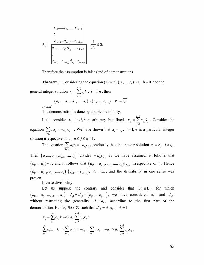
85
0
0
0
00 0
0 0
'11 1, 1
'1,1 1 1 1
'11 1, 1
'1,1 1 1 1
...... .......
:... ... 1
....... ......
:... ...
ij n
n n j n nj
jij j n
n n j j n n
c c c
c c ck
dc c d c
c c d c
−
− − − −
−
− − − −
= = ∉Z
Therefore the assumption is false (end of demonstration).
Theorem 5. Considering the equation (1) with ( )1,..., 1, 0na a b =∼ and the
general integer solution xi = cijk jj =1
n−1
∑ , i = 1,n , then
( ) ( )1 1 1 1 1,..., , ,..., ,..., , 1,i i n i ina a a a c c i n− + − ∀ =∼ . Proof: The demonstration is done by double divisibility.
Let’s consider i0 , 1 ≤ i0 ≤ n arbitrary but fixed. xi0= ci0 jk j
j =1
n−1
∑ . Consider the
equation ai xi = −i≠ i0
∑ ai0xi0
. We have shown that xi = cij , i = 1,n is a particular integer
solution irrespective of j, a ≤ j ≤ n − 1 . The equation ai xi = −
i≠ i0
∑ ai0ci0 j obviously, has the integer solution xi = cij , i ≠ i0 .
Then ( )0 01 1 1,..., , ,...,i i na a a a− + divides − ai0ci0 j as we have assumed, it follows that
( )1,..., 1na a ∼ , and it follows that ( )0 0 01 1 1,..., , ,..., |i i n i ja a a a c− + irrespective of j . Hence
( ) ( )0 0 0 01 1 1 1 1,..., , ,..., | ,..., , 1,i i n i i na a a a c c i n− + − ∀ = , and the divisibility in one sense was
proven. Inverse divisibility: Let us suppose the contrary and consider that ∃i1 ∈1,n for which
( ) ( )1 1 1 1 1 11 1 1 1 2 1 1,..., , ,..., ,...,i i n i i i i na a a a d d c c− + −≠∼ ∼ ; we have considered di11 and di1 2 without restricting the generality. di11 | di1 2 according to the first part of the
demonstration. Hence, ∃d ∈Z such that 1 12 1, 1i id d d d= ⋅ ≠ .
xi1= ci1 jk j
j =1
n−1
∑ =d ⋅ di11 ci1 j' kj
j =1
n−1
∑ ;
ai xii=1
n
∑ = 0 ⇒ ai xii≠ i1
n
∑ = −ai1xi1
ai xi = −ai1d ⋅ di11
i ≠ i1
∑ ci1 j' k j
j =1
n−1
∑ ,
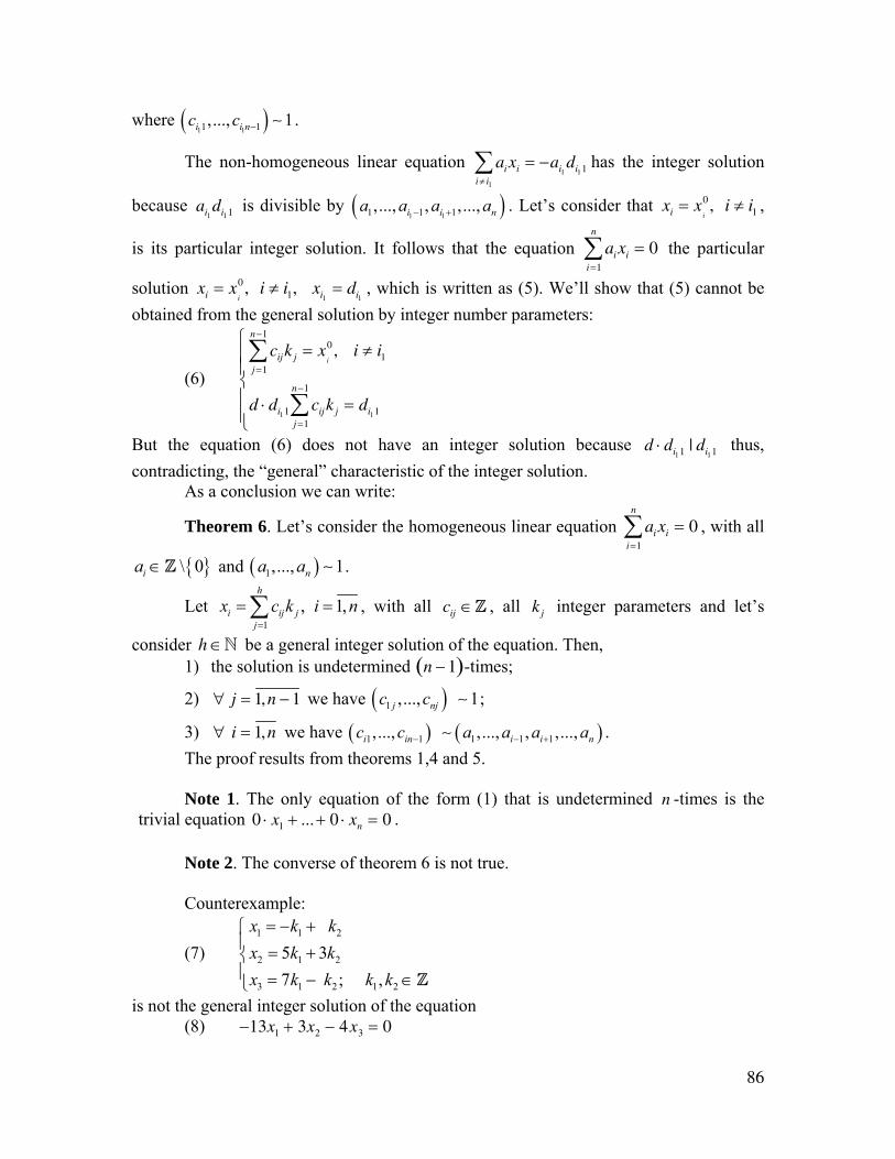
86
where ( )1 11 1,..., 1i i nc c − ∼ .
The non-homogeneous linear equation ai xi = −ai1di11
i ≠ i1
∑ has the integer solution
because ai1di11 is divisible by ( )1 11 1 1,..., , ,...,i i na a a a− + . Let’s consider that xi = x
i
0 , i ≠ i1 ,
is its particular integer solution. It follows that the equation aii=1
n
∑ xi = 0 the particular
solution xi = xi
0 , i ≠ i1, xi1= di1
, which is written as (5). We’ll show that (5) cannot be obtained from the general solution by integer number parameters:
(6) cij
j =1
n−1
∑ k j = xi
0 , i ≠ i1
d ⋅ di11 cijj =1
n−1
∑ k j = di11
⎧
⎨⎪⎪
⎩⎪⎪
But the equation (6) does not have an integer solution because d ⋅ di11 | di11 thus, contradicting, the “general” characteristic of the integer solution. As a conclusion we can write:
Theorem 6. Let’s consider the homogeneous linear equation aii=1
n
∑ xi = 0 , with all
{ }\ 0ia ∈Z and ( )1,..., 1na a ∼ .
Let 1
, 1,h
i ij jj
x c k i n=
= =∑ , with all cij ∈Z , all kj integer parameters and let’s
consider h ∈N be a general integer solution of the equation. Then, 1) the solution is undetermined n − 1( )-times;
2) ∀ j = 1,n − 1 we have ( )1 ,..., 1j njc c ∼ ;
3) ∀ i = 1,n we have ( ) ( )1 1 1 1 1,..., ,..., , ,...,i in i i nc c a a a a− − +∼ . The proof results from theorems 1,4 and 5. Note 1. The only equation of the form (1) that is undetermined n -times is the
trivial equation 0 ⋅ x1 + ...+ 0 ⋅ xn = 0 .
Note 2. The converse of theorem 6 is not true.
Counterexample:
(7) 1 1 2
2 1 2
3 1 2 1 2
5 37 ; ,
x k kx k kx k k k k
= − +⎧⎪ = +⎨⎪ = − ∈⎩ Z
is not the general integer solution of the equation (8) −13x1 + 3x2 − 4x3 = 0
87
although the solution (7) verifies the points 1), 2) and 3) of theorem 6. (1, 7, 2) is the particular integer solution of (8) but cannot be obtained by introducing integer number parameters in (7) because from
1 2
1 2
1 2
15 3 77 = 2
k kk kk k
− + =⎧⎪ + =⎨⎪ −⎩
it follows that 12
k = ∉Z and 32
k = ∉Z (unique roots).
REFERENCE
[1] Smarandache, Florentin – Whole number solution of linear equations and systems – diploma thesis work, 1979, University of Craiova (under the supervision of Assoc. Prof. Dr. Alexandru Dincă)
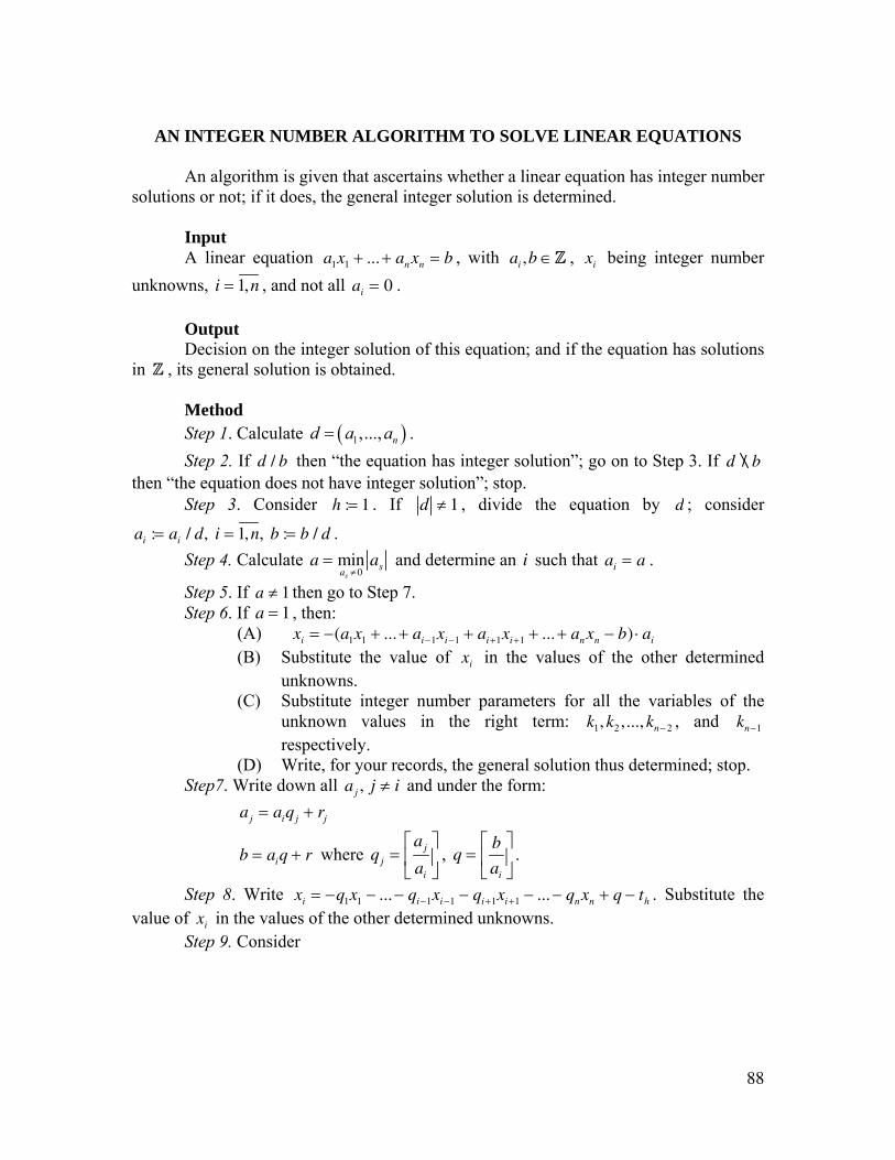
88
AN INTEGER NUMBER ALGORITHM TO SOLVE LINEAR EQUATIONS
An algorithm is given that ascertains whether a linear equation has integer number solutions or not; if it does, the general integer solution is determined. Input A linear equation a1x1 + ... + anxn = b , with ai ,b ∈Z , xi being integer number unknowns, i = 1,n , and not all ai = 0 . Output Decision on the integer solution of this equation; and if the equation has solutions in Z , its general solution is obtained. Method Step 1. Calculate ( )1,..., nd a a= . Step 2. If d / b then “the equation has integer solution”; go on to Step 3. If d / b then “the equation does not have integer solution”; stop. Step 3. Consider h := 1 . If d ≠ 1 , divide the equation by d ; consider
ai := ai / d, i = 1,n, b := b / d . Step 4. Calculate a = min
as ≠0as and determine an i such that ai = a .
Step 5. If a ≠ 1 then go to Step 7. Step 6. If a = 1 , then: (A) xi = −(a1x1 + ... + ai −1xi −1 + ai +1xi +1 + ... + anxn − b) ⋅ ai
(B) Substitute the value of xi in the values of the other determined unknowns.
(C) Substitute integer number parameters for all the variables of the unknown values in the right term: k1, k2 ,..., kn− 2 , and kn−1 respectively.
(D) Write, for your records, the general solution thus determined; stop. Step7. Write down all aj , j ≠ i and under the form:
aj = aiqj + rj
b = aiq + r where qj =aj
ai
⎡
⎣⎢
⎤
⎦⎥ , q =
b
ai
⎡
⎣⎢
⎤
⎦⎥ .
Step 8. Write xi = −q1x1 − ...− qi −1xi −1 − qi+1xi +1 − ... − qnxn + q − th . Substitute the value of xi in the values of the other determined unknowns. Step 9. Consider
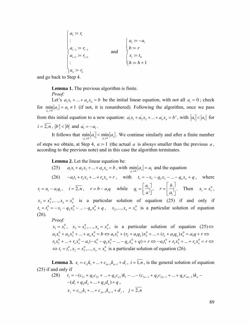
89
a1 := r1:
ai−1 := ri−1
ai+1 := ri+1
:
an := rn
⎧
⎨
⎪⎪⎪
⎩
⎪⎪⎪
and
ai := −ai
b := r
xi := th
h := h + 1
⎧
⎨⎪⎪
⎩⎪⎪
and go back to Step 4. Lemma 1. The previous algorithm is finite. Proof: Let’s a1x1 + ... + anxn = b be the initial linear equation, with not all ai = 0 ; check for min
as ≠0as = a1 ≠ 1 (if not, it is renumbered). Following the algorithm, once we pass
from this initial equation to a new equation: ' ' '1 1 2 2 ... 'n na x a x a x b+ + + = , with '
1 ia a< for
i = 2,n , b ' < b and '1 1a a= − .
It follows that '
'
10min min
sss saa
a a≠≠
< . We continue similarly and after a finite number
of steps we obtain, at Step 4, a := 1 (the actual a is always smaller than the previous a , according to the previous note) and in this case the algorithm terminates. Lemma 2. Let the linear equation be: (25) 1 1 2 2 ... n na x a x a x b+ + + = , with 10
mins
saa a
≠= and the equation
(26) 1 1 2 2 ... n na t r x r x r− + + + = , with t1 = −x1 − q2x2 − ... − qnxn + q , where
ri = ai − aiqi , i = 2,n , r = b − a1q while qi =ai
a⎡⎣⎢
⎤⎦⎥
, 1
bra
⎡ ⎤= ⎢ ⎥
⎣ ⎦. Then x1 = x1
0 ,
x2 = x20 ,…, xn = xn
0 is a particular solution of equation (25) if and only if t1 = t1
0 = −x1 − q2x20 − ... − qnxn
0 + q , x2 ,..., xn = xn0 is a particular solution of equation
(26). Proof:
x1 = x10 , x2 = x2
0 ,…, xn = xn0 , is a particular solution of equation (25) ⇔
a1x10 + a2x2
0 + ... + anxn0 = b ⇔ a1x1
0 + (r2 + a1q2 )x20 + ... + (rn + a1qn )xn
0 = a1q + r ⇔ r2x2
0 + ... + rnxn0 − a1(−x1
0 − q2x20 − ... − qnxn
0 + q) = r ⇔ −a1t10 + r2x2
0 + ... + rnxn0 = r ⇔
0 0 01 1 2 2, ,..., n nt t x x x x⇔ = = = is a particular solution of equation (26).
Lemma 3. 1 1 1 1...i i in n ix c k c k d− −= + + + , i = 1,n , is the general solution of equation (25) if and only if
(28) t1 = −(c11 + q2c21 + ... + qncn1)k1 − ... − (c1n−1 + q2c2n−1 + ... + qncnn−1)kn − 1 2 2( ... )n nd q d q d q− + + + + ,
1 1 1 1 1...j j jn n jx c k c k d− −= + + + , j = 2,n
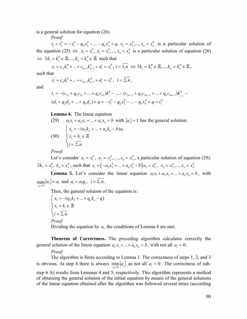
90
is a general solution for equation (26). Proof: t1 = t1
0 = −x10 − q2x2
0 − ... − qnxn0 + q, x2 = x2
0 ,..., xn = xn0 is a particular solution of
the equation (25) ⇔ 0 0 01 1 2 2, ,..., n nx x x x x x= = = is a particular solution of equation (26)
0 01 1 ,..., n nk k k k⇔ ∃ = ∈ = ∈Z Z such that
0 0 01 1 1 1...i i in n i ix c k c k d x− −= + + + = , i = 1,n ⇔ ∃k1 = k1
0 ∈Z,..., kn = kn0 ∈Z ,
such that 0 0 0
1 1 1 1...i i in n i ix c k c k d x− −= + + + = , i = 2,n , and
t1 = −(c11 + q2c21 + ... + qncn1)k1
0 − ... − (c1n−1 + q2c2n−1 + ... + qncnn−1)kn−1
0 −
(d1 + q2d2 + ... + qndn ) + q = −x10 − q2x2
0 − ... − qnxn0 + q = t1
0
Lemma 4. The linear equation (29) 1 1 2 2 ... n na x a x a x b+ + + = with a1 = 1 has the general solution:
(30)
x1 = −(a2k2 + ...+ ankn − b)a1
xi = ki ∈Zi = 2,n
⎧
⎨⎪
⎩⎪
Proof: Let’s consider x1 = x1
0 , x2 = x20 ,…, xn = xn
0 , a particular solution of equation (29). 0 0
2 2 , n nk x k x∃ = = , such that ( )0 0 0 0 01 2 2 1 1 2 2... , ,...,n n n nx a x a x b a x x x x x= − + + − = = = .
Lemma 5. Let’s consider the linear equation 1 1 2 2 ... n na x a x a x b+ + + = , with
10
mins
sa
a a≠
= and 1 , 2,i ia a q i n= = .
Then, the general solution of the equation is:
1 2 2( ... )
2,
n n
i i
x q k q k qx k
i n
⎧ = − + + −⎪
= ∈⎨⎪ =⎩
Z
Proof: Dividing the equation by a1 the conditions of Lemma 4 are met. Theorem of Correctness. The preceding algorithm calculates correctly the general solution of the linear equation 1 1 ... n na x a x b+ + = , with not all ai = 0 . Proof: The algorithm is finite according to Lemma 1. The correctness of steps 1, 2, and 3 is obvious. At step 4 there is always
0min
ssa
a≠
as not all ai = 0 . The correctness of sub-
step 6 A) results from Lemmas 4 and 5, respectively. This algorithm represents a method of obtaining the general solution of the initial equation by means of the general solutions of the linear equation obtained after the algorithm was followed several times (according
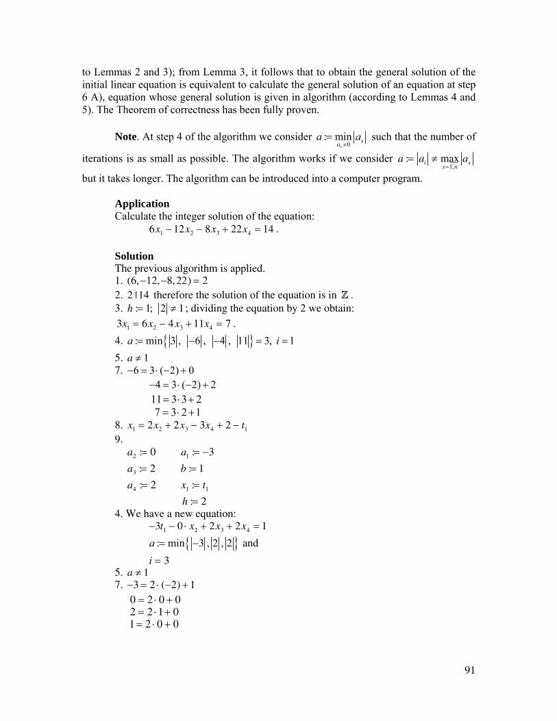
91
to Lemmas 2 and 3); from Lemma 3, it follows that to obtain the general solution of the initial linear equation is equivalent to calculate the general solution of an equation at step 6 A), equation whose general solution is given in algorithm (according to Lemmas 4 and 5). The Theorem of correctness has been fully proven. Note. At step 4 of the algorithm we consider
0: min
ssa
a a≠
= such that the number of
iterations is as small as possible. The algorithm works if we consider a := ai ≠ maxs=1,n
as
but it takes longer. The algorithm can be introduced into a computer program. Application Calculate the integer solution of the equation:
6x1 − 12x2 − 8x3 + 22x4 = 14 . Solution
The previous algorithm is applied. 1. (6,−12,−8,22) = 2 2. 2 |14 therefore the solution of the equation is in Z .
3. h := 1; 2 ≠ 1; dividing the equation by 2 we obtain:
3x1 = 6x2 − 4x3 + 11x4 = 7 .
4. { }: min 3 , 6 , 4 , 11 3, 1a i= − − = =
5. a ≠ 1 7. 6 3 ( 2) 0− = ⋅ − + 4 3 ( 2) 2− = ⋅ − + 11 3 3 2= ⋅ + 7 3 2 1= ⋅ + 8. x1 = 2x2 + 2x3 − 3x4 + 2 − t1 9.
a2 := 0 a1 := −3
a3 := 2 b := 1
a4 := 2 x1 := t1
h := 2
4. We have a new equation: −3t1 − 0 ⋅ x2 + 2x3 + 2x4 = 1
{ }: min 3 , 2 , 2a = − and
i = 3 5. a ≠ 1 7. −3 = 2 ⋅ (−2) + 1 0 = 2 ⋅ 0 + 0 2 = 2 ⋅1+ 0 1 = 2 ⋅ 0 + 0

92
8. x3 = 2t1 + 0 ⋅ x2 − x4 + 0 − t2 . Substituting the value of x3 in the value
determined for x1 we obtain: 1 2 4 1 22 5 3 2 2x x x t t= − + − + 9. a1 := 1 a3 := −2 a2 := 0 b := 1
a4 := 0 x3 := t2 h := 3
4. We have obtained the equation: 2 2 2 41 0 2 0 1t x t x⋅ + ⋅ − ⋅ + ⋅ = , a = 1 , and i = 1 6. (A) t1 = −(0 ⋅ x2 − 2t2 + 0 ⋅ x4 − 1) ⋅1 = 2t2 + 1 (B) Substituting the value of t1 in the values of x1 and x3 previously
determined, we obtain: x1 = 2x2 − 5x4 + 4t2 + 5 and x3 = −x4 + 3t2 + 2 (C) x2 := k1 , x4 := k2 , t2 := k3 , k1, k2 , k3 ∈Z
(D) The general solution of the initial equation is: x1 = 2k1 − 5k2 + 4k3 + 5 x2 = k1 x3 = −k2 + 3k3 + 2 x4 = k2 k1, k2 , k3 are parameters ∈Z
REFERENCE
[1] Smarandache, Florentin – Whole number solution of equations and systems of equations – part of the diploma thesis, University of Craiova, 1979.
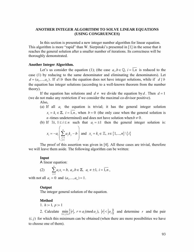
93
ANOTHER INTEGER ALGORITHM TO SOLVE LINEAR EQUATIONS
(USING CONGRUENCES) In this section is presented a new integer number algorithm for linear equation. This algorithm is more “rapid” than W. Sierpinski’s presented in [1] in the sense that it reaches the general solution after a smaller number of iterations. Its correctness will be thoroughly demonstrated. Another Integer Algorithm. Let’s us consider the equation (1); (the case ai ,b ∈Q, i = 1,n is reduced to the case (1) by reducing to the same denominator and eliminating the denominators). Let d = (a1,...,an ) . If d | b then the equation does not have integer solutions, while if |d b/ the equation has integer solutions (according to a well-known theorem from the number theory). If the equation has solutions and d ≠ we divide the equation by d . Then d = 1 (we do not make any restriction if we consider the maximal co-divisor positive). Also,
(a) If all ai the equation is trivial; it has the general integer solution
xi = ki ∈Z, i = 1,n , when b = 0 (the only case when the general solution is n -times undetermined) and does not have solution whenb ≠ 0 .
(b) If ∃i, 1 ≤ i ≤ n such that ai = ±1 then the general integer solution is:
xi = −ai ajk j − bj =1j ≠ i
n
∑⎛
⎝
⎜⎜
⎞
⎠
⎟⎟
and { } { }, 1,..., \s sx k s n i= ∈ ∈
The proof of this assertion was given in [4]. All these cases are trivial, therefore we will leave them aside. The following algorithm can be written: Input A linear equation:
(2)
aii=1
n
∑ xi = b, ai ,b ∈Z, ai ≠ ±1, i = 1,n ,
with not all ai = 0 and (a1,...,an ) = 1. Output The integer general solution of the equation. Method 1. h := 1, p := 1
2. Calculate { }1 ,min , (mod ), i j ji j n
r r a a r a≤ ≤
≡ < and determine r and the pair
(i, j) for which this minimum can be obtained (when there are more possibilities we have to choose one of them).
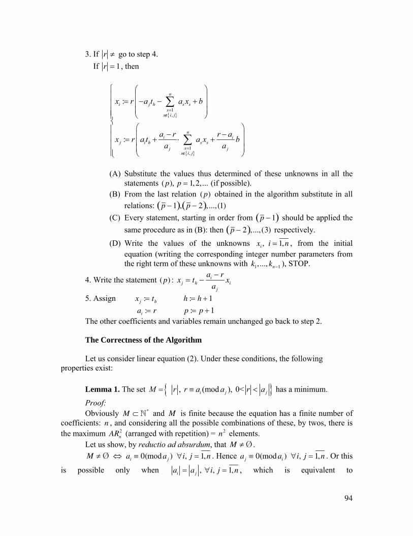
94
3. If r ≠ go to step 4. If r = 1 , then
{ }
{ }
1,
1,
:
:
n
i j h s ss
s i j
ni i
j i h s ssj j
s i j
x r a t a x b
a r r ax r a t a x ba a
=∉
=∉
⎧ ⎛ ⎞⎪ ⎜ ⎟= − − +⎪ ⎜ ⎟
⎜ ⎟⎪⎪ ⎝ ⎠⎨
⎛ ⎞⎪ − −⎜ ⎟⎪ = + ⋅ +⎜ ⎟⎪ ⎜ ⎟⎪ ⎝ ⎠⎩
∑
∑
(A) Substitute the values thus determined of these unknowns in all the
statements (p), p = 1,2,... (if possible). (B) From the last relation (p) obtained in the algorithm substitute in all
relations: p − 1( ), p − 2( ),...,(1) (C) Every statement, starting in order from p − 1( ) should be applied the
same procedure as in (B): then p − 2( ),...,(3) respectively.
(D) Write the values of the unknowns xi , i = 1,n , from the initial equation (writing the corresponding integer number parameters from the right term of these unknowns with k1,..., kn−1 ), STOP.
4. Write the statement (p) : xj = th −ai − r
aj
xi
5. Assign x j := th h := h + 1 ai := r p := p + 1 The other coefficients and variables remain unchanged go back to step 2.
The Correctness of the Algorithm Let us consider linear equation (2). Under these conditions, the following properties exist:
Lemma 1. The set { } , (mod ), 0<i j jM r r a a r a= ≡ < has a minimum.
Proof: Obviously M ⊂ N* and M is finite because the equation has a finite number of coefficients: n , and considering all the possible combinations of these, by twos, there is the maximum ARn
2 (arranged with repetition) = n2 elements. Let us show, by reductio ad absurdum, that M ≠ Ø . M ≠ Ø ⇔ ai ≡ 0(mod aj ) ∀i, j = 1,n . Hence aj ≡ 0(mod ai ) ∀i, j = 1,n . Or this
is possible only when ai = aj , ∀i, j = 1,n , which is equivalent to
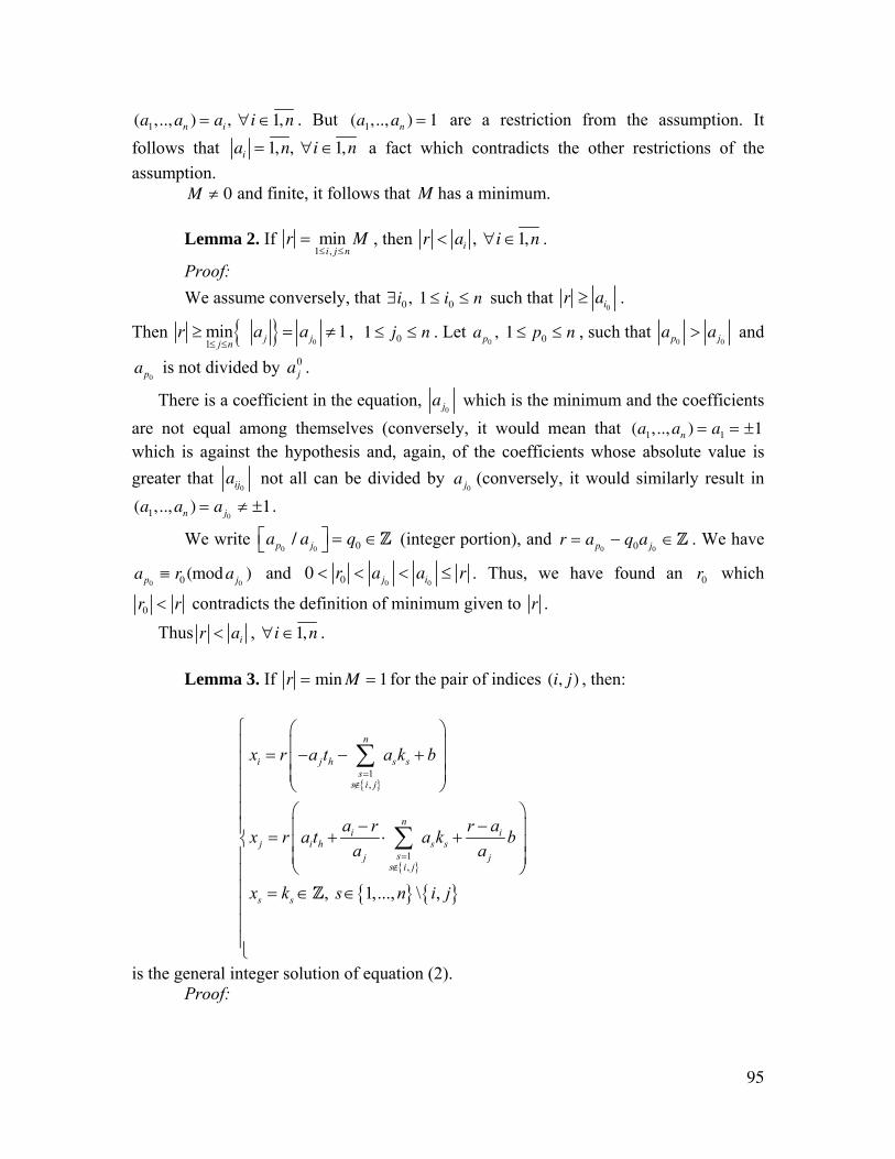
95
(a1,..,an ) = ai , ∀i ∈1,n . But (a1,..,an ) = 1 are a restriction from the assumption. It follows that ai = 1,n, ∀i ∈1,n a fact which contradicts the other restrictions of the assumption.
M ≠ 0 and finite, it follows that M has a minimum. Lemma 2. If r = min
1≤i, j ≤nM , then r < ai , ∀i ∈1,n .
Proof: We assume conversely, that ∃i0 , 1 ≤ i0 ≤ n such that r ≥ ai0
.
Then { } 01min 1j jj n
r a a≤ ≤
≥ = ≠ , 1 ≤ j0 ≤ n . Let ap0, 1 ≤ p0 ≤ n , such that ap0
> aj0 and
ap0 is not divided by aj
0 .
There is a coefficient in the equation, aj0 which is the minimum and the coefficients
are not equal among themselves (conversely, it would mean that (a1,..,an ) = a1 = ±1 which is against the hypothesis and, again, of the coefficients whose absolute value is greater that aij0
not all can be divided by aj0(conversely, it would similarly result in
(a1,..,an ) = aj0≠ ±1.
We write ap0/ aj0
⎡⎣ ⎤⎦ = q0 ∈Z (integer portion), and r = ap0− q0aj0
∈Z . We have
ap0≡ r0 (mod aj0
) and 0 < r0 < aj0< ai0
≤ r . Thus, we have found an r0 which
r0 < r contradicts the definition of minimum given to r .
Thus r < ai , ∀i ∈1,n . Lemma 3. If r = min M = 1 for the pair of indices (i, j) , then:
{ }
{ }
{ } { }
1,
1,
, 1,..., \ ,
n
i j h s ss
s i j
ni i
j i h s ssj j
s i j
s s
x r a t a k b
a r r ax r a t a k ba a
x k s n i j
=∉
=∉
⎧ ⎛ ⎞⎪ ⎜ ⎟= − − +⎪ ⎜ ⎟
⎜ ⎟⎪ ⎝ ⎠⎪⎛ ⎞⎪
− −⎪ ⎜ ⎟= + ⋅ +⎨ ⎜ ⎟⎪ ⎜ ⎟
⎝ ⎠⎪⎪ = ∈ ∈⎪⎪⎪⎩
∑
∑
Z
is the general integer solution of equation (2). Proof:
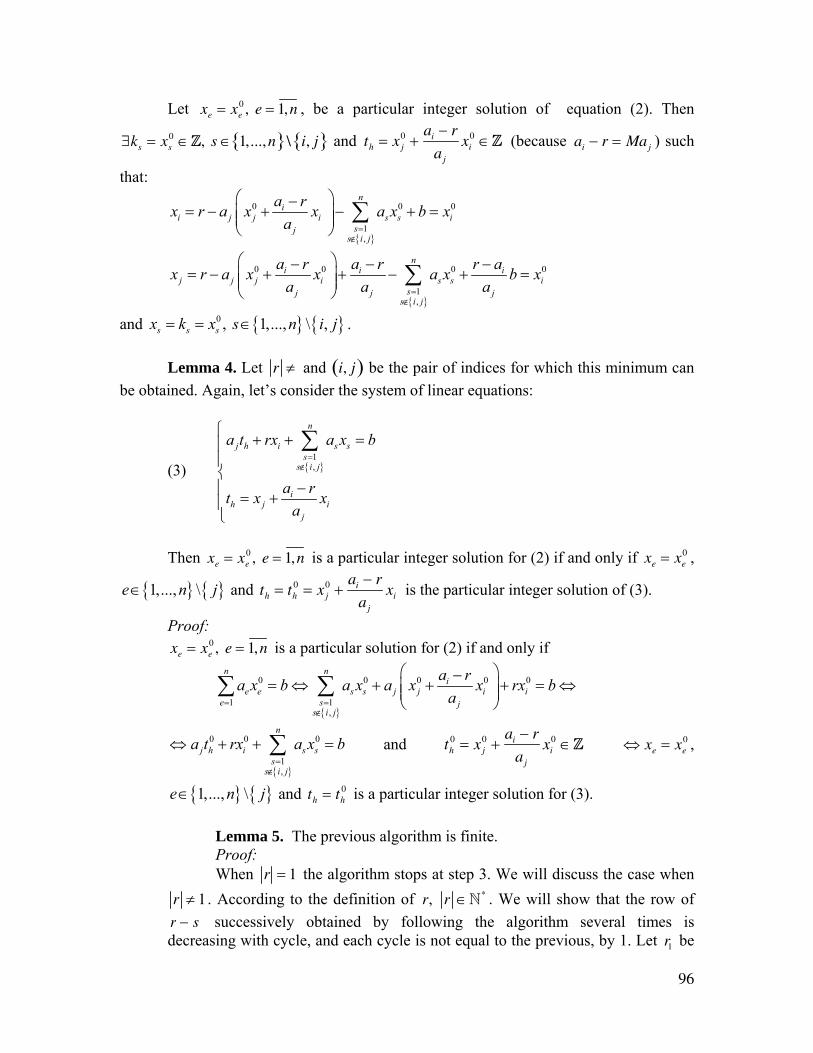
96
Let xe = xe0 , e = 1,n , be a particular integer solution of equation (2). Then
∃ks = xs0 ∈Z, s ∈ 1,...,n{ }\ i, j{ } and
th = x j
0 +ai − r
aj
xi0 ∈Z (because ai − r = Maj ) such
that:
{ }
0 0 0
1,
ni
i j j i s s isj
s i j
a rx r a x x a x b xa =
∉
⎛ ⎞−= − + − + =⎜ ⎟⎜ ⎟
⎝ ⎠∑
{ }
0 0 0 0
1,
ni i i
j j j i s s isj j j
s i j
a r a r r ax r a x x a x b xa a a=
∉
⎛ ⎞− − −= − + + − + =⎜ ⎟⎜ ⎟
⎝ ⎠∑
and { } { }0 , 1,..., \ ,s s sx k x s n i j= = ∈ . Lemma 4. Let r ≠ and i, j( ) be the pair of indices for which this minimum can be obtained. Again, let’s consider the system of linear equations:
(3) { } 1
,
n
j h i s ss
s i j
ih j i
j
a t rx a x b
a rt x xa
=∉
⎧ + + =⎪⎪⎨
−⎪ = +⎪⎩
∑
Then xe = xe
0 , e = 1,n is a particular integer solution for (2) if and only if xe = xe0 ,
{ } { }1,..., \e n j∈ and th = th0 = xj
0 +ai − r
aj
xi is the particular integer solution of (3).
Proof: xe = xe
0 , e = 1,n is a particular solution for (2) if and only if
{ }
0 0 0 0 0
1 1,
n ni
e e s s j j i ie s j
s i j
a ra x b a x a x x rx ba= =
∉
⎛ ⎞−= ⇔ + + + = ⇔⎜ ⎟⎜ ⎟
⎝ ⎠∑ ∑
{ }
0 0 0
1,
n
j h i s ss
s i j
a t rx a x b=
∉
⇔ + + =∑ and th
0 = xj0 +
ai − r
aj
xi0 ∈Z ⇔ xe = xe
0 ,
{ } { }1,..., \e n j∈ and th = th0 is a particular integer solution for (3).
Lemma 5. The previous algorithm is finite. Proof: When r = 1 the algorithm stops at step 3. We will discuss the case when r ≠ 1 . According to the definition of r, r ∈N* . We will show that the row of r − s successively obtained by following the algorithm several times is decreasing with cycle, and each cycle is not equal to the previous, by 1. Let r1 be
97
the first obtained by following the algorithm one time. r1 ≠ 1 then go to step 4,
and then step 5. According to lemma 2, r1 < ai , ∀i = 1,n . Now we shall follow the algorithm a second time, but this time for an
equation in which r1 (according to step 5) is substituted by ai . Again, according to lemma 2, the new r written r2 will have the propriety: r2 < r1 . We will get to r = 1 because r ≥ 1 and r < ∞ , and if r ≠ 1 , following the algorithm once again we get r < r1 and so on. Hence, the algorithm has a finite number of repetitions. Theorem of Correctness. The previous algorithm calculates the general solution of the linear equation correctly (2). Proof: According to lemma 5 the algorithm is finite. From lemma 1 it follows that the set M has a minimum, hence step 2 of the algorithm has meaning. When r = 1 it was shown in lemma 3 that step 3 of the algorithm calculates the general
integer solution of the respective equation correctly the equation that appears at step 3). In lemma 4 it is shown that if r ≠ 1 the substitutions steps 4 and 5 introduced in the initial equation, the general integer solution remains unchanged. That is, we pass from the initial equation to a linear system having the same general solution as the initial equation. The variable h is a counter of the newly introduced variables, which are used to successively decompose the system in systems of two linear equations. The variable p is a counter of the substitutions of variables (the relations, at a given moment between certain variables). When the initial equation was decomposed to r = 1 , we had to proceed in the reverse way, i.e. to compose its general integer solution. This reverse way is directed by the sub-steps 3(A), 3(B) and 3(C). The sub-step 3(D) has only an aesthetic role, i.e., to have the general solution under the form: xi = fi (k1 ,...,kn−1) , i = 1,n , fi being linear functions with integer number of coefficients. This “if possible” shows that substitutions are not always possible. But when they are we must make all possible substitutions. Note 1. The previous algorithm can be easily introduced into a computer program. Note 2. The previous algorithm is more “rapid” than that of W. Sierpinski’s [1], i.e., the general integer solution is reached after a smaller number of iterations (or, at least, the same) for any linear equation (2).
In the first place, both methods aim at obtaining the coefficient ±1 for at least one unknown variable. While Sierpinski started only by chance, decomposing the greatest coefficient in the module (writing it under the form of a sum between a multiple of the following smaller coefficient (in the module) and the rest), in our algorithm this decomposition is not accidental but always seeks the smallest r
98
and also choose the coefficients ai and aj for which this minimum is achieved. That is, we test from the beginning the shortest way to the general integer solution. Sierpinski does not attempt to find the shortest way; he knows that his method will take him to the general integer solution of the equation and is not interested in how long it will take. However, when an algorithm is introduced into a computer program it is preferable that the process time should be as short as possible.
Example 1. Let us solve in Z3 the equation 17x − 7y + 10z = −12 . We apply the former algorithm. 1. h = 1, p = 1 2. r = 3, i = 3, j = 2 3. 3 ≠ 1 go on to step 4.
4. (1) y = t1 −10 − 3
−7⋅ z = t1 + z
5. Assign
1
3
: : 2: 3 : 2
y t ha p
= == =
with the other coefficients and variables remaining unchanged, go back to step 2. 2. 1, 1, 3r i j= − = = 3. −1 = 1
x = −1(−3t2 − (−7t1) − 12) = 3t2 − 7t1 − 12
z = −1 17t2 + (−7t1) ⋅17 − (−1)
3+
−1 − 17
3(−12)
⎛⎝⎜
⎞⎠⎟
= 17t2 + 42t1 − 72
(A) We substitute the values of x and z thus determined into the only statement (p) we have: (1) 1 2 117 43 72y t z t t= + = − − + −
(B) The substitution is not possible. (C) The substitution is not possible. (D) The general integer solution of the equation is:
x = 3k1 − 7k2 + 12
y = −17k1 + 43k2 − 72
z = −17k1 + 42k2 − 72; k1, k2 ∈Z
⎧
⎨⎪
⎩⎪
REFERENCES:
99
[1] Sierpinski, W, - Ce ştim şi ce nu ştim despre numerele prime? - Editura Stiinţifică, Bucharest, 1966.
[2] Creangă, I., Cazacu, C., Mihuţ, P., Opaiţ, Gh., Corina Reisher – Introducere în teoria numerelor, Ed. Did. şi Ped., Bucharest, 1965.
[3] Popovici, C. P. – Aritmetica şi teoria numerelor, Ed. Did. şi Ped., Bucharest, 1963.
[4] Smarandache, Florentin – Un algoritm de rezolvare în numere întregi a ecuaţiilor liniare.
100
INTEGER NUMBER SOLUTIONS OF LINEAR SYSTEMS
Definitions and Properties of the Integer Solution of a Linear System
Let’s consider
(1) aijj =1
n
∑ xj = bi, i = 1,m
a linear system with all coefficients being integer numbers (the case with rational coefficients is reduced to the same). Definition 1. x j = x j
0 , j = 1,n , is a particular integer solution of (1) if
x j0 ∈Z, j = 1,n and aij x j
0
j =1
n
∑ = bi , i = 1,m .
Let’s consider the functions f j :Zh → Z, j = 1,n , where h ∈N* . Definition 2. x j = f j (k1,..., kh ), j = 1,n , is the general integer solution for (1) if:
(a) aij f j (k1,...,kh )j =1
n
∑ = bi , i = 1,m , irrespective of ( )1,..., hk k ∈Z ;
(b) Irrespective of xj = xj0 , j = 1,n a particular integer solution of (1) there is
0 01( ,..., )hk k ∈Z such that f j (k1
0 ,..., kh0 ) = x j , j = 1,n . (In other words the general solution
that comprises all the other solutions.) Property 1. A general solution of a linear system of m equations with n unknowns, r(A) = m < n , is undetermined ( )n m− -times. Proof: We assume by reduction ad absurdum that it is of order r , 1 ≤ r ≤ n − m (the case r = 0 , i.e., when the solution is particular, is trivial). It follows that the general solution is of the form:
(S1)
1 11 1 1 1
1 1
...:
... , , parameters
r r
n n nr r n ih
h
x u p u p v
x u p u p v u ip
= + + +⎧⎪⎪⎨ = + + + ∀ ∈⎪⎪ = ∈⎩
ZZ
We prove that the solution is undetermined ( )n m− -times. The homogeneous linear system (1), resolved in r has the solution:
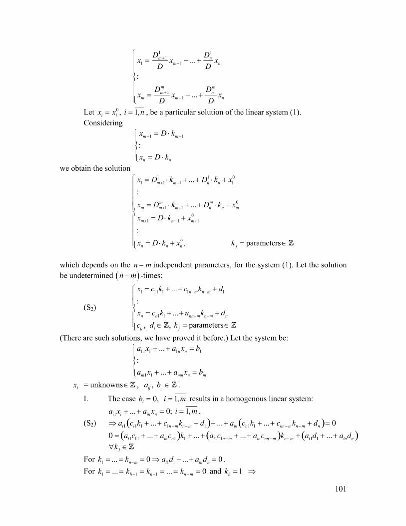
101
x1 =Dm+1
1
Dxm+1 + ...+
Dn1
Dxn
:
xm =Dm+1
m
Dxm+1 + ...+
Dnm
Dxn
⎧
⎨
⎪⎪
⎩
⎪⎪⎪
Let xi = xi0 , i = 1,n , be a particular solution of the linear system (1).
Considering
xm+1 = D ⋅ km+1
:
xn = D ⋅ kn
⎧
⎨⎪
⎩⎪
we obtain the solution
1 1 01 1 1 1
01 1
01 1 1
0
...:
...
:, parameters
m m n n
m mm m m n n m
m m m
n n n j
x D k D k x
x D k D k x
x D k x
x D k x k
+ +
+ +
+ + +
⎧ = ⋅ + + ⋅ +⎪⎪⎪ = ⋅ + + ⋅ +⎪⎨
= ⋅ +⎪⎪⎪
= ⋅ + = ∈⎪⎩ Z
which depends on the n − m independent parameters, for the system (1). Let the solution be undetermined ( )n m− -times:
(S2)
1 11 1 1 1
1 1
...:
..., , parameters
n m n m
n n nn m n m n
ij i j
x c k c k d
x c k u k dc d k
− −
− −
= + + +⎧⎪⎪⎨ = + + +⎪⎪ ∈ = ∈⎩ Z Z
(There are such solutions, we have proved it before.) Let the system be:
a11x1 + ... + a1nxn = b1
:
am1x1 + ... + amn xn = bm
⎧
⎨⎪
⎩⎪
xi = unknowns ∈Z , , iija b ∈Z .
I. The case bi = 0, i = 1, m results in a homogenous linear system: ai1xi + ... + ainxn = 0; i = 1, m . (S2) ⇒ ai1 ci1k1 + ... + c1n− mkn− m + d1( )+ ... + ain cn1k1 + ... + cnn− mkn− m + dn( )= 0
0 = ai1c11 + ... + aincn1( )k1 + ... + ai1c1n− m + ... + aincnn− m( )kn− m + ai1d1 + ... + aindn( ) ∀k j ∈Z
For 1 1 1... 0 ... 0n m i in nk k a d a d−= = = ⇒ + + = . For k1 = ... = kh−1 = kh+1 = ... = kn− m = 0 and 1 hk = ⇒
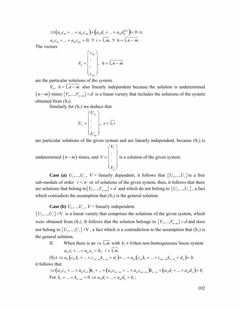
102
⇒ ai1cih + ... + aincnh( )+ ai1d1 + ... + aindd(n)( )= 0 ⇒
ai1cih + ... + aincnh = 0, ∀ i = 1, m, ∀ h = 1,n − m . The vectors
Vh =
c1h
:
:
cnh
⎛
⎝
⎜⎜⎜⎜
⎞
⎠
⎟⎟⎟⎟
, h = 1,n − m
are the particular solutions of the system. Vh , h = 1,n − m also linearly independent because the solution is undetermined ( )n m− -times { }1,..., n mV V d− + is a linear variety that includes the solutions of the system obtained from (S2).
Similarly for (S1) we deduce that
Us =
U1s
:
:
Uns
⎛
⎝
⎜⎜⎜⎜
⎞
⎠
⎟⎟⎟⎟
, s = 1,r
are particular solutions of the given system and are linearly independent, because (S1) is
undetermined ( )n m− -times, and V =
V1
:
:
Vn
⎛
⎝
⎜⎜⎜⎜
⎞
⎠
⎟⎟⎟⎟
is a solution of the given system.
Case (a) U1,...,Ur , V = linearly dependent, it follows that { }1,..., rU U is a free sub-module of order r < n - m of solutions of the given system, then, it follows that there are solutions that belong to{ }1,..., n mV V d− + and which do not belong to { }1,..., rU U , a fact which contradicts the assumption that (S1) is the general solution. Case (b) U1,...,Ur , V = linearly independent. { }1,..., +VrU U is a linear variety that comprises the solutions of the given system, which
were obtained from (S1). It follows that the solution belongs to { }1,..., n mV V d− + and does
not belong to { }1,..., +VrU U , a fact which is a contradiction to the assumption that (S1) is the general solution.
II. When there is an 1,i m∈ with bi ≠ 0 then non-homogeneous linear system ai1xi + ... + ainxn = b1, i = 1, m
(S2) ⇒ ai1 c11k1 + ... + c1n− mkn− m + d1( )+ ...+ ain cn1k1 + ... + cnn− mkn− m + dn( )= bi it follows that ⇒ ai1c11 + ... + aincn1( )k1 + ... + ai1c1n− m + ... + aincnn− m( )kn− m + ai1d1 + ... + aindn( )= bi For k1 = ... = kn− m = 0 1 1 1...i in na d a d b⇒ + + = ;
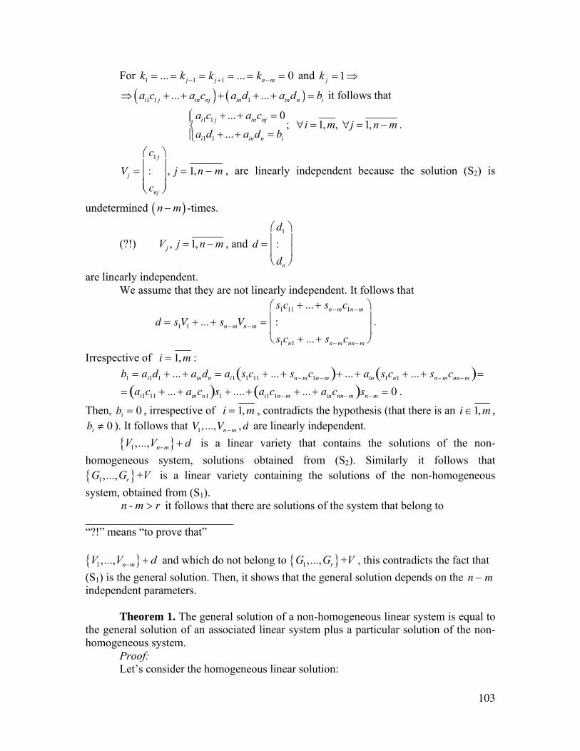
103
For k1 = ... = kj −1 = kj +1 = ... = kn− m = 0 and 1jk = ⇒
( ) ( )1 1 1... ...i j in nj in in n ia c a c a d a d b⇒ + + + + + = it follows that
1 1
1 1
... 0; 1, , 1,
...i j in nj
i in n i
a c a ci m j n m
a d a d b
+ + =⎧⎪ ∀ = ∀ = −⎨+ + =⎪⎩
.
Vj =
c1 j
:
cnj
⎛
⎝
⎜⎜⎜
⎞
⎠
⎟⎟⎟
, j = 1,n − m , are linearly independent because the solution (S2) is
undetermined ( )n m− -times.
(?!) , 1,jV j n m= − , and d =d1
:
dn
⎛
⎝
⎜⎜
⎞
⎠
⎟⎟
are linearly independent. We assume that they are not linearly independent. It follows that
d = s1V1 + ... + sn− mVn− m =s1c11 + ... + sn− mc1n− m
:
s1cn1 + ... + sn− mcnn− m
⎛
⎝
⎜⎜
⎞
⎠
⎟⎟
.
Irrespective of i = 1, m : b1 = ai1d1 + ... + aindn = ai1 s1c11 + ... + sn− mc1n− m( )+ ... + ain s1cn1 + ... + sn− mcnn− m( )=
= ai1c11 + ... + aincn1( )s1 + .... + ai1c1n− m + ... + aincnn− m( )sn− m = 0 .
Then, bi = 0 , irrespective of i = 1, m , contradicts the hypothesis (that there is an i ∈1, m , bi ≠ 0 ). It follows that V1,...,Vn− m , d are linearly independent. { }1,..., n mV V d− + is a linear variety that contains the solutions of the non-homogeneous system, solutions obtained from (S2). Similarly it follows that { }1,..., +rG G V is a linear variety containing the solutions of the non-homogeneous system, obtained from (S1). n - m > r it follows that there are solutions of the system that belong to __________________________ “?!” means “to prove that” { }1,..., n mV V d− + and which do not belong to { }1,..., +rG G V , this contradicts the fact that (S1) is the general solution. Then, it shows that the general solution depends on the n − m independent parameters. Theorem 1. The general solution of a non-homogeneous linear system is equal to the general solution of an associated linear system plus a particular solution of the non-homogeneous system. Proof: Let’s consider the homogeneous linear solution:
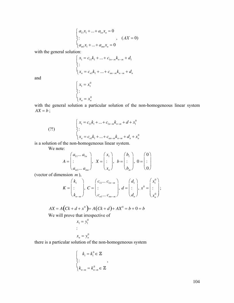
104
11 1 1
1 1
... 0: , ( 0)
... 0
n n
m mn n
a x a xAX
a x a x
+ + =⎧⎪ =⎨⎪ + + =⎩
with the general solution: x1 = c11k1 + ...+ c1n− mkn− m + d1
:
xn = cn1k1 + ... + cnn− mkn− m + dn
⎧
⎨⎪
⎩⎪
and
x1 = x1
0
:
xn = xn0
⎧
⎨⎪
⎩⎪
with the general solution a particular solution of the non-homogeneous linear system AX = b ;
(?!)
01 11 1 1 1
01 1
...:
...
n m n m
n n nn m n m n n
x c k c k d x
x c k c k d x
− −
− −
⎧ = + + + +⎪⎨⎪ = + + + +⎩
is a solution of the non-homogeneous linear system. We note:
A =a11... a1n
:
am1... amn
⎛
⎝
⎜⎜
⎞
⎠
⎟⎟
, X =x1
:
xn
⎛
⎝
⎜⎜
⎞
⎠
⎟⎟
, b =b1
:
bm
⎛
⎝
⎜⎜
⎞
⎠
⎟⎟
, 0 =0
:
0
⎛
⎝
⎜⎜
⎞
⎠
⎟⎟
(vector of dimension m ),
K =k1
:
kn− m
⎛
⎝
⎜⎜
⎞
⎠
⎟⎟
, C =c11... c1n− m
:
cn1... cnn− m
⎛
⎝
⎜⎜
⎞
⎠
⎟⎟
, d =d1
:
dn
⎛
⎝
⎜⎜
⎞
⎠
⎟⎟
, x0 =x1
0
:
xn0
⎛
⎝
⎜⎜⎜
⎞
⎠
⎟⎟⎟
;
AX = A Ck + d + x0( )= A Ck + d( )+ AX 0 = b + 0 = b We will prove that irrespective of
x1 = y1
0
:
xn = yn0
there is a particular solution of the non-homogeneous system
01 1
0
:
n m n m
k k
k k− −
⎧ = ∈⎪⎨⎪ = ∈⎩
Z
Z,
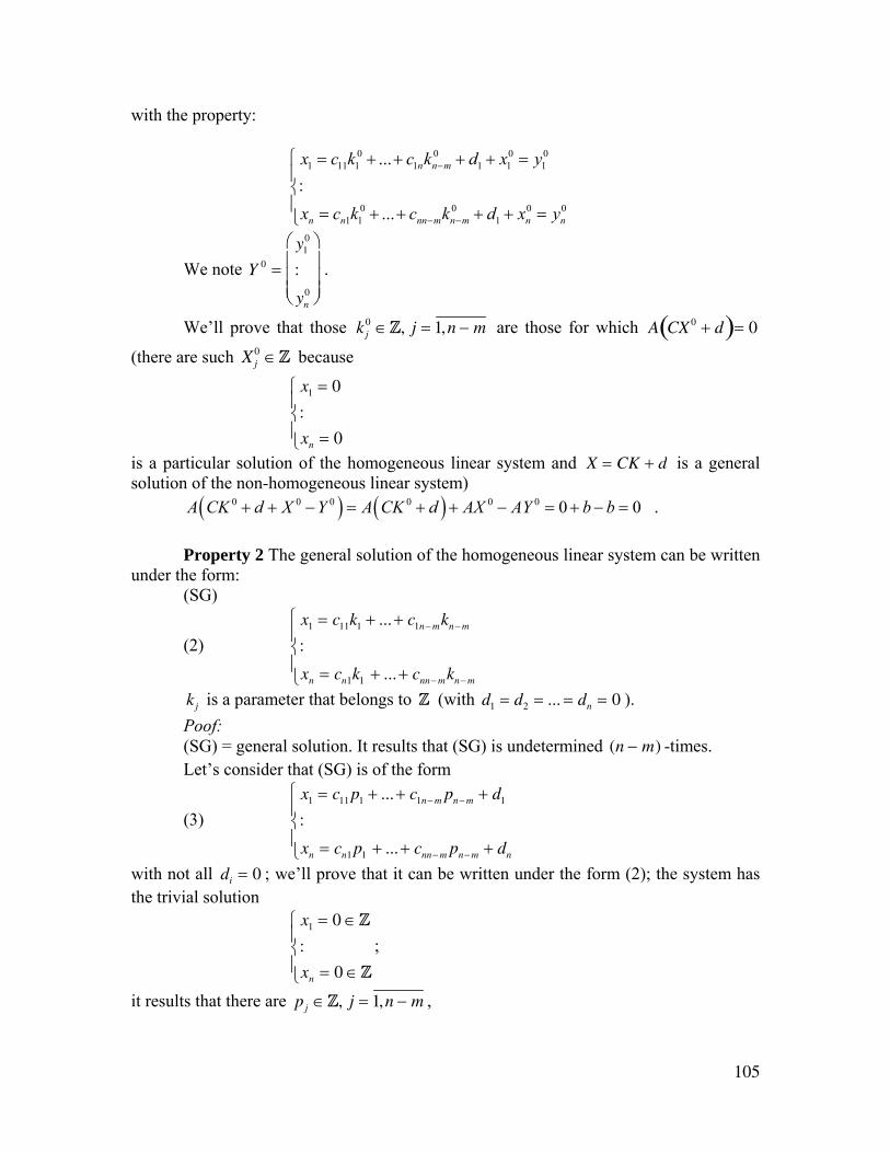
105
with the property:
0 0 0 01 11 1 1 1 1 1
0 0 0 01 1 1
...:
...
n n m
n n nn m n m n n
x c k c k d x y
x c k c k d x y
−
− −
⎧ = + + + + =⎪⎨⎪ = + + + + =⎩
We note Y 0 =y1
0
:
yn0
⎛
⎝
⎜⎜⎜
⎞
⎠
⎟⎟⎟
.
We’ll prove that those k j0 ∈Z, j = 1,n − m are those for which A CX 0 + d( )= 0
(there are such X j0 ∈Z because
x1 = 0
:
xn = 0
⎧
⎨⎪
⎩⎪
is a particular solution of the homogeneous linear system and X = CK + d is a general solution of the non-homogeneous linear system)
( ) ( )0 0 0 0 0 0 0 0 A CK d X Y A CK d AX AY b b+ + − = + + − = + − = .
Property 2 The general solution of the homogeneous linear system can be written under the form: (SG)
(2) x1 = c11k1 + ... + c1n− mkn− m
:
xn = cn1k1 + ... + cnn− mkn− m
⎧
⎨⎪
⎩⎪
kj is a parameter that belongs to Z (with d1 = d2 = ... = dn = 0 ). Poof: (SG) = general solution. It results that (SG) is undetermined (n − m) -times. Let’s consider that (SG) is of the form
(3) x1 = c11 p1 + ... + c1n− m pn− m + d1
:
xn = cn1 p1 + ... + cnn− m pn− m + dn
⎧
⎨⎪
⎩⎪
with not all di = 0 ; we’ll prove that it can be written under the form (2); the system has the trivial solution
x1 = 0 ∈Z:
xn = 0 ∈Z
⎧
⎨⎪
⎩⎪
;
it results that there are pj ∈Z, j = 1,n − m ,
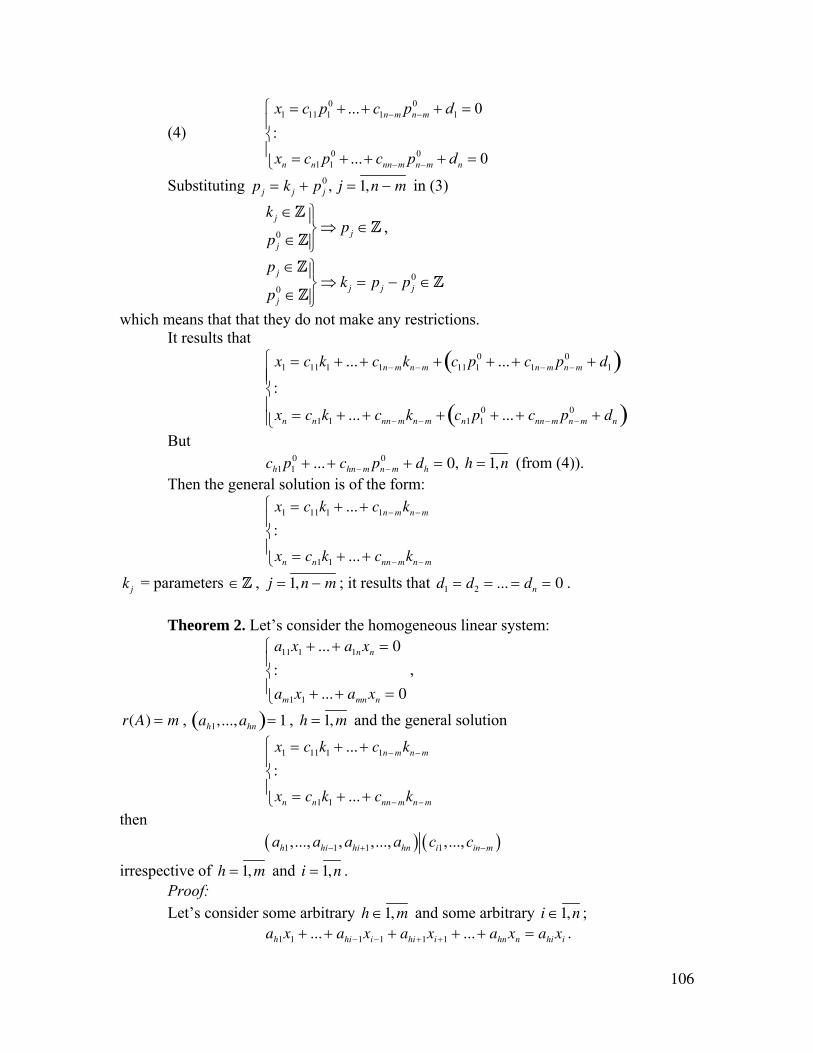
106
(4)
0 01 11 1 1 1
0 01 1
... 0:
... 0
n m n m
n n nn m n m n
x c p c p d
x c p c p d
− −
− −
⎧ = + + + =⎪⎨⎪ = + + + =⎩
Substituting pj = k j + pj0 , j = 1,n − m in (3)
kj ∈Z
pj0 ∈Z
⎫⎬⎪
⎭⎪⇒ pj ∈Z ,
pj ∈Z
pj0 ∈Z
⎫⎬⎪
⎭⎪⇒ kj = pj − pj
0 ∈Z
which means that that they do not make any restrictions. It results that
x1 = c11k1 + ...+ c1n− mkn− m + c11 p10 + ... + c1n− m pn− m
0 + d1( ):
xn = cn1k1 + ... + cnn− mkn− m + cn1 p10 + ... + cnn− m pn− m
0 + dn( )
⎧
⎨⎪⎪
⎩⎪⎪
But ch1 p1
0 + ... + chn− m pn− m0 + dh = 0, h = 1,n (from (4)).
Then the general solution is of the form:
x1 = c11k1 + ...+ c1n− mkn− m
:
xn = cn1k1 + ... + cnn− mkn− m
⎧
⎨⎪
⎩⎪
kj = parameters ∈Z , j = 1,n − m ; it results that d1 = d2 = ... = dn = 0 . Theorem 2. Let’s consider the homogeneous linear system:
a11x1 + ... + a1nxn = 0
:
am1x1 + ... + amnxn = 0
⎧
⎨⎪
⎩⎪
,
r(A) = m , ah1,...,ahn( )= 1 , h = 1, m and the general solution
x1 = c11k1 + ...+ c1n− mkn− m
:
xn = cn1k1 + ... + cnn− mkn− m
⎧
⎨⎪
⎩⎪
then ( ) ( )1 1 1 1,..., , ,..., ,...,h hi hi hn i in ma a a a c c− + −
irrespective of h = 1, m and i = 1,n . Proof: Let’s consider some arbitrary h ∈1, m and some arbitrary i ∈1,n ; ah1x1 + ... + ahi−1xi−1 + ahi+1xi+1 + ... + ahnxn = ahi xi .
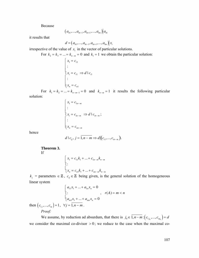
107
Because ( )1 1 1,..., , ,...,h hi hi hn hia a a a a− +
it results that ( )1 1 1,..., , ,...,h hi hi hn id a a a a x− +=
irrespective of the value of xi in the vector of particular solutions. For k2 = k3 = ... = kn− m = 0 and k1 = 1 we obtain the particular solution:
x1 = c11
:
xi = ci1
:
xn = cn1
⎧
⎨
⎪⎪⎪
⎩
⎪⎪⎪
⇒ d | ci1
For k1 = k2 = ... = kn− m−1 = 0 and kn− m = 1 it results the following particular solution:
x1 = c1n− m
:
xi = cin− m
:
xn = cnn− m
⎧
⎨
⎪⎪⎪
⎩
⎪⎪⎪
⇒ d | cin− m ;
hence d | cij , j = 1,n − m ⇒ d ci1,...,cin− m( ).
Theorem 3. If
x1 = c11k1 + ...+ c1n− mkn− m
:
xn = cn1k1 + ... + cnn− mkn− m
⎧
⎨⎪
⎩⎪
kj = parameters ∈Z , cij ∈Z being given, is the general solution of the homogeneous linear system
a11x1 + ... + a1nxn = 0
:
am1x1 + ... + amnxn = 0
⎧
⎨⎪
⎩⎪
, r(A) = m < n
then ( )1 ,..., 1j njc c = , ∀j = 1,n − m . Proof: We assume, by reduction ad absurdum, that there is ( )0 00 11, : ,...,j njj n m c c d∈ − =
we consider the maximal co-divisor > 0 ; we reduce to the case when the maximal co-
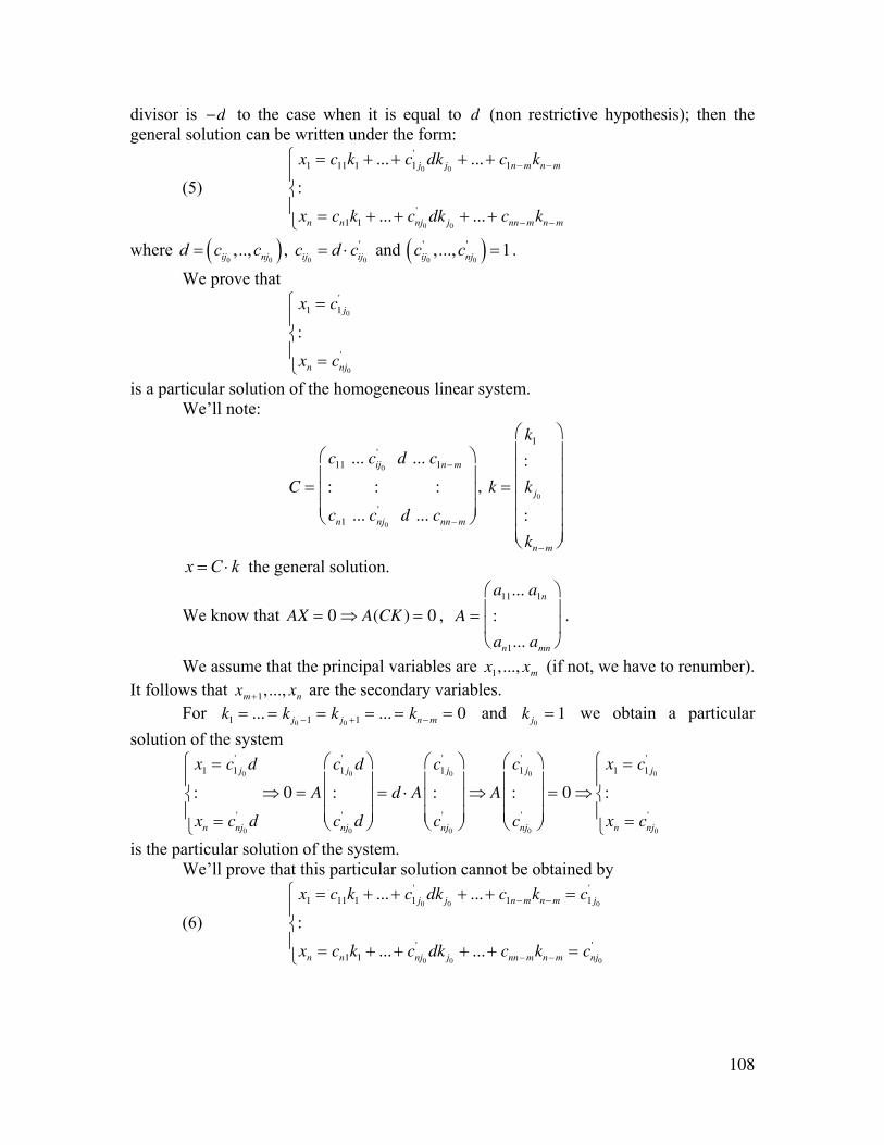
108
divisor is −d to the case when it is equal to d (non restrictive hypothesis); then the general solution can be written under the form:
(5)
x1 = c11k1 + ...+ c1 j0
' dkj0+ ...+ c1n− mkn− m
:
xn = cn1k1 + ...+ cnj0
' dkj0+ ...+ cnn− mkn− m
⎧
⎨⎪
⎩⎪
where ( )0 0 0 0
',.., , ij nj ij ijd c c c d c= = ⋅ and ( )0 0
' ',..., 1ij njc c = .
We prove that
x1 = c1 j0
'
:
xn = cnj0
'
⎧
⎨⎪
⎩⎪
is a particular solution of the homogeneous linear system. We’ll note:
C =
c11 ... cij0
' d ... c1n− m
: : :
cn1 ... cnj0
' d ... cnn− m
⎛
⎝
⎜⎜⎜
⎞
⎠
⎟⎟⎟
, k =
k1
:
kj0
:
kn− m
⎛
⎝
⎜⎜⎜⎜⎜⎜
⎞
⎠
⎟⎟⎟⎟⎟⎟
x C k= ⋅ the general solution.
We know that AX = 0 ⇒ A(CK ) = 0 , A =a11... a1n
:
an1... amn
⎛
⎝
⎜⎜
⎞
⎠
⎟⎟
.
We assume that the principal variables are x1,..., xm (if not, we have to renumber). It follows that xm +1,..., xn are the secondary variables. For k1 = ... = k j0 −1 = k j0 +1 = ... = kn− m = 0 and kj0
= 1 we obtain a particular solution of the system
x1 = c1 j0
' d
:
xn = cnj0
' d
⎧
⎨⎪
⎩⎪
⇒ 0 = A
c1 j0
' d
:
cnj0
' d
⎛
⎝
⎜⎜⎜
⎞
⎠
⎟⎟⎟
= d ⋅ A
c1 j0
'
:
cnj0
'
⎛
⎝
⎜⎜⎜
⎞
⎠
⎟⎟⎟
⇒ A
c1 j0
'
:
cnj0
'
⎛
⎝
⎜⎜⎜
⎞
⎠
⎟⎟⎟
= 0 ⇒
x1 = c1 j0
'
:
xn = cnj0
'
⎧
⎨⎪
⎩⎪
is the particular solution of the system. We’ll prove that this particular solution cannot be obtained by
(6)
x1 = c11k1 + ...+ c1 j0
' dkj0+ ...+ c1n− mkn− m = c1 j0
'
:
xn = cn1k1 + ...+ cnj0
' dkj0+ ...+ cnn− mkn− m = cnj0
'
⎧
⎨⎪
⎩⎪
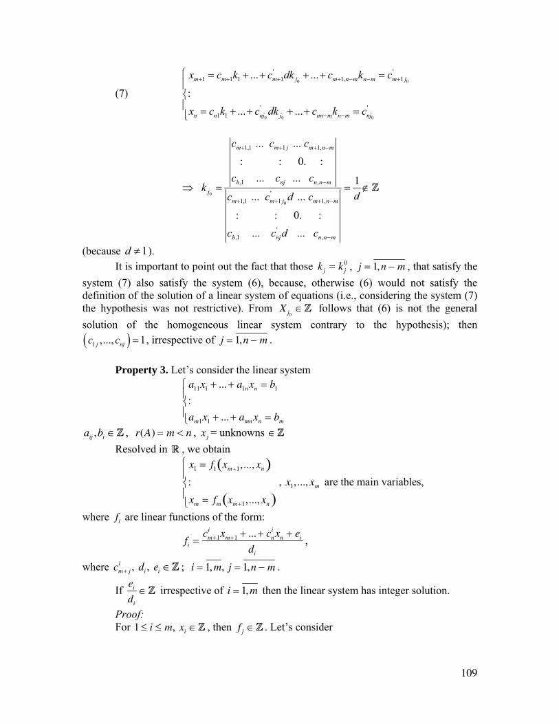
109
(7) 0 0
0 0 0
' '1 1 1 1 1, 1
' '1 1
... ...
:... ...
m m m j m n m n m m j
n n nj j nn m n m nj
x c k c dk c k c
x c k c dk c k c
+ + + + − − +
− −
⎧ = + + + + =⎪⎨⎪ = + + + + =⎩
0
0
1,1 1 1,
,1 ,
'1,1 1 1,
',1 ,
... ...
: : 0. : ... ...
... ...
: : 0. : ... ...
m m j m n m
h nj n n mj
m m j m n m
h nj n n
c c c
c c ck
c c d c
c c d c
+ + + −
−
+ + + −
⇒ =1
m
d
−
= ∉Z
(because 1d ≠ ). It is important to point out the fact that those kj = kj
0 , j = 1,n − m , that satisfy the system (7) also satisfy the system (6), because, otherwise (6) would not satisfy the definition of the solution of a linear system of equations (i.e., considering the system (7) the hypothesis was not restrictive). From X j0
∈Z follows that (6) is not the general solution of the homogeneous linear system contrary to the hypothesis); then ( )1 ,..., 1j njc c = , irrespective of j = 1,n − m . Property 3. Let’s consider the linear system
a11x1 + ... + a1nxn = b1
:
am1x1 + ... + amn xn = bm
⎧
⎨⎪
⎩⎪
aij ,bi ∈Z , r(A) = m < n , xj = unknowns ∈Z Resolved in R , we obtain
x1 = f1 xm+1,..., xn( ):
xm = fm xm+1,..., xn( )
⎧
⎨⎪
⎩⎪
, x1,..., xm are the main variables,
where fi are linear functions of the form:
fi =cm+1
i xm+1 + ...+ cni xn + ei
di
,
where cm+ ji , di , ei ∈Z ; i = 1, m, j = 1,n − m .
If
ei
di
∈Z irrespective of i = 1,m then the linear system has integer solution.
Proof: For 1 ≤ i ≤ m, xi ∈Z , then f j ∈Z . Let’s consider
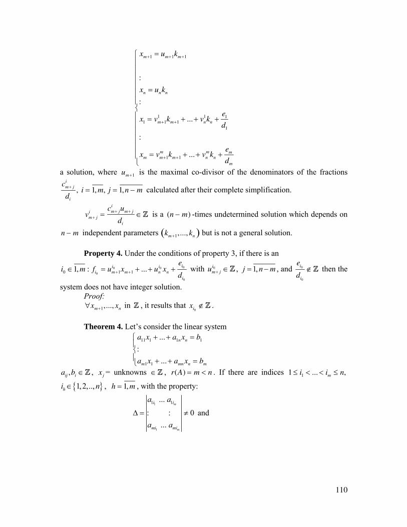
110
xm+1 = um+1km+1
:
xn = unkn
:
x1 = vm+11 km+1 + ...+ vn
1kn +e1
d1
:
xm = vm+1m km+1 + ...+ vn
mkn +em
dm
⎧
⎨
⎪⎪⎪⎪⎪⎪
⎩
⎪⎪⎪⎪⎪⎪
a solution, where um +1 is the maximal co-divisor of the denominators of the fractions cm+ j
i
di
, i = 1, m, j = 1,n − m calculated after their complete simplification.
vm+ j
i =cm+ j
i um+ j
di
∈Z is a (n − m) -times undetermined solution which depends on
n − m independent parameters km +1,..., kn( ) but is not a general solution. Property 4. Under the conditions of property 3, if there is an
i0 ∈1, m : fi0= um+1
i0 xm +1 + ... + uni0 xn +
ei0
di0
with um+ ji0 ∈Z , 1,j n m= − , and
ei0
di0
∉Z then the
system does not have integer solution. Proof: ∀xm+1,..., xn in Z , it results that xi0
∉Z . Theorem 4. Let’s consider the linear system
a11x1 + ... + a1nxn = b1
:
am1x1 + ... + amn xn = bm
⎧
⎨⎪
⎩⎪
aij ,bi ∈Z , xj = unknowns ∈Z , r(A) = m < n . If there are indices 1 ≤ i1 < ... < im ≤ n,
{ }1,2,..,hi n∈ , h = 1, m , with the property:
1
1
1 1 ...
: : 0 ...
m
m
i i
mi mi
a a
a aΔ = ≠ and
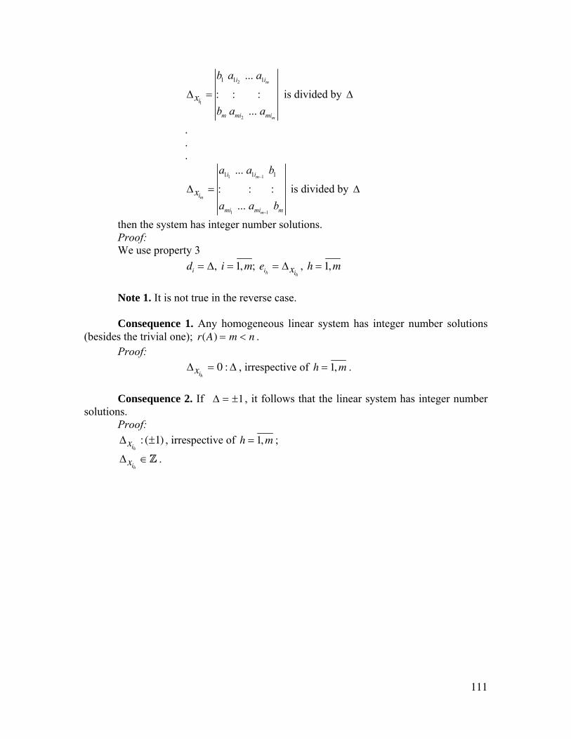
111
2
1
2
1 1 1
...
: : : ...
m
m
i i
m mi mi
ix
b a a
b a aΔ = is divided by Δ
. . .
1 1
1 1
1 1 1...
: : :...
m
m
m
i i
mi mi m
ix
a a b
a a b
−
−
Δ = is divided by Δ
then the system has integer number solutions. Proof: We use property 3
di = Δ, i = 1,m; eih= Δxih
, h = 1,m
Note 1. It is not true in the reverse case. Consequence 1. Any homogeneous linear system has integer number solutions
(besides the trivial one); r(A) = m < n . Proof:
Δxih= 0 : Δ , irrespective of h = 1, m .
Consequence 2. If Δ = ±1 , it follows that the linear system has integer number
solutions. Proof: Δxih
: (±1) , irrespective of h = 1, m ;
Δxih
∈Z .
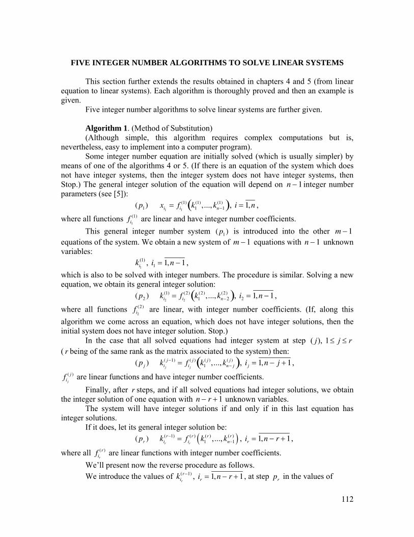
112
FIVE INTEGER NUMBER ALGORITHMS TO SOLVE LINEAR SYSTEMS
This section further extends the results obtained in chapters 4 and 5 (from linear equation to linear systems). Each algorithm is thoroughly proved and then an example is given. Five integer number algorithms to solve linear systems are further given. Algorithm 1. (Method of Substitution) (Although simple, this algorithm requires complex computations but is, nevertheless, easy to implement into a computer program). Some integer number equation are initially solved (which is usually simpler) by means of one of the algorithms 4 or 5. (If there is an equation of the system which does not have integer systems, then the integer system does not have integer systems, then Stop.) The general integer solution of the equation will depend on n − 1 integer number parameters (see [5]):
(p1) xi1= fi1
(1) k1(1),..., kn−1
(1)( ), i = 1,n ,
where all functions fi1
(1) are linear and have integer number coefficients. This general integer number system (p1) is introduced into the other m − 1 equations of the system. We obtain a new system of m − 1 equations with n − 1 unknown variables:
1
(1)ik , i1 = 1,n − 1 ,
which is also to be solved with integer numbers. The procedure is similar. Solving a new equation, we obtain its general integer solution:
( p2 ) ki2
(1) = fi2
(2) k1(2),..., kn−2
(2)( ), i2 = 1,n − 1 ,
where all functions fi2
(2) are linear, with integer number coefficients. (If, along this algorithm we come across an equation, which does not have integer solutions, then the initial system does not have integer solution. Stop.) In the case that all solved equations had integer system at step ( ), 1j j r≤ ≤ ( r being of the same rank as the matrix associated to the system) then: ( pj ) kij
( j −1) = fi j
( j ) k1( j ),..., kn− j
( j )( ), i j = 1,n − j + 1 ,
fi j
( j ) are linear functions and have integer number coefficients. Finally, after r steps, and if all solved equations had integer solutions, we obtain the integer solution of one equation with n − r + 1 unknown variables. The system will have integer solutions if and only if in this last equation has integer solutions. If it does, let its general integer solution be:
( pr ) ( )( 1) ( ) ( ) ( )1 1,...,
r r
r r r ri i nk f k k−
−= , ir = 1,n − r + 1 ,
where all fir
(r ) are linear functions with integer number coefficients. We’ll present now the reverse procedure as follows. We introduce the values of kir
(r −1) , ir = 1,n − r + 1 , at step pr in the values of
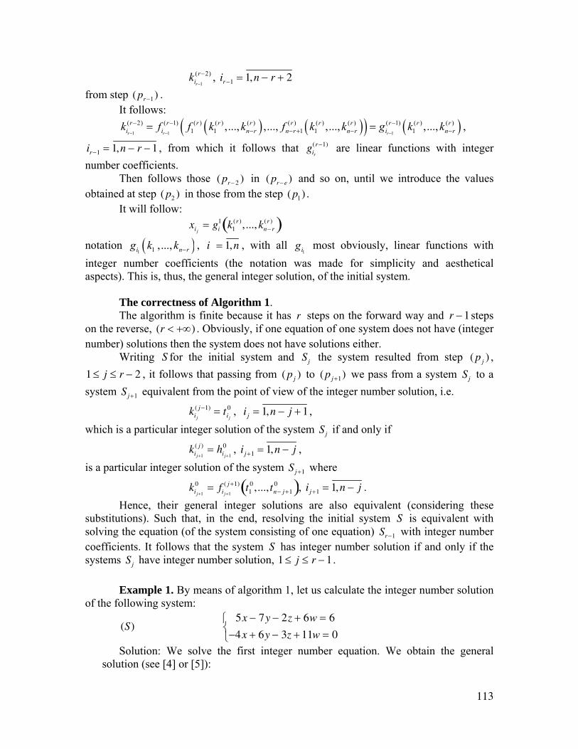
113
1
( 2)r
rik
−
− , ir −1 = 1,n − r + 2 from step (pr −1) . It follows: ( ) ( )( ) ( )
1 1 1
( 2) ( 1) ( ) ( ) ( ) ( ) ( ) ( ) ( 1) ( ) ( )1 1 1 1 1,..., ,..., ,..., ,...,
r r r
r r r r r r r r r r ri i n r n r n r i n rk f f k k f k k g k k
− − −
− − −− − + − −= = ,
ir −1 = 1,n − r − 1 , from which it follows that gir
(r−1) are linear functions with integer number coefficients. Then follows those ( pr − 2 ) in (pr −e ) and so on, until we introduce the values obtained at step ( p2 ) in those from the step (p1) . It will follow: xij
= gi1 k1
(r ),..., kn− r(r )( )
notation ( )1 1 ,...,i n rg k k − , i = 1,n , with all
1ig most obviously, linear functions with
integer number coefficients (the notation was made for simplicity and aesthetical aspects). This is, thus, the general integer solution, of the initial system. The correctness of Algorithm 1. The algorithm is finite because it has r steps on the forward way and r − 1steps on the reverse, (r < +∞) . Obviously, if one equation of one system does not have (integer number) solutions then the system does not have solutions either. Writing S for the initial system and Sj the system resulted from step ( pj ) , 1 ≤ j ≤ r − 2 , it follows that passing from ( pj ) to (pj +1) we pass from a system Sj to a system Sj +1 equivalent from the point of view of the integer number solution, i.e.
kij
( j −1) = tij
0 , i j = 1,n − j + 1 , which is a particular integer solution of the system Sj if and only if
kij+1
( j ) = hij+1
0 , i j +1 = 1,n − j , is a particular integer solution of the system Sj +1 where
kij+1
0 = fi j+1
( j +1) t10 ,...,tn− j +1
0( ), i j +1 = 1,n − j . Hence, their general integer solutions are also equivalent (considering these substitutions). Such that, in the end, resolving the initial system S is equivalent with solving the equation (of the system consisting of one equation) Sr −1 with integer number coefficients. It follows that the system S has integer number solution if and only if the systems Sj have integer number solution, 1 ≤ j ≤ r − 1 . Example 1. By means of algorithm 1, let us calculate the integer number solution of the following system:
(S) 5x − 7y − 2z + 6w = 6
−4x + 6y − 3z + 11w = 0
⎧⎨⎩
Solution: We solve the first integer number equation. We obtain the general solution (see [4] or [5]):
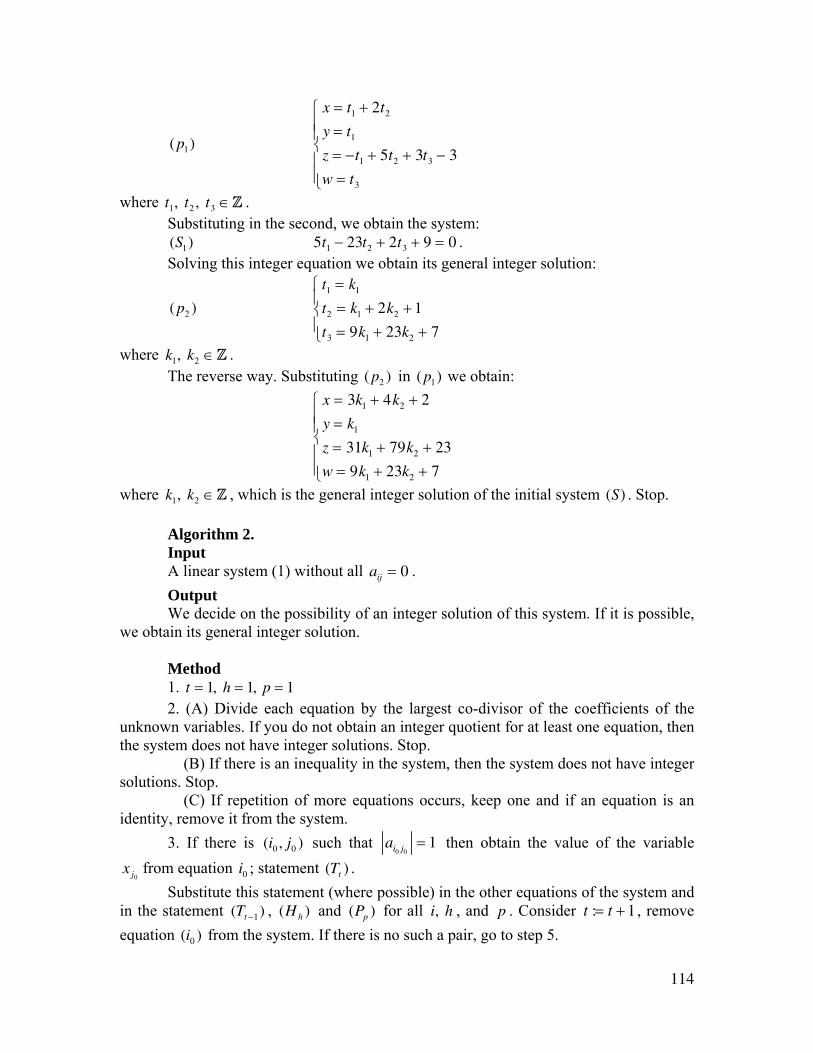
114
(p1)
x = t1 + 2t2
y = t1
z = −t1 + 5t2 + 3t3 − 3
w = t3
⎧
⎨⎪⎪
⎩⎪⎪
where t1, t2 , t3 ∈Z . Substituting in the second, we obtain the system:
(S1) 5t1 − 23t2 + 2t3 + 9 = 0 . Solving this integer equation we obtain its general integer solution:
( p2 ) t1 = k1
t2 = k1 + 2k2 + 1
t3 = 9k1 + 23k2 + 7
⎧
⎨⎪
⎩⎪
where k1, k2 ∈Z . The reverse way. Substituting ( p2 ) in (p1) we obtain:
x = 3k1 + 4k2 + 2
y = k1
z = 31k1 + 79k2 + 23
w = 9k1 + 23k2 + 7
⎧
⎨⎪⎪
⎩⎪⎪
where k1, k2 ∈Z , which is the general integer solution of the initial system (S) . Stop. Algorithm 2. Input A linear system (1) without all aij = 0 . Output We decide on the possibility of an integer solution of this system. If it is possible, we obtain its general integer solution. Method 1. t = 1, h = 1, p = 1 2. (A) Divide each equation by the largest co-divisor of the coefficients of the unknown variables. If you do not obtain an integer quotient for at least one equation, then the system does not have integer solutions. Stop. (B) If there is an inequality in the system, then the system does not have integer solutions. Stop. (C) If repetition of more equations occurs, keep one and if an equation is an identity, remove it from the system. 3. If there is (i0 , j0 ) such that ai0 j0
= 1 then obtain the value of the variable x j0
from equation i0 ; statement (Tt ) . Substitute this statement (where possible) in the other equations of the system and in the statement (Tt −1) , (H h ) and (Pp ) for all i, h , and p . Consider t := t + 1 , remove equation (i0 ) from the system. If there is no such a pair, go to step 5.
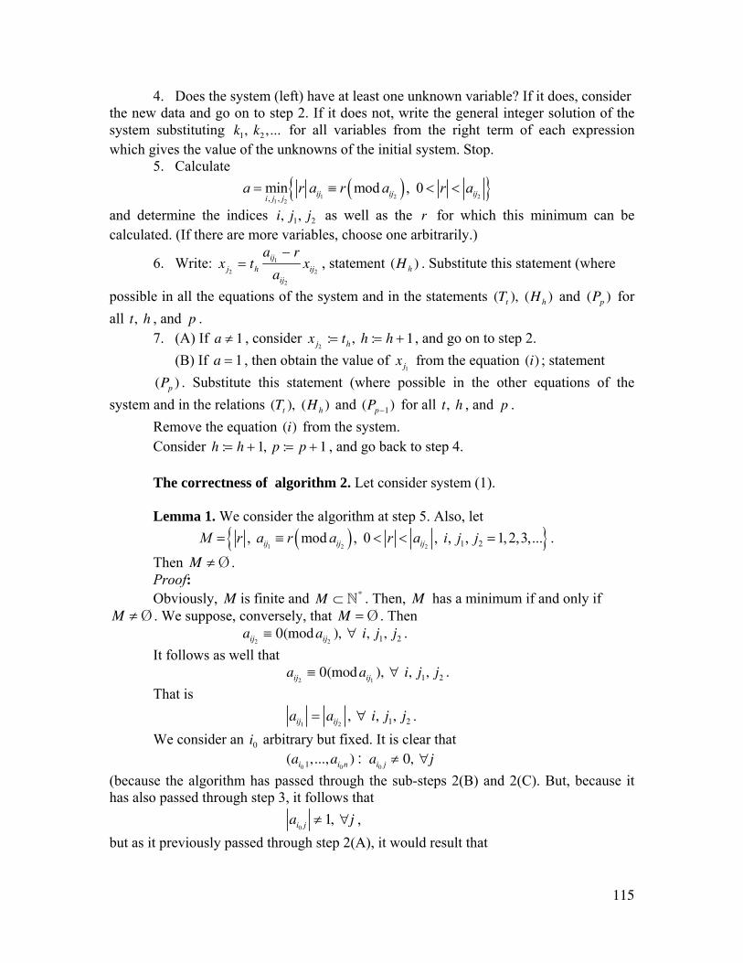
115
4. Does the system (left) have at least one unknown variable? If it does, consider the new data and go on to step 2. If it does not, write the general integer solution of the system substituting k1, k2 ,... for all variables from the right term of each expression which gives the value of the unknowns of the initial system. Stop.
5. Calculate ( ){ }1 2 2
1 2, ,min mod , 0ij ij iji j j
a r a r a r a= ≡ < <
and determine the indices i, j1, j2 as well as the r for which this minimum can be calculated. (If there are more variables, choose one arbitrarily.)
6. Write: x j2= th
aij1− r
aij2
xij2, statement (H h ) . Substitute this statement (where
possible in all the equations of the system and in the statements (Tt ), (Hh ) and (Pp ) for all t, h , and p .
7. (A) If a ≠ 1 , consider x j2:= th , h := h + 1 , and go on to step 2.
(B) If a = 1 , then obtain the value of xj1 from the equation (i) ; statement
(Pp ) . Substitute this statement (where possible in the other equations of the system and in the relations (Tt ), (Hh ) and (Pp−1) for all t, h , and p .
Remove the equation (i) from the system. Consider h := h + 1, p := p + 1 , and go back to step 4. The correctness of algorithm 2. Let consider system (1). Lemma 1. We consider the algorithm at step 5. Also, let
( ){ }1 2 2 1 2, mod , 0 , , , 1, 2,3,...ij ij ijM r a r a r a i j j= ≡ < < = .
Then M ≠ Ø . Proof: Obviously, M is finite and M ⊂ N* . Then, M has a minimum if and only if
M ≠ Ø . We suppose, conversely, that M = Ø . Then aij2
≡ 0(mod aij2), ∀ i, j1, j2 .
It follows as well that aij2
≡ 0(mod aij1), ∀ i, j1, j2 .
That is aij1
= aij2, ∀ i, j1, j2 .
We consider an i0 arbitrary but fixed. It is clear that
(ai0 1,...,ai0 n ) : ai0 j ≠ 0, ∀j (because the algorithm has passed through the sub-steps 2(B) and 2(C). But, because it has also passed through step 3, it follows that
ai0 j ≠ 1, ∀j , but as it previously passed through step 2(A), it would result that
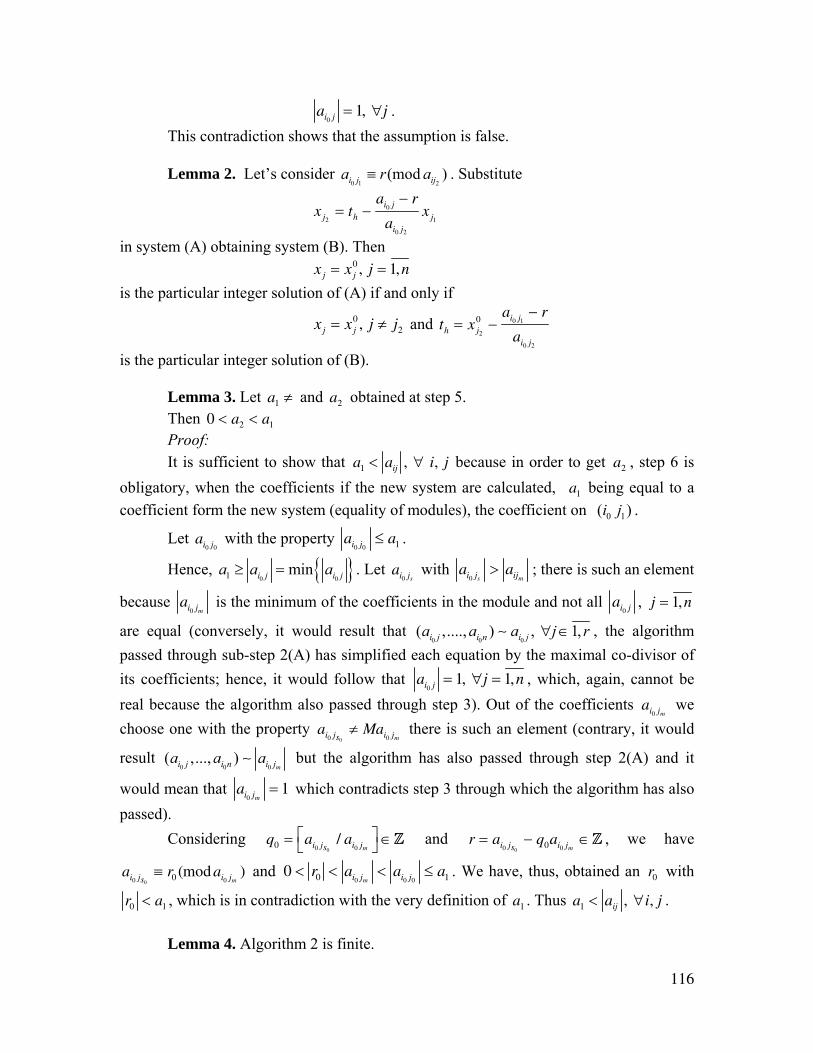
116
ai0 j = 1, ∀j . This contradiction shows that the assumption is false. Lemma 2. Let’s consider
0 1 2(mod )i j ija r a≡ . Substitute
x j2= th −
ai0 j − r
ai0 j2
x j1
in system (A) obtaining system (B). Then x j = x j
0 , j = 1,n is the particular integer solution of (A) if and only if
xj = xj0, j ≠ j2 and th = x j2
0 −ai0 j1
− r
ai0 j2
is the particular integer solution of (B). Lemma 3. Let a1 ≠ and a2 obtained at step 5. Then 0 < a2 < a1 Proof: It is sufficient to show that a1 < aij , ∀ i, j because in order to get a2 , step 6 is obligatory, when the coefficients if the new system are calculated, a1 being equal to a coefficient form the new system (equality of modules), the coefficient on 0 1 ( )i j .
Let ai0 j0 with the property ai0 j0
≤ a1 .
Hence, { }0 01 mini j i ja a a≥ = . Let ai0 js with ai0 js
> aijm; there is such an element
because ai0 jm is the minimum of the coefficients in the module and not all ai0 j , j = 1,n
are equal (conversely, it would result that 0 0 0
( ,...., ) , 1,i j i n i ja a a j r∀ ∈∼ , the algorithm passed through sub-step 2(A) has simplified each equation by the maximal co-divisor of its coefficients; hence, it would follow that ai0 j = 1, ∀j = 1,n , which, again, cannot be real because the algorithm also passed through step 3). Out of the coefficients ai0 jm
we choose one with the property ai0 js0
≠ Mai0 jm there is such an element (contrary, it would
result 0 0 0
( ,..., )mi j i n i ja a a∼ but the algorithm has also passed through step 2(A) and it
would mean that ai0 jm= 1 which contradicts step 3 through which the algorithm has also
passed). Considering
q0 = ai0 js0
/ ai0 jm⎡⎣
⎤⎦ ∈Z and r = ai0 js0
− q0ai0 jm∈Z , we have
ai0 js0
≡ r0 (mod ai0 jm) and 0 < r0 < ai0 jm
< ai0 j0≤ a1 . We have, thus, obtained an r0 with
r0 < a1 , which is in contradiction with the very definition of a1 . Thus a1 < aij , ∀i, j . Lemma 4. Algorithm 2 is finite.
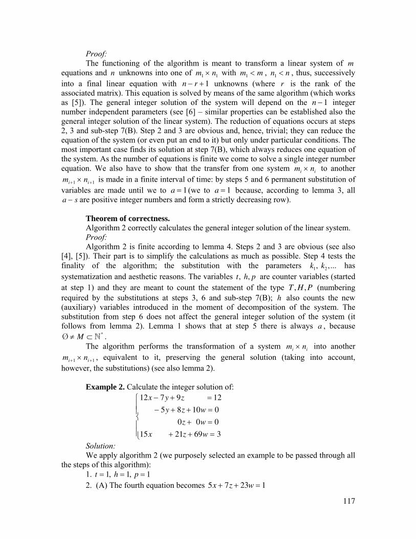
117
Proof: The functioning of the algorithm is meant to transform a linear system of m equations and n unknowns into one of m1 × n1 with m1 < m , n1 < n , thus, successively into a final linear equation with n − r + 1 unknowns (where r is the rank of the associated matrix). This equation is solved by means of the same algorithm (which works as [5]). The general integer solution of the system will depend on the n − 1 integer number independent parameters (see [6] – similar properties can be established also the general integer solution of the linear system). The reduction of equations occurs at steps 2, 3 and sub-step 7(B). Step 2 and 3 are obvious and, hence, trivial; they can reduce the equation of the system (or even put an end to it) but only under particular conditions. The most important case finds its solution at step 7(B), which always reduces one equation of the system. As the number of equations is finite we come to solve a single integer number equation. We also have to show that the transfer from one system mi × ni to another mi+1 × ni+1 is made in a finite interval of time: by steps 5 and 6 permanent substitution of variables are made until we to a = 1 (we to a = 1 because, according to lemma 3, all a − s are positive integer numbers and form a strictly decreasing row). Theorem of correctness.
Algorithm 2 correctly calculates the general integer solution of the linear system. Proof: Algorithm 2 is finite according to lemma 4. Steps 2 and 3 are obvious (see also [4], [5]). Their part is to simplify the calculations as much as possible. Step 4 tests the finality of the algorithm; the substitution with the parameters k1, k2 ,... has systematization and aesthetic reasons. The variables t, h, p are counter variables (started at step 1) and they are meant to count the statement of the type T , H ,P (numbering required by the substitutions at steps 3, 6 and sub-step 7(B); h also counts the new (auxiliary) variables introduced in the moment of decomposition of the system. The substitution from step 6 does not affect the general integer solution of the system (it follows from lemma 2). Lemma 1 shows that at step 5 there is always a , because Ø ≠ M ⊂ N* . The algorithm performs the transformation of a system mi × ni into another mi +1 × ni +1 , equivalent to it, preserving the general solution (taking into account, however, the substitutions) (see also lemma 2). Example 2. Calculate the integer solution of:
12x − 7y + 9z = 12
− 5y + 8z + 10w = 0
0z + 0w = 0
15x + 21z + 69w = 3
⎧
⎨⎪⎪
⎩⎪⎪
Solution: We apply algorithm 2 (we purposely selected an example to be passed through all the steps of this algorithm): 1. t = 1, h = 1, p = 1 2. (A) The fourth equation becomes 5x + 7z + 23w = 1
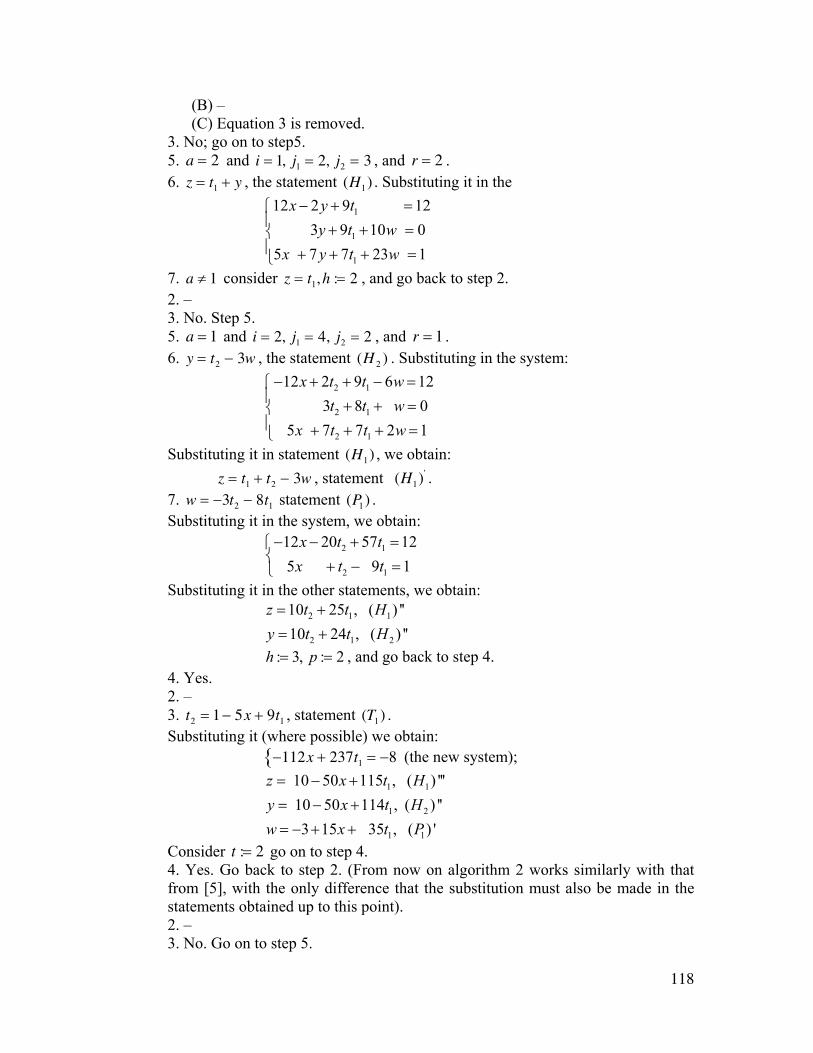
118
(B) – (C) Equation 3 is removed. 3. No; go on to step5. 5. a = 2 and i = 1, j1 = 2, j2 = 3 , and r = 2 . 6. z = t1 + y , the statement (H1) . Substituting it in the
1
1
1
12 2 9 12 3 9 10 05 7 7 23 1
x y ty t w
x y t w
− + =⎧⎪ + + =⎨⎪ + + + =⎩
7. a ≠ 1 consider z = t1,h := 2 , and go back to step 2. 2. – 3. No. Step 5. 5. a = 1 and i = 2, j1 = 4, j2 = 2 , and r = 1 .
6. y = t2 − 3w , the statement (H 2 ) . Substituting in the system:
2 1
2 1
2 1
12 2 9 6 12 3 8 0 5 7 7 2 1
x t t wt t w
x t t w
− + + − =⎧⎪ + + =⎨⎪ + + + =⎩
Substituting it in statement (H1) , we obtain: z = t1 + t2 − 3w , statement (H1)' . 7. w = −3t2 − 8t1 statement (P1) . Substituting it in the system, we obtain:
2 1
2 1
12 20 57 12 5 9 1
x t tx t t
− − + =⎧⎨ + − =⎩
Substituting it in the other statements, we obtain:
2 1 1
2 1 2
10 25 , ( ) ''10 24 , ( ) ''
z t t Hy t t H
= += +
: 3, : 2h p= = , and go back to step 4. 4. Yes. 2. – 3. t2 = 1 − 5x + 9t1 , statement (T1) . Substituting it (where possible) we obtain: −112x + 237t1 = −8{ (the new system);
1 1
1 2
1 1
10 50 115 , ( ) ''' 10 50 114 , ( ) ''
3 15 35 , ( ) '
z x t Hy x t Hw x t P
= − += − += − + +
Consider t := 2 go on to step 4. 4. Yes. Go back to step 2. (From now on algorithm 2 works similarly with that from [5], with the only difference that the substitution must also be made in the statements obtained up to this point). 2. – 3. No. Go on to step 5.
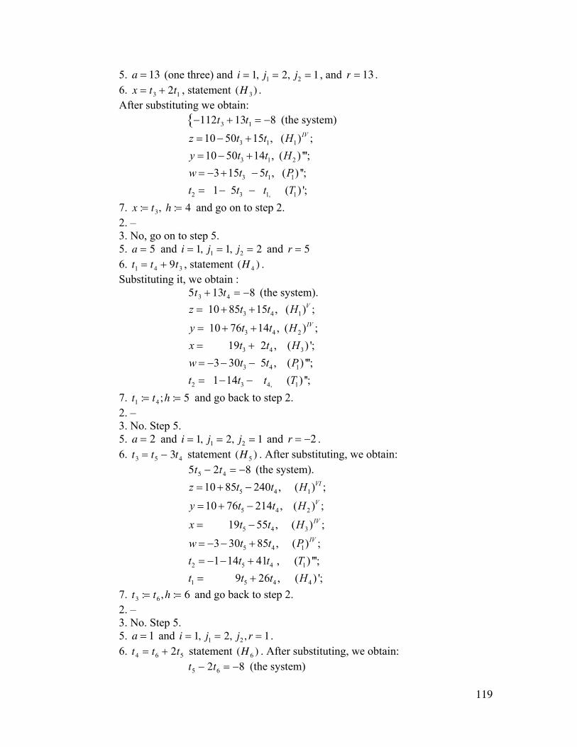
119
5. a = 13 (one three) and i = 1, j1 = 2, j2 = 1 , and r = 13 . 6. x = t3 + 2t1 , statement (H 3 ) . After substituting we obtain: −112t3 + 13t1 = −8{ (the system)
3 1 1
3 1 2
3 1 1
2 3 1, 1
10 50 15 , ( ) ;10 50 14 , ( ) ''';
3 15 5 , ( ) ''; 1 5 ( ) ';
IVz t t Hy t t Hw t t Pt t t T
= − +
= − += − + −
= − −
7. x := t3, h := 4 and go on to step 2. 2. – 3. No, go on to step 5. 5. a = 5 and i = 1, j1 = 1, j2 = 2 and r = 5 6. t1 = t4 + 9t3 , statement (H 4 ) . Substituting it, we obtain : 5t3 + 13t4 = −8 (the system).
3 4 1
3 4 2
3 4 3
3 4 1
2 3 4, 1
10 85 15 , ( ) ;
10 76 14 , ( ) ; 19 2 , ( ) ';
3 30 5 , ( ) '''; 1 14 ( ) '';
V
IV
z t t H
y t t Hx t t Hw t t Pt t t T
= + +
= + +
= +
= − − −
= − −
7. t1 := t4;h := 5 and go back to step 2. 2. – 3. No. Step 5. 5. a = 2 and i = 1, j1 = 2, j2 = 1 and r = −2 . 6. t3 = t5 − 3t4 statement (H 5 ) . After substituting, we obtain: 5t5 − 2t4 = −8 (the system).
5 4 1
5 4 2
5 4 3
5 4 1
2 5 4 1
1 5 4 4
10 85 240 , ( ) ;
10 76 214 , ( ) ;
19 55 , ( ) ;
3 30 85 , ( ) ;1 14 41 , ( ) ''';
9 26 , ( ) ';
VI
V
IV
IV
z t t H
y t t H
x t t H
w t t Pt t t Tt t t H
= + −
= + −
= −
= − − +
= − − +
= +
7. t3 := t6 ,h := 6 and go back to step 2. 2. – 3. No. Step 5. 5. a = 1 and i = 1, j1 = 2, j2 ,r = 1 . 6. t4 = t6 + 2t5 statement (H 6 ) . After substituting, we obtain: t5 − 2t6 = −8 (the system)
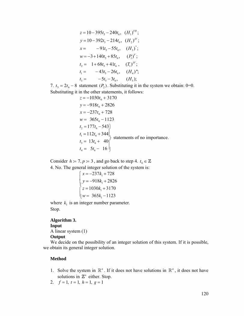
120
5 6 1
5 6 2'''
5 6 3
5 6 1
2 5 6 1
1 5 6 4
3 5 6
10 395 240 , ( ) ;
10 392 214 , ( ) ;
91 55 , ( ) ;
3 140 85 , ( ) ;
1 68 41 , ( ) ; 43 26 , ( ) ''; 5 3 ,
VII
IV
V
IV
z t t H
y t t H
x t t H
w t t P
t t t Tt t t Ht t t
= − −
= − −
= − −
= − + +
= + +
= − −= − − 5 ( );H
7. t5 = 2t6 − 8 statement (P2 ) . Substituting it in the system we obtain: 0=0. Substituting it in the other statements, it follows:
z = −1030t6 + 3170
y = −918t6 + 2826
x = −237t6 + 728
w = 365t6 − 1123
2 6
1 6
3 6
4 6
177 543112 344 13 40 5 16
t tt tt tt t
= − ⎫⎪= + ⎪⎬= + ⎪⎪= − ⎭
statements of no importance.
Consider h := 7, p := 3 , and go back to step 4. t6 ∈Z 4. No. The general integer solution of the system is:
1
1
1
1
237 728918 2826
1030 3170 365 1123
x ky kz kw k
= − +⎧⎪ = − +⎪⎨ = +⎪⎪ = −⎩
where k1 is an integer number parameter. Stop. Algorithm 3. Input A linear system (1) Output We decide on the possibility of an integer solution of this system. If it is possible, we obtain its general integer solution. Method
1. Solve the system in n . If it does not have solutions in n , it does not have solutions in Zn either. Stop.
2. f = 1, t = 1, h = 1, g = 1
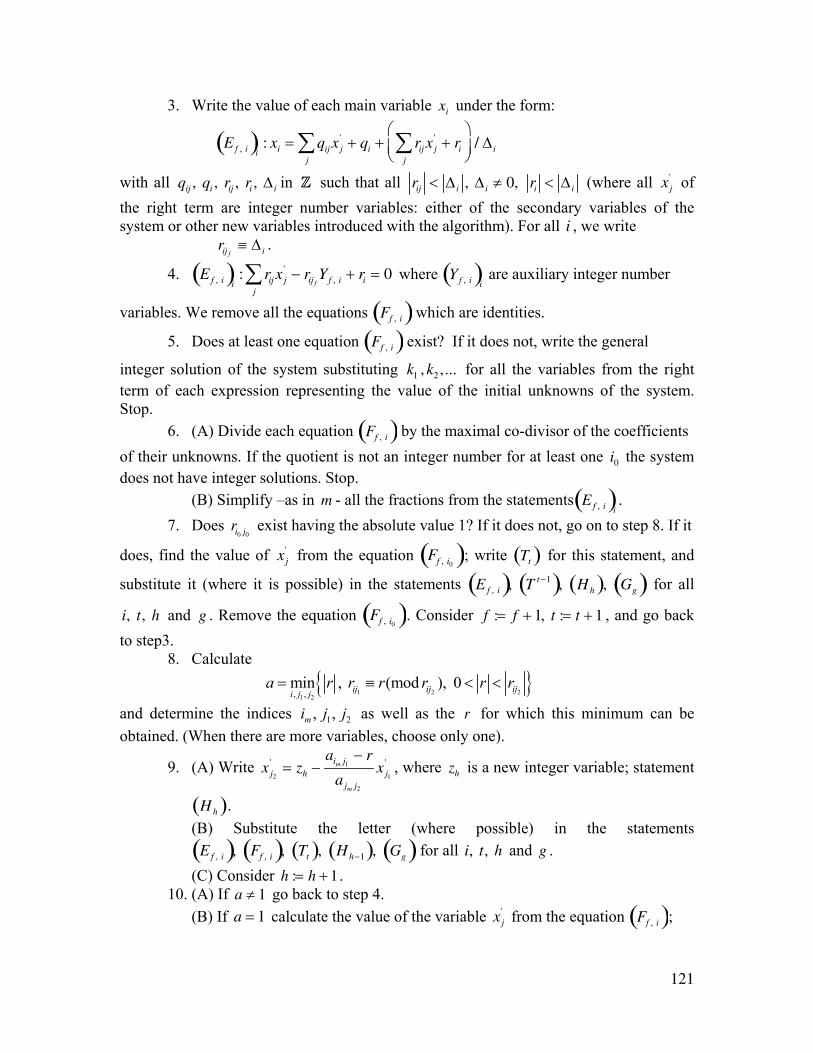
121
3. Write the value of each main variable xi under the form:
E f , i( )i: xi = qij
j∑ xj
' + qi + rijj
∑ xj' + ri
⎛
⎝⎜⎞
⎠⎟/ Δi
with all qij , qi , rij , ri , Δ i in Z such that all rij < Δ i , Δ i ≠ 0, ri < Δ i (where all xj' of
the right term are integer number variables: either of the secondary variables of the system or other new variables introduced with the algorithm). For all i , we write rij f
≡ Δ i .
4. E f , i( )i: rij
j∑ xj
' − rij fYf , i + ri = 0 where Yf , i( )
i are auxiliary integer number
variables. We remove all the equations Ff , i( ) which are identities.
5. Does at least one equation Ff , i( ) exist? If it does not, write the general
integer solution of the system substituting k1 , k2 ,... for all the variables from the right term of each expression representing the value of the initial unknowns of the system. Stop.
6. (A) Divide each equation Ff , i( ) by the maximal co-divisor of the coefficients of their unknowns. If the quotient is not an integer number for at least one i0 the system does not have integer solutions. Stop.
(B) Simplify –as in m - all the fractions from the statements E f , i( )i.
7. Does ri0 j0 exist having the absolute value 1? If it does not, go on to step 8. If it
does, find the value of xj' from the equation Ff , i0( ); write Tt( ) for this statement, and
substitute it (where it is possible) in the statements E f , i( ), T t −1( ), Hh( ), Gg( ) for all
i, t, h and g . Remove the equation Ff , i0( ). Consider f := f + 1, t := t + 1 , and go back to step3.
8. Calculate
{ }1 2 21 2, ,
min , (mod ), 0ij ij iji j ja r r r r r r= ≡ < <
and determine the indices 1 2, , mi j j as well as the r for which this minimum can be obtained. (When there are more variables, choose only one).
9. (A) Write x j2
' = zh −aim j1
− r
ajm j2
x j1
' , where zh is a new integer variable; statement
Hh( ). (B) Substitute the letter (where possible) in the statements
E f , i( ), Ff , i( ), Tt( ), Hh−1( ), Gg( ) for all i, t, h and g . (C) Consider h := h + 1 .
10. (A) If a ≠ 1 go back to step 4. (B) If a = 1 calculate the value of the variable xj
' from the equation Ff , i( );
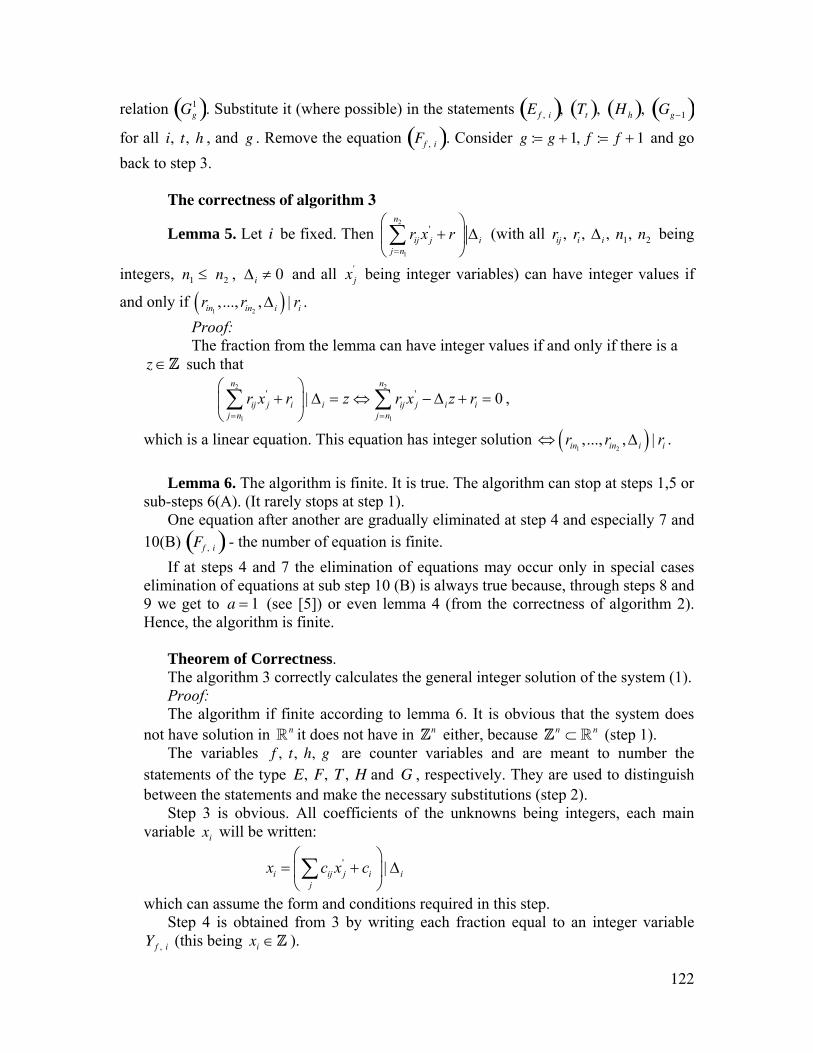
122
relation Gg1( ). Substitute it (where possible) in the statements E f , i( ), Tt( ), Hh( ), Gg−1( )
for all i, t, h , and g . Remove the equation Ff , i( ). Consider g := g + 1, f := f + 1 and go back to step 3.
The correctness of algorithm 3
Lemma 5. Let i be fixed. Then 2
1
'n
ij j ij n
r x r=
⎛ ⎞+ Δ⎜ ⎟
⎝ ⎠∑ (with all rij , ri , Δi , n1, n2 being
integers, n1 ≤ n2 , Δ i ≠ 0 and all xj' being integer variables) can have integer values if
and only if ( )1 2,..., , |in in i ir r rΔ .
Proof: The fraction from the lemma can have integer values if and only if there is a
z ∈Z such that
2 2
1 1
' '| 0n n
ij j i i ij j i ij n j n
r x r z r x z r= =
⎛ ⎞+ Δ = ⇔ − Δ + =⎜ ⎟
⎝ ⎠∑ ∑ ,
which is a linear equation. This equation has integer solution ⇔ ( )1 2,..., , |in in i ir r rΔ .
Lemma 6. The algorithm is finite. It is true. The algorithm can stop at steps 1,5 or sub-steps 6(A). (It rarely stops at step 1). One equation after another are gradually eliminated at step 4 and especially 7 and 10(B) Ff , i( ) - the number of equation is finite. If at steps 4 and 7 the elimination of equations may occur only in special cases elimination of equations at sub step 10 (B) is always true because, through steps 8 and 9 we get to a = 1 (see [5]) or even lemma 4 (from the correctness of algorithm 2). Hence, the algorithm is finite. Theorem of Correctness. The algorithm 3 correctly calculates the general integer solution of the system (1). Proof: The algorithm if finite according to lemma 6. It is obvious that the system does not have solution in n it does not have in Zn either, because n n⊂Z (step 1). The variables f , t, h, g are counter variables and are meant to number the statements of the type E, F, T , H and G , respectively. They are used to distinguish between the statements and make the necessary substitutions (step 2). Step 3 is obvious. All coefficients of the unknowns being integers, each main variable xi will be written:
' |i ij j i ij
x c x c⎛ ⎞
= + Δ⎜ ⎟⎝ ⎠∑
which can assume the form and conditions required in this step. Step 4 is obtained from 3 by writing each fraction equal to an integer variable Yf , i (this being xi ∈Z ).
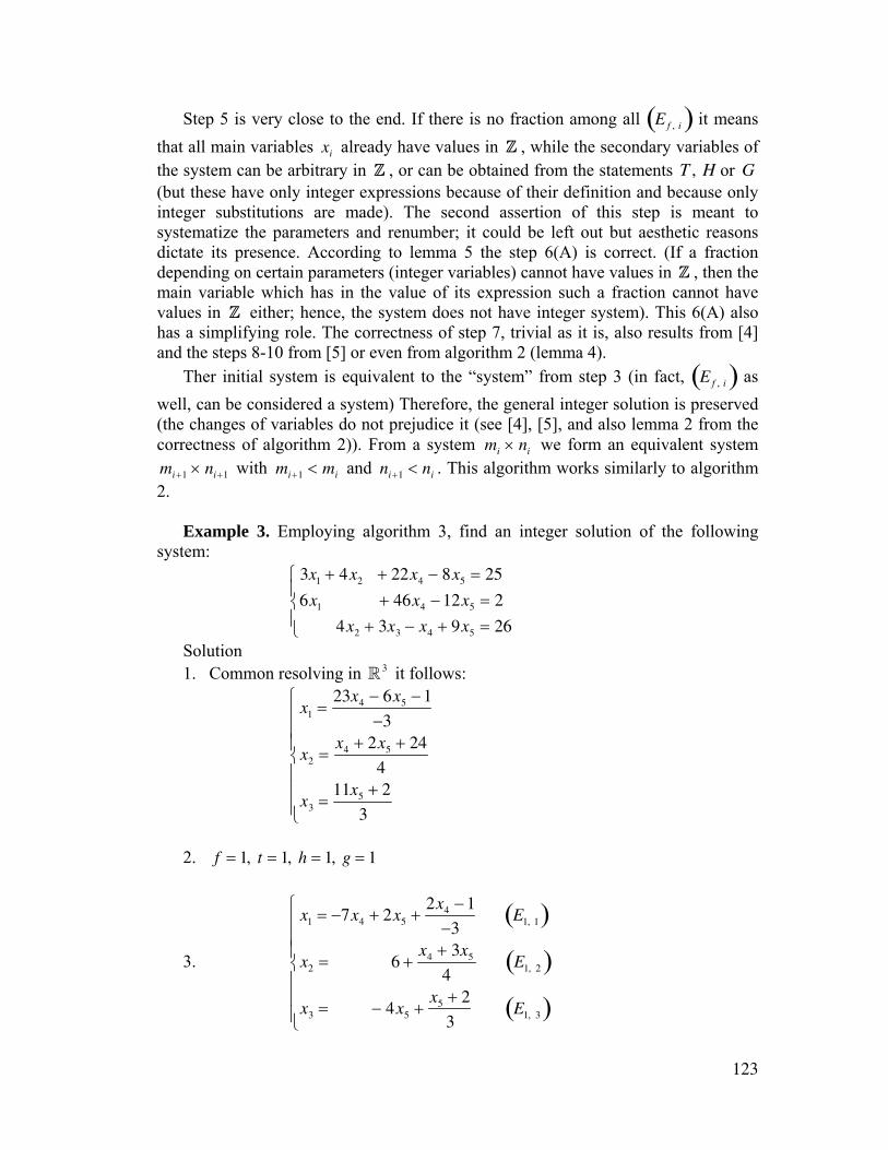
123
Step 5 is very close to the end. If there is no fraction among all E f , i( ) it means that all main variables xi already have values in Z , while the secondary variables of the system can be arbitrary in Z , or can be obtained from the statements T , H or G (but these have only integer expressions because of their definition and because only integer substitutions are made). The second assertion of this step is meant to systematize the parameters and renumber; it could be left out but aesthetic reasons dictate its presence. According to lemma 5 the step 6(A) is correct. (If a fraction depending on certain parameters (integer variables) cannot have values in Z , then the main variable which has in the value of its expression such a fraction cannot have values in Z either; hence, the system does not have integer system). This 6(A) also has a simplifying role. The correctness of step 7, trivial as it is, also results from [4] and the steps 8-10 from [5] or even from algorithm 2 (lemma 4). Ther initial system is equivalent to the “system” from step 3 (in fact, E f , i( ) as well, can be considered a system) Therefore, the general integer solution is preserved (the changes of variables do not prejudice it (see [4], [5], and also lemma 2 from the correctness of algorithm 2)). From a system mi × ni we form an equivalent system mi+1 × ni+1 with mi+1 < mi and ni+1 < ni . This algorithm works similarly to algorithm 2. Example 3. Employing algorithm 3, find an integer solution of the following system:
3x1 + 4x2 + 22x4 − 8x5 = 25
6x1 + 46x4 − 12x5 = 2
4x2 + 3x3 − x4 + 9x5 = 26
⎧
⎨⎪
⎩⎪
Solution 1. Common resolving in 3 it follows:
x1 =23x4 − 6x5 − 1
−3
x2 =x4 + 2x5 + 24
4
x3 =11x5 + 2
3
⎧
⎨
⎪⎪⎪
⎩
⎪⎪⎪
2. f = 1, t = 1, h = 1, g = 1
3.
x1 = −7x4 + 2x5 +2x4 − 1
−3 E1, 1( )
x2 = 6 +x4 + 3x5
4 E1, 2( )
x3 = − 4x5 +x5 + 2
3 E1, 3( )
⎧
⎨
⎪⎪⎪
⎩
⎪⎪⎪
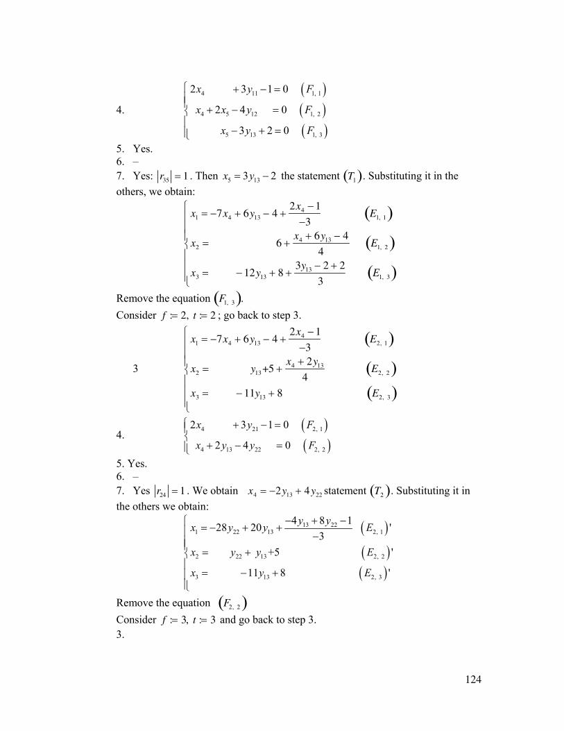
124
4.
( )( )( )
4 11 1, 1
4 5 12 1, 2
5 13 1, 3
2 3 1 0
2 4 0
3 2 0
x y F
x x y F
x y F
⎧ + − =⎪⎪ + − =⎨⎪
− + =⎪⎩
5. Yes. 6. – 7. Yes: r35 = 1 . Then 5 133 2x y= − the statement T1( ). Substituting it in the others, we obtain:
x1 = −7x4 + 6y13 − 4 +2x4 − 1
−3 E1, 1( )
x2 = 6 +x4 + 6y13 − 4
4 E1, 2( )
x3 = − 12y13 + 8 +3y13 − 2 + 2
3 E1, 3( )
⎧
⎨
⎪⎪⎪
⎩
⎪⎪⎪
Remove the equation F1, 3( ). Consider f := 2, t := 2 ; go back to step 3.
3
x1 = −7x4 + 6y13 − 4 +2x4 − 1
−3 E2, 1( )
x2 = y13+5 +x4 + 2y13
4 E2, 2( )
x3 = − 11y13 + 8 E2, 3( )
⎧
⎨
⎪⎪⎪
⎩
⎪⎪⎪
4. ( )( )
4 21 2, 1
4 13 22 2, 2
2 3 1 0
2 4 0
x y F
x y y F
⎧ + − =⎪⎨
+ − =⎪⎩
5. Yes. 6. – 7. Yes r24 = 1 . We obtain x4 = −2y13 + 4y22 statement T2( ). Substituting it in the others we obtain:
( )( )( )
13 221 22 13 2, 1
2 22 13 2, 2
3 13 2, 3
4 8 128 20 ' 3
+5 '
11 8 '
y yx y y E
x y y E
x y E
− + −⎧ = − + +⎪ −⎪⎪ = +⎨⎪
= − +⎪⎪⎩
Remove the equation F2, 2( ) Consider f := 3, t := 3 and go back to step 3.
3.
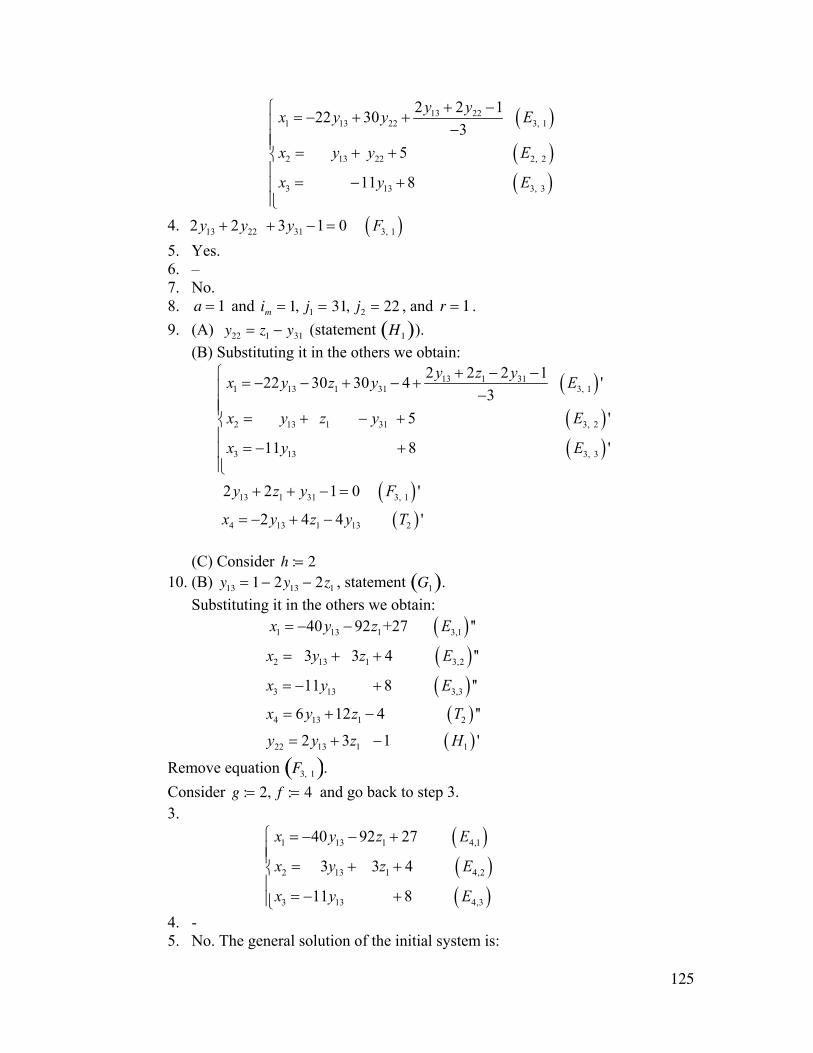
125
( )( )( )
13 221 13 22 3, 1
2 13 22 2, 2
3 13 3, 3
2 2 122 30 3
5
11 8
y yx y y E
x y y E
x y E
+ −⎧ = − + +⎪ −⎪⎪ = + +⎨⎪
= − +⎪⎪⎩
4. ( )13 22 31 3, 12 2 3 1 0 y y y F+ + − = 5. Yes. 6. – 7. No. 8. a = 1 and im = 1, j1 = 31, j2 = 22 , and r = 1 . 9. (A) y22 = z1 − y31 (statement H1( )).
(B) Substituting it in the others we obtain:
( )( )
13 1 311 13 1 31 3, 1
2 13 1 31 3, 2
3 13 3,
2 2 2 122 30 30 4 ' 3
5 '
11 8
y z yx y z y E
x y z y E
x y E
+ − −= − − + − +
−= + − +
= − + ( ) 3 '
⎧⎪⎪⎪⎨⎪⎪⎪⎩
( )( )
13 1 31 3, 1
4 13 1 13 2
2 2 1 0 '
2 4 4 '
y z y F
x y z y T
+ + − =
= − + −
(C) Consider h := 2
10. (B) y13 = 1 − 2y13 − 2z1 , statement G1( ). Substituting it in the others we obtain:
( )( )( )
( )( )
1 13 1 3,1
2 13 1 3,2
3 13 3,3
4 13 1 2
22 13 1 1
40 92 +27 ''
3 3 4 ''
11 8 ''
6 12 4 ''
2 3 1 '
x y z E
x y z E
x y E
x y z T
y y z H
= − −
= + +
= − +
= + −
= + −
Remove equation F3, 1( ). Consider g := 2, f := 4 and go back to step 3. 3.
( )( )( )
1 13 1 4,1
2 13 1 4,2
3 13 4,3
40 92 27
3 3 4
11 8
x y z E
x y z E
x y E
⎧ = − − +⎪⎪ = + +⎨⎪
= − +⎪⎩
4. - 5. No. The general solution of the initial system is:
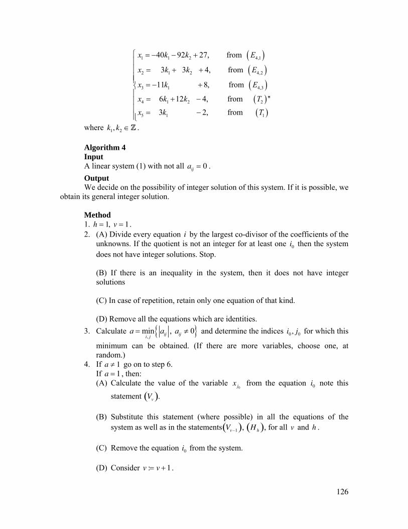
126
( )( )( )
( )
1 1 2 4,1
2 1 2 4,2
3 1 4,3
4 1 2 2
5 1
40 92 27, from
3 3 4, from
11 8, from
6 12 4, from ''
3 2, fro
x k k E
x k k E
x k E
x k k T
x k
= − − +
= + +
= − +
= + −
= − ( )1m T
⎧⎪⎪⎪⎪⎨⎪⎪⎪⎪⎩
where k1, k2 ∈Z . Algorithm 4 Input A linear system (1) with not all aij = 0 . Output
We decide on the possibility of integer solution of this system. If it is possible, we obtain its general integer solution.
Method 1. h = 1, v = 1 .
2. (A) Divide every equation i by the largest co-divisor of the coefficients of the unknowns. If the quotient is not an integer for at least one i0 then the system does not have integer solutions. Stop. (B) If there is an inequality in the system, then it does not have integer solutions (C) In case of repetition, retain only one equation of that kind. (D) Remove all the equations which are identities.
3. Calculate { },
min , 0ij iji ja a a= ≠ and determine the indices i0 , j0 for which this
minimum can be obtained. (If there are more variables, choose one, at random.)
4. If a ≠ 1 go on to step 6. If a = 1 , then: (A) Calculate the value of the variable x j0
from the equation i0 note this
statement Vv( ).
(B) Substitute this statement (where possible) in all the equations of the system as well as in the statements Vv−1( ), Hh( ), for all v and h .
(C) Remove the equation i0 from the system.
(D) Consider v := v + 1 .
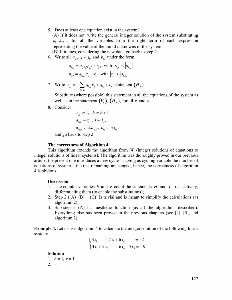
127
5. Does at least one equation exist in the system? (A) If it does not, write the general integer solution of the system substituting k1, k2 ,... for all the variables from the right term of each expression representing the value of the initial unknowns of the system.
(B) If it does, considering the new data, go back to step 2. 6. Write all ai0 j , j ≠ j0 and bi0
under the form :
ai0 j = ai0 j0qi0 j + ri0 j , with ri0 j < ai0 j .
0 0 0 0 0i j i j i ib a q r= + , with 0 0 0i i jr a< .
7. Write x j0= − qi0 j
j ≠ j0
∑ x j + qi0+ th , statement Hh( ).
Substitute (where possible) this statement in all the equations of the system as well as in the statement Vv( ), Hh( ), for all v and h .
8. Consider x j0
:= th , h := h + 1,
ai0 j := ri0 j , j ≠ j0 ,
ai0 j0:= ±ai0 j0
, bi0:= +ri0
,
and go back to step 2
The correctness of Algorithm 4 This algorithm extends the algorithm from [4] (integer solutions of equations to
integer solutions of linear systems). The algorithm was thoroughly proved in our previous article; the present one introduces a new cycle – having as cycling variable the number of equations of system – the rest remaining unchanged, hence, the correctness of algorithm 4 is obvious.
Discussion 1. The counter variables h and v count the statements H and V , respectively,
differentiating them (to enable the substitutions); 2. Step 2 ((A)+(B) + (C)) is trivial and is meant to simplify the calculations (as
algorithm 2); 3. Sub-step 5 (A) has aesthetic function (as all the algorithms described).
Everything else has been proved in the previous chapters (see [4], [5], and algorithm 2).
Example 4. Let us use algorithm 4 to calculate the integer solution of the following linear system:
1 3 4
1 2 4 5
3 7 6 24 3 6 5 19x x xx x x x
− + = −⎧⎨ + + − =⎩
Solution 1. h = 1, v = 1
2. –
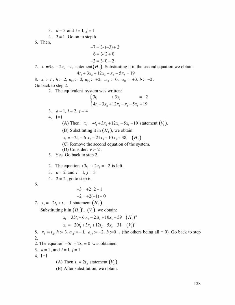
128
3. a = 3 and i = 1, j = 1 4. 3 ≠ 1 . Go on to step 6.
6. Then, −7 = 3 ⋅ (−3) + 2
6 = 3 ⋅ 2 + 0
−2 = 3 ⋅ 0 − 2
7. x1 =3x3 − 2x4 + t1 statement H1( ). Substituting it in the second equation we obtain: 4t1 + 3x2 + 12x3 − x4 − 5x5 = 19
8. x1 := t1, h := 2, a12 := 0, a13 := +2, a14 := 0, a11 := +3, b := −2 . Go back to step 2.
2. The equivalent system was written: 1 3
1 2 3 4 5
3 3 24 3 12 5 19t xt x x x x
+ = −⎧⎨ + + − − =⎩
3. a = 1, i = 2, j = 4 4. 1=1
(A) Then: 4 1 2 3 54 3 12 5 19x t x x x= + + − − statement V1( ). (B) Substituting it in H1( ), we obtain: x1 = −7t1 − 6 x2 − 21x3 + 10x5 + 38, H1( ) (C) Remove the second equation of the system. (D) Consider: v := 2 .
5. Yes. Go back to step 2.
2. The equation 1 33 2 2t x+ + = − is left. 3. a = 2 and i = 1, j = 3 4. 2 ≠ 2 , go to step 6.
6. +3 = +2 ⋅ 2 − 1
−2 = +2(−1) + 0
7. x3 = −2t1 + t2 − 1 statement H 2( ). Substituting it in H1( )' , V1( ), we obtain:
( )( )
1 1 2 2 5 1
4 1 2 2 5 1
35 6 21 10 59 ''
20 3 12 5 31 '
x t x t x H
x t x t x V
= − − + +
= − + + − −
8. x3 := t2 , h := 3, a11:= − 1, a13 := +2, b1:=0 , (the others being all = 0). Go back to step 2. 2. The equation −5t1 + 2t2 = 0 was obtained. 3. a = 1 , and i = 1, j = 1 4. 1=1
(A) Then t1 = 2t2 statement V2( ). (B) After substitution, we obtain:
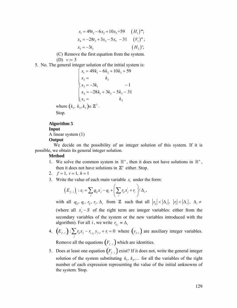
129
( )( )
( )
1 2 2 5 1
4 2 2 5 1
3 2 2
49 6 10 +59 ''';
28 3 5 31 '' ;
3 ';
x t x x H
x t x x V
x t H
= − +
= − + − −
= −
(C) Remove the first equation from the system. (D) v := 3
5. No. The general integer solution of the initial system is:
x1 = 49k1 − 6k2 + 10k3 + 59
x2 = k2
x3 = −3k1 − 1
x4 = −28k1 + 3k2 − 5k3 − 31
x5 = k3
⎧
⎨
⎪⎪⎪
⎩
⎪⎪⎪
where k1, k2 , k3( )∈Z3 . Stop.
Algorithm 5
Input A linear system (1) Output We decide on the possibility of an integer solution of this system. If it is
possible, we obtain its general integer solution. Method 1. We solve the common system in n , then it does not have solutions in n ,
then it does not have solutions in Zn either. Stop. 2. f = 1, v = 1, h = 1 3. Write the value of each main variable xi under the form:
( ) ' ', : /f i i ij j i ij j i ii
j j
E x q x q r x r⎛ ⎞
= − + + Δ⎜ ⎟⎝ ⎠
∑ ∑ ,
with all qij , qi , rij , ri , Δi from Z such that all rij < Δ i , ri < Δ i , Δ i ≠
(where all 'jx S− of the right term are integer variables: either from the
secondary variables of the system or the new variables introduced with the algorithm). For all i , we write rij f
≡ Δ i
4. Ef , i( )i: rij
j∑ x j − ri, j f
y f ,i + ri = 0 where yf ,i( ) are auxiliary integer variables.
Remove all the equations Ff , i( ) which are identities.
5. Does at least one equation Ff , i( ) exist? If it does not, write the general integer solution of the system substituting k1, k2 ,... for all the variables of the right number of each expression representing the value of the initial unknowns of the system. Stop.
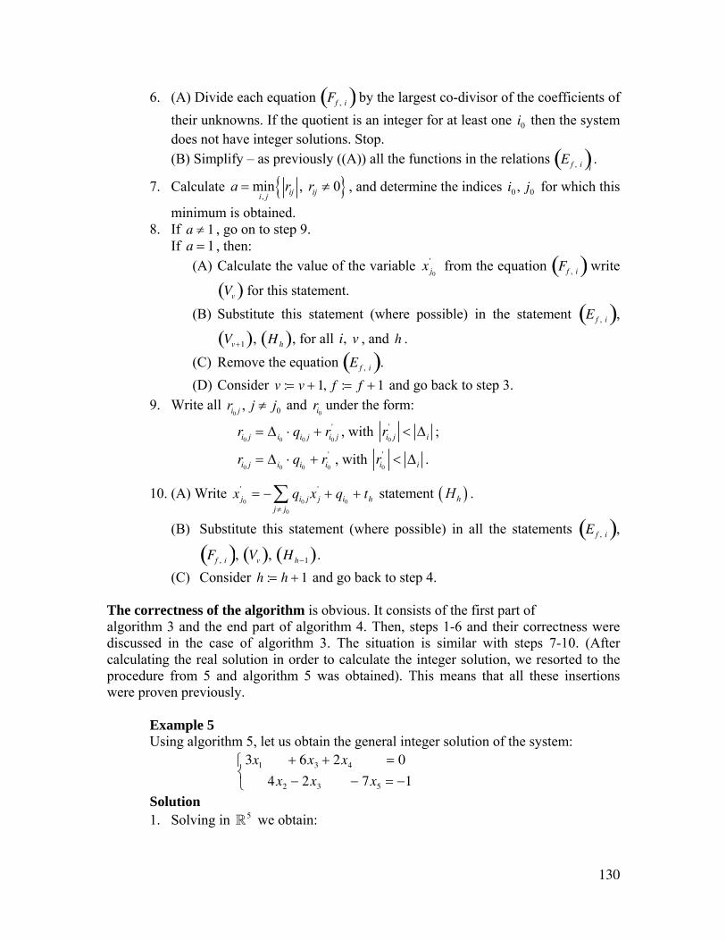
130
6. (A) Divide each equation Ff , i( ) by the largest co-divisor of the coefficients of their unknowns. If the quotient is an integer for at least one i0 then the system does not have integer solutions. Stop. (B) Simplify – as previously ((A)) all the functions in the relations E f , i( )
i.
7. Calculate { },
min , 0ij iji ja r r= ≠ , and determine the indices i0 , j0 for which this
minimum is obtained. 8. If a ≠ 1 , go on to step 9.
If a = 1 , then: (A) Calculate the value of the variable x j0
' from the equation Ff , i( ) write
Vv( ) for this statement.
(B) Substitute this statement (where possible) in the statement E f , i( ),
Vv+1( ), Hh( ), for all i, v , and h .
(C) Remove the equation E f , i( ). (D) Consider v := v + 1, f := f + 1 and go back to step 3.
9. Write all 0 0, i jr j j≠ and ri0
under the form:
ri0 j = Δi0⋅ qi0 j + ri0 j
' , with ri0 j' < Δi ;
ri0 j = Δi0⋅ qi0
+ ri0
' , with ri0
' < Δi .
10. (A) Write x j0
' = − qi0 jj ≠ j0
∑ x j' + qi0
+ th statement ( )hH .
(B) Substitute this statement (where possible) in all the statements E f , i( ),
Ff , i( ), Vv( ), Hh−1( ). (C) Consider h := h + 1 and go back to step 4.
The correctness of the algorithm is obvious. It consists of the first part of algorithm 3 and the end part of algorithm 4. Then, steps 1-6 and their correctness were discussed in the case of algorithm 3. The situation is similar with steps 7-10. (After calculating the real solution in order to calculate the integer solution, we resorted to the procedure from 5 and algorithm 5 was obtained). This means that all these insertions were proven previously. Example 5 Using algorithm 5, let us obtain the general integer solution of the system:
3x1 + 6x3 + 2x4 = 0
4x2 − 2x3 − 7x5 = −1
⎧⎨⎩
Solution 1. Solving in 5 we obtain:
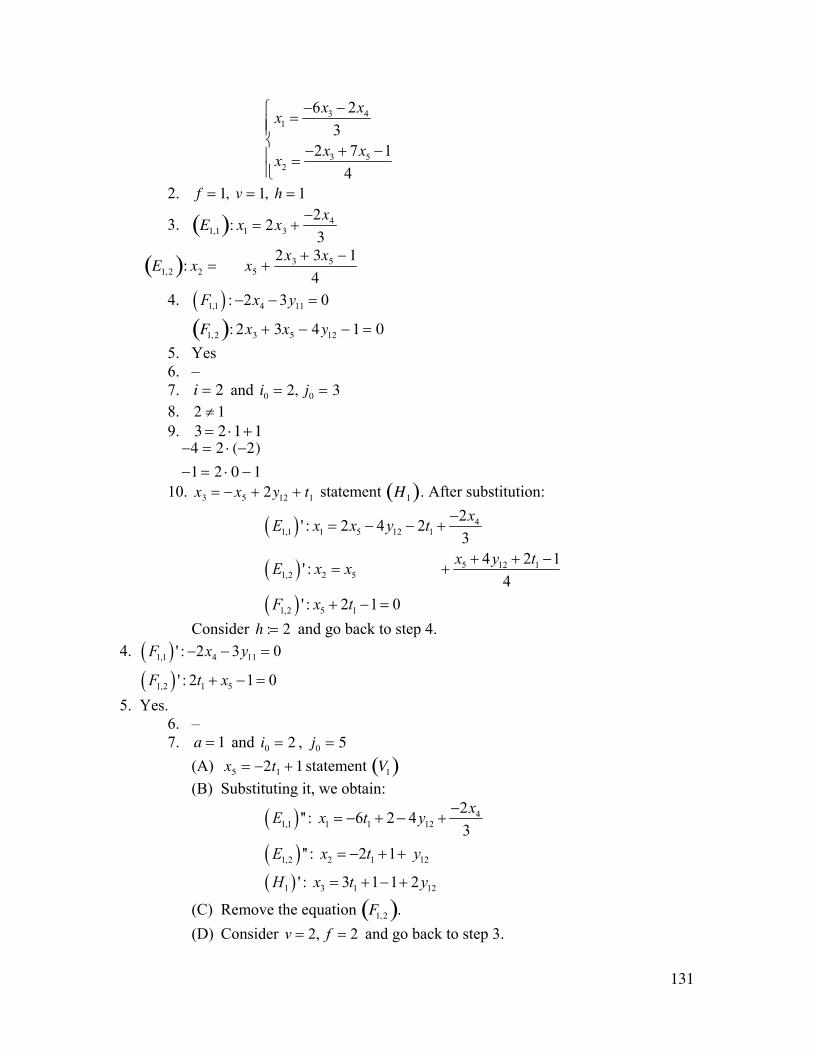
131
3 41
3 52
6 23
2 7 14
x xx
x xx
− −⎧ =⎪⎪⎨ − + −⎪ =⎪⎩
2. f = 1, v = 1, h = 1
3. E1,1( ): x1 = 2x3 +−2x4
3
E1,2( ): x2 = x5 +2x3 + 3x5 − 1
4
4. ( )1,1 4 11: 2 3 0F x y− − =
F1,2( ): 2x3 + 3x5 − 4y12 − 1 = 0 5. Yes 6. – 7. i = 2 and i0 = 2, j0 = 3 8. 2 ≠ 1 9. 3 = 2 ⋅1+ 1
−4 = 2 ⋅ (−2)
−1 = 2 ⋅ 0 − 1
10. x3 = −x5 + 2y12 + t1 statement H1( ). After substitution:
( )
( )( )
41,1 1 5 12 1
5 12 11,2 2 5
1,2 5 1
2' : 2 4 23
4 2 1' : 4
' : 2 1 0
xE x x y t
x y tE x x
F x t
−= − − +
+ + −= +
+ − =
Consider h := 2 and go back to step 4. 4. ( )1,1 4 11' : 2 3 0F x y− − =
( )1,2 1 5' : 2 1 0F t x+ − = 5. Yes.
6. – 7. a = 1 and i0 = 2 , j0 = 5
(A) x5 = −2t1 + 1 statement V1( ) (B) Substituting it, we obtain:
( )( )( )
41,1 1 1 12
1,2 2 1 12
1 3 1 12
2'' : 6 2 43
'' : 2 1
' : 3 1 1 2
xE x t y
E x t y
H x t y
−= − + − +
= − + +
= + − +
(C) Remove the equation F1,2( ). (D) Consider 2, 2v f= = and go back to step 3.
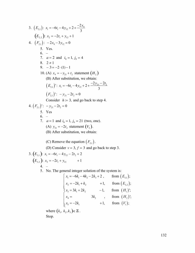
132
3. ( ) 42,1 1 1 12
2: 6 4 23xE x t y −
= − − + +
E2,2( ): x2 = −2t1 + y12 + 1
4. ( )2,1 4 12: 2 3 0F x y− − = 5. Yes. 6. – 7. a = 2 and i0 = 1, j0 = 4 8. 2 ≠ 1 9. − 3 = −2 ⋅ (1) − 1 10. (A) x4 = −y21 + t2 statement H 2( )
(B) After substitution, we obtain:
( )( )
21 22,1 1 1 12
2,1 21 2
2 2' : 6 4 23
' : 2 0
y tE x t y
F y t
− −= − − + +
− − =
Consider h := 3, and go back to step 4. 4. ( )2,1 21 2' : 2 0F y t− − =
5. Yes 6. – 7. a = 1 and i0 = 1, j0 = 21 (two, one).
(A) y21 = −2t2 statement V2( ). (B) After substitution, we obtain: (C) Remove the equation ( )2,1F . (D) Consider v = 3, f = 3 and go back to step 3.
3. E3,1( ): x1 = −6t1 − 4y12 − 2t2 + 2
E3,2( ): x2 = −2t1 + y12 + 1 4. – 5. No. The general integer solution of the system is:
( )( )( )( )
1 1 2 3 3,1
2 1 2 3,2
3 1 2 1
4 3 2
5 1
6 4 2 2 , from ;
2 1, from ;
3 2 1, from ';
3 , from ';
2
x k k k E
x k k E
x k k H
x k H
x k
= − − − +
= − + +
= + −
=
= − ( )1 1, from ; V
⎧⎪⎪⎪⎪⎨⎪⎪⎪ +⎪⎩
where k1, k2 ,k3( )∈Z . Stop.
133
Note 1. Algorithm 3, 4, and 5 can be applied in the calculation of the integer solution of a linear equation. Note 2. The algorithms, because of their form, are easily adapted to a computer program. Note 3. It is up to the reader to decide on which algorithm to use. Good luck! REFERENCES
[1] Smarandache, Florentin – Rezolvarea ecuaţiilor şi a sistemelor de ecuaţii liniare în numere întregi - diploma paper, University of Craiova, 1979.
[2] Smarandache, Florentin – Généralisations et généralités - Edition Nouvelle, Fès (Maroc), 1984.
[3] Smarandache, Florentin – Problems avec et sans .. problèmes! Somipress, Fès (Maroc), 1983.
[4] Smarandache, Florentin – General solution proprieties in whole numbers for linear equations – Bul. Univ. Braşov, Series C, Mathematics, vol. XXIV, pp. 37-39, 1982.
[5] Smarandache, Florentin – Baze de soluţii pentru congruenţe lineare – Bul. Univ. Braşov, Series C, Mathematics, vol. XXII, pp. 25-31, 1980, re-published in Buletinul Ştiinţific şi Tehnic al Institutului Politehnic “Traian Vuia”, Timişoara, Series Mathematics-Physics, tome 26 (40) fascicle 2, pp. 13-16, 1981, reviewed in Mathematical Rev. (USA): 83e:10006.
[6] Smarandache, Florentin – O generalizare a teoremei lui Euler referitoare la congruenţe – Bul. Univ. Braşov, series C, mathematics, vol. XXII, pp. 07-12, reviewed in Mathematical Reviews (USA): 84j:10006.
[7] Creangă, I., Cazacu, C., Mihuţ, P., Opaiţ, Gh., Corina Reischer – Introcucere în teoria numerelor - Editura Didactică şi Pedagogică, Bucharest, 1965.
[8] Cucurezeanu, Ion – Probleme de aritmetică şi teoria numerelor, Editura Tehnică, Buharest, 1976.
[9] Ghelfond, A. O. – Rezolvarea ecuaţiilor în numere întregi - translation from Russian, Editura Tehnică, Bucharest, 1954.
[10] Golstein, E., Youndin, D. – Problemes particuliers de la programmation lineaire - Edition Mir, Moscou, Traduit de russe, 1973.
[11] Ion, D. Ion, Niţă, C. – Elemente de aritmetică cu aplicaţii în tehnici de calcul, Editura Tehnică, Bucharest, 1978.
[12] Ion, D. Ion, Radu, K. – Algebra - Editura Didactică şi Pedagogică, Bucharest 1970.
[13] Mordell, L. – Two papers on number theory - Veb Deutscher Verlag der Wissenschafen, Berlin, 1972.
[14] Popovici, C. P. – Aritmetica şi teoria numerelor - Editura Didactică şi Pedagogică, Bucharest, 1963.
134
[15] Popovici, C. P. – Logica şi teoria numerelor - Editura Didactică şi Pedagogică, Bucharest, 1970.
[16] Popovici, C. P. – Teoria numerelor – lecture course, Editura Didactică şi Pedagogică, Bucharest, 1973.
[17] Rusu, E – Aritmetica si teoria numerelor - Editura Didactică şi Pedagogică, Bucharest, 1963.
[18] Rusu, E. – Bazele teoriei numerelor - Editura Tehincă, Bucharest, 1953. [19] Sierpinski, W. – Ce ştim şi ce nu ştim despre numerele prime – Editura.
Ştiinţifică, Bucharest, 1966. [20] Sierpinski, W. – 250 problemes de theorie elementaires des nombres -
Classiques Hachette, Paris, 1972.
[Partialy published in “Bulet. Univ. Braşov”, series C, Vol. XXIV, pp. 37-9, 1982, under the title: “General integer solution properties for linear equations”.]
135
A METHOD TO GENERALIZE BY RECURRENCE OF
SOME KNOWN RESULTS
A great number of articles widen known results, and this is due to a simple procedure, of which it is good to say a few words:
Let say that one generalizes a known mathematical proposition P(a) , where a is a constant, to the proposition P(n) , where n is a variable which belongs to subset of N . To prove that P is true for n by recurrence means the following: the first step is banal, since it is about the known result P(a) (and thus it was already verified before by other mathematicians!). To pass from P(n) to P(n + 1) , one uses too P(a) : therefore one widens a proposition by using the proposition itself, in other words the found generalization will be paradoxically proved with the help of the particular case from which one started! (e. g. the generalizations of Hölder, Minkovski, Tchebychev, Euler).
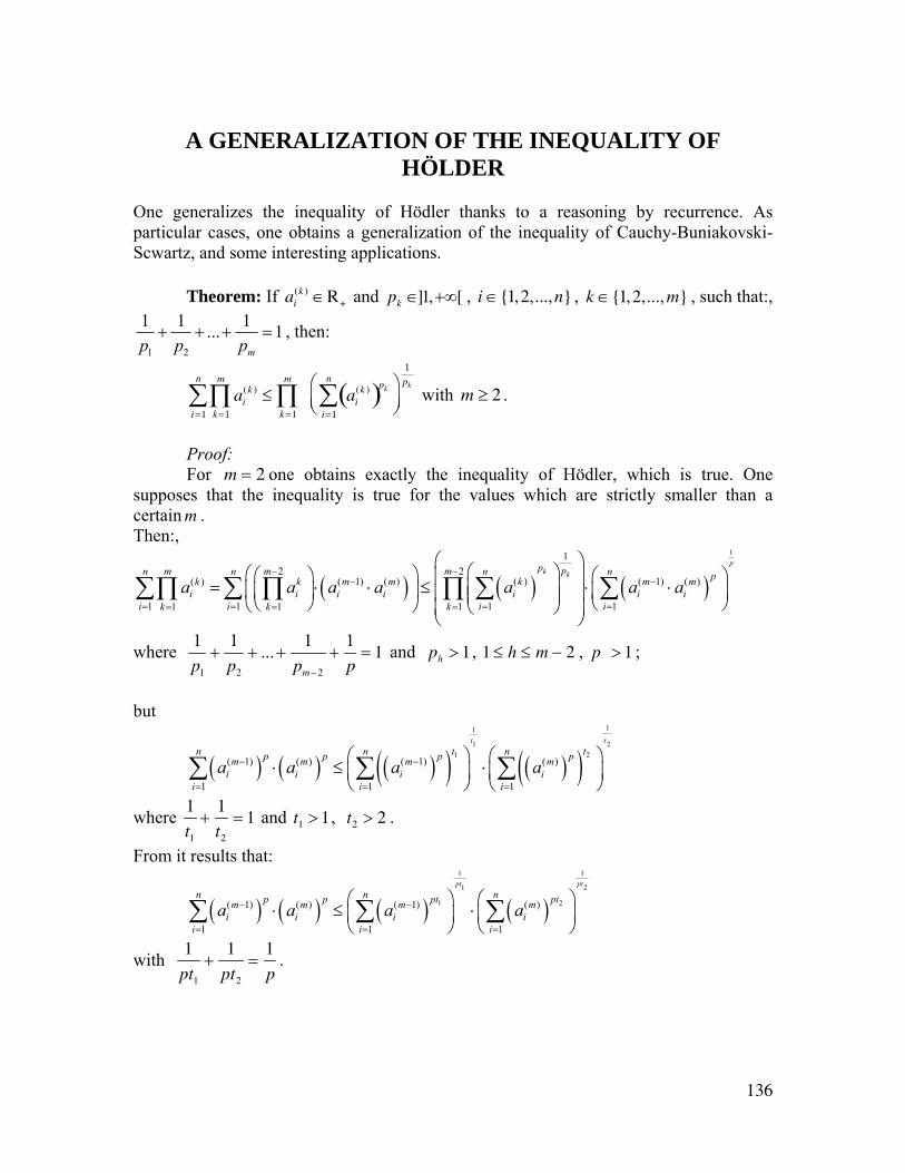
136
A GENERALIZATION OF THE INEQUALITY OF HÖLDER
One generalizes the inequality of Hödler thanks to a reasoning by recurrence. As particular cases, one obtains a generalization of the inequality of Cauchy-Buniakovski-Scwartz, and some interesting applications. Theorem: If ai
(k ) ∈R+ and pk ∈]1,+∞[ , i ∈{1,2,...,n} , k ∈{1,2,..., m} , such that:,
1 2
1 1 1... 1mp p p
+ + + = , then:
ai(k )
k =1
m
∏i=1
n
∑ ≤k =1
m
∏ ai(k )( )pk
i=1
n
∑⎛⎝⎜
⎞⎠⎟
1
pk
with m ≥ 2 .
Proof: For m = 2 one obtains exactly the inequality of Hödler, which is true. One
supposes that the inequality is true for the values which are strictly smaller than a certain m . Then:,
( ) ( ) ( )11
2 2( ) ( 1) ( ) ( ) ( 1) ( )
1 1 1 11 1 1
pk k
p pm m mn n n n pk k m m k m mi i i i i i i
i i i ik k k
a a a a a a a− −
− −
= = = == = =
⎛ ⎞⎛ ⎞⎛ ⎞⎛ ⎞ ⎛ ⎞⎜ ⎟= ⋅ ⋅ ≤ ⋅ ⋅⎜ ⎟⎜ ⎟⎜ ⎟ ⎜ ⎟⎜ ⎟⎜ ⎟ ⎝ ⎠⎝ ⎠⎝ ⎠ ⎝ ⎠⎜ ⎟
⎝ ⎠
∑ ∑ ∑ ∑∏ ∏ ∏
where 1
p1
+1
p2
+ ... +1
pm− 2
+1
p= 1 and ph > 1 , 1 ≤ h ≤ m − 2 , p > 1 ;
but
( ) ( ) ( )( ) ( )( )11
1 21 2
( 1) ( ) ( 1) ( )
1 1 1
t tt tn n np p p pm m m m
i i i ii i i
a a a a− −
= = =
⎛ ⎞ ⎛ ⎞⋅ ≤ ⋅⎜ ⎟ ⎜ ⎟
⎝ ⎠ ⎝ ⎠∑ ∑ ∑
where 1
t1
+1
t2
= 1 and t1 > 1 , t2 > 2 .
From it results that:
( ) ( ) ( ) ( )1 1
1 2
1 2( 1) ( ) ( 1) ( )
1 1 1
pt ptn n np p pt ptm m m m
i i i ii i i
a a a a− −
= = =
⎛ ⎞ ⎛ ⎞⋅ ≤ ⋅⎜ ⎟ ⎜ ⎟
⎝ ⎠ ⎝ ⎠∑ ∑ ∑
with 1
pt1
+1
pt2
=1
p.
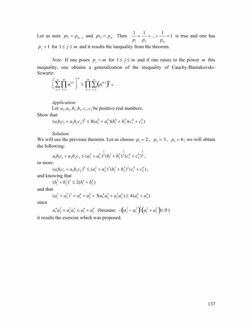
137
Let us note pt1 = pm−1 and pt2 = pm . Then 1 2
1 1 1... 1mp p p
+ + + = is true and one has
pj > 1 for 1 ≤ j ≤ m and it results the inequality from the theorem.
Note: If one poses pj = m for 1 ≤ j ≤ m and if one raises to the power m this inequality, one obtains a generalization of the inequality of Cauchy-Buniakovski-Scwartz:
ai(k )
k =1
m
∏i=1
n
∑⎛⎝⎜
⎞⎠⎟
m
≤ ai(k )( )m
i=1
n
∑k =1
m
∏ .
Application: Let a1,a2 ,b1,b2 ,c1,c2 be positive real numbers.
Show that: (a1b1c1 + a2b2c2 )6 ≤ 8(a1
6 + a26 )(b1
6 + b26 )(c1
6 + c26 )
Solution: We will use the previous theorem. Let us choose p1 = 2 , p2 = 3 , p3 = 6 ; we will obtain the following:
a1b1c1 + a2b2c2 ≤ (a12 + a2
2 )1
2 (b13 + b2
3)1
3 (c16 + c2
6 )1
6 , or more:
(a1b1c1 + a2b2c2 )6 ≤ (a12 + a2
2 )3(b13 + b2
3 )2 (c16 + c2
6 ) , and knowing that
3 3 2 6 61 2 1 2( ) 2( )b b b b+ ≤ +
and that (a1
2 + a22 )3 = a1
6 + a26 + 3(a1
4a22 + a1
2a24 ) ≤ 4(a1
6 + a26 )
since a1
4a22 + a1
2a24 ≤ a1
6 + a26 (because: − a2
2 − a12( )2
a12 + a2
2( )≤ 0 ) it results the exercise which was proposed.

138
A GENERALIZATION OF THE INEQUALITY OF MINKOWSKI
Theorem : If p is a real number ≥ 1 and ( )k
ia ∈R+ with i ∈{1,2,...,n} and k ∈{1,2,..., m} , then:
1 1/
( ) ( )
1 1 1 1
p pp pn m m nk k
i ii k k i
a a= = = =
⎛ ⎞ ⎛ ⎞⎛ ⎞ ⎛ ⎞≤⎜ ⎟ ⎜ ⎟⎜ ⎟ ⎜ ⎟⎜ ⎟ ⎜ ⎟⎝ ⎠ ⎝ ⎠⎝ ⎠ ⎝ ⎠
∑ ∑ ∑ ∑
Demonstration by recurrence on m∈N*. First of all one shows that:
ai(1)( )p
i=1
n
∑⎛⎝⎜
⎞⎠⎟
1 p
≤ ai(1)( )p
i=1
n
∑⎛⎝⎜
⎞⎠⎟
1/ p
, which is obvious, and proves that the inequality
is true for m = 1 . (The case m = 2 precisely constitutes the inequality of Minkowski, which is naturally true!).
Let us suppose that the inequality is true for all the values less or equal to m
1 111 1( ) (1) ( )
1 1 1 1 2
p
p pp p pn m n n mk k
i i ii k i i k
a a a+ +
= = = = =
⎛ ⎞ ⎛ ⎞⎛ ⎞ ⎛ ⎞ ⎛ ⎞≤ + ≤⎜ ⎟ ⎜ ⎟⎜ ⎟ ⎜ ⎟ ⎜ ⎟⎜ ⎟ ⎜ ⎟⎝ ⎠ ⎝ ⎠ ⎝ ⎠⎝ ⎠ ⎝ ⎠
∑ ∑ ∑ ∑ ∑
≤ ai(1)( )p
i=1
n
∑⎛⎝⎜
⎞⎠⎟
1 p
+ ai(k )
i=1
n
∑⎛⎝⎜
⎞⎠⎟
p
k =2
m+1
∑⎛
⎝⎜
⎞
⎠⎟
1 p
and this last sum is ai(k )
i=1
n
∑⎛⎝⎜
⎞⎠⎟
p
k =1
m+1
∑⎛
⎝⎜
⎞
⎠⎟
1 p
therefore the inequality is true for the level m + 1 .
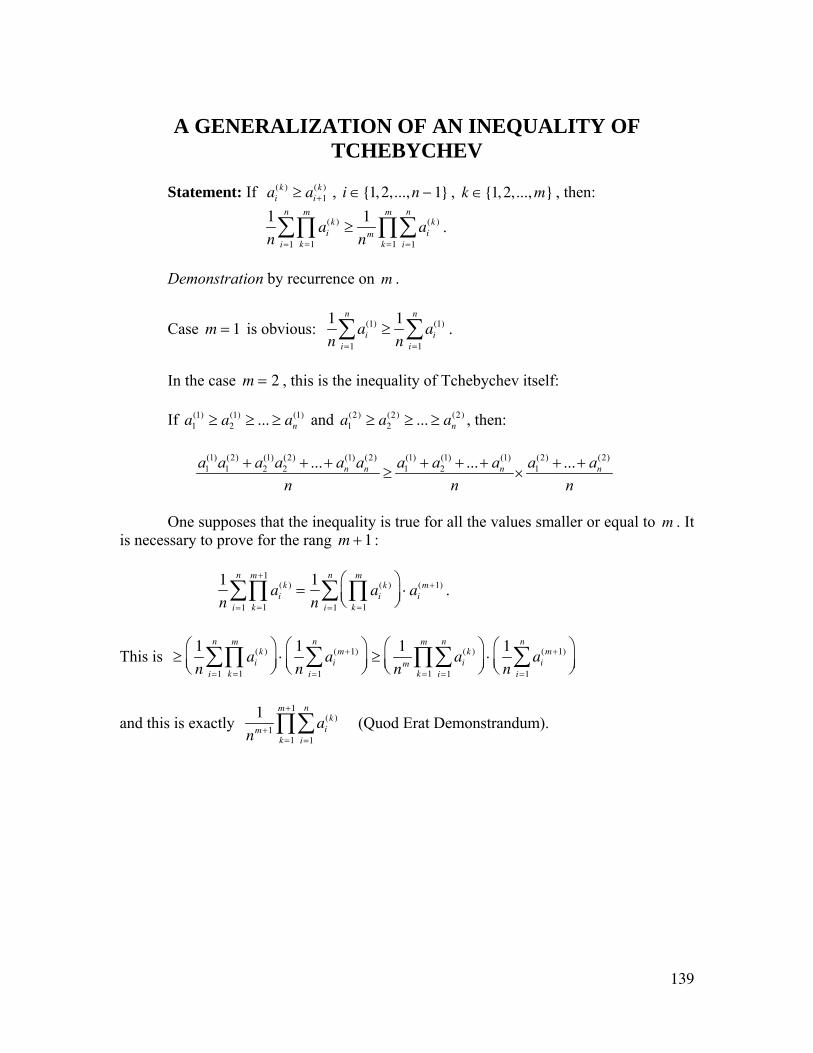
139
A GENERALIZATION OF AN INEQUALITY OF TCHEBYCHEV
Statement: If ai
(k ) ≥ ai+1(k ) , i ∈{1,2,...,n − 1} , k ∈{1,2,..., m} , then:
1
nai
(k )
k =1
m
∏i=1
n
∑ ≥1
nmai
(k )
i=1
n
∑k =1
m
∏ .
Demonstration by recurrence on m .
Case m = 1 is obvious: 1
nai
(1)
i=1
n
∑ ≥1
nai
(1)
i=1
n
∑ .
In the case m = 2 , this is the inequality of Tchebychev itself: If a1
(1) ≥ a2(1) ≥ ... ≥ an
(1) and a1(2) ≥ a2
(2) ≥ ... ≥ an(2) , then:
(1) (2) (1) (2) (1) (2) (1) (1) (1) (2) (2)1 1 2 2 1 2 1... ... ...n n n na a a a a a a a a a a
n n n+ + + + + + + +
≥ ×
One supposes that the inequality is true for all the values smaller or equal to m . It
is necessary to prove for the rang m + 1 :
1
nai
(k )
k =1
m+1
∏i=1
n
∑ =1
nai
(k )
k =1
m
∏⎛⎝⎜
⎞⎠⎟i=1
n
∑ ⋅ ai(m+1) .
This is ≥1
nai
(k )
k =1
m
∏i=1
n
∑⎛⎝⎜
⎞⎠⎟
⋅1
nai
(m+1)
i=1
n
∑⎛⎝⎜
⎞⎠⎟
≥1
nmai
(k )
i=1
n
∑k =1
m
∏⎛⎝⎜
⎞⎠⎟
⋅1
nai
(m+1)
i=1
n
∑⎛⎝⎜
⎞⎠⎟
and this is exactly 1
nm+1 ai(k )
i=1
n
∑k =1
m+1
∏ (Quod Erat Demonstrandum).
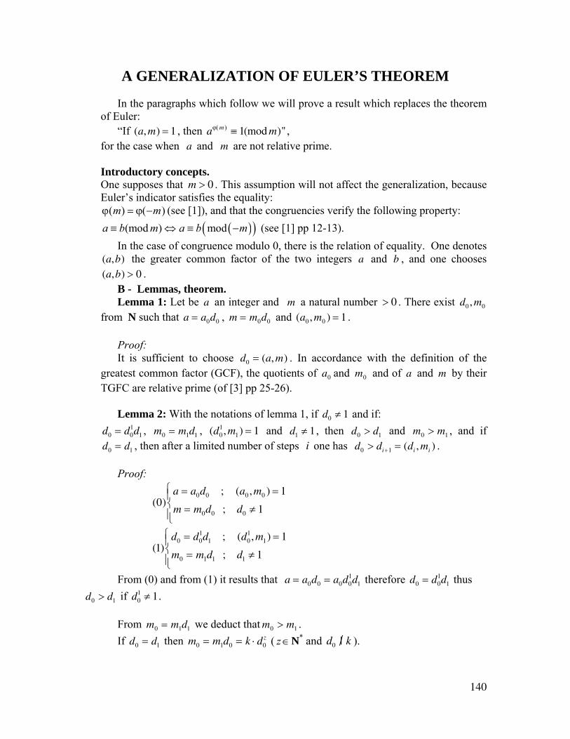
140
A GENERALIZATION OF EULER’S THEOREM In the paragraphs which follow we will prove a result which replaces the theorem of Euler: “If (a,m) = 1 , then aϕ(m ) ≡ 1(mod m)" , for the case when a and m are not relative prime. Introductory concepts. One supposes that m > 0 . This assumption will not affect the generalization, because Euler’s indicator satisfies the equality:
( )m mϕ = ϕ(− ) (see [1]), and that the congruencies verify the following property: ( )( )(mod ) moda b m a b m≡ ⇔ ≡ − (see [1] pp 12-13).
In the case of congruence modulo 0, there is the relation of equality. One denotes (a,b) the greater common factor of the two integers a and b , and one chooses (a,b) > 0 . B - Lemmas, theorem. Lemma 1: Let be a an integer and m a natural number > 0 . There exist d0 , m0 from N such that a = a0d0 , m = m0d0 and (a0 , m0 ) = 1 . Proof: It is sufficient to choose d0 = (a, m) . In accordance with the definition of the greatest common factor (GCF), the quotients of a0 and m0 and of a and m by their TGFC are relative prime (of [3] pp 25-26). Lemma 2: With the notations of lemma 1, if d0 ≠ 1 and if: d0 = d0
1d1 , m0 = m1d1 , (d01, m1) = 1 and d1 ≠ 1 , then d0 > d1 and m0 > m1 , and if
d0 = d1 , then after a limited number of steps i one has d0 > di+1 = (di , mi ) . Proof:
(0)a = a0d0 ; (a0 , m0 ) = 1
m = m0d0 ; d0 ≠ 1
⎧⎨⎪
⎩⎪
(1)d0 = d0
1d1 ; (d01, m1) = 1
m0 = m1d1 ; d1 ≠ 1
⎧⎨⎪
⎩⎪
From (0) and from (1) it results that a = a0d0 = a0d01d1 therefore d0 = d0
1d1 thus d0 > d1 if d0
1 ≠ 1.
From m0 = m1d1 we deduct that m0 > m1 . If d0 = d1 then m0 = m1d0 = k ⋅ d0
z ( z ∈N* and d0 | k ).
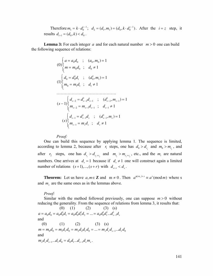
141
Therefore m1 = k ⋅ d0z−1 ; d2 = (d1, m1) = (d0 , k ⋅ d0
z−1) . After the i = z step, it results di+1 = (d0 ,k) < d0 .
Lemma 3: For each integer a and for each natural number m > 0 one can build
the following sequence of relations:
(0)a = a0d0 ; (a0 , m0 ) = 1
m = m0d0 ; d0 ≠ 1
⎧⎨⎪
⎩⎪
(1)d0 = d0
1d1 ; (d01, m1) = 1
m0 = m1d1 ; d1 ≠ 1
⎧⎨⎪
⎩⎪
…………………………………….
(s − 1)ds−2 = ds−2
1 ds−1 ; (ds−21 , ms−1) = 1
ms−2 = ms−1ds−1 ; ds−1 ≠ 1
⎧⎨⎪
⎩⎪
(s)ds−1 = ds−1
1 ds ; (ds−11 , ms ) = 1
ms−1 = msds ; ds ≠ 1
⎧⎨⎪
⎩⎪
Proof: One can build this sequence by applying lemma 1. The sequence is limited, according to lemma 2, because after r1 steps, one has
10 rd d> and 10 rm m> , and
after r2 steps, one has 1 1 2r r rd d +> and
1 1 2r r rm m +> , etc., and the mi are natural
numbers. One arrives at ds = 1 because if ds ≠ 1 one will construct again a limited number of relations ( 1),..., ( )s s r+ + with ds+ r < ds . Theorem: Let us have ,a m ∈Z and m ≠ 0 . Then aϕ(ms ) + s ≡ as (mod m) where s and ms are the same ones as in the lemmas above. Proof: Similar with the method followed previously, one can suppose m > 0 without reducing the generality. From the sequence of relations from lemma 3, it results that: (0) (1) (2) (3) (s) a = a0d0 = a0d0
1d1 = a0d01d1
1d2 = ... = a0d01d1
1...ds−11 ds
and (0) (1) (2) (3) (s) m = m0d0 = m1d1 d0 = m2d2d1 d0 = ... = msds ds−1...d1 d0 and msds ds−1...d1 d0 = d0d1...ds−1ds ms .
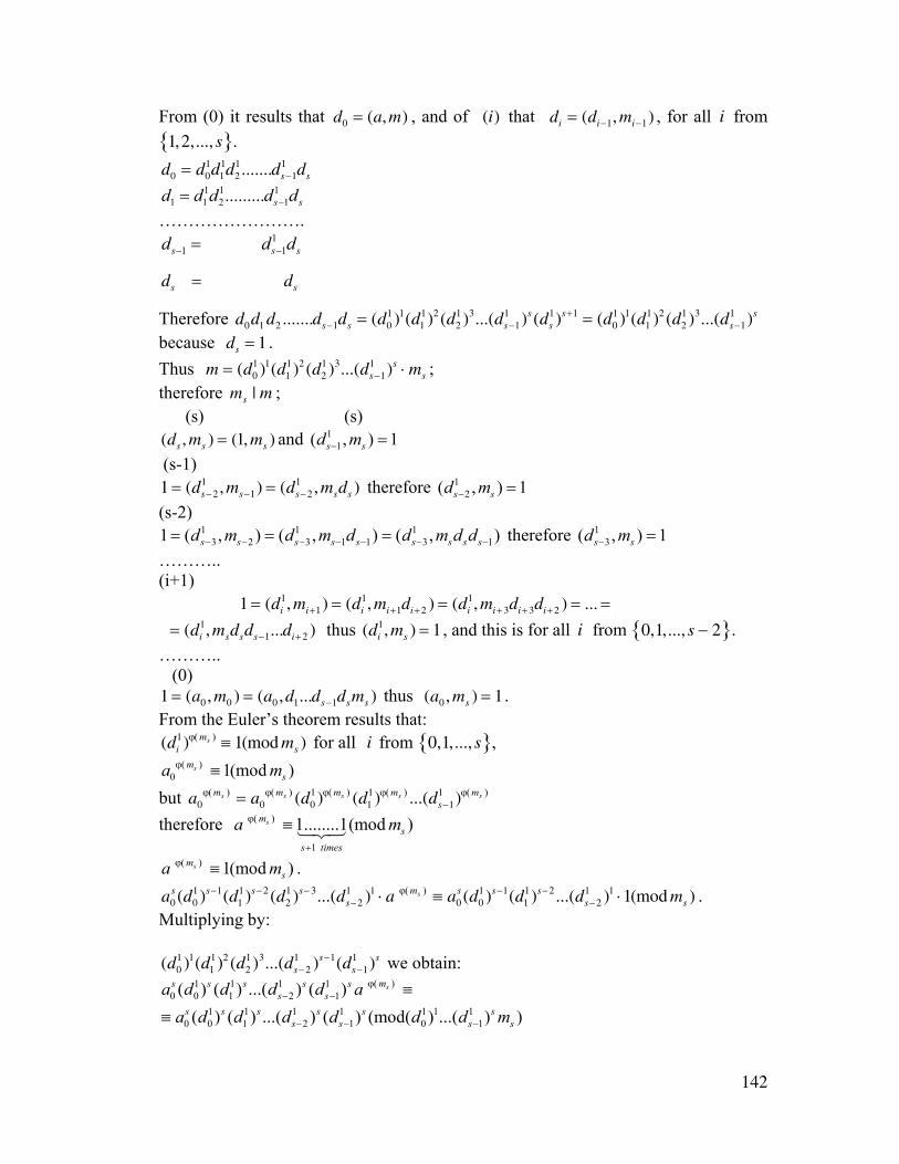
142
From (0) it results that d0 = (a,m) , and of (i) that di = (di−1, mi−1) , for all i from 1,2,..., s{ }.
d0 = d01d1
1d21.......ds−1
1 ds 1 1 1
1 1 2 1......... s sd d d d d−= …………………….
11 1s s sd d d− −=
ds = ds
Therefore d0d1 d2 .......ds−1ds = (d01 )1(d1
1)2 (d21 )3...(ds−1
1 )s (ds1)s+1 = (d0
1 )1(d11)2 (d2
1 )3...(ds−11 )s
because ds = 1 . Thus m = (d0
1 )1(d11)2 (d2
1 )3...(ds−11 )s ⋅ ms ;
therefore ms | m ; (s) (s) (ds , ms ) = (1, ms ) and 1
1( , ) 1s sd m− = (s-1) 1 = (ds−2
1 , ms−1) = (ds−21 , msds ) therefore 1
2( , ) 1s sd m− = (s-2)
1 1 13 2 3 1 1 3 11 ( , ) ( , ) ( , )s s s s s s s s sd m d m d d m d d− − − − − − −= = = therefore 1
3( , ) 1s sd m− = ……….. (i+1) 1 = (di
1, mi+1) = (di1, mi+1di+2 ) = (di
1, mi+ 3di+ 3di+2 ) = ... = = (di
1, msdsds−1...di+2 ) thus (di1, ms ) = 1 , and this is for all i from 0,1,..., s − 2{ }.
……….. (0) 1 = (a0 , m0 ) = (a0 ,d1...ds−1dsms ) thus (a0 , ms ) = 1 . From the Euler’s theorem results that: (di
1)ϕ(ms ) ≡ 1(mod ms ) for all i from 0,1,..., s{ },
0 1(mod )smsa mϕ( ) ≡
but a0ϕ(ms ) = a0
ϕ(ms ) (d01 )ϕ(ms ) (d1
1)ϕ(ms ) ...(ds−11 )ϕ(ms )
therefore 1
1........1(mod )sms
s times
a mϕ( )
+
≡
1(mod )smsa mϕ( ) ≡ .
a0s (d0
1 )s−1(d11)s−2 (d2
1 )s− 3...(ds−21 )1 ⋅ a ϕ(ms ) ≡ a0
s (d01 )s−1(d1
1)s−2 ...(ds−21 )1 ⋅1(mod ms ) .
Multiplying by: (d0
1 )1(d11)2 (d2
1 )3...(ds−21 )s−1(ds−1
1 )s we obtain: 1 1 1 1
0 0 1 2 1( ) ( ) ...( ) ( ) sms s s s ss sa d d d d a ϕ( ) − − ≡
1 1 1 1 1 1 10 0 1 2 1 0 1( ) ( ) ...( ) ( ) (mod( ) ...( ) )s s s s s s
s s s sa d d d d d d m− − −≡
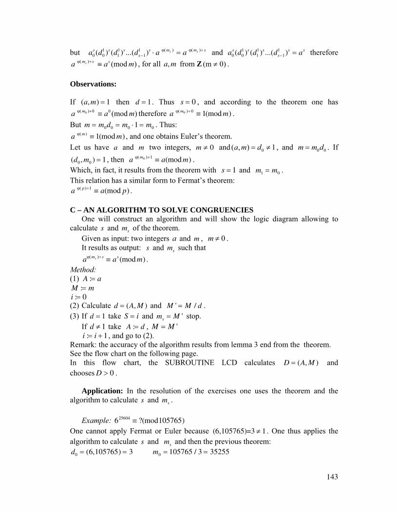
143
but a0s (d0
1 )s (d11)s ...(ds−1
1 )s ⋅ a ϕ(ms ) = a ϕ(ms )+ s and a0s (d0
1 )s (d11)s ...(ds−1
1 )s = as therefore (mod )sm s sa a mϕ( )+ ≡ , for all a,m from Z (m 0)≠ .
Observations: If (a,m) = 1 then d = 1 . Thus s = 0 , and according to the theorem one has
0 0 0 (mod )ma a mϕ( )+ ≡ therefore a ϕ(m0 )+0 ≡ 1(mod m) . But m = m0d0 = m0 ⋅1 = m0 . Thus: a ϕ(m ) ≡ 1(mod m) , and one obtains Euler’s theorem. Let us have a and m two integers, m ≠ 0 and 0( , ) 1a m d= ≠ , and 0 0m m d= . If (d0 , m0 ) = 1 , then a ϕ(m0 )+1 ≡ a(mod m) . Which, in fact, it results from the theorem with s = 1 and m1 = m0 . This relation has a similar form to Fermat’s theorem: a ϕ( p)+1 ≡ a(mod p) . C – AN ALGORITHM TO SOLVE CONGRUENCIES One will construct an algorithm and will show the logic diagram allowing to calculate s and ms of the theorem. Given as input: two integers a and m , 0m ≠ . It results as output: s and ms such that aϕ(ms ) + s ≡ as (mod m) . Method: (1) A := a M := m i := 0 (2) Calculate d = (A, M ) and M ' = M / d . (3) If d = 1 take S = i and ms = M ' stop. If d ≠ 1 take A := d , M = M ' i := i + 1 , and go to (2). Remark: the accuracy of the algorithm results from lemma 3 end from the theorem. See the flow chart on the following page. In this flow chart, the SUBROUTINE LCD calculates D = (A, M ) and chooses D > 0 . Application: In the resolution of the exercises one uses the theorem and the algorithm to calculate s and ms . Example: 625604 ≡ ?(mod105765) One cannot apply Fermat or Euler because (6,105765)=3 ≠ 1 . One thus applies the algorithm to calculate s and ms and then the previous theorem: d0 = (6,105765) = 3 m0 = 105765 / 3 = 35255
144
i = 0;3 ≠ 1 thus i = 0 + 1 = 1, d1 = (3,35255) = 1 , m1 = 35255 /1 = 35255 . Therefore 6ϕ(35255)+1 ≡ 61(mod105765) thus 625604 ≡ 64 (mod105765) .
* * *
*
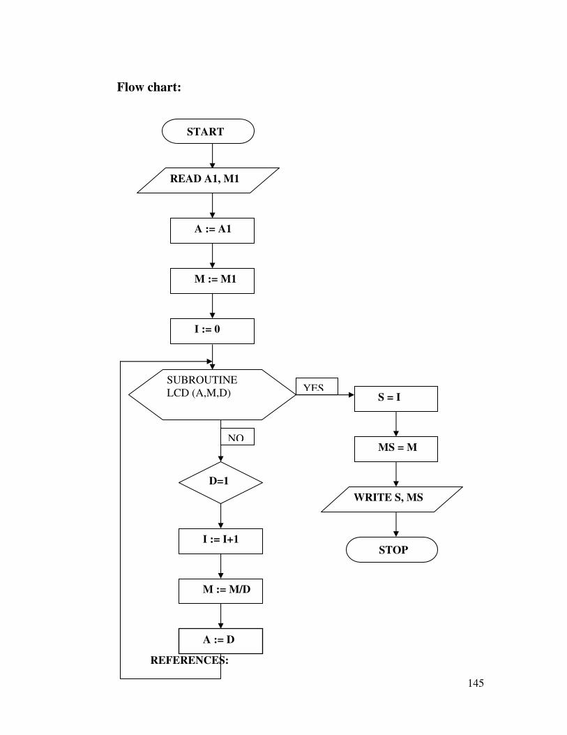
145
Flow chart:
REFERENCES:
START
READ A1, M1
A := A1
M := M1
I := 0
SUBROUTINE LCD (A,M,D)
NO
D=1
I := I+1
M := M/D
A := D
YES S = I
MS = M
WRITE S, MS
STOP
146
[1] Popovici, Constantin P. – “Teoria numerelor”, Curs, Bucharest, Editura
didactic i pedagogic , 1973. [2] Popovici, Constantin P – “Logica i teaoria numerelor”, Editura didactic
i pedagogic , Bucharest, 1970. [3] Creang I, Cazacu C, Mihu P, Opai Gh, Reischer Corina – “Introducere
în teoria numerelor”, Editura didactic i pedagogic , Bucharest, 1965. [4] Rusu E, - “Aritmetica i teoria numerelor”, Editura didactic i pedagogic ,
Editia a 2-a, Bucharest, 1963. [Published in “Bulet. Univ. Bra ov”, seria C, Vol. XXIII, 1981, pp. 7-12; MR: 84j:10006.]
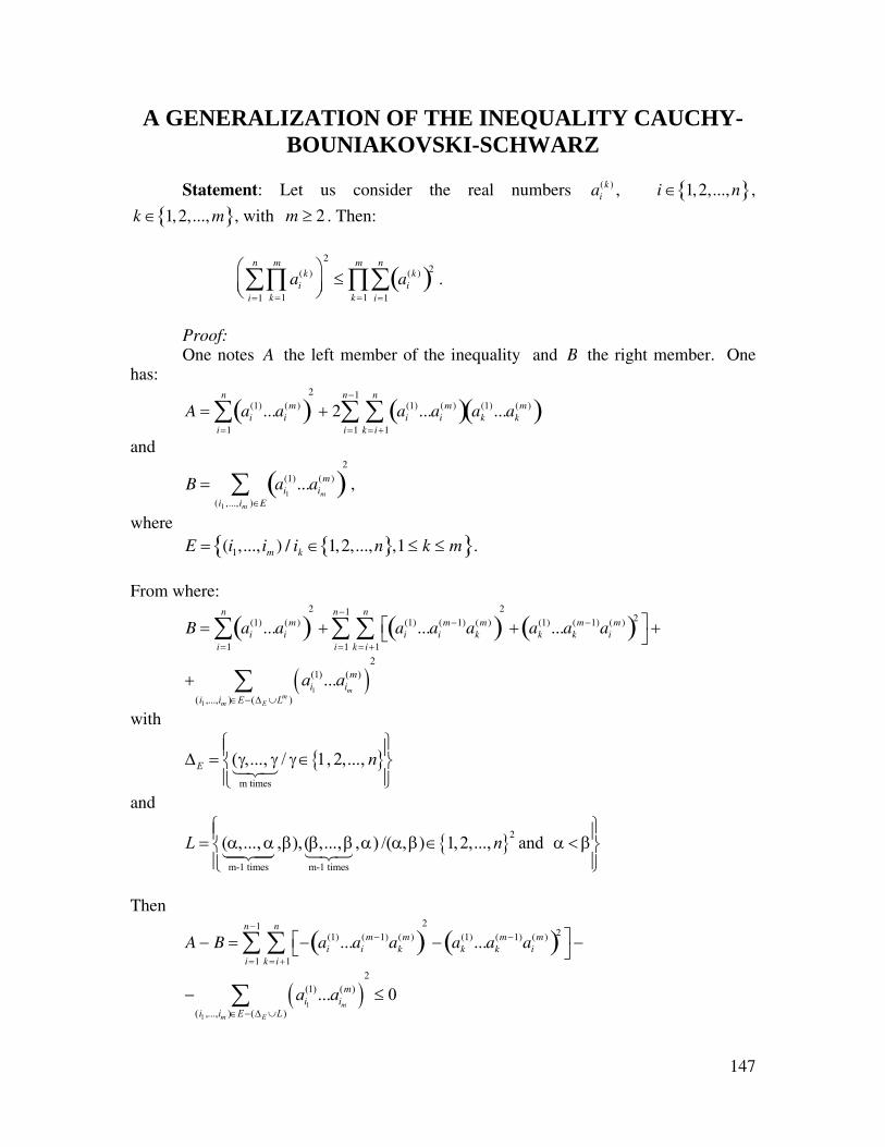
147
A GENERALIZATION OF THE INEQUALITY CAUCHY-BOUNIAKOVSKI-SCHWARZ
Statement: Let us consider the real numbers ai
(k ) , i ∈ 1,2,...,n{ },
k ∈ 1,2,..., m{ }, with m ≥ 2 . Then:
ai(k )
k =1
m
∏i=1
n
∑⎛⎝⎜
⎞⎠⎟
2
≤ ai(k )( )2
i=1
n
∑k =1
m
∏ .
Proof: One notes A the left member of the inequality and B the right member. One
has:
A = ai(1)...ai
(m )( )i=1
n
∑2
+ 2 ai(1)...ai
(m )( )k = i+1
n
∑i=1
n−1
∑ ak(1)...ak
(m )( )
and
B = ai1
(1)...aim
(m )( )(i1 ,...,im )∈E
∑2
,
where E = (i1,...,im ) / ik ∈ 1,2,...,n{ },1 ≤ k ≤ m{ }.
From where:
B = ai(1)...ai
(m )( )i=1
n
∑2
+ ai(1)...ai
(m−1)ak(m )( )⎡⎣
k = i+1
n
∑i=1
n−1
∑2
+ ak(1)...ak
(m−1)ai(m )( )2 ⎤
⎦ +
( )1
1
2(1) ( )
( ,..., ) ( )
...m
mm E
mi i
i i E L
a a∈ − Δ ∪
+ ∑
with
{ }m times
( /E n⎧ ⎫⎪ ⎪Δ = γ,..., γ γ ∈ 1,2,...,⎨ ⎬⎪ ⎪⎩ ⎭
and
{ }2
m-1 times m-1 times
( , ), ( , ) /( 1,2,..., andL n⎧ ⎫⎪ ⎪= α,...,α β β,...,β α α,β)∈ α < β⎨ ⎬⎪ ⎪⎩ ⎭
Then
A − B = − ai(1)...ai
(m−1)ak(m )( )⎡⎣
k = i+1
n
∑i=1
n−1
∑2
− ak(1)...ak
(m−1)ai(m )( )2 ⎤
⎦ −
( )1
1
2(1) ( )
( ,..., ) ( )... 0
m
m E
mi i
i i E La a
∈ − Δ ∪
− ≤∑
148
Note: for m = 2 one obtains the inequality of Cauchy-Bouniakovski-Schwarz.
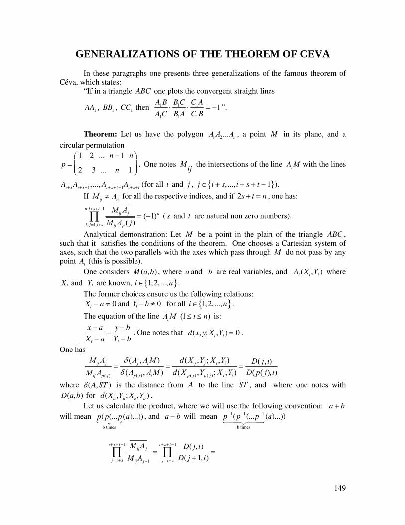
149
GENERALIZATIONS OF THE THEOREM OF CEVA
In these paragraphs one presents three generalizations of the famous theorem of Céva, which states: “If in a triangle ABC one plots the convergent straight lines
AA1 , BB1 , CC1 then A1B
A1C⋅
B1C
B1A⋅C1A
C1B= −1“.
Theorem: Let us have the polygon 1 2... nA A A , a point M in its plane, and a circular permutation
p =1 2 ... n − 1 n
2 3 ... n 1
⎛
⎝⎜⎜
⎞
⎠⎟⎟. One notes M
ij the intersections of the line Ai M with the lines
Ai + s Ai + s+1,..., Ai + s+ t −1Ai+ s+ t (for all i and j , j ∈ i + s,..., i + s + t − 1{ }).
If ij nM A≠ for all the respective indices, and if 2s t n+ = , one has:
, 1
, 1,
( 1)( )
n i s tij j n
i j i s ij p
M AM A j
+ + −
= +
= −∏ ( s and t are natural non zero numbers).
Analytical demonstration: Let M be a point in the plain of the triangle ABC , such that it satisfies the conditions of the theorem. One chooses a Cartesian system of axes, such that the two parallels with the axes which pass through M do not pass by any point Ai (this is possible). One considers M (a,b) , where a and b are real variables, and Ai (Xi ,Yi ) where
Xi and Yi are known, i ∈ 1,2,...,n{ }. The former choices ensure us the following relations: Xi − a ≠ 0 and 0iY b− ≠ for all i ∈ 1,2,...,n{ }.
The equation of the line (1 )iA M i n≤ ≤ is:
x − a
Xi − a−
y − b
Yi − b. One notes that d(x, y; Xi ,Yi ) = 0 .
One has
( ) ( ) ( )( )
( , ) ( , ; , ) ( , )( , ) ( , ; , ) ( ( ), )
ij j j i j j i i
p j i p j p j i iij p j
M A A A M d X Y X Y D j iA A M d X Y X Y D p j iM A
δδ
= = =
where δ (A,ST ) is the distance from A to the line ST , and where one notes with D(a,b) for d(Xa ,Ya; Xb ,Yb ) . Let us calculate the product, where we will use the following convention: a + b will mean
p( p(...p
b times
(a)...)) , and a − b will mean p−1(p−1(...p−1
b times
(a)...))
Mij Aj
Mij Aj +1j = i+ s
i+ s+ t −1
∏ =D( j,i)
D( j + 1, i)j = i+ s
i+ s+ t −1
∏ =
150
( , ) ( 1, ) ( 1, )
( 1, ) ( 2, ) ( , )D i s i D i s i D i s t i
D i s i D i s i D i s t i+ + + + + −
= ⋅ ⋅⋅⋅ =+ + + + + +
=D(i + s,i)
D(i + s + t, i)=
D(i + s,i)
D(i − s,i)
The initial product is equal to:
D(i + s,i)
D(i − s,i)=
i=1
n
∏ D(1 + s,1)
D(1 − s,1)⋅
D(2 + s,2)
D(2 − s,2)⋅ ⋅ ⋅
D(2s, s)
D(n, s)⋅
⋅D(2s + 2, s + 2)
D(2, s + 2)⋅ ⋅ ⋅
D(2s + t, s + t)
D(t, s + t)⋅
D(2s + t + 1, s + t + 1)
D(t + 1, s + t + 1)⋅
⋅D(2s + t + 2, s + t + 2)
D(t + 2, s + t + 2)⋅ ⋅ ⋅
D(2s + t + s, s + t + s)
D(t + s, s + t + s)=
=D(1+ s,1)
D(1,1+ s)⋅
D(2 + s,2)
D(2,2 + s)⋅ ⋅ ⋅
D(2s + t, s + t)
D(s + t,2s + t)⋅ ⋅ ⋅
D(s,n)
D(n, s)=
=D(i + s, i)
D(i,i + s)=
i=1
n
∏ −P(i + s)
P(i)
⎛⎝⎜
⎞⎠⎟i=1
n
∏ = (−1)n
because:
( )( )( , ) ( )
( , ) ( )( ) ( )
r r
p p r r
p p p p
r r
X a Y bX a Y b X a Y bD r p P rX a Y bD p r X a Y b P pX a Y b
− −−
− − − −= = − = −
− − − −−− −
,
The last equality resulting from what one notes: (Xt − a)(Yt − b) = P(t) . From (1)
it results that P(t) ≠ 0 for all t from { }1,2,...,n . The proof is completed.
Comments regarding the theorem: t represents the number of lines of a polygon which are intersected by a line
Ai0M ; if one notes the sides AiAi+1 of the polygon, by ai , then s + 1 represents the
order of the first line intersected by the line A1M (that is as+1 the first line intersected by A1M ).
Example: If s = 5 and t = 3 , the theorem says that :
- the line A1M intersects the sides 6 7 7 8 8 9, ,A A A A A A .
- the line A2M intersects the sides 7 8 8 9 9 10, ,A A A A A A .
- the line A3M intersects the sides 8 9 9 10 10 11, ,A A A A A A , etc.
151
Observation: The restrictive condition of the theorem is necessary for the
existence of the ratios ( )
ij j
ij p j
M AM A
.
Consequence 1: Let us have a polygon A1A2 ...A2k +1 and a point M in its plan.
For all i from 1,2,...,2k + 1{ }, one notes Mi the intersection of the line Ai Ap(i ) with
the line which passes through M and by the vertex which is opposed to this line. If
Mi ∉ Ai , Ap(i ){ } then one has: Mi Ai
Mi Ap(i )i=1
n
∏ = −1.
The demonstration results immediately from the theorem, since one has s = k and t = 1, that is n = 2k + 1 . The reciprocal of this consequence is not true.
From where it results immediately that the reciprocal of the theorem is not true either. Counterexample:
Let us consider a polygon of 5 sides. One plottes the lines A1M 3, A2M 4 and A3M 5 which intersect in M .
Let us have K =M 3A3
M 3A4
⋅M 4 A4
M 4 A5
⋅M 5A5
M 5A1
Then one plots the line A4 M1 such that it does not pass through M and such that it forms the ratio:
(2) M1A1
M1A2
= 1 / K or 2 / K . (One chooses one of these values, for which
A4 M1 does not pass through M ).
At the end one traces A5M 2 which forms the ratio M 2A2
M 2A3
= −1 or −1
2 in
function of (2). Therefore the product: Mi Ai
Mi Ap(i )i=1
5
∏ without which the respective lines are concurrent.
Consequence 2: Under the conditions of the theorem, if for all i and j, j ∉ i, p−1(i){ }, one notes Mij = Ai M ∩ Aj Ap( j ) and Mij ∉ Aj , Ap( j ){ } then one has:
Mij Aj
Mij Ap( j )i, j =1
n
∏ = (−1)n .
j ∉ i, p−1(i){ }
In effect one has s = 1 , t = n − 2 , and therefore 2s + t = n .
152
Consequence 3: For n = 3, it comes s = 1 and t = 1, therefore one obtains (as a particular case ) the theorem of Céva.
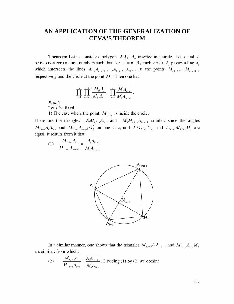
153
AN APPLICATION OF THE GENERALIZATION OF CEVA’S THEOREM
Theorem: Let us consider a polygon A1A2 ...An inserted in a circle. Let s and t be two non zero natural numbers such that 2s + t = n . By each vertex Ai passes a line di which intersects the lines Ai+ sAi+ s+1,...., Ai+ s+ t −1Ai+ s+ t at the points Mi,i+ s ,..., Mi+ s+t −1
respectively and the circle at the point Mi' . Then one has:
'1
'1 11
n i s t nij j i i s
i j i s iij j i i s t
M A M AM A M A
+ + −+
= = + =+ + +
=∏ ∏ ∏ .
Proof: Let i be fixed.
1) The case where the point Mi,i+ s is inside the circle.
There are the triangles AiMi,i+ sAi+ s and Mi'Mi,i+ sAi+ s+1 similar, since the angles
Mi,i+ sAiAi+ s and Mi,i + s Ai+ s+1Mi' on one side, and AiMi,i+ sAi+ s and Ai + s+1Mi,i + s Mi
' are equal. It results from it that:
(1) Mi ,i+ sAi
Mi,i+ sAi+ s+1
=Ai Ai+ s
Mi'Ai+ s+1
Ai+s+1 Ai MMM Mi
' Ai+s
In a similar manner, one shows that the triangles Mi,i+ sAiAi+ s+1 and Mi,i + s Ai + s Mi'
are similar, from which:
(2) Mi,i+ sAi
Mi,i+ sAi+ s
=Ai Ai+ s+1
Mi'Ai+ s
. Dividing (1) by (2) we obtain:
Mi,i+s
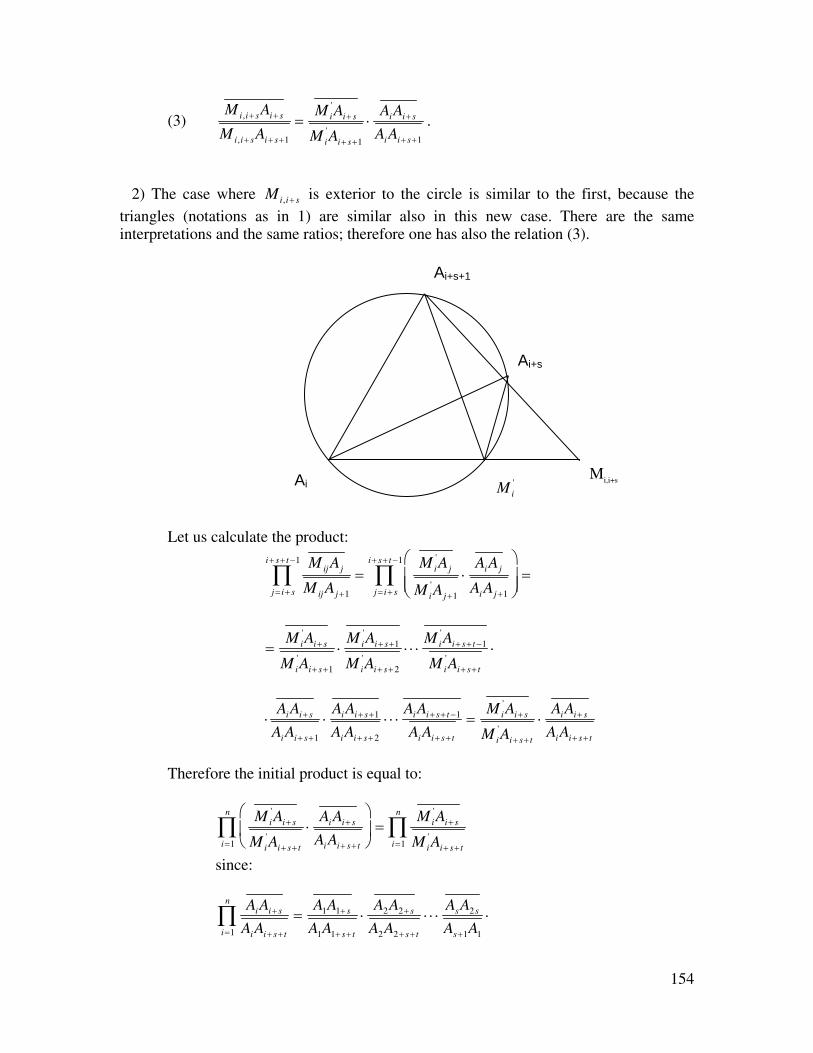
154
(3) Mi,i+ sAi+ s
Mi,i+ sAi+ s+1
=Mi
'Ai+ s
Mi'Ai+ s+1
⋅Ai Ai+ s
Ai Ai+ s+1
.
2) The case where Mi,i+ s is exterior to the circle is similar to the first, because the triangles (notations as in 1) are similar also in this new case. There are the same interpretations and the same ratios; therefore one has also the relation (3).
Let us calculate the product:
Mij Aj
Mij Aj +1j = i+ s
i+ s+ t −1
∏ =Mi
'Aj
Mi'Aj +1
⋅Ai Aj
Ai Aj +1
⎛
⎝⎜⎜
⎞
⎠⎟⎟j = i+ s
i+ s+ t −1
∏ =
=Mi
'Ai+ s
Mi'Ai+ s+1
⋅Mi
'Ai+ s+1
Mi'Ai+ s+2
⋅ ⋅ ⋅Mi
'Ai+ s+ t −1
Mi'Ai+ s+ t
⋅
⋅Ai Ai+ s
Ai Ai+ s+1
⋅Ai Ai+ s+1
Ai Ai+ s+2
⋅ ⋅ ⋅Ai Ai+ s+ t −1
Ai Ai+ s+ t
=Mi
'Ai+ s
Mi'Ai+ s+ t
⋅Ai Ai+ s
Ai Ai+ s+ t
Therefore the initial product is equal to:
Mi
'Ai+ s
Mi'Ai+ s+ t
⋅Ai Ai+ s
Ai Ai+ s+ t
⎛
⎝⎜
⎞
⎠⎟
i=1
n
∏ =Mi
'Ai+ s
Mi'Ai+ s+ ti=1
n
∏
since:
Ai Ai+ s
Ai Ai+ s+ ti=1
n
∏ =A1A1+ s
A1A1+ s+ t
⋅A2A2+ s
A2A2+ s+ t
⋅ ⋅ ⋅AsA2 s
As+1A1
⋅
Ai+s+1
Ai+s
Mi'
Mi,i+s Ai
155
⋅As+2A2s+2
As+2A2
⋅ ⋅ ⋅As+ t An
As+ t At
⋅As+ t +1A1
As+ t +1At +1
⋅As+ t + 2A2
As+ t +2At +2
⋅ ⋅ ⋅AnAs
AnAs+ t
= 1
(by taking into account the fact that 2s + t = n ). Consequence 1: If there is a polygon A1A2 ,...., A2 s−1 inscribed in a circle, and from each vertex Ai one traces a line di which intersects the opposite side Ai + s−1Ai+ s in
M i and the circle in Mi' then:
Mi Ai+ s−1
Mi Ai+ si=1
n
∏ =Mi
'Ai+ s−1
Mi'Ai+ si=1
n
∏
In fact for t = 1, one has n odd and s =n + 1
2.
If one makes s = 1 in this consequence, one finds the mathematical note from [1], pages 35-37. Application: If in the theorem, the lines di are concurrent, one obtains:
Mi
'Ai+ s
Mi'Ai+ s+ ti=1
n
∏ = (−1)n (For this, see [2]).
Bibliography: [1] Dan Barbilian (Ion Barbu) – “Pagini inedite”, Editura Albatros, Bucharest, 1981 (Ediţie îngrijită de Gerda Barbilian, V. Protopopescu, Viorel Gh. Vodă). [2] Florentin Smarandache – “Généralisation du théorème de Céva”.
156
A GENERALIZATION OF A THEOREM OF CARNOT
Theorem of Carnot: Let M be a point on the diagonal AC of an arbitrary quadrilateral ABCD . Through M one draws a line which intersects AB in α and BC in β . Let us draw another line, which intersects CD in γ and AD in δ . Then one has:
AαBα
⋅BβCβ
⋅CγDγ
⋅DδAδ
= 1.
Generalization: Let 1... nA A be a polygon. On a diagonal A1Ak of this polygon one takes a point M through which one draws a line d1 which intersects the lines A1A2 , A2 A3,..., Ak −1Ak respectively in the points P1, P2 ,..., Pk −1 and another line d2 intersects the other lines Ak Ak +1,,..., An−1An , AnA1 respectively in the points Pk ,..., Pn−1, Pn . Then one has:
1 ( )
1n
i i
i i i
A PA Pϕ=
=∏ ,
where ϕ is the circular permutation
1 2 ... n − 1 n
2 3 ... n 1
⎛
⎝⎜⎜
⎞
⎠⎟⎟
.
Proof: Let us have 1 ≤ j ≤ k − 1. One easily shows that:
AjPj
Aj +1Pj
=D(Aj ,d1)
D(Aj +1,d1)
where D(A,d) represents the distance from the point A to the line d , since the
triangles Pj Aj Aj' and Pj Aj +1Aj +1
' are similar. (One notes with Aj' and Aj +1
' the projections
of the points Aj and Aj +1 on the line d1 ).
It results from it that:
A1P1
A2P1
⋅A2P2
A3P2
⋅ ⋅ ⋅Ak −1Pk −1
AkPk −1
=D(A1,d1)
D(A2 ,d1)⋅
D(A2 ,d1)
D(A3,d1)⋅ ⋅ ⋅
D(Ak −1,d1)
D(Ak ,d1)=
D(A1,d1)
D(Ak ,d1)
In a similar way, for k ≤ h ≤ n one has:
AhPh
Aϕ (h)Ph
=D(Ah ,d2 )
D(Aϕ (h),d2 )
and
AhPh
Aϕ (h)Phh= k
n
∏ =D(Ak ,d2 )
D(A1,d2 )
157
The product of the theorem is equal to:
D(A1,d1)
D(Ak ,d1)⋅
D(Ak ,d2 )
D(A1,d2 ),
but
D(A1,d1)
D(Ak ,d1)=
A1M
Ak M
since the triangles MA1A1' and MAk Ak
' are similar. In the same way, because the
triangles MA1A1'' and MAk Ak
'' are similar (one notes with A1'' and Ak
'' the respective projections of A1 and Ak on the line d2 ), one has:
D(Ak ,d2 )
D(A1,d2 )=
Ak M
A1M.
The product from the statement is therefore equal to 1. Remark: If one replaces n by 4 in this theorem, one finds the theorem of Carnot.
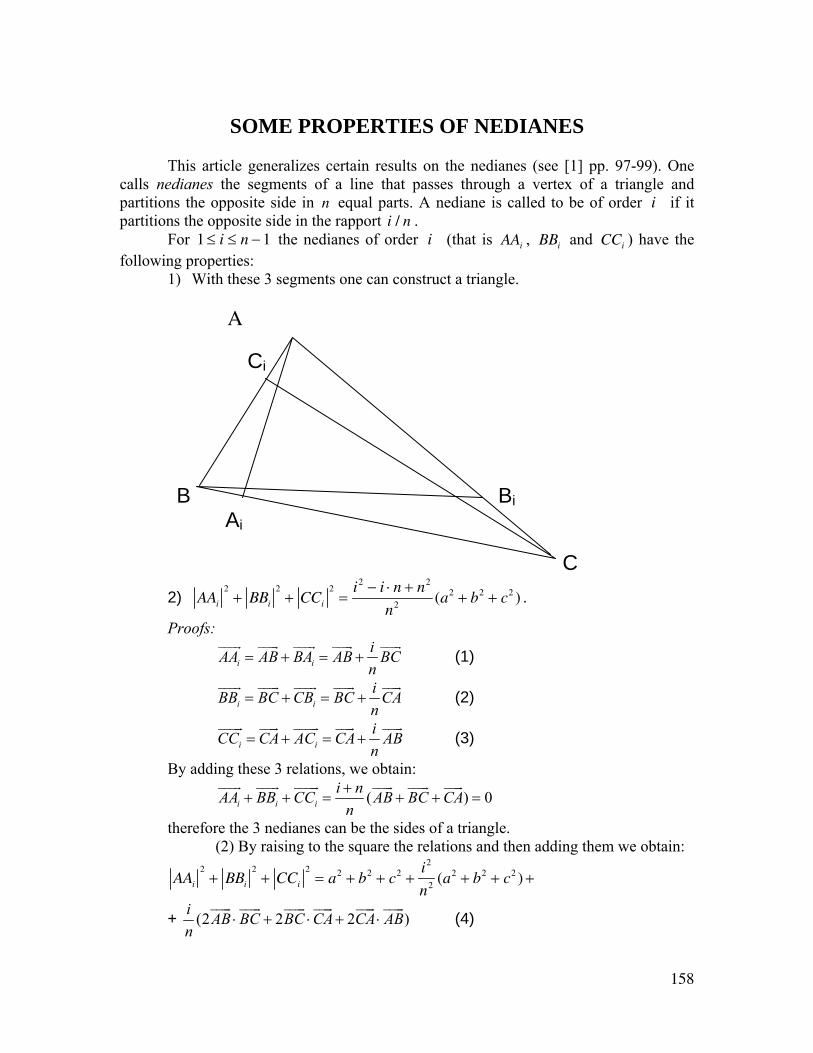
158
SOME PROPERTIES OF NEDIANES This article generalizes certain results on the nedianes (see [1] pp. 97-99). One calls nedianes the segments of a line that passes through a vertex of a triangle and partitions the opposite side in n equal parts. A nediane is called to be of order i if it partitions the opposite side in the rapport i / n . For 1 ≤ i ≤ n − 1 the nedianes of order i (that is AAi , BBi and CCi ) have the following properties:
1) With these 3 segments one can construct a triangle.
A Ci B Bi Ai C 2) AAi
2+ BBi
2+ CCi
2=
i2 − i ⋅ n + n2
n2 (a2 + b2 + c2 ) .
Proofs:
i iiAA AB BA AB BCn
= + = + (1)
i iiBB BC CB BC CAn
= + = + (2)
i iiCC CA AC CA ABn
= + = + (3)
By adding these 3 relations, we obtain:
( ) 0i i ii nAA BB CC AB BC CA
n+
+ + = + + =
therefore the 3 nedianes can be the sides of a triangle. (2) By raising to the square the relations and then adding them we obtain:
AAi
2+ BBi
2+ CCi
2= a2 + b2 + c2 +
i2
n2 (a2 + b2 + c2 ) +
+ (2 2 2 )i AB BC BC CA CA ABn
⋅ + ⋅ + ⋅ (4)
159
Because 2 2 22 2 cosAB BC ca B b c a⋅ = − ⋅ = − − (the theorem of cosines), by
substituting this in the relation (4), we obtain the requested relation. REFERENCE: [1] Vodă, Dr. Viorel Gh. – “Surprize în matematica elementară”, Editura Albatros,
Bucharest, 1981.
160
GENERALIZATIONS OF DEGARGUES THEOREM*
Let’s consider the points A1,..., An situated on the same plane, and B1,..., Bn situated on another plane, such that the lines Ai Bi are concurrent. Let’s prove that if the lines Ai Aj and BiBj are concurrent, then their intersecting points are collinear. Solution. Let α be the plane that contains the points A1,..., An (in the case in which the points are non-collinear α is unique), and analogously, let β = P(B1,..., Bn ) , and consider α ∩ β = d . Because the lines AiAj and BiBj are concurrent, Ai Aj ⊂ α , and Bi Bj ⊂ β , therefore their intersection belongs to line d . Remark 1. For n = 3 and A1, A2 , A3 non-collinear, B1, B2 , B3 non-collinear, and Ai ≠ Bj we obtain Desargues theorem. Remark 2. An extension of this generalization is: If we consider A1,..., An situated in a plane, and B1,..., Bm situated on another plane, prove that if Ai Aj and Bk Br are concurrent, then their intersection points are concurrent. Remark 3. For n = m , and Ai Bi concurrent lines, we obtain the first generalization. Remark 4. If in addition we also have n = m = 3 along with the previous conditions, we obtain the Desargues theorem. * Gamma, Anul X, nr. 1-2, Oct. 1987.
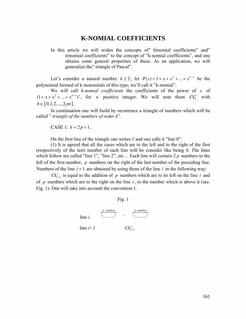
161
K-NOMIAL COEFFICIENTS
In this article we will widen the concepts of” binomial coefficients” and” trinomial coefficients” to the concept of ”k-nomial coefficients”, and one obtains some general properties of these. As an application, we will generalize the” triangle of Pascal”.
Let’s consider a natural number k ≥ 2 ; let P(x) = 1 + x + x2 + ... + xk −1 be the polynomial formed of k monomials of this type; we’ll call it ”k-nomial”. We will call k-nomial coefficients the coefficients of the power of x of (1 + x + x2 + ... + xk −1)n , for n positive integer. We will note them Ckn
h with h ∈ 0,1,2,...,2 pn{ }. In continuation one will build by recurrence a triangle of numbers which will be called ” triangle of the numbers of order k”. CASE 1: k = 2 p + 1. On the first line of the triangle one writes 1 and one calls it ”line 0”.
(1) It is agreed that all the cases which are to the left and to the right of the first (respectively of the last) number of each line will be consider like being 0. The lines which follow are called ”line 1”, ”line 2”, etc… Each line will contain 2 p numbers to the left of the first number, p numbers on the right of the last number of the preceding line. Numbers of the line i + 1 are obtained by using those of the line i in the following way: Cki+1
j is equal to the addition of p numbers which are to its left on the line i and of p numbers which are to the right on the line i , to the number which is above it (see. Fig. 1). One will take into account the convention 1.
Fig. 1
line i p numbers p numbers
⋅⋅ ⋅ ⋅ ⋅ ⋅ ⋅ ⋅ ⋅ ⋅ ⋅ ⋅ ⋅ ⋅ ⋅ ⋅ii i i i
line i+1 ⋅Cki+1j
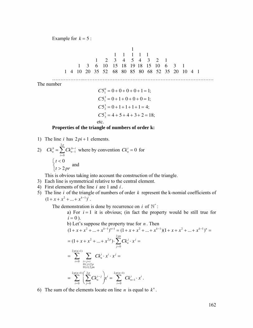
162
Example for k = 5 :
………………..……………………………………………………………………
The number C51
0 = 0 + 0 + 0 + 0 + 1 = 1;
C513 = 0 + 1+ 0 + 0 + 0 = 1;
C523 = 0 + 1+ 1+ 1+ 1 = 4;
C537 = 4 + 5 + 4 + 3 + 2 = 18;
etc. Properties of the triangle of numbers of order k:
1) The line i has 2 pi + 1 elements.
2) Cknh = Ckn−1
h− i
i=0
2 p
∑ where by convention Cknt = 0 for
t < 0
t > 2 pr
⎧⎨⎩
and
This is obvious taking into account the construction of the triangle. 3) Each line is symmetrical relative to the central element. 4) First elements of the line i are 1 and i . 5) The line i of the triangle of numbers of order k represent the k-nomial coefficients of
(1 + x + x2 + ...+ xk −1)i . The demonstration is done by recurrence on i of
* : a) For i = 1 it is obvious; (in fact the property would be still true for i = 0 ). b) Let’s suppose the property true for n . Then (1 + x + x2 + ... + xk −1)n+1 = (1 + x + x2 + ... + xk −1)(1 + x + x2 + ... + xk −1)n =
= (1+ x + x2 + ...+ x2 p ) ⋅ Cknj
j =0
2 pn
∑ ⋅ x j =
= Ckni
i+ j = t0≤ j ≤2 p0≤i≤2 pn
∑t = 0
2 p(n+1)
∑ ⋅ xi ⋅ x j =
= Cknt − j
j =0
2 p
∑⎛
⎝⎜⎞
⎠⎟t =0
2 p(n+1)
∑ xt = Ckn+1t
t =0
2 p(n+1)
∑ ⋅ xt .
6) The sum of the elements locate on line n is equal to kn .
1 1 1 1 1 1
1 2 3 4 5 4 3 2 1 1 3 6 10 15 18 19 18 15 10 6 3 1 1 4 10 20 35 52 68 80 85 80 68 52 35 20 10 4 1
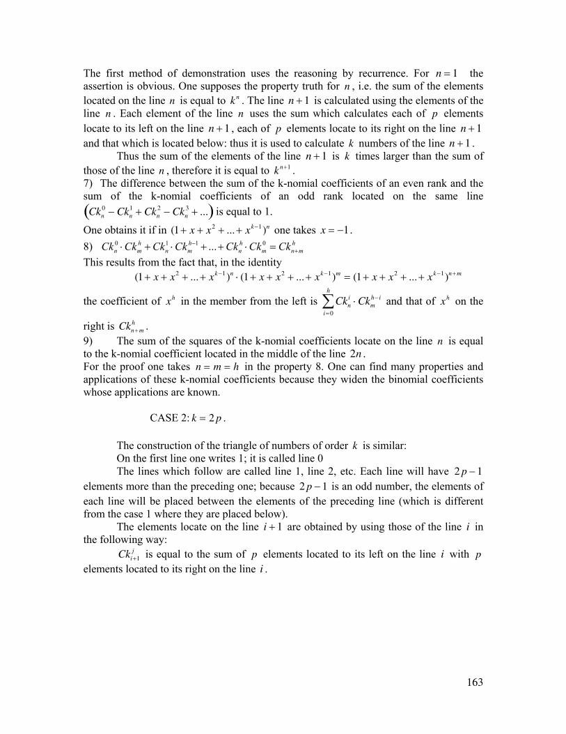
163
The first method of demonstration uses the reasoning by recurrence. For n = 1 the assertion is obvious. One supposes the property truth for n , i.e. the sum of the elements located on the line n is equal to kn . The line n + 1 is calculated using the elements of the line n . Each element of the line n uses the sum which calculates each of p elements locate to its left on the line n + 1 , each of p elements locate to its right on the line n + 1 and that which is located below: thus it is used to calculate k numbers of the line n + 1 .
Thus the sum of the elements of the line n + 1 is k times larger than the sum of those of the line n , therefore it is equal to kn+1 . 7) The difference between the sum of the k-nomial coefficients of an even rank and the sum of the k-nomial coefficients of an odd rank located on the same line Ckn
0 − Ckn1 + Ckn
2 − Ckn3 + ...( ) is equal to 1.
One obtains it if in (1 + x + x2 + ... + xk −1)n one takes x = −1. 8) 0 1 1 0...h h h h
n m n m n m n mCk Ck Ck Ck Ck Ck Ck−+⋅ + ⋅ + + ⋅ =
This results from the fact that, in the identity (1 + x + x2 + ... + xk −1)n ⋅ (1 + x + x2 + ... + xk −1)m = (1 + x + x2 + ... + xk −1)n+ m
the coefficient of xh in the member from the left is Ckni
i=0
h
∑ ⋅Ckmh− i and that of xh on the
right is Ckn+ mh .
9) The sum of the squares of the k-nomial coefficients locate on the line n is equal to the k-nomial coefficient located in the middle of the line 2n . For the proof one takes n = m = h in the property 8. One can find many properties and applications of these k-nomial coefficients because they widen the binomial coefficients whose applications are known.
CASE 2: k = 2 p . The construction of the triangle of numbers of order k is similar: On the first line one writes 1; it is called line 0 The lines which follow are called line 1, line 2, etc. Each line will have 2 p − 1 elements more than the preceding one; because 2 p − 1 is an odd number, the elements of each line will be placed between the elements of the preceding line (which is different from the case 1 where they are placed below). The elements locate on the line i + 1 are obtained by using those of the line i in the following way: Cki+1
j is equal to the sum of p elements located to its left on the line i with p elements located to its right on the line i .
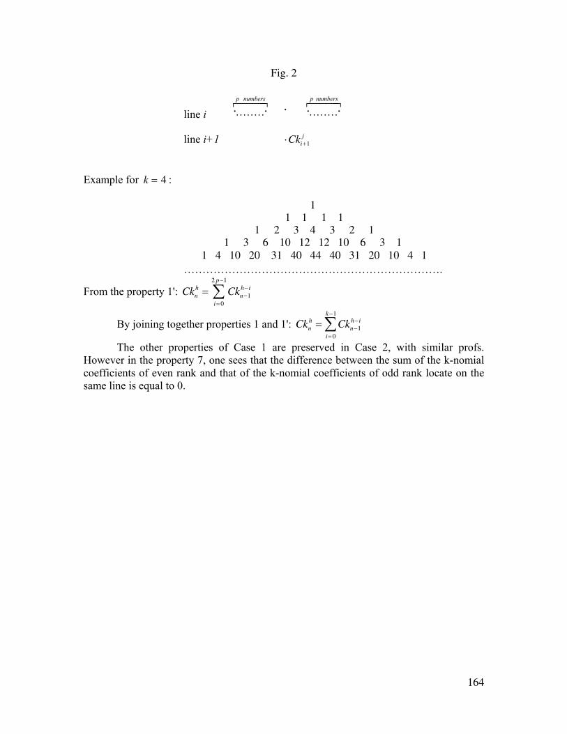
164
Fig. 2
line i p numbers p numbers
⋅⋅ ⋅ ⋅ ⋅ ⋅ ⋅ ⋅ ⋅ ⋅ ⋅ ⋅ ⋅ ⋅ ⋅ ⋅ii i i i
line i+1 ⋅Cki+1j
Example for k = 4 :
…………………………………………………………….
From the property 1': Cknh = Ckn−1
h− i
i=0
2 p−1
∑
By joining together properties 1 and 1': Cknh = Ckn−1
h− i
i=0
k −1
∑
The other properties of Case 1 are preserved in Case 2, with similar profs. However in the property 7, one sees that the difference between the sum of the k-nomial coefficients of even rank and that of the k-nomial coefficients of odd rank locate on the same line is equal to 0.
1 1 1 1 1 1 2 3 4 3 2 1 1 3 6 10 12 12 10 6 3 1 1 4 10 20 31 40 44 40 31 20 10 4 1
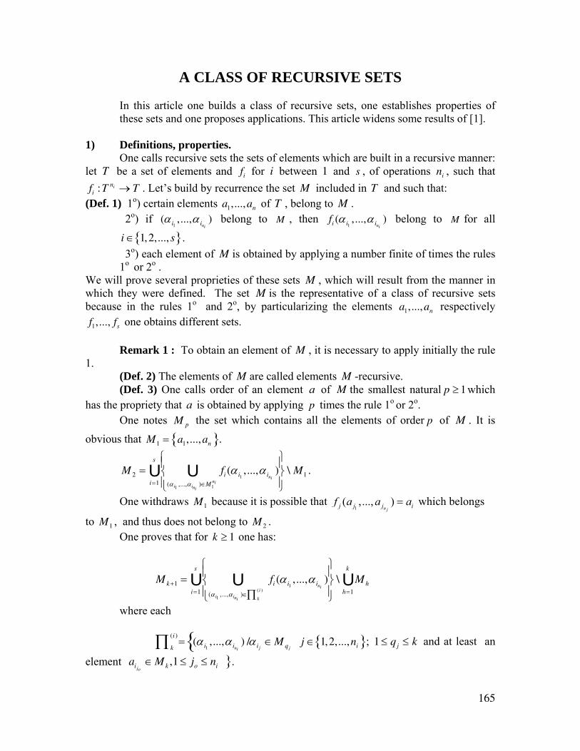
165
A CLASS OF RECURSIVE SETS
In this article one builds a class of recursive sets, one establishes properties of these sets and one proposes applications. This article widens some results of [1].
1) Definitions, properties.
One calls recursive sets the sets of elements which are built in a recursive manner: let T be a set of elements and fi for i between 1 and s , of operations ni , such that fi :T ni → T . Let’s build by recurrence the set M included in T and such that:
(Def. 1) 1o) certain elements a1,...,an of T , belong to M . 2o) if (α i1
,...,α ini) belong to M , then fi (α i1
,...,α ini) belong to M for all
i ∈ 1,2,..., s{ }. 3o) each element of M is obtained by applying a number finite of times the rules 1o or 2o .
We will prove several proprieties of these sets M , which will result from the manner in which they were defined. The set M is the representative of a class of recursive sets because in the rules 1o and 2o, by particularizing the elements a1,...,an respectively f1,..., fs one obtains different sets.
Remark 1 : To obtain an element of M , it is necessary to apply initially the rule
1. (Def. 2) The elements of M are called elements M -recursive. (Def. 3) One calls order of an element a of M the smallest natural p ≥ 1which
has the propriety that a is obtained by applying p times the rule 1o or 2o. One notes M p the set which contains all the elements of order p of M . It is
obvious that M1 = a1,...,an{ }.
M 2 = fi (α i1,...,α ini
)(α i1
,...,αini)∈M1
ni
U⎧⎨⎪
⎩⎪
⎫⎬⎪
⎭⎪i=1
s
U \ M1 .
One withdraws M1 because it is possible that 1
( ,..., )n jj j j if a a a= which belongs
to M1 , and thus does not belong to M 2 . One proves that for k ≥ 1 one has:
M k +1 = fi (α i1,...,α ini
)(αi1
,...,αini)∈
k
( i )∏U
⎧⎨⎪
⎩⎪
⎫⎬⎪
⎭⎪i=1
s
U \ Mhh=1
k
U
where each = (α i1
,...,α ini) /{k
(i )∏ α i j∈M qj
j ∈ 1,2,...,ni{ }; 1 ≤ qj ≤ k and at least an
element aijo∈M k ,1 ≤ jo ≤ ni }.
166
The sets M p , p ∈ * , form a partition of the set M .
Theorem 1:
M = M p
p∈ *U , where
* = 1,2, 3,...{ }.
Proof: From the rule 1o it results that M1 ⊆ M . One supposes that this propriety is true for values which are less than p . It results
that M p ⊆ M , because M p is obtained by applying the rule 2o to the elements of
Mii=1
p−1
U .
Thus
M pp∈ *U ⊆ M . Reciprocally, one has the inclusion in the contrary sense in
accordance with the rule 3o. Theorem 2: The set M is the smallest set, which has the properties 1o and 2o. Proof: Let R be the smallest set having properties 1o and 2o. One will prove that this set
is unique. Let’s suppose that there exists another set R ' having properties 1o and 2o, which is
the smallest. Because R is the smallest set having these proprieties, and because R ' has these properties also, it results that R ⊆ R ' ; of an analogue manner, we have R ' ⊆ R : therefore R = R ' .
It is evident that M ' ⊆ R . One supposes that M i ⊆ R for 1 ≤ i < p . Then (rule 3o), and taking in consideration the fact that each element of M p is obtained by applying rule 2o to certain elements of Mi , 1 ≤ i < p , it results that pM R⊆ . Therefore
*( )pp
M R p⊆ ∈∪ , thus M ⊆ R . And because R is unique, M = R .
Remark 2. The theorem 2 replaces the rule 3o of the recursive definition of the set M by: ” M is the smallest set that satisfies proprieties 1o and 2o”.
Theorem 3: M is the intersection of all the sets of T which satisfy conditions 1o
and 2o. Proof: Let T12 be the family of all sets of T satisfying the conditions 1o and 2o. We note
12A T
I A∈
= ∩ .
I has the properties 1o and 2o because: 1) For all i ∈ 1,2,...,n{ }, ai ∈ I , because ai ∈A for all A of T12 . 2) If α i1
,...,α ini∈ I , it results that α i1
,...,α inibelong to A that is A of T12 .
Therefore,
167
∀i ∈ 1,2,..., s{ }, fi (α i1,...,α ini
) ∈A which is A of T12 , therefore fi (α i1,...,α ini
) ∈ I
for all i from 1,2,..., s{ }. From theorem 2 it results that M ⊆ I . Because M satisfies the conditions 1o and 2o, it results that M ∈T12 , from which
I ⊆ M . Therefore M = I (Def. 4) A set A ⊆ I is called closed for the operation fi0
if and only if for all α i0 1,...,α i0 n i0
of A , one has fi0(α i0 1,...,α i0 n i0
) belong to A . (Def. 5) A set A ⊆ T is called M -recursively closed if and only if: 1) a1,...,an{ }⊆ A . 2) A is closed in respect to operations f1,..., fs . With these definitions, the precedent theorems become: Theorem 2’: The set M is the smallest M - recursively closed set. Theorem 3’: M is the intersection of all M - recursively closed sets. (Def. 6) The system of elements α1,...,αm , m ≥ 1 and α i ∈T for
i ∈ 1,2,...,m{ }, constitute a M -recursive description for the element α , if α m = α and that each α i ( i ∈ 1,2,...,m{ }) satisfies at least one of the proprieties:
1) α i ∈ a1,...,an{ }. 2) α i is obtained starting with the elements which precede it in the system by
applying the functions f j , 1 ≤ j ≤ s defined by property 2o of (Def. 1). (Def. 7) The number m of this system is called the length of the M -recursive
description for the element α . Remark 3: If the element α admits a M -recursive description, then it admits an
infinity of such descriptions. Indeed, if α1,...,αm is a M -recursive description of α then
1 1 1,..., , ,..., m
h times
a a α α is also a M -recursive description for α , h being able to take all
values from .
Theorem 4: The set M is identical with the set of all elements of T which admit a M -recursive description.
Proof: Let D be the set of all elements, which admit a M -recursive description. We will prove by recurrence that M p ⊆ D for all p of
* .
For p = 1 we have: M1 = a1,...,an{ }, and the aj , 1 ≤ j ≤ n , having as M -recursive description: < aj > . Thus M1 ⊆ D . Let’s suppose that the property is true for the values smaller than p . M p is obtained by applying the rule 2o to the elements of
168
1
1
;p
i pi
M Mα−
=
∈∪ implies that 1
( ,..., )nij i ifα α α∈ and α i j
∈M hj for hj < p and
1 ≤ j ≤ ni . But aij
, 1 ≤ j ≤ ni , admits M -recursive descriptions according to the hypothesis of
recurrence, let’s have 1,..., jj jsβ β . Then β11,...,β1s1,β21,...,β2 s2
,...,βni 1,...,βni sni,α
constitute a M -recursive description for the element α . Therefore if α belongs to D , then M p ⊆ D which is
M = M p
p∈ *U ⊆ D .
Reciprocally, let x belong to D . It admits a M -recursive description b1,...,bt with bt = x . It results by recurrence by the length of the M -recursive description of the element x , that x ∈M . For t = 1 we have b1 , b1 = x and b1 ∈ a1,...,an{ }⊆ M . One supposes that all elements y of D which admit a M -recursive description of a length inferior to t belong to M . Let x ∈D be described by a system of length t : b1,...,bt , bt = x . Then x ∈ a1,...,an{ }⊆ M , where x is obtained by applying the rule 2o to the elements which precede it in the system: b1,...,bt −1 . But these elements admit the M -recursive descriptions of length which is smaller that t : b1 , b1,b2 ,..., b1,...,bt −1 . According to the hypothesis of the recurrence, b1,...,bt −1 belong to M . Therefore bt belongs also to M . It results that M ≡ D . Theorem 5: Let b1,...,bq be elements of T, which are obtained from the elements a1,...,an by applying a finite number of times the operations
,,...,o sfff. Then M
can be defined recursively in the following mode: 1) Certain elements a1,...,an ,b1,...,bq of T belong to M . 2) M is closed for the applications fi , with i ∈ 1,2,..., s{ }. 3) Each element of M is obtained by applying a finite number of times the rules (1) or (2) which precede.
Proof: evident. Because b1,...,bq belong to T , and are obtained starting with the elements a1,...,an of M by applying a finite number of times the operations fi , it results that b1,...,bq belong to M .
Theorem 6: Let’s have gj , 1 ≤ j ≤ r , of the operations nj , where gj :T nj → T such that M to be closed in rapport to these operations. Then M can be recursively defined in the following manner: 1) Certain elements a1,...,an de T belong to M . 2) M is closed for the operations fi , i ∈ 1,2,..., s{ } and gj , j ∈ 1,2,...,r{ }. 3) Each element of M is obtained by applying a finite number of times the precedent rules. Proof is simple: Because M is closed for the operations gj (with j ∈ 1,2,...,r{ }), one has, that for any α j1,...,α j n j
from M , gj (α j1,...,α j n j) ∈M for all j ∈ 1,2,...,r{ }.
From the theorems 5 and 6 it results:
169
Theorem 7: The set M can be recursively defined in the following manner: 1) Certain elements a1,...,an ,b1,...,bq of T belong to M . 2) M is closed for the operations fi ( i ∈ 1,2,..., s{ }) and for the operations gj ( j ∈ 1,2,...,r{ }) previously defined. 3) Each element of M is defined by applying a finite number of times the previous 2 rules. (Def. 8) The operation fi conserves the property P iff for any elements α i1,...,α ini
having the property P , fi (α i1,...,α ini
) has the property P . Theorem 8 : If a1,...,an have the property P , and if the functions f1,..., fs
preserve this property, then all elements of M have the property P . Poof:
M = M p
p∈ *U . The elements of M1 have the property P .
Let’s suppose that the elements of Mi for i < p have the property P . Then the elements of M p also have this property because M p is obtained by applying the
operations f1, f2 ,..., fs to the elements of: Mii=1U , elements which have the property P .
Therefore, for any p of , the elements of M p have the property P . Thus all elements of M have it. Corollary 1 : Let’s have the property P : ” x can be represented in the form F(x) ”. If a1,...,an can be represented in the form F(a1),..., respectively F(an ) , and if
1,..., sf f maintains the property P , then all elements α of M can be represented in the form F(α ) .
Remark. One can find more other equivalent def. of M .
2) APPLICATIONS, EXAMPLES. In applications, certain general notions like: M - recursive element, M -recursive description, M - recursive closed set will be replaced by the attributes which characterize the set M . For example in the theory of recursive functions, one finds notions like: recursive primitive functions, primitive recursive description, primitively recursive closed sets. In this case ” M ” has been replaced by the attribute ”primitive” which characterizes this class of functions, but it can be replaced by the attributes ”general”, ”partial”. By particularizing the rules 1o and 2o of the def. 1, one obtains several interesting sets: Example 1: (see [2], pp. 120-122, problem 7.97). Example 2: The set of terms of a sequence defined by a recurring relation constitutes a recursive set.
170
Let’s consider the sequence: an+ k = f (an ,an+1,...,an+ k −1) for all n of * , with
0 , 1i ia a i k= ≤ ≤ . One will recursively construct the set A = am{ }m∈ * and one will
define in the same time the position of an element in the set A : 1°) a1
0 ,...,ak0 belong to A , and each ai
0 (1 ≤ i ≤ k ) occupies the position i in the set A ; 2°) if an ,an+1,...,an+ k −1 belong to A , and each aj for n ≤ j ≤ n + k − 1 occupies the position j in the set A , then f (an ,an+1,...,an+ k −1) belongs to A and occupies the position n + k in the set A . 3°) each element of B is obtained by applying a finite number of times the rules 1o or 2o. Example 3: Let G = e,a1,a2 ,...,a p{ } be a cyclic group generated by the element
a . Then ( ),G i can be recursively defined in the following manner:
1°) a belongs to G . 2°) if b and c belong to G then b ci belongs to G . 3°) each element of G is obtained by applying a finite number of times the rules 1 or 2. Example 4: Each finite set ML = x1, x2 ,..., xn{ } can be recursively defined (with ML ⊆ T ): 1°) The elements x1, x2 ,..., xn of T belong to ML . 2°) If a belongs to ML , then f (a) belongs to ML , where f :T → T such that f (x) = x ;
3°) Each element of ML is obtained by applying a finite number of times the rules 1° or 2°. Example 5: Let L be a vectorial space on the commutative corps K and
x1,..., xm{ } be a base of L . Then L , can be recursively defined in the following manner: 1°) x1,..., xm belong to L ; 2°) if x, y belong to L and if a belongs to K , then x ⊥ y y belong to L and a ∗ x belongs to L ;
3°) each element of L is recursively obtained by applying a finite number of times the rules 1° or 2°.
(The operators ⊥ and ∗ are respectively the internal and external operators of the vectorial space L ).
Example 6: Let X be an A -module, and M ⊂ X (M ≠ ∅) , with M = xi{ }i∈I.
The sub-module generated by M is:
{ }{ }1 1/ ... , , , 1,...,n n i iM x X x a x a x a A x M i n= ∈ = + + ∈ ∈ ∈
can be recursively defined in the following way: 1°) for all i of 1,2,...,n{ }, { }1,2,..., in x M∈i ; 2°) if x and y belong to M and a belongs to A , then x + y belongs to M , and ax also;
171
3°) each element of M is obtained by applying a finite number of times the rules 1° or 2°.
In accordance to the paragraph 1 of this article, M is the smallest sub-set of X that verifies the conditions 1° and 2°, that is M is the smallest sub-module of X that includes M . M is also the intersection of all the subsets of X that verify the conditions 1° and 2°, that is M is the intersection of all sub-modules of X that contain M . One also directly refines some classic results from algebra.
One can also talk about sub-groups or ideal generated by a set: one also obtains some important applications in algebra.
Example 7: One also obtains like an application the theory of formal languages, because, like it was mentioned, each regular language (linear at right) is a regular set and reciprocally. But a regular set on an alphabet Σ = a1,...,an{ } can be recursively defined in the following way:
1°) ∅, ε{ }, a1{ },..., an{ } belong to R . 2°) if P and Q belong to R , then P ∪ Q , PQ , and P∗ belong to R , with
{ }/ or P Q x x P x Q∪ = ∈ ∈ ; { }/ and PQ xy x P y Q= ∈ ∈ , and P∗ = Pn
n=0
∞
U with
n
n times
P P P P= ⋅ ⋅⋅⋅ and, by convention, P0 = ε{ }.
3°) Nothing else belongs to R other that those which are obtained by using 1° or 2°.
From which many properties of this class of languages with applications to the programming languages will result.
REFERENCES: [1] C. P. Popovici, L. Livovschi, H. Georgescu. N. Ţăndăreanu, ”Curs de
bazele informaticii (funcţii booleene şi circuite combinaţionale)”, Tipografia Universităţii din Bucureşti, 1976
[2] F. Smarandache, ”Problèmes avec et sans…problèmes!”, Somipress, Fès (Morocco), 1983.
172
A GENERALIZATION IN SPACE OF JUNG’S THEOREM
In this short note we will prove a generalization of Joung’s theorem in space. Theorem. Let us have n points in space such that the maximum distance
between any two points is a . Prove that there exists a sphere of radius r ≤ a6
4 that
contains in its interior or on its surface all these points. Proof: Let P1,..., Pn . be the points. Let S1(O1,r1) be a sphere of center O1 and radius r1 , which contains all these points. We note r2 = max
1≤i≤nPiO1 = P1O1 and construct the sphere
S2 (O1,r2 ) , r2 ≤ r1 , with P1 ∈Fr(S2 ) , where 2( )Fr S = frontier (surface) of 2S . We apply a homothety H in space, of center P1 , such that the new sphere H (S2 ) = S3(O3,r3 ) has the property: Fr(S3 ) contains another point, for example P2 , and of course S3 contains all points Pi .
1) If P1, P2 are diametrically opposite in S3 then rmin =a
2.
If no, we do a rotation R so that R(S3 ) = S4 (O4 ,r4 ) for which {P3, P2 , P1} ⊂ Fr(S4 ) and S4 contains all points Pi .
2) If {P1, P2 , P3} belong to a great circle of S4 and they are not included in
an open semicircle, then rmin ≤a
3 (Jung’s theorem).
If no, we consider the fascicule of spheres S for which 1 2 3{ , , } ( )P P P Fr S⊂ and
S contains all points iP . We choose a sphere 5S such that 1 2 3 4 5{ , , , } ( )P P P P Fr S⊂ . 3) If {P1, P2 , P3, P4 } are not included in an open semisphere of 5S , then the
tetrahedron {P1, P2 , P3, P4 } can be included in a regulated tetrahedron of side a , whence
we find that the radius of S5 is ≤ a6
4.
If no, let’s note. 1 41 4max i ji j
PP PP≤ ≤ ≤
= . Does the sphere S6 of diameter P1P4 contain all
points Pi ? If yes, stop (we are in the case 1). If no, we consider the fascicule of spheres 'S such that 1 4{ , } ( ')P P Fr S⊂ and
'S contains all the points Pi . We choose another sphere S7 , for which P5 ∉{P1, P2 , P3, P4 } and P5 ∈Fr(S7 ) . With these new notations (the points P1, P4 ,P5 and the sphere S7 ) we return to the case 2.
173
This algorithm is finite; therefore it constructs the required sphere. [Published in “GAZETA MATEMATICA”, Nr. 9-10-11-12, 1992, Bucharest, Romania, p. 352.]
174
MATHEMATICAL RESEARCH AND NATIONAL EDUCATION
In our days we focus strongly on the interrelation between research and production. Between these two fields there is actually a very tight relation (osmosis), a dialectical union, while each is maintaining its own identity. Education has been developed in accordance to its needs and demands resulting from the technical and scientific revolution: the introduction of faculties in the fields of production, research and design areas, and vice versa, the necessity of introducing the process of production and research work in the school units. Therefore, it should be emphasized, that the students’ dissertation projects be immediately applied in the production process. In this case, it is the school’s responsibility to train and shape the future specialists in all fields of activity. In the light of the present reality, we are witnessing an informational burst in all domains, and we notice the sustained effort which is being made by the educational system to adapt itself to the over increasing exigencies of the society, to keep the pace with the techniques and science conquests. Within these science conquests, mathematics occupies a central place – “the queen of sciences”, as Gauss has said. The Mathematics, for those who are studying it, confess to them, by the precision of the formulae and expressions on epoch, that there have been developed much, such a way that it was transformed from a science of numbers and of quantities (as it was called in ancient times), in a science of essential structures. New branches of mathematics have appeared, many of them due to its interpenetration with other sciences, and even branches such as: Mathematical Linguistics, Mathematical Poetics (in the latter a remarkable contribution is due to Prof. Solomon Marcus from Bucharest University). (The Mathematical Linguistics having as a starting point the topic models of the natural language and developing on algebraic grammar, by which are being studied the phenomenon of the natural languages).
“(…) mathematics have no limits, and the space that it finds is, so far, too reduced for its aspirations. The possibilities in Mathematics are as unlimited as the ones of the worlds which ceaselessly grow and multiply under the scrutinizing gaze of the astronomers; the mathematics could not be reduced by limited, precise keys or to be reduced to valid definitions eternally, but as the conscience life, which seem dormant in every world, each stone, each leaf, each bloom of flower, and in each which it is permanently ready to burst in new forms of animal life and vegetal existence” (James – Joseoh Sylvester, English Mathematician).
Mathematics in other sciences.
We say that is about their mathematization. All these sciences could not progress if they were not mathematized. Therefore, a whole group of discoveries wouldn’t have taken place had it not been for the knowledge of certain scientific procedures, if
175
mathematics had not possessed a certain quantity of knowledge (i.e., Einstein would not have discovered the theory of relativity and if before him the Tensorial Calculus would not have been discovered). Although other discoveries have been made before using math’s calculations, which afterwards experimentally have been proved (The physician Maxwell – has generalized the concept of the field of electromagnetic forces, emphasizing the fact that even reforming to an electric or magnetic field this is propagated in existence by waves with the speed of light.).
Mathematics also offers its possibilities to the technical field, solving problems arising in the production process.
The very high abstractness in Mathematics does not hinder under its immediate
applicability in practical manner, therefore would be worthwhile mentioning a few examples:
- The Romanian Geometer Gh. Ţiţeica made discoveries in the field of
differential geometry- which led twenty years later to the conclusion that these could be applied in the theory of generalized relativity;
- Cayley has discovered the notion of matrix, discovery which found its
applicability eighty seven years later when Heisenberg used it in the quantum mechanics;
- The English Mathematician George Boole, by the middle of XIX century,
discovered the algebra which carries his name and which occupies the worthy place in the software – electronic computers.
An interesting correlation exists between mathematics and arts: music, painting,
sculpture, architecture, and poetry. Art is the pure expression of the “sentiment” while Mathematics is the crystalline
expression of the pure “reasoning”. Art, gushing from a sentiment, is warmer and more human, while mathematics, springing out from reasoning, is colder, but glitters more. An interesting correlation between Arts (and Literature especially), has been made by Solomon Marcus, Professor in the Department of Mathematics and of Languages also, showing the superiority of the pure artistic language vis-à-vis of the scientific language.
While the scientific language has a unique sense, the literary one has infinites.
Therefore, in science the ambiguous language is eliminated. Recalling “this luminous point where geometry meets the poetry” as the mathematician and poet Dan Barbilian was saying, and we are reminded also the following idea:
“The poem of the future, by excellence, the sublime poem, will be borrowed from science” (Piere-Jules-Cesar Jensen).
Generally speaking about research, the risks that the scientist might run should be
mentioned: - he may find results already known (this shouldn’t represent a disillusion, but
even satisfaction);
176
- there could be a lead to suggestive results (one should have patience, and
persevere);
- one could have errors in his demonstrations (deductions) – (almost all mathematicians have committed errors).
177
JUBILEE OF “GAMMA” JOURNAL This autumn will be a few years since the school journal “Gamma” was founded at Lyceum “Steagul Roşu” in Braşov, Romania, under the guidance of the good hearted professor MIHAIL BENCZE, who has not spared any effort for it. In the 28 numbers issued up to present, the “Gamma” journal has encouraged over two thousands students in solving problems of mathematics, helping them prepare for scientific competitions, exams for grades and degrees for universities. Each year, the Editorial Office grants prizes and honorable mentions to the most hardworking pupils who solve problems. The journal’s structure is classic. The wider space is dedicated to the original proposed problems of mathematics for grades 8-12 and college levels of computer science, up to present exceeding 7000, out of which we are sure that any time a bunch of very interesting problems, highly difficult, can be selected. We remember that some of those have already appeared in prestigious foreign journals – i.e. “American Mathematical Monthly”, “Mathematics Magazine”, etc. We also remember the over 80 open problems. Among which some may constitute topics of research for the mathematicians of tomorrow. Some elegant and ingenious problems are solved/resolved in the pages of this journal. The journal also contains problems translated from foreign magazines (“Kvant”, A. M. M.) or foreign collections, problems given at Olympiads of mathematics from other countries (Spain, Belgium, Tunisia, Morocco, etc.) as well as from our country (GMB, RMT, Matematikai Lapok) some with solutions or even with generalizations of problems from the magazines mentioned above. Also, over one hundred “Where is the fault? (in demonstrations)” notes of mathematics. There have been over 130 papers for popularization of mathematics or matters concerning inter disciplinary, mathematics and other domains (physics, philosophy, psychology, etc.) or even of creation. The column “Mini Mathematical History”, sustained with regularity by Prof. M. Bencze, schematically presented approximately 150 Romanian and foreign biographies of mathematicians. Among the journal’s collaborators included (other than the students, who are the most numerous, because, in fact, it is their journal) are professors, engineers, computer science specialists, and university faculty. Many are recognized in their field of specialty. The foreign collaborators Dr. E. Grosswald, Dr. Leroy F. Meyers (U. S. A.), Prof. Francisco Bellot (Spain), are famous in the world of Mathematics.
Additionally, the Editorial Office sporadically published Mathematical Paradoxes, cross words, “Mathematical Poems”, and columns (such as “…did you know that…”), graphic themes and mottos (let us better call them, words of wisdom) of famous people.
178
It remains Long Live Mathematics. September 1987 [Published in “Gamma”, XXIX-XXX, Anul X, 1-2, October 1987, pp. 7-8.]
179
HAPPY NEW MATHEMATICAL YEARS!
Due to professor Gane Policarp’s kindness, I have several issues of “Caietul de informare matematică” (“The Notebook of Mathematical Information”), which has been put together with attention to detail and skill, and which attracted and persuaded me, from the very beginning, to collaborate with small materials.
The redactor’s preoccupation to present the problems given at competitions and scholar Olympiads, at exams and baccalaureates, determined me to give it a special place in my modest bookcase, and to work with my students proposed problems, some of the students having their names included on the list of those who correctly solved the problems. Now, I found out, with a pleasant surprise, that the Câmpina mathematicians’ journal celebrates its 10th anniversary of continuous publishing. Long road and continuous success! (January 1988)
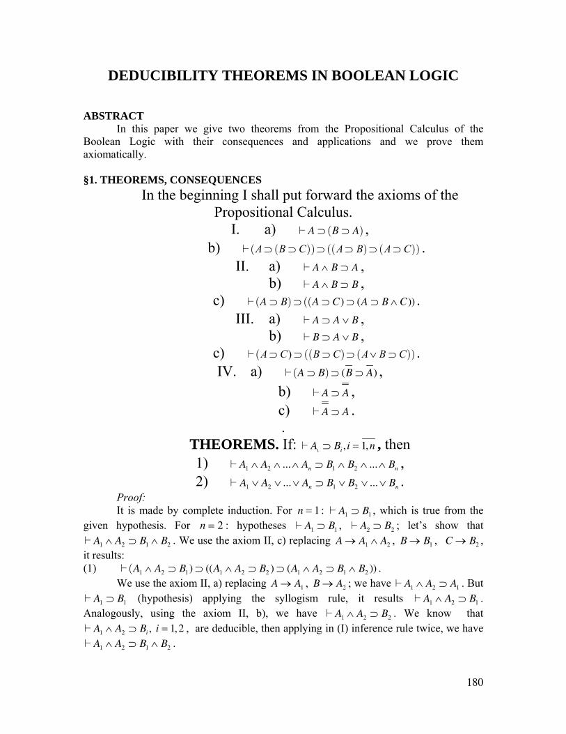
180
DEDUCIBILITY THEOREMS IN BOOLEAN LOGIC
ABSTRACT In this paper we give two theorems from the Propositional Calculus of the Boolean Logic with their consequences and applications and we prove them axiomatically. §1. THEOREMS, CONSEQUENCES
In the beginning I shall put forward the axioms of the Propositional Calculus.
I. a) A ⊃ (B ⊃ A) , b) A B C A B A C⊃ ⊃ ⊃ ⊃ ⊃ ⊃ ( ( )) (( ) ( )) .
II. a) A ∧ B ⊃ A , b) A ∧ B ⊃ B ,
c) (A ⊃ B) ⊃ ((A ⊃ C) ⊃ (A ⊃ B ∧ C)) . III. a) A ⊃ A ∨ B , b) B ⊃ A ∨ B ,
c) )A C B C A B C⊃ ⊃ ⊃ ⊃ ∨ ⊃ ( (( ) ( )) . IV. a) (A ⊃ B) ⊃ (B ⊃ A) ,
b) A ⊃ A , c) A ⊃ A .
. THEOREMS. If: Aι ⊃ Bi , i = 1,n , then 1) A1 ∧ A2 ∧ ... ∧ An ⊃ B1 ∧ B2 ∧ ... ∧ Bn , 2) A1 ∨ A2 ∨ ... ∨ An ⊃ B1 ∨ B2 ∨ ... ∨ Bn .
Proof: It is made by complete induction. For n = 1 : A1 ⊃ B1 , which is true from the given hypothesis. For n = 2 : hypotheses A1 ⊃ B1 , A2 ⊃ B2 ; let’s show that
A1 ∧ A2 ⊃ B1 ∧ B2 . We use the axiom II, c) replacing A → A1 ∧ A2 , B → B1 , C → B2 , it results: (1) (A1 ∧ A2 ⊃ B1) ⊃ ((A1 ∧ A2 ⊃ B2 ) ⊃ (A1 ∧ A2 ⊃ B1 ∧ B2 )) . We use the axiom II, a) replacing A → A1 , B → A2 ; we have A1 ∧ A2 ⊃ A1 . But
A1 ⊃ B1 (hypothesis) applying the syllogism rule, it results A1 ∧ A2 ⊃ B1 . Analogously, using the axiom II, b), we have A1 ∧ A2 ⊃ B2 . We know that
A1 ∧ A2 ⊃ Bi , i = 1,2 , are deducible, then applying in (I) inference rule twice, we have
A1 ∧ A2 ⊃ B1 ∧ B2 .
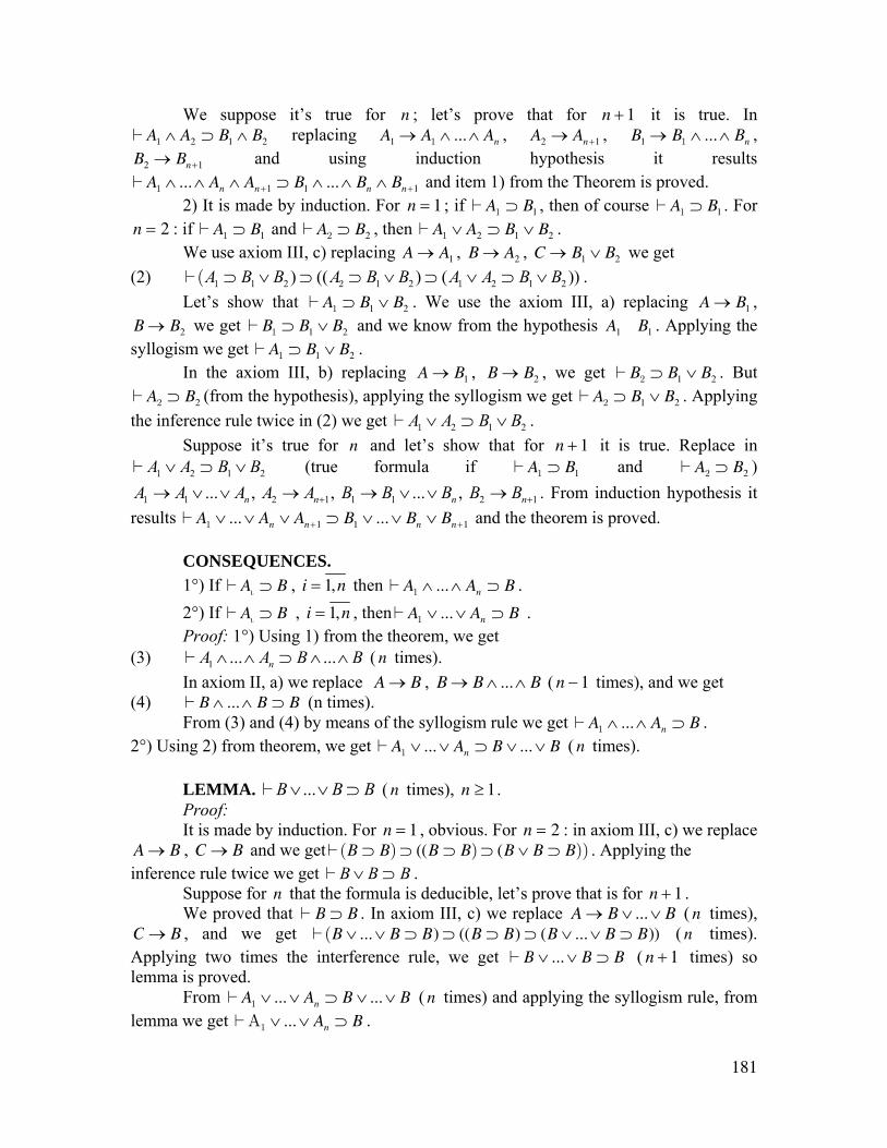
181
We suppose it’s true for n ; let’s prove that for n + 1 it is true. In A1 ∧ A2 ⊃ B1 ∧ B2 replacing A1 → A1 ∧ ... ∧ An , A2 → An+1 , B1 → B1 ∧ ... ∧ Bn , B2 → Bn+1 and using induction hypothesis it results
A1 ∧ ... ∧ An ∧ An+1 ⊃ B1 ∧ ... ∧ Bn ∧ Bn+1 and item 1) from the Theorem is proved. 2) It is made by induction. For n = 1 ; if A1 ⊃ B1 , then of course A1 ⊃ B1 . For n = 2 : if A1 ⊃ B1 and A2 ⊃ B2 , then A1 ∨ A2 ⊃ B1 ∨ B2 . We use axiom III, c) replacing A → A1 , B → A2 , C → B1 ∨ B2 we get (2) 1 2 1 2 2 1 2) (( ) ( ))A B B A B B A A B B⊃ ∨ ⊃ ⊃ ∨ ⊃ ∨ ⊃ ∨1 2 1 ( . Let’s show that A1 ⊃ B1 ∨ B2 . We use the axiom III, a) replacing A → B1 , B → B2 we get B1 ⊃ B1 ∨ B2 and we know from the hypothesis A1 B1 . Applying the syllogism we get A1 ⊃ B1 ∨ B2 . In the axiom III, b) replacing A → B1 , B → B2 , we get B2 ⊃ B1 ∨ B2 . But
A2 ⊃ B2 (from the hypothesis), applying the syllogism we get A2 ⊃ B1 ∨ B2 . Applying the inference rule twice in (2) we get 2 1 2A A B B∨ ⊃ ∨1 . Suppose it’s true for n and let’s show that for n + 1 it is true. Replace in
2 1 2A A B B∨ ⊃ ∨1 (true formula if A1 ⊃ B1 and A2 ⊃ B2 )
1 2 1 1 1 2 1... , , ... , n n n nA A A A A B B B B B+ +→ ∨ ∨ → → ∨ ∨ →1 . From induction hypothesis it results A1 ∨ ... ∨ An ∨ An+1 ⊃ B1 ∨ ... ∨ Bn ∨ Bn+1 and the theorem is proved. CONSEQUENCES. 1°) If Aι ⊃ B , i = 1,n then A1 ∧ ... ∧ An ⊃ B . 2°) If Aι ⊃ B , i = 1,n , then A1 ∨ ... ∨ An ⊃ B . Proof: 1°) Using 1) from the theorem, we get (3) 1 ... ...nA A B B∧ ∧ ⊃ ∧ ∧ ( n times). In axiom II, a) we replace A → B , B → B ∧ ...∧ B ( n − 1 times), and we get (4) B ∧ ... ∧ B ⊃ B (n times).
From (3) and (4) by means of the syllogism rule we get A1 ∧ ... ∧ An ⊃ B . 2°) Using 2) from theorem, we get A1 ∨ ... ∨ An ⊃ B ∨ ... ∨ B ( n times).
LEMMA. ...B B B∨ ∨ ⊃ ( n times), n ≥ 1. Proof:
It is made by induction. For n = 1 , obvious. For n = 2 : in axiom III, c) we replace A → B , C → B and we get (B ⊃ B) ⊃ ((B ⊃ B) ⊃ (B ∨ B ⊃ B)) . Applying the inference rule twice we get B B B∨ ⊃ .
Suppose for n that the formula is deducible, let’s prove that is for n + 1 . We proved that B ⊃ B . In axiom III, c) we replace A → B ∨ ...∨ B ( n times),
C → B , and we get (B ∨ ... ∨ B ⊃ B) ⊃ ((B ⊃ B) ⊃ (B ∨ ... ∨ B ⊃ B)) ( n times). Applying two times the interference rule, we get B ∨ ... ∨ B ⊃ B ( n + 1 times) so lemma is proved.
From A1 ∨ ... ∨ An ⊃ B ∨ ... ∨ B ( n times) and applying the syllogism rule, from lemma we get Α1 ∨ ... ∨ An ⊃ B .
182
3°) A ∧ ... ∧ A ⊃ A ( n times) 4°) A ∨ ... ∨ A ⊃ A ( n times).
Previously we proved, replacing in Consequence 1°) and 2°), B → A . Analogously, the consequences are proven:
5°) If A ⊃ Bi , i = 1,n , then A ⊃ B1 ∧ ... ∧ Bn . 6°) If A ⊃ Bi , i = 1,n , then A ⊃ B1 ∨ ... ∨ Bn . Analogously, 7°) A ⊃ A ∧ ... ∧ A ( n times) 8°) A ⊃ A ∨ ... ∨ A ( n times) 9°) A1 ∧ ... ∧ An ⊃ A1 ∨ ... ∨ An . Proof:
Method I. It is initially proved by induction: A1 ∧ ... ∧ An ⊃ Ai , i = 1,n and 2) is applied from the Theorem. Method II. It is proven by induction that: Aι ⊃ A1 ∧ ... ∧ An , i = 1,n and then 1) is applied from the Theorem.
10°) If Aι ⊃ Bi , i = 1,n , then A1 ∧ ... ∧ An ⊃ B1 ∨ ... ∨ Bn . Proof:
Method I. Using 1) from the Theorem, it results: (5) A1 ∧ ... ∧ An ⊃ B1 ∧ ... ∧ Bn We apply the Consequence 9°) where we replace Ai → Bi , i = 1,n and results: (6) B1 ∧ ... ∧ Bn ⊃ B1 ∨ ... ∨ Bn . From (5) and (6), applying the syllogism rule we get 10°). Method II. We firstly use the Consequence 9°) and then 2) from the Theorem and so we obtain the Consequence 10°).
§2. APPLICATIONS AND REMARKS ON THEOREMS The theorems are used in order to prove the formulae of the shape:
A1 ∧ ...∧ Ap ⊃ B1 ∧ ...∧ Br
A1 ∨ ...∨ Ap ⊃ B1 ∨ ...∨ Br , where p,r ∈N∗ It is proven that Aι ⊃ Bj , i.e.
∀i ∈1, p , ∃j0 ∈1,r , j0 = j0 (i) , Aι ⊃ Bj0
and ∀j ∈1,r , ∃i0 ∈1, p , i0 = i0 ( j) , Aι0
⊃ Bj . EXAMPLES: The following formulas are deducible: (i) A ⊃ (A ∨ B) ∧ (B ⊃ A) , (ii) (A ∧ B) ∨ C ⊃ A ∨ B ∨ C , (iii) A ∧ C ⊃ A ∨ C . Solution:
(i) We have A ⊃ A ∨ B and A ⊃ (B ⊃ A) (axiom III, a) and I, a)) and according to 1) from Theorem it results (i).
183
(ii) From A ⊃ (B ⊃ A) , A ∧ B ⊃ B , C C⊃ and Theorem 1), we have (ii).
(iii) Method I. From A ∧ C ⊃ A , A ∧ C ⊃ C and Theorem 2). Method II. From A ⊃ A ∨ C , C A C⊃ ∨ and using Theorem 1).
REMARKS. 1) The reciprocals of Theorem 1) and 2) are not always true. a) Counter-example for Theorem 1). The formula A ∧ B ⊃ A ∧ A is deducible
from axiom II, a), A A A∧ ⊃ (Consequence 7°) and the syllogism rule. But A ⊃ A for all A, that the formula B ⊃ A is not deducible, so the reciprocal of the Theorem 1) is false. Counter-example for Theorem 2). The formula A ∨ A ⊃ A ∨ B is deducible from Lemma, axiom III, a) and applying the syllogism rule. But A ⊃ A for all A, that the formula A ⊃ B is not deducible, so the reciprocal of Theorem 2) is false. 2) The reciprocals of Theorem 1) and 2) are not always true. Counter-examples:
a) for Theorem 1): A ⊃ A and B A⊃/ results that A ∧ B ⊃ A ∧ A so the reciprocal of Theorem 1) is false.
b) for Theorem 2): A ⊃ A and A B⊃/ results that A ∨ A ⊃ A ∨ B so the reciprocal of Theorem 2) is false.
REFERENCES:
[1] P. S. NOVOKOV. Elemente de logică matematică, Editura Ştiinţifică,
Bucureşti, 1966. [2] H. FREUDENTHAL, Limbajul logicii matematice, Editura Tehnică,
Bucureşti, 1973. UNIVERSITATEA DIN CRAIOVA Facultatea de tiinte Exacte 24.10.1979 [Published in “An. Univ. Timişoara”, Seria Şt. Matematice, Vol. XVII, Fasc. 2,
1979, pp. 164-8.]
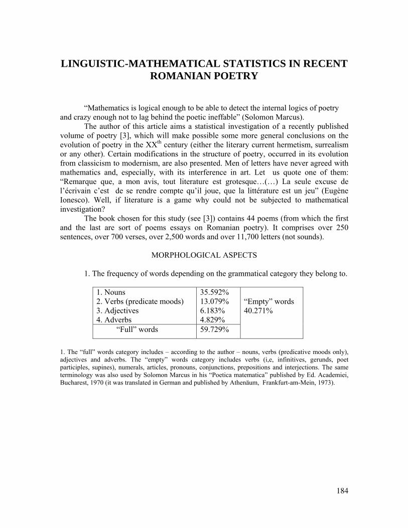
184
LINGUISTIC-MATHEMATICAL STATISTICS IN RECENT
ROMANIAN POETRY
“Mathematics is logical enough to be able to detect the internal logics of poetry and crazy enough not to lag behind the poetic ineffable” (Solomon Marcus). The author of this article aims a statistical investigation of a recently published volume of poetry [3], which will make possible some more general conclusions on the evolution of poetry in the XXth century (either the literary current hermetism, surrealism or any other). Certain modifications in the structure of poetry, occurred in its evolution from classicism to modernism, are also presented. Men of letters have never agreed with mathematics and, especially, with its interference in art. Let us quote one of them: “Remarque que, a mon avis, tout literature est grotesque…(…) La seule excuse de l’écrivain c’est de se rendre compte qu’il joue, que la littérature est un jeu” (Eugène Ionesco). Well, if literature is a game why could not be subjected to mathematical investigation? The book chosen for this study (see [3]) contains 44 poems (from which the first and the last are sort of poems essays on Romanian poetry). It comprises over 250 sentences, over 700 verses, over 2,500 words and over 11,700 letters (not sounds).
MORPHOLOGICAL ASPECTS 1. The frequency of words depending on the grammatical category they belong to.
1. Nouns 2. Verbs (predicate moods) 3. Adjectives 4. Adverbs
35.592% 13.079% 6.183% 4.829%
“Full” words 59.729%
“Empty” words 40.271%
1. The “full” words category includes – according to the author – nouns, verbs (predicative moods only), adjectives and adverbs. The “empty” words category includes verbs (i,e, infinitives, gerunds, poet participles, supines), numerals, articles, pronouns, conjunctions, prepositions and interjections. The same terminology was also used by Solomon Marcus in his “Poetica matematica” published by Ed. Academiei, Bucharest, 1970 (it was translated in German and published by Athenäum, Frankfurt-am-Mein, 1973).
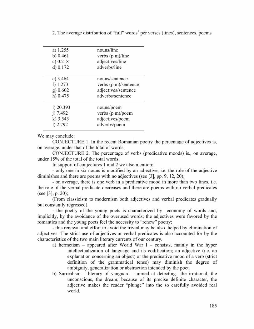
185
2. The average distribution of “full” words1 per verses (lines), sentences, poems a) 1.255 nouns/line b) 0.461 verbs (p.m)/line
c) 0.218 adjectives/line d) 0.172 adverbs/line e) 3.464 nouns/sentence f) 1.273 verbs (p.m)/sentence g) 0.602 adjectives/sentence h) 0.475 adverbs/sentence i) 20.393 nouns/poem j) 7.492 verbs (p.m)/poem k) 3.543 adjectives/poem l) 2.792 adverbs/poem We may conclude: CONJECTURE 1. In the recent Romanian poetry the percentage of adjectives is, on average, under that of the total of words. CONJECTURE 2. The percentage of verbs (predicative moods) is., on average, under 15% of the total of the total words.
In support of conjectures 1 and 2 we also mention: - only one in six nouns is modified by an adjective, i.e. the role of the adjective
diminishes and there are poems with no adjectives (see [3], pp. 9, 12, 20); - on average, there is one verb in a predicative mood in more than two lines, i.e.
the role of the verbal predicate decreases and there are poems with no verbal predicates (see [3], p. 20);
(From classicism to modernism both adjectives and verbal predicates gradually but constantly regressed).
- the poetry of the young poets is characterized by economy of words and, implicitly, by the avoidance of the overused words; the adjectives were favored by the romantics and the young poets feel the necessity to “renew” poetry;
- this renewal and effort to avoid the trivial may be also helped by elimination of adjectives. The strict use of adjectives or verbal predicates is also accounted for by the characteristics of the two main literary currents of our century.
a) hermetism – appeared after World War I – consists, mainly in the hyper intellectualization of language and its codification; an adjective (i.e. an explanation concerning an object) or the predicative mood of a verb (strict definition of the grammatical tense) may diminish the degree of ambiguity, generalization or abstraction intended by the poet.
b) Surrealism – literary of vanguard – aimed at detecting the irrational, the unconscious, the dream; because of its precise definite character, the adjective makes the reader “plunge” into the so carefully avoided real world.
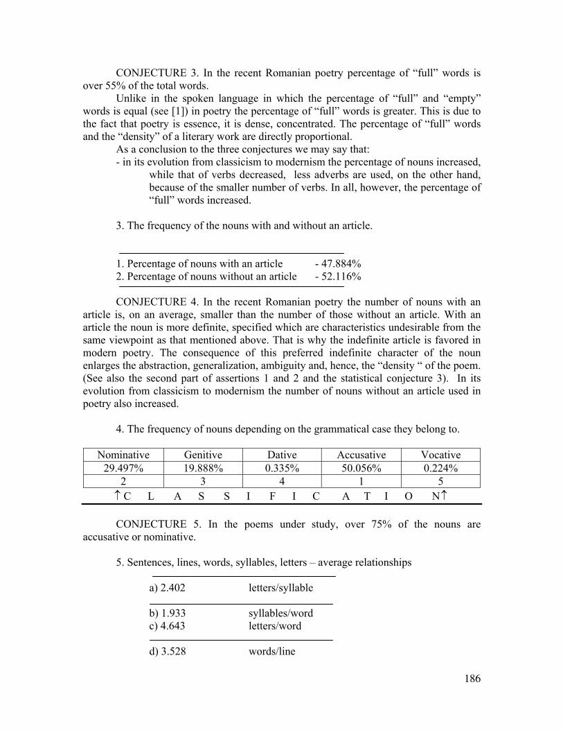
186
CONJECTURE 3. In the recent Romanian poetry percentage of “full” words is over 55% of the total words.
Unlike in the spoken language in which the percentage of “full” and “empty” words is equal (see [1]) in poetry the percentage of “full” words is greater. This is due to the fact that poetry is essence, it is dense, concentrated. The percentage of “full” words and the “density” of a literary work are directly proportional.
As a conclusion to the three conjectures we may say that: - in its evolution from classicism to modernism the percentage of nouns increased,
while that of verbs decreased, less adverbs are used, on the other hand, because of the smaller number of verbs. In all, however, the percentage of “full” words increased.
3. The frequency of the nouns with and without an article.
1. Percentage of nouns with an article - 47.884% 2. Percentage of nouns without an article - 52.116%
CONJECTURE 4. In the recent Romanian poetry the number of nouns with an article is, on an average, smaller than the number of those without an article. With an article the noun is more definite, specified which are characteristics undesirable from the same viewpoint as that mentioned above. That is why the indefinite article is favored in modern poetry. The consequence of this preferred indefinite character of the noun enlarges the abstraction, generalization, ambiguity and, hence, the “density “ of the poem. (See also the second part of assertions 1 and 2 and the statistical conjecture 3). In its evolution from classicism to modernism the number of nouns without an article used in poetry also increased. 4. The frequency of nouns depending on the grammatical case they belong to.
Nominative Genitive Dative Accusative Vocative 29.497% 19.888% 0.335% 50.056% 0.224%
2 3 4 1 5 ↑ C L A S S I F I C A T I O N↑
CONJECTURE 5. In the poems under study, over 75% of the nouns are
accusative or nominative.
5. Sentences, lines, words, syllables, letters – average relationships a) 2.402 letters/syllable
b) 1.933 syllables/word
c) 4.643 letters/word d) 3.528 words/line
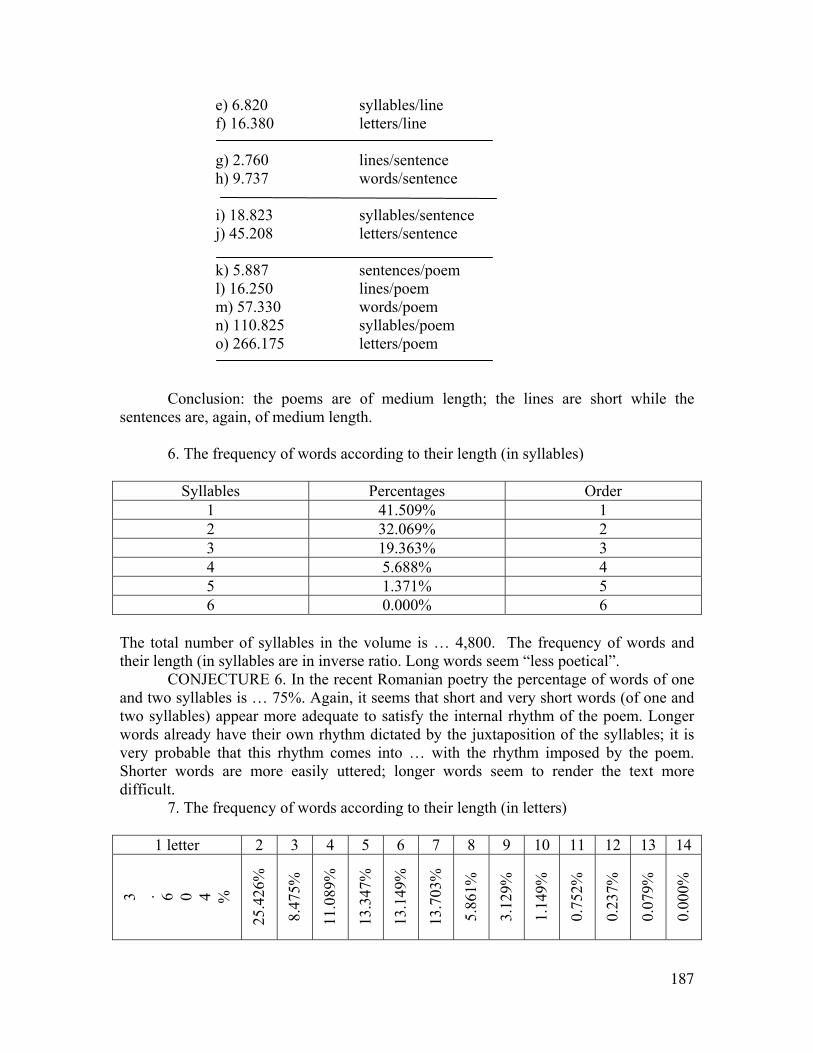
187
e) 6.820 syllables/line f) 16.380 letters/line g) 2.760 lines/sentence
h) 9.737 words/sentence i) 18.823 syllables/sentence j) 45.208 letters/sentence k) 5.887 sentences/poem l) 16.250 lines/poem m) 57.330 words/poem n) 110.825 syllables/poem o) 266.175 letters/poem
Conclusion: the poems are of medium length; the lines are short while the sentences are, again, of medium length. 6. The frequency of words according to their length (in syllables)
Syllables Percentages Order 1 41.509% 1 2 32.069% 2 3 19.363% 3 4 5.688% 4 5 1.371% 5 6 0.000% 6
The total number of syllables in the volume is … 4,800. The frequency of words and their length (in syllables are in inverse ratio. Long words seem “less poetical”. CONJECTURE 6. In the recent Romanian poetry the percentage of words of one and two syllables is … 75%. Again, it seems that short and very short words (of one and two syllables) appear more adequate to satisfy the internal rhythm of the poem. Longer words already have their own rhythm dictated by the juxtaposition of the syllables; it is very probable that this rhythm comes into … with the rhythm imposed by the poem. Shorter words are more easily uttered; longer words seem to render the text more difficult. 7. The frequency of words according to their length (in letters)
1 letter 2 3 4 5 6 7 8 9 10 11 12 13 14
3 . 6 0 4 %
25.4
26%
8.47
5%
11.0
89%
13.3
47%
13.1
49%
13.7
03%
5.86
1%
3.12
9%
1.14
9%
0.75
2%
0.23
7%
0.07
9%
0.00
0%
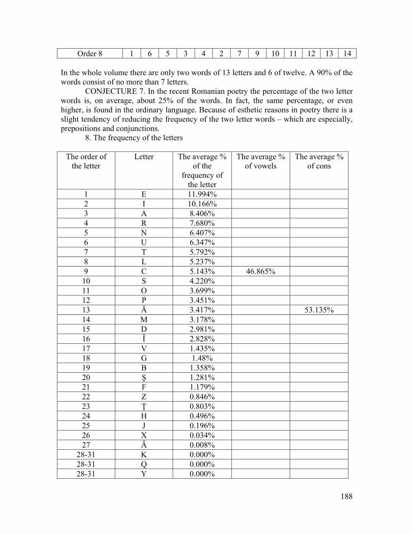
188
Order 8 1 6 5 3 4 2 7 9 10 11 12 13 14 In the whole volume there are only two words of 13 letters and 6 of twelve. A 90% of the words consist of no more than 7 letters. CONJECTURE 7. In the recent Romanian poetry the percentage of the two letter words is, on average, about 25% of the words. In fact, the same percentage, or even higher, is found in the ordinary language. Because of esthetic reasons in poetry there is a slight tendency of reducing the frequency of the two letter words – which are especially, prepositions and conjunctions. 8. The frequency of the letters
The order of the letter
Letter The average % of the
frequency of the letter
The average % of vowels
The average % of cons
1 E 11.994% 2 I 10.166% 3 A 8.406% 4 R 7.680% 5 N 6.407% 6 U 6.347% 7 T 5.792% 8 L 5.237% 9 C 5.143% 46.865% 10 S 4.220% 11 O 3.699% 12 P 3.451% 13 Ă 3.417% 53.135% 14 M 3.178% 15 D 2.981% 16 Î 2.828% 17 V 1.435% 18 G 1.48% 19 B 1.358% 20 Ş 1.281% 21 F 1.179% 22 Z 0.846% 23 Ţ 0.803% 24 H 0.496% 25 J 0.196% 26 X 0.034% 27 Ă 0.008%
28-31 K 0.000% 28-31 Q 0.000% 28-31 Y 0.000%
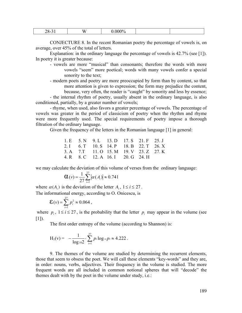
189
28-31 W 0.000% CONJECTURE 8. In the recent Romanian poetry the percentage of vowels is, on average, over 45% of the total of letters. Explanation: in the ordinary language the percentage of vowels is 42.7% (see [1]). In poetry it is greater because:
- vowels are more “musical” than consonants; therefore the words with more vowels “seem” more poetical; words with many vowels confer a special sonority to the text;
- modern poets and poetry are more preoccupied by form than by content, so that more attention is given to expression; the form may prejudice the content, because, very often, the reader is “caught” by sonority and less by essence;
- the internal rhythm of poetry, usually absent in the ordinary language, is also conditioned, partially, by a greater number of vowels;
- rhyme, when used, also favors a greater percentage of vowels. The percentage of vowels was greater in the period of classicism of poetry when the rhythm and rhyme were more frequently used. The special requirements of poetry impose a thorough filtration of the ordinary language.
Given the frequency of the letters in the Romanian language [1] in general:
1. E 5. N 9. L 13. D 17. S 21. F 25. J 2. I 6. T 10. S 14. P 18. B 22. T 26. X 3. A 7.T 11. O 15. M 19. V 23. Z 27. K 4. R 8. C 12. A 16. I 20. G 24. H
we may calculate the deviation of this volume of verses from the ordinary language:
α 27
1
1( ) ( ) 0.74127 i
i
v Aα=
= ≈∑
where α (Ai ) is the deviation of the letter Ai , 1 ≤ i ≤ 27 . The informational energy, according to O. Onicescu, is
ε 272
1( ) 0.064i
iv p
=
= ≈∑ ,
where pi , 1 ≤ i ≤ 27 , is the probability that the letter pi may appear in the volume (see [1]). The first order entropy of the volume (according to Shannon) is:
H1(v) = ∑=
≈⋅−27
110222.4log
2log1
10
i
ii pp .
9. The themes of the volume are studied by determining the recurrent elements, those that seem to obsess the poet. We will call these elements “key-words” and they are, in order: nouns, verbs, adjectives. Their frequency in the volume is studied. The more frequent words are all included in common notional spheres that will “decode” the themes dealt with by the poet in the volume under study, i.e.:
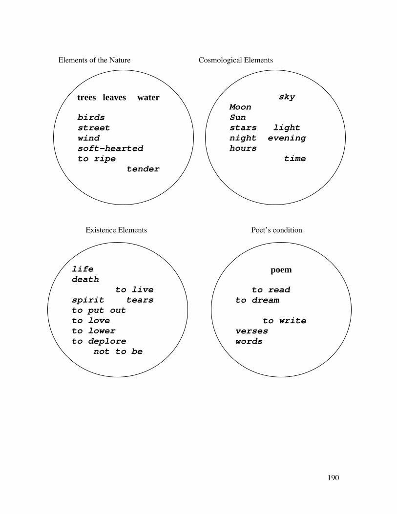
190
Elements of the Nature Cosmological Elements Existence Elements Poet’s condition
trees leaves water birds street wind soft-hearted to ripe tender
sky Moon Sun stars light night evening hours time
life death to live spirit tears to put out to love to lower to deplore not to be
poem to read to dream to write verses words
191
These 33 key-words (together with their synonyms) confer certain pastoral note (this was noticed by Constantin Matei, the newspaper ”Înainte”, Craiova), cosmological (Constantin M. Popa), existentialist nuances (Aureliu Goci, “Luceafarul”, Bucharest); the preoccupation of the poet for the condition of the poet and society (Ion Pachia Tatomirescu, Craiova) is also revealed by the frequent use of certain suggestive words. Of all the words, 33 key-words together with their synonyms have the greatest frequency in the volume. 10. The frequency of words and phrases strongly deviated from the “normal”, i.e. the rules of the literary language are about 1.980 of the total of words. (We mean expressions like: “state of self”, “very near myself”, “it is raining at plus infinite” or words like “nontime”, etc. (see [3], pp. 9, 29, 40, 31). CONJECTURE 9. In the recent Romanian poetry the percentage of words and phrases that strongly deviated from the “normal” of the ordinary language, as well as the rules of the literary language, is slightly over 1. This fact may be accounted for by:
- content seems less important; poets are more concerned with form; - poets invent words and expressions to be able to better reveal their feelings
and emotions; - the association of antonyms may give birth to constructions that, somehow
“violate” the normal; - poetry is, in fact, destined to break the rules and rebel against the ordinary fact
(if, this right is denied, any newspaper article could be called poetry). “In art” said Voltaire, “rules are only meant to be broken”. In its evaluation from classicism to modernism the percentage of such abnormal
words and constructions increased, starting, in fact from zero. Modern literary currents favor the appearance of them.
REFERENCES [1] Marcus, Solomon – “Poetica matematică” – Ed. Academiei, Bucharest, 1970
(translated into German, Athenäum, Frankfurt-am-Mein, 1973). [2] Marcus, Solomon, Edmond Nicolau, Sorin Stati – “Introducere în lingvistica
matematică”, Bucharest, 1966 (translated in Italian, Patron, Bologna, 1971 and in Spanish, Teide, Barcelona, 1978).
[3] Florentin, Ovidiu – “Formule pentru spirit”, Ed. Litera, Bucharest, 1981 (Translated in French, les Editions Express, Fès, Morocco, 1983); modern poems.
[4] Smarandache, Florentin – “A mathematical linguistic approach to Rebus” – article published in “Revue roumain de linguistique”, tome XXVIII, 1983, collection “Cahiers de linguistique théorique et appliquée”, tome XX, 1983, No. 1, pp. 67-76.
[Editions Scientifiques, Casablanca, Morocco, 1984]
192
A MATHEMATICAL LINGUISTIC APPROACH TO REBUS
INTRODUCTION
The aim of this paper is the investigation of some combinatorial aspects of written language, within the framework determined by the well-known game of crossword puzzles. Various types of probabilistic regularities appearing in such puzzles reveal some hidden, not well-known restrictions operating in the field of natural languages. Most of the restrictions of this type are similar in each natural language. Our direct concern will be the Romanian language. Our research may have some relevance for the phono-statistics of Romanian. The distribution of phonemes and letters is established for a corpus of a deviant morphological structure with respect to the standard language. Another aspect of our research may be related to the so-called tabular reading in poetry. The correlation horizontal-vertical considered in the first part of the paper offers some suggestions concerning a bi-dimensional investigation of the poetic sing. Our investigation is concerned with the Romanian crossword puzzles published in [4]. Various concepts concerning crossword puzzles are borrowed from N. Andrei [3]. Mathematical linguistic concepts are borrowed from S. Marcus [1], and S. Marcus, E. Nicolau, S. Stati [2].
SECTION 1. THE GRID
§1. MATHEMATICAL RESEARCHES ON GRIDS It is known that a word in a grid is limited on the left and right side either by a black point or by a grid final border. We will take into account the words consisting of one letter (though they are not clued in the Rebus), and those of two (even they have no sense (e.g. NT, RU,…)), three or more letters – even they represent that category of rare words (foreign localities, rivers, etc., abbreviations, etc., which are not found in the Romanian Language Dictionary (see [3], pp. 82-307 (“Rebus glossary”)).
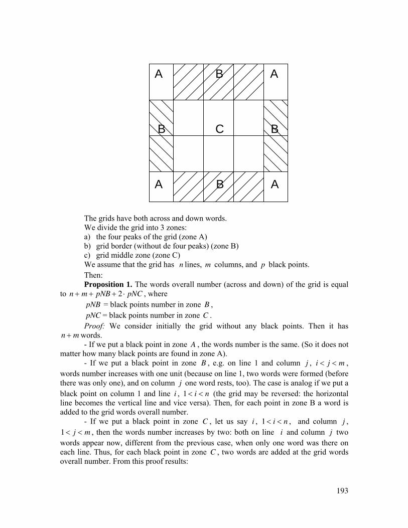
193
The grids have both across and down words. We divide the grid into 3 zones:
a) the four peaks of the grid (zone A) b) grid border (without de four peaks) (zone B) c) grid middle zone (zone C) We assume that the grid has n lines, m columns, and p black points. Then: Proposition 1. The words overall number (across and down) of the grid is equal
to n + m + pNB + 2 ⋅ pNC , where pNB = black points number in zone B ,
pNC = black points number in zone C . Proof: We consider initially the grid without any black points. Then it has n + m words.
- If we put a black point in zone A , the words number is the same. (So it does not matter how many black points are found in zone A).
- If we put a black point in zone B , e.g. on line 1 and column j , i < j < m , words number increases with one unit (because on line 1, two words were formed (before there was only one), and on column j one word rests, too). The case is analog if we put a black point on column 1 and line i , 1 < i < n (the grid may be reversed: the horizontal line becomes the vertical line and vice versa). Then, for each point in zone B a word is added to the grid words overall number.
- If we put a black point in zone C , let us say i , 1 < i < n , and column j , 1 < j < m , then the words number increases by two: both on line i and column j two words appear now, different from the previous case, when only one word was there on each line. Thus, for each black point in zone C , two words are added at the grid words overall number. From this proof results:
A B A B C B
A B A
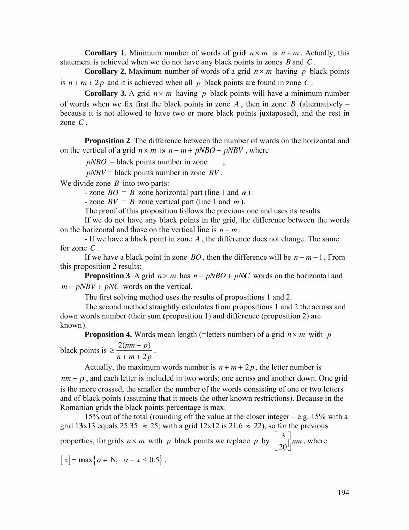
194
Corollary 1. Minimum number of words of grid n × m is n + m . Actually, this statement is achieved when we do not have any black points in zones B and C .
Corollary 2. Maximum number of words of a grid n × m having p black points is n + m + 2 p and it is achieved when all p black points are found in zone C .
Corollary 3. A grid n × m having p black points will have a minimum number of words when we fix first the black points in zone A , then in zone B (alternatively – because it is not allowed to have two or more black points juxtaposed), and the rest in zone C .
Proposition 2. The difference between the number of words on the horizontal and
on the vertical of a grid n × m is n − m + pNBO − pNBV , where pNBO = black points number in zone ,
pNBV = black points number in zone BV . We divide zone B into two parts:
- zone BO = B zone horizontal part (line 1 and n ) - zone BV = B zone vertical part (line 1 and m ). The proof of this proposition follows the previous one and uses its results. If we do not have any black points in the grid, the difference between the words
on the horizontal and those on the vertical line is n − m . - If we have a black point in zone A , the difference does not change. The same
for zone C . If we have a black point in zone BO , then the difference will be n − m − 1. From
this proposition 2 results: Proposition 3. A grid n × m has n + pNBO + pNC words on the horizontal and
m + pNBV + pNC words on the vertical. The first solving method uses the results of propositions 1 and 2. The second method straightly calculates from propositions 1 and 2 the across and
down words number (their sum (proposition 1) and difference (proposition 2) are known).
Proposition 4. Words mean length (=letters number) of a grid n × m with p
black points is ≥2(nm − p)
n + m + 2 p.
Actually, the maximum words number is n + m + 2 p , the letter number is nm − p , and each letter is included in two words: one across and another down. One grid is the more crossed, the smaller the number of the words consisting of one or two letters and of black points (assuming that it meets the other known restrictions). Because in the Romanian grids the black points percentage is max.
15% out of the total (rounding off the value at the closer integer – e.g. 15% with a grid 13x13 equals 25.35 ≈ 25; with a grid 12x12 is 21.6 ≈ 22), so for the previous
properties, for grids n × m with p black points we replace p by 3
20⎡⎣⎢
⎤⎦⎥
nm , where
[ ] { }max 0.5x xα α= ∈ Ν, − ≤ .
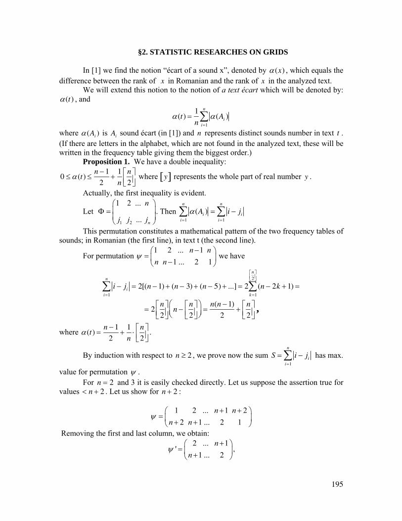
195
§2. STATISTIC RESEARCHES ON GRIDS In [1] we find the notion “écart of a sound x”, denoted by α(x) , which equals the
difference between the rank of x in Romanian and the rank of x in the analyzed text. We will extend this notion to the notion of a text écart which will be denoted by:
α(t) , and
α(t) =1
nα(Ai )
i=1
n
∑
where α (Ai ) is Ai sound écart (in [1]) and n represents distinct sounds number in text t . (If there are letters in the alphabet, which are not found in the analyzed text, these will be written in the frequency table giving them the biggest order.)
Proposition 1. We have a double inequality:
0 ≤ α (t) ≤n − 1
2+
1
n
n
2⎡⎣⎢
⎤⎦⎥
where y[ ] represents the whole part of real number y .
Actually, the first inequality is evident.
Let 1 2
1 2 ...
... n
n
j j j
⎛ ⎞⎜ ⎟Φ =⎜ ⎟⎝ ⎠
. Then α(Ai )i=1
n
∑ = i − jii=1
n
∑
This permutation constitutes a mathematical pattern of the two frequency tables of sounds; in Romanian (the first line), in text t (the second line).
For permutation 1 2 ... 1
1 ... 2 1n n
n nψ
−⎛ ⎞= ⎜ ⎟−⎝ ⎠
we have
i − jii=1
n
∑ = 2[(n − 1) + (n − 3) + (n − 5) + ...] = 2 (n − 2k + 1) =k =1
n
2⎡⎣⎢
⎤⎦⎥
∑
= 2n
2⎡⎣⎢
⎤⎦⎥
n −n
2⎡⎣⎢
⎤⎦⎥
⎛⎝⎜
⎞⎠⎟
=n(n − 1)
2+
n
2⎡⎣⎢
⎤⎦⎥,
where α(t) =n − 1
2+
1
n⋅
n
2⎡⎣⎢
⎤⎦⎥
.
By induction with respect to n ≥ 2 , we prove now the sum S = i − jii=1
n
∑ has max.
value for permutation ψ . For n = 2 and 3 it is easily checked directly. Let us suppose the assertion true for values < n + 2 . Let us show for n + 2 :
1 2 ... 1 22 1 ... 2 1
n nn n
ψ+ +⎛ ⎞
= ⎜ ⎟+ +⎝ ⎠
Removing the first and last column, we obtain: 2 ... 1
'1 ... 2
nn
ψ+⎛ ⎞
= ⎜ ⎟+⎝ ⎠,
196
which is a permutation of n elements and for which S will have the same value as for permutation
1 ... "
... 1n
nψ
⎛ ⎞= ⎜ ⎟
⎝ ⎠,
i.e. max. value ( "ψ was obtained from ψ ' by diminishing each element by one).
The permutation of 2 elements 1 2
2 1n
nη
+⎛ ⎞= ⎜ ⎟+⎝ ⎠
gives maximum value for S .
But ψ is obtained from ψ ' and η ;
{ }'( ), if 1, 2( )
( ), otherwise i i n
ii
ψψ
η∉ +⎧⎪= ⎨
⎪⎩
Remark : The bigger one text écart, the bigger the “angle of deviation” from the usual language. It would be interesting to calculate, for example, the écart of a poem. Then the notion of écart could be extended even more:
a) the écart of a word being equal to the difference between word order in language and word order in the text;
b) the écart of a text (ref. words):
αc (t) =1
nαc (ai )
i=1
n
∑ ,
where α c (ai ) is word ai écart, and n - distinct words number in the text t .
*
We give below some rebus statistic data. By examining 150 grids [4] we obtain the following results:
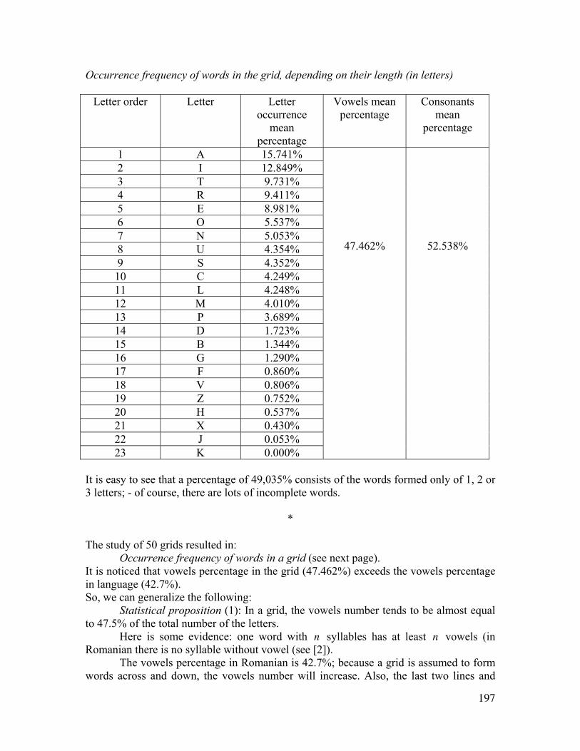
197
Occurrence frequency of words in the grid, depending on their length (in letters)
Letter order Letter Letter occurrence
mean percentage
Vowels mean percentage
Consonants mean
percentage
1 A 15.741% 2 I 12.849% 3 T 9.731% 4 R 9.411% 5 E 8.981% 6 O 5.537% 7 N 5.053% 8 U 4.354% 9 S 4.352% 10 C 4.249% 11 L 4.248% 12 M 4.010% 13 P 3.689% 14 D 1.723% 15 B 1.344% 16 G 1.290% 17 F 0.860% 18 V 0.806% 19 Z 0.752% 20 H 0.537% 21 X 0.430% 22 J 0.053% 23 K 0.000%
47.462%
52.538%
It is easy to see that a percentage of 49,035% consists of the words formed only of 1, 2 or 3 letters; - of course, there are lots of incomplete words.
* The study of 50 grids resulted in: Occurrence frequency of words in a grid (see next page). It is noticed that vowels percentage in the grid (47.462%) exceeds the vowels percentage in language (42.7%). So, we can generalize the following: Statistical proposition (1): In a grid, the vowels number tends to be almost equal to 47.5% of the total number of the letters. Here is some evidence: one word with n syllables has at least n vowels (in Romanian there is no syllable without vowel (see [2]). The vowels percentage in Romanian is 42.7%; because a grid is assumed to form words across and down, the vowels number will increase. Also, the last two lines and
198
columns are endings of other words in the grid; thus they will usually have more vowels. When black points number decreases, vowels number will increase (in order to have an easier crossing, you need either more black points or more vowels) (A vowel has a bigger probability to enter in the contents of a word than a consonant.) Especially in “record grids” (see [3], pp. 33-48) the vowels and consonants alternation is noticed. Another criterion for estimating the grid value is the bigger deviation from this “statistical law” (the exception confirms the rule!): i.e. the smaller the vowel percentage in a grid, the bigger its value. Statistical proposition (2): Generally, the horizontal words number 73 equals the vertical one. Here is the following evidence: 100 classical grids were experimentally analyzed, in [4], getting the percentage of 49.932% horizontal words. Usually, the classical grids are square clues, the difference between the horizontal and vertical words being (see Proposition 2):
n m pNBO pNBV pNBO pNBV− + − = − . The difference between the black points number in zone BO and zone BV can not be too big ( 1, 2± ± and rarely ± 3 ). (Usually, there are not many black points in zone B, because it is not economical in crossing (see proof of Proposition 1)). Taking from [1] the following letters frequency in language:
1. E 5.N 9. L 13. P 17. G 21. J
2. I 6.T 10. S 14. M 18. F 22. X 3.A 7.U 11. O 15. B 19. Z 23. K 4.R 8.C 12. D 16. V 20. H
(because in the grid Ă, Â, Î , Ş, Ţ: are replaced by A: I: S: T, respectively, in the above order they were cancelled) the écart of the 150 grids becomes
23
1
1( ) ( ) 1.39123 i
i
g Aα α=
= ≈∑ ;
the entropy is:
23
1 10110
1 3.8652 i i
i
H p log plog =
= − ≈∑
and the informational energy (after O. Onicescu) is: 23
2
1
( ) 0.084ii
E g p=
= ≈∑
Examining 50 grids we obtain:
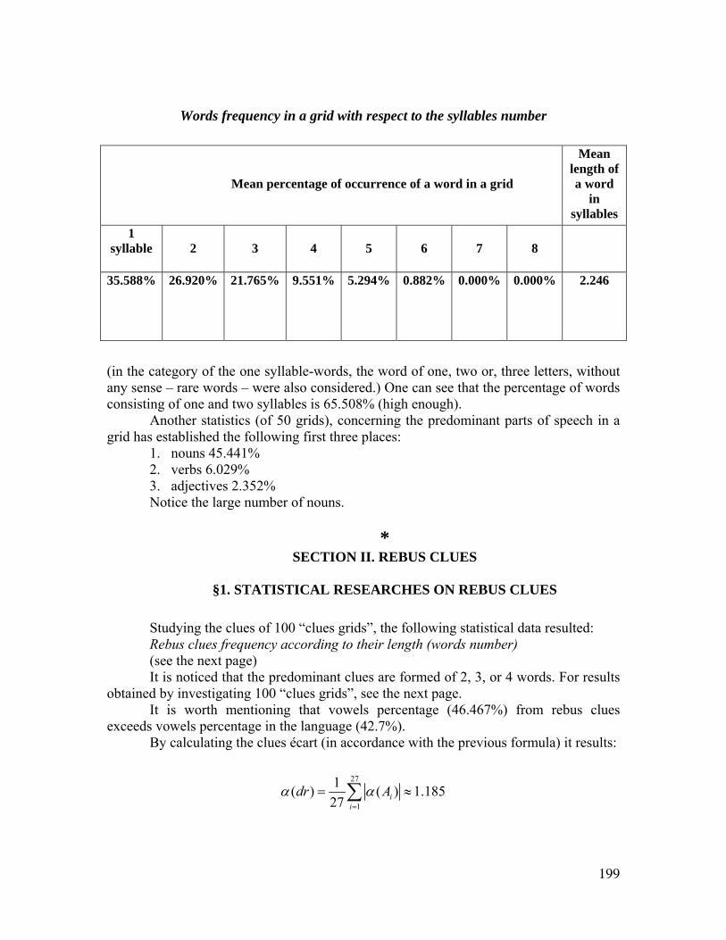
199
Words frequency in a grid with respect to the syllables number
Mean percentage of occurrence of a word in a grid
Mean length of a word
in syllables
1 syllable
2
3
4
5
6
7
8
35.588% 26.920% 21.765% 9.551% 5.294% 0.882% 0.000% 0.000% 2.246
(in the category of the one syllable-words, the word of one, two or, three letters, without any sense – rare words – were also considered.) One can see that the percentage of words consisting of one and two syllables is 65.508% (high enough). Another statistics (of 50 grids), concerning the predominant parts of speech in a grid has established the following first three places:
1. nouns 45.441% 2. verbs 6.029% 3. adjectives 2.352% Notice the large number of nouns.
* SECTION II. REBUS CLUES
§1. STATISTICAL RESEARCHES ON REBUS CLUES
Studying the clues of 100 “clues grids”, the following statistical data resulted: Rebus clues frequency according to their length (words number) (see the next page)
It is noticed that the predominant clues are formed of 2, 3, or 4 words. For results obtained by investigating 100 “clues grids”, see the next page.
It is worth mentioning that vowels percentage (46.467%) from rebus clues exceeds vowels percentage in the language (42.7%).
By calculating the clues écart (in accordance with the previous formula) it results:
27
1
1( ) ( ) 1.18527 i
idr Aα α
=
= ≈∑
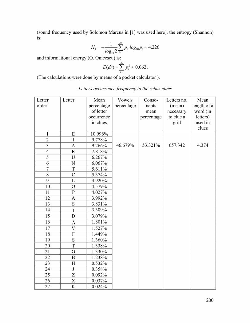
200
(sound frequency used by Solomon Marcus in [1] was used here), the entropy (Shannon) is:
27
1 10110
1 4.2262 i i
i
H p log plog =
= − ≈∑
and informational energy (O. Onicescu) is: 27
2
1
( ) 0.062ii
E dr p=
= ≈∑ .
(The calculations were done by means of a pocket calculator ).
Letters occurrence frequency in the rebus clues
Letter order
Letter Mean percentage
of letter occurrence
in clues
Vowels percentage
Conso- nants mean
percentage
Letters no. (mean)
necessary to clue a
grid
Mean length of a word (in letters) used in clues
1 E 10.996% 2 I 9.778% 3 A 9.266% 4 R 7.818% 5 U 6.267% 6 N 6.067% 7 T 5.611% 8 C 5.374% 9 L 4.920% 10 O 4.579% 11 P 4.027% 12 Ă 3.992% 13 S 3.831% 14 Î 3.309% 15 D 3.079% 16 Â 1.801% 17 V 1.527% 18 F 1.449% 19 Ş 1.360% 20 Ţ 1.338% 21 G 1.330% 22 B 1.238% 23 H 0.532% 24 J 0.358% 25 Z 0.092% 26 X 0.037% 27 K 0.024%
46.679%
53.321%
657.342
4.374
201
REFERENCES
[1] Marcus, Solomon – “Poetica matematica” – Ed. Academiei, Bucureşti,
1970 (German translation, Athenäum, Frankfurt am Mein, 1973). [2] Marcus, Solomon, Edmond Nicolau, S. Stati – Introducere în lingvistica
matematică, Bucureşti, 1966 (Italian translation, Patron, Bologna, 1971; Spanish translation, Teide, Barcelona, 1978).
[3] Andrei, Dr. N. – Îndreptar rebusist, Ed. Sport-Turism, Bucureşti, 1981. [4] “Rebus” magazine collection, Bucureşti, 1979-1982. The Craiova University Natural Sciences Department
[Published in “Review Roumaine de linguistique”, Tome XXVIII, 1983, “Cahiers de linguistique théorique et appliquée”, Bucharest, Tome XX, 1983, No. 1, pp. 67-76.]
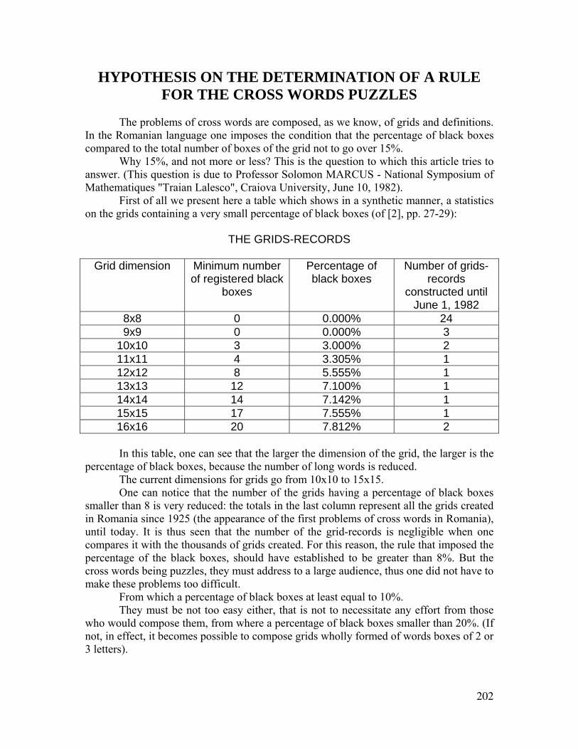
202
HYPOTHESIS ON THE DETERMINATION OF A RULE FOR THE CROSS WORDS PUZZLES
The problems of cross words are composed, as we know, of grids and definitions. In the Romanian language one imposes the condition that the percentage of black boxes compared to the total number of boxes of the grid not to go over 15%. Why 15%, and not more or less? This is the question to which this article tries to answer. (This question is due to Professor Solomon MARCUS - National Symposium of Mathematiques "Traian Lalesco", Craiova University, June 10, 1982). First of all we present here a table which shows in a synthetic manner, a statistics on the grids containing a very small percentage of black boxes (of [2], pp. 27-29):
THE GRIDS-RECORDS
Grid dimension Minimum number of registered black
boxes
Percentage of black boxes
Number of grids-records
constructed until June 1, 1982
8x8 0 0.000% 24 9x9 0 0.000% 3
10x10 3 3.000% 2 11x11 4 3.305% 1 12x12 8 5.555% 1 13x13 12 7.100% 1 14x14 14 7.142% 1 15x15 17 7.555% 1 16x16 20 7.812% 2
In this table, one can see that the larger the dimension of the grid, the larger is the percentage of black boxes, because the number of long words is reduced. The current dimensions for grids go from 10x10 to 15x15. One can notice that the number of the grids having a percentage of black boxes smaller than 8 is very reduced: the totals in the last column represent all the grids created in Romania since 1925 (the appearance of the first problems of cross words in Romania), until today. It is thus seen that the number of the grid-records is negligible when one compares it with the thousands of grids created. For this reason, the rule that imposed the percentage of the black boxes, should have established to be greater than 8%. But the cross words being puzzles, they must address to a large audience, thus one did not have to make these problems too difficult. From which a percentage of black boxes at least equal to 10%. They must be not too easy either, that is not to necessitate any effort from those who would compose them, from where a percentage of black boxes smaller than 20%. (If not, in effect, it becomes possible to compose grids wholly formed of words boxes of 2 or 3 letters).
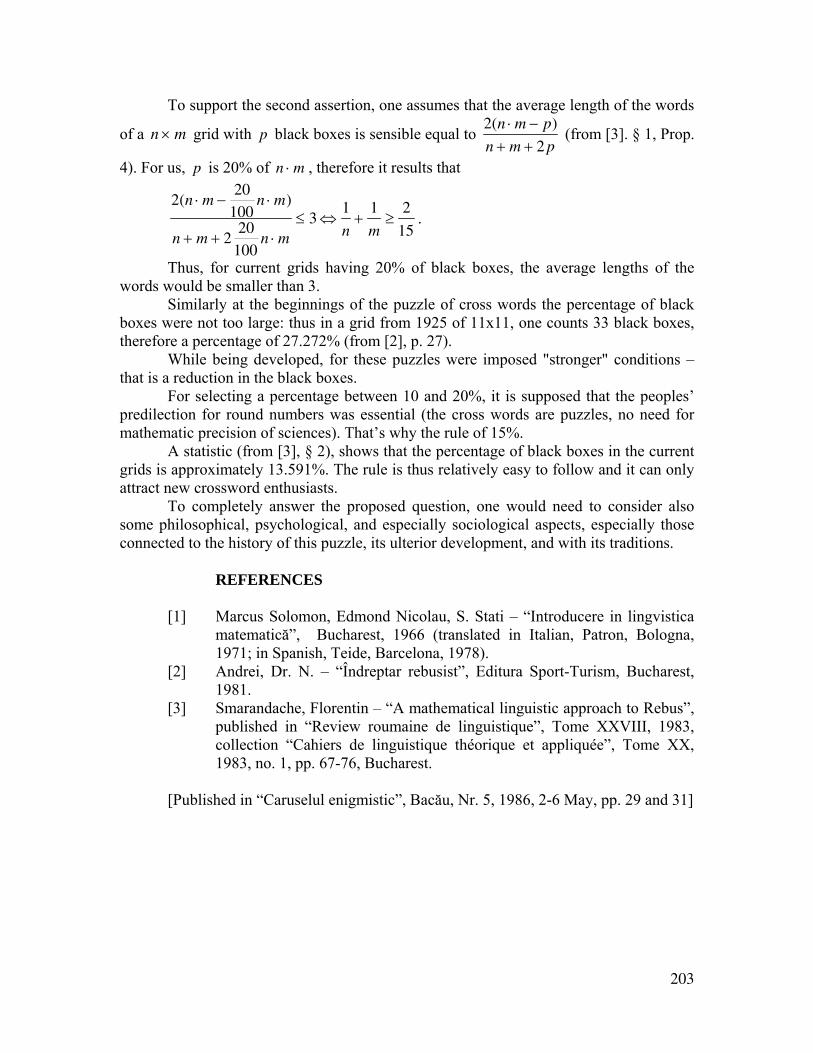
203
To support the second assertion, one assumes that the average length of the words
of a n × m grid with p black boxes is sensible equal to 2(n ⋅ m − p)
n + m + 2 p (from [3]. § 1, Prop.
4). For us, p is 20% of n ⋅ m , therefore it results that
2(n ⋅ m −
20
100n ⋅ m)
n + m + 220
100n ⋅ m
≤ 3 ⇔1
n+
1
m≥
2
15.
Thus, for current grids having 20% of black boxes, the average lengths of the words would be smaller than 3.
Similarly at the beginnings of the puzzle of cross words the percentage of black boxes were not too large: thus in a grid from 1925 of 11x11, one counts 33 black boxes, therefore a percentage of 27.272% (from [2], p. 27).
While being developed, for these puzzles were imposed "stronger" conditions – that is a reduction in the black boxes.
For selecting a percentage between 10 and 20%, it is supposed that the peoples’ predilection for round numbers was essential (the cross words are puzzles, no need for mathematic precision of sciences). That’s why the rule of 15%.
A statistic (from [3], § 2), shows that the percentage of black boxes in the current grids is approximately 13.591%. The rule is thus relatively easy to follow and it can only attract new crossword enthusiasts.
To completely answer the proposed question, one would need to consider also some philosophical, psychological, and especially sociological aspects, especially those connected to the history of this puzzle, its ulterior development, and with its traditions.
REFERENCES
[1] Marcus Solomon, Edmond Nicolau, S. Stati – “Introducere in lingvistica matematică”, Bucharest, 1966 (translated in Italian, Patron, Bologna, 1971; in Spanish, Teide, Barcelona, 1978).
[2] Andrei, Dr. N. – “Îndreptar rebusist”, Editura Sport-Turism, Bucharest, 1981.
[3] Smarandache, Florentin – “A mathematical linguistic approach to Rebus”, published in “Review roumaine de linguistique”, Tome XXVIII, 1983, collection “Cahiers de linguistique théorique et appliquée”, Tome XX, 1983, no. 1, pp. 67-76, Bucharest.
[Published in “Caruselul enigmistic”, Bacău, Nr. 5, 1986, 2-6 May, pp. 29 and 31]
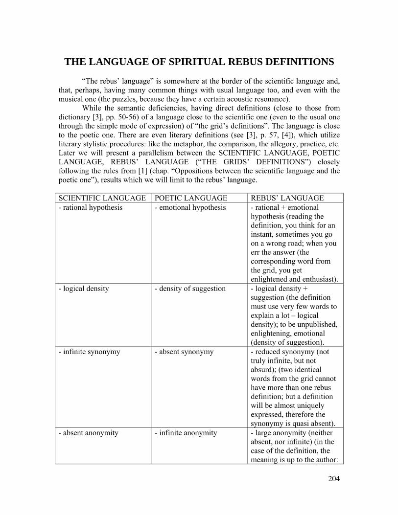
204
THE LANGUAGE OF SPIRITUAL REBUS DEFINITIONS “The rebus’ language” is somewhere at the border of the scientific language and, that, perhaps, having many common things with usual language too, and even with the musical one (the puzzles, because they have a certain acoustic resonance). While the semantic deficiencies, having direct definitions (close to those from dictionary [3], pp. 50-56) of a language close to the scientific one (even to the usual one through the simple mode of expression) of “the grid’s definitions”. The language is close to the poetic one. There are even literary definitions (see [3], p. 57, [4]), which utilize literary stylistic procedures: like the metaphor, the comparison, the allegory, practice, etc. Later we will present a parallelism between the SCIENTIFIC LANGUAGE, POETIC LANGUAGE, REBUS’ LANGUAGE (“THE GRIDS’ DEFINITIONS”) closely following the rules from [1] (chap. “Oppositions between the scientific language and the poetic one”), results which we will limit to the rebus’ language. SCIENTIFIC LANGUAGE POETIC LANGUAGE REBUS’ LANGUAGE - rational hypothesis - emotional hypothesis - rational + emotional
hypothesis (reading the definition, you think for an instant, sometimes you go on a wrong road; when you err the answer (the corresponding word from the grid, you get enlightened and enthusiast).
- logical density - density of suggestion - logical density + suggestion (the definition must use very few words to explain a lot – logical density); to be unpublished, enlightening, emotional (density of suggestion).
- infinite synonymy - absent synonymy - reduced synonymy (not truly infinite, but not absurd); (two identical words from the grid cannot have more than one rebus definition; but a definition will be almost uniquely expressed, therefore the synonymy is quasi absent).
- absent anonymity - infinite anonymity - large anonymity (neither absent, nor infinite) (in the case of the definition, the meaning is up to the author:
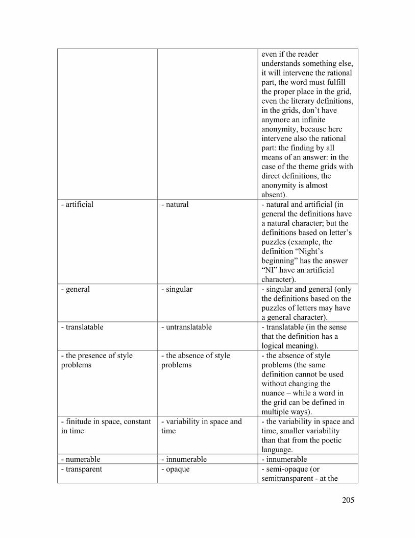
205
even if the reader understands something else, it will intervene the rational part, the word must fulfill the proper place in the grid, even the literary definitions, in the grids, don’t have anymore an infinite anonymity, because here intervene also the rational part: the finding by all means of an answer: in the case of the theme grids with direct definitions, the anonymity is almost absent).
- artificial - natural - natural and artificial (in general the definitions have a natural character; but the definitions based on letter’s puzzles (example, the definition “Night’s beginning” has the answer “NI” have an artificial character).
- general - singular - singular and general (only the definitions based on the puzzles of letters may have a general character).
- translatable - untranslatable - translatable (in the sense that the definition has a logical meaning).
- the presence of style problems
- the absence of style problems
- the absence of style problems (the same definition cannot be used without changing the nuance – while a word in the grid can be defined in multiple ways).
- finitude in space, constant in time
- variability in space and time
- the variability in space and time, smaller variability than that from the poetic language.
- numerable - innumerable - innumerable - transparent - opaque - semi-opaque (or
semitransparent - at the
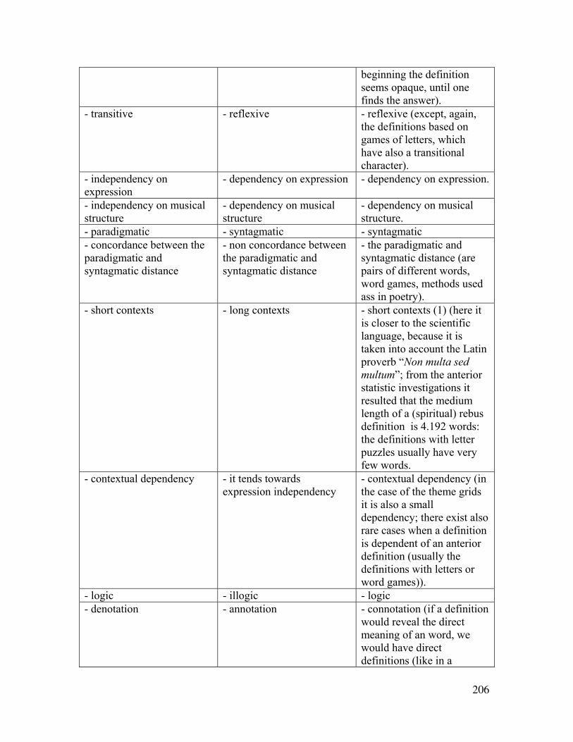
206
beginning the definition seems opaque, until one finds the answer).
- transitive - reflexive - reflexive (except, again, the definitions based on games of letters, which have also a transitional character).
- independency on expression
- dependency on expression - dependency on expression.
- independency on musical structure
- dependency on musical structure
- dependency on musical structure.
- paradigmatic - syntagmatic - syntagmatic - concordance between the paradigmatic and syntagmatic distance
- non concordance between the paradigmatic and syntagmatic distance
- the paradigmatic and syntagmatic distance (are pairs of different words, word games, methods used ass in poetry).
- short contexts - long contexts - short contexts (1) (here it is closer to the scientific language, because it is taken into account the Latin proverb “Non multa sed multum”; from the anterior statistic investigations it resulted that the medium length of a (spiritual) rebus definition is 4.192 words: the definitions with letter puzzles usually have very few words.
- contextual dependency - it tends towards expression independency
- contextual dependency (in the case of the theme grids it is also a small dependency; there exist also rare cases when a definition is dependent of an anterior definition (usually the definitions with letters or word games)).
- logic - illogic - logic - denotation - annotation - connotation (if a definition
would reveal the direct meaning of an word, we would have direct definitions (like in a

207
dictionary)) and then we would totally loose “the surprise”, “the spirituality”, “the ingenious”, “the spontaneity” of thematic grids, the definitions with denotative character.
- routine - creation - creation and … experience (not to call it routine!)
-general stereotypes - personal stereotypes - personal stereotypes (it exists even the so called grids of “personal manner” – (see [3], pp. 56-58)
- explicable - ineffable - ineffable … which explains it! (Taken separately, the definition, not-seen as a question, is ineffable taken along, with the answer becomes explicable: in general, the definition presents also an ambiguity degree (more tracks for guidance) – otherwise it would be banal – a degree of indetermination: it is used many times the proper sense instead of the figurative one, or reciprocally defined it has also its own logic, which becomes tangible once one finds the answer).
- lucidity - magic - magic – lucidity (in accordance with those that are immediately anterior) (at the beginning the rebus language dominates the person, until he finds the “key” when he’ll become at his turn the dominant – the poetic language.
- predictable - unpredictable - at the beginning is unpredictable, and becomes predictable after solving it: (unpredictable converted in predictable) .
208
CONSIDERATIONS REGARDING THE SCIENTIFIC LANGUAGE AND
“LITERARY LANGUAGE” As in nature nothing is absolute, evidently there will not exist a precise border between the scientific language and “the literary” one (the language used in literature): thus there will be zones where these two languages intersect. In [1], chapter “Instances between the scientific and poetic languages”, Solomon Marcus presents the differences between these two, differences that make them closer. We will skate a little on the edge of this material, presenting common parts of the scientific language and the literary language:
- both are geared to find the unpublished, the novelty - both suppose a creative process (finding the solution of a problem means
creation: writing of a phrase the same). - both literature and science have an art of being taught, studied and learned (the
methodology of teaching arithmetic, or Romanian language, etc.) . - in science too there is an esthetic (for example: “the mathematical esthetic”), the
same in literature there exists a logic (even the absurd of Eugene Ionesco, the myths of Mircea Eliade have their own specific logic: analogously, we can extend the idea to Tristan Tzara’s Dadaism, which has a specific logic (of construction; one cuts words from newspapers, mix them, and then form verses).
- the scientific development implies a literary development in a special sense: it appeared, thus, the science-fiction literature in literary writings which use informations obtained by science: contemporaneous literature treats also scientific problems (for example Augustin Buzura wrote the roman “The absents” describing the life of a medical researcher: the engineer poet George Stanca introduces technical terms in his poems; one verse from his volume “Maximum tenderness” sounds: “sin2 x + cos2 x = 1”!); analogously the engineer poet Gabriel Chifu (the volume “An interpretation of the Purgatory”) and mathematics professor Ovidiu Florentin, author of a volume even entitled “Formulas for the spirit” – each poem being considered as a momentous “formula” (depending of time, place, space, individual) for the spirit.
- even the writing of some contemporary novels inspired from the worker’s and peasant’s life requires a scientific documentation from the writers’ part.
The literature has an esthetic influence for science; there exist mathematical metaphors (see [1], [2]) and, in general, we can say “scientific metaphors”, one cannot know what ideas and relations will be discovered in science. The understanding degree (exegesis) of a poetry and of a literary text in general, depends also of the culture’s degree of each individual, of his initiation (the seniority in that domain), of his scientific knowledge.
- there are many scientists who, besides their scientific works, write also literary works or related domains (for example, the memories book of the academician (mathematician) Octav Onicescu “On the life’s roads”, the renown Romanian physician Gheorghe Marinescu writes poems (using Dacic words), under the penname George Dinizvor, the great Ion Barbu – Dan Barbilian excelled as a poet and as a mathematician. The great poet Vasile Voiculescu was a good physician; and the mathematics professor Aurel M. Buricea writes poetry, analogously the mathematician Ovidiu Florentin –
209
Florentin Smarandache writes poems and mathematics articles; in the world literature we find the poet-mathematician Omar Khayyam and Lewis Caroll – Charles L. Dodgson), but writers that would do fundamental scientific or technical research don’t quite exist!
REFERENCES
[1] Marcus, Solomon – “Poetica matematică”, Ed. Academiei, Bucharest, 1970.
[2] Marcus, Solomon – “Introducere în lingvistica matematică”, Bucharest, 1966.
[3] Andrei, Dr. N. – “Îndreptar rebusist”, Ed. Sport-Turism, Bucharest, 1981. [4] Magazine collection “Rebus”, 1979-1982. [5] Marcus, Solomon – “Limbajul poetic - limbajul matematic”, in the
“Orizont” magazine (Timişoara), 26 March 1982.
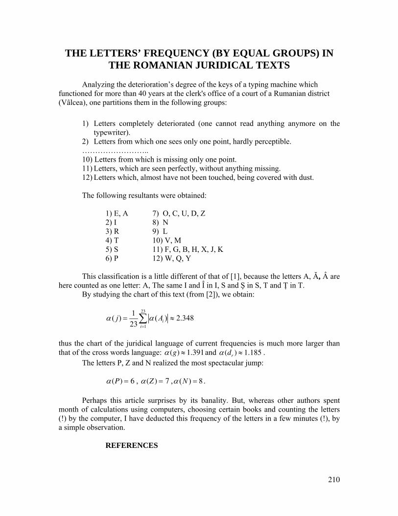
210
THE LETTERS’ FREQUENCY (BY EQUAL GROUPS) IN THE ROMANIAN JURIDICAL TEXTS
Analyzing the deterioration’s degree of the keys of a typing machine which functioned for more than 40 years at the clerk's office of a court of a Rumanian district (Vâlcea), one partitions them in the following groups:
1) Letters completely deteriorated (one cannot read anything anymore on the
typewriter). 2) Letters from which one sees only one point, hardly perceptible. …………………….. 10) Letters from which is missing only one point. 11) Letters, which are seen perfectly, without anything missing. 12) Letters which, almost have not been touched, being covered with dust. The following resultants were obtained:
1) E, A 7) O, C, U, D, Z 2) I 8) N 3) R 9) L 4) T 10) V, M 5) S 11) F, G, B, H, X, J, K 6) P 12) W, Q, Y
This classification is a little different of that of [1], because the letters A, Ă, Â are here counted as one letter: A, The same I and Î in I, S and Ş in S, T and Ţ in T.
By studying the chart of this text (from [2]), we obtain:
23
1
1( ) ( ) 2.34823 i
ij Aα α
=
= ≈∑
thus the chart of the juridical language of current frequencies is much more larger than that of the cross words language: α(g) ≈ 1.391and α (dr ) ≈ 1.185 . The letters P, Z and N realized the most spectacular jump: α(P) = 6 , α(Z ) = 7 , ( ) 8Nα = . Perhaps this article surprises by its banality. But, whereas other authors spent month of calculations using computers, choosing certain books and counting the letters (!) by the computer, I have deducted this frequency of the letters in a few minutes (!), by a simple observation. REFERENCES
211
[1] Marcus, Solomon – “Poetica matematică”, Editura Academiei, Bucharest, 1970 (translated in German, Athenäum, Frankfurt, 1973).
[2] Smarandache, Florentin – “A mathematical linguistic approach to Rebus”, Tome XXVIII, 1983, collection “Cahiers de linguistique théorique et appliquée”, Tome XX, 1983, No. 1, pp. 67-76, Bucharest.
212
MATHEMATICAL FANCIES AND PARADOXES
MISCELLANEA
1. Archimedes’ “fixed point theorem”: Give me a fixed point in space, and I shall lift the Earth”.
2. MATHEMATICAL LINGUISTICS1
Poem by Ovidiu Florentin2
Definition A word’s sequence converges if it is found in a neighborhood of our heart.
* The hermetic verses are linear equations.
* Theorem For any X there is no Y such that Y knows everything which X knows. And the reciprocal. The proof is very intricate and long, and we will present it. We leave it to the readers to solve it!
** Smarandache’s law: Give me a point in space and I shall write the proposition
behind it. Final Motto - O, MATHEMATICS, YOU, EXPRESSION OF THE ESSENTIAL IN
NATURE! 1 Volume which includes this mathematical poem (pp. 39-41). 2 (Translated from Romanian by the author.) It is the mathematician’s pen
name. He wrote many poetical volumes (in Romanian and French), as “Legi de compoziţie internă. Poeme cu…probleme!” (Laws of internal composition. Poems with…problems!), Ed. El Kitab, Fès, Morocco, 1982.
213
AMUSING PROBLEMS
1. Calculate the volume of a square.
(Solution: Volume = Area of the Base x Height = Side2 x 0 = 0! We look at the square as an extreme case of parallelepiped with the height null.)
2. ? x 7 = 2?
(Solution: of course 2
7× 7 = 2 !)
3. Ten birds are on a fence. A hunter shoots three of them. How many birds remain? (Answer: none, because the three dead birds fell down from the fence and the other seven flew away!)
4. Ten birds are in a meadow. A hunter shoots three of them. How many birds remain?
(Answer: three birds, the dead birds, because the others flew away!) 5. Ten birds are in a cage. A hunter shoots three of them. How many
birds remain? (Answer: ten birds, dead and alive, because none could get out!) 6. Ten birds are up in the sky. A hunter shoots three of them. How many
birds remain? (Answer: seven birds, at last, those who are still flying and those that fell down!) 7. Prove that the equation 2X X= + has two distinct solutions. (Answer: X = ±∞ !) 8. (Solving Fermat’s last theorem) Prove that for any non-null integer n,
the equation Xn + Y n = Z n , XYZ ≠ , has at least one integer solution! (Answer: (a) n ≥ 1. Let Xk = Yk = Zk = 2k , 1, 2,3,...k = All Xk ∈N , K ≥ 1 .
lim k NkL X ∈→∞
= . But L = ∞ ∈N , that is the integer infinite, and ∞n + ∞n = ∞n ! If n is
even, the equation has eight distinct integer solutions: X = Y = Z = ±∞ ! Similarly, we take the negative infinite integer: - ∞0Z]
(b) n ≤ −1 . Clearly there are at last eight distinct integer solutions: X = Y = Z = ±∞ !)
WHERE IS THE ERROR IN THE BELOW DIOPHANTINE EQUATIONS ?
Statement: (1) To solve in Z the equation: 14 26 20x y+ = − . “Resolution”: The integer general solution is:
x = −26k + 6
y = 14k − 4
⎧⎨⎩
(k ∈Z)
(2) To solve in Z the equation: 15 37 12 0x y z− + = . “Resolution” The integer general solution is:
214
41545 5
x ky kz k
= +⎧⎪ =⎨⎪ = −⎩
(k ∈Z)
(3) To solve in Z the equation: 3x − 6y + 5z − 10w = 0 . “Resolution” the equation is written: 3(x − 2y) + 5z − 10w = 0 . Since , , , x y z w are integer variables, it results that 3 divides z and that 3 divides
w . I. e: z = 3t1 (t1 ∈Z) and w = 3t2 (t2 ∈Z) . Thus 3(x − 2y) + 3(5t1 − 10t2 ) = 0 where x − 2y + 5t1 − 10t2 = 0 .
Then:
x = 2k1 + 5k2 − 10k3
y = k1
z = 3k2
w = 3k3
⎧
⎨
⎪⎪
⎩
⎪⎪
with (k1,k2 , k3 ∈Z3) ,
constitute the integer general solution of the equation. Find the error of each “resolution”. SOLUTIONS. (1) x = −26k + 6 and y = 14k − 4 ( k ∈Z ) is an integer solution for the equation
(because it verifies it), but it is not the general solution, because x = −7 and y = 3 verify the equation, they are a particular integer solution, but:
−26k + 6 = −7
14k − 4 = 3
⎧⎨⎩
implies that k =1
2 (does not belong to Z ).
Thus one cannot obtain this particular from the previous general solution.
The true general solution is: x = −13k + 6
y = 7k − 4
⎧⎨⎩
(k ∈Z) . (from [1])
(2) In the same way, x = 5 , y = 3 , z = 3 is a particular solution of the equation, but which cannot be obtained from the “general solution” because:
4 5 1115 3 5845 5 345
k k
k k
k k
⎧⎪ + = ⇒ = −⎪⎪ = ⇒ =⎨⎪⎪ − = ⇒ =⎪⎩
,
contradictions.
The integer general solution is: x = k1
y = 3k1 + 12k2
z = 8k1 + 37k2
⎧
⎨⎪
⎩⎪
(with (k1,k2 ) ∈Z2 , cf. [1]).
(3) The error is that: “3 divides ( 5z − 10w )” does not imply that “3 divides z and 3 divides w ”. If one believes that one loses solutions, then this is true because
215
(x, y, z,w) = (−5,0,5,1) constitutes a particular integer solution, which cannot be obtained from the “solution” of the statement.
The correct resolution is: 3(x − 2y) + 5(z − 2w) = 0 , that is 3p1 + 5 p2 = 0 , with p1 = x − 2y in Z , and p2 = z − 2w in Z .
It results that: 1
2
5 2in
3 2p k x yp k z w
= − = −⎧⎨ = = −⎩
Z .
From which one obtains the integer general solution: 1 2
1
2 3
3
2 5
3 2
x k ky k
z k k
w k
= −⎧⎪ =⎪⎨ = +⎪⎪ =⎩
with (k1,k2 ,k3) ∈Z3
[1] One can find these solutions using: Florentin SMARANDACHE - “Un
algorithme de résolution dans l’ensemble des numbers entiers pour les équations linéaires”.
WHERE IS THE ERROR ON THE BELOW INTEGRALS ?
Let the function f :R → R be defined by ( ) 2sin cosf x x x= . Let us calculate its primitive: (1) First method.
22 22sin cos 2 2 sin
2ux x dx u du u x= = = =∫ ∫ , with u = sin x .
One thus has F1(x) = sin2 x . (2) Second method:
22sin cos 2 cos ( sin ) 2 x x dx x x dx v dv v= − − = − = −∫ ∫ ∫ ,
thus F2 (x) = − cos2 x (3) Third method:
1 1 12sin cos sin 2 (sin2 ) 2 sin cos2 2 2
x x dx x dx x dx t dt t= = = = −∫ ∫ ∫ ∫
thus F3(x) = −1
2cos2x .
One thus obtained 3 different primitives of the same function. How is this possible? Answer: There is no error! It is known that a function admits an infinity of
primitives (if it admits one), which differ only by one constant. In our example we have:
F2 (x) = F1(x) − 1 for any real x , and F3(x) = F1(x) −1
2 for any real x .
216
WHERE IS THE ERROR IN THE BELOW REASONING BY
RECURRENCE ?
At an admission contest at an University, was given the following problem: “Find the polynomials P(x) with real coefficients such that xP(x − 1) = (x − 3)P(x) , for all x real.” Some candidates believed that they would be able to show by recurrence that the polynomials of the statement are those which verify the following property: P(x) = 0 for all natural values. In fact, they said, if one puts x = 0 in this relation, it results that 0 ⋅ P(−1) = −3 ⋅ P(0) , therefore P(0) = 0 . Likewise, with x = 1 , one has: 1 ⋅ P(0) = −2 ⋅ P(1) , therefore P(1) = 0 , etc. Let’s suppose that the property is true for ( n − 1 ), therefore P(n − 1) = 0 , and we are looking to prove it for n : One has: n ⋅ P(n − 1) = (n − 3) ⋅ P(n) , and since P(n − 1) = 0 , it results that P(n) = 0 . Where the proof failed? Answer: If the candidates would have checked for the rank n = 3 , they would have found that: 3 ⋅ P(2) = 0 ⋅ P(3) thus 0 = 0 ⋅ P(3) , which does not imply that P(3) , is null: in fact this equality is true for any real P(3) . The error, therefore, is created by the fact that the implication: “ (n − 3) ⋅ P(n) = n ⋅ P(n − 1) = 0 ⇒ P(n) = 0 ” is not true. One can find easily that P(x) = x(x − 1)(x − 2)k , k ∈R .
WHERE IS THE ERROR? Given the functions f , g :R → R , defined as follows:
, 3( )
, 3
x
x
e xf x
e x−
⎧ ≤⎪= ⎨>⎪⎩
and 2 , 0
( )2 7, 3x x
g xx x
⎧ ≤= ⎨
− + >⎩
Compute f g . “Solution”: We can write:
, 0( ) , 0 3
, 0
x
x
x
e xf x e x
e x−
⎧ ≤⎪
= < ≤⎨⎪ >⎩
and
2 , 0( ) 2 7, 0 3
2 7, 3
x xg x x x
x x
⎧ ≤⎪= − + < ≤⎨⎪− + >⎩
from where 2
2 7
2 7
, 0( )( ) ( ( )) , 0 3
, 3
x
x
x
e xf g x f g x e x
e x
− +
−
⎧ ≤⎪⎪= = < ≤⎨⎪ >⎪⎩
217
and :f g →R R . Correct solution:
( )
( )
, if ( ) 3( ( ))
, if ( ) 3
g x
g x
e g xf g f g x
e g x−
⎧ ≤⎪= = ⎨>⎪⎩
:f g →R R
2 3 [ 3,0]( ) 3
2 7 3 [2, )
x xg x or
x x
⎧ ≤ ⇒ ∈ −⎪
≤ ⇒ ⎨⎪− + ≤ ⇒ ∈ +∞⎩
2 3 ( , 3)( ) 3
2 7 3 (0,2)
x xg x or
x x
⎧ > ⇒ ∈ −∞ −⎪
> ⇒ ⎨⎪− + > ⇒ ∈⎩
Therefore
2
2
2 7
2 7
, ( , 3)
, [ 3,0))( ), (0, 2), [2, )
x
x
x
x
e x
e xf g xe xe x
−
−
−
⎧ ∈ −∞ −⎪⎪ ∈ −= ⎨
∈⎪⎪ ∈ +∞⎩
[Published in “Gazeta matematică”, nr.7/1981, Anul LXXXVI, pp. 282-283.]
WHERE IS THE ERROR IN THE BELOW SYSTEM OF INEQUALITIES ?
Solve the following inequalities system:
0 (1)0 (2)2 3 0 (3)
3 4 4 (4)
xyx y z
x y z
≥⎧⎪ ≥⎪⎨ − + ≥⎪⎪− − + ≥⎩
“Solution”: Multiply the third inequality by 3 and add it to the fourth inequality. The sense will be conserved. It results:
−7y + 13z ≥ 4 , or z ≥1
13(7y + 4) .
Therefore, x ≥ 0 and y ≥ 0 (from the inequalities (1) and (2))
and z ≥1
13(7y + 4) (*).
218
But x = 13 ≥ 0 , y = 0 ≥ 0 , and z = 2 ≥4
13=
1
13(7 ⋅ 0 + 4) verifies (*). But we
observe that it does not verify the inequalities system, because substituting in the fourth inequality we obtain: −3 ⋅13 − 0 + 4 ⋅ 2 ≥ 4 which is not true.
Where is the contradiction? Solution. The previous solution is incomplete. We didn’t intersect all four inequalities.
Giving a geometrical interpretation in R3 , and writing the inequalities as equations, we have, in fact, four planes, each dividing the space in semi spaces. Therefore, the system’s solution will be formed by the points which belong to the intersection of those four semi spaces, (each inequality determines a semi space). The inequality obtained by adding the third inequality with the fourth represents, is, in fact, another semi space that includes the system’s solution, and it does not simplify the system (in the sense that we cannot eliminate any of the system’s inequalities).
Therefore x = 0 , y = 3 , z =5
13 verifies (*) but it does not verify, this time, the
third inequality (although the fourth one is verified).
THE ILLOGICAL MATHEMATICS! Find a “logic” for the following statements: (1) 4 − 5 ≈ 5!
(2) 8 divided by two is equal to zero! (3) 10 minus 1 equals 0. (4) f (x)∫ dx = f (x) !
(5) 8+8=8! Solutions:
These mathematical fantasies are entertainments, amusing problems; they disregard current logic, but having their own “logic”, fantasist logic: thus
(1) can be explained if one does not consider “4 - 5” as the writing of “4 minus 5” but that of “from 4 to 5”; from which a reading of the statement “ 4 − 5 ≈ 5 ” should be: “between 4 and 5, but closer to 5”.
(2) 8 can be divided by two … in the following way:…, i. e. it will be cut into two equal parts, which are equal to “0” above and below the cutting line!
(3) “10 minus 1” can be treated as: the two typographical characters 1, 0 minus the 1, which justifies that there remains the character 0.
(4) The sign will be considered as the opposite function of the integral. (5) The operation “ ∞ + ∞ = ∞ ” is true: writing it vertically:
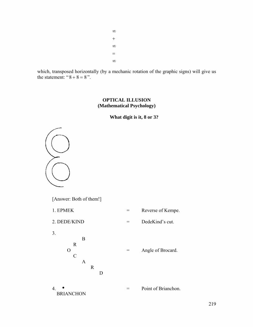
219
∞+∞=∞
which, transposed horizontally (by a mechanic rotation of the graphic signs) will give us the statement: “ 8 + 8 = 8 ”.
OPTICAL ILLUSION (Mathematical Psychology)
What digit is it, 8 or 3?
[Answer: Both of them!] 1. EPMEK = Reverse of Kempe. 2. DEDE/KIND = DedeKind’s cut. 3.
B R O = Angle of Brocard. C A R D
4.
BRIANCHON• = Point of Brianchon.
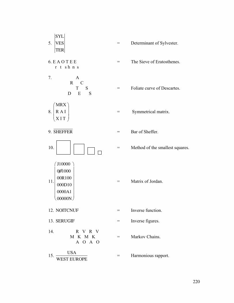
220
5. SYL
VES
TER
= Determinant of Sylvester.
6. E A O T E E = The Sieve of Eratosthenes. r t s h n s
7. A R C T S = Foliate curve of Descartes. D E S
8. MRXR A IX I T
⎛ ⎞⎜ ⎟⎜ ⎟⎜ ⎟⎝ ⎠
= Symmetrical matrix.
9. SHEFFER = Bar of Sheffer. 10. = Method of the smallest squares.
11.
J10000
001000
00R100
000D10
0000A1
00000N
⎛
⎝
⎜⎜⎜⎜⎜⎜⎜
⎞
⎠
⎟⎟⎟⎟⎟⎟⎟
= Matrix of Jordan.
12. NOITCNUF = Inverse function. 13. SERUGIF = Inverse figures. 14. R V R V
M K M K = Markov Chains. A O A O
15. USA
WEST EUROPE = Harmonious rapport.
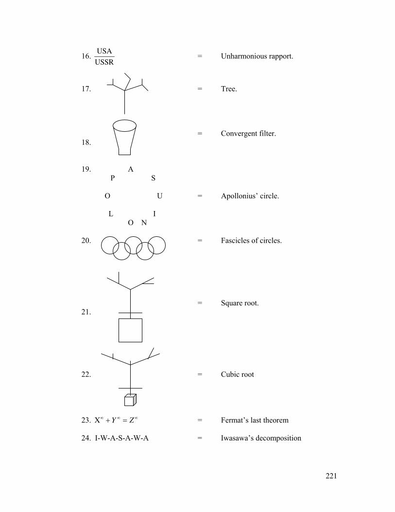
221
16. USA
USSR = Unharmonious rapport.
17. = Tree. = Convergent filter.
18.
19. A
P S O U = Apollonius’ circle. L I
O N 20. = Fascicles of circles.
= Square root. 21.
22. = Cubic root 23. X∞ + Y ∞ = Z ∞ = Fermat’s last theorem 24. I-W-A-S-A-W-A = Iwasawa’s decomposition
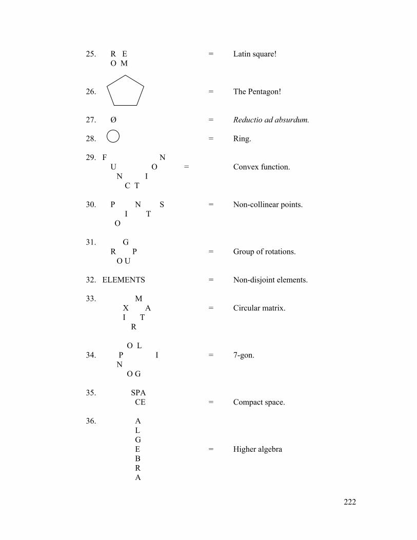
222
25. R E = Latin square! O M
26. = The Pentagon!
27. Ø = Reductio ad absurdum. 28. = Ring. 29. F N U O = Convex function. N I C T
30. P N S = Non-collinear points. I T
O
31. G R P = Group of rotations.
O U 32. ELEMENTS = Non-disjoint elements.
33. M X A = Circular matrix. I T R O L 34. P I = 7-gon. N O G 35. SPA
CE = Compact space.
36. A L G E = Higher algebra B R A

223
37. = Vicious circle 38. A
R I T = The higher arithmetic. H M E T I C
39. = Square angle.
40. SYMBOL OF (LEOPOLD)
KRONECKER = L.K.
41. KOLMOGOROV’S SPACE = USSR.
42. LANGUAGE OF CHOMSKY = American.
43. GRAMMAR OF KLEENE = English. 44. CATASTROPHIC POINT = Atom bomb. 45. MACHINE OF TURING = Motor car. 46. NUMBER OF GOLD = 79 (Chemically). 47. FLY OF LA HIRE = Insect. 48. MOMENT OF INERTIA = Apathy. 49. AXIOM OF SEPARATION = Divorce. 50. CLOSED SET = Prisoners. 51. RUSSIAN MULTIPLICATION = Conquest.
52. SLIPS OF MÖBUS = Bathing trunks.
A
224
53. SINGULAR CARDINAL = Mazarin (1602-1661, France). 54. CLAN OF LEBESGUE = His family. 55. SPHERE OF RIEMANN = Head. 56. MATHEMATICAL HOPE = Fields prize. 57. CRITICAL WAY = Slope. 58. BOTTLE OF KLEIN = Beer bottle. 59. CONSTANT OF EULER = Mathematics. 60. CONTRACTING FUNCTION = Frost.
61. BILINEAR COMBINATION = Concubine. 62. HARDY SPACE = England. 63. INTRODUCTION TO ALGEBRA! = AL. 64. INTRODUCTORY ECONOMETRICS = ECO. 65. BOREL BODY = Corpse. 66. CHOICE FUNCTION = Marriage. 67. GEOMETRICAL PLACES = ATHENA, ERLANGEN, etc. [Published in GAMMA, Year IX, Nr. 1, November 1986.]
MATHEMATICAL LOGIC How many propositions are true and which ones from the following:
1. There exists one false proposition amongst those n propositions. 2. There exist two false propositions amongst those n propositions. ……………………………………………………………………. … There exist i false propositions amongst those n propositions. ……………………………………………………………………. n. There exist n false propositions amongst those n propositions.
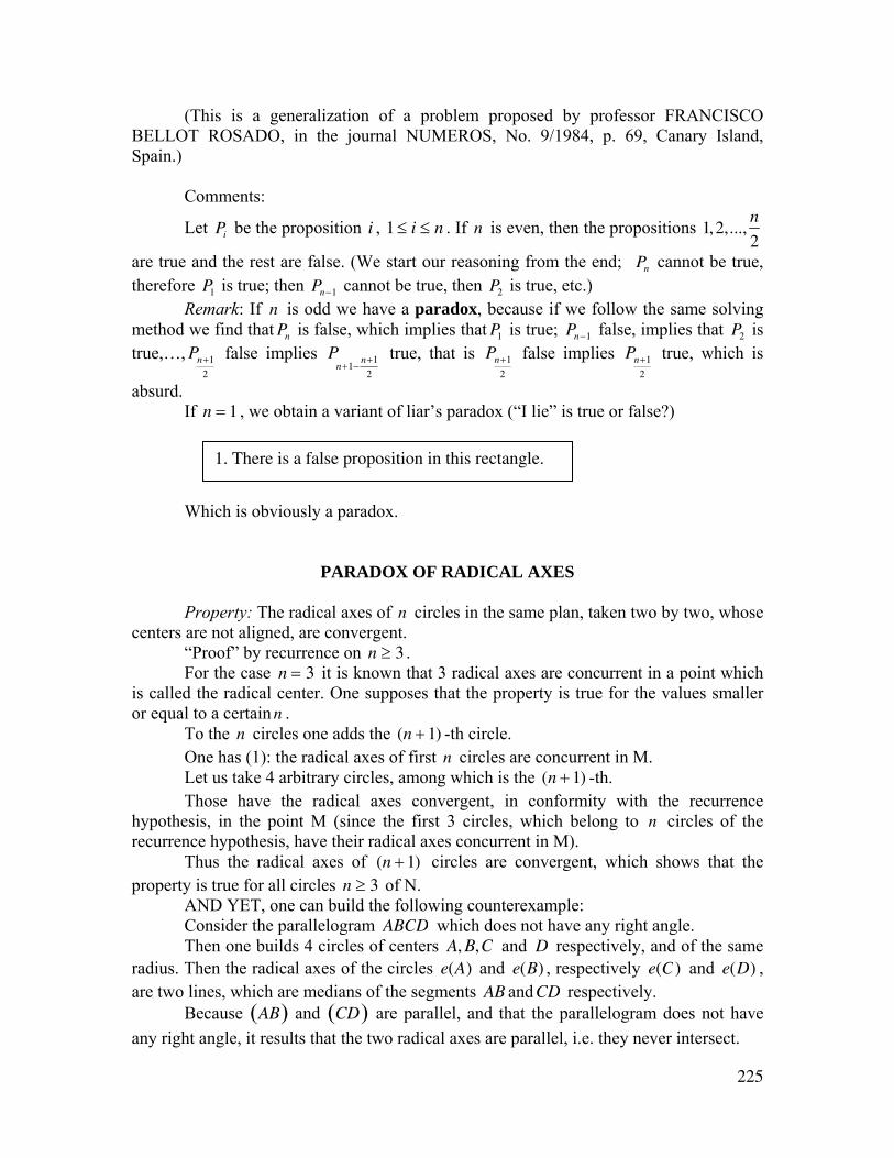
225
(This is a generalization of a problem proposed by professor FRANCISCO BELLOT ROSADO, in the journal NUMEROS, No. 9/1984, p. 69, Canary Island, Spain.)
Comments:
Let Pi be the proposition i , 1 ≤ i ≤ n . If n is even, then the propositions 1,2,...,n
2
are true and the rest are false. (We start our reasoning from the end; Pn cannot be true, therefore P1 is true; then Pn−1 cannot be true, then P2 is true, etc.)
Remark: If n is odd we have a paradox, because if we follow the same solving method we find that Pn is false, which implies that P1 is true; Pn−1 false, implies that P2 is true,…, Pn+1
2
false implies Pn+1−
n+1
2
true, that is Pn+1
2
false implies Pn+1
2
true, which is
absurd. If n = 1 , we obtain a variant of liar’s paradox (“I lie” is true or false?)
Which is obviously a paradox.
PARADOX OF RADICAL AXES
Property: The radical axes of n circles in the same plan, taken two by two, whose centers are not aligned, are convergent. “Proof” by recurrence on n ≥ 3 . For the case n = 3 it is known that 3 radical axes are concurrent in a point which is called the radical center. One supposes that the property is true for the values smaller or equal to a certain n . To the n circles one adds the (n + 1) -th circle. One has (1): the radical axes of first n circles are concurrent in M. Let us take 4 arbitrary circles, among which is the (n + 1) -th. Those have the radical axes convergent, in conformity with the recurrence hypothesis, in the point M (since the first 3 circles, which belong to n circles of the recurrence hypothesis, have their radical axes concurrent in M). Thus the radical axes of (n + 1) circles are convergent, which shows that the property is true for all circles n ≥ 3 of N. AND YET, one can build the following counterexample: Consider the parallelogram ABCD which does not have any right angle. Then one builds 4 circles of centers A, B,C and D respectively, and of the same radius. Then the radical axes of the circles e(A) and e(B) , respectively e(C) and e(D) , are two lines, which are medians of the segments AB andCD respectively. Because AB( ) and CD( ) are parallel, and that the parallelogram does not have any right angle, it results that the two radical axes are parallel, i.e. they never intersect.
1. There is a false proposition in this rectangle.
226
Can we explain this (apparent!) contradiction with the previous property? Response: The “property “is true only for n = 3 . However in the demonstration suggested one utilizes the premise (distorted) according to which for m + 4 the property would be true. To complete the proof by recurrence it would have been necessary to be able to prove that P(3) ⇒ P(4) , which is not possible since P(3) is true but the counterexample proves that P(4) is false.
A CLASS OF PARADOXES Let A be an attribute and non-A its negation. P1. ALL IS ”A”, THE “NON-A” TOO. Examples:
E11 : All is possible, the impossible too. E12 : All are present, the absentee too. E13 : All is finite, the infinite too. P2. ALL IS “NON-A”, THE “A” TOO. Examples:
E21 : All is impossible, the possible too. E22 : All are absent, the present too.
E23 : All is infinite, the finite too. P3. NOTHING IS “A” NOT EVEN THE “A”. Examples:
E31 : Nothing is perfect, not even the perfect. E32 : Nothing is absolute, not even the absolute.
E33 : Nothing is finite, not even the finite.
Remark: P1 ⇔ P2 ⇔ P3 . More generally: ALL (verb) “A”, the “NON-A” too. Of course, from these appear unsuccessful paradoxes, but the proposed method obtains beautiful ones. Look at a pun, which reminds you of Einstein: All is relative, the (theory of) relativity too! So: The shortest way between two pints is the meandering way! The unexplainable is, however, explained by this word: “unexplainable”! [Presented at “The Eugene Strens Memorial on Intuitive and Recreational Mathematics and its History”, University of Calgary, Alberta, Canada; July 27 – August 2, 1986.
227
Partially published in “Beta”, Craiova, 1987; “Gamma”, Braşov, 1987; and “Abracadabra”, Salinas (California), USA, 1993-4.]
Articles, notes,
generalizations, paradoxes,
miscellaneous in
Mathematics, Linguistics,
and Education.
7815999 730486
ISBN 1-59973-048-0
53995>