vol3 guidelines
TRANSCRIPT

8/8/2019 Vol3 Guidelines
http://slidepdf.com/reader/full/vol3-guidelines 1/146
Traffic Analysis Toolbox Volume III:
Guidelines for Applying Traffic
Microsimulation Modeling Software
PUBLICATION NO. FHWA-HRT-04-040 JULY 2004
Research, Development, and Technology
Turner-Fairbank Highway Research Center
6300 Georgetown Pike
McLean, VA 22101-2296
8/8/2019 Vol3 Guidelines
http://slidepdf.com/reader/full/vol3-guidelines 2/146
8/8/2019 Vol3 Guidelines
http://slidepdf.com/reader/full/vol3-guidelines 3/146
Technical Report Documentation Page
1. Report No. FHWA-HRT-04-040
2. Government Accession No. 3. Recipient’s Catalog No.
5. Report Date
June 2004
4. Title and Subtitle
Traffic Analysis Toolbox
Volume III: Guidelines for Applying Traffic MicrosimulationSoftware
6. Performing Organization Code
7. Author(s)
Richard Dowling, Alexander Skabardonis, Vassili Alexiadis
8. Performing Organization Report No.
10. Work Unit No.9. Performing Organization Name and Address
Dowling Associates, Inc.
180 Grand Avenue, Suite 250
Oakland, CA 94612
11. Contract or Grant No.
DTFH61-01-C-00181
13. Type of Report and Period Covered
Final Report, May 2002 – August 2003
12. Sponsoring Agency Name and Address
Office of Operations
Federal Highway Administration
400 7th Street, S.W.
Washington, D.C. 20590
14. Sponsoring Agency Code
15. Supplementary Notes
FHWA COTR: John Halkias, Office of Transportation Management
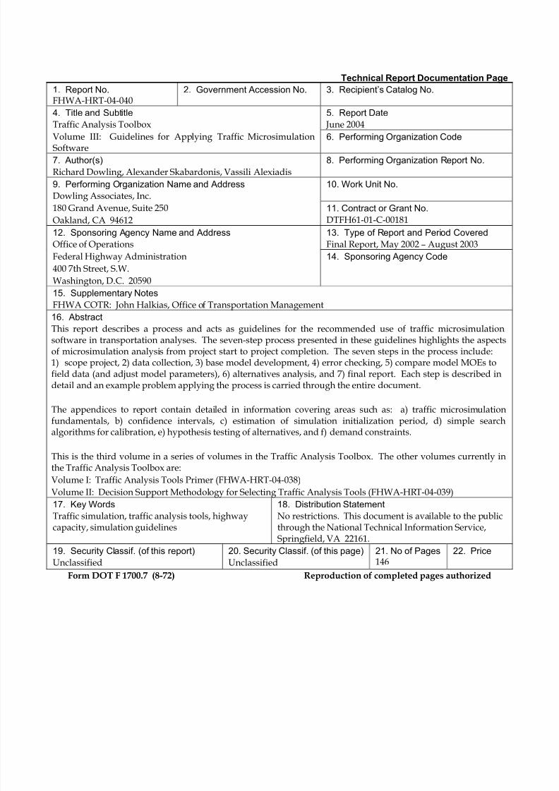
16. Abstract
This report describes a process and acts as guidelines for the recommended use of traffic microsimulationsoftware in transportation analyses. The seven-step process presented in these guidelines highlights the aspectsof microsimulation analysis from project start to project completion. The seven steps in the process include:1) scope project, 2) data collection, 3) base model development, 4) error checking, 5) compare model MOEs tofield data (and adjust model parameters), 6) alternatives analysis, and 7) final report. Each step is described indetail and an example problem applying the process is carried through the entire document.
The appendices to report contain detailed in information covering areas such as: a) traffic microsimulationfundamentals, b) confidence intervals, c) estimation of simulation initialization period, d) simple searchalgorithms for calibration, e) hypothesis testing of alternatives, and f) demand constraints.
This is the third volume in a series of volumes in the Traffic Analysis Toolbox. The other volumes currently inthe Traffic Analysis Toolbox are:
Volume I: Traffic Analysis Tools Primer (FHWA-HRT-04-038)
Volume II: Decision Support Methodology for Selecting Traffic Analysis Tools (FHWA-HRT-04-039)
17. Key Words
Traffic simulation, traffic analysis tools, highwaycapacity, simulation guidelines
18. Distribution Statement
No restrictions. This document is available to the publicthrough the National Technical Information Service,Springfield, VA 22161.
19. Security Classif. (of this report)Unclassified 20. Security Classif. (of this page)Unclassified 21. No of Pages 146 22. Price
Form DOT F 1700.7 (8-72) Reproduction of completed pages authorized
8/8/2019 Vol3 Guidelines
http://slidepdf.com/reader/full/vol3-guidelines 4/146
ii
SI* (MODERN METRIC) CONVERSION FACTORSAPPROXIMATE CONVERSIONS TO SI UNITS
Symbol When You Know Multiply By To Find Symbol
LENGTHin inches 25.4 millimeters mm
ft feet 0.305 meters m
yd yards 0.914 meters mmi miles 1.61 kilometers km
AREAin
2square inches 645.2 square millimeters mm
2
ft2
square feet 0.093 square meters m2
yd2
square yard 0.836 square meters m2
ac acres 0.405 hectares ha
mi2
square miles 2.59 square kilometers km2
VOLUMEfl oz fluid ounces 29.57 milliliters mL
gal gallons 3.785 liters Lft
3cubic feet 0.028 cubic meters m
3
yd3
cubic yards 0.765 cubic meters m3
NOTE: volumes greater than 1000 L shall be shown in m3
MASSoz ounces 28.35 grams g
lb pounds 0.454 kilograms kgT short tons (2000 lb) 0.907 megagrams (or "metric ton") Mg (or "t")
TEMPERATURE (exact degrees)oF Fahrenheit 5 (F-32)/9 Celsius
oC
or (F-32)/1.8
ILLUMINATIONfc foot-candles 10.76 lux lxfl foot-Lamberts 3.426 candela/m
2cd/m
2
FORCE and PRESSURE or STRESSlbf poundforce 4.45 newtons N
lbf/in2
poundforce per square inch 6.89 kilopascals kPa
APPROXIMATE CONVERSIONS FROM SI UNITS
Symbol When You Know Multiply By To Find Symbol
LENGTHmm millimeters 0.039 inches in
m meters 3.28 feet ftm meters 1.09 yards yd
km kilometers 0.621 miles mi
AREAmm
2square millimeters 0.0016 square inches in
2
m2
square meters 10.764 square feet ft2
m2
square meters 1.195 square yards yd2
ha hectares 2.47 acres ac
km2
square kilometers 0.386 square miles mi2
VOLUMEmL milliliters 0.034 fluid ounces fl oz
L liters 0.264 gallons gal
m3
cubic meters 35.314 cubic feet ft3
m3
cubic meters 1.307 cubic yards yd3
MASSg grams 0.035 ounces oz
kg kilograms 2.202 pounds lbMg (or "t") megagrams (or "metric ton") 1.103 short tons (2000 lb) T
TEMPERATURE (exact degrees) oC Celsius 1.8C+32 Fahrenheit
oF
ILLUMINATIONlx lux 0.0929 foot-candles fc
cd/m2
candela/m2
0.2919 foot-Lamberts fl
FORCE and PRESSURE or STRESSN newtons 0.225 poundforce lbf
kPa kilopascals 0.145 poundforce per square inch lbf/in2
*SI is the symbol for th International System of Units. Appropriate rounding should be made to comply with Section 4 of ASTM E380.e
(Revised March 2003)
8/8/2019 Vol3 Guidelines
http://slidepdf.com/reader/full/vol3-guidelines 5/146
iii
Table of Contents
Introduction ............................................................................................................................ 1
1.0 Microsimulation Study Organization/Scope ........................................................... 111.1 Study Objectives................................................................................................... 111.2 Study Breadth ....................................................................................................... 111.3 Analytical Approach Selection ........................................................................... 141.4 Analytical Tool Selection (Software) ................................................................. 15
1.4.1 Technical Capabilities .............................................................................. 151.4.2 Input/Output/Interfaces......................................................................... 161.4.3 User Training/Support............................................................................ 161.4.4 Ongoing Software Enhancements .......................................................... 16
1.5 Resource Requirements....................................................................................... 161.6 Management of a Microsimulation Study ........................................................ 181.7 Example Problem: Study Scope and Purpose .................................................. 19
2.0 Data Collection/Preparation........................................................................................ 232.1 Required Data....................................................................................................... 23
2.1.1 Geometric Data.......................................................................................... 242.1.2 Control Data .............................................................................................. 242.1.3 Demand Data............................................................................................. 24
2.2 Calibration Data ................................................................................................... 272.2.1 Field Inspection......................................................................................... 282.2.2 Travel Time Data....................................................................................... 282.2.3 Point Speed Data....................................................................................... 29
2.2.4 Capacity and Saturation Flow Data ....................................................... 292.2.5 Delay and Queue Data............................................................................. 30
2.3 Data Preparation/Quality Assurance ............................................................... 302.4 Reconciliation of Traffic Counts ......................................................................... 312.5 Example Problem: Data Collection and Preparation ...................................... 32
3.0 Base Model Development............................................................................................ 353.1 Link-Node Diagram: Model Blueprint.............................................................. 353.2 Link Geometry Data............................................................................................. 383.3 Traffic Control Data at Intersections and Junctions ........................................ 393.4 Traffic Operations and Management Data for Links ...................................... 39
3.5 Traffic Demand Data ........................................................................................... 393.6 Driver Behavior Data ........................................................................................... 403.7 Events/Scenarios Data ........................................................................................ 403.8 Simulation Run Control Data............................................................................. 403.9 Coding Techniques for Complex Situations..................................................... 413.10 Quality Assurance/Quality Control (QA/QC) Plan ...................................... 423.11 Example Problem: Base Model Development.................................................. 42
8/8/2019 Vol3 Guidelines
http://slidepdf.com/reader/full/vol3-guidelines 6/146
iv
Table of Contents (continued)
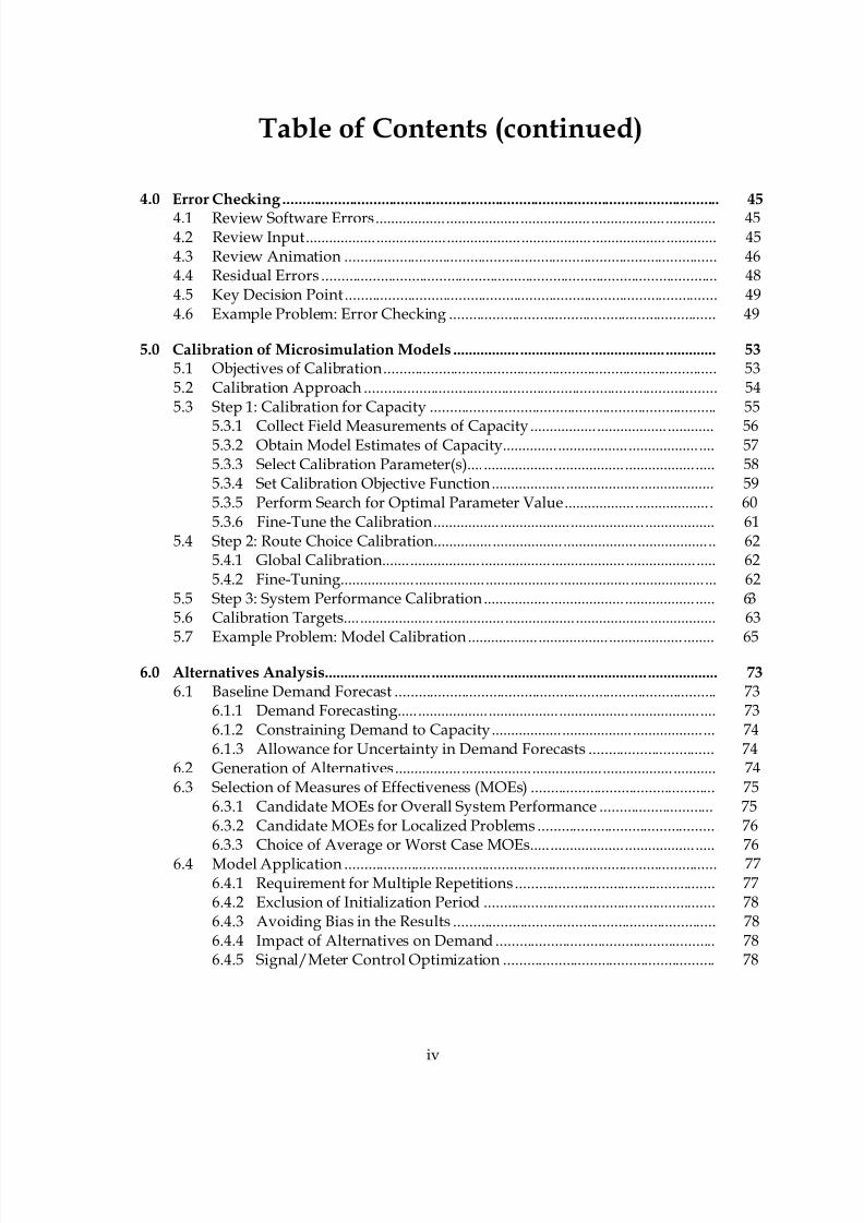
4.0 Error Checking ............................................................................................................... 45
4.1 Review Software Errors....................................................................................... 454.2 Review Input......................................................................................................... 454.3 Review Animation ............................................................................................... 464.4 Residual Errors ..................................................................................................... 484.5 Key Decision Point............................................................................................... 494.6 Example Problem: Error Checking .................................................................... 49
5.0 Calibration of Microsimulation Models ................................................................... 535.1 Objectives of Calibration..................................................................................... 535.2 Calibration Approach .......................................................................................... 545.3 Step 1: Calibration for Capacity ......................................................................... 55
5.3.1 Collect Field Measurements of Capacity ............................................... 565.3.2 Obtain Model Estimates of Capacity...................................................... 575.3.3 Select Calibration Parameter(s)............................................................... 585.3.4 Set Calibration Objective Function......................................................... 595.3.5 Perform Search for Optimal Parameter Value...................................... 605.3.6 Fine-Tune the Calibration........................................................................ 61
5.4 Step 2: Route Choice Calibration........................................................................ 625.4.1 Global Calibration..................................................................................... 625.4.2 Fine-Tuning................................................................................................ 62
5.5 Step 3: System Performance Calibration........................................................... 63 5.6 Calibration Targets............................................................................................... 63
5.7 Example Problem: Model Calibration............................................................... 65
6.0 Alternatives Analysis.................................................................................................... 736.1 Baseline Demand Forecast .................................................................................. 73
6.1.1 Demand Forecasting................................................................................. 736.1.2 Constraining Demand to Capacity......................................................... 746.1.3 Allowance for Uncertainty in Demand Forecasts ................................ 74
6.2 Generation of Alternatives.................................................................................. 746.3 Selection of Measures of Effectiveness (MOEs) ............................................... 75
6.3.1 Candidate MOEs for Overall System Performance ............................. 756.3.2 Candidate MOEs for Localized Problems ............................................. 766.3.3 Choice of Average or Worst Case MOEs............................................... 76
6.4 Model Application ............................................................................................... 776.4.1 Requirement for Multiple Repetitions................................................... 776.4.2 Exclusion of Initialization Period ........................................................... 786.4.3 Avoiding Bias in the Results ................................................................... 786.4.4 Impact of Alternatives on Demand ........................................................ 786.4.5 Signal/Meter Control Optimization ...................................................... 78
8/8/2019 Vol3 Guidelines
http://slidepdf.com/reader/full/vol3-guidelines 7/146
v
Table of Contents (continued)
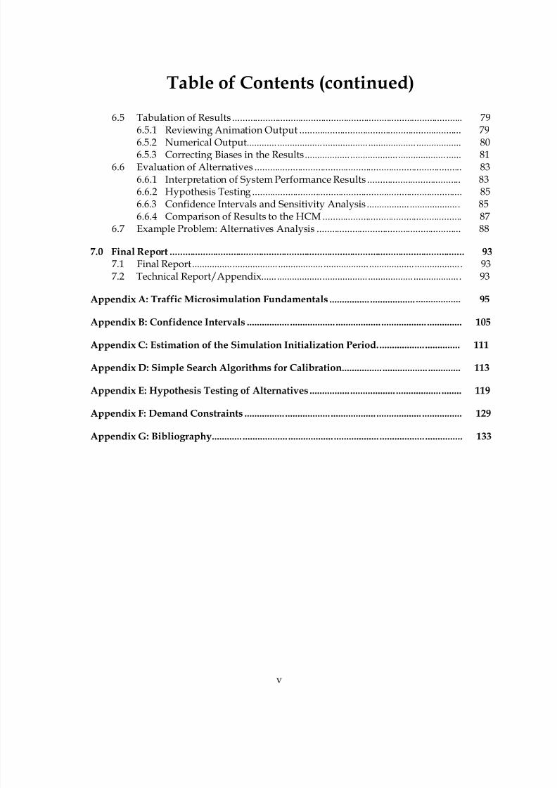
6.5 Tabulation of Results ........................................................................................... 796.5.1 Reviewing Animation Output ................................................................ 796.5.2 Numerical Output..................................................................................... 806.5.3 Correcting Biases in the Results.............................................................. 81
6.6 Evaluation of Alternatives .................................................................................. 836.6.1 Interpretation of System Performance Results ..................................... 836.6.2 Hypothesis Testing ................................................................................... 856.6.3 Confidence Intervals and Sensitivity Analysis ..................................... 856.6.4 Comparison of Results to the HCM ....................................................... 87
6.7 Example Problem: Alternatives Analysis ......................................................... 88
7.0 Final Report .................................................................................................................... 937.1 Final Report........................................................................................................... 93
7.2 Technical Report/Appendix............................................................................... 93
Appendix A: Traffic Microsimulation Fundamentals .................................................... 95
Appendix B: Confidence Intervals ..................................................................................... 105
Appendix C: Estimation of the Simulation Initialization Period................................. 111
Appendix D: Simple Search Algorithms for Calibration............................................... 113
Appendix E: Hypothesis Testing of Alternatives ............................................................ 119
Appendix F: Demand Constraints ...................................................................................... 129
Appendix G: Bibliography................................................................................................... 133
8/8/2019 Vol3 Guidelines
http://slidepdf.com/reader/full/vol3-guidelines 8/146
vi
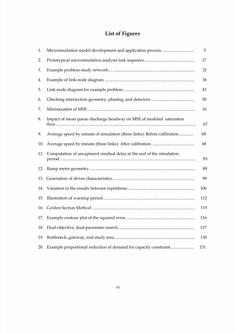
List of Figures
1. Microsimulation model development and application process. ............................. 5
2. Prototypical microsimulation analysis task sequence............................................... 17
3. Example problem study network................................................................................. 21
4. Example of link-node diagram. .................................................................................... 36
5. Link-node diagram for example problem................................................................... 43
6. Checking intersection geometry, phasing, and detectors. ........................................ 50
7. Minimization of MSE..................................................................................................... 61
8. Impact of mean queue discharge headway on MSE of modeled saturationflow................................................................................................................................... 67
9. Average speed by minute of simulation (three links): Before calibration. ............. 68
10. Average speed by minute (three links): After calibration. ....................................... 68
11. Computation of uncaptured residual delay at the end of the simulationperiod. .............................................................................................................................. 83
12. Ramp meter geometry. .................................................................................................. 89
13. Generation of driver characteristics. ............................................................................ 99
14. Variation in the results between repetitions. .............................................................. 106
15. Illustration of warmup period. ..................................................................................... 112
16. Golden Section Method. ................................................................................................ 115
17. Example contour plot of the squared error................................................................. 116
18. Dual-objective, dual-parameter search........................................................................ 117
19. Bottleneck, gateway, and study area. .......................................................................... 130
20. Example proportional reduction of demand for capacity constraint...................... 131
8/8/2019 Vol3 Guidelines
http://slidepdf.com/reader/full/vol3-guidelines 9/146
vii
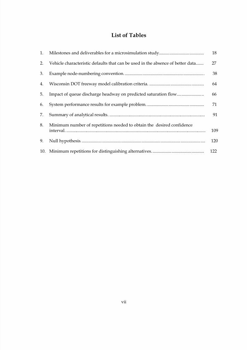
List of Tables
1. Milestones and deliverables for a microsimulation study........................................ 18
2. Vehicle characteristic defaults that can be used in the absence of better data....... 27
3. Example node-numbering convention. ....................................................................... 38
4. Wisconsin DOT freeway model calibration criteria. ................................................. 64
5. Impact of queue discharge headway on predicted saturation flow........................ 66
6. System performance results for example problem. ................................................... 71
7. Summary of analytical results. ..................................................................................... 91
8. Minimum number of repetitions needed to obtain the desired confidenceinterval. ............................................................................................................................ 109
9. Null hypothesis............................................................................................................... 120
10. Minimum repetitions for distinguishing alternatives. .............................................. 122

8/8/2019 Vol3 Guidelines
http://slidepdf.com/reader/full/vol3-guidelines 10/146
8/8/2019 Vol3 Guidelines
http://slidepdf.com/reader/full/vol3-guidelines 11/146
1
Introduction
Microsimulation is the modeling of individual vehicle movements on a second or subsecond
basis for the purpose of assessing the traffic performance of highway and street systems,transit, and pedestrians. The last few years have seen a rapid evolution in thesophistication of microsimulation models and a major expansion of their use intransportation engineering and planning practices. These guidelines provide practitionerswith guidance on the appropriate application of microsimulation models to traffic analysisproblems, with an overarching focus on existing and future alternatives analysis.
The use of these guidelines will aid in the consistent and reproducible application ofmicrosimulation models and will further support the credibility of the tools of today andtomorrow. As a result, practitioners and decisionmakers will be equipped to makeinformed decisions that will account for current and evolving technology. Depending onthe project-specific purpose, need, and scope, elements of the process described in theseguidelines may be enhanced or adapted to support the analyst and the project team. It isstrongly recommended that the respective stakeholders and partners consult prior to andthroughout the application of any microsimulation model. This further supports thecredibility of the results, recommendations, and conclusions, and minimizes the potentialfor unnecessary or unanticipated tasks.
Organization of Guidelines
These guidelines are organized into the following chapters and appendixes:
Introduction (this chapter) highlights the key guiding principles of microsimulation andprovides an overview of these guidelines.
Chapter 1.0 addresses the management, scope, and organization of microsimulationanalyses.
Chapter 2.0 discusses the steps necessary to collect and prepare input data for use inmicrosimulation models.
Chapter 3.0 discusses the coding of input data into the microsimulation models.
Chapter 4.0 presents error-checking methods.
Chapter 5.0 provides guidance on the calibration of microsimulation models to localtraffic conditions.
8/8/2019 Vol3 Guidelines
http://slidepdf.com/reader/full/vol3-guidelines 12/146
2
Chapter 6.0 explains how to use microsimulation models for alternatives analysis.
Chapter 7.0 provides guidance on the documentation of microsimulation model analysis.
Appendix A provides an introduction to the fundamentals of microsimulation model
theory.
Appendix B provides guidance on the estimation of the minimum number ofmicrosimulation model run repetitions necessary for achieving a target confidence leveland confidence interval.
Appendix C provides guidance on the estimation of the duration of the initialization(warmup) period, after which the simulation has stabilized and it is then appropriate tobegin gathering performance statistics.
Appendix D provides examples of some simple manual search algorithms for optimizingparameters during calibration.
Appendix E summarizes the standard statistical tests that can be used to determinewhether two alternatives result in significantly different performance. The purpose ofthese tests is to demonstrate that the improved performance in a particular alternative isnot a result of random variation in the simulation model results.
Appendix F describes a manual method for constraining external demands to availablecapacity. This method is useful for adapting travel demand model forecasts for use inmicrosimulation models.
Appendix G provides useful references on microsimulation.
Guiding Principles of Microsimulation
Microsimulation can provide the analyst with valuable information on the performance ofthe existing transportation system and potential improvements. However,microsimulation can also be a time-consuming and resource-intensive activity. The key toobtaining a cost-effective microsimulation analysis is to observe certain guiding principlesfor this type of analysis:
• Use of the appropriate tool is essential. Do not use microsimulation analysis when it isnot appropriate. Understand the limitations of the tool and ensure that it accurately
represents the traffic operations theory. Confirm that it can be applied to support thepurpose, needs, and scope of work, and can address the question that is being asked.

8/8/2019 Vol3 Guidelines
http://slidepdf.com/reader/full/vol3-guidelines 13/146
3
• Traffic Analysis Toolbox, Volume II: Decision Support Methodology for Selecting Traffic Analysis Tools (Federal Highway Administration (FHWA), presents a methodology forselecting the appropriate type of traffic analysis tool for the task.
• Do not use microsimulation if sufficient time and resources are not available.
Misapplication can degrade credibility and can be a focus of controversy ordisagreement.
• Good data are critical for good microsimulation model results.
• It is critical that the analyst calibrate any microsimulation model to local conditions.
• Output of a microsimulation model is different from that of the Highway Capacity Manual (HCM) (Transportation Research Board (TRB)). Definitions of key terms, suchas “delay” and “queues,” are different at the microscopic level of microsimulationmodels than at the macroscopic level typical of the HCM.
• Prior to embarking on the development of a microsimulation model, establish itsscope among the partners, taking into consideration expectations, tasks, and anunderstanding of how the tool will support the engineering decision. Identify knownlimitations.
• To minimize disagreements between partners, embed interim periodic reviews atprudent milestones in the model development and calibration processes.
Additional information on traffic microsimulation fundamentals is provided in appendix A.
Terminology Used in These Guidelines
Calibration: Process where the analyst selects the model parameters that cause the modelto best reproduce field-measured local traffic operations conditions.
Microsimulation: Modeling of individual vehicle movements on a second or subsecondbasis for the purpose of assessing the traffic performance of highway and street systems.
Model: Specific combination of modeling software and analyst-developed input/parameters for a specific application. A single model may be applied to the same study
area for several time periods and several existing and future improvement alternatives.
Project: To reduce the chances of confusing the analysis of a project with the project itself,this report limits the use of the term “project” to the physical road improvement beingstudied. The evaluation of the impact of a project will be called an “analysis.”

8/8/2019 Vol3 Guidelines
http://slidepdf.com/reader/full/vol3-guidelines 14/146
4
Software: Set of computer instructions for assisting the analyst in the development andapplication of a specific microsimulation model. Several models can be developed using asingle software program. These models will share the same basic computationalalgorithms embedded in the software; however, they will employ different input andparameter values.
Validation: Process where the analyst checks the overall model-predicted trafficperformance for a street/road system against field measurements of traffic performance,such as traffic volumes, travel times, average speeds, and average delays. Modelvalidation is performed based on field data not used in the calibration process. This reportpresumes that the software developer has already completed this validation of thesoftware and its underlying algorithms in a number of research and practical applications.
Verification: Process where the software developer and other researchers check theaccuracy of the software implementation of traffic operations theory. This report providesno information on software verification procedures.
Microsimulation Model Development and Application Process
The overall process for developing and applying a microsimulation model to a specifictraffic analysis problem consists of seven major tasks:
1. Identification of Study Purpose, Scope, and Approach.
2. Data Collection and Preparation.
3. Base Model Development.
4. Error Checking.
5. Calibration.
6. Alternatives Analysis.
7. Final Report and Technical Documentation.
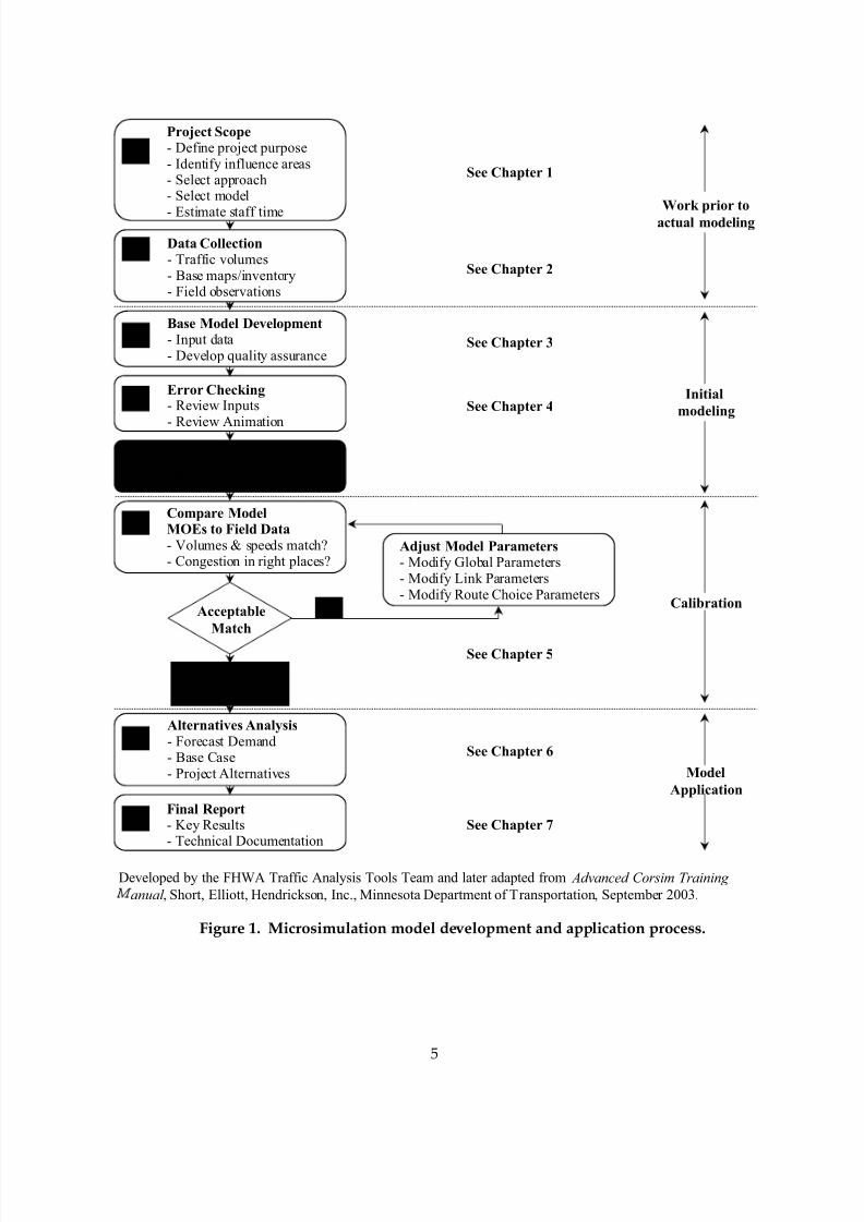
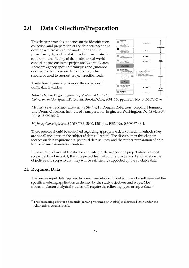
Each task is summarized below and described in more detail in subsequent chapters. Aflow chart, complementing the overall process, is presented in figure 1. It is intended to bea quick reference that will be traceable throughout the document. This report’s chapters
correspond to the numbering scheme in figure 1.
8/8/2019 Vol3 Guidelines
http://slidepdf.com/reader/full/vol3-guidelines 15/146
5
No
Data Collection- Traffic volumes- Base maps/inventory- Field observations
2
1
Project Scope- Define project purpose- Identify influence areas- Select approach- Select model
- Estimate staff time
See Chapter 1
See Chapter 2
See Chapter 3
See Chapter 4
Work prior to
actual modeling
Initial
modeling
Yes
Calibrated Model
See Chapter 5
Calibration
See Chapter 6
See Chapter 7
Model
Application
Base Model Development- Input data- Develop quality assurance
3
Error Checking- Review Inputs
- Review Animation
4
Compare ModelMOEs to Field Data
- Volumes & speeds match?- Congestion in right places?
5
Alternatives Analysis
- Forecast Demand- Base Case- Project Alternatives
6
Final Report- Key Results- Technical Documentation
7
Working Model
Before Calibration
Acceptable
Match
Adjust Model Parameters- Modify Global Parameters- Modify Link Parameters- Modify Route Choice Parameters
Developed by the FHWA Traffic Analysis Tools Team and later adapted from Advanced Corsim Training
anual , Short, Elliott, Hendrickson, Inc., Minnesota Department of Transportation, September 2003.
Figure 1. Microsimulation model development and application process.

8/8/2019 Vol3 Guidelines
http://slidepdf.com/reader/full/vol3-guidelines 16/146
6
To demonstrate the process, an example problem is also provided. The example probleminvolves the analysis of a corridor consisting of a freeway section and a parallel arterial.For simplicity, this example assumes a proactive traffic management strategy thatincludes ramp metering. Realizing that each project is unique, the analyst and projectmanager may see a need to revisit previous tasks in the process to fully address the issues
that arise.
Organization and management of a microsimulation analysis require the development ofa “scope” for the analysis. This scope includes identification of project objectives, availableresources, assessment of verified and available tools, quality assurance plan, andidentification of the appropriate tasks to complete the analysis.
Task 1: Microsimulation Analysis Organization/Scope
The key issues for the management of a microsimulation study are:
• Securing sufficient expertise to develop and/or evaluate the model.
• Providing sufficient time and resources to develop and calibrate the microsimulationmodel.
• Developing adequate documentation for the model development process andcalibration results.
Task 2: Data Collection and Preparation
This task involves the collection and preparation of all of the data necessary for themicrosimulation analysis. Microsimulation models require extensive input data, including:
• Geometry (lengths, lanes, curvature).
• Controls (signal timing, signs).
• Existing demands (turning volumes, origin-destination (O-D) table).
• Calibration data (capacities, travel times, queues).
• Transit, bicycle, and pedestrian data.
In support of tasks 4 and 5, the current and accurate data required for error checking andcalibration should also be collected. While capacities can be measured at any time, it is
crucial that the other calibration data (travel times, delays, and queues) be gatheredsimultaneously with the traffic counts.
8/8/2019 Vol3 Guidelines
http://slidepdf.com/reader/full/vol3-guidelines 17/146
7
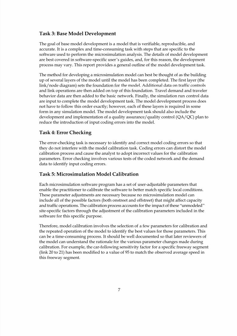
Task 3: Base Model Development
The goal of base model development is a model that is verifiable, reproducible, andaccurate. It is a complex and time-consuming task with steps that are specific to thesoftware used to perform the microsimulation analysis. The details of model development
are best covered in software-specific user’s guides, and, for this reason, the developmentprocess may vary. This report provides a general outline of the model development task.
The method for developing a microsimulation model can best be thought of as the buildingup of several layers of the model until the model has been completed. The first layer (thelink/node diagram) sets the foundation for the model. Additional data on traffic controlsand link operations are then added on top of this foundation. Travel demand and travelerbehavior data are then added to the basic network. Finally, the simulation run control dataare input to complete the model development task. The model development process doesnot have to follow this order exactly; however, each of these layers is required in someform in any simulation model. The model development task should also include the
development and implementation of a quality assurance/quality control (QA/QC) plan toreduce the introduction of input coding errors into the model.
Task 4: Error Checking
The error-checking task is necessary to identify and correct model coding errors so thatthey do not interfere with the model calibration task. Coding errors can distort the modelcalibration process and cause the analyst to adopt incorrect values for the calibrationparameters. Error checking involves various tests of the coded network and the demanddata to identify input coding errors.
Task 5: Microsimulation Model CalibrationEach microsimulation software program has a set of user-adjustable parameters thatenable the practitioner to calibrate the software to better match specific local conditions.These parameter adjustments are necessary because no microsimulation model caninclude all of the possible factors (both onstreet and offstreet) that might affect capacityand traffic operations. The calibration process accounts for the impact of these “unmodeled” site-specific factors through the adjustment of the calibration parameters included in thesoftware for this specific purpose.
Therefore, model calibration involves the selection of a few parameters for calibration andthe repeated operation of the model to identify the best values for those parameters. This
can be a time-consuming process. It should be well documented so that later reviewers ofthe model can understand the rationale for the various parameter changes made duringcalibration. For example, the car-following sensitivity factor for a specific freeway segment(link 20 to 21) has been modified to a value of 95 to match the observed average speed inthis freeway segment.
8/8/2019 Vol3 Guidelines
http://slidepdf.com/reader/full/vol3-guidelines 18/146
8
The key issues in calibration are:
• Identification of necessary model calibration targets.
• Allocation of sufficient time and resources to achieve calibration targets.
• Selection of the appropriate calibration parameter values to best match locallymeasured street, highway, freeway, and intersection capacities.
• Selection of the calibration parameter values that best reproduce current route choicepatterns.
• Calibration of the overall model against overall system performance measures, suchas travel time, delay, and queues.
Task 6: Alternatives Analysis With Microsimulation Models
This is the first model application task. The calibrated microsimulation model is runseveral times to test various project alternatives. The first step in this task is to develop abaseline demand scenario. Then the various improvement alternatives are coded into thesimulation model. The analyst then determines which performance statistics will begathered and runs the model for each alternative to generate the necessary output. If theanalyst wishes to produce HCM level-of-service (LOS) results, then sufficient time shouldbe allowed for post-processing the model output to convert microsimulation results intoHCM-compatible LOS results.
The key issues in an alternatives analysis are:
• Forecasting realistic future demands.
• Selecting the appropriate performance measures for evaluation of the alternatives.
• Accurate accounting of the full congestion-reduction benefits of each alternative.
• Properly converting the microsimulation results to HCM LOS (reporting LOS isoptional).
Task 7: Final Report/Technical Documentation
This task involves summarizing the analytical results in a final report and documentingthe analytical approach in a technical document. This task may also include presentationof study results to technical supervisors, elected officials, and the general public.
The final report presents the analytical results in a form that is readily understandable bythe decisionmakers for the project. The effort involved in summarizing the results for the

8/8/2019 Vol3 Guidelines
http://slidepdf.com/reader/full/vol3-guidelines 19/146
9
final report should not be underestimated, since microsimulation models produce awealth of numerical output that must be tabulated and summarized.
Technical documentation is important for ensuring that the decisionmakers understandthe assumptions behind the results and for enabling other analysts to reproduce the
results. The documentation should be sufficient so that given the same input files, anotheranalyst can understand the calibration process and repeat the alternatives analysis.

8/8/2019 Vol3 Guidelines
http://slidepdf.com/reader/full/vol3-guidelines 20/146
8/8/2019 Vol3 Guidelines
http://slidepdf.com/reader/full/vol3-guidelines 21/146
11
No
Data Collection
- Traffic volumes- Base maps/inventory- Field observations
2
1
Project Scope
- Define project purpose- Identify influence areas
- Select approach- Select model- Estimate staff time
See Chapter 1
See Chapter 2
See Chapter 3
See Chapter 4
Work prior to
actual modeling
Initial
modeling
Yes
Calibrated Model
See Chapter 5
Calibration
See Chapter 6
See Chapter 7
Model
Application
Base Model Development
- Input data- Develop qualityassurance
3
Error Checking
- Review Inputs- Review Animation
4
Compare Model
MOEs to Field Data
- Volumes & speedsmatch?- Congestion in right places?
5
Alternatives Analysis
- Forecast Demand- Base Case- Project Alternatives
6
Final Report
- Key Results
- Technical Documentation
7
Working Model
Before Calibration
Acceptable
Match
Adjust Model Parameters
- Modify Global Parameters- Modify Link Parameters- Modify Route Choice Parameters
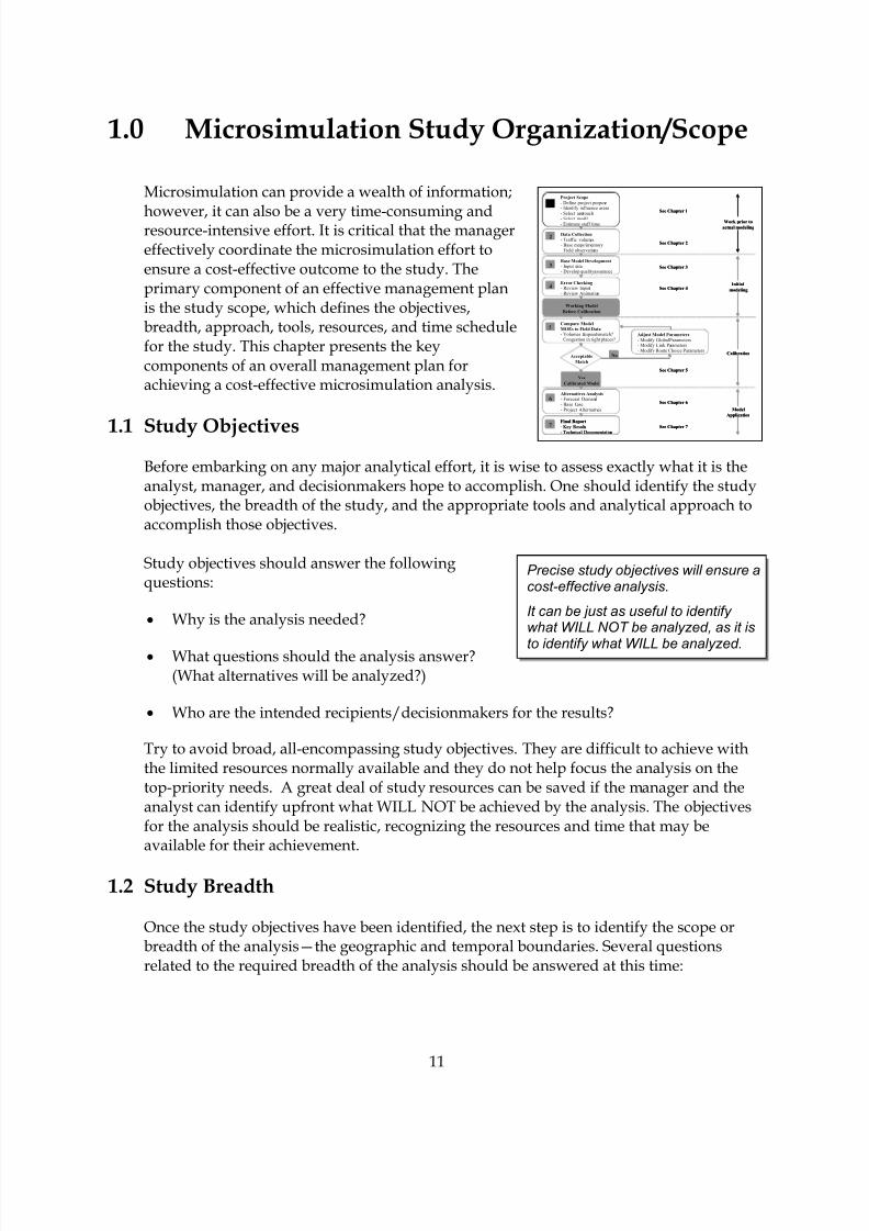
1.0 Microsimulation Study Organization/Scope
Microsimulation can provide a wealth of information;
however, it can also be a very time-consuming andresource-intensive effort. It is critical that the managereffectively coordinate the microsimulation effort toensure a cost-effective outcome to the study. Theprimary component of an effective management planis the study scope, which defines the objectives,breadth, approach, tools, resources, and time schedulefor the study. This chapter presents the keycomponents of an overall management plan forachieving a cost-effective microsimulation analysis.
1.1 Study Objectives
Before embarking on any major analytical effort, it is wise to assess exactly what it is theanalyst, manager, and decisionmakers hope to accomplish. One should identify the studyobjectives, the breadth of the study, and the appropriate tools and analytical approach toaccomplish those objectives.
Study objectives should answer the followingquestions:
• Why is the analysis needed?
• What questions should the analysis answer?(What alternatives will be analyzed?)
• Who are the intended recipients/decisionmakers for the results?
Try to avoid broad, all-encompassing study objectives. They are difficult to achieve withthe limited resources normally available and they do not help focus the analysis on thetop-priority needs. A great deal of study resources can be saved if the manager and theanalyst can identify upfront what WILL NOT be achieved by the analysis. The objectivesfor the analysis should be realistic, recognizing the resources and time that may beavailable for their achievement.
1.2 Study Breadth
Once the study objectives have been identified, the next step is to identify the scope orbreadth of the analysis—the geographic and temporal boundaries. Several questionsrelated to the required breadth of the analysis should be answered at this time:
Precise study objectives will ensure acost-effective analysis.
It can be just as useful to identify what WILL NOT be analyzed, as it is
to identify what WILL be analyzed.

8/8/2019 Vol3 Guidelines
http://slidepdf.com/reader/full/vol3-guidelines 22/146
12
• What are the characteristics of the project being analyzed? How large and complex isit?
• What are the alternatives to be analyzed? How many of them are there? How large
and complex are they?
• What measures of effectiveness (MOEs) will be required to evaluate the alternativesand how can they be measured in the field?
• What resources are available to the analyst?
• What are the probable geographic and temporalscopes of the impact of the project and itsalternatives (now and in the future)? How farand for how many hours does the congestion
extend? The geographic and temporalboundaries selected for the analysis shouldencompass all of the expected congestion toprovide a valid basis for comparingalternatives.1
• What degree of precision do the decisionmakers require? Is a 10-percent errortolerable? Are hourly averages satisfactory? Will the impact of the alternatives be verysimilar or very different from those of the proposed project? How disaggregate ananalysis is required? Is the analysis likely to produce a set of alternatives where thedecisionmakers must choose between varying levels of congestion (as opposed to asituation where one or more alternatives eliminate congestion, while others do not)?
Development of a logical terminus of an improvement project versus a model has beendebated since the early days of microsimulation; in the end, it is a matter of balancingstudy objectives and study resources. Therefore, the modeler needs to understand theoperation of the improvement project to develop logical termini.
The study termini will be dependent on the “zone of influence,” and the project managerwill probably make that determination in consultation with the project stakeholders. Once
1 The analyst should try to design the model to geographically and temporally encompass all
significant congestion to ensure that the model is evaluating demands rather than capacity;however, the extent of the congestion in many urban areas and resource limitations may preclude100 percent achievement of this goal. If this goal cannot be achieved 100 percent, then the analystshould attempt to encompass as much of the congestion as is feasible within the resourceconstraints and be prepared to post-process the model’s results to compensate for the portion ofcongestion not included in the model.
The geographic and temporal scopesof a microsimulation model should besufficient to completely encompass all of the traffic congestion present in the
primary influence area of the project during the target analysis period.

8/8/2019 Vol3 Guidelines
http://slidepdf.com/reader/full/vol3-guidelines 23/146
13
that has been completed, the modeler then needs to look at the operation of the proposedfacility. When determining the zone of influence, the modeler needs to understand theoperational characteristics of the facility in the proposed project. This could be oneintersection beyond the project terminus at one end of the project or a major generator 3.2kilometers (km) (2 miles (mi)) away from the other end of the project. Therefore, there is
no geographical guidance that can be given. However, some general guidelines can besummarized as follows:
Interstate Projects: The model network should extend up to 2.4 km (1.5 mi) from bothtermini of the improvement being evaluated and up to 1.6 km (1 mi) on either side of theinterstate route. This will allow sufficient time and distance for the model to betterdevelop the traffic-stream characteristics reflected in the real world.
Arterial Projects: The model network should extend at least one intersection beyond thosewithin the boundaries of the improvement and should consider the potential impact onarterial coordination as warranted. This will capture influences such as the upstream
metering of traffic and the downstream queuing of traffic.
The model study area should include areas that might be impacted by the proposedimprovement strategies. For example, if an analysis is to be conducted of incidentmanagement strategies, the model study area should include the area impacted by thediverted traffic. All potential problem areas should be included in the model network. Forexample, if queues are identified in the network boundary areas, the analyst might need toextend the network further upstream.
A study scope that has a tight geographic focus,little tolerance for error, and little difference in theperformance of the alternatives will tend to point to
microsimulation as the most cost-effectiveapproach.2 A scope with a moderately greatergeographic focus and with a timeframe 20 years inthe future will tend to require a blended traveldemand model and microsimulation approach. A scope that covers large geographic areasand long timeframes in the future will tend to rule out microsimulation and will insteadrequire a combination of travel demand models and HCM analytical techniques.
2 Continuing improvements in data collection, computer technology, and software will eventuallyenable microsimulation models to be applied to larger problems.
Microsimulation is like a microscope.It is a very effective tool when you have it pointed at the correct subject.Tightly focused scopes of work ensure cost-effective microsimulationanalyses.
8/8/2019 Vol3 Guidelines
http://slidepdf.com/reader/full/vol3-guidelines 24/146
14
1.3 Analytical Approach Selection
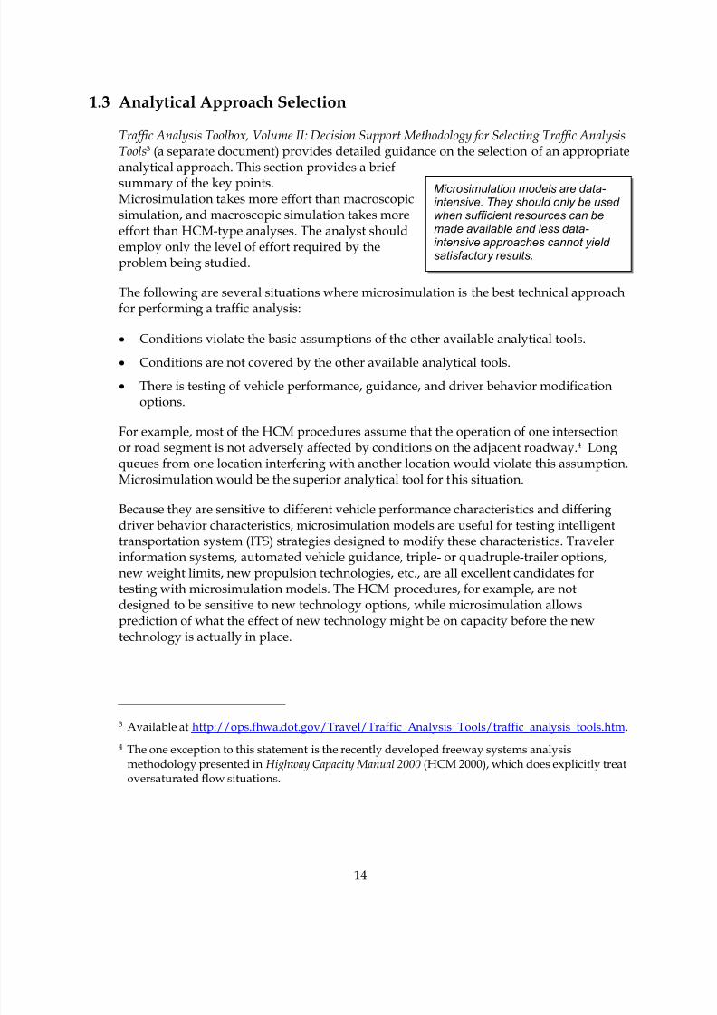
Traffic Analysis Toolbox, Volume II: Decision Support Methodology for Selecting Traffic AnalysisTools3 (a separate document) provides detailed guidance on the selection of an appropriateanalytical approach. This section provides a briefsummary of the key points.Microsimulation takes more effort than macroscopicsimulation, and macroscopic simulation takes moreeffort than HCM-type analyses. The analyst shouldemploy only the level of effort required by theproblem being studied.
The following are several situations where microsimulation is the best technical approachfor performing a traffic analysis:
• Conditions violate the basic assumptions of the other available analytical tools.
• Conditions are not covered by the other available analytical tools.
• There is testing of vehicle performance, guidance, and driver behavior modificationoptions.
For example, most of the HCM procedures assume that the operation of one intersectionor road segment is not adversely affected by conditions on the adjacent roadway.4 Longqueues from one location interfering with another location would violate this assumption.Microsimulation would be the superior analytical tool for this situation.
Because they are sensitive to different vehicle performance characteristics and differingdriver behavior characteristics, microsimulation models are useful for testing intelligenttransportation system (ITS) strategies designed to modify these characteristics. Travelerinformation systems, automated vehicle guidance, triple- or quadruple-trailer options,new weight limits, new propulsion technologies, etc., are all excellent candidates fortesting with microsimulation models. The HCM procedures, for example, are notdesigned to be sensitive to new technology options, while microsimulation allowsprediction of what the effect of new technology might be on capacity before the newtechnology is actually in place.
3 Available at http://ops.fhwa.dot.gov/Travel/Traffic_Analysis_Tools/traffic_analysis_tools.htm.
4 The one exception to this statement is the recently developed freeway systems analysismethodology presented in Highway Capacity Manual 2000 (HCM 2000), which does explicitly treatoversaturated flow situations.
Microsimulation models are data-intensive. They should only be used when sufficient resources can bemade available and less data-intensive approaches cannot yield satisfactory results.
8/8/2019 Vol3 Guidelines
http://slidepdf.com/reader/full/vol3-guidelines 25/146
15
Software selection is like picking out asuit of clothes. There is no single suit
that fits all people and all uses. You must know what your software needsare and the capabilities and training of the people that you expect to use thesoftware. Then you can select thesoftware that best meets your needsand best fits the capabilities of the
people who will use it.
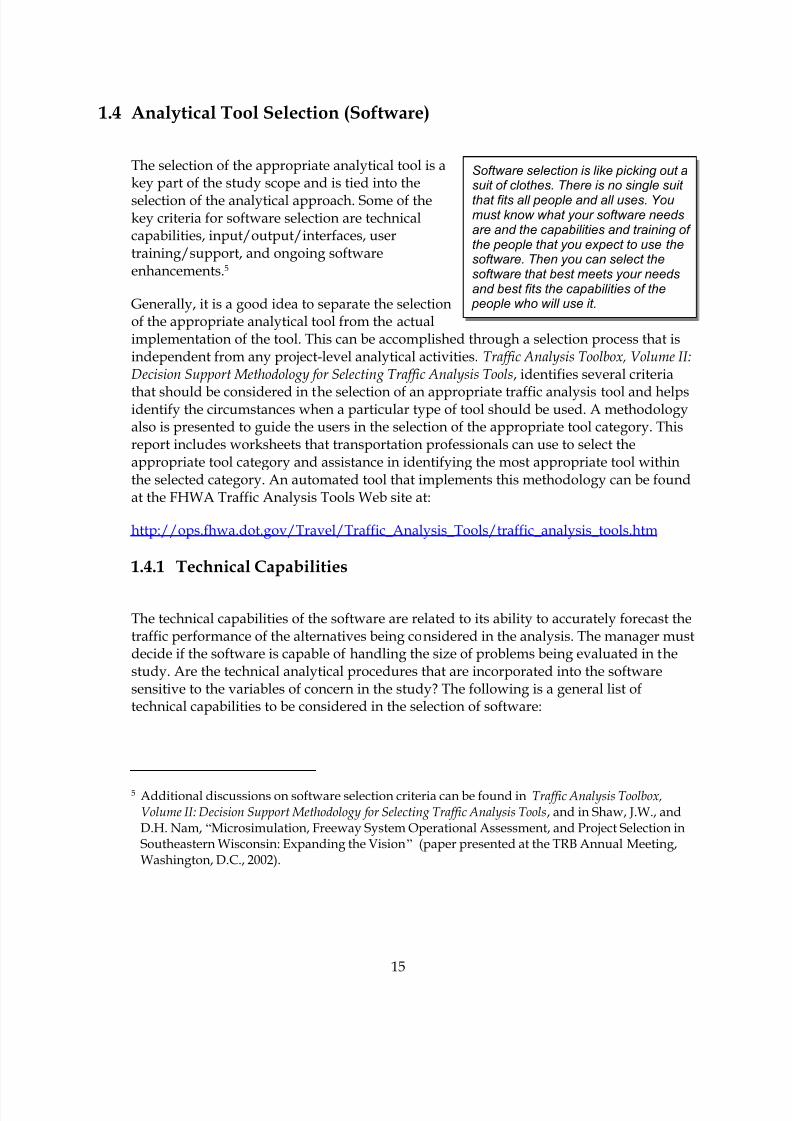
1.4 Analytical Tool Selection (Software)
The selection of the appropriate analytical tool is akey part of the study scope and is tied into the
selection of the analytical approach. Some of thekey criteria for software selection are technicalcapabilities, input/output/interfaces, usertraining/support, and ongoing softwareenhancements.5
Generally, it is a good idea to separate the selectionof the appropriate analytical tool from the actualimplementation of the tool. This can be accomplished through a selection process that isindependent from any project-level analytical activities. Traffic Analysis Toolbox, Volume II:Decision Support Methodology for Selecting Traffic Analysis Tools, identifies several criteria
that should be considered in the selection of an appropriate traffic analysis tool and helpsidentify the circumstances when a particular type of tool should be used. A methodologyalso is presented to guide the users in the selection of the appropriate tool category. Thisreport includes worksheets that transportation professionals can use to select theappropriate tool category and assistance in identifying the most appropriate tool withinthe selected category. An automated tool that implements this methodology can be foundat the FHWA Traffic Analysis Tools Web site at:
http://ops.fhwa.dot.gov/Travel/Traffic_Analysis_Tools/traffic_analysis_tools.htm
1.4.1 Technical Capabilities
The technical capabilities of the software are related to its ability to accurately forecast thetraffic performance of the alternatives being considered in the analysis. The manager mustdecide if the software is capable of handling the size of problems being evaluated in thestudy. Are the technical analytical procedures that are incorporated into the softwaresensitive to the variables of concern in the study? The following is a general list oftechnical capabilities to be considered in the selection of software:
5 Additional discussions on software selection criteria can be found in Traffic Analysis Toolbox,Volume II: Decision Support Methodology for Selecting Traffic Analysis Tools, and in Shaw, J.W., andD.H. Nam, “Microsimulation, Freeway System Operational Assessment, and Project Selection inSoutheastern Wisconsin: Expanding the Vision” (paper presented at the TRB Annual Meeting,Washington, D.C., 2002).
8/8/2019 Vol3 Guidelines
http://slidepdf.com/reader/full/vol3-guidelines 26/146
16
• Maximum problem size (the software may be limited by the maximum number ofsignals that can be in a single network or the maximum number of vehicles that maybe present on the network at any one time).
• Vehicle movement logic (lane changing, car following, etc.) that reflects the state of the
art.
• Sensitivity to specific features of the alternatives being analyzed (such as trucks ongrades, effects of horizontal curvature on speeds, or advanced traffic managementtechniques).
• Model parameters available for model calibration.
• Variety and extent of prior successful applications of the software program (should beconsidered by the manager).
1.4.2 Input/Output/Interfaces
Input, output, and the ability of the software to interface with other software that will beused in the study (such as traffic forecasting models) are other key considerations. Themanager should review the ability of the software to produce reports on the MOEs neededfor the study. The ability to customize output reports can also be very useful to the analyst.It is essential that the manager or analyst understand the definitions of the MOEs asdefined by the software. This is because a given MOE may be calculated or defineddifferently by the software in comparison to how it is defined or calculated by the HCM.
1.4.3 User Training/Support
User training and support requirements are another key consideration. What kind oftraining and support is available? Are there other users in the area that can provideinformal advice?
1.4.4 Ongoing Software Enhancements
Finally, the commitment of the software developer to ongoing enhancements ensures thatthe agency’s investment in staff training and model development for a particular softwaretool will continue to pay off over the long term. Unsupported software can becomeunusable if improvements are made to operating systems and hardware.
1.5 Resource Requirements
The resource requirements for the development, calibration, and application ofmicrosimulation models will vary according to the complexity of the project, its
8/8/2019 Vol3 Guidelines
http://slidepdf.com/reader/full/vol3-guidelines 27/146
17
geographic scope, temporal scope, number of alternatives, and the availability and qualityof the data.6 In terms of training, the person responsible for the initial round of coding can be abeginner or on an intermediate level in terms of knowledge of the software. They shouldhave supervision from an individual with more experience with the software. Error
checking and calibration are best done by a person with advanced knowledge ofmicrosimulation software and the underlying algorithms. Model documentation andpublic presentations can be done by a person with an intermediate level of knowledge ofmicrosimulation software.
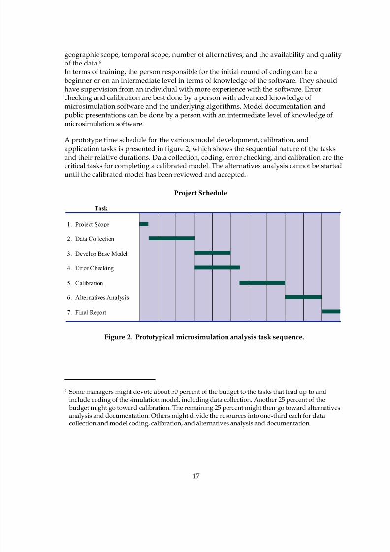
A prototype time schedule for the various model development, calibration, andapplication tasks is presented in figure 2, which shows the sequential nature of the tasksand their relative durations. Data collection, coding, error checking, and calibration are thecritical tasks for completing a calibrated model. The alternatives analysis cannot be starteduntil the calibrated model has been reviewed and accepted.
Task
1. Project Scope
2. Data Collection
3. Develop Base Model
4. Error Checking
5. Calibration
6. Alternatives Analysis
7. Final Report
Project Schedule
Figure 2. Prototypical microsimulation analysis task sequence.
6 Some managers might devote about 50 percent of the budget to the tasks that lead up to andinclude coding of the simulation model, including data collection. Another 25 percent of thebudget might go toward calibration. The remaining 25 percent might then go toward alternativesanalysis and documentation. Others might divide the resources into one-third each for datacollection and model coding, calibration, and alternatives analysis and documentation.
8/8/2019 Vol3 Guidelines
http://slidepdf.com/reader/full/vol3-guidelines 28/146
18
1.6 Management of a Microsimulation Study
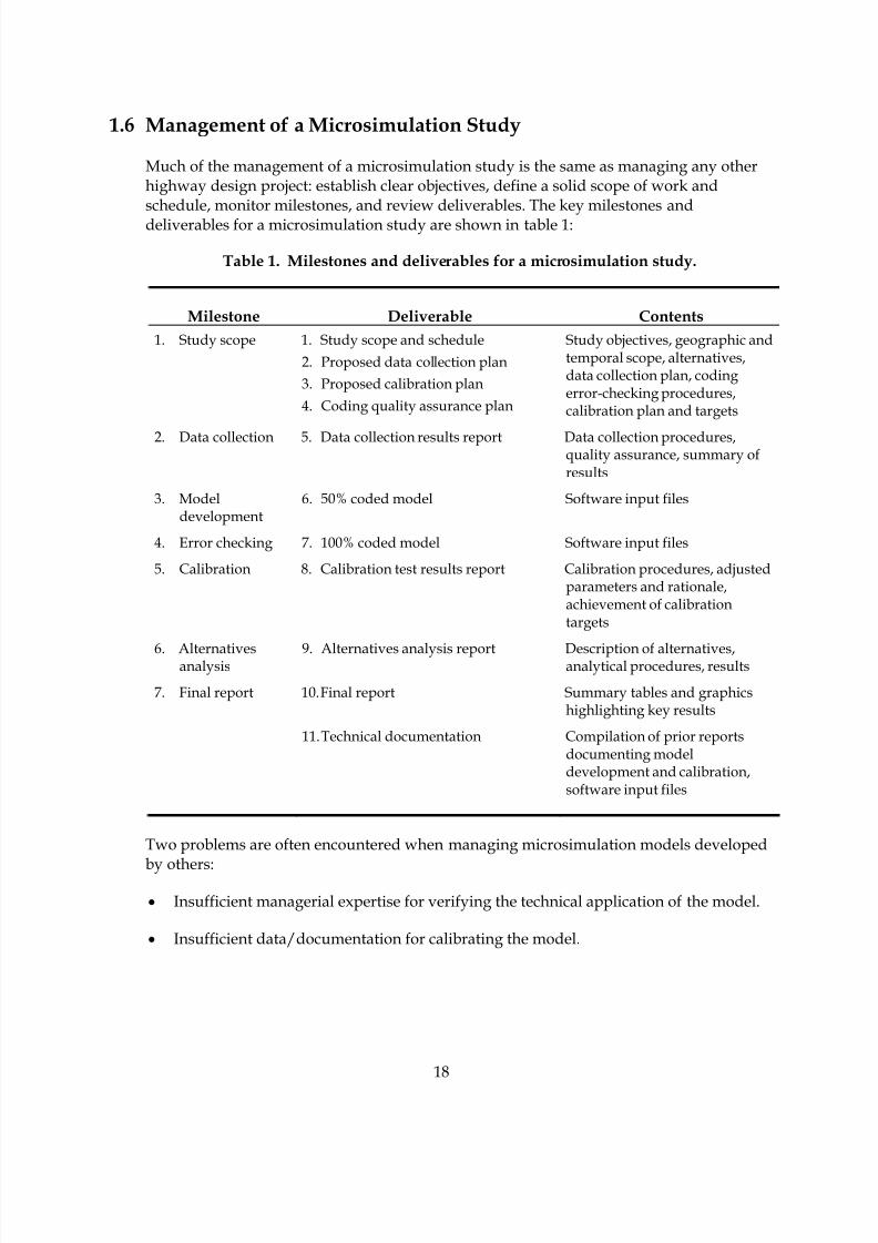
Much of the management of a microsimulation study is the same as managing any otherhighway design project: establish clear objectives, define a solid scope of work andschedule, monitor milestones, and review deliverables. The key milestones anddeliverables for a microsimulation study are shown in table 1:
Table 1. Milestones and deliverables for a microsimulation study.
Milestone Deliverable Contents
1. Study scope 1. Study scope and schedule
2. Proposed data collection plan
3. Proposed calibration plan
4. Coding quality assurance plan
Study objectives, geographic andtemporal scope, alternatives,data collection plan, codingerror-checking procedures,calibration plan and targets
2. Data collection 5. Data collection results report Data collection procedures,quality assurance, summary ofresults
3. Modeldevelopment
6. 50% coded model Software input files
4. Error checking 7. 100% coded model Software input files
5. Calibration 8. Calibration test results report Calibration procedures, adjustedparameters and rationale,achievement of calibrationtargets
6. Alternativesanalysis 9. Alternatives analysis report Description of alternatives,analytical procedures, results
7. Final report 10. Final report Summary tables and graphicshighlighting key results
11. Technical documentation Compilation of prior reportsdocumenting modeldevelopment and calibration,software input files
Two problems are often encountered when managing microsimulation models developed
by others:
• Insufficient managerial expertise for verifying the technical application of the model.
• Insufficient data/documentation for calibrating the model.
8/8/2019 Vol3 Guidelines
http://slidepdf.com/reader/full/vol3-guidelines 29/146
19
The study manager may choose to bring more expertise to the review of the model byforming a technical advisory panel. Furthermore, use of a panel may support a project ofregional importance and detail, or address stakeholder interests regarding the acceptanceof new technology. The panel may be drawn from experts at other public agencies,consultants, or from a nearby university. The experts should have had prior experience
developing simulation models with the specific software being used for the particularmodel.
The manager (and the technical advisory panel) must have access to the input files and thesoftware for the microsimulation model. There are several hundred parameters involvedin the development and calibration of a simulation model. Consequently, it is impossibleto assess the technical validity of a model based solely on its printed output and visualanimation of the results. The manager must have access to the model input files so that heor she can assess the veracity of the model by reviewing the parameter values that go intothe model and looking at its output.
Finally, good documentation of the model calibration process and the rationale forparameter adjustments is required so that the technical validity of the calibrated modelcan be assessed. A standardized format for the calibration report can expedite the reviewprocess.
1.7 Example Problem: Study Scope and Purpose
The example problem is a study of the impact of freeway ramp metering on freeway andsurface-street operations. Ramp metering will be operational during the afternoon peakperiod on the eastbound on-ramps at two interchanges.7
Study Objectives: To quantify the traffic operation benefits and the impact of theproposed afternoon peak-period ramp metering project on both the freeway and nearbysurface streets. The information will be provided to technical people at both the Statedepartment of transportation (DOT) and the city public works department.
Study Breadth (Geographic): The ramp metering project is expected to impact freewayand surface-street operations several miles upstream and downstream of the two meteredon-ramps. However, the most significant impact is expected in the immediate vicinity ofthe meters (the two interchanges, the closest parallel arterial streets, and the cross-connector streets between the interchanges and the parallel arterial). If the negative impact
7 This example problem is part of a larger project involving metering of several miles of freeway.The study area in the example problem was selected to illustrate the concepts and procedures inthe microsimulation guide.

8/8/2019 Vol3 Guidelines
http://slidepdf.com/reader/full/vol3-guidelines 30/146
20
of the ramp meters is acceptable in the immediate vicinity of the project, then the impactfarther away should be of a lower magnitude and, therefore, also acceptable.8
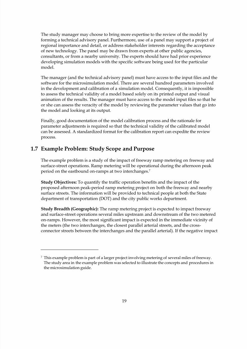
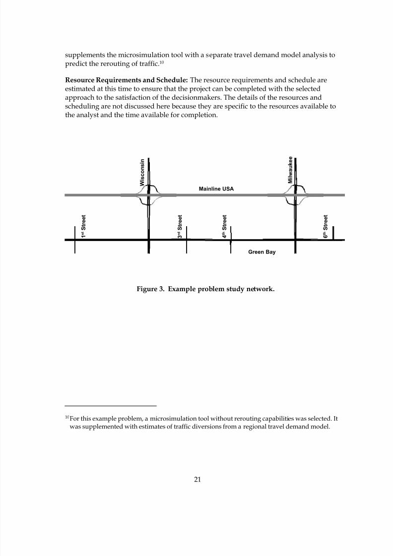
There is no parallel arterial street north of the freeway, so only the parallel arterial on thesouth side needs to be studied. Figure 3 illustrates the selected study area. There are six
signalized intersections along the study section of the Green Bay Avenue parallel arterial.The signals are operating on a common 90-second (s) cycle length. The signals at the ramp junctions on Wisconsin and Milwaukee Avenues also operate on a 90-s cycle length.
The freeway and the adjacent arterial are currently not congested during the afternoonpeak period and, consequently, the study area only needs to be enlarged to encompassprojected future congestion. The freeway and the arterial are modeled 1.6 km (1 mi) eastand west of the two interchanges to include possible future congestion under the “no meter” and “meter” alternatives.
Study Breadth (Temporal): Since there is no existing congestion on the freeway and
surface streets, and the ramp metering will occur only in the afternoon peak hour, theafternoon peak hour is selected as the temporal boundaries for the analysis.9
Analytical Approach: There are concerns that: (1) freeway traffic may be diverted to citystreets causing unacceptable congestion, and (2) traffic at metered on-ramps may backupand adversely impact surface-street operations. A regional travel demand model wouldprobably not be adequate to estimate traffic diversion caused by a regional ramp meteringsystem because it could not model site- and time-specific traffic queues accurately andwould not be able to predict the impact of the meters on surface-street operations. HCMmethods could estimate the capacity impact of ramp metering; however, because thesemethods are not well adapted to estimating the impact of downstream congestion onupstream traffic operations, they are not sufficient by themselves for the analysis of the
impact of ramp meters on surface-street operations. Microsimulation would probablyassist the analyst in predicting traffic diversions between the freeway and surface streets,and would be the appropriate analytical tool for this problem.
Analytical Tool: The analyst selects a microsimulation tool that either incorporates aprocedure for the rerouting of freeway traffic in response to ramp metering, or the analyst
8 Of course, if the analyst does not believe this to be true, then the study area should be expandedaccordingly.
9 If existing or future congestion on either the freeway or arterial was expected to last more than1 h, then the analysis period would be extended to encompass all of the existing and futurecongestion in the study area.
8/8/2019 Vol3 Guidelines
http://slidepdf.com/reader/full/vol3-guidelines 31/146
21
supplements the microsimulation tool with a separate travel demand model analysis topredict the rerouting of traffic.10
Resource Requirements and Schedule: The resource requirements and schedule areestimated at this time to ensure that the project can be completed with the selected
approach to the satisfaction of the decisionmakers. The details of the resources andscheduling are not discussed here because they are specific to the resources available tothe analyst and the time available for completion.
Green Bay
Mainline USA W i s c o n s i n
M i l w a u k e e
1 s t S t r e e t
3 r d S t r e e t
4 t h S t r e e t
6 t h S t r e e t
Figure 3. Example problem study network.
10For this example problem, a microsimulation tool without rerouting capabilities was selected. Itwas supplemented with estimates of traffic diversions from a regional travel demand model.

8/8/2019 Vol3 Guidelines
http://slidepdf.com/reader/full/vol3-guidelines 32/146
8/8/2019 Vol3 Guidelines
http://slidepdf.com/reader/full/vol3-guidelines 33/146
23
No
Data Collection
- Traffic volumes- Base maps/inventory- Field observations
2
1
Project Scope
- Define project purpose- Identify influence areas- Select approach
- Select model
- Estimate staff time
See Chapter 1
See Chapter 2
See Chapter 3
See Chapter 4
Work prior to
actual modeling
Initial
modeling
Yes
Calibrated Model
See Chapter 5
Calibration
See Chapter 6
See Chapter 7
Model
Application
Base Model Development
-Input data- Develop quality assurance
3
Error Checking
- Review Inputs- Review Animation
4
Compare Model
MOEs to Field Data
- Volumes & speeds match?- Congestion in right places?
5
Alternatives Analysis
- Forecast Demand-Base Case- Project Alternatives
6
Final Report
- Key Results
- Technical Documentation
7
Working Model
Before Calibration
Acceptable
Match
Adjust Model Parameters
-Modi fy Global Parameters
-Modify Link Parameters-Modi fy Route Choice Parameters
2.0 Data Collection/Preparation
This chapter provides guidance on the identification,
collection, and preparation of the data sets needed todevelop a microsimulation model for a specificproject analysis, and the data needed to evaluate thecalibration and fidelity of the model to real-worldconditions present in the project analysis study area.There are agency-specific techniques and guidancedocuments that focus on data collection, whichshould be used to support project-specific needs.
A selection of general guides on the collection oftraffic data includes:
Introduction to Traffic Engineering: A Manual for DataCollection and Analysis, T.R. Currin, Brooks/Cole, 2001, 140 pp., ISBN No. 0-534378-67-6.
Manual of Transportation Engineering Studies, H. Douglas Robertson, Joseph E. Hummer,and Donna C. Nelson, Institute of Transportation Engineers, Washington, DC, 1994, ISBNNo. 0-13-097569-9.
Highway Capacity Manual 2000, TRB, 2000, 1200 pp., ISBN No. 0-309067-46-4.
These sources should be consulted regarding appropriate data collection methods (theyare not all-inclusive on the subject of data collection). The discussion in this chapter
focuses on data requirements, potential data sources, and the proper preparation of datafor use in microsimulation analysis.
If the amount of available data does not adequately support the project objectives andscope identified in task 1, then the project team should return to task 1 and redefine theobjectives and scope so that they will be sufficiently supported by the available data.
2.1 Required Data
The precise input data required by a microsimulation model will vary by software and thespecific modeling application as defined by the study objectives and scope. Most
microsimulation analytical studies will require the following types of input data:11
11The forecasting of future demands (turning volumes, O-D table) is discussed later under theAlternatives Analysis task.
8/8/2019 Vol3 Guidelines
http://slidepdf.com/reader/full/vol3-guidelines 34/146
24
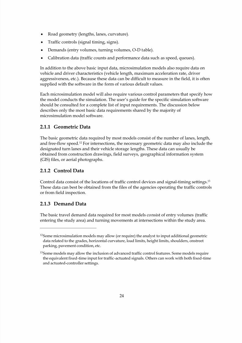
• Road geometry (lengths, lanes, curvature).
• Traffic controls (signal timing, signs).
• Demands (entry volumes, turning volumes, O-D table).
• Calibration data (traffic counts and performance data such as speed, queues).
In addition to the above basic input data, microsimulation models also require data onvehicle and driver characteristics (vehicle length, maximum acceleration rate, driveraggressiveness, etc.). Because these data can be difficult to measure in the field, it is oftensupplied with the software in the form of various default values.
Each microsimulation model will also require various control parameters that specify howthe model conducts the simulation. The user’s guide for the specific simulation softwareshould be consulted for a complete list of input requirements. The discussion belowdescribes only the most basic data requirements shared by the majority ofmicrosimulation model software.
2.1.1 Geometric Data
The basic geometric data required by most models consist of the number of lanes, length,and free-flow speed.12 For intersections, the necessary geometric data may also include thedesignated turn lanes and their vehicle storage lengths. These data can usually beobtained from construction drawings, field surveys, geographical information system(GIS) files, or aerial photographs.
2.1.2 Control Data
Control data consist of the locations of traffic control devices and signal-timing settings.13 These data can best be obtained from the files of the agencies operating the traffic controlsor from field inspection.
2.1.3 Demand Data
The basic travel demand data required for most models consist of entry volumes (trafficentering the study area) and turning movements at intersections within the study area.
12Some microsimulation models may allow (or require) the analyst to input additional geometric
data related to the grades, horizontal curvature, load limits, height limits, shoulders, onstreetparking, pavement condition, etc.
13Some models may allow the inclusion of advanced traffic control features. Some models requirethe equivalent fixed-time input for traffic-actuated signals. Others can work with both fixed-timeand actuated-controller settings.
8/8/2019 Vol3 Guidelines
http://slidepdf.com/reader/full/vol3-guidelines 35/146
25
Some models require one or more vehicular O-D tables, which enable the modeling ofroute diversions. Procedures exist in many demand modeling software and somemicrosimulation software for estimating O-D tables from traffic counts.
Count Locations and Duration
Traffic counts should be conducted at key locations within the microsimulation modelstudy area for the duration of the proposed simulation analytical period. The countsshould ideally be aggregated to no longer than 15-minute (min) time periods; however,alternative aggregations can be used if dictated by circumstances.14
If congestion is present at a count location (or upstream of it), care should be taken toensure that the count measures demand and not capacity. The count period should ideallystart before the onset of congestion and end after the dissipation of all congestion toensure that all queued demand is eventually included in the count.
The counts should be conducted simultaneously if resources permit so that all countinformation is consistent with a single simulation period. Often, resources do not permitthis for the larger simulation areas, so the analyst must establish one or more controlstations where a continuous count is maintained over the length of the data collectionperiod. The analyst then uses the control station counts to adjust the counts collected overseveral days into a single consistent set of counts representative of a single typical daywithin the study area.
Estimating Origin-Destination (O-D) Trip Tables
For some simulation software, the counts must be converted into an estimate of existingO-D trip patterns. Other software programs can work with either turning-movement
counts or an O-D table. An O-D table is required if it is desirable to model route choiceshifts within the microsimulation model.
Local metropolitan planning organization (MPO) travel demand models can provide O-Ddata; however, these data sets are generally limited to the nearest decennial census yearand the zone system is usually too macroscopic for microsimulation. The analyst mustusually estimate the existing O-D table from the MPO O-D data in combination with otherdata sources, such as traffic counts. This process will probably require consideration ofO-D pattern changes resulting from the time of day, especially for simulations that coveran extended period of time throughout the day.
A license plate matching survey is the most accurate method for measuring existing O-Ddata. The analyst establishes checkpoints within and on the periphery of the study area
14Project constraints, traffic counter limitations, or other considerations (such as a long simulationperiod) may require that counts be aggregated to longer or shorter periods.
8/8/2019 Vol3 Guidelines
http://slidepdf.com/reader/full/vol3-guidelines 36/146
26
and notes the license plate numbers of all vehicles passing by each checkpoint. A matchingprogram is then used to determine how many vehicles traveled between each pair ofcheckpoints. However, license plate surveys can be quite expensive. For this reason, theestimation of the O-D table from traffic counts is often selected.15
Vehicle Characteristics
The vehicle characteristics typically include vehicle mix, vehicle dimensions, and vehicleperformance characteristics (maximum acceleration, etc.).16
Vehicle Mix: The vehicle mix is defined by the analyst, often in terms of the percentage oftotal vehicles generated in the O-D process. Typical vehicle types in the vehicle mix mightbe passenger cars, single-unit trucks, semi-trailer trucks, and buses.
Default percentages are usually included in most software programs; however, the vehiclemix is highly localized and national default values will rarely be valid for specific
locations. For example, the percentage of trucks in the vehicle mix can vary from a low of2 percent on urban streets during rush hour to a high of 40 percent of daily weekdaytraffic on an intercity interstate freeway.
It is recommended that the analyst obtain one or more vehicle classification studies for thestudy area for the time period being analyzed. Vehicle classification studies can often beobtained from nearby truck weigh station locations.
Vehicle Dimensions and Performance: The analyst should attempt to obtain the vehiclefleet data (vehicle mix, dimensions, and performance) from the local State DOT or airquality management agency. National data can be obtained from the Motor andEquipment Manufacturers Association (MEMA), various car manufacturers, FHWA, and
the U.S. Environmental Protection Agency (EPA). In the absence of data from thesesources, the analyst may use the defaults shown in table 2.
15There are many references in the literature on the estimation of O-D volumes from traffic counts.Appendix A, chapter 29, HCM 2000 provides a couple of simple O-D estimation algorithms. Most
travel demand software and some microsimulation software have O-D estimation modulesavailable.
16The software-supplied default vehicle mix, dimensions, and performance characteristics shouldbe reviewed to ensure that they are representative of local vehicle fleet data, especially forsimulation software developed outside the United States.
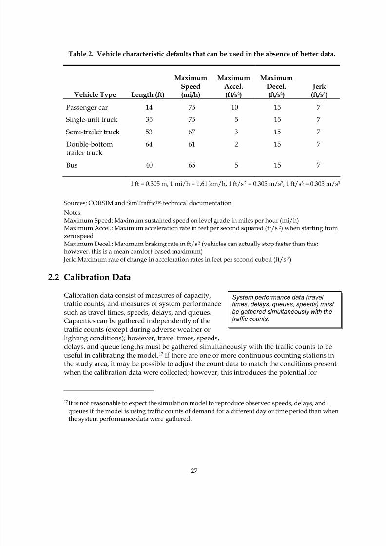
8/8/2019 Vol3 Guidelines
http://slidepdf.com/reader/full/vol3-guidelines 37/146
27
Table 2. Vehicle characteristic defaults that can be used in the absence of better data.
Vehicle Type Length (ft)
MaximumSpeed
(mi/h)
MaximumAccel.
(ft/s2)
MaximumDecel.
(ft/s2)
Jerk
(ft/s3)
Passenger car 14 75 10 15 7
Single-unit truck 35 75 5 15 7
Semi-trailer truck 53 67 3 15 7
Double-bottomtrailer truck
64 61 2 15 7
Bus 40 65 5 15 7
1 ft = 0.305 m, 1 mi/h = 1.61 km/h, 1 ft/s2 = 0.305 m/s2, 1 ft/s3 = 0.305 m/s3
Sources: CORSIM and SimTraffic™ technical documentation
Notes:Maximum Speed: Maximum sustained speed on level grade in miles per hour (mi/h)Maximum Accel.: Maximum acceleration rate in feet per second squared (ft/s2) when starting fromzero speedMaximum Decel.: Maximum braking rate in ft/s2 (vehicles can actually stop faster than this;however, this is a mean comfort-based maximum)
Jerk: Maximum rate of change in acceleration rates in feet per second cubed (ft/s3)
2.2 Calibration Data
Calibration data consist of measures of capacity,traffic counts, and measures of system performancesuch as travel times, speeds, delays, and queues.Capacities can be gathered independently of thetraffic counts (except during adverse weather orlighting conditions); however, travel times, speeds,delays, and queue lengths must be gathered simultaneously with the traffic counts to beuseful in calibrating the model.17 If there are one or more continuous counting stations inthe study area, it may be possible to adjust the count data to match the conditions presentwhen the calibration data were collected; however, this introduces the potential for
17It is not reasonable to expect the simulation model to reproduce observed speeds, delays, andqueues if the model is using traffic counts of demand for a different day or time period than whenthe system performance data were gathered.
System performance data (travel times, delays, queues, speeds) must be gathered simultaneously with thetraffic counts.
8/8/2019 Vol3 Guidelines
http://slidepdf.com/reader/full/vol3-guidelines 38/146
28
additional error in the calibration data and weakens the strength of the conclusions thatcan be drawn from the model calibration task.
Finally, the analyst should verify that the documented signal-timing plans coincide withthose operating in the field. This will confirm any modifications resulting from a signal
retiming program.
2.2.1 Field Inspection
It is extremely valuable to observe existing operations in the field during the time periodbeing simulated. Simple visual inspection can identify behavior not apparent in countsand floating car runs. Video images may be useful; however, they may not focus on theupstream conditions causing the observed behavior, which is why a field visit duringpeak conditions is always important. A field inspection is also valuable for aiding themodeler in identifying potential errors in data collection.
2.2.2 Travel Time Data
The best source of point-to-point travel time data is “floating car runs.” In this method,one or more vehicles are driven the length of the facility several times during theanalytical period and the mean travel time is computed. The number of vehicle runsrequired to establish a mean travel time within a 95-percent confidence level depends onthe variability of the travel times measured in the field. Free-flow conditions may requireas few as three runs to establish a reliable mean travel time. Congested conditions mayrequire 10 or more runs.
The minimum number of floating car runs needed to determine the mean travel time
within a desired 95-percent confidence interval depends on the width of the interval thatis acceptable to the analyst. If the analyst wishes to calibrate the model to a very tighttolerance, then a very small interval will be desirable and a large number of floating carruns will be required. The analyst might aim for a confidence interval of ± 10 percent ofthe mean travel time. Thus, if the mean travel time were 10 min, the target 95-percentconfidence interval would be 2 min. The number of required floating car runs is obtainedfrom equation 1:
2
1,025.02
∗= −
R
st N N (1)
where:
R = 95-percent confidence interval for the true mean
t0.025,N-1 = Student’s t-statistic for two-sided error of 2.5 percent (totals 5 percent) with N-1degrees of freedom (for four runs, t = 3.2; for six runs, t = 2.6; for 10 runs, t = 2.3)
8/8/2019 Vol3 Guidelines
http://slidepdf.com/reader/full/vol3-guidelines 39/146
29
(Note: There is one less degree of freedom than car runs when looking up the appropriatevalue of t in the statistical tables.)
s = standard deviation of the floating car runs
N = number of required floating car runs
For example, if the floating car runs showed a standard deviation of 1.0 min, a minimumof seven floating car runs would be required to achieve a target 95-percent confidenceinterval of 2.0 min (± 1.0 min) for the mean travel time.
The analyst is advised that the standard deviation is unknown prior to runs beingconducted. In addition, the standard deviation is typically higher under more congestedconditions.
2.2.3 Point Speed Data
Traffic management centers (TMCs) are a good source of simultaneous speed and flowdata for urban freeways. Loop detectors, though, may be subject to failure, so the datamust be reviewed carefully to avoid extraneous data points. Loop detectors are typicallyspaced 0.5 to 0.8 km (0.3 to 0.5 mi) apart and their detection range is limited to 3.7 meters(m) (12 feet (ft)). Under congested conditions, much can happen between detectors, so themean speeds produced by the loop detectors cannot be relied on to give system traveltimes under congested conditions.
The loop-measured free-flow speeds may be reliable for computing facility travel timesunder uncongested conditions; however, care should be taken when using these data.Many locations have only single-loop detectors in each lane, so the free-flow speed must
be estimated from an assumed mean vehicle length. The assumed mean vehicle lengthmay be automatically calibrated by the TMC; however, this calibration requires somemethod of identifying which data points represent free-flow speed, which data points donot, and which ones are aberrations. The decision process involves some uncertainty. Inaddition, the mix of trucks and cars in the traffic stream varies by time of day, thus thesame mean vehicle length cannot be used throughout the day. Overall, loop-estimated/-measured free-flow speeds should be treated with a certain amount of caution.They are precise enough for identifying the onset of congestion; however, they may not bean accurate measure of speed.
2.2.4 Capacity and Saturation Flow Data
Capacity and saturation flow data are particularly valuable calibration data since theydetermine when the system goes from uncongested to congested conditions:
• Capacity can be measured in the field on any street segment immediately downstreamof a queue of vehicles. The queue should ideally last for a full hour; however,
8/8/2019 Vol3 Guidelines
http://slidepdf.com/reader/full/vol3-guidelines 40/146
30
reasonable estimates of capacity can be obtained if the queue lasts only 0.5 hour (h).The analyst would simply count the vehicles passing a point on the downstreamsegment for 1 h (or for a lesser time period if the queue does not persist for a full hour)to obtain the segment capacity.
• Saturation flow rate is defined as “the equivalent hourly rate at which previouslyqueued vehicles can traverse an intersection approach under prevailing conditions,assuming that the green signal is available at all times and no lost times areexperienced, in vehicles per hour or vehicles per hour per lane.”18 The saturation flowrate should be measured (using procedures specified in the HCM) at all signalizedintersections that are operating at or more than 90 percent of their existing capacity.At these locations, the estimation of saturation flow and, therefore, capacity willcritically affect the predicted operation of the signal. Thus, it is cost-effective toaccurately measure the saturation flow and, therefore, capacity at these intersections.
2.2.5 Delay and Queue Data
Delay can be computed from floating car runs or from delay studies at individualintersections. Floating car runs can provide satisfactory estimates of delay along thefreeway mainline; however, they are usually too expensive to make all of the necessaryadditional runs to measure all of the ramp delays. Floating cars are somewhat biasedestimators of intersection delay on surface streets since they reflect only those vehiclestraveling a particular path through the network. For an arterial street with coordinatedsignal timing, the floating cars running the length of the arterial will measure delay onlyfor the through movement with favorable progression. Other vehicles on the arterial willexperience much greater delays. This problem can be overcome by running the floatingcars on different paths; however, the cost may be prohibitive.
Comprehensive measures of intersection delay can be obtained from surveys of stoppeddelay on the approaches to an intersection (see the HCM for the procedure). The numberof stopped cars on an approach is counted at regular intervals, such as every 30 s. Thenumber of stopped cars multiplied by the counting interval (30 s) gives the total stoppeddelay. Dividing the total stopped delay by the total number of vehicles that crossed thestop line (a separate count) during the survey period gives the mean stopped delay pervehicle. The stopped delay can be converted to the control delay using the procedure inappendix A of chapter 16 in the HCM.
2.3 Data Preparation/Quality Assurance
Data preparation consists of review, error checking, and the reduction of the datacollected in the field. Data reduction is already well covered in other manuals on data
18HCM 2000.
8/8/2019 Vol3 Guidelines
http://slidepdf.com/reader/full/vol3-guidelines 41/146
31
collection. This section consequently focuses on review and error checking of the data. Thefollowing checks of the data should be made during the data preparation step:
• Geometric and control data should be reviewed for apparent violations of designstandards and/or traffic engineering practices. Sudden breaks in geometric continuity
(such as a short block of a two-lane street sandwiched in between long stretches of afour-lane street) may also be worth checking with people who are knowledgeableabout local conditions. Breaks in continuity and violations of design standards may beindicative of data collection errors.
• Internal consistency of counts should be reviewed. Upstream counts should becompared to downstream counts. Unexplained large jumps or drops in the countsshould be reconciled.19
• Floating car run results should be reviewed for realistic segment speeds.
• Counts of capacity and saturation flow should be compared to the HCM estimates forthese values. Large differences between field measurements and the HCM warrant
double-checking the field measurements and the HCM computations.20
2.4 Reconciliation of Traffic Counts
Inevitably, there will be traffic counts at two or more nearby adjacent locations that do notmatch. This may be a result of counting errors, counting on different days (countstypically vary by 10 percent or more on a daily basis), major traffic sources (or sinks)between the two locations, or queuing between the two locations. In the case of a freeway,a discrepancy between the total traffic entering the freeway and the total exiting it may be
caused by storage or discharge of some of the vehicles in growing or shrinking queues onthe freeway.
The analyst must review the counts and determine (based on local knowledge and fieldobservations) the probable causes of the discrepancies. Counting errors and counts made
19There is no guidance on precisely what constitutes a “large” difference in counts. The analystmight consider investigating any differences of greater than 10 percent between upstream anddownstream counts for locations where no known traffic sources or sinks (such as driveways)exist between the count locations. Larger differences are acceptable where driveways and parking
lots could potentially explain the count differences.
20There is no guidance on precisely how large differences can be between the HCM and fieldmeasurements before the field measurements may be suspect. The analyst might consider 25-percent differences to be within the normal range of accuracy of the HCM and take a second lookat the calculations and field measurements if the differences are greater than that.
8/8/2019 Vol3 Guidelines
http://slidepdf.com/reader/full/vol3-guidelines 42/146
32
on different days are treated differently than counting differences caused by midblocksources/sinks or midblock queuing.
Discrepancies in the counts resulting from counting errors or counts made on differentdays must be reconciled before proceeding to the model development task. Inconsistent
counts make error checking and model calibration much more difficult. Differing countsfor the same location should be normalized or averaged assuming that they arereasonable. This is especially true for entry volumes into the model network. Intersectionturning volumes should be expressed as percentages based on an average of the countsobserved for that location. This will greatly assist with calibrating the model later.
Differences in counts caused by midblock sources (such as a parking lot) need not bereconciled; however, they must be dealt with by coding midblock sources and sinks in thesimulation model during the model development task.
Differences in entering and exiting counts that are caused by queuing in between the two
count locations suggest that the analyst should extend the count period to ensure that alldemand is included in both counts.
Accurate vehicle classification counts and accurate travel speeds can also affect the trafficvolumes. Trucks and other large vehicles and inaccurate speeds can skew the volumecounts.
2.5 Example Problem: Data Collection and Preparation
The same ramp metering example problem discussed in chapter 1.0 is continued here.Now the task is to identify, gather, and prepare the data for the study area and theafternoon peak-hour analytical period.
Road Geometry: Aerial photographs, construction drawings, and field inspections areused to obtain the lengths and the number of lanes for each section of the freeway, ramps,and surface streets. Turn lanes and pocket lengths are determined for each intersection.Transition lengths for lane drops and additions are determined. Lane widths aremeasured if they are not standard widths. Horizontal curvature and curb return radii aredetermined if the selected software tool is sensitive to these features of the road andfreeway design. Free-flow speeds are estimated based on the posted speed limits for thefreeway and the surface streets.
Traffic Controls: Existing signal settings were obtained from the agencies’ records and
verified in the field. The controllers at the interchange ramp terminals are all fixed-time,having a cycle length of 90 s. The signals along Green Bay Avenue are traffic-actuated.
Demands: Field measurements of traffic volumes on the freeway mainline and ramps, andturning-movement counts at each intersection were conducted for a 2-h period during the

8/8/2019 Vol3 Guidelines
http://slidepdf.com/reader/full/vol3-guidelines 43/146
33
afternoon peak period (4:00 to 6:00 p.m.). The peak hour was determined to be between5:00 and 6:00 p.m., and the highest 15-min volumes occurred between 5:30 and 5:45 p.m.
Vehicle Characteristics: The default vehicle mix and characteristics provided with themicrosimulation software were used in this analysis.21
Calibration Data: The model will be calibrated against estimates of capacity and trafficcounts, and the system performance will be assessed against travel time data.
Saturation flows for protected movements at traffic signals were estimated using the HCM2000 methodology and verified through field observations at a few approaches with longqueues.22
Capacity values for basic freeway segments were estimated using the HCM 2000procedures.23
The traffic count data have already been discussed.
The system performance calibration data were obtained at the same time as the trafficcounts, which consisted of travel times obtained from floating car runs, delays at trafficsignals, and speeds on the freeway.
Data Preparation: The input data were reviewed by the analyst for consistency andaccuracy prior to data entry. The turning, ramp, and freeway mainline counts werereconciled by the analyst to produce a set of consistent counts for the entire study area.After completion of the reconciliation, all volumes discharged from upstream locations areequal to the volumes arriving at the downstream location. Based on local knowledge ofthe area, the analyst determined that midblock sources were not required for the surface
streets in the study area.
21The selected software had been developed with defaults appropriate to the United States, and thiswas considered to be sufficiently accurate for this planning study of ramp metering.
22The HCM was used to estimate surface-street saturation flow rates because none of theintersections were currently operating nor were they expected to operate within 90 percent of
their capacity. Thus, an estimate is sufficiently accurate. Field measurements were not required.
23The HCM was used to estimate freeway capacity because there is no freeway congestion underexisting conditions that would enable field measurement of capacities. Another method would beto observe capacities on a similar type of facility in the area that operated under congestedconditions. This method may be preferred if a comparable facility can be found.

8/8/2019 Vol3 Guidelines
http://slidepdf.com/reader/full/vol3-guidelines 44/146
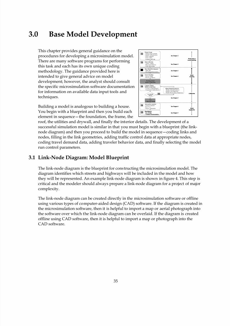
8/8/2019 Vol3 Guidelines
http://slidepdf.com/reader/full/vol3-guidelines 45/146
35
No
Data Collection
- Traffic volumes- Base maps/inventory- Field observations
2
1
Project Scope
- Define project purpose- Identify influence areas- Select approach- Select model- Estimate staff time
See Chapter 1
See Chapter 2
See Chapter 3
See Chapter 4
Work prior to
actual modeling
Initial
modeling
Yes
Calibrated Model
See Chapter 5
Calibration
See Chapter 6
See Chapter 7
Model
Application
Base Model Development
- Input data- Develop qualityassurance
3
Error Checking
- Review Inputs- Review Animation
4
Compare ModelMOEs to Field Data
- Volumes & speedsmatch?- Congestion in right places?
5
Alternatives Analysis
- Forecast Demand-Base Case- Project Alternatives
6
Final Report
- Key Results
- Technical Documentation
7
Working Model
Before Calibration
Acceptable
Match
Adjust Model Parameters
- Modify Global Parameters- Modify Link Parameters- Modify Route Choice Parameters
3.0 Base Model Development
This chapter provides general guidance on the
procedures for developing a microsimulation model.There are many software programs for performingthis task and each has its own unique codingmethodology. The guidance provided here isintended to give general advice on modeldevelopment; however, the analyst should consultthe specific microsimulation software documentationfor information on available data input tools andtechniques.
Building a model is analogous to building a house.You begin with a blueprint and then you build eachelement in sequence—the foundation, the frame, theroof, the utilities and drywall, and finally the interior details. The development of asuccessful simulation model is similar in that you must begin with a blueprint (the link-node diagram) and then you proceed to build the model in sequence—coding links andnodes, filling in the link geometries, adding traffic control data at appropriate nodes,coding travel demand data, adding traveler behavior data, and finally selecting the modelrun control parameters.
3.1 Link-Node Diagram: Model Blueprint
The link-node diagram is the blueprint for constructing the microsimulation model. Thediagram identifies which streets and highways will be included in the model and howthey will be represented. An example link-node diagram is shown in figure 4. This step iscritical and the modeler should always prepare a link-node diagram for a project of majorcomplexity.
The link-node diagram can be created directly in the microsimulation software or offlineusing various types of computer-aided design (CAD) software. If the diagram is created inthe microsimulation software, then it is helpful to import a map or aerial photograph intothe software over which the link-node diagram can be overlaid. If the diagram is createdoffline using CAD software, then it is helpful to import a map or photograph into theCAD software.

8/8/2019 Vol3 Guidelines
http://slidepdf.com/reader/full/vol3-guidelines 46/146
36
Figure 4. Example of link-node diagram.
Nodes are the intersection of two or more links. Nodes are usually placed in the modelusing x-y coordinates and they can be at a place that represents an intersection or alocation where there is a change in the link geometry. Some simulation software may alsowarrant consideration of a z coordinate. The node locations can be obtained from aerialphotographs, maps, or physical measurements.
FreewayInterchange
Link-NodeDiagram

8/8/2019 Vol3 Guidelines
http://slidepdf.com/reader/full/vol3-guidelines 47/146
37
Links are one-directional segments of surface streets or freeways.24 Links represent thelength of the segment and usually contain data on the geometric characteristics of the roador highway between the nodes. Ideally, a link represents a roadway segment withuniform geometry and traffic operation conditions.25
The analyst should consider establishing a node-numbering scheme to facilitate errorchecking and the aggregation of performance statistics for groups of links related to aspecific facility or facility type (see table 3 for an example of a node-numbering schemedesigned to enable the rapid determination of the facility type in text output). Much of theoutput produced by microsimulation software is text, with the results identified by thenode numbers at the beginning and end points of each link. A node-numberingconvention can greatly facilitate the search for results in the massive text files commonlyproduced by simulation software.26
If the link-node diagram was created offline (using some other software besides themicrosimulation software), then the information in the diagram needs to be entered (or
imported) into the microsimulation software. The x-y coordinates and identificationnumbers of the nodes (plus any feature points needed to represent link curvature) areentered. The nodes are then connected together to develop the link-node framework forthe model.
24Some software programs do not always use a link-node scheme, while others allow the analyst tocode both directions of travel with a single link. The two-way links coded by the user are thenrepresented internally (inside the software) as two one-way links.
25The analyst may find it desirable to split links for performance reporting purposes. For example,it may be desirable to report density separately for the 460 m (1500-ft) influence area on thefreeway near a ramp merge or diverge. However, the analyst should be cautious about thepotential impact of split links on the ability of the software to accurately simulate vehiclebehavior.
26Some software programs provide analytical modules that assist the analyst in displaying andaggregating the results for specific groups of links. This feature reduces the necessity of adoptinga node-numbering convention; however, a numbering convention can still result in a significantlabor savings when reviewing text output or when importing text results into other softwareprograms for analytical purposes.
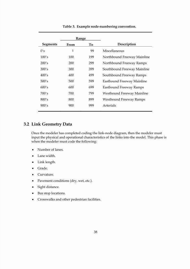
8/8/2019 Vol3 Guidelines
http://slidepdf.com/reader/full/vol3-guidelines 48/146
38
Table 3. Example node-numbering convention.
Range
Segments From To Description
0’s 1 99 Miscellaneous
100’s 100 199 Northbound Freeway Mainline
200’s 200 299 Northbound Freeway Ramps
300’s 300 399 Southbound Freeway Mainline
400’s 400 499 Southbound Freeway Ramps
500’s 500 599 Eastbound Freeway Mainline
600’s 600 699 Eastbound Freeway Ramps
700’s 700 799 Westbound Freeway Mainline800’s 800 899 Westbound Freeway Ramps
900’s 900 999 Arterials
3.2 Link Geometry Data
Once the modeler has completed coding the link-node diagram, then the modeler mustinput the physical and operational characteristics of the links into the model. This phase is
when the modeler must code the following:
• Number of lanes.
• Lane width.
• Link length.
• Grade.
• Curvature.
• Pavement conditions (dry, wet, etc.).
• Sight distance.• Bus stop locations.
• Crosswalks and other pedestrian facilities.
8/8/2019 Vol3 Guidelines
http://slidepdf.com/reader/full/vol3-guidelines 49/146
39
• Bicycle lanes/paths.
• Others.
The specific data to be coded for the links will vary according to the microsimulationsoftware.
3.3 Traffic Control Data at Intersections and Junctions
Most microsimulation uses a time-step simulation to describe traffic operations (which isusually 1 s or less). Vehicles are moved according to car-following logic in response totraffic control devices and in response to other demands. Traffic control devices formicrosimulation models will vary. Listed below are some examples:
• No control.
• Yield signs.
• Stop signs.
• Signals (pretimed, actuated, real-time traffic adaptive).
• Ramp metering.
3.4 Traffic Operations and Management Data for Links
Traffic operations and management data for links consist of the following:
• Warning data (incidents, lane drops, exits, etc.).
• Regulatory data (speed limits, variable speed limits, high-occupancy vehicles (HOVs),high-occupancy toll (HOT), detours, lane channelizations, lane use, etc.).
• Information (guidance) data (dynamic message signs and roadside beacons).
• Surveillance detectors (type and location).
3.5 Traffic Demand Data
Traffic demands are defined as the number of vehicles and the percentage of vehicles ofeach type that wish to traverse the study area during the simulation time period.
Furthermore, it may be necessary to reflect the variation in demand throughout thesimulation time period. In most software programs, the traffic entering into the network isusually defined by some parameter, and traffic leaving the network is usually computedbased on parameters internal to the network (turning movements, etc.). The modeler mustcode the traffic volume by first starting from the external nodes (this is where the traffic isput into the model). Once all of the entering traffic volumes at the external nodes are
8/8/2019 Vol3 Guidelines
http://slidepdf.com/reader/full/vol3-guidelines 50/146
40
coded, the modeler will then go into the model and define the turning movements andany other parameter related to route choice. The key traffic demand data are:
• Entry volumes by vehicle type and turning fractions at all intersections or junctions(random walk simulators).
• O-D/path-specific and vehicle data (path-specific simulators).
• Bus operations (routes and headways/schedules).
• Bicycle and pedestrian demand data.
3.6 Driver Behavior Data
Default values for driver behavior data are usually provided with the microsimulationsoftware. Users may override the default values of any driver behavior parameters if valid
observed data are available (e.g., desired free-flow speed, discharge headway, startup losttime at intersections, etc.). Driver behavior data include:
• Driver’s aggressiveness (for minimum headway in car-following, gap acceptance forlane changing, response to yellow interval).
• Availability of (real-time) information for the driver.
• Driver’s response to information (for pretrip planning and/or en route switching).
3.7 Events/Scenarios Data
Events data include:
• Blockages and incidents.
• Work zones.
• Parking activity in curb lane.
This data is optional and will vary according to the specific application being developedby the analyst.
3.8 Simulation Run Control Data
All simulation software contain run control parameters to enable the modeler tocustomize the software operation for their specific modeling needs. These parameters willvary between software programs. They generally include:
8/8/2019 Vol3 Guidelines
http://slidepdf.com/reader/full/vol3-guidelines 51/146
41
• Length of simulation time.
• Selected MOEs or output (e.g., reports, animation files, or both).
• Resolution of simulation results (e.g., temporal and special resolution).
• Other system parameters to run the model.
3.9 Coding Techniques for Complex Situations
Microsimulation software allows the modeler to develop a model to represent the real-world situation. However, not all possible real-world situations were necessarilycontemplated when the software was originally written. This is when the modeler, with agood understanding of the operation of the software, can “extend” the software tosimulate conditions not originally incorporated into the microsimulation software.However, this should only be attempted after the tools, resources, and skills available arefully appreciated. This is because new tools continue to become available that account for
selected real-world situations.
Provided below are some examples of how basic microsimulation software can be appliedto less standard situations, noting that calibration (discussed in chapter 5.0) must alsoconsider the following situations:
• A curb lane is heavily used for parking, loading, and unloading activities. As a result,this lane may be blocked virtually all of the time. If the simulation software cannotcorrectly replicate the real situation, the modeler may consider removing this lanefrom the link.
• There is a drawbridge in the real-world network; however, the software does not haveexplicit “drawbridge” modeling capability. If boat traffic is very heavy and isequivalent to vehicular traffic, the modeler may consider coding the drawbridge as anintersection with fixed-time signal control. If boat traffic is irregular, the analyst mightconsider coding the drawbridge as a semi-actuated traffic signal-controlledintersection. If boat traffic is rare, then the drawbridge might be coded as a link withevents that result in a 100-percent capacity loss with a certain probability ofoccurrence during the analytical period.
• Traffic regularly backs up on a freeway off-ramp, backing up onto the freeway.However, instead of stopping on the freeway and blocking a lane, the queue forms onthe shoulder of the freeway, keeping the right-hand lane open. If this is the case in the
study area, the modeler may artificially extend the off-ramp length to realisticallymodel the traffic in the field.

8/8/2019 Vol3 Guidelines
http://slidepdf.com/reader/full/vol3-guidelines 52/146
42
3.10 Quality Assurance/Quality Control (QA/QC) Plan
Once the modeler is satisfied that the model is coded, the modeler must then vet themodel for completeness. This could be a QA/QC process. Many of the models input aredeveloped in a format that can be exported to a spreadsheet format. Therefore, themodeler can use this type of tool to aid in vetting the model for completeness andaccuracy. The next chapter on error checking describes quality control tests in more detail.
3.11 Example Problem: Base Model Development
Continuing with the same example problem from the previous chapters, the task is now tocode the base model.
The first step is to code the link-node diagram. How this is best done can be determinedfrom the software user’s guide. Figure 5 shows the link-node diagram for the exampleproblem.
The next steps are to input:
1. Link geometry data.
2. Intersection traffic control data.
3. Traffic operations and management data.
4. Traffic count data.
5. Run control parameters.27
27The software-provided default values for driver behavior (aggressiveness, awareness, etc.) were
used in this example problem. They were considered to be sufficiently accurate for this analysis.
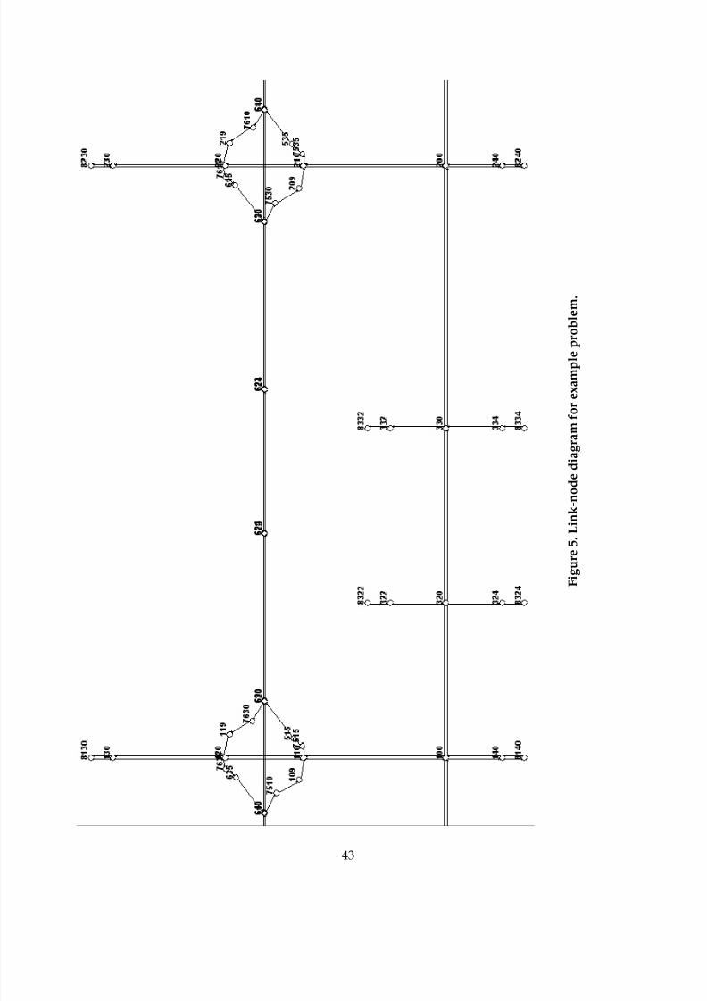
8/8/2019 Vol3 Guidelines
http://slidepdf.com/reader/full/vol3-guidelines 53/146
F i g u r e 5 . L i n k - n o d e d i a g r a m f o r e x a m p l e p r o b l e m .
43

8/8/2019 Vol3 Guidelines
http://slidepdf.com/reader/full/vol3-guidelines 54/146

8/8/2019 Vol3 Guidelines
http://slidepdf.com/reader/full/vol3-guidelines 55/146
45
No
Data Collection
- Traffic volumes- Base maps/inventory- Field observations
2
1
Project Scope
- Define project purpose- Identify influence areas- Select approach
- Select model- Estimate staff time
See Chapter 1
See Chapter 2
See Chapter 3
See Chapter 4
Work prior to
actual modeling
Initial
modeling
Yes
Calibrated Model
See Chapter 5
Calibration
See Chapter 6
See Chapter 7
Model
Application
Base Model Development
- Input data- Develop qualityassurance
3
Error Checking
- Review Inputs- Review Animation
4
Compare Model
MOEs to Field Data
- Volumes & speedsmatch?- Congestion in right places?
5
Alternatives Analysis
- Forecast Demand-Base Case- Project Alternatives
6
Final Report
- Key Results
- Technical Documentation
7
Working Model
Before Calibration
Acceptable
Match
Adjust Model Parameters
- Modify Global Parameters- Modify Link Parameters- Modify Route Choice Parameters
4.0 Error Checking
The error correction step is essential in developing a
working model so that the calibration process does notresult in parameters that are distorted to compensatefor overlooked coding errors. The succeeding steps ofthe calibration process rely on the elimination of allmajor errors in demand and network coding beforecalibration.
Error checking involves various reviews of the codednetwork, coded demands, and default parameters.Error checking proceeds in three basic stages:(1) software error checking, (2) input coding errorchecking, and (3) animation review to spot less obviousinput errors.
4.1 Review Software Errors
The analyst should review the software and user group Web sites to ensure that he or sheis aware of the latest known “bugs” and user workarounds for the software. The analystshould ensure that he or she is using the latest version and “patch” of the software.
4.2 Review Input
A checklist for verifying the accuracy of the coded input data is provided below:
1. Link and node network:
a. Check basic network connectivity (are all connections present?).
b. Check link geometry (lengths, number of lanes, free-flow speed, facility type, etc.).
c. Check intersection controls (control type, control data).
d. Check for prohibited turns, lane closures, and lane restrictions at the intersectionsand on the links.
2. Demand:
a. Check vehicle mix proportions at each entry node/gate/zone.
b. Check identified sources and sinks (zones) for traffic.
c. Verify zone volumes against traffic counts.
d. Check vehicle occupancy distribution (if modeling HOVs).

8/8/2019 Vol3 Guidelines
http://slidepdf.com/reader/full/vol3-guidelines 56/146
46
e. Check turn percentages (if appropriate).
f. Check O-Ds of trips on the network.
3. Traveler behavior and vehicle characteristics:
a. Check and revise, as necessary, the default vehicle types and dimensions.b. Check and revise the default vehicle performance specifications.
The following techniques may be useful to increase the efficiency and effectiveness of theerror-checking process:1
• Overlay the coded network over aerial photographs of the study area to quickly verifythe accuracy of the coded network geometry.
• If working with software that supports three-dimensional modeling, turn on the nodenumbers and look for superimposed numbers. They are an indication of
unintentionally superimposed links and nodes. Two or more nodes placed in the samelocation will look like a single node in a three-dimensional model when viewed in twodimensions. The links may connect to one of the nodes, but not to the other.
• For a large network, a report summarizing the link attributes should be created so thattheir values can be easily reviewed.
• Use color codes to identify links by the specific attribute being checked (e.g., linksmight be color-coded by free-flow speed range). Out-of-range attributes can beidentified quickly if given a particular color. Breaks in continuity can also be spottedquickly (e.g., a series of 56-km/h (35-mi/h) links with one link coded as 40 km/h(25 mi/h)).
4.3 Review Animation
Animation output enables the analyst to see the vehicle behavior that is being modeledand assess the reasonableness of the microsimulation model itself. Running the simulationmodel and reviewing the animation, even with artificial demands, can be useful toidentify input coding errors. The analyst inputs a very low level of demand and thenfollows individual vehicles through the network. Aberrant vehicle behavior (such asunexpected braking or stops) is a quick indicator of possible coding errors.
A two-stage process can be followed in reviewing the animation output:
1. Run the animation at an extremely low demand level (so low that there is nocongestion). The analyst should then trace single vehicles through the network andsee where they unexpectedly slow down. These will usually be locations of minor
1 Some of these techniques may not be available or necessary for some software programs.
8/8/2019 Vol3 Guidelines
http://slidepdf.com/reader/full/vol3-guidelines 57/146
47
network coding errors that disturb the movement of vehicles over the link or throughthe node. This test should be repeated for several different O-D zone pairs.
2. Once the extremely low demand level tests have been completed, then run thesimulation at 50 percent of the existing demand level. At this level, demand is usually
not yet high enough to cause congestion. If congestion appears, it may be the result ofsome more subtle coding errors that affect the distribution of vehicles across lanes ortheir headways. Check entry and exit link flows to verify that all demand is beingcorrectly loaded and moved through the network.
The animation should be observed in close detail at key congestion points to determine ifthe animated vehicle behavior is realistic. If the observed vehicle behavior appears to beunrealistic, the analyst should explore the following potential causes of the unrealisticanimation in the order shown below:
Error in Analyst Expectations: The analyst should first verify in the field the correct
vehicle behavior for the location and time period being simulated before deciding that theanimation is showing unrealistic vehicle behavior. Many times, analyst expectations ofrealistic vehicle behavior are not matched by actual behavior in the field.2 Field inspectionmay also reveal the causes of vehicle behavior that are not apparent when coding thenetwork from plans and aerial photographs. These causes need to be coded into themodel if the model is expected to produce realistic behavior.3
Analyst Data Coding Errors: The analyst should check for data coding errors that may becausing the simulation model to represent travel behavior incorrectly. Subtle data codingerrors are the most frequent cause of unrealistic vehicle behavior in commercialmicrosimulation models that have already been subjected to extensive validation. Subtlecoding errors include apparently correctly coded input that is incorrect because of how it
is used in the model to determine vehicle behavior.4
2 Analysts should not expect classic macroscopic traffic-flow concepts to apply at the microscopicindividual-vehicle level. Macroscopic flow concepts (e.g., no variance in mean speed at low flowrates) do not apply to the behavior of an individual vehicle over the length of the highway. Anindividual vehicle’s speed may vary over the length of the highway and between vehicles, even atlow flow rates. Macroscopic flow theory refers to the average speed of all vehicles being relativelyconstant at low flow rates, not individual vehicles.
3 A TMC with high-density camera spacing will be very helpful in reviewing the working model.Many TMCs are now providing workstations for traffic analysis/simulation staff.
4 For example, it could be that the warning sign for an upcoming off-ramp is posted in the realworld 0.40 km (0.25 mi) before the off-ramp; however, because the model uses warning signs toidentify where people start positioning themselves for the exit ramps, the analyst may have tocode the warning sign at a different location (the location where field observations indicate thatthe majority of the drivers start positioning themselves for the off-ramp).
8/8/2019 Vol3 Guidelines
http://slidepdf.com/reader/full/vol3-guidelines 58/146
48
A comparison of model animation to field design and operations cannot beoveremphasized. Some of the things to look for include:
• Overlooked data values that need refinement.
• Aberrant vehicle operations (e.g., drivers using shoulders as turning or travel lanes,etc.).
• Previously unidentified points of major ingress or egress (these might be modeled asan intersecting street).
• Operations that the model cannot explicitly replicate (certain operations in certaintools/models), such as a two-way center turn lane (this might be modeled as analternating short turn bay).
• Unusual parking configurations, such as median parking (this might be modeledoperationally by reducing the free-flow speed to account for this friction).
• Average travel speeds that exceed posted or legal speeds (use the observed averagespeed in the calibration process).
• Turn bays that cannot be fully utilized because of being blocked by through traffic.
• In general, localized problems that can result in a systemwide impact.
4.4 Residual Errors
If the analyst has field-verified his or her expectations of traffic performance and hasexhausted all possible input errors, and the simulation still does not perform to theanalyst’s satisfaction, there are still a few possibilities. The desired performance may bebeyond the capabilities of the software, or there may be a software error.
Software limitations can be identified through careful review of the softwaredocumentation. If software limitations are a problem, then the analyst will have to workaround the limitations by “tricking” or “forcing” the model to produce the desiredperformance.5 If the limits are too great, the analyst might seek an alternate softwareprogram without the limitations. Advanced analysts can also write their own softwareinterface with the microsimulation software (called an “application program interface”(API)) to overcome the limitations and produce the desired performance.
Software errors can be tested by coding simple test problems (such as a single link orintersection) where the result (such as capacity or mean speed) can be computed manuallyand compared to the model. Software errors can only be resolved by working with thesoftware developer.
5 For example, a drawbridge that opens regularly might be coded as a traffic signal.
8/8/2019 Vol3 Guidelines
http://slidepdf.com/reader/full/vol3-guidelines 59/146
49
4.5 Key Decision Point
The completion of error checking is a key decision point. The next task—modelcalibration—can be very time-consuming. Before embarking upon this task, the analystshould confirm that error checking has been completed, specifically:
• All input data are correct.
• Values of all initial parameters and default parameters are reasonable.
• Animated results look fine based on judgment or field inspection.
Once the error checking has been completed, the analyst has a working model (though itis still not calibrated).
4.6 Example Problem: Error Checking
Continuing with the same example problem from the previous chapters, the task is now toerror check the coded base model.
Software: The latest version of the software was used. Review of the modeldocumentation and other material in the software and user groups’ Web sites indicatedthat that there were no known problems or bugs related to the network under study andthe scenarios to be simulated.
Review of Input Data and Parameters: The coded input data were verified using theinput files, the input data portion of the output files, static displays, and animation.
First, the basic network connectivity was checked, including its consistency with codedgeometry and turning restrictions. All identified errors were corrected. For example, onelink with exclusive left- and right-turn lanes (no through traffic) was coded as feeding adownstream through link.
Static network displays were used extensively to verify the number of lanes, lane use, lanealignment (i.e., lane number that feeds the downstream through link), and the location oflane drops. At this step, the consistency of link attributes was checked. For example, is thefree-flow speed of 87 km/h (55 mi/h) coded for all freeway links?
Next, the traffic demand data were checked. Input volumes at the network entrances were
specified in four time slices. The input values were checked against the collected data.
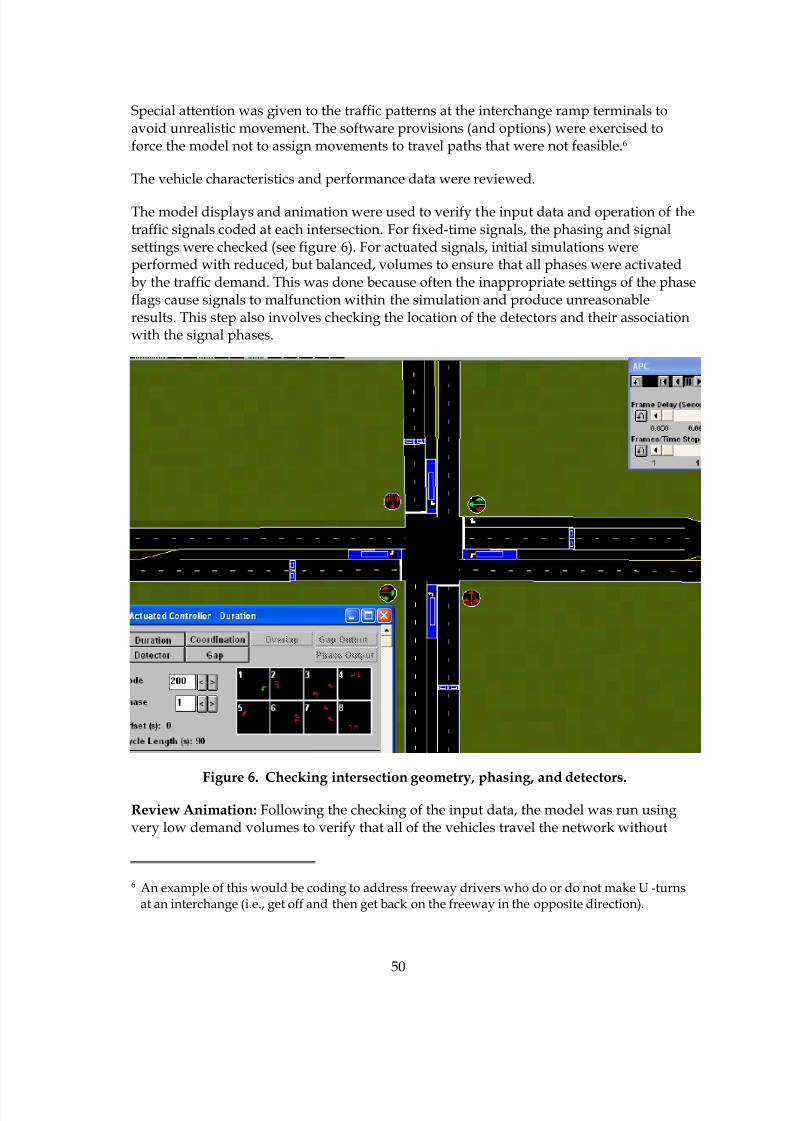
8/8/2019 Vol3 Guidelines
http://slidepdf.com/reader/full/vol3-guidelines 60/146
50
Special attention was given to the traffic patterns at the interchange ramp terminals toavoid unrealistic movement. The software provisions (and options) were exercised toforce the model not to assign movements to travel paths that were not feasible.6
The vehicle characteristics and performance data were reviewed.
The model displays and animation were used to verify the input data and operation of thetraffic signals coded at each intersection. For fixed-time signals, the phasing and signalsettings were checked (see figure 6). For actuated signals, initial simulations wereperformed with reduced, but balanced, volumes to ensure that all phases were activatedby the traffic demand. This was done because often the inappropriate settings of the phaseflags cause signals to malfunction within the simulation and produce unreasonableresults. This step also involves checking the location of the detectors and their associationwith the signal phases.
Figure 6. Checking intersection geometry, phasing, and detectors.
Review Animation: Following the checking of the input data, the model was run usingvery low demand volumes to verify that all of the vehicles travel the network without
6 An example of this would be coding to address freeway drivers who do or do not make U-turnsat an interchange (i.e., get off and then get back on the freeway in the opposite direction).

8/8/2019 Vol3 Guidelines
http://slidepdf.com/reader/full/vol3-guidelines 61/146
51
slowdowns. This step uncovered minor errors in the links alignments that needed to beadjusted.
Next, the traffic demands were specified to about 50 percent of the actual volumes and thesimulation model was rerun. Animation was used to verify that all demands were
properly loaded in the network links and the traffic signals were properly operating. Thelink and system performance measures (travel time, delay) were also checked forreasonableness (i.e., they should reflect free-flow conditions).
Careful checking of the animation revealed subtle coding problems. For example, thecoded distance of a warning sign (for exiting vehicles) or the distance from the start of thelink to the lane drop affects the proper simulation of driver behavior. These problemswere corrected.
Key Decision Point: The model, as revised throughout the error-checking process, wasrun with all the input data (actual demands) and the default model parameters. The
output and animation were also reviewed and discussed with other agency staff whowere familiar with the study area. The conclusion is that the model is working properly.

8/8/2019 Vol3 Guidelines
http://slidepdf.com/reader/full/vol3-guidelines 62/146
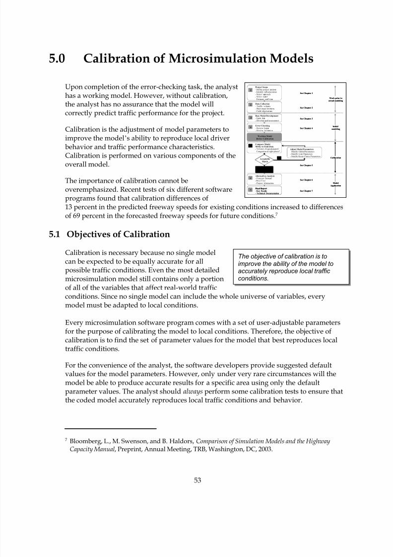
8/8/2019 Vol3 Guidelines
http://slidepdf.com/reader/full/vol3-guidelines 63/146
53
No
Data Collection
- Traffic volumes- Base maps/inventory- Field observations
2
1
Project Scope
- Define project purpose- Identify influence areas- Select approach
- Select model- Estimate staff time
See Chapter 1
See Chapter 2
See Chapter 3
See Chapter 4
Work prior to
actual modeling
Initial
modeling
Yes
Calibrated Model
See Chapter 5
Calibration
See Chapter 6
See Chapter 7
Model
Application
Base Model Development
- Input data- Develop qualityassurance
3
Error Checking
- Review Inputs- Review Animation
4
Compare ModelMOEs to Field Data
- Volumes & speedsmatch?- Congestion in right places?
5
Alternatives Analysis
- Forecast Demand-Base Case- Project Alternatives
6
Final Report
- Key Results- Technical Documentation
7
Working Model
Before Calibration
Acceptable
Match
Adjust Model Parameters
- Modify Global Parameters- Modify Link Parameters- Modify Route Choice Parameters
5.0 Calibration of Microsimulation Models
Upon completion of the error-checking task, the analyst
has a working model. However, without calibration,the analyst has no assurance that the model willcorrectly predict traffic performance for the project.
Calibration is the adjustment of model parameters toimprove the model’s ability to reproduce local driverbehavior and traffic performance characteristics.Calibration is performed on various components of theoverall model.
The importance of calibration cannot beoveremphasized. Recent tests of six different softwareprograms found that calibration differences of13 percent in the predicted freeway speeds for existing conditions increased to differencesof 69 percent in the forecasted freeway speeds for future conditions.7
5.1 Objectives of Calibration
Calibration is necessary because no single modelcan be expected to be equally accurate for allpossible traffic conditions. Even the most detailedmicrosimulation model still contains only a portionof all of the variables that affect real-world trafficconditions. Since no single model can include the whole universe of variables, everymodel must be adapted to local conditions.
Every microsimulation software program comes with a set of user-adjustable parametersfor the purpose of calibrating the model to local conditions. Therefore, the objective ofcalibration is to find the set of parameter values for the model that best reproduces localtraffic conditions.
For the convenience of the analyst, the software developers provide suggested defaultvalues for the model parameters. However, only under very rare circumstances will themodel be able to produce accurate results for a specific area using only the default
parameter values. The analyst should always perform some calibration tests to ensure thatthe coded model accurately reproduces local traffic conditions and behavior.
7 Bloomberg, L., M. Swenson, and B. Haldors, Comparison of Simulation Models and the HighwayCapacity Manual, Preprint, Annual Meeting, TRB, Washington, DC, 2003.
The objective of calibration is toimprove the ability of the model toaccurately reproduce local traffic conditions.

8/8/2019 Vol3 Guidelines
http://slidepdf.com/reader/full/vol3-guidelines 64/146
54
The fundamental assumption of calibration is that the travel behavior models in thesimulation model are essentially sound.8 There is no need to verify that they produce thecorrect delay, travel time, and density when they are given the correct input parametersfor a link. Therefore, the only remaining task for the analyst is to adjust the parameters sothat the models correctly predict local traffic conditions.
5.2 Calibration Approach
Calibration involves the review and adjustment of potentially hundreds of modelparameters, each of which impacts the simulation results in a manner that is often highlycorrelated with that of the others. The analyst can easily get trapped in a never-endingcircular process, fixing one problem only to find that a new one occurs somewhere else.Therefore, it is essential to break the calibration process into a series of logical, sequentialsteps—a strategy for calibration.
To make calibration practical, the parameters must be divided into categories and each
category must be dealt with separately. The analyst should divide the available calibrationparameters into the following two basic categories:
• Parameters that the analyst is certain about and does not wish to adjust.
• Parameters that the analyst is less certain about and willing to adjust.
The analyst should attempt to keep the set of adjustable parameters as small as possible tominimize the effort required to calibrate them. Whenever practical, the analyst should useobserved field data to reflect local conditions. This observed data will serve as thenonadjustable values for certain calibration parameters, thus leaving the set of adjustable
parameters to a minimum. However, the tradeoff is that more parameters allow theanalyst more degrees of freedom to better fit the calibrated model to the specific location.
The set of adjustable parameters is then further subdivided into those that directly impactcapacity (such as mean headway) and those that directly impact route choice. The capacityadjustment parameters are calibrated first, then the route choice adjustment parametersare calibrated.
Each set of adjustable parameters can be further subdivided into those that affect thesimulation on a global basis and those that affect the simulation on a more localizedbasis. The global parameters are calibrated first. The local link-specific parameters areused after the global calibration to fine-tune the results.
8 The analyst determines the soundness of the simulation software when selecting it for use in thestudy.

8/8/2019 Vol3 Guidelines
http://slidepdf.com/reader/full/vol3-guidelines 65/146
55
Capacity calibration has two phases:
1. Global calibration
2. Link fine-tuning
Calibration Strategy:
1. Calibrate capacity parameters.
2. Calibrate route choice parameters.
3. Calibrate overall model performance.
The following three-step strategy is recommended for calibration:
1. Capacity Calibration: An initial calibration isperformed to identify the values for thecapacity adjustment parameters that cause the
model to best reproduce observed trafficcapacities in the field. A global calibration isperformed first, followed by link-specific fine-tuning. The HCM can be used as an alternativesource of capacity target values if fieldmeasurements are not feasible.
2. Route Choice Calibration: If the microsimulation model includes parallel streets, thenroute choice will be important. In this case, a second calibration process is performed,but this time with the route choice parameters. A global calibration is performed first,followed by link-specific fine-tuning.
3. System Performance Calibration: Finally, the overall model estimates of systemperformance (travel times and queues) are compared to the field measurements fortravel times and queues. Fine-tuning adjustments are made to enable the model tobetter match the field measurements.
5.3 Step 1: Calibration for Capacity
The capacity calibration step adjusts the global and link-specific capacity-relatedparameters in the simulation model to best replicate local field measurements for capacity.This is an important step because capacity has a significant effect on predicted system
performance (delay and queues).9
The objective of this calibration step is to find a set ofmodel parameters that causes the model to come as close as possible to matching the fieldmeasurements for traffic capacity.
The capacity calibration step consists of two phases:(1) a global calibration phase and (2) a fine-tuningphase. Global calibration is first performed toidentify the appropriate network-wide value of thecapacity parameter(s) that best reproduces
9 Historically, it has been the practice to calibrate microsimulation models to all the traffic counts inthe field. The majority of these counts will be at noncritical locations. The recommended strategyis to focus (at this point in the calibration process) only on the critical counts at the bottlenecksand to get the model to reproduce these counts correctly. Once this has been done, the rest of thecounts are used later to check the route choice aspects of the model. All of this presupposes thatthe demands have been entered correctly and have already been checked against the counts at theentry gates as part of the first step (error checking).

8/8/2019 Vol3 Guidelines
http://slidepdf.com/reader/full/vol3-guidelines 66/146
8/8/2019 Vol3 Guidelines
http://slidepdf.com/reader/full/vol3-guidelines 67/146
57
If the model initially shows no
congestion at the bottlenecks, thedemand must be temporarily increased before calibration can
proceed.
All “false” bottlenecks in the model must be cleared before calibrationcan proceed.
where:
c = capacity (vehicles per hour (veh/h))
s = saturation flow (veh/h per green phase)
g = effective green timeC = cycle length
Higher saturation flows and lower startup lost times result in higher capacities.
Several measurements of maximum flow rates should be made in the field and averaged.Procedures are provided in the appendix for estimating how many measurements arerequired to estimate capacity within a desired confidence interval (see Appendix B:Confidence Intervals). If capacity cannot be measured in the field, then the HCMmethodology can be used to estimate capacity. The HCM methods should not beconsidered a default technique since the estimates are not as accurate as direct field
measurements.
5.3.2 Obtain Model Estimates of Capacity
Microsimulation models do not output a number called “capacity.” Instead, they outputthe number of vehicles that pass a given point. Thus, the analyst must manipulate theinput demand as necessary to create a queue upstream of the target section to becalibrated so that the model will report the maximum possible flow rate through thebottleneck.
If the model does not initially show congestion at
the same bottleneck locations as exist in the field,then the demands coded in the model aretemporarily increased to force the creation ofcongestion at those bottlenecks. These temporaryincreases must be removed after the capacitycalibration has been completed, but before the route choice calibration step.
If the model initially shows congested bottlenecks atlocations that DO NOT exist in the field, it will benecessary to temporarily increase the capacity atthose false bottlenecks (using temporary link-specific
headway adjustments). These temporary adjustments are then removed during the fine-tuning phase.
For nonsignalized facilities (freeways, rural highways, and rural roads), the simulatedqueue should persist for at least 15 min of simulated time, across all lanes and linksfeeding the target section. The simulated capacity is then the mean flow rate at the targetsection (measured at a detector placed in the target section and summed across all lanes)averaged over the 15-min or longer period that the queue is present. The result is thendivided by the number of lanes and is converted to an hourly flow rate.
8/8/2019 Vol3 Guidelines
http://slidepdf.com/reader/full/vol3-guidelines 68/146
58
Mean headway is a good global parameter for calibrating capacity. It may have different names indifferent software.
For signalized intersections, the coded demand should be increased, as necessary, toensure the necessary queues of at least 10 vehicles at the start of the green phase. Adetector is placed in the model at the stop line to measure the discharge headways (on aper lane basis) of the first 10 vehicles crossing the detector in each lane.11 The per laneheadways are averaged for each lane and then averaged across lanes. The result is then
converted to an hourly flow rate per lane.
Just as the field measurements of capacity were repeated several times and the resultswere averaged, the model runs should be repeated several times and the maximum flowrate at each location should be averaged across the runs. The minimum required numberof runs to obtain a value of capacity within a desired confidence interval can be calculatedusing the procedures provided in appendix B (Confidence Intervals).
5.3.3 Select Calibration Parameter(s)
Only the model parameters that directly affect capacity are calibrated at this time. Each
microsimulation software program has its own set of parameters that affect capacity,depending on the specific car-following and lane-changing logic implemented in thesoftware. The analyst must review the software documentation and select one or two ofthese parameters for calibration.
This chapter does not intend to describe all of the parameters for all of the simulationmodels that are available. An illustrative list of capacity-related parameters for freewaysand signalized arterials is given below:
Freeway Facilities:
• Mean following headway.• Driver reaction time.
• Critical gap for lane changing.
• Minimum separation under stop-and-go conditions.
Signalized Intersections:
• Startup lost time.
• Queue discharge headway.
• Gap acceptance for unprotected left turns.
For example, in CORSIM, the two parameters thatmost globally affect capacity are “headway factor byvehicle type” (record type 58) and “car following
11The headways for the first three vehicles are discarded.
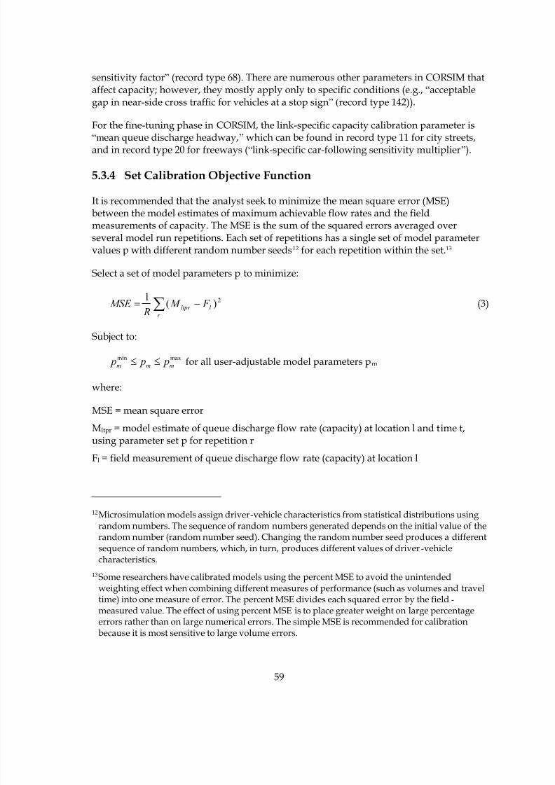
8/8/2019 Vol3 Guidelines
http://slidepdf.com/reader/full/vol3-guidelines 69/146
59
sensitivity factor” (record type 68). There are numerous other parameters in CORSIM thataffect capacity; however, they mostly apply only to specific conditions (e.g., “acceptablegap in near-side cross traffic for vehicles at a stop sign” (record type 142)).
For the fine-tuning phase in CORSIM, the link-specific capacity calibration parameter is
“mean queue discharge headway,” which can be found in record type 11 for city streets,and in record type 20 for freeways (“link-specific car-following sensitivity multiplier”).
5.3.4 Set Calibration Objective Function
It is recommended that the analyst seek to minimize the mean square error (MSE)between the model estimates of maximum achievable flow rates and the fieldmeasurements of capacity. The MSE is the sum of the squared errors averaged overseveral model run repetitions. Each set of repetitions has a single set of model parametervalues p with different random number seeds12 for each repetition within the set.13
Select a set of model parameters p to minimize:
∑ −=r
l ltpr F M R
MSE 2)(1
(3)
Subject to:
maxmin
mmm p p p ≤≤ for all user-adjustable model parameters pm
where:
MSE = mean square errorMltpr = model estimate of queue discharge flow rate (capacity) at location l and time t,using parameter set p for repetition r
Fl = field measurement of queue discharge flow rate (capacity) at location l
12Microsimulation models assign driver-vehicle characteristics from statistical distributions usingrandom numbers. The sequence of random numbers generated depends on the initial value of therandom number (random number seed). Changing the random number seed produces a different
sequence of random numbers, which, in turn, produces different values of driver-vehiclecharacteristics.
13Some researchers have calibrated models using the percent MSE to avoid the unintendedweighting effect when combining different measures of performance (such as volumes and traveltime) into one measure of error. The percent MSE divides each squared error by the field-
measured value. The effect of using percent MSE is to place greater weight on large percentageerrors rather than on large numerical errors. The simple MSE is recommended for calibrationbecause it is most sensitive to large volume errors.

8/8/2019 Vol3 Guidelines
http://slidepdf.com/reader/full/vol3-guidelines 70/146
60
R = number of repetitive model runs with fixed parameter values pm and differentrandom number seeds14
pm = value of model parameter number m
pmmin, pmmax = user-specified limits to the allowable range of parameter values pm (limits
are necessary to avoid solutions that violate the laws of physics, vehicle performancelimits, and driver behavior extremes)
5.3.5 Perform Search for Optimal Parameter Value
The analyst must now find the capacity adjustment factor(s) p that minimizes the MSEbetween the model and the field measurements of capacity. The calibration problem is anonlinear least-squares optimization problem.
Since simulation models are complex, it is not usually possible to formulate the models asa closed-form equation for which traditional calculus techniques can be applied to find a
minimum value solution. It is necessary to use some sort of search algorithm that relies onmultiple operations of the simulation model, plotting of the output results as points, andsearching between these points for the optimal solution. Search algorithms are required tofind the optimal solution to the calibration problem.
There are many software programs available for identifying the optimal combination ofcalibration parameters for minimizing the squared error between the field observationsand the simulation model. The Optimization Technology Center Web site of the ArgonneNational Laboratory and Northwestern University lists several software programs fornonlinear least-squares parameter estimation. See the following:
www-fp.mcs.anl.gov/otc/Guide/SoftwareGuide/Categories/nonlinleastsq.html
Appendix D describes a few simple search algorithms that can be applied manually orwith the aid of spreadsheets. Figure 7 illustrates how a single parameter search (m = 1)might look using one of these simple search algorithms for the number of model runs (R)set to 4.
14Since the objective is to minimize error, dividing by a constant R (the number of repetitions)would have no effect on the results. However, R is included in the objective function toemphasize to the analyst the necessity of running the model several times with each parameterset.
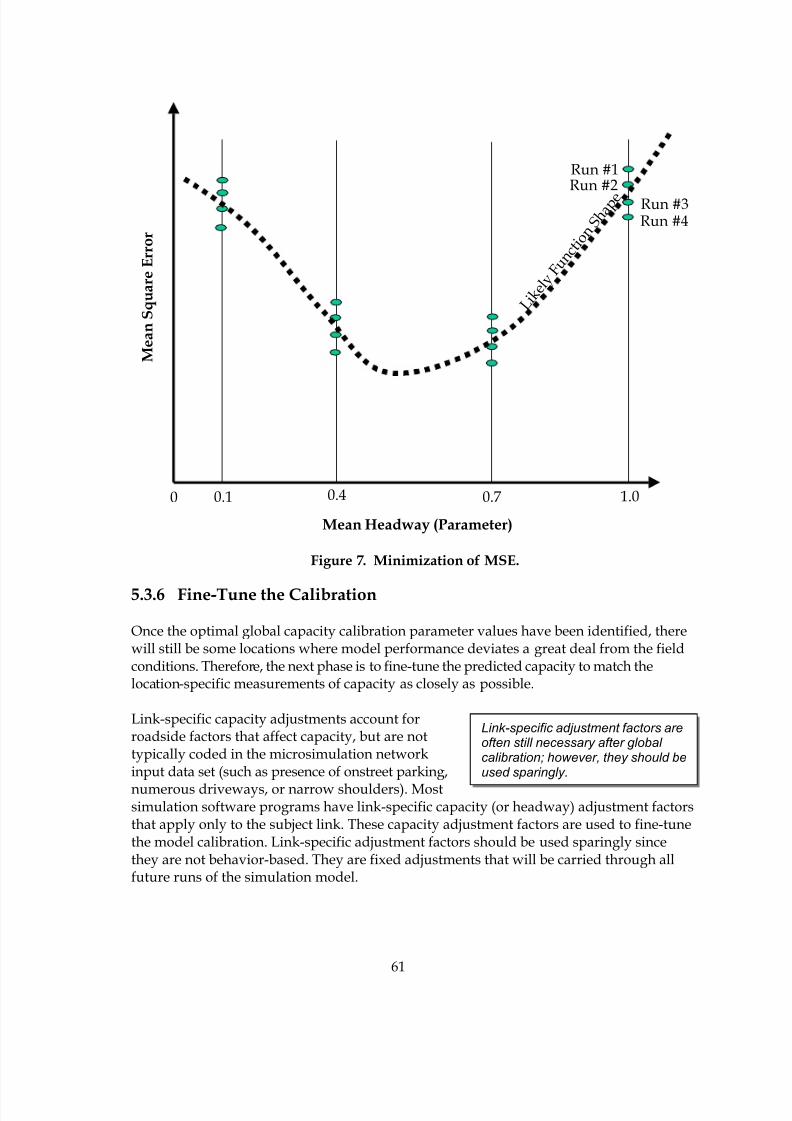
8/8/2019 Vol3 Guidelines
http://slidepdf.com/reader/full/vol3-guidelines 71/146
61
Link-specific adjustment factors areoften still necessary after global calibration; however, they should beused sparingly.
0 0.4 0.7
M e a n S q u a r e E r r o r
Mean Headway (Parameter)
0.1 1.0
Run #1Run #2
Run #3Run #4
L i k e
l y F u n c
t i o n S h
a p e
Figure 7. Minimization of MSE.
5.3.6 Fine-Tune the Calibration
Once the optimal global capacity calibration parameter values have been identified, therewill still be some locations where model performance deviates a great deal from the fieldconditions. Therefore, the next phase is to fine-tune the predicted capacity to match thelocation-specific measurements of capacity as closely as possible.
Link-specific capacity adjustments account forroadside factors that affect capacity, but are nottypically coded in the microsimulation networkinput data set (such as presence of onstreet parking,
numerous driveways, or narrow shoulders). Mostsimulation software programs have link-specific capacity (or headway) adjustment factorsthat apply only to the subject link. These capacity adjustment factors are used to fine-tunethe model calibration. Link-specific adjustment factors should be used sparingly sincethey are not behavior-based. They are fixed adjustments that will be carried through allfuture runs of the simulation model.

8/8/2019 Vol3 Guidelines
http://slidepdf.com/reader/full/vol3-guidelines 72/146

8/8/2019 Vol3 Guidelines
http://slidepdf.com/reader/full/vol3-guidelines 73/146
63
5.5 Step 3: System Performance Calibration
In this last step of the calibration, the overall traffic performance predicted by the fullyfunctioning model is compared to the field measurements of travel time, queue lengths,and the duration of queuing. The analyst refines link free-flow speeds and link capacitiesto better match the field conditions. Since changes made at this step may compromise theprior two steps of calibration, these changes should be made sparingly. The next sectionsuggests calibration targets for this last step of the review.
5.6 Calibration Targets
The objective of model calibration is to obtain the best match possible between modelperformance estimates and the field measurements of performance. However, there is alimit to the amount of time and effort anyone can put into eliminating error in the model.There comes a point of diminishing returns where large investments in effort yield smallimprovements in accuracy. The analyst needs to know when to stop. This is the purposeof adopting calibration targets for the model.
Calibration targets are developed based on the minimum performance requirements forthe microsimulation model, taking into consideration the available resources. The targetswill vary according to the purpose for which the microsimulation model is beingdeveloped and the resources available to the analyst.
Table 4 provides an example of calibration targets that were developed by Wisconsin DOTfor their Milwaukee freeway system simulation model. They are based on guidelinesdeveloped in the United Kingdom.18
18 “Traffic Appraisal in Urban Areas, Highways Agency,” Design Manual for Roads and Bridges:Volume 12, Section 2, Department for Transport (formerly Department of Environment, Transport,and the Regions), London, England, May 1996 (www.official-documents.co.uk/document/deps/ha/dmrb/index.htm)
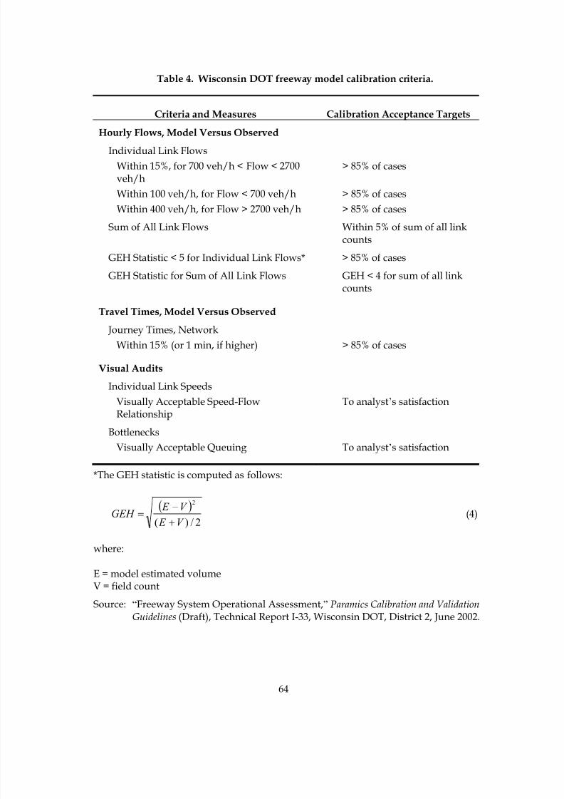
8/8/2019 Vol3 Guidelines
http://slidepdf.com/reader/full/vol3-guidelines 74/146
64
Table 4. Wisconsin DOT freeway model calibration criteria.
Criteria and Measures Calibration Acceptance Targets
Hourly Flows, Model Versus Observed
Individual Link Flows
Within 15%, for 700 veh/h < Flow < 2700veh/h
> 85% of cases
Within 100 veh/h, for Flow < 700 veh/h > 85% of cases
Within 400 veh/h, for Flow > 2700 veh/h > 85% of cases
Sum of All Link Flows Within 5% of sum of all linkcounts
GEH Statistic < 5 for Individual Link Flows* > 85% of cases
GEH Statistic for Sum of All Link Flows GEH < 4 for sum of all linkcounts
Travel Times, Model Versus Observed
Journey Times, Network
Within 15% (or 1 min, if higher) > 85% of cases
Visual Audits
Individual Link Speeds
Visually Acceptable Speed-Flow
Relationship
To analyst’s satisfaction
Bottlenecks
Visually Acceptable Queuing To analyst’s satisfaction
*The GEH statistic is computed as follows:
( )2/)(
2
V E
V E GEH
+
−= (4)
where:
E = model estimated volumeV = field count
Source: “Freeway System Operational Assessment,” Paramics Calibration and ValidationGuidelines (Draft), Technical Report I-33, Wisconsin DOT, District 2, June 2002.

8/8/2019 Vol3 Guidelines
http://slidepdf.com/reader/full/vol3-guidelines 75/146
65
Another example of suggested calibration targets is “Theil’s Inequality Coefficient,” whichis broken down into three parts, each of which provides information on the differencesbetween the model measures and the target measures.19
5.7 Example Problem: Model Calibration
The same example problem from the previous chapters is continued. The task is now tocalibrate the model.
A review of the results produced by the working model at the end of the modeldevelopment task indicates that there are discrepancies between the observed andsimulated traffic performance. The purpose of the calibration process is to adjust themodel parameters to better match field conditions.
Calibration for Capacity—Step 1: Global Calibration
Field Data on Capacity: The network under study is not congested. Therefore, fieldmeasurements of the capacity values on the freeway links and saturation flows at thetraffic signals on the arterials cannot be obtained.
Two potential future bottleneck locations were selected on the study area network. Thecapacities for these potential bottleneck locations were estimated using the HCM 2000procedures. The estimated value for the saturation flow for protected movements atsignalized intersections was 1800 vehicles per hour of green per lane (vphgpl) and thecapacity of the freeway links was 2100 vphgpl.
Model Estimates of Capacity: The model estimates of capacity can be obtained from
detector measurements or from the throughput values reported at the end of thesimulation run. However, it is necessary to have upstream queues for the throughputvalues to represent capacity.
Because of the lack of congestion, the existing volumes on the network links had to beartificially increased to trigger congestion upstream of the bottleneck locations (the modelthroughput volumes at these bottleneck locations would then be the model-estimatedcapacities).
Select Calibration Parameters: The global parameter calibration was performed using thefollowing parameters:
• Mean queue discharge headway at traffic signals: The default value for this parameterin the model is 1.8 s/veh (which is equivalent to a saturation flow of 2000 vphgpl
19Further discussions of Theil’s Inequality Coefficient can be found in the Advanced CORSIM Training Manual, Minnesota DOT, 2002, and in Hourdakis, J., P. Michalopoulos, and J.Kottommannil, “Practical Procedure for Calibrating Microscopic Traffic Simulation Models,” TRB,TRR 1852, Washington, D.C., 2003.
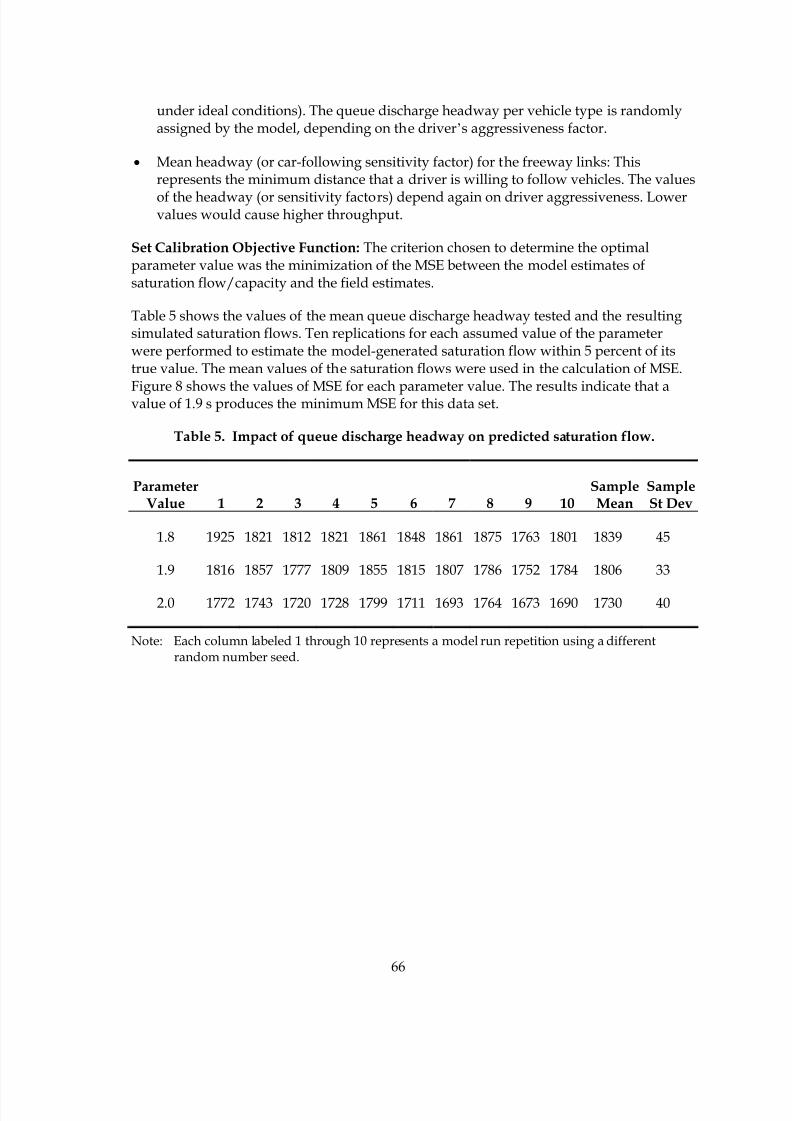
8/8/2019 Vol3 Guidelines
http://slidepdf.com/reader/full/vol3-guidelines 76/146
66
under ideal conditions). The queue discharge headway per vehicle type is randomlyassigned by the model, depending on the driver’s aggressiveness factor.
• Mean headway (or car-following sensitivity factor) for the freeway links: Thisrepresents the minimum distance that a driver is willing to follow vehicles. The values
of the headway (or sensitivity factors) depend again on driver aggressiveness. Lowervalues would cause higher throughput.
Set Calibration Objective Function: The criterion chosen to determine the optimalparameter value was the minimization of the MSE between the model estimates ofsaturation flow/capacity and the field estimates.
Table 5 shows the values of the mean queue discharge headway tested and the resultingsimulated saturation flows. Ten replications for each assumed value of the parameterwere performed to estimate the model-generated saturation flow within 5 percent of itstrue value. The mean values of the saturation flows were used in the calculation of MSE.
Figure 8 shows the values of MSE for each parameter value. The results indicate that avalue of 1.9 s produces the minimum MSE for this data set.
Table 5. Impact of queue discharge headway on predicted saturation flow.
ParameterValue 1 2 3 4 5 6 7 8 9 10
SampleMean
SampleSt Dev
1.8 1925 1821 1812 1821 1861 1848 1861 1875 1763 1801 1839 45
1.9 1816 1857 1777 1809 1855 1815 1807 1786 1752 1784 1806 33
2.0 1772 1743 1720 1728 1799 1711 1693 1764 1673 1690 1730 40
Note: Each column labeled 1 through 10 represents a model run repetition using a differentrandom number seed.
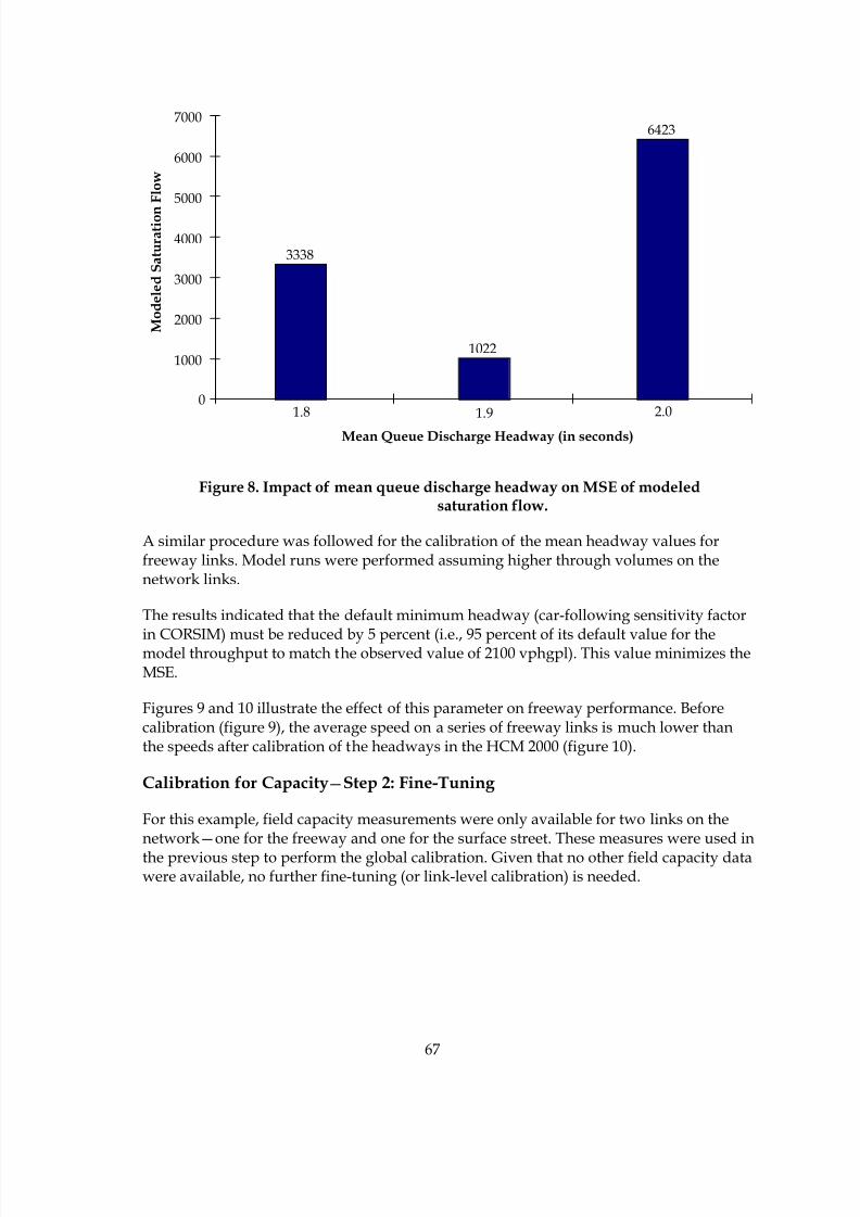
8/8/2019 Vol3 Guidelines
http://slidepdf.com/reader/full/vol3-guidelines 77/146
67
3338
1022
6423
2.01.91.80
1000
2000
3000
4000
5000
6000
7000
Mean Queue Discharge Headway (in seconds)
M o d e l e d S a t u r a t i o n
F l o w
Figure 8. Impact of mean queue discharge headway on MSE of modeledsaturation flow.
A similar procedure was followed for the calibration of the mean headway values forfreeway links. Model runs were performed assuming higher through volumes on thenetwork links.
The results indicated that the default minimum headway (car-following sensitivity factor
in CORSIM) must be reduced by 5 percent (i.e., 95 percent of its default value for themodel throughput to match the observed value of 2100 vphgpl). This value minimizes theMSE.
Figures 9 and 10 illustrate the effect of this parameter on freeway performance. Beforecalibration (figure 9), the average speed on a series of freeway links is much lower thanthe speeds after calibration of the headways in the HCM 2000 (figure 10).
Calibration for Capacity—Step 2: Fine-Tuning
For this example, field capacity measurements were only available for two links on thenetwork—one for the freeway and one for the surface street. These measures were used in
the previous step to perform the global calibration. Given that no other field capacity datawere available, no further fine-tuning (or link-level calibration) is needed.
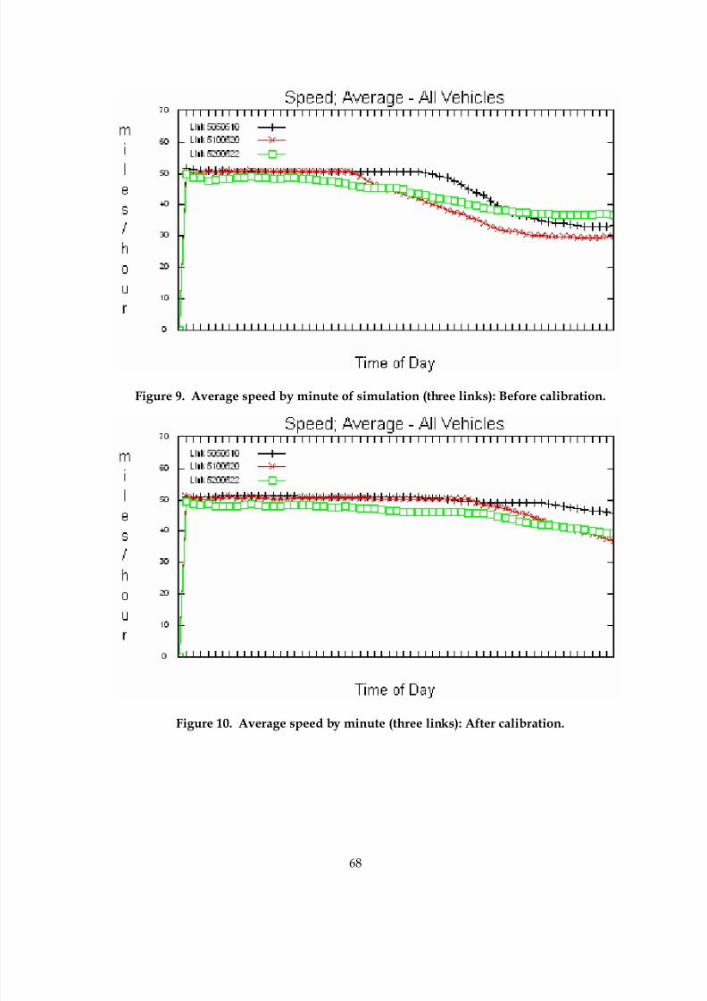
8/8/2019 Vol3 Guidelines
http://slidepdf.com/reader/full/vol3-guidelines 78/146

8/8/2019 Vol3 Guidelines
http://slidepdf.com/reader/full/vol3-guidelines 79/146
69
Calibration for Route Choice
The prior calibration step has ensured that the model is predicting the correct capacities.With the correct capacities, the model should no longer have bottlenecks at the incorrectlocations with too low or too high discharge rates. The upstream and downstream traffic
volumes on each of the links should now better match the observed counts. Any remainingdifferences (assuming that error checking caught errors in the source node volumes)should be the result of route choice errors in the model. Therefore, the purpose of routechoice calibration is to better match the counts at the non-bottleneck locations on thenetwork.
The particular software selected for this example problem does not predict changes inroute choice (no O-D table was provided for the model). Therefore, there is no routechoice to be calibrated.20 Assuming that the analyst is confident in the quality of the turncounts entered into the model (and converted inside the model into equivalent turnprobabilities for routing traffic), any remaining errors in the link volumes can be corrected
by manual adjustments to midblock source and sink node volumes.
In this example problem, the freeway, ramp, and intersection counts were all adjusted atthe data preparation stage to produce an internally consistent set of volumes for every linkand node. There are no unaccounted for increases or decreases in volumes between nodes.Thus, no midblock source/sink nodes were required. The model-predicted link volumesbased on the source node volumes and the intersection turn percentages are consistentwith the link counts (within the range of variation expected because of the randomcomponents of the simulation model).
System Performance Calibration
Once calibration has been completed to the analyst’s satisfaction, the next step is tocalibrate the overall performance of the model.
The model predictions were compared with the field data on speed, travel time, and delayon the freeways and arterials.
Based on this comparison, the free-flow speed distribution for the freeway was adjustedso that the model-generated free-flow speeds were within a more narrow range than thedefault distribution. This reflects commuter traffic behavior.
No other adjustments were made to the model parameters.
20Actually, the analyst could (in theory) calibrate the percentage turns that were input at eachintersection and ramp junction to better match the observed link flows downstream from thesource nodes; however, this is currently impractical (there are too many variables to be adjustedwithout the assistance of a good computerized optimization algorithm).

8/8/2019 Vol3 Guidelines
http://slidepdf.com/reader/full/vol3-guidelines 80/146
70
Ten repetitions of the calibrated data set were performed and the link output wasprocessed to produce performance measures to be compared with the field data.
The comparison is shown in table 6. The simulated values represent the mean value of theMOEs based on the 10 model runs for the third time slice of the simulated peak hour.
Comparisons with field measurement of delay are not shown here because it was unclearhow the field data on delay were collected. In general, users must be cautious when theycompare field versus simulated delays because the delay is typically defined differently inmost software programs than in the approaches commonly used for field measurements.
The results indicate that the model satisfies the criteria for calibration (shown in table 4).
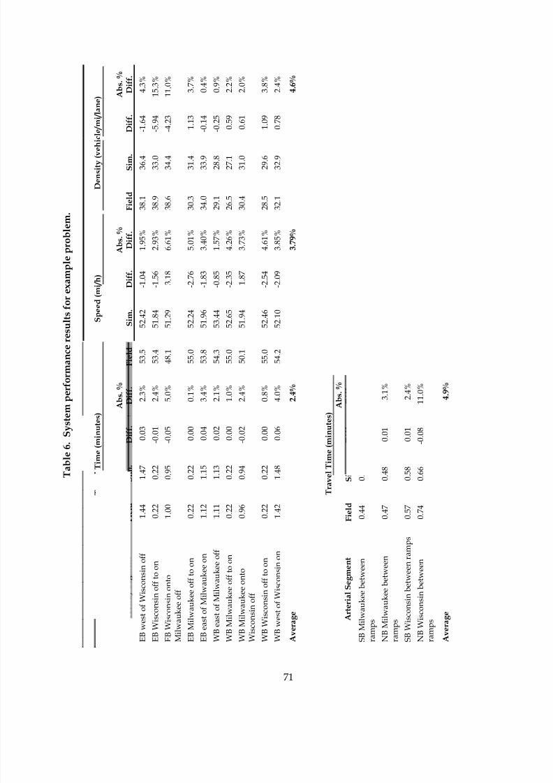
8/8/2019 Vol3 Guidelines
http://slidepdf.com/reader/full/vol3-guidelines 81/146
T a b l e 6 . S y s t e m
p e r f o r m a n c e r e s u l t s f o r e x a m
p l e p r o b l e m .
T r a v e l T i m e ( m i n u t e s )
S p e e d ( m i / h )
D e n s i t y ( v e h i c l e / m i / l a n e )
F r e e w a y S e g m e n t
F i e l d
S i m .
D i f f .
A b s . %
D i f f .
F i e l d
S i m .
D i f f .
A b s . %
D i f f .
F i e l d
S i m .
D i f f .
A b s . %
D i f f .
E B w e s t o f W i s c o n s i n o f f
1 . 4 4
1 . 4 7
0 . 0 3
2 . 3 %
5 3 . 5
5 2 . 4 2
- 1 . 0 4
1 . 9 5 %
3 8 . 1
3 6 . 4
- 1 . 6 4
4 . 3 %
E B W i s c o n s i n o f f t o o n
0 . 2 2
0 . 2 2
- 0 . 0 1
2 . 4 %
5 3 . 4
5 1 . 8 4
- 1 . 5 6
2 . 9 3 %
3 8 . 9
3 3 . 0
- 5 . 9 4
1 5 . 3 %
E B W i s c o n s i n o n t o
M i l w a u k e e o f f
1 . 0 0
0 . 9 5
- 0 . 0 5
5 . 0 %
4 8 . 1
5 1 . 2 9
3 . 1 8
6 . 6 1 %
3 8 . 6
3 4 . 4
- 4 . 2 3
1 1 . 0 %
E B M i l w a u k e e o f f t o o n
0 . 2 2
0 . 2 2
0 . 0 0
0 . 1 %
5 5 . 0
5 2 . 2 4
- 2 . 7 6
5 . 0 1 %
3 0 . 3
3 1 . 4
1 . 1 3
3 . 7 %
E B e a s t o f M i l w a u k e e o n
1 . 1 2
1 . 1 5
0 . 0 4
3 . 4 %
5 3 . 8
5 1 . 9 6
- 1 . 8 3
3 . 4 0 %
3 4 . 0
3 3 . 9
- 0 . 1 4
0 . 4 %
W B e a s t o f M i l w a u k e e o f f
1 . 1 1
1 . 1 3
0 . 0 2
2 . 1 %
5 4 . 3
5 3 . 4 4
- 0 . 8 5
1 . 5 7 %
2 9 . 1
2 8 . 8
- 0 . 2 5
0 . 9 %
W B M i l w a u k e e o f f t o o n
0 . 2 2
0 . 2 2
0 . 0 0
1 . 0 %
5 5 . 0
5 2 . 6 5
- 2 . 3 5
4 . 2 6 %
2 6 . 5
2 7 . 1
0 . 5 9
2 . 2 %
W B M i l w a u k e e o n t o
W i s c o n s i n o f f
0 . 9 6
0 . 9 4
- 0 . 0 2
2 . 4 %
5 0 . 1
5 1 . 9 4
1 . 8 7
3 . 7 3 %
3 0 . 4
3 1 . 0
0 . 6 1
2 . 0 %
W B W i s c o n s i n o f f t o o n
0 . 2 2
0 . 2 2
0 . 0 0
0 . 8 %
5 5 . 0
5 2 . 4 6
- 2 . 5 4
4 . 6 1 %
2 8 . 5
2 9 . 6
1 . 0 9
3 . 8 %
W B w e s t o f W i s c o n s i n o n
1 . 4 2
1 . 4 8
0 . 0 6
4 . 0 %
5 4 . 2
5 2 . 1 0
- 2 . 0 9
3 . 8 5 %
3 2 . 1
3 2 . 9
0 . 7 8
2 . 4 %
A v e r a g e
2 . 4 %
3 . 7 9 %
4 . 6 %
T r a v e l T i m e ( m i n u t e s )
A r t e r i a l S e g m e n t
F i e l d
S i m .
D i f f .
A b s . %
D i f f .
S B M i l w a u k e e b e t w e e n
r a m p s
0 . 4 4
0 . 4 3
- 0 . 0 1
3 . 0 %
N B M i l w a u k e e b e t w e e n
r a m p s
0 . 4 7
0 . 4 8
0 . 0 1
3 . 1 %
S B W i s c o n s i n b e t w e e n r a m
p s
0 . 5 7
0 . 5 8
0 . 0 1
2 . 4 %
N B W i s c o n s i n b e t w e e n
r a m p s
0 . 7 4
0 . 6 6
- 0 . 0 8
1 1 . 0 %
A v e r a g e
4 . 9 %
71

8/8/2019 Vol3 Guidelines
http://slidepdf.com/reader/full/vol3-guidelines 82/146
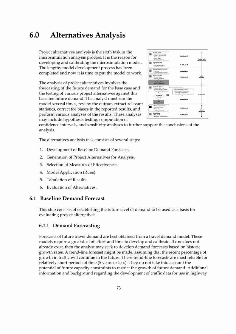
8/8/2019 Vol3 Guidelines
http://slidepdf.com/reader/full/vol3-guidelines 83/146
73
No
Data Collection
- Traffic volumes- Base maps/inventory- Field observations
2
1
Project Scope
- Define project purpose- Identify influence areas- Select approach
- Select model- Estimate staff time
See Chapter 1
See Chapter 2
See Chapter 3
See Chapter 4
Work prior to
actual modeling
Initial
modeling
Yes
Calibrated Model
See Chapter 5
Calibration
See Chapter 6
See Chapter 7
Model
Application
Base Model Development
- Input data- Develop qualityassurance
3
Error Checking
- Review Inputs- Review Animation
4
Compare ModelMOEs to Field Data
- Volumes & speedsmatch?- Congestion in right places?
5
Alternatives Analysis
- Forecast Demand-Base Case- Project Alternatives
6
Final Report
- Key Results- Technical Documentation
7
Working Model
Before Calibration
Acceptable
Match
Adjust Model Parameters
- Modify Global Parameters- Modify Link Parameters- Modify Route Choice Parameters
6.0 Alternatives Analysis
Project alternatives analysis is the sixth task in the
microsimulation analysis process. It is the reason fordeveloping and calibrating the microsimulation model.The lengthy model development process has beencompleted and now it is time to put the model to work.
The analysis of project alternatives involves theforecasting of the future demand for the base case andthe testing of various project alternatives against thisbaseline future demand. The analyst must run themodel several times, review the output, extract relevantstatistics, correct for biases in the reported results, andperform various analyses of the results. These analysesmay include hypothesis testing, computation ofconfidence intervals, and sensitivity analyses to further support the conclusions of theanalysis.
The alternatives analysis task consists of several steps:
1. Development of Baseline Demand Forecasts.
2. Generation of Project Alternatives for Analysis.
3. Selection of Measures of Effectiveness.
4. Model Application (Runs).
5. Tabulation of Results.
6. Evaluation of Alternatives.
6.1 Baseline Demand Forecast
This step consists of establishing the future level of demand to be used as a basis forevaluating project alternatives.
6.1.1 Demand Forecasting
Forecasts of future travel demand are best obtained from a travel demand model. Thesemodels require a great deal of effort and time to develop and calibrate. If one does notalready exist, then the analyst may seek to develop demand forecasts based on historicgrowth rates. A trend-line forecast might be made, assuming that the recent percentage ofgrowth in traffic will continue in the future. These trend-line forecasts are most reliable forrelatively short periods of time (5 years or less). They do not take into account thepotential of future capacity constraints to restrict the growth of future demand. Additionalinformation and background regarding the development of traffic data for use in highway

8/8/2019 Vol3 Guidelines
http://slidepdf.com/reader/full/vol3-guidelines 84/146
74
planning and design may be found in National Cooperative Highway Research Program(NCHRP) Report 255, Highway Traffic Data for Urbanized Area Project Planning and Design.
6.1.2 Constraining Demand to Capacity
Regardless of which method is used to estimate future demand (regional model or trendline), care must be taken to ensure that the forecasts are a reasonable estimate of the actualamount of traffic that can arrive within the analytical period at the study area. Regionalmodel forecasts are usually not well constrained to system capacity and trend-lineforecasts are totally unconstrained. Appendix F provides a method for constraining futuredemands to the physical ability of the transportation system to deliver the traffic to themicrosimulation model study area.
6.1.3 Allowance for Uncertainty in Demand Forecasts
All forecasts are subject to uncertainty. It is risky to design a road facility to a precise
future condition given the uncertainties in the forecasts. There are uncertainties in boththe probable growth in demand and the available capacity that might be present in thefuture. Slight changes in the timing or design of planned or proposed capacityimprovements outside of the study area can significantly change the amount of trafficdelivered to the study area during the analytical period. Changes in future vehicle mixand peaking can easily affect capacity by 10 percent. Similarly, changes in economicdevelopment and public agency approvals of new development can significantly changethe amount of future demand. Thus, it is good practice to explicitly plan for a certainamount of uncertainty in the analysis. This level of uncertainty is the purpose ofsensitivity testing (explained in a separate section below).
6.2 Generation of Alternatives
In this step, the analyst generates improvement alternatives based on direction from thedecisionmakers and through project meetings. They will probably reflect operationalstrategies and/or geometric improvements to address the problems identified based onthe baseline demand forecasts. The specifics of alternatives generation are beyond thescope of this report. Briefly, they consist of:
• Performing a microsimulation analysis1 of the baseline demand forecast to identify thedeficiencies.2
• Identifying alternative improvements that solve one or more of the identified problems.3
1 A sketch-planning analysis using HCM techniques can be performed, if desired, to identifyconceptual project alternatives prior to the development of a calibrated simulation model. Thecalibrated simulation model can then be used to refine the conceptual plans.
2 Deficiencies are identified by comparing the measured performance against the project objectivesand agency performance standards identified in task 1 (Project Scope).
8/8/2019 Vol3 Guidelines
http://slidepdf.com/reader/full/vol3-guidelines 85/146
75
When reviewing model output, theanalyst should look at a few key systemwide performance measures
plus “hot spots” (indicators of localized breakdowns in the system).
6.3 Selection of Measures of Effectiveness (MOEs)
MOEs are the system performance statistics thatbest characterize the degree to which a particularalternative meets the project objectives (which weredetermined in the Project Scope task). Thus, theappropriate MOEs are determined by the projectobjectives and agency performance standards ratherthan what is produced by the model. This section, however, discusses what output istypically produced by microsimulation software so that the analyst can appreciate whatoutput might be available for constructing the desired MOEs.
Microsimulation, by its very nature, can bury the analyst in detailed microscopic output.The key is to focus on a few key indicators of system performance and localizedbreakdowns in the system (locations where queues are interfering with systemsoperation).
6.3.1 Candidate MOEs for Overall System Performance
As explained above, the selection of MOEs should be driven by the project objectives andthe agency performance standards; however, many MOEs of overall system performancecan be computed directly or indirectly from the following three basic system performancemeasures:
• Vehicle-miles traveled (VMT) or vehicle-kilometers traveled.
• Vehicle-hours traveled (VHT).
• Mean system speed.
These three basic performance measures can also be supplemented with other modeloutput, depending on the objectives of the analysis. For example, total system delay is auseful overall system performance measure for comparing the congestion-relieving
3 In support of the purpose and scope of the project, this identification of alternatives must takeinto consideration the range of demand conditions, weather conditions, incidents, andoperational management strategies. Additional information and background may be found in thefollowing documents:
Bunch, J., S. Hatcher, J. Larkin, G. Nelson, A. Proper, D. Roberts, V. Shah, and K. Wunderlich,Incorporating ITS Into Corridor Planning: Seattle Case Study, ITS Electronic Document Library(EDL)#11303, August 1999.
Wunderlich, K., Incorporating ITS Into Planning Analyses: Summary of Key Findings From a Seattle2020 Case Study, Report No. FHWA-OP-02-031, May 2002.
8/8/2019 Vol3 Guidelines
http://slidepdf.com/reader/full/vol3-guidelines 86/146
76
effectiveness of various alternatives. The number of stops is a useful indicator for signalcoordination studies.
6.3.2 Candidate MOEs for Localized Problems
In addition to evaluating overall system performance, the analyst should also be evaluatingif and where there are localized system breakdowns (“hot spots”). A hot spot may beindicated by a persistent short queue that lasts too long, a signal phase failure (green timethat fails to clear all waiting vehicles), or a blocked link (queue that backs up onto anupstream intersection).
A blocked link is the most significant indicator of localized breakdowns. A queue ofvehicles that fills a link and blocks an upstream intersection can have a significant impacton system performance. A link queue overflow report can be developed to identify thelinks and times during the simulation period when the computed queue of vehiclesequaled (and, therefore, probably actually exceeded) the storage capacity of the link.4
Signal phase failures, where the provided green time is insufficient to clear the queue,indicate potential operational problems if the queues continue to build over several cycles.The analyst should develop a signal phase failure report to indicate when and wheresignal green times are not sufficient to clear out all of the waiting queues of vehicles duringeach cycle.
At the finest level of detail, the analyst may wish to develop a report of the presence ofpersistent queues of a minimum length. This “hot spot” report would identify persistentqueues on a lane-by-lane basis of a minimum number of vehicles that persist for a minimumamount of time. This report points the analyst to locations of persistent long queues (even
those that do not overflow beyond the end of a link) during the simulation period.
6.3.3 Choice of Average or Worst Case MOEs
Microsimulation models employ random numbers to represent the uncertainty in driverbehavior in any given population of drivers. They will produce slightly different resultseach time they are run, with a different random number seed giving a different mix ofdriver behaviors. The analyst needs to determine if the alternatives should be evaluatedbased on their average predicted performance or their worst case predicted performance.The average or mean performance is easy to compute and interpret statistically. Theanalyst runs the model several times for a given alternative, using different random
number seeds each time. The results of each run are summed and averaged. The standarddeviation of the results can be computed and used to determine the confidence interval forthe results.
4 This report will be less useful if the analyst has split long sections of roadway into arbitrary shortlinks for other reporting purposes. The result may be many “false alarms” of blocked links that donot actually obstruct an upstream intersection.
8/8/2019 Vol3 Guidelines
http://slidepdf.com/reader/full/vol3-guidelines 87/146
77
The worst case result for each alternative is slightly more difficult to compute. It might betempting to select the worst case result from the simulation model runs; however, thedifficulty is that the analyst has no assurance that if the model were to be run a few moretimes, the model might not get an even worse result. Thus, the analyst never knows if heor she has truly obtained the worst case result.
The solution is to compute the 95th percentile probable worst outcome based on the meanoutcome and an assumed normal distribution for the results.5,6 The equation below can beused to make this estimate:
s64.1msultReWorst%95 •+= (5)
where:
m = mean observed result in the model runs
s = standard deviation of the result in the model runs
6.4 Model Application
The calibrated microsimulation model is applied in this step to compute the MOEs foreach alternative. Although model operation is adequately described in the software user’sguide, there are a few key considerations to be taken into account when using amicrosimulation model for the analysis of alternatives.
6.4.1 Requirement for Multiple Repetitions
Microsimulation models rely on random numbers to generate vehicles, select theirdestination and route, and determine their behavior as they move through the network.No single simulation run can be expected to reflect any specific field condition. The resultsfrom individual runs can vary by 25 percent and higher standard deviations may beexpected for facilities operating at or near capacity.7 It is necessary to run the modelseveral times with different random number seeds8 to get the necessary output to determine
5 Many statistical phenomena approximate a normal distribution at large sample sizes. Eventhough most microsimulation analysts usually work with relatively few model repetitions, theassumption of normal distribution is usually good enough for most analyses.
6 Note that when computing the 95th percentile queue on the macroscopic level, it is typically
assumed that the arrival of the vehicles are Poisson distributed. Microsimulation models predictthe arrival patterns of vehicles, so the Poisson distribution assumption is not necessary whenestimating 95th percentile queues using microsimulation data.
7 See example in appendix B.
8 Those with a more sophisticated statistical aptitude may elect to use variance reductiontechniques that employ a single common random number seed to reduce the number of requiredrepetitions. These techniques are described in Joshi, S.S., and A.K. Rathi, “Statistical Analysis and
(Footnote continued on next page...)
8/8/2019 Vol3 Guidelines
http://slidepdf.com/reader/full/vol3-guidelines 88/146
78
mean, minimum, and maximum values. The analyst must then post-process the runs toobtain the necessary output statistics (see appendix B for guidance on the computation ofconfidence intervals and the determination of the minimum number of repetitions ofmodel runs).
6.4.2 Exclusion of Initialization Period
The initialization (warmup) period before the system reaches equilibrium for thesimulation period should be excluded from the tabulated statistics (see appendix C forguidance on identifying the initialization period).
6.4.3 Avoiding Bias in the Results
The simulation geographic and temporal limits should be sufficient to include allcongestion related to the base case and all of the alternatives. Otherwise, the model willnot measure all of the congestion associated with an alternative, thus causing the analyst
to underreport the benefits of an alternative. See the subsection below on the methods forcorrecting congestion bias in the results.
6.4.4 Impact of Alternatives on Demand
The analyst should consider the potential impact of alternative improvements on the basecase forecast demand. This should take into consideration the effects of a geometricalternative, an operational strategy, and combinations of both. The analyst should thenmake a reasonable effort to incorporate any significant demand effects within themicrosimulation analysis.9
6.4.5 Signal/Meter Control Optimization
Most simulation models do not currently optimize signal timing or ramp meter controls.Thus, if the analyst is testing various demand patterns or alternatives that significantlychange the traffic flows on specific signalized streets or metered ramps, he or she mayneed to include a signal and meter control optimization substep within the analysis ofeach alternative. This optimization might be performed offline using a macroscopic signaltiming or ramp metering optimization model. Or, the analyst may run the simulationmodel multiple times with different signal settings and manually seek the signal settingthat gives the best performance.
Validation of Multi-Population Traffic Simulation Experiments,” Transportation ResearchRecord 1510, TRB, Washington, DC, 1995.
9 The analyst might consult Predicting Short-Term and Long-Term Air Quality Effects of Traffic-FlowImprovement Projects, Final Report, NCHRP Project 25-21, TRB, Washington, DC, 2003.
8/8/2019 Vol3 Guidelines
http://slidepdf.com/reader/full/vol3-guidelines 89/146
79
6.5 Tabulation of Results
Microsimulation models typically produce two types of output: (1) animation displaysand (2) numerical output in text files.10 The animation display shows the movement ofindividual vehicles through the network over the simulation period. Text files reportaccumulated statistics on the performance of the network. It is crucial that the analystreviews both numerical and animation output (not just one or the other) to gain acomplete picture of the results.11 This information can then be formatted for inclusion inthe final report.
6.5.1 Reviewing Animation Output
Animation output is powerful in that it enables the analyst to quickly see and qualitativelyassess the overall performance of the alternative. However, the assessment can only bequalitative. In addition, reviewing animation results can be time-consuming and tediousfor numerous model repetitions, large networks, and long simulation periods. The analystshould select one or more model run repetitions for review and then focus his or herattention on the key aspects of each animation result.
Selection of Representative Repetition
The analyst has to decide whether he or she will review the typical case output, or theworst case output, or both. The typical case might give an indication of the averageconditions for the simulation period. The worst case is useful for determining if thetransportation system will experience a failure and for viewing the consequences of thatfailure.
The next question that the analyst must decide is how to identify which model repetitionrepresents typical conditions and which repetition reflects worst case conditions. The totalVHT may be a useful indicator of typical and worst case conditions. The analyst mightalso select other measures, such as the number of occurrences of blocked links (links withqueue overflows) or delay.
If VHT is selected as the measure and the analyst wishes to review the typical case, thenhe or she would pick the model run repetition that had the total VHT that came closest tofalling within the median of the repetitions (50 percent of the repetitions had a VHT less
10Some software programs also produce static graphs that can be very useful for gaining insightinto the input or the results.
11Animation output shows the results from just one run of the simulation model. Drawingconclusions about traffic system performance from reviewing just one animation result is liketrying to decide if the dice are fair from just one roll. One needs to roll the dice several times,tabulate the results, and compute the mean and standard deviation of the results to have theinformation needed to determine if the dice are fair.
8/8/2019 Vol3 Guidelines
http://slidepdf.com/reader/full/vol3-guidelines 90/146
80
It is good practice to cross-check output to ensure that the analyst understands how it is computed by the software.
than that, and 50 percent has more VHT). If the analyst wished to review the worst case,then he or she would select the repetition that had the highest VHT.
The pitfall of using a global summary statistic (such as VHT) to select a model runrepetition for review is that overall average system conditions does not mean that each
link and intersection in the system is experiencing average conditions. The median VHTrepetition may actually have the worst performance for a specific link. If the analyst isfocused on a specific link or intersection, then he or she should select some statistic relatedto vehicle performance on that specific link or intersection for selecting the model runrepetition for review.
Review of Key Events in Animation
The key event to look for in reviewing animation is the formation of persistent queues.Cyclical queues at signals that clear each cycle are not usually as critical unless they blocksome other traffic movement. The analyst should not confuse the secondary impact of
queues (one queue blocking upstream movement and creating a secondary queue) withthe root cause of the queuing problem. Eliminating the cause of the first or primary queuemay eliminate all secondary queuing. Thus, the analyst should focus on the few minutes just prior to formation of a persistent queue to identify the causes of the queuing.
6.5.2 Numerical Output
Microsimulation software reports the numericalresults of the model run in text output files called“reports.” Unless the analyst is reviewing actualvehicle trajectory output, the output reports are
almost always a summary of the vehicle activitysimulated by the model. The results may be summarized over time and/or space. It iscritical that the analyst understands how the software has accumulated and summarizedthe results to avoid pitfalls in interpreting the numerical output.
Microsimulation software may report instantaneous rates (such as speed) observed atspecific instances of time, or may accumulate the data over a longer time interval andeither report the sum, the maximum, or the average. Depending on the software program,vehicle activity that occurs between time steps (such as passing over a detector) may notbe tallied, accumulated, or reported.
Microsimulation software may report the results forspecific points on a link in the network oraggregated for the entire link. The point-specificoutput is similar to what would be reported bydetectors in the field. Link-specific values of roadperformance are accumulated over the length of the link and, therefore, will vary from thepoint data.
To avoid pitfalls, it is critical that theanalyst understand how the resultshave been accumulated by thesoftware.
8/8/2019 Vol3 Guidelines
http://slidepdf.com/reader/full/vol3-guidelines 91/146
81
The key to correctly interpreting the numerical output of a microsimulation model is tounderstand how the data were accumulated by the model and summarized in the report.The report headings may give the analyst a clue as to the method of accumulation used;however, these short headings cannot usually be relied on. The method of dataaccumulation and averaging can be determined through a detailed review of the model
documentation of the reports that it produces, and, if the documentation is lacking, byquerying the software developers themselves.
An initial healthy skepticism is valuable when reviewing reports until the analyst hasmore experience with the software. It helps to cross-check output to ensure that theanalyst understands how the data is accumulated and reported by the software.
6.5.3 Correcting Biases in the Results
To make a reliable comparison of the alternatives, it is important that vehicle congestionfor each alternative be accurately tabulated by the model. This means that congestion
(vehicle queues) should not extend physically or temporally beyond the geographic ortemporal boundaries of the simulation model. Congestion that overflows the time orgeographic limits of the model will not normally be reported by the model, which can biasthe comparison of alternatives.
The tabulated results should also exclude the initial and unrealistic initialization periodwhen vehicles are first loaded on the network.
Ideally, the simulation results for each alternative would have the following characteristics:
• All of the congestion begins and ends within the simulation study area.
• No congestion begins or ends outside of the simulation period.
• No vehicles are unable to enter the network from any zone (source node) during anytime step of the simulation.
It may not always be feasible to achieve all three of these conditions, so it may benecessary to adjust for congestion that is missing from the model tabulations of the results.
Correction of Output for Blocked Vehicles
If simulation alternatives are severely congested, then the simulation may be unable to
load vehicles onto the network. Some may be blocked from entering the network on theperiphery. Some may be blocked from being generated on internal links. These blockedvehicles will not typically be included in the travel time (VHT) or delay statistics for themodel run.12 The best solution is to extend the network back to include the maximum back
12The analyst should verify with the software documentation or developer how statistics onblocked vehicles are accumulated in the travel time and delay summaries.
8/8/2019 Vol3 Guidelines
http://slidepdf.com/reader/full/vol3-guidelines 92/146
82
of the queue. If this is not feasible, then the analyst should correct the reported VHT toaccount for the unreported delay for the blocked vehicles.
Microsimulation software will usually tally the excess queue that backs up outside thenetwork as “blocked” vehicles (vehicles unable to enter the network) for each time step.
The analyst totals the number of software-reported blocked vehicles for each time step ofthe simulation and multiplies this figure by the length of each time step (in hours) toobtain the vehicle-hours of delay. The delay resulting from blocked vehicles is added tothe model-reported VHT for each model run.
Correction of Output for Congestion Extending Beyond the End of theSimulation Period
Vehicles queues that are present at the end of the simulation period may affect theaccumulation of total delay and distort the comparison of alternatives (cyclical queues atsignals can be neglected). The “build” project alternative may not look significantly better
than the “no-build” option if the simulation period is not long enough to capture all of thebenefits. The best solution is to extend the simulation period until all of the congestionthat built up over the simulation period is served. If this is not feasible, the analyst canmake a rough estimate of the uncaptured residual delay by computing how many vehicle-hours it would take to clear the queue using the equation given below:
C
QQVHT
•=
2)(
2
(6)
where:
VHT(Q) = extra VHT of delay attributable to a queue present at the end of the simulationperiod
Q = number of vehicles remaining in the queue at the end of the simulation period
C = discharge capacity of the bottleneck in veh/h
The equation computes the area of the triangle created by the queue and the dischargecapacity after the end of the simulation period (see figure 11 below):
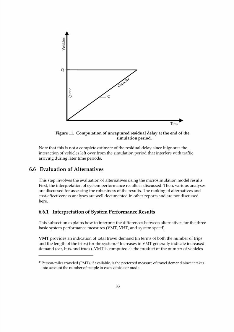
8/8/2019 Vol3 Guidelines
http://slidepdf.com/reader/full/vol3-guidelines 93/146
83
V e h i c l e s
Time
C
C a p a
c i t y
Q
Q u e u e
Figure 11. Computation of uncaptured residual delay at the end of thesimulation period.
Note that this is not a complete estimate of the residual delay since it ignores theinteraction of vehicles left over from the simulation period that interfere with trafficarriving during later time periods.
6.6 Evaluation of Alternatives
This step involves the evaluation of alternatives using the microsimulation model results.First, the interpretation of system performance results is discussed. Then, various analysesare discussed for assessing the robustness of the results. The ranking of alternatives andcost-effectiveness analyses are well documented in other reports and are not discussedhere.
6.6.1 Interpretation of System Performance Results
This subsection explains how to interpret the differences between alternatives for the threebasic system performance measures (VMT, VHT, and system speed).
VMT provides an indication of total travel demand (in terms of both the number of tripsand the length of the trips) for the system.13 Increases in VMT generally indicate increaseddemand (car, bus, and truck). VMT is computed as the product of the number of vehicles
13Person-miles traveled (PMT), if available, is the preferred measure of travel demand since it takesinto account the number of people in each vehicle or mode.
8/8/2019 Vol3 Guidelines
http://slidepdf.com/reader/full/vol3-guidelines 94/146
84
traversing a link and the length of the link, summed over all links. Since VMT is computedas a combination of the number of vehicles on the system and their length of travel, it canbe influenced both by changes in the number of vehicles and changes in the trip lengthsduring the simulation period. The following can cause changes in VMT between onealternative and the next:
• Random variations between one alternative and the next (use of the same randomnumber seed in both runs can reduce or eliminate the variation).
• Changed demand.
• Changed congestion causing vehicles to take different paths (increased congestionmay also reduce the number of vehicles that can complete their trip during thesimulation period, also decreasing VMT).
• Inability of the model to load the coded demand onto the network within the
simulation period (increased congestion may force the model to store some of thevehicle demand off-network because of bottlenecks at loading points; in this situation,increased congestion may actually lower VMT since stored vehicles cannot travel anydistance during the simulation period).
VHT provides an estimate of the amount of time expended traveling on the system.14 Decreases in VHT generally indicate improved system performance and reduced travelingcosts for the public. VHT is computed as the product of the link volume and the link traveltime, summed over all links. Since VHT is computed as a combination of the number ofvehicles and the time spent traveling, it can be influenced both by changes in demand (thenumber of vehicles) and changes in congestion (travel time). Changes in VHT betweenone alternative and the next can be caused by the following:
• Random variations between one alternative and the next.
• Changed demand.
• Changed congestion.
• Demand stored off-network because of excessive congestion at load points (increasedcongestion that causes demand to be stored off-network may reduce VHT if thesoftware does not accumulate delay for vehicles stored off-network).
Mean system speed is an indicator of overall system performance. Higher speedsgenerally indicate reduced travel costs for the public. The mean system speed is computedfrom the VMT and VHT as follows:
14Person-hours traveled (PHT), if available, provides a preferred measure of travel delay since ittakes into account the number of people delayed in each vehicle. This is especially important forcomparing the performance of HOV alternatives.
8/8/2019 Vol3 Guidelines
http://slidepdf.com/reader/full/vol3-guidelines 95/146
85
Mean System Speed = VMT /VHT (7)
Changes in the mean system speed between one alternative and the next can be caused bythe following:
• Random variations between one alternative and the next.
• Changed link speeds and delays caused by congestion.
• Changes in vehicle paths caused by congestion.
• Changes in vehicle demand.
• Changes in the number of vehicles stored off-network caused by excessive congestionat loading points.
Total system delay, if available, is useful because it reports the portion of total travel time
that is most irritating to the traveling public. However, defining “total system delay” canbe difficult. It depends on what the analyst or the software developer considers to be ideal(no delay) travel time. Some sources consider delay to include only the delay caused byincreases in demand above some base uncongested (free-flow) condition. Others add inthe base delay occurring at traffic control devices, even at low-flow conditions. Someinclude acceleration and deceleration delay. Others include only stopped delay. Theanalyst should consult the software documentation to ensure the appropriate use andinterpretation of this measurement of system performance.
6.6.2 Hypothesis Testing
When the microsimulation model is run several times for each alternative, the analyst mayfind that the variance in the results for each alternative is close to the difference in themean results for each alternative. How is the analyst to determine if the alternatives aresignificantly different? To what degree of confidence can the analyst claim that theobserved differences in the simulation results are caused by the differences in thealternatives and not just the result of using different random number seeds? This is thepurpose of statistical hypothesis testing. Hypothesis testing determines if the analyst hasperformed an adequate number of repetitions for each alternative to truly tell thealternatives apart at the analyst’s desired level of confidence. Hypothesis testing isdiscussed in more detail in appendix E.
6.6.3 Confidence Intervals and Sensitivity Analysis
Confidence intervals are a means of recognizing the inherent variation in microsimulationmodel results and conveying them to the decisionmaker in a manner that clearly indicatesthe reliability of the results. For example, a confidence interval would state that the meandelay for alternative x lies between 35.6 s and 43.2 s, with a 95-percent level of confidence.If the 95-percent confidence interval for alternative y overlaps that of x, the decisionmaker
8/8/2019 Vol3 Guidelines
http://slidepdf.com/reader/full/vol3-guidelines 96/146
86
would consider the results to be less favorable for either alternative. They could beidentical. Computation of the confidence interval is explained in appendix B.
A sensitivity analysis is a targeted assessment of the reliability of the microsimulationresults, given the uncertainty in the input or assumptions. The analyst identifies certain
input or assumptions about which there is some uncertainty and varies them to see whattheir impact might be on the microsimulation results.
Additional model runs are made with changes in demand levels and key parameters todetermine the robustness of the conclusions from the alternatives analysis. The analystmay vary the following:
• Demand.
• Street improvements assumed to be in place outside of the study area.
• Parameters for which the analyst has little information.
A sensitivity analysis of different demand levels is particularly valuable when evaluatingfuture conditions. Demand forecasts are generally less precise than the ability of themicrosimulation model to predict their impact on traffic operations. A 10-percent changein demand can cause a facility to go from 95 percent of capacity to 105 percent of capacity,with a concomitant massive change in the predicted delay and queuing for the facility.The analyst should estimate the confidence interval for the demand forecasts and test themicrosimulation at the high end of the confidence interval to determine if the alternativestill operates satisfactorily at the potentially higher demand levels.
The analyst should plan for some selected percentage above and below the forecasted
demand to allow for these uncertainties in future conditions. The analyst might considerat least a 10-percent margin of safety for the future demand forecasts. A larger rangemight be considered if the analyst has evidence to support the likelihood of greatervariances in the forecasts.
To protect against the possibility of both underestimates and overestimates in theforecasts, the analyst might perform two sensitivity tests—one with 110 percent of theinitial demand forecasts and the other with 90 percent of the initial demand forecasts—forestablishing a confidence interval for probable future conditions.15
Street improvements assumed to be in place outside the simulation study area can also
have a major impact on the simulation results by changing the amount of traffic that can
15Note that the percentage confidence interval (such as a 95 percent confidence interval) has notbeen stated here, so it cannot be claimed that there is a certain probability of the true value fallingwithin this 10 percent range. This is merely a sensitivity test of the impact of the demands being10 percent lower or 10 percent higher than that forecast, without knowing the likelihood of itactually happening.
8/8/2019 Vol3 Guidelines
http://slidepdf.com/reader/full/vol3-guidelines 97/146
87
enter or exit the facilities in the study area. Sensitivity testing would change the assumedfuture level of demand entering the study area and the assumed capacity of facilitiesleaving the study area to determine the impact of changes in the assumed streetimprovements.
The analyst may also run sensitivity tests to determine the effects of various assumptionsabout the parameter values used in the simulation. If the vehicle mix was estimated,variations in the percentage of trucks might be tested. The analyst might also test theeffects of different percentages of familiar drivers in the network.
6.6.4 Comparison of Results to the HCM
It is often valuable when explaining microsimulation model results to the general publicto report the results in terms of HCM levels of service. However, the analyst should bewell aware of the differences between the HCM and the microsimulation analysis whenmaking these comparisons.
Delay and Intersection Level of Service (LOS)
Delay is used in the HCM to estimate the LOS for signalized and unsignalizedintersections. There are distinctions in the ways microsimulation software and the HCMdefine delay and accumulate it for the purpose of assessing LOS.
The HCM bases its LOS grades for intersections on estimates of mean control delay for thehighest consecutive 15-min period within the hour. If microsimulation output is to beused to estimate LOS, then the results for each run must be accumulated over a similar 15-consecutive-minute time period and averaged over several runs with different random
number seeds to achieve a comparable result.
This still may not yield a fully comparable result, because all microsimulation modelsassign delay to the segment in which it occurs. For example, the delay associated with asingle approach to a traffic signal may be parceled out over several upstream links if thequeues extend beyond one link upstream from the intersection. Thus, when analysts seekto accumulate the delay at a signal, they should investigate whether the delay/queuesextend beyond the single approach links to the signal.
Finally, the HCM does not use total delay to measure signal LOS. It uses “control delay.” This is the component of total delay that results when a control signal causes a lane group
to reduce speed or to stop. It is measured by comparison with the uncontrolled condition.The analyst needs to review the software documentation and seek additionaldocumentation from the software vendor to understand how delay is computed by thesoftware.

8/8/2019 Vol3 Guidelines
http://slidepdf.com/reader/full/vol3-guidelines 98/146
88
Density and Freeway/Highway LOS
If microsimulation model reports of vehicle density are to be reported in terms of theirLOS implications, it is important to first translate the densities reported by the softwareinto the densities used by the HCM to report LOS for uninterrupted flow facilities.16
HCM 2000 defines freeway and highway LOS based on the average density of passengercar equivalent vehicles in a section of highway for the peak 15-min period within an hour.For ramp merge and diverge areas, only the density in the rightmost two lanes isconsidered for LOS. For all other situations, the density across all lanes is considered.Trucks and other heavy vehicles must be converted to passenger car equivalents using thevalues contained in the HCM according to vehicle type, facility type, section type, andgrade.
Queues
HCM 2000 defines a queue as: “A line of vehicles, bicycles, or persons waiting to be servedby the system in which the flow rate from the front of the queue determines the averagespeed within the queue. Slowly moving vehicles or people joining the rear of the queueare usually considered part of the queue.” These definitions are not implementable withina microsimulation environment since “waiting to be served” and “slowly” are not easilydefined. Consequently, alternative definitions based on maximum speed, acceleration,and proximity to other vehicles have been developed for use in microsimulation.
Note also that for most microsimulation programs, the number of queued vehiclescounted as being in a particular turn-pocket lane or through lane cannot exceed the storagecapacity of that lane. Any overflow is reported for the upstream lane and link where itoccurs, not the downstream cause of the queue. Unlike macroscopic approaches that
assign the entire queue to the bottleneck that causes it, microsimulation models can onlyobserve the presence of a queue; they currently do not assign a cause to it. So, to obtain the95-percent queue length, it may be necessary to temporarily increase the length of thestorage area so that all queues are appropriately tallied in the printed output.
6.7 Example Problem: Alternatives Analysis
The same example problem from the previous chapters is continued here. The task now isto apply the calibrated model to the analysis of the ramp metering project and itsalternatives.
Step 1: Baseline Demand Forecast
A 5-year forecast was estimated using a straight-line growth approach assuming 2 percentgrowth per year uncompounded. The result was a forecasted 10-percent increase in traffic
16Note that density is NOT used as an LOS measurement for interrupted flow facilities, such as citystreets with signals and intersections with stop signs.

8/8/2019 Vol3 Guidelines
http://slidepdf.com/reader/full/vol3-guidelines 99/146
89
demand for the corridor. The forecasted growth for individual links and ramps variedfrom this average value.
Since the existing conditions were uncongested and the growth forecast is a modest10 percent growth, the forecasted demand was not constrained because of anticipated
capacity constraints on the entry links to the corridor.
Since a 5-year forecast is being performed, it was considered to be fairly reliable for such ashort time period. No extra allowance was added to the forecasts or subtracted from themto account for uncertainty in the demand forecasts.
Step 2: Generation of Alternatives
Two alternatives will be tested with the calibrated model—no-build and build. The buildalternative consists of ramp metering on the two eastbound freeway on-ramps. The no-build alternative has no ramp metering. Figure 12 below illustrates the coding of one ofthe ramp meters.
Figure 12. Ramp meter geometry.
Step 3: Selection of MOEs
The following system MOEs were selected for evaluation of the alternatives: VMT, VHT,and delay (vehicle-hours). The selected indicator of localized problems was a “blockedlink,” indicating that the queue filled up and overflowed the available storage in the link.

8/8/2019 Vol3 Guidelines
http://slidepdf.com/reader/full/vol3-guidelines 100/146
90
It was opted to report the mean results rather than the 95-percent worst case results.
Step 4: Model Application
The model was run 10 times for each alternative. The results were output into a
spreadsheet and averaged for each alternative.
The impact of ramp meters on route choice was estimated outside of the model using aregional travel demand model to predict the amount of diversion. The regional modelpredicted that diversion was implemented in the simulation model by manually adjustingthe turn percentages at the appropriate upstream intersections and ramp junctions.
The initialization period was automatically excluded from the tabulated results by theselected software program.
The results were reviewed to determine if building queues17 were extending beyond thephysical boundaries of the model or the temporal boundaries of the analytical period.None was found, so it was not necessary to correct the model results for untabulatedcongestion.
Because of the modest differences in congestion between the alternatives, induceddemand was not considered to be a significant factor in this analysis. No adjustmentswere made to the baseline demand forecasts.
Signal/meter control optimization was performed outside of the model using macroscopicsignal optimization software and ramp meter optimization software. The recommendedoptimal settings were input into the simulation model. Separate optimizations wereperformed for the no-build and build alternatives.
Step 5: Tabulation of Results
The model results for 10 repetitions of each alternative were output into a spreadsheet andaveraged for each alternative (see table 7 below). A review of the animation outputindicated that post-model corrections of untallied congestion were not necessary.18
17Recurrent queues at signals that occur during each cycle are not considered to be building queuesindicative of unserved demand that might bias the results for an alternative.
18No increasing queues indicating underserved demand were found.
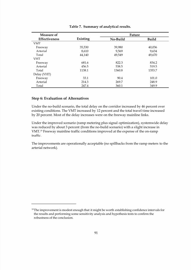
8/8/2019 Vol3 Guidelines
http://slidepdf.com/reader/full/vol3-guidelines 101/146
91
Table 7. Summary of analytical results.
FutureMeasure ofEffectiveness Existing No-Build Build
VMT
Freeway 35,530 39,980 40,036Arterial 8,610 9,569 9,634Total 44,140 49,549 49,670
VHTFreeway 681.6 822.3 834.2Arterial 456.5 538.5 519.5Total 1138.1 1360.8 1353.7
Delay (VHT)Freeway 33.1 90.4 101.0Arterial 214.3 269.7 248.9Total 247.4 360.1 349.9
Step 6: Evaluation of Alternatives
Under the no-build scenario, the total delay on the corridor increased by 46 percent overexisting conditions. The VMT increased by 12 percent and the total travel time increasedby 20 percent. Most of the delay increases were on the freeway mainline links.
Under the improved scenario (ramp metering plus signal optimization), systemwide delaywas reduced by about 3 percent (from the no-build scenario) with a slight increase inVMT.19 Freeway mainline traffic conditions improved at the expense of the on-ramptraffic.
The improvements are operationally acceptable (no spillbacks from the ramp meters to thearterial network).
19The improvement is modest enough that it might be worth establishing confidence intervals forthe results and performing some sensitivity analysis and hypothesis tests to confirm therobustness of the conclusion.

8/8/2019 Vol3 Guidelines
http://slidepdf.com/reader/full/vol3-guidelines 102/146
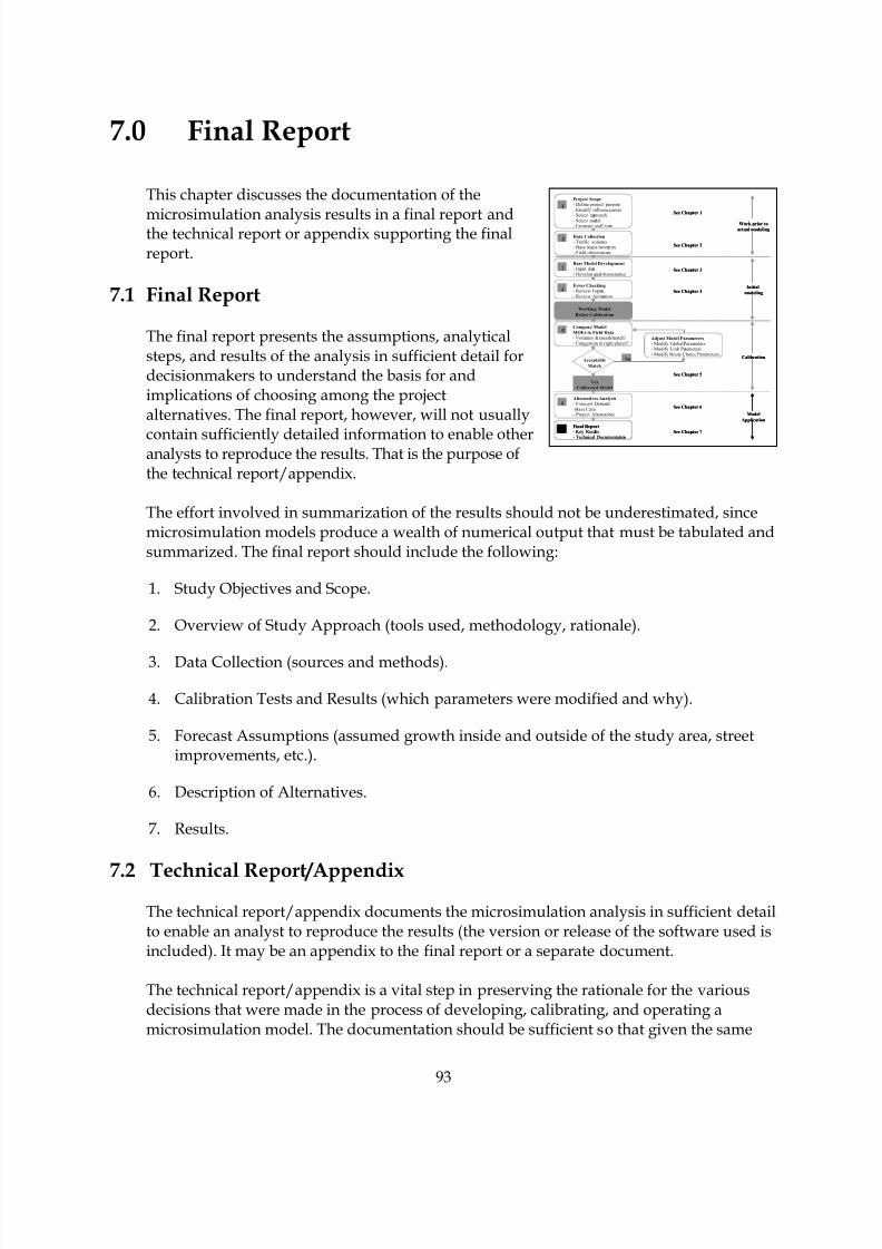
8/8/2019 Vol3 Guidelines
http://slidepdf.com/reader/full/vol3-guidelines 103/146
93
No
Data Collection
- Traffic volumes- Base maps/inventory- Field observations
2
1
Project Scope
- Define project purpose- Identify influence areas- Select approach- Select model- Estimate staff time
See Chapter 1
See Chapter 2
See Chapter 3
See Chapter 4
Work prior to
actual modeling
Initial
modeling
Yes
Calibrated Model
See Chapter 5
Calibration
See Chapter 6
See Chapter 7
Model
Application
Base Model Development
- Input data- Develop qualityassurance
3
Error Checking
- Review Inputs- Review Animation
4
Compare Model
MOEs to Field Data
- Volumes & speedsmatch?- Congestion in right places?
5
Alternatives Analysis
- Forecast Demand-Base Case- Project Alternatives
6
Final Report
- Key Results
- Technical Documentation
7
Working Model
Before Calibration
Acceptable
Match
Adjust Model Parameters
- Modify Global Parameters- Modify Link Parameters- Modify Route Choice Parameters
7.0 Final Report
This chapter discusses the documentation of the
microsimulation analysis results in a final report andthe technical report or appendix supporting the finalreport.
7.1 Final Report
The final report presents the assumptions, analyticalsteps, and results of the analysis in sufficient detail fordecisionmakers to understand the basis for andimplications of choosing among the projectalternatives. The final report, however, will not usually
contain sufficiently detailed information to enable otheranalysts to reproduce the results. That is the purpose ofthe technical report/appendix.
The effort involved in summarization of the results should not be underestimated, sincemicrosimulation models produce a wealth of numerical output that must be tabulated andsummarized. The final report should include the following:
1. Study Objectives and Scope.
2. Overview of Study Approach (tools used, methodology, rationale).
3. Data Collection (sources and methods).
4. Calibration Tests and Results (which parameters were modified and why).
5. Forecast Assumptions (assumed growth inside and outside of the study area, streetimprovements, etc.).
6. Description of Alternatives.
7. Results.
7.2 Technical Report/Appendix
The technical report/appendix documents the microsimulation analysis in sufficient detailto enable an analyst to reproduce the results (the version or release of the software used isincluded). It may be an appendix to the final report or a separate document.
The technical report/appendix is a vital step in preserving the rationale for the variousdecisions that were made in the process of developing, calibrating, and operating amicrosimulation model. The documentation should be sufficient so that given the same

8/8/2019 Vol3 Guidelines
http://slidepdf.com/reader/full/vol3-guidelines 104/146
94
input files, another analyst can understand the calibration process and repeat thealternatives analysis.
The technical report/appendix should include the model input and output files (inelectronic format) for the final model calibration run and alternatives analysis model runs.
In addition to a diskette with the calibration and alternatives analysis files (input andoutput), the technical report/appendix should include a printed listing of the files on thediskette with a text description of the contents and purpose of each file.
8/8/2019 Vol3 Guidelines
http://slidepdf.com/reader/full/vol3-guidelines 105/146
95
Appendix A: Traffic MicrosimulationFundamentals
This section provides an overview of the technical aspects of microsimulation. It identifiesand defines the terminology typically used, and what model types and procedures aregenerally employed in microsimulation. This section also provides a general introductionto traffic simulation models. Readers interested in additional details on the technicalaspects of microsimulation may consult the Revised Monograph on Traffic Flow Theory(Chapter 10: Traffic Simulation) or other documents.
A.1 Overview
Simulation models are designed to emulate the behavior of traffic in a transportation
network over time and space to predict system performance. Simulation models includethe mathematical and logical abstractions of real-world systems implemented in computersoftware. Simulation model runs can be viewed as experiments performed in thelaboratory rather than in the field.
A.2 System Update Mechanism
Traffic simulation models describe the changes in the system state through discreteintervals in time. There are generally two types of models, depending on whether theupdate time intervals are fixed or variable:
Discrete Time (Time-Scan) Models: The system is being updated at fixed-time intervals.For example, the model calculates the vehicle position, speed, and acceleration at 1-sintervals. The choice of the update time interval depends on how accurately the systemneeds to be simulated at the expense of computer-processing time. Most microsimulationmodels employ a 0.1-s resolution for updating the system. Traffic systems are typicallymodeled using time-scan models because they experience a continuous change in state.
Discrete Event (Event-Scan) Models: In these models, the time intervals vary in lengthand correspond to the intervals between events. For example, a pre-timed traffic signalindication (e.g., green) remains constant for 30 s until its state changes instantaneously toyellow. The operation of the signal is described by recording its changes in state whenevents occur, rather than monitoring the state of the signal each second. Event-scanningmodels typically achieve significant reductions in computer run time. However, they aresuitable for simulating systems whose states change infrequently.

8/8/2019 Vol3 Guidelines
http://slidepdf.com/reader/full/vol3-guidelines 106/146
96
A.3 Traffic Stream Representation
Simulation models are typically classified according to the level of detail at which theyrepresent the traffic stream. These include:
Microscopic Models: These models simulate the characteristics and interactions ofindividual vehicles. They essentially produce trajectories of vehicles as they movethrough the network. The processing logic includes algorithms and rules describing howvehicles move and interact, including acceleration, deceleration, lane changing, andpassing maneuvers.
Mesoscopic Models: These models simulate individual vehicles, but describe theiractivities and interactions based on aggregate (macroscopic) relationships. Typicalapplications of mesoscopic models are evaluations of traveler information systems. Forexample, they can simulate the routing of individual vehicles equipped with in-vehicle,real-time travel information systems. The travel times are determined from the simulated
average speeds on the network links. The average speeds are, in turn, calculated from aspeed-flow relationship.
Macroscopic Models: These models simulate traffic flow, taking into considerationaggregate traffic stream characteristics (speed, flow, and density) and their relationships.Typically, macroscopic models employ equations on the conservation of flow and on howtraffic disturbances (shockwaves) propagate in the system. They can be used to predictthe spatial and temporal extent of congestion caused by traffic demand or incidents in anetwork; however, they cannot model the interactions of vehicles on alternative designconfigurations.
Microscopic models are potentially more accurate than macroscopic simulation models.However, they employ many more parameters that require calibration. Also, theparameters of the macroscopic models (e.g., capacity) are observable in the field. Most ofthe parameters of the microscopic models cannot be observed directly in the field (e.g.,minimum distances between vehicles in car-following situations).
A.4 Randomness in Traffic Flow
Simulation models are also classified by how they represent the randomness in the trafficflow, including:
Deterministic Models: These models assume that there is no variability in the driver-vehicle characteristics. For example, it is assumed that all drivers have a critical gap of 5 sin which to merge into a traffic stream, or all passenger cars have a vehicle length of 4.9 m(16 ft).
Stochastic Models: These models assign driver-vehicle characteristics from statisticaldistributions using random numbers. For example, the desired speed of a vehicle israndomly generated from an assumed normal distribution of desired speeds, with a meanof 105 km/h (65 mi/h) and a standard deviation of 8 km/h (5 mi/h). Stochastic
8/8/2019 Vol3 Guidelines
http://slidepdf.com/reader/full/vol3-guidelines 107/146
97
simulation models have routines that generate random numbers. The sequence of randomnumbers generated depends on the particular method and the initial value of the randomnumber (random number seed). Changing the random number seed produces a differentsequence of random numbers, which, in turn, produces different values of driver-vehiclecharacteristics.
Stochastic models require additional parameters to be specified (e.g., the form andparameters of the statistical distributions that represent the particular vehiclecharacteristic). More importantly, the analysis of the simulation output should considerthat the results from each model run vary with the input random number seed forotherwise identical input data. Deterministic models, in contrast, will always produce thesame results with identical input data.
A.5 Microsimulation Process
Microsimulation models employ several submodels, analytical relationships, and logic to
model traffic flow. Detailed descriptions of each submodel are beyond the scope of thissection. Instead, this document focuses on some key aspects of the simulation process thatwill probably affect the choice of the particular tool to be used and the accuracy of theresults.
Simulation models include algorithms and logic to:
• Generate vehicles into the system to be simulated.
• Move vehicles into the system.
• Model vehicle interactions.
A.5.1 Vehicle Generation
Generating Vehicles Into the Traffic Stream
At the beginning of the simulation run, the system is empty. Vehicles are generated at theentry nodes of the analytical network, based on the input volumes and an assumedheadway distribution. Suppose that the specified volume is V = 600 veh/h for a 15-minanalytical period and that the model uses a uniform distribution of vehicle headways.Then, a vehicle will be generated at time intervals:
H = mean headway = 3600/V = 3600/600 = 6 s (8)
If the model uses the shifted negative exponential distribution to simulate the arrival ofvehicles at the network entry node instead of the uniform distribution, then vehicles willbe generated as time intervals:
h- H + R)]-(1 [- )h-(H =h minmin ln (9)

8/8/2019 Vol3 Guidelines
http://slidepdf.com/reader/full/vol3-guidelines 108/146
98
where:
h = headway (in seconds) separating each generated vehicle
hmin = specified minimum headway (e.g., 1.0 s)
R = random number (0 to 1.0)
Generating Driver-Vehicle Attributes
When a vehicle is generated at the entry of the network, the simulation model assignsdriver-vehicle characteristics. The following characteristics or attributes are commonlygenerated for each driver-vehicle unit:
Vehicle: Type (car, bus, truck), length, width, maximum acceleration and deceleration,maximum speed, maximum turn radius, etc.
Driver: Driver aggressiveness, reaction time, desired speed, critical gaps (for lanechanging, merging, crossing), destination (route), etc.
Note that the different models may employ additional attributes for each driver-vehicleunit to ensure that the model replicates real-world conditions. Each attribute may berepresented in the model by constants (e.g., all passenger cars have a vehicle length of 4.9m (16 ft)), functional relationships (e.g., maximum vehicle acceleration is a linear functionof its current speed), or probability distributions (e.g., driver’s desired speed is obtainedfrom a normal distribution). Most microsimulation models employ statistical distributionsto represent the driver-vehicle attributes. The statistical distributions employed torepresent the variability of the driver-vehicle attributes and their parameters must becalibrated to reflect local conditions.
Figure 13 illustrates a generic process for generating driver-vehicle attributes for astochastic microscopic simulation model. Drivers are randomly assigned an“aggressiveness index” ranging from 1 (very aggressive) to 10 (very cautious), drawn froma uniform distribution to represent the range of human behavior. Once the value of theaggressiveness has been assigned (X = 7 in this example), it is used to assign the value ofthe free-flow speed (97 km/h) and the acceptable deceleration (-3.4 m/s2 (-11 ft/s2)) fromthe corresponding distribution of speeds and accelerations.
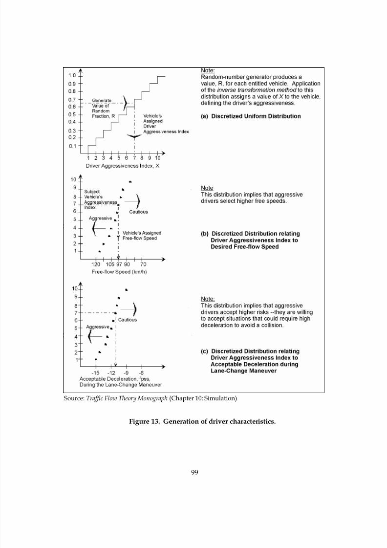
8/8/2019 Vol3 Guidelines
http://slidepdf.com/reader/full/vol3-guidelines 109/146
99
Source: Traffic Flow Theory Monograph (Chapter 10: Simulation)
Figure 13. Generation of driver characteristics.
8/8/2019 Vol3 Guidelines
http://slidepdf.com/reader/full/vol3-guidelines 110/146
8/8/2019 Vol3 Guidelines
http://slidepdf.com/reader/full/vol3-guidelines 111/146
101
Car Following
The interaction between a leader and follower pair of vehicles traveling in the same lane,is generally assumed to be a form of stimulus-response mechanism:
Response follower (t+T ) = (sensitivity) • (stimulus) t (10)
where:
T = reaction time (time lag) for the response of the following vehicle
Car-following models for highway traffic were proposed since the inception of the traffic-flow theory in the early 1950s. Extensive experimentation and theoretical work wereperformed at the General Motors (GM) laboratories and elsewhere. Most of the existingsimulation models employ fail-safe car-following algorithms. Such algorithms simulatecar-following behavior by maintaining a minimum safe distance between vehicles subject
to stochastically generated vehicle characteristics (e.g., maximum acceleration anddeceleration rates). The fail-safe car-following algorithms currently implemented in mostsimulation models consist of the following components:
1. An equation that calculates the acceleration (deceleration) of the following vehicle inresponse to the motion of its leader to maintain a target headway (spacing), dependingon the driver-vehicle characteristics.
) X ,T , s,v,v( F =a i f l f (11)
where:
a f = acceleration of the following vehicle after a reaction time T
vl and vf = speeds of the leading and following vehicles, respectively
s = distance between vehicles
X i = parameters specific to the particular car-following model
2. The computed acceleration rate above must not exceed the maximum acceleration ratefor the specific vehicle type and must not result in a higher speed than the vehicle’sdesired speed.
3. Furthermore, the computed acceleration of the follower above must satisfy the “safe-
following” rule (i.e., the follower should always maintain a minimum separation fromthe leader). If the value of the safe-following acceleration is smaller then the car-following acceleration computed above, the former is implemented.

8/8/2019 Vol3 Guidelines
http://slidepdf.com/reader/full/vol3-guidelines 112/146
102
Lane Changing
The modeling of lane changing is based on the gap-acceptance process. A vehicle maychange lanes if the available gap in the target lane is greater than its critical gap. Typically,three types of lane changes are modeled:
1. A mandatory lane change occurs when a vehicle is required to exit the current lane.Merging from an on-ramp onto the freeway is an example of a mandatory lanechange. A vehicle must execute a lane change under several circumstances:
a. Current lane is ending (lane drop)
b. Must move to the outer lane(s) to exit the freeway via an off-ramp
c. Current lane will not accommodate its movement or vehicle type (e.g., HOV lane)
d. Lane is blocked because of incidents or other events
2. A discretionary lane change occurs when a vehicle changes lanes to improve itsposition (i.e., travel at the desired speed). If a driver is impeded in the current lanebecause of a slower moving vehicle in front, he or she may consider changing lanes toimprove his or her position (i.e., resume his or her desired speed). The lane-changinglogic determines which of the adjacent lanes (if more than one is available) is the bestcandidate. To be a candidate, the lane’s channelization must accommodate the subjectvehicle, be free of blockage, and not end close by. Lane changing is performed subjectto the availability of gaps in the candidate lane and the acceptability of the gaps by thesubject vehicle.
On a surface-street network, discretionary lane changes may occur because of various
impedance factors perceived by the driver, including:
a. Queue length at the stop line.
b. Heavy truck traffic.
c. Bus transit operations.
d. Turning movements from shared lanes.
e. Pedestrian interference with turning vehicles.
f. Parking activities.
3. An anticipatory lane change occurs when a vehicle may change lanes in anticipation
of slowdowns in its current lane further downstream as a result of merging orweaving. The decision to change lanes is based on the difference in speed at thelocation of the merge or weave, between the vehicles in the current lane and theadjacent lane not directly involved in the merge or weave. The lane-changing logicrecognizes that a driver may accelerate or decelerate to create acceptable gaps to changelanes. Consider a vehicle A that desires to merge into a gap between vehicles B and C (Bcurrently is the leader of C). Vehicle A will accept the gap if the time headway betweenit and vehicle B is greater than some critical value g(A,B) and the time headway

8/8/2019 Vol3 Guidelines
http://slidepdf.com/reader/full/vol3-guidelines 113/146
103
between it and vehicle C is greater than some critical value g(A,C). However, the criticaltime headway values are not constant, but are dependent on the followingconsiderations:
• Critical time headways depend on vehicle speeds. Vehicle A will accept a smaller
critical headway if it is going slower than vehicle B.
• Lane changing takes place over a finite period of time. During this time period, thedriver who is changing lanes can adjust his or her position with respect to the newleader by decelerating.
• The new follower may cooperate with the driver who is changing lanes bydecelerating to increase the size of the gap.
These considerations are typically combined in a risk measure. More aggressive driverswould accept a higher risk value (i.e., shorter gaps and higher acceleration/
deceleration rates) to change lanes. Moreover, the risk value may be further increased,depending on the type of lane change and the situation. For example, a mergingvehicle reaching the end of the acceleration lane may accept much higher risk values(forced lane changes).
The model’s lane-changing logic and parameters have important implications for trafficperformance, especially for freeway merging and weaving areas. In addition, the timeassumed for completion of the lane-change maneuver affects traffic performance becausethe vehicle occupies both lanes (original and target lanes) during this time interval.Furthermore, one lane change is allowed per simulation time interval.

8/8/2019 Vol3 Guidelines
http://slidepdf.com/reader/full/vol3-guidelines 114/146
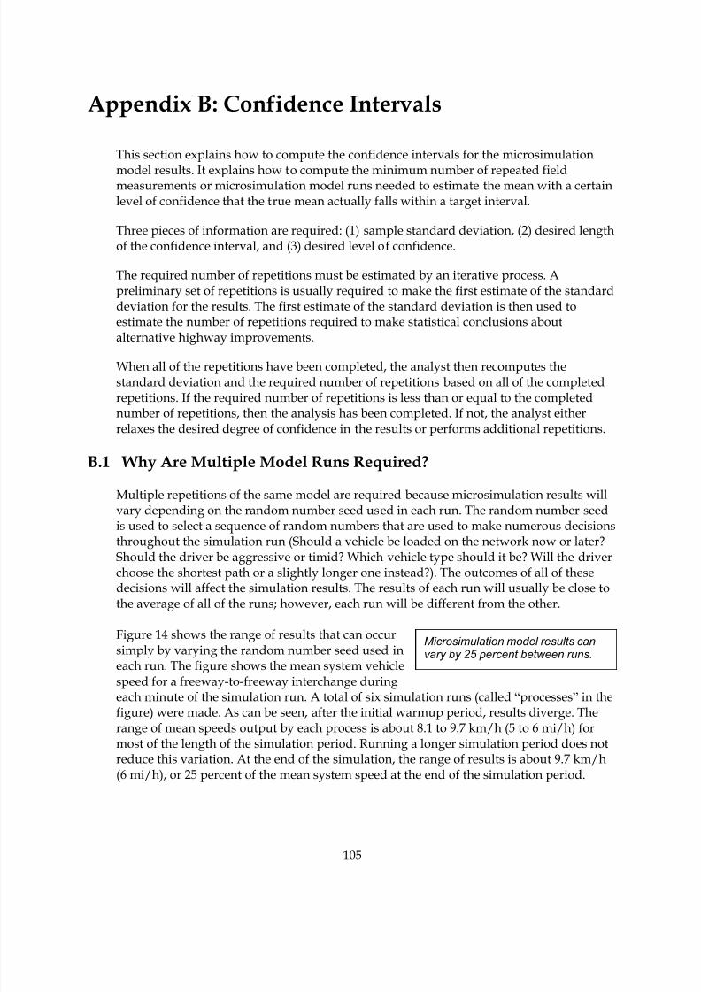
8/8/2019 Vol3 Guidelines
http://slidepdf.com/reader/full/vol3-guidelines 115/146
105
Appendix B: Confidence Intervals
This section explains how to compute the confidence intervals for the microsimulation
model results. It explains how to compute the minimum number of repeated fieldmeasurements or microsimulation model runs needed to estimate the mean with a certainlevel of confidence that the true mean actually falls within a target interval.
Three pieces of information are required: (1) sample standard deviation, (2) desired lengthof the confidence interval, and (3) desired level of confidence.
The required number of repetitions must be estimated by an iterative process. Apreliminary set of repetitions is usually required to make the first estimate of the standarddeviation for the results. The first estimate of the standard deviation is then used toestimate the number of repetitions required to make statistical conclusions aboutalternative highway improvements.
When all of the repetitions have been completed, the analyst then recomputes thestandard deviation and the required number of repetitions based on all of the completedrepetitions. If the required number of repetitions is less than or equal to the completednumber of repetitions, then the analysis has been completed. If not, the analyst eitherrelaxes the desired degree of confidence in the results or performs additional repetitions.
B.1 Why Are Multiple Model Runs Required?
Multiple repetitions of the same model are required because microsimulation results willvary depending on the random number seed used in each run. The random number seed
is used to select a sequence of random numbers that are used to make numerous decisionsthroughout the simulation run (Should a vehicle be loaded on the network now or later?Should the driver be aggressive or timid? Which vehicle type should it be? Will the driverchoose the shortest path or a slightly longer one instead?). The outcomes of all of thesedecisions will affect the simulation results. The results of each run will usually be close tothe average of all of the runs; however, each run will be different from the other.
Figure 14 shows the range of results that can occursimply by varying the random number seed used ineach run. The figure shows the mean system vehiclespeed for a freeway-to-freeway interchange during
each minute of the simulation run. A total of six simulation runs (called “processes” in thefigure) were made. As can be seen, after the initial warmup period, results diverge. Therange of mean speeds output by each process is about 8.1 to 9.7 km/h (5 to 6 mi/h) formost of the length of the simulation period. Running a longer simulation period does notreduce this variation. At the end of the simulation, the range of results is about 9.7 km/h(6 mi/h), or 25 percent of the mean system speed at the end of the simulation period.
Microsimulation model results canvary by 25 percent between runs.
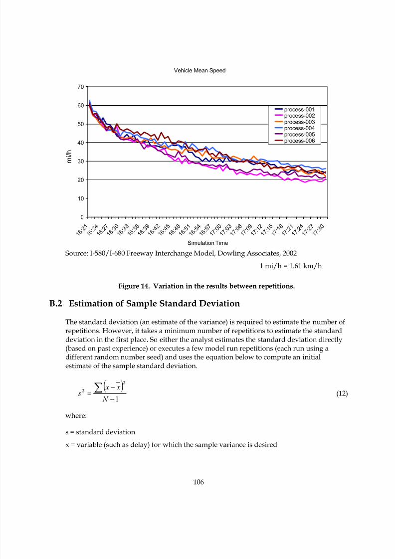
8/8/2019 Vol3 Guidelines
http://slidepdf.com/reader/full/vol3-guidelines 116/146
106
Vehicle Mean Speed
0
10
20
30
40
50
60
70
1 6 : 2 1
1 6 : 2 4
1 6 : 2 7
1 6 : 3 0
1 6 : 3 3
1 6 : 3 6
1 6 : 3 9
1 6 : 4 2
1 6 : 4 5
1 6 : 4 8
1 6 : 5 1
1 6 : 5 4
1 6 : 5 7
1 7 : 0 0
1 7 : 0 3
1 7 : 0 6
1 7 : 0 9
1 7 : 1 2
1 7 : 1 5
1 7 : 1 8
1 7 : 2 1
1 7 : 2 4
1 7 : 2 7
1 7 : 3 0
Simulation Time
m p h
process-001process-002process-003process-004process-005process-006
Source: I-580/I-680 Freeway Interchange Model, Dowling Associates, 2002
1 mi/h = 1.61 km/h
Figure 14. Variation in the results between repetitions.
B.2 Estimation of Sample Standard Deviation
The standard deviation (an estimate of the variance) is required to estimate the number ofrepetitions. However, it takes a minimum number of repetitions to estimate the standarddeviation in the first place. So either the analyst estimates the standard deviation directly(based on past experience) or executes a few model run repetitions (each run using adifferent random number seed) and uses the equation below to compute an initialestimate of the sample standard deviation.
( )1
2
2
−
−= ∑ N
x x s (12)
where:
s = standard deviation
x = variable (such as delay) for which the sample variance is desired
m i / h
8/8/2019 Vol3 Guidelines
http://slidepdf.com/reader/full/vol3-guidelines 117/146
107
x = average value of the variable produced by the model runs
N = number of model runs
Unless the analyst already knows the standard deviation from experience, it is
recommended that four repetitions be performed for the initial estimation of the standarddeviation. This initial estimate is then revisited and revised later if and when additionalrepetitions are performed for the purposes of obtaining more precise estimates of meanvalues or for alternatives analysis.
B.3 Selection of Desired Confidence Level
The confidence level is the probability that the true mean lies within the target confidenceinterval. The analyst must decide to what degree he or she wishes to know the interval inwhich the true mean value lies. The usual approach is to pick a 95-percent level ofconfidence; however, analysts may choose higher or lower levels of confidence. Higher
levels of confidence require more repetitions.
B.4 Selection of Desired Confidence Interval
The confidence interval is the range of values within which the true mean value may lie.The length of the interval is at the discretion of the analyst and may vary according to thepurposes for which the results will be used. For example, if the analyst is testingalternatives that are very similar, then a very small confidence interval will be desirable todistinguish between the alternatives. If the analyst is testing alternatives with greaterdifferences, then a larger confidence interval can be tolerated. Smaller confidence intervalsrequire more repetitions to achieve a given level of confidence. Confidence intervals that
are less than half the value of the standard deviation will require a large number ofrepetitions to achieve reasonable confidence levels.20
B.4.1 Computation of Minimum Repetitions
It is impossible to know in advance exactly how many model runs will be needed todetermine a mean (or any other statistical value) to the analyst’s satisfaction. However,after a few model runs, the analyst can make an estimate of how many more runs may berequired to obtain a statistically valid result.
The required minimum number of model repetitions is computed using the following
equation:
N
st CI N 1),2/1(%1 2 −−− ∗=
α α (13)
20With such a tight confidence interval, the analyst may be striving for a degree of precision notreflected under real-world conditions.

8/8/2019 Vol3 Guidelines
http://slidepdf.com/reader/full/vol3-guidelines 118/146
108
where:
CI(1-alpha)% = (1-alpha)% confidence interval for the true mean, where alpha equals theprobability of the true mean not lying within the confidence interval
t(1-alpha/2),N-1 = Student’s t-statistic for the probability of a two-sided error summing to alphawith N-1 degrees of freedom, where N equals the number of repetitions
s = standard deviation of the model results
Note that when solving this equation for N, it will be necessary to iterate until theestimated number of repetitions matches the number of repetitions assumed whenlooking up the t statistic. Table 8 shows the solutions to the above equation in terms of theminimum number of repetitions for various desired confidence intervals and desireddegrees of confidence.
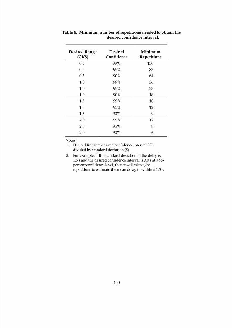
8/8/2019 Vol3 Guidelines
http://slidepdf.com/reader/full/vol3-guidelines 119/146

8/8/2019 Vol3 Guidelines
http://slidepdf.com/reader/full/vol3-guidelines 120/146

8/8/2019 Vol3 Guidelines
http://slidepdf.com/reader/full/vol3-guidelines 121/146
111
Appendix C: Estimation of the SimulationInitialization Period
Simulation model runs usually start with zero vehicles on the network. If the simulationoutput is being compared to field measurements (as in calibration), then the artificialperiod where the simulation model starts out with zero vehicles (the warmup period)must be excluded from the reported statistics for system performance. Some softwareprograms will do this automatically. For others, the warmup period must be computedoffline by the analyst. This section explains how to identify the warmup period.
The number of vehicles present at any one time on the network is used to determinewhether the model has reached equilibrium and, therefore, can start tallying performancestatistics for the network. Once the number of vehicles present on the network ceases toincrease by a minimum specified amount, then the warmup period is deemed to have
been concluded (see figure 15).
If the number of vehicles and the mean speed do not level off within the first 15 min, itcould be that the demand coded by the analyst for the system is greater than the systemcapacity. In this case, congestion will never level off. This will result in less accuratecongestion statistics since the system never clears the congestion. The analyst shouldconsider extending the starting and end times of the simulation to incorporate lowerdemand periods before and after the peak period.
If it is not feasible to extend the simulation period to uncongested time periods, theanalyst should choose a warmup period that is equal to at least twice the estimated travel
time at free-flow conditions to traverse the length of the network. For example, if thefreeway being modeled is 8.1 km (5 mi) long, it takes roughly 5 min to traverse its lengthat the free-flow speed, so the warmup period is set at 10 min.
Note that in this example, the number of vehicles in the system is generally steadilyincreasing. The system never reaches equilibrium. Initialization is achieved when thenumber of vehicles entering the system is approximately equal to the number leaving thesystem (even though this slight decline is later superceded by greater increases). Thegenerally increasing trend in the number of vehicles present in the system suggests thatthe simulation period should be extended earlier and later to incorporate lower demandperiods at the beginning and the end of the peak period.
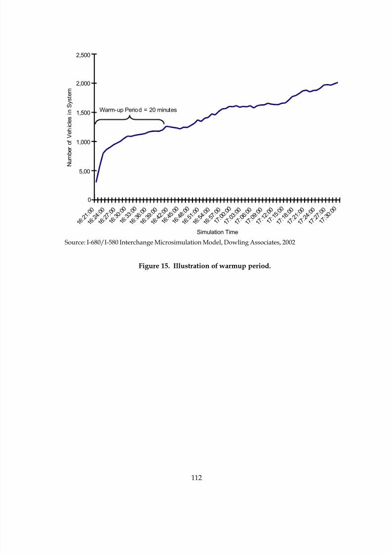
8/8/2019 Vol3 Guidelines
http://slidepdf.com/reader/full/vol3-guidelines 122/146
112
0
5,00
1,000
1,500
2,000
2,500
1 6 : 2 1 : 0 0
1 6 : 2 4 : 0 0
1 6 : 2 7 : 0 0
1 6 : 3 0 : 0 0
1 6 : 3 3 : 0 0
1 6 : 3 6 : 0 0
1 6 : 3 9 : 0 0
1 6 : 4 2 : 0 0
1 6 : 4 5 : 0 0
1 6 : 4 8 : 0 0
1 6 : 5 1 : 0 0
1 6 : 5 4 : 0 0
1 6 : 5 7 : 0 0
1 7 : 0 0 : 0 0
1 7 : 0 3 : 0 0
1 7 : 0 6 : 0 0
1 7 : 0 9 : 0 0
1 7 : 1 2 : 0 0
1 7 : 1 5 : 0 0
1 7 : 1 8 : 0 0
1 7 : 2 1 : 0 0
1 7 : 2 4 : 0 0
1 7 : 2 7 : 0 0
1 7 : 3 0 : 0 0
Simulation Time
N u m b e r o f V e h i c l e s i n S y s t e m
Warm-up Period = 20 minutes
Source: I-680/I-580 Interchange Microsimulation Model, Dowling Associates, 2002
Figure 15. Illustration of warmup period.

8/8/2019 Vol3 Guidelines
http://slidepdf.com/reader/full/vol3-guidelines 123/146
113
Appendix D: Simple Search Algorithms forCalibration
Since simulation models are complex, it is not typically possible to formulate the modelsas a closed-form equation for which traditional calculus techniques can be applied to finda minimum value solution. It is necessary to use some sort of search algorithm that relieson multiple operations of the simulation model, plotting of the output results as points,and searching between these points for the optimal solution. Search algorithms arerequired to find the optimal solution to the calibration problem. The calibration problem isa nonlinear least-squares optimization problem.
There are many software programs available for identifying the optimal combination ofcalibration parameters for minimizing the squared error between the field observationsand the simulation model. The Argonne National Laboratory (www-fp.mcs.anl.gov/
otc/Guide/SoftwareGuide/Categories/nonlinleastsq.html) lists several softwareprograms for nonlinear least-squares parameter estimation.
The sections below illustrate some simple approaches available for single-parameterestimation and dual-parameter estimation when working with a stand-alone simulationmodel. Estimation of three or more parameters, however, would require the use of asoftware program.
D.1 Single-Parameter Search Algorithm (Golden Section)1
Several methods are available for finding the value of a single parameter that minimizes
the squared error between the model and the observations. These methods include Newton ’sMethod, Secant Method, Quadratic Approximation Methods, and the Golden SectionMethod. The Golden Section Method is illustrated in the example below.
D.1.1 Example of Golden Section Method
Objective: Find the global value of the mean headway between vehicles that minimizesthe squared error between the field counts of traffic volumes and the model estimates.
Approach: Use the Golden Section Method to identify the optimal mean headway.
1 References: Hillier, F.S., and G.J. Lieberman, Introduction to Operations Research, Sixth Edition,McGraw-Hill, New York, 1995; Taha, H.A., Operations Research, An Introduction, Seventh Edition,Prentice-Hall, New York, 2003 (if the seventh edition is not available, look for the sixth editionpublished in 1996).

8/8/2019 Vol3 Guidelines
http://slidepdf.com/reader/full/vol3-guidelines 124/146
114
Step 1: Identify the maximum and minimum acceptable values for the parameterto be optimized.
This step brackets the possible range of the parameter in which the optimal solution ispresumed to lie. The user can select the appropriate range. For this example, we will set
the minimum acceptable value for the mean headway at 0.5 s and the maximum at 2.0 s.The larger the range, the more robust the search. However, it will take longer to find theoptimum value. The smaller the range of acceptable values, the greater the likelihood thatthe best solution lies outside of the range.
Step 2: Compute the squared error for maximum and minimum values.
The simulation model is run to determine the volumes predicted when the maximumacceptable mean headway is input and again for the minimum acceptable headway. Eitherrandomization should be turned off or the model should be run several times with eachmean headway and the results averaged. The squared error produced by the model for
each mean headway is computed.
Step 3: Identify two interior parameter values for testing.
The two interior points (x1 and x2) are selected according to specific ratios of the totalrange that preserve these ratios as the search range is narrowed in subsequent iterations.The formulas for selecting the two interior mean delays for testing are the following:
min)(max382.0min1 −•+= x (14)
min)(max618.0min2 −•+= x (15)
where:
x1 = lower interior point value for the mean delay to be tested
x2 = upper interior point value for the mean delay to be tested
min = lower end of the search range for the mean delay
max = upper end of the search range for the mean delay
The minimum and maximum ends of the search range are initially set by the user (basedon the acceptable range set in step 1); however, the search range is then graduallynarrowed as each iteration is completed.
Step 4: Compute squared error for two interior parameter values.
The simulation model is run for the new values of mean delay (x1 and x2) and the squarederrors are computed.
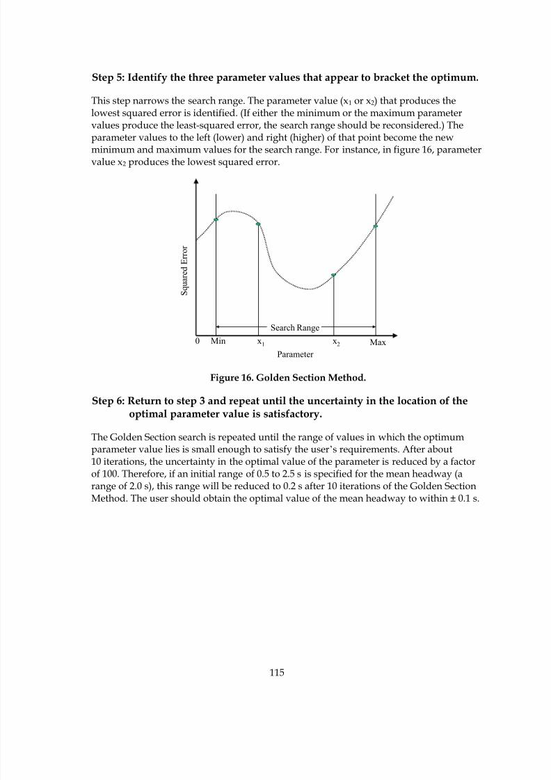
8/8/2019 Vol3 Guidelines
http://slidepdf.com/reader/full/vol3-guidelines 125/146
115
Step 5: Identify the three parameter values that appear to bracket the optimum.
This step narrows the search range. The parameter value (x1 or x2) that produces thelowest squared error is identified. (If either the minimum or the maximum parametervalues produce the least-squared error, the search range should be reconsidered.) The
parameter values to the left (lower) and right (higher) of that point become the newminimum and maximum values for the search range. For instance, in figure 16, parametervalue x2 produces the lowest squared error.
0 Min Maxx1 x2
S q u a r e
d E r r o r
Search Range
Parameter
Figure 16. Golden Section Method.
Step 6: Return to step 3 and repeat until the uncertainty in the location of the
optimal parameter value is satisfactory.
The Golden Section search is repeated until the range of values in which the optimumparameter value lies is small enough to satisfy the user’s requirements. After about10 iterations, the uncertainty in the optimal value of the parameter is reduced by a factorof 100. Therefore, if an initial range of 0.5 to 2.5 s is specified for the mean headway (arange of 2.0 s), this range will be reduced to 0.2 s after 10 iterations of the Golden SectionMethod. The user should obtain the optimal value of the mean headway to within ± 0.1 s.
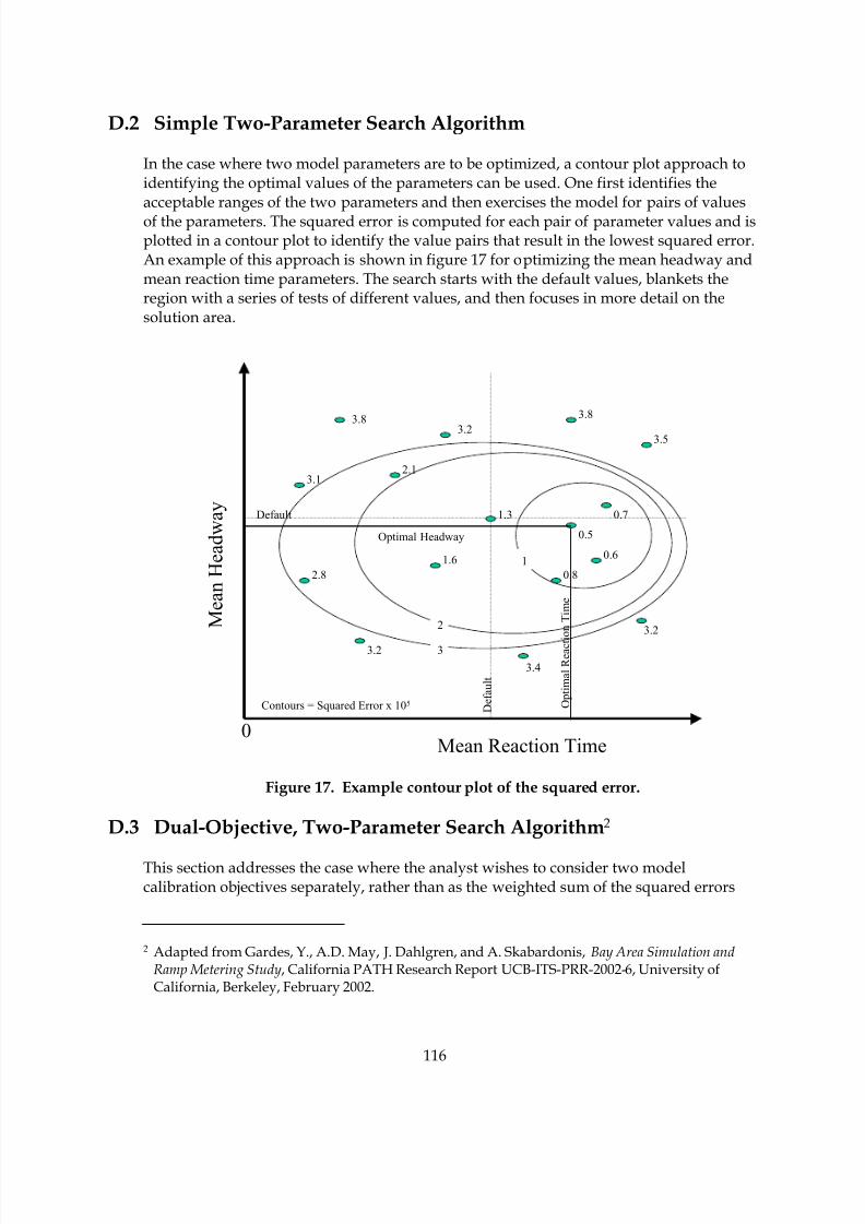
8/8/2019 Vol3 Guidelines
http://slidepdf.com/reader/full/vol3-guidelines 126/146
116
D.2 Simple Two-Parameter Search Algorithm
In the case where two model parameters are to be optimized, a contour plot approach toidentifying the optimal values of the parameters can be used. One first identifies theacceptable ranges of the two parameters and then exercises the model for pairs of valuesof the parameters. The squared error is computed for each pair of parameter values and isplotted in a contour plot to identify the value pairs that result in the lowest squared error.An example of this approach is shown in figure 17 for optimizing the mean headway andmean reaction time parameters. The search starts with the default values, blankets theregion with a series of tests of different values, and then focuses in more detail on thesolution area.
0
M e a n H e a d w a y
Mean Reaction Time
3.8
3.1
3.2
2.1
2.8
1.6
3.2
3.8
3.5
0.6
0.8
0.5
0.71.3
3.2
3.4
Default
D e f a u l t
3
2
1
Contours = Squared Error x 105
Optimal Headway
O p t i m a l R e a c t
i o n T i m e
Figure 17. Example contour plot of the squared error.
D.3 Dual-Objective, Two-Parameter Search Algorithm2
This section addresses the case where the analyst wishes to consider two modelcalibration objectives separately, rather than as the weighted sum of the squared errors
2 Adapted from Gardes, Y., A.D. May, J. Dahlgren, and A. Skabardonis, Bay Area Simulation andRamp Metering Study, California PATH Research Report UCB-ITS-PRR-2002-6, University ofCalifornia, Berkeley, February 2002.
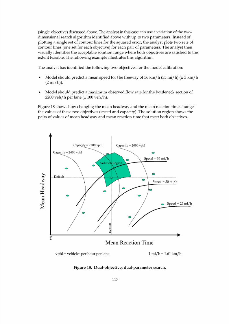
8/8/2019 Vol3 Guidelines
http://slidepdf.com/reader/full/vol3-guidelines 127/146
117
(single objective) discussed above. The analyst in this case can use a variation of the two-dimensional search algorithm identified above with up to two parameters. Instead ofplotting a single set of contour lines for the squared error, the analyst plots two sets ofcontour lines (one set for each objective) for each pair of parameters. The analyst thenvisually identifies the acceptable solution range where both objectives are satisfied to the
extent feasible. The following example illustrates this algorithm.
The analyst has identified the following two objectives for the model calibration:
• Model should predict a mean speed for the freeway of 56 km/h (35 mi/h) (± 3 km/h(2 mi/h)).
• Model should predict a maximum observed flow rate for the bottleneck section of2200 veh/h per lane (± 100 veh/h).
Figure 18 shows how changing the mean headway and the mean reaction time changes
the values of these two objectives (speed and capacity). The solution region shows thepairs of values of mean headway and mean reaction time that meet both objectives.
0
M e a n H e a d w a y
Mean Reaction Time
Default
D e f a u l t
Solution Region
Speed = 25 mph
Speed = 30 mph
Speed = 35 mph
Capacity = 2400 vphl
Capacity = 2200 vphl Capacity = 2000 vphl
vphl = vehicles per hour per lane 1 mi/h = 1.61 km/h
Figure 18. Dual-objective, dual-parameter search.
Speed = 35 mi/h
Speed = 30 mi/h
Speed = 25 mi/h

8/8/2019 Vol3 Guidelines
http://slidepdf.com/reader/full/vol3-guidelines 128/146
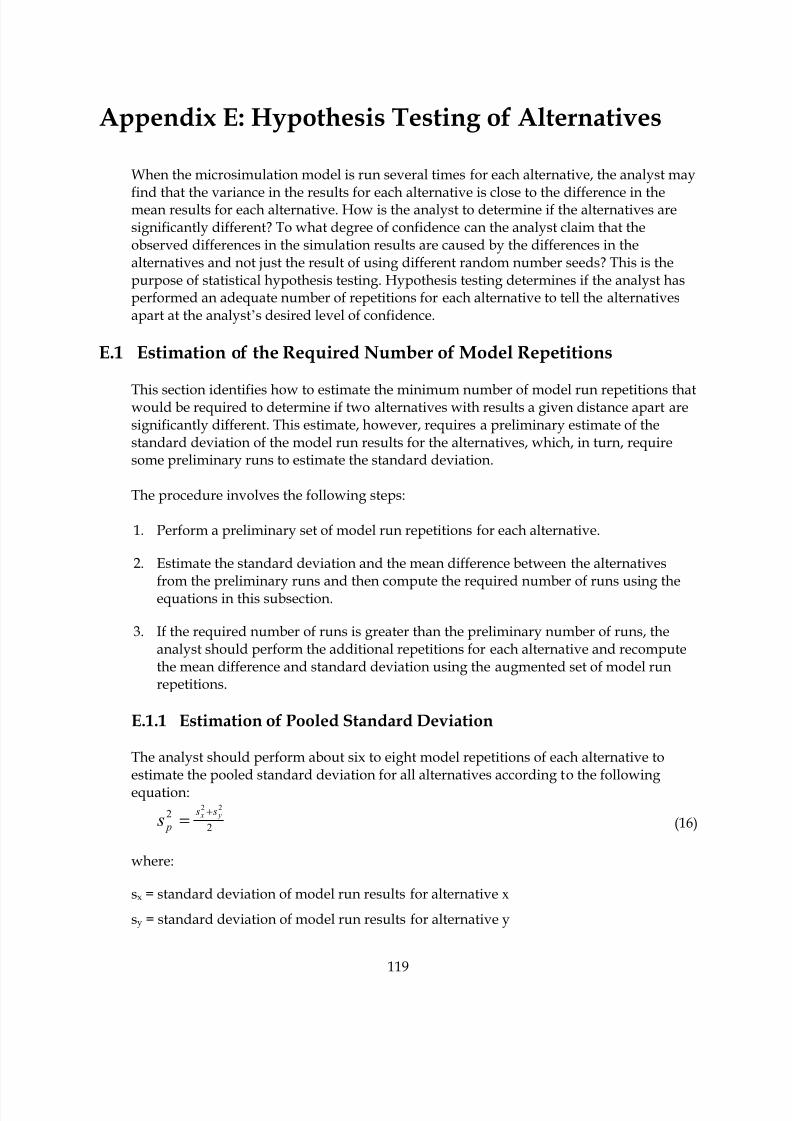
8/8/2019 Vol3 Guidelines
http://slidepdf.com/reader/full/vol3-guidelines 129/146
119
Appendix E: Hypothesis Testing of Alternatives
When the microsimulation model is run several times for each alternative, the analyst may
find that the variance in the results for each alternative is close to the difference in themean results for each alternative. How is the analyst to determine if the alternatives aresignificantly different? To what degree of confidence can the analyst claim that theobserved differences in the simulation results are caused by the differences in thealternatives and not just the result of using different random number seeds? This is thepurpose of statistical hypothesis testing. Hypothesis testing determines if the analyst hasperformed an adequate number of repetitions for each alternative to tell the alternativesapart at the analyst’s desired level of confidence.
E.1 Estimation of the Required Number of Model Repetitions
This section identifies how to estimate the minimum number of model run repetitions thatwould be required to determine if two alternatives with results a given distance apart aresignificantly different. This estimate, however, requires a preliminary estimate of thestandard deviation of the model run results for the alternatives, which, in turn, requiresome preliminary runs to estimate the standard deviation.
The procedure involves the following steps:
1. Perform a preliminary set of model run repetitions for each alternative.
2. Estimate the standard deviation and the mean difference between the alternatives
from the preliminary runs and then compute the required number of runs using theequations in this subsection.
3. If the required number of runs is greater than the preliminary number of runs, theanalyst should perform the additional repetitions for each alternative and recomputethe mean difference and standard deviation using the augmented set of model runrepetitions.
E.1.1 Estimation of Pooled Standard Deviation
The analyst should perform about six to eight model repetitions of each alternative toestimate the pooled standard deviation for all alternatives according to the followingequation:
2
222 y x s s
p s+
= (16)
where:
sx = standard deviation of model run results for alternative x
sy = standard deviation of model run results for alternative y

8/8/2019 Vol3 Guidelines
http://slidepdf.com/reader/full/vol3-guidelines 130/146
120
The preliminary model repetitions used to estimate the pooled estimate of the standarddeviation of the model run results can also be used to estimate the likely difference of themeans for each alternative.
E.1.2 Selection of Desired Confidence Level
A 95-percent confidence level is often selected for hypothesis testing. This means thatthere is a 5-percent chance (often called “alpha” in the textbooks) that the analyst willmistakenly reject the null hypothesis when it is really true (type I error). If a higherconfidence level is desirable, it comes at the cost of increasing the likelihood of making atype II error (accepting the null hypothesis when it is really false) (table 9).
Table 9. Null hypothesis.
True False
Accept Hypothesis OK Type II Error
Reject Hypothesis Type I Error OK
The study objective may determine the desired confidence level. For example, if theobjective is to design an alternative with a 95-percent probability that it will providesignificant improvements over the current facility, then this is the appropriate confidencelevel for the determination of the number of model repetitions required.
E.1.3 Selection of Minimal Difference in the Means
The likely minimal difference in the means between the alternatives should be identifiedby the analyst. This is the target sensitivity of the simulation tests of the alternatives.Alternatives with mean results farther apart than this minimal difference will obviouslybe different. Alternatives with mean results closer together than this minimal differencewill be considered to be indistinguishable.
The study objectives have some bearing on the selection of the minimal difference to be
detected by the simulation tests. If the study objective is to design a highwayimprovement that reduces mean delay by at least 10 percent, then the tests should bedesigned to detect if the alternatives are at least 10 percent apart.
The preliminary model repetitions used to estimate the pooled estimate of the standarddeviation of the model run results can also be used to estimate the likely difference of themeans for each alternative. The smallest observed difference in these preliminary runswould be the selected minimal difference of the means to be used in determining therequired number of repetitions.

8/8/2019 Vol3 Guidelines
http://slidepdf.com/reader/full/vol3-guidelines 131/146
121
E.1.4 Computation of Minimum Repetitions
Assuming that the analyst wishes to reject the null hypothesis that the means of the twomost similar alternatives are equal with only an alpha percent chance of error against thecounter hypothesis that the mean of alternative x is different than y, then the number of
repetitions required can be computed according to the following equation:3
n pn st y x 222);2/1( •>− −−α (17)
where:
=− y x absolute value of the estimated difference between the mean values for the two
most similar alternatives x and y
sp = pooled estimate of the standard deviation of the model run results for each alternative
n = number of model repetitions required for each alternative
t = t statistic for a confidence level of 1-alpha and 2n-2 degrees of freedom4
Note that when solving this equation for N, it is necessary to iterate until the estimatednumber of repetitions matches the number of repetitions assumed when looking up the tstatistic. Table 10 provides solutions for this equation for various target mean differenceranges and levels of confidence.
3 If the analyst intends to perform hypothesis tests on only a few pairs of alternatives, then the
equation provided should be sufficiently accurate. However, if the analyst plans to performhypothesis testing of all possible pairs of alternatives, then this equation will underestimate therequired number of repetitions needed to achieve the desired confidence level. The analystshould consult Lane, D.M., Hyperstat OnLine, An Introductory Statistics Book and Online Tutorial for Help in Statistics, Chapter 12: Introduction to Between-Subjects ANOVA (“All pairwisecomparisons among means…”), Rice University (www.davidmlane.com/hyperstat).
4 Note that this is a two-sided t-test for the null hypothesis that the means are equal versus thehypothesis that they are different.
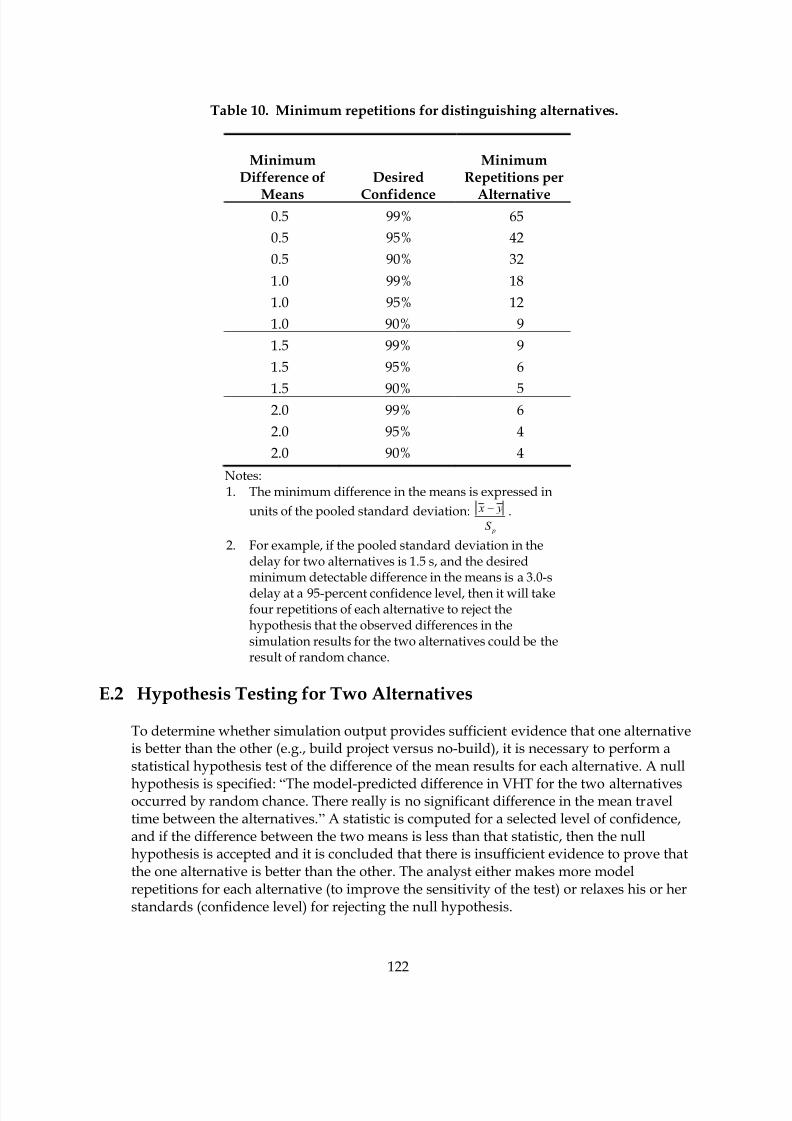
8/8/2019 Vol3 Guidelines
http://slidepdf.com/reader/full/vol3-guidelines 132/146
122
Table 10. Minimum repetitions for distinguishing alternatives.
MinimumDifference of
Means
Desired
Confidence
MinimumRepetitions per
Alternative0.5 99% 65
0.5 95% 42
0.5 90% 32
1.0 99% 18
1.0 95% 12
1.0 90% 9
1.5 99% 9
1.5 95% 6
1.5 90% 52.0 99% 6
2.0 95% 4
2.0 90% 4
Notes:1. The minimum difference in the means is expressed in
units of the pooled standard deviation:
pS
y x − .
2. For example, if the pooled standard deviation in thedelay for two alternatives is 1.5 s, and the desiredminimum detectable difference in the means is a 3.0-s
delay at a 95-percent confidence level, then it will takefour repetitions of each alternative to reject thehypothesis that the observed differences in thesimulation results for the two alternatives could be theresult of random chance.
E.2 Hypothesis Testing for Two Alternatives
To determine whether simulation output provides sufficient evidence that one alternativeis better than the other (e.g., build project versus no-build), it is necessary to perform astatistical hypothesis test of the difference of the mean results for each alternative. A null
hypothesis is specified: “The model-predicted difference in VHT for the two alternativesoccurred by random chance. There really is no significant difference in the mean traveltime between the alternatives.” A statistic is computed for a selected level of confidence,and if the difference between the two means is less than that statistic, then the nullhypothesis is accepted and it is concluded that there is insufficient evidence to prove thatthe one alternative is better than the other. The analyst either makes more modelrepetitions for each alternative (to improve the sensitivity of the test) or relaxes his or herstandards (confidence level) for rejecting the null hypothesis.

8/8/2019 Vol3 Guidelines
http://slidepdf.com/reader/full/vol3-guidelines 133/146
123
The specification of the problem is:
Null Hypothesis:
0:0 =− y x H µ µ (18)
against
0:1 ≠− y x H µ µ (19)
where:
µx = mean VHT (or some other measure) for alternative x
µy = mean for alternative y
This is a two-sided t-test with the following optimal rejection region for a given alpha(acceptable type I error):
mn pmn st y x 11)2();2/1( +•>− −+−α (20)
where:
=− y x absolute value of the difference in the mean results for alternative x and
alternative y
sp = pooled standard deviation
t = Student’s t-distribution for a level of confidence of 1-alpha and n+m-2 degrees offreedom
n = sample size for alternative x
m = sample size for alternative y
( ) ( )
( )2
11222
−+
−+−=
nm
sm sn
p
y x s (21)
where:
sp = pooled standard deviation
sx = standard deviation of the results for alternative x
sy = standard deviation of the results for alternative y
n = sample size for alternative x
m = sample size for alternative y

8/8/2019 Vol3 Guidelines
http://slidepdf.com/reader/full/vol3-guidelines 134/146
124
The probability of mistakenly accepting the null hypothesis is alpha (usually set to 5percent to get a 95-percent confidence level test). This is a type I error.
There is also a chance of mistakenly rejecting the null hypothesis. This is called a type IIerror and it varies with the difference between the sample means, their standard
deviation, and the sample size.5
E.3 Hypothesis Testing for Multiple Alternatives
When performing hypothesis testing on more than one pair of alternatives, it is mostefficient to first determine if any of the alternatives are significantly different from theothers. An analysis of variance (ANOVA) test is performed to determine if the meanresults for any of the alternatives are significantly different from the others:
• If the answer is yes, the analyst goes on to test specific pairs of alternatives.
• If the answer is no, the analysis is complete, or the analyst runs more modelrepetitions for each alternative to improve the ability of the ANOVA test todiscriminate among the alternatives.
E.3.1 Analysis of Variance (ANOVA) Test
The ANOVA test has three basic requirements:
• Independence of samples (random samples).
• Normal sampling distribution of means.
• Equal variances of groups.
Levine’s test of heteroscedasticity can be used for testing whether or not the variances ofthe model run results for each alternative are similar. Less powerful nonparametric tests,such as the Kruskal-Wallis test (K-W statistic) can be performed if the requirements of theANOVA test cannot be met.
However, the ANOVA test is tolerant of modest violations of these requirements and maystill be a useful test under these conditions. The ANOVA test will tend to be conservativeif its requirements are not completely met (less likely to have a type I error with a lowerpower of the test to correctly reject the null hypothesis).
5 Analysts should consult standard statistical textbooks for tables on the type II errors associatedwith different confidence intervals and sample sizes.

8/8/2019 Vol3 Guidelines
http://slidepdf.com/reader/full/vol3-guidelines 135/146
125
To perform the ANOVA test, first compute the test statistic:
SW
MSB F = (22)
where:
F = test statistic
MSB = mean square error between the alternatives (formula provided below)
MSW = mean square error among the model results for the same alternative (withinalternatives)
The formulas below show how to compute MSB and MSW:
1
)(1
2
−
−•
=
∑=
g
x xn
MSB
g
i
ii
(23)
where:
MSB = mean square error between the alternatives (i = 1 to g)
ni = number of model runs with different random number seeds for alternative i
=i x mean value for alternative i
= x mean value averaged across all alternatives and runs
g = number of alternatives
and
g N
sn
MSW
g
i
ii
−
•−
=∑=1
2)1(
(24)
where:
MSB = mean square error between the alternatives (i = 1 to g)
ni = number of model runs with different random number seeds for alternative i
=2
i s variance of the model run results for alternative i
N = total number of model runs summed over all alternatives
g = number of alternatives
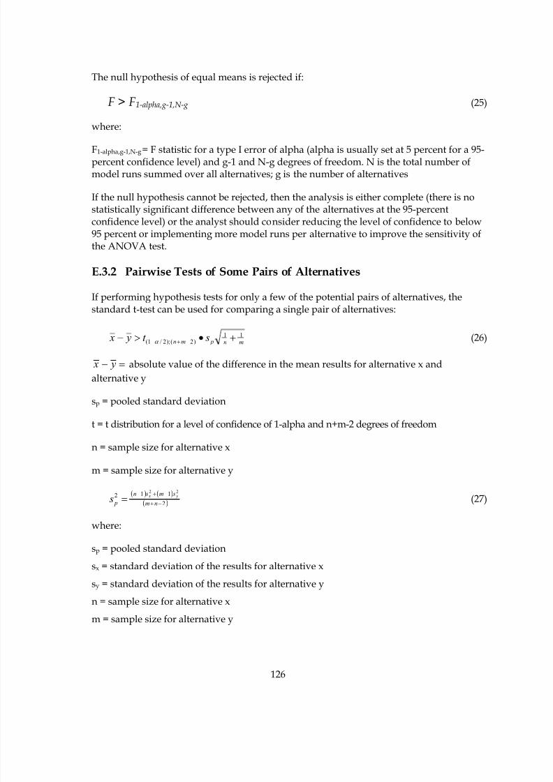
8/8/2019 Vol3 Guidelines
http://slidepdf.com/reader/full/vol3-guidelines 136/146
126
The null hypothesis of equal means is rejected if:
F > F 1-alpha,g-1,N-g (25)
where:
F1-alpha,g-1,N-g = F statistic for a type I error of alpha (alpha is usually set at 5 percent for a 95-percent confidence level) and g-1 and N-g degrees of freedom. N is the total number ofmodel runs summed over all alternatives; g is the number of alternatives
If the null hypothesis cannot be rejected, then the analysis is either complete (there is nostatistically significant difference between any of the alternatives at the 95-percentconfidence level) or the analyst should consider reducing the level of confidence to below95 percent or implementing more model runs per alternative to improve the sensitivity ofthe ANOVA test.
E.3.2 Pairwise Tests of Some Pairs of Alternatives
If performing hypothesis tests for only a few of the potential pairs of alternatives, thestandard t-test can be used for comparing a single pair of alternatives:
mn pmn st y x 11)2();2/1( +•>− −+−α (26)
=− y x absolute value of the difference in the mean results for alternative x and
alternative y
sp = pooled standard deviation
t = t distribution for a level of confidence of 1-alpha and n+m-2 degrees of freedom
n = sample size for alternative x
m = sample size for alternative y
( ) ( )
( )2
11222
−+
−+−=
nm
sm sn
p
y x s (27)
where:
sp = pooled standard deviation
sx = standard deviation of the results for alternative x
sy = standard deviation of the results for alternative y
n = sample size for alternative x
m = sample size for alternative y
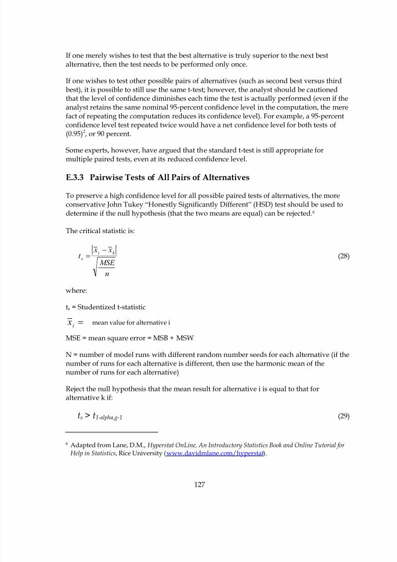
8/8/2019 Vol3 Guidelines
http://slidepdf.com/reader/full/vol3-guidelines 137/146
127
If one merely wishes to test that the best alternative is truly superior to the next bestalternative, then the test needs to be performed only once.
If one wishes to test other possible pairs of alternatives (such as second best versus thirdbest), it is possible to still use the same t-test; however, the analyst should be cautioned
that the level of confidence diminishes each time the test is actually performed (even if theanalyst retains the same nominal 95-percent confidence level in the computation, the merefact of repeating the computation reduces its confidence level). For example, a 95-percentconfidence level test repeated twice would have a net confidence level for both tests of(0.95)2, or 90 percent.
Some experts, however, have argued that the standard t-test is still appropriate formultiple paired tests, even at its reduced confidence level.
E.3.3 Pairwise Tests of All Pairs of Alternatives
To preserve a high confidence level for all possible paired tests of alternatives, the moreconservative John Tukey “Honestly Significantly Different” (HSD) test should be used todetermine if the null hypothesis (that the two means are equal) can be rejected.6
The critical statistic is:
n
MSE
x xt
k i
s
−= (28)
where:
ts = Studentized t-statistic
=i x
mean value for alternative i
MSE = mean square error = MSB + MSW
N = number of model runs with different random number seeds for each alternative (if thenumber of runs for each alternative is different, then use the harmonic mean of thenumber of runs for each alternative)
Reject the null hypothesis that the mean result for alternative i is equal to that foralternative k if:
ts > t1-alpha,g-1 (29)
6 Adapted from Lane, D.M., Hyperstat OnLine, An Introductory Statistics Book and Online Tutorial for Help in Statistics, Rice University (www.davidmlane.com/hyperstat).

8/8/2019 Vol3 Guidelines
http://slidepdf.com/reader/full/vol3-guidelines 138/146
128
where:
t1-alpha,g-1 = t statistic for a desired type I error of alpha (alpha is usually set at 5 percent toobtain a 95-percent confidence level) and g-1 degrees of freedom, with g equal to the totalnumber of alternatives tested, not just the two being compared in each test
Some experts consider the HSD test to be too conservative, failing to reject the nullhypothesis of equal means when it should be rejected. The price of retaining a highconfidence level (the same as retaining a low probability of a type I error) is a significantlyincreased probability of making a type II error (accepting the null hypothesis when it isreally false).
E.4 What To Do If the Null Hypothesis Cannot Be Rejected
If the null hypothesis of no significant difference in the mean results for the alternativescannot be rejected, then the analyst has the following options:
• Increase the number of model run repetitions per alternative until the simulationperformance of one alternative can be distinguished from the other.
• Reduce the confidence level from 95 percent to a lower level where the twoalternatives are significantly different and report the lower confidence level in theresults.
• Accept the result that the two alternatives are not significantly different.

8/8/2019 Vol3 Guidelines
http://slidepdf.com/reader/full/vol3-guidelines 139/146
129
Appendix F: Demand Constraints
Microsimulation results are highly sensitive to the amount by which the demand exceeds
the capacity of the facility, so it is vital that realistic demand forecasts be used in theanalysis. The following steps outline a procedure for manually reducing the forecasteddemands in the study area to better match the capacity of the facilities feeding the studyarea.
Step 1: Identify Gateway Bottlenecks
The analyst should first identify the critical bottlenecks on the facilities feeding the trafficto the boundaries of the microsimulation study area. Bottlenecks are sections of thefacilities feeding the model study area that either have capacities less than other sectionsof the freeway or demands greater than the other sections. These are the locations that will
probably be the first ones to experience congested conditions as traffic grows.
These bottlenecks may be located on the boundary of the microsimulation study area, inwhich case they are identical to the gateway zones on the boundary of themicrosimulation model study area. Bottlenecks within the microsimulation model studyarea can be disregarded since they will be taken into account by the microsimulationmodel.
Inbound bottlenecks are congested sections feeding traffic to the microsimulation modelarea. Outbound bottlenecks are congested sections affecting traffic leaving themicrosimulation model area. If an outbound bottleneck will probably create future queuesthat will back up into the microsimulation model study area, then the model study areashould be extended outward to include the outbound bottleneck. If the future outboundqueues will not back up into the model study area, then these bottlenecks can be safelydisregarded.

8/8/2019 Vol3 Guidelines
http://slidepdf.com/reader/full/vol3-guidelines 140/146
130
Microsimulation
Model Study Area
Bottleneck
Gateway
Figure 19. Bottleneck, gateway, and study area.
Step 2: Estimate Excess Demand at Inbound Bottlenecks
If the forecasted hourly demand at a bottleneck (in the inbound direction toward themodel) exceeds its capacity, the proportion of the demand that is in excess of the availablehourly capacity should be computed:
C
C D X
−= (30)
where:
X = proportion of excess demand
D = forecasted demand (veh/h)
C = estimated capacity (veh/h)
Step 3: Reduce Forecasted Demand Inbound at Gateways
The forecasted hourly demands for the off-ramps between the bottleneck and the gateway
entering the microsimulation study area should be reduced in proportion to the amountby which the forecasted bottleneck demand exceeds its capacity:
)1(* X D D unconst const −= (31)
where:
Dconst = constrained demand (veh/h) for a downstream off-ramp or exit point
Dunconst = unconstrained demand forecast (veh/h)
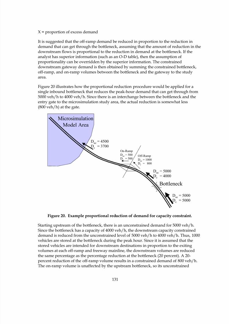
8/8/2019 Vol3 Guidelines
http://slidepdf.com/reader/full/vol3-guidelines 141/146
131
X = proportion of excess demand
It is suggested that the off-ramp demand be reduced in proportion to the reduction indemand that can get through the bottleneck, assuming that the amount of reduction in thedownstream flows is proportional to the reduction in demand at the bottleneck. If the
analyst has superior information (such as an O-D table), then the assumption ofproportionality can be overridden by the superior information. The constraineddownstream gateway demand is then obtained by summing the constrained bottleneck,off-ramp, and on-ramp volumes between the bottleneck and the gateway to the studyarea.
Figure 20 illustrates how the proportional reduction procedure would be applied for asingle inbound bottleneck that reduces the peak-hour demand that can get through from5000 veh/h to 4000 veh/h. Since there is an interchange between the bottleneck and theentry gate to the microsimulation study area, the actual reduction is somewhat less(800 veh/h) at the gate.
Microsimulation
Model Area
Bottleneck
Duc = 5000Dc = 4000
Duc = 5000
Dc = 5000
Off-Ramp
Duc = 1000
Dc = 800
On-Ramp
Duc = 500
Dc = 500
Duc = 4500
Dc = 3700
Figure 20. Example proportional reduction of demand for capacity constraint.
Starting upstream of the bottleneck, there is an unconstrained demand for 5000 veh/h.Since the bottleneck has a capacity of 4000 veh/h, the downstream capacity constraineddemand is reduced from the unconstrained level of 5000 veh/h to 4000 veh/h. Thus, 1000vehicles are stored at the bottleneck during the peak hour. Since it is assumed that thestored vehicles are intended for downstream destinations in proportion to the exitingvolumes at each off-ramp and freeway mainline, the downstream volumes are reducedthe same percentage as the percentage reduction at the bottleneck (20 percent). A 20-percent reduction of the off-ramp volume results in a constrained demand of 800 veh/h.The on-ramp volume is unaffected by the upstream bottleneck, so its unconstrained

8/8/2019 Vol3 Guidelines
http://slidepdf.com/reader/full/vol3-guidelines 142/146
132
demand is unchanged at 500 veh/h. The demand that enters the microsimulation studyarea is equal to the constrained demand of 4000 veh/h leaving the bottleneck, minus the800 veh/h leaving the freeway on the off-ramp, plus 500 veh/h entering the freeway atthe on-ramp, which results in a constrained demand of 3700 veh/h.
8/8/2019 Vol3 Guidelines
http://slidepdf.com/reader/full/vol3-guidelines 143/146
133
Appendix G: Bibliography
G.1 Traffic Microsimulation Fundamentals
Revised Monograph on Traffic Flow Theory, N.H. Gartner, C.J. Messer, and A. Ruthi(editors), FHWA, 1994 (www.tfhrc.gov/its/tft).
May, A.D., Traffic Flow Fundamentals, Prentice Hall, Englewood Cliffs, NJ, 1990.
Ahmed, K.I., Modeling Drivers’ Acceleration and Lane Changing Behavior , Ph.D. Dissertation,Massachusetts Institute of Technology, Cambridge, MA, February 1999.
Elefteriadou, L., G. List, J. Leonard, H. Lieu, M. Thomas, R. Giguere, R. Brewish, andG. Johnson, “Beyond the Highway Capacity Manual: A Framework for Selecting SimulationModels in Traffic Operational Analyses,” Transportation Research Record 1678, NationalAcademy Press, 1999, pp. 96-106.
G.2 Calibration and Validation of Microsimulation Models
Abdullai, B., J. Sheu, and W. Recker, Simulation of ITS on the Irvine FOT Area Using“Paramics 1.5” Scalable Microscopic Traffic Simulator, Phase I: Model Calibration and Validation, California PATH Program Research Report UCB-ITS-PRR-99-12, University of California,Berkeley, 1999.
Ben-Akiva, M., A. Davol, T. Toledo, H.N. Koutsopoulos, W. Burghout, I. Andréasson,T. Johansson, and C. Lundin, “Calibration and Evaluation of MITSIMLab in Stockholm,” Paper presented at the Annual Meeting, TRB, Washington, DC, 2002.
Fellendorf, M., and P. Vortisch, “Validation of the Microscopic Traffic Flow Model VISSIM inDifferent Real-World Situations,” Paper presented at the Annual Meeting, TRB, Washington,DC, 2001 (www.itc-world.com/library).
“Freeway System Operational Assessment,” Paramics Calibration and Validation Guidelines (Draft), Technical Report I-33, Wisconsin DOT, District 2, Milwaukee, WI, June 2002.
Gardes, Y., A.D. May, J. Dahlgren, and A. Skabardonis, Bay Area Simulation and Ramp Metering, California PATH Program Research Report.
Hellinga, B.R., Requirements for the Calibration of Traffic Simulation Models, Canadian Society ofCivil Engineering (CSCE), University of Waterloo, Ontario, Canada, 1998.
Jayakrishnan, R., J. Oh, and A.B. Sahraoui, Calibration and Path Dynamics Issues in MicroscopicSimulation for Advanced Traffic Management and Information Systems, UCI-ITS-WP-00-22,Institute of Transportation Studies, University of California, Irvine, December 2000.

8/8/2019 Vol3 Guidelines
http://slidepdf.com/reader/full/vol3-guidelines 144/146
134
Lee, D-H., X. Yang, and P. Chandrasekar, “Parameter Calibration for Paramics Using GeneticAlgorithm,” Paper No. 01-2339, Annual Meeting, TRB, Washington, DC, 2001.
Ma, T., and B. Abdulhai, “A Genetic Algorithm-Based Optimization Approach and GenericTool for the Calibration of Traffic Microscopic Simulation Parameters,” Paper presented at the
Annual Meeting, TRB, Washington, DC, 2002.
Owen, L.E., G. Brock, S. Mastbrook, R. Pavlik, L. Rao, C. Stallard, S. Sunkari, and Y. Zhang, ACompendium of Traffic Model Validation Documentation and Recommendations, FHWA ContractDTFH61-95-C-00125, FHWA, 1996.
Project Suite Calibration and Validation Procedures, Quadstone, Ltd., Edinburgh, UnitedKingdom, February 2000 (www.paramics-online.com/tech_support/ customer/cust_doc.htm (password required)).
Rakha, H., B. Hellinga, M. Van Aerde, and W. Perez, “Systematic Verification, Validation andCalibration of Traffic Simulation Models,” Paper presented at the Annual Meeting, TRB,Washington, DC, 1996.
Rao, L., L. Owen, and D. Goldsman, “Development and Application of a ValidationFramework for Traffic Simulation Models,” Proceedings of the 1998 Winter SimulationConference, D.J. Medeiros, E.F. Watson, J.S. Carson, and M.S. Manivannan (editors).
Skabardonis, A., Simulation of Freeway Weaving Areas, Preprint No. 02-3732, Annual Meeting,TRB, Washington, DC, 2002.
Traffic Appraisal in Urban Areas: Highways Agency, Manual for Roads and Bridges, Volume 12,Department for Transport, London, England, United Kingdom, May 1996
(www.archive.official-documents.co.uk/document/ha/dmrb/index.htm).
Wall, Z., R. Sanchez, and D.J. Dailey, A General Automata Calibrated With Roadway Data for Traffic Prediction, Paper No. 01-3034, Annual Meeting, TRB, Washington, DC, 2001.
G.3 Analysis of Results
Benekohal, R.F., Y.M. Elzohairy, and J.E. Saak, A Comparison of Delay From HCS, Synchro,Passer II, Passer IV, and CORSIM for an Urban Arterial, Preprint, Annual Meeting, TRB,Washington, DC, 2002.
Joshi, S.S., and A.K. Rathi, “Statistical Analysis and Validation of Multi-Population TrafficSimulation Experiments,” Transportation Research Record 1510, TRB, Washington, DC, 1995.
Prassas, E.S., A Comparison of Delay on Arterials by Simulation and HCM Computations, PreprintNo. 02-2652, Annual Meeting, TRB, Washington, DC, 2002.
Tian, Z.Z., T. Urbanik II, R. Engelbrecht, and K. Balke, Variations in Capacity and DelayEstimates From Microscopic Traffic Simulation Models, Preprint, Annual Meeting, TRB,Washington, DC, 2002.

8/8/2019 Vol3 Guidelines
http://slidepdf.com/reader/full/vol3-guidelines 145/146
135
Trueblood, M., “CORSIM…SimTraffic: What’s the Difference?,” PC-TRANS, Winter/Spring2001.
Gibra, I.N., Probability and Statistical Inference for Scientists and Engineers, Prentice-Hall,Englewood Cliffs, NJ, 1973.
Lane, D.M., Hyperstat OnLine, An Introductory Statistics Book and Online Tutorial for Help inStatistics, Rice University, Houston, TX (www.davidmlane.com/hyperstat).
Gerstman, B., and M. Innovera, StatPrimer, Version 5.1, California State University, San Jose(www.sjsu.edu/faculty/gerstman/StatPrimer).

8/8/2019 Vol3 Guidelines
http://slidepdf.com/reader/full/vol3-guidelines 146/146