volatility clustering in financial markets: empirical ... · volatility clustering in financial...

Volatility Clustering in Financial Markets:Empirical Facts and Agent–Based Models

Rama Cont�

Centre de Mathematiques appliquees, Ecole PolytechniqueF-91128 Palaiseau, France [email protected]

To appear in: A Kirman & G Teyssiere (eds.): Long memory in economics,Springer (2005).

Summary. Time series of financial asset returns often exhibit the volatility cluster-ing property: large changes in prices tend to cluster together, resulting in persistenceof the amplitudes of price changes. After recalling various methods for quantifyingand modeling this phenomenon, we discuss several economic mechanisms which havebeen proposed to explain the origin of this volatility clustering in terms of behaviorof market participants and the news arrival process. A common feature of thesemodels seems to be a switching between low and high activity regimes with heavy-tailed durations of regimes. Finally, we discuss a simple agent-based model whichlinks such variations in market activity to threshold behavior of market participantsand suggests a link between volatility clustering and investor inertia.

1 Introduction

The study of statistical properties of financial time series has revealed a wealthof interesting stylized facts which seem to be common to a wide variety ofmarkets, instruments and periods [12, 16, 25, 47]:

• Excess volatility: many empirical studies point out to the fact that itis difficult to justify the observed level of variability in asset returns byvariations in “fundamental” economic variables. In particular, the occur-rence of large (negative or positive) returns is not always explainable bythe arrival of new information on the market [15].

• Heavy tails: the (unconditional) distribution of returns displays a heavytail with positive excess kurtosis.

� The author thanks Alan Kirman and Gilles Teyssiere for their infinite patienceand participants in the CNRS Summer School on Complex Systems in the SocialSciences (ENS Lyon, 2004) for their stimulating feedback. The last section of thispaper is based on joint work with F. Ghoulmie and J.P. Nadal.

2 Rama Cont

• Absence of autocorrelations in returns: (linear) autocorrelations ofasset returns are often insignificant, except for very small intraday timescales (� 20 minutes) where microstructure effects come into play.

• Volatility clustering: as noted by Mandelbrot [40], “large changes tendto be followed by large changes, of either sign, and small changes tendto be followed by small changes.” A quantitative manifestation of thisfact is that, while returns themselves are uncorrelated, absolute returns|rt| or their squares display a positive, significant and slowly decayingautocorrelation function: corr(|rt|, |rt+τ |) > 0 for τ ranging from a fewminutes to a several weeks.

• Volume/volatility correlation: trading volume is positively correlatedwith market volatility. Moreover, trading volume and volatility show thesame type of “long memory” behavior [36].

Among these properties, the phenomenon of volatility clustering has intriguedmany researchers and oriented in a major way the development of stochasticmodels in finance –GARCH models and stochastic volatility models are in-tended primarily to model this phenomenon. Also, it has inspired much debateas to whether there is long-range dependence in volatility. We review some ofthese issues in Section 2. As noted by the participants of this econometric de-bate [54, 46], statistical analysis alone is not likely to provide a definite answerfor the presence or absence of long-range dependence phenomenon in stockreturns or volatility, unless economic mechanisms are proposed to understandthe origin of such phenomena.

Some insights into these economic mechanisms are given by agent-basedmodels of financial markets. Agent-based market models attempt to explainthe origin of the observed behavior of market prices in terms of simple, styl-ized, behavioral rules of market participants [11, 38, 39, 32]: in this approacha financial market is modeled as a system of heterogeneous, interacting agentsand several examples of such models have been shown to generate price be-havior similar to those observed in real markets. We review some of theseapproached in Section 3 and discuss how they lead to volatility clustering.

Most of these agent-based models are complex in structure and have beenstudied using Monte Carlo simulations. As noted also by LeBaron [31], due tothe complexity of such models it is often not clear which aspect of the model isresponsible for generating the stylized facts and whether all the ingredients ofthe model are indeed required for explaining empirical observations. In Section4 we present an agent-based model capable of generating time series of assetreturns with properties similar to the stylized facts above, but which is simpleenough in structure so the origins of volatility clustering can be traced backto agents behavior. This model points to a link between investor inertia andvolatility clustering and provide an economic explanation for the switchingmechanism proposed in the econometrics literature as an origin of volatilityclustering.

Volatility Clustering in Financial Markets 3

2 Volatility clustering in financial time series

Denote by St the price of a financial asset — a stock, an exchange rate or amarket index — and Xt = lnSt its logarithm. Given a time scale ∆, the logreturn at scale ∆ is defined as:

rt = Xt+∆ − Xt = ln(St+∆

St). (1)

∆ may vary between a minute (or even seconds) for tick data to several days.Observations are sampled at discrete times tn = n∆. Time lags will be denotedby the Greek letter τ ; typically, τ will be a multiple of ∆ in estimations. Forexample, if ∆ =1 day, corr[rt+τ , rt] denotes the correlation between the dailyreturn at period t and the daily return τ periods later.

2.1 Empirical behavior of autocorrelation functions

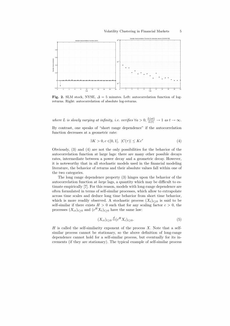
A typical display of daily log-returns is shown in figure 1: the volatility cluster-ing feature is seen graphically from the presence of sustained periods of highor low volatility. As noted above, the autocorrelation of returns is typicallyinsignificant at lags between a few minutes and a month. An example is shownin figure 2 (left). This “spectral whiteness” of returns can be attributed tothe activity of arbitrageurs who exploit linear correlations in returns via trendfollowing strategies [41]. By contrast, the autocorrelation function of absolutereturns remains positive over lags of several weeks and decays slowly to zero:figure 2 (right) shows this decay for SLM stock (NYSE). This observation isremarkably stable across asset classes and time periods and is regarded as atypical manifestation of volatility clustering [8, 13, 16, 25]. Similar behavioris observed for the autocorrelation of squared returns [8] and more generallyfor |rt|α [16, 17, 13] but it seems to be most significant for α = 1 i.e. absolutereturns [16].

GARCH models [8, 19] were among the first models to take into accountthe volatility clustering phenomenon. In a GARCH(1,1) model the (squared)volatility depends on last periods volatility:

rt = σtεt σ2t = a0 + aσ2

t−1 + bε2t 0 < a + b < 1 (2)

leading to positive autocorrelation in the volatility process σt, with a rate ofdecay governed by a + b: the closer a + b is to 1, the slower the decay of theautocorrelation of σt. The constraint a + b < 1 allows for the existence of astationary solution, while the upper limit a+ b = 1 corresponds to the case ofan integrated process. Estimations of GARCH(1,1) on stock and index returnsusually yield a + b very close to 1 [8]. For this reason the volatility clusteringphenomenon is sometimes called a “GARCH effect”; one should keep in mindhowever that volatility clustering is a “non-parametric” property and is notintrinsically linked to a GARCH specification.

4 Rama Cont

0.0 500.0 1000.0 1500.0-10.0

0.0

10.0

BMW stock daily returns

Fig. 1. Large changes cluster together: BMW daily log-returns. ∆ = 1 day.

While GARCH models give rise to exponential decay in autocorrelationsof absolute or squared returns, the empirical autocorrelations are similar to apower law [13, 25]:

C|r|(τ) = corr(|rt|, |rt+τ |) � c

τβ

with an exponent β ≤ 0.5 [13, 9], which suggests the presence of “long-range”dependence in amplitudes of returns, discussed below.

2.2 Long range dependence

Let us recall briefly the commonly used definitions of long range dependence,based on the autocorrelation function of a process:

Definition 1 (Long range dependence). A stationary process Yt (withfinite variance) is said to have long range dependence if its autocorrelationfunction C(τ) = corr(Yt, Yt+τ ) decays as a power of the lag τ :

C(τ) = corr(Yt, Yt+τ ) ∼τ→∞

L(τ)τ1−2d

0 < d <12

(3)


0 2 4 6 8 10 12 14 16 18 20−0.2

0

0.2

0.4

0.6

0.8

Lag

Sam

ple

Aut

ocor

rela

tion

Sample Autocorrelation Function (ACF)

0 2 4 6 8 10 12 14 16 18 20

10−2

10−1

100

Lag

Sample Autocorrelation Function for absolute returns (SLM:NYSE)

Fig. 2. SLM stock, NYSE, ∆ = 5 minutes. Left: autocorrelation function of log-returns. Right: autocorrelation of absolute log-returns.

where L is slowly varying at infinity, i.e. verifies ∀a > 0, L(at)L(t) → 1 as t → ∞.

By contrast, one speaks of “short range dependence” if the autocorrelationfunction decreases at a geometric rate:

∃K > 0, c ∈]0, 1[, |C(τ)| ≤ Kcτ (4)

Obviously, (3) and (4) are not the only possibilities for the behavior of theautocorrelation function at large lags: there are many other possible decaysrates, intermediate between a power decay and a geometric decay. However,it is noteworthy that in all stochastic models used in the financial modelingliterature, the behavior of returns and their absolute values fall within one ofthe two categories.

The long range dependence property (3) hinges upon the behavior of theautocorrelation function at large lags, a quantity which may be difficult to es-timate empirically [7]. For this reason, models with long-range dependence areoften formulated in terms of self-similar processes, which allow to extrapolateacross time scales and deduce long time behavior from short time behavior,which is more readily observed. A stochastic process (Xt)t≥0 is said to beself-similar if there exists H > 0 such that for any scaling factor c > 0, theprocesses (Xct)t≥0 and (cHXt)t≥0 have the same law:

(Xct)t≥0d=(cHXt)t≥0. (5)

H is called the self-similarity exponent of the process X. Note that a self-similar process cannot be stationary, so the above definition of long-rangedependence cannot hold for a self-similar process, but eventually for its in-crements (if they are stationary). The typical example of self-similar process

6 Rama Cont

whose increments exhibit long range dependence is fractional Brownian mo-tion [43].

But self-similarity does not imply long-range dependence in any way: α-stable Levy processes provide examples of self-similar processes with inde-pendent increments. Nor is self-similarity implied by long range dependence:Cheridito [10] gives several examples of Gaussian semimartingales with thesame long range dependence features as fractional Brownian noise but withno self-similarity (thus very different “short range” properties and sample pathbehavior). The example of fractional Brownian motion is thus misleading inthis regard, since it conveys the idea that these two properties are associated.When testing for long range dependence in a model based on fractional Brow-nian motion, we thus test the joint hypothesis of self-similarity and long-rangedependence and strict self-similarity is not observed to hold in asset returns[12, 13].

A fallacy often encountered in the literature is that long range depen-dence in returns is incompatible with absence of (continuous-time) arbitrage.Again, the origin of this idea can be traced back to models based on fractionalBrownian motion: since fractional Brownian motion is not a semimartingale, amodel in which the (log)-price are described by a fractional Brownian motionis not arbitrage-free (in the continuous-time sense) [51]. This result (and thefact that fractional Brownian motions fails to be a semimartingale) cruciallydepends on the local behavior of its sample paths, not on its long range depen-dence property. Cheridito [10] gives several examples of Gaussian processeswith the same long range dependence features as fractional Brownian motion,but which are semimartingales and lead to arbitrage-free models.

2.3 Dependence in stock returns

The volatility clustering feature indicates that asset returns are not indepen-dent across time; on the other hand the absence of linear autocorrelationshows that their dependence is nonlinear. Whether this dependence is “shortrange” or “long range” has been the object of many empirical studies.

The idea that stock returns could exhibit long range dependence was firstsuggested by Mandelbrot [41] and subsequently observed in many empiricalstudies using R/S analysis [42]. Such tests have been criticized by Lo [37] whopointed out that, after accounting for short range dependence, they mightyield a different result and proposed a modified test statistic. Lo’s statistichighly depends on the way “short range” dependence is accounted for andshows a bias towards rejecting long range dependence [53]. The final empiricalconclusions are therefore less clear [54].

However, the absence of long range dependence in returns may be compat-ible with its presence in absolute returns or “volatility”. As noted by Heyde[26], one should distinguish long range dependence in signs of increments,when sign(rt) verifies (3), from long range dependence in amplitudes, when|rt| verifies (3). Asset returns do not seem to possess long range dependence


in signs [26]. Many authors have thus suggested models, such as FIGARCH[4], in which returns have no autocorrelation but their amplitudes have longrange dependence [4, 18].

It has been argued [33, 5] that the decay of C|r|(τ) can also be reproducedby a superposition of several exponentials, indicating that the dependenceis characterized by multiple time scales. In fact, an operational definition oflong range dependence is that the time scale of dependence in a sample oflength T is found to be of the order of T : dependence extends over the wholesample. Interestingly, the largest time scale in [33] is found to be of the orderof...the sample size, a prediction which would be compatible with long-rangedependence!

Many of these studies test for long range dependence in returns, volatil-ity,.. by examining sample autocorrelations, Hurst exponents etc. but if timeseries of asset returns indeed possess the two features of heavy tails and longrange dependence, then many of the standard estimation procedures for thesequantities may fail to work [50]. For example, sample autocorrelation func-tions may fail to be consistent estimators of the true autocorrelation of returnsin the price generating process: Resnick and van der Berg [49] give examplesof such processes where sample autocorrelations converge to random values assample size grows! Also, in cases where the sample ACF is consistent, its esti-mation error can have a heavy-tailed asymptotic distribution, leading to largeerrors. The situation is even worse for autocorrelations of squared returns [45].Thus, one must be cautious in identifying behavior of sample autocorrelationwith the autocorrelations of the return process.

Slow decay of sample autocorrelation functions may possibly arise fromother mechanism than long-range dependence. For example, Mikosch & Star-ica [46] note that nonstationarity of the returns may also generate spuriouseffects which can be mistaken for long-range dependence in the volatility.However, we will not go to the extreme of suggesting, as in [46], that the slowdecay of sample autocorrelations of absolute returns is a pure artefact dueto non-stationarity. “Non-stationarity” does not suggest a modeling approachand it seems highly unlikely that unstructured non-stationarity would leadto such a robust, stylized behavior for the sample autocorrelations of abso-lute returns, stable across asset classes and time periods. The robustness ofthese empirical facts call for an explanation, which “non-stationarity” doesnot provide. Of course, these mechanisms are not mutually exclusive: a recentstudy by Granger and Hyng [24] illustrates the interplay of these two effectsby combining an underlying long memory process with occasional structuralbreaks.

Independently of the econometric debate on the “true nature” of the returngenerating process, one can take into account such empirical observationswithout pinpointing a specific stochastic model by testing for similar behaviorof sample autocorrelations in agent-based models (described below), and usingsample autocorrelations for indirect inference [22] of the parameters of suchmodels.

8 Rama Cont

3 Mechanisms for volatility clustering

While GARCH, FIGARCH and stochastic volatility models propose statisticalconstructions which mimick volatility clustering in financial time series, theydo not provide any economic explanation for it. We discuss here possiblemechanisms which have been proposed for the origin of volatility clustering.

3.1 Heterogeneous arrival rates of information

Heterogeneity in agent’s time scale has been considered as a possible origin forvarious stylized facts [25]. Long term investors naturally focus on long-termbehavior of prices, whereas traders aim to exploit short-term fluctuations.

Granger [23] suggested that long memory in economic time series can bedue to the aggregation of a cross section of time series with different persis-tence levels. This argument was proposed by Andersen & Bollerslev [1] as apossible explanation for volatility clustering in terms of aggregation of differ-ent information flows.

The effects of the diversity in time horizons on price dynamics have alsobeen studied by Lebaron [32] in an artificial stock market, showing that thepresence of heterogeneity in horizons may lead to an increase in return vari-ability, as well as volatility-volume relationships similar to those of actualmarkets.

3.2 Evolutionary models

Several studies have considered modeling financial markets by analogy withecological systems where various trading strategies co-exist and evolve viaa “natural selection” mechanism, according to their relative profitability[2, 3, 34, 32]. The idea of these models, the prototype of which is the SantaFe artificial stock market [3, 34], is that a financial market can be viewed asa population of agents, identified by their (set of) decision rules. A decisionrule is defined as a mapping from an agents information set (price history,trading volume, other economic indicators) to the set of actions (buy, sell, notrade). The evolution of agents decision rule is often modeled using a geneticalgorithm [27]. The specification and simulation of such evolutionary modelscan be quite involved and specialized simulation platforms have been devel-oped to allow the user to specify variants of agents strategies and evolutionrules. Other evolutionary models represent the evolution by a deterministicdynamical system which, through the complex price dynamics it generate, areable to mimick some “statistical” properties of the returns process, includingvolatility clustering [28].

Though the Santa Fe market model is capable of qualitatively replicatingsome of the stylized facts [34], precise comparisons with empirical observa-tions are still lacking. Indeed, given the large number of parameters, it is notpossible to calibrate the parameters in order to interpret the time periods


in the simulations as “days” or “minutes” etc. thereby leading to a lack ofreference for empirical comparisons.

More importantly, the competition between numerous strategies in suchcomplex simulation models does not allow to pinpoint a single mechanism asbeing responsible for volatility clustering or other stylized properties. Modelsin which a dominant mechanism is at work are more helpful in this respect;we will now discuss some instances of such models.

3.3 Behavioral switching

The economic literature contains examples where switching of economic agentsbetween two behavioral patterns leads to large aggregate fluctuations [29]: inthe context of financial markets, these behavioral patterns can be seen astrading rules and the resulting aggregate fluctuations as large movements inthe market price i.e. heavy tails in returns. Recently, models based on thisidea have also been shown to generate volatility clustering [30, 39].

Lux and Marchesi [39] study an agent-based model in which heavy tails ofasset returns and volatility clustering arise from behavioral switching of mar-ket participants between fundamentalist and chartist behavior. Fundamental-ists expect that the price follows the fundamental value in the long run. Noisetraders try to identify price trends, which results in a tendency to herding.Agents are allowed to switch between these two behaviors according to theperformance of the various strategies. Noise traders evaluate their performanceaccording to realized gains, whereas for the fundamentalists, performance ismeasured according to the difference between the price and the fundamentalvalue, which represents the anticipated gain of a “convergence trade”. Thisdecision-making process is driven by an exogenous fundamental value, whichfollows a Gaussian random walk. Price changes are brought about by a marketmaker reacting to imbalances between demand and supply. Most of the time,a stable and efficient market results. However, its usual tranquil performanceis interspersed by sudden transient phases of destabilization. An outbreak ofvolatility occurs if the fraction of agents using chartist techniques surpassesa certain threshold value, but such phases are quickly brought to an end bystabilizing tendencies. This behavioral switching is believed be the cause ofvolatility clustering, long memory and heavy tails in the Lux-Marchesi model[39].

Kirman and Teyssiere [30] have proposed a variant of [29] in which theproportion α(t) of fundamentalists in the market follows a Markov chain,of the type used in epidemiological models, describing herding of opinions.Simulation of this model exihibit autocorrelation patterns in absolute returnswith a behavior similar to that described in Section 2.

3.4 The role of investor inertia

As argued by Liu [35], the presence of a Markovian regime switching mecha-nism in volatility can lead to volatility clustering, is not sufficient to generate

10 Rama Cont

long-range dependence in absolute returns. More important than the switch-ing is the fact the time spent in each regime –the duration of regimes– shouldhave a heavy-tailed distribution [48, 52]. By contrast with Markov switch-ing, which leads to short range correlations, this mechanism has been called“renewal switching”.2

Bayraktar et al. [6] study a model where an order flow with random, heavy-tailed, durations between trades leads to long range dependence in returns.When the durations τn of the inactivity periods have a distribution of theform P(τn ≥ t) = t−αL(t), conditions are given under which, in the limit of alarge number of agents randomly submitting orders, the price process in thismodels converges to a a process with Hurst exponent H = (3 − α)/2 > 1/2.In this model the randomness (and the heavy tailed nature) of the durationsbetween trades are both exogenous ingredients, chosen in a way that generateslong range dependence in the returns. However, as noted above, empiricalobservations point to clustering and persistence in volatility rather than inreturns so such a result does not seem to be consistent with the stylized facts.

By contrast, as noted above, regime switching in volatility with heavy-tailed durations could lead to volatility clustering. Although in the agent-based models discussed above, it may not be easy to speak of well-defined“regimes” of activity, but Giardina and Bouchaud [21] argue that this is indeedthe mechanism which generates volatility clustering in the Lux-Marchesi [39]and other models discussed above. In these models, agents switch betweenstrategies based on their relative performance; Giardina and Bouchaud arguethat this (cumulative) relative performance index actually behaves in timelike a random walk, so the switching times can be interpreted as times whenthe random walk crosses zero: the interval between successive zero-crossingsis then known to be heavy-tailed, with a power-law decay of exponent 3/2.

4 Volatility clustering and threshold behavior

While switching between high and low volatility states is probably the mech-anism leading to volatility clustering in many of the agent-based models dis-cussed above, this explanation is not easy to trace back to the level of agentbehavior, partly because the models described above contain various other in-gredients whose contribution to the overall behavior is thus blurred. We nowdiscuss a simple model [14] reproducing several stylized empirical facts, wherethe origin of volatility clustering can be clearly traced back to investor inertia,caused by threshold response of investors to news arrivals.2 See the chapter by Giraitis, Leipus and Surgailis in this volume for a review on

renewal switching models.


4.1 An agent-based model for volatility clustering

Our model describes a market where a single asset, whose price is denoted bySt, is traded by N agents. Trading takes place at discrete periods t = 0, 1, 2, ...We will see that, provided the parameters of the model are chosen in a certainrange, we will be able to interpret these periods as “trading days”. At eachperiod, agents have the possibility to send an order to the market for buyingor selling a unit of asset: denoting by φi(t) the demand of the agent, we haveφi(t) = 1 for a buy order and φi(t) = −1. We allow the value φi(t) to bezero; the agent is then inactive at period t. The inflow of public informationis modeled by a sequence of IID Gaussian random variables (εt, t = 0, 1, 2, ..)with εt ∼ N(0,D2). εt represents the value of a common signal received by allagents at date t−1. The signal εt is a forecast of the future return rt and eachagent has to decide whether the information conveyed by εt is significant, inwhich case she will place a buy or sell order according to the sign of εt.

The trading rule of each agent i = 1, ..., N is represented by a (time–varying) decision threshold θi(t). The threshold θi(t) can be viewed as theagents (subjective) view on volatility. The trading rule we study may be seenas a stylized example of threshold behavior: without sufficient external stim-ulus (|εt| ≤ θi(t)), an agent remains inactive φi(t) = 0 and if the externalsignal is above a certain threshold, the agent will act: if εt > θi(t), φi(t) = 1,if εt < −θi(t), φi(t) = −1. The corresponding demand generated by the agentis therefore given by:

φi(t) = 1εt>θi(t) − 1εt<−θi(t). (6)

The excess demand is then given by Zt =∑N

i=1 φi(t). A non-zero value of Zproduces a change in the price given by

rt = lnSt

St−1= g(

Zt

N) (7)

where the price impact function g : R → R is an increasing function withg(0) = 0. We define the (normalized) market depth λ by : g′(0) = 1

λ . Examplesare a linear price impact g(z) = z/λ or g(z) = arctan(z/λ), both having beenused in various disequilibrium models.

Initially, we start from a population distribution F0 of thresholds: θi(0), i =1..N are positive IID variables drawn from F0. Updating of strategies is asyn-chronous: at each time step, any agent i has a probability 0 ≤ s ≤ 1 of updat-ing her threshold θi(t). Thus, in a large population, q represents the fractionof agents updating their views at any period; 1/q represents the typical timeperiod during which an agent will hold a given view θi(t). If periods are to beinterpreted as days, q is typically a small number s � 10−1 − 10−3. When anagent updates her threshold, she sets it to be equal to the recently observedabsolute return, which is an indicator of recent volatility |rt| = | ln St

St−1|. In-

troducing IID random variables ui(t), i = 1..N, t ≥ 0 uniformly distributed on[0, 1], which indicate whether agent i updates her threshold or not:

12 Rama Cont

θi(t) = 1ui(t)<s|rt| + 1ui(t)≥sθi(t − 1) (8)

This way of updating can be seen as a stylized version of various estimatorsof volatility based on moving averages of absolute or squared returns. It isalso corroborated by a recent empirical study by Zovko and Farmer [55], whoshow that traders use recent volatility as a signal when placing orders.

The asynchronous updating scheme proposed here avoids introducing anartificial ordering of agents as in sequential choice models. As noted above, theheterogeneity of time scales of intervention of agents is a feature believed to beimportant for generating persistence in volatility [1, 23, 31]. The random na-ture of updating in this model is a parsimonious way to introduce heterogene-ity in time scales without introducing extra parameters. Given this randomupdating scheme, even if we start from an initially homogeneous populationθi(0) = θ0, heterogeneity creeps into the population through the updatingprocess and evolves in a random manner, leading to a history-dependent dis-ordered system.

Let us recall the main ingredients of the model. At each time period:

1. agents receive a common signal ε(t) ∼ N(0,D2)2. each agent i compares the signal to her threshold θi(t)3. if |ε(t)| > θi(t) the agent considers the signal as significant and generates

an order φi(t) according to (6).4. The market price is impacted by the excess demand and moves according

to (7).5. Each agent updates, with probability q, her threshold according to (8).

Compared to most agent–based models considered in the literature, there isno exogenous “fundamental price” process and we do not distinguish between“fundamentalist” and “chartist” traders. Also, the same information is avail-able to all agents but they differ in the way they process the information. Wedo not introduce any “social interaction” among agents: no notion of locality,lattice or graph structure is introduced. The model has very few parameters:q describes the average updating frequency, D the standard deviation of thenoise representing the news arrival process, the market depth λ and the num-ber of agents N which is typically large. We will observe nevertheless thatthis simple model generates time series of returns with interesting dynamicsand properties similar to empirically observed properties of asset returns.

4.2 Simulation results

In order for a direct comparison with empirical stylized facts to be mean-ingful, we compute sample moments as in the case of empirical data, byaveraging over the (single) sample path. After simulating a sample path ofthe price St for T = 104 periods, we compute the time series of returnsrt = ln(St/St−1), t = 1..T , their histogram, a moving average estimator of the


standard deviation of returns (“volatility”), the sample autocorrelation func-tion of returns and the sample autocorrelation function of absolute returns.In order to decrease the sensitivity of results to initial conditions, we allowfor a transitory regime and discard the first 103 periods before averaging.

In order to interpret the trading periods as “days” and compare the resultswith properties of daily returns, we note that when g is linear |rt| ≤ 1

λ andchoose 5 ≤ λ ≤ 20 which allows a (maximal) range of daily returns between5% and 20%. Also, the amplitude D of the input noise can be chosen suchas to reproduce a realistic range of values for the (annualized) volatility: thisleads to choosing D in the range 10−3 − 10−2. Let us emphasize that we arediscussing the calibration of the order of magnitude of parameters, not fine–tuning them to a set of critical values. The results discussed in the sequelare generic within this range of parameters. Figures 3 and 4 illustrate typicalsample paths obtained with different parameter values: they all generate seriesof returns with realistic ranges and realistic values of annualized volatility.For each series, we represent the histogram of returns both in linear andlogarithmic scales, the ACF of returns Cr, the ACF of absolute returns C|r|.The return series obtained possess regularities which match the properties

0 5000 100000

200

400

600Market Activity

0 5000 100000

100

200

300

400Trading volume

0 5000 100000

0.5

1

1.5

2Price

0 5000 10000−0.05

0

0.05Log returns

0 5000 100000.1

0.2

0.3

0.4Annualized Moving average volatility

0 200 400 600

0

0.05

0.1

0.15

0.2Auto−correlation of returns

0 200 400 600−0.1

0

0.1

0.2

0.3Auto−correlation of absolute returns

−0.1 0 0.10

100

200

300

400Distribution of returns

−0.1 0 0.110

0

101

102

103

Distribution of returns

Fig. 3. Numerical simulation of the model with updating frequency q = 0.01 (aver-age updating period: 100 “days”) N = 1000 agents, D = 0.001 and λ = 10.

outlined in the introduction [14]:

14 Rama Cont

1. Excess volatility: the sample standard deviation of returns can be muchlarger than the standard deviation of the input noise representing newsarrivals σ(t) � D.

2. Mean-reverting volatility: the market price fluctuates endlessly and thevolatility, as measured by the moving average estimator σ(t), does neitherto zero nor to infinity and displays a mean-reverting behavior.

3. The simulated process generates a leptokurtic distribution of returns with(semi)heavy tails, with an excess kurtosis around κ � 7. As shown in thelogarithmic histogram plots in figures 3–4, the tails exhibit an approxi-mately exponential decay, as observed in various studies of daily returns[16].

4. The returns are uncorrelated: the sample autocorrelation function of thereturns exhibits an insignificant value (very similar to that of asset re-turns) at all lags, indicating the absence of linear serial dependence in thereturns.

5. Volatility clustering: the autocorrelation function of absolute returns re-mains significantly positive over many time lags, corresponding to persis-tence of the amplitude of returns a time scale � 1/q.

0 5000 100000

500

1000

1500Market Activity

0 5000 100000

500

1000

1500Trading volume

0 5000 100000

1

2

3

4Price

0 5000 10000−0.1

−0.05

0

0.05

0.1Log returns

−0.1 0 0.10

500

1000

1500Distribution of returns

−0.1 0 0.110

0

102

104

Distribution of returns

0 5000 100000.2

0.25

0.3Annualized Moving average volatility

0 200 400 600−0.2

−0.1

0

0.1

0.2

Auto−correlation of returns

0 20 40−0.2

0

0.2

0.4

0.6Auto−correlation of absolute returns

Fig. 4. Numerical simulation of the model with updating frequency q = 0.1 (averageupdating period: 10 “days”) N = 1500 agents, D = 0.001 and λ = 10.


4.3 Theoretical analysis

Contrarily to some of the models discussed above, this model is simple enoughto allow for a theoretical study of its qualitative studies [14]. Let us being byexamining two limiting cases:

1. Feedback without heterogeneity: In the case where q = 1, all agentssynchronously update their threshold at each period. Consequently, theagents have the same thresholds, given by the last periods absolute return:θi(t) = |rt−1| and will therefore generate the same order: Zt = Nφ1(t) ∈{0, N,−N}. So, the return rt depends on the past only through the abso-lute return |rt−1|:

rt = f(|rt−1, εt|) = g(N)1εt>|rt−1| + g(−N)1εt<−|rt−1|,

a dependence structure typical of ARCH models [19], leading to un-correlated returns and volatility clustering. In this case, the distribu-tion of rt conditional on |rt−1| is actually a trinomial distribution: rt ∈{0, g(N), g(−N)}, which is not realistic. Simulation studies show that asimilar behavior persists for 1− q � 1, leading to tri-modal distributions.This confirms our intuition that the updating probability q should bechosen small.

2. Heterogeneity without feedback: In the case where q = 0, no updat-ing takes places: the trading strategies, given by the thresholds θi, areunaffected by the price behavior and the feedback effect is not presentanymore. Heterogeneity is still present: the distribution of the thresholdsremains identical to what it was at t = 0. The return rt depends only onεt :

rt = g(1N

N∑

i=1

1εt>θi− 1εt<−θi

) = F (εt)

We conclude therefore that the returns are IID random variables, obtainedby transforming the Gaussian IID sequence (εt) by the nonlinear functionF given in (9), whose properties depend on the (initial) distribution ofthresholds (θi, i = 1..N). The log–price then follows a (non–Gaussian)random walk and the model does not exhibit volatility clustering.

The two limiting cases above show that, in order to obtain the interestingstatistical properties observed in the simulated examples shown above, it isnecessary to have 0 < q � 1: both feedback and heterogeneity are essentialingredients. In the general case we have the following properties:

• Markovian dynamics: the thresholds [θi(t), i = 1...N ] follow a Markovchain in {g(k), k = 0...N}. We have θi(t+1) = θi(t) with probability 1− qand

16 Rama Cont

θi(t + 1) = |rt| = |g(1N

N∑

i=1

[1εt>θi− 1εt<−θi

])| with probability q.(9)

In fact given that agents are indistinguishable and only the empiricaldistribution of threshold values affects the returns, defining Nk(t) =∑N

i=1 1[0,ak[(θi(t)) then (Nk(t), k = 0..N − 1)t=0,1,.. evolves as a Markovchain in {0, ..., N}N . N(t) = (Nk(t), k = 0..N − 1) is none other than the(cumulative) population distribution of the thresholds. The fact that N(t)itself follows a Markov chain means that the population distribution ofthresholds is a random measure on {0, ..., N}, which is characteristic ofdisordered systems [44], even if we start from a deterministic set of val-ues for the initial thresholds (even identical ones). Here the disorder isendogenous and is generated by the random updating mechanism.

• Excess volatility: In this model, the volatility of the news arrival processis quantified by D which is the standard deviation of the external noise εt,whereas the volatility of the returns can be measured a posteriori as the(conditional or unconditional) standard deviation of rt. As seen from thenonlinear relation between εt and rt,

rt = g(∑N

i=1 1εt>θi(t) − 1εt<−θi(t)

λN) (10)

even after conditioning on the current states of agents θi(t), i = 1..N ,Eq. (10) yields a nonlinear relation between the input noise εt and thereturns which can have the effect of amplifying the noise by an order ofmagnitude or more. In the simulation example shown in figure 3, D = 10−3

which corresponds to an annualized volatility of 1.6%, while the annualizedvolatility of returns is in the range of 20%, an order of magnitude larger:the order of magnitude of the volatility of returns may be quite differentfrom that of the input noise.

• Absence of autocorrelationFrom the dynamic equations of the model

Zt =1N

N∑

i=1

φi(t) =1N

N∑

i=1


] (11)

rt = g(Zt) = g(1N

N∑

i=1


]) (12)

one can deduce that, if g is an odd function (in particular if g is linear) thenasset returns (rt)t≥0 are uncorrelated: cov(rt, rt+1)=0. This is due to thefact that the trading/ nontrading decision is based only on the amplitudeof the signal, not its sign. The sign of the return is determined by the signof the common signal, which is independent across periods.

• Investor inertiaExcept in times of crisis or market crash, at a given point in time only


a small proportion of stockholders are actually trading in the market. Asa result, the (daily) order flow for a typical stock can be much smallerthan the market capitalization. This phenomenon, sometimes referred toas investor inertia, is a generic outcome in our model due to thresholdbehavior of agents. Starting from an initial holding of πi(0), the quantity ofasset held by agent i is given by πi(t) =

∑tτ=0 φi(τ). Figure 4.3 displays the

evolution of the portfolio πi(t) of a typical agent: short periods of activity(trading) are separated by long periods of inertia, where the portfolioremains constant. This “inertia” increases in periods of high volatility, an

0 1000 2000 3000 4000 5000 6000 7000 8000 9000 1000070

75

80

85

90

95

100

105

110

t

π i(t)

Fig. 5. Evolution of the portfolio of a typical agent, with long periods of inactivitypunctuated by bursts of activity.

effect similar to the behavior of risk-averse agent.• Mean reversion and clustering of volatility

Many market microstructure models –especially those with learning orevolution– converge over large time intervals to an equilibrium where pricesand other aggregate quantities cease to fluctuate randomly. By contrast,in the present model, prices fluctuate endlessly and the volatility exhibitsmean-reverting behavior. Suppose we are in a period of “low volatility”;the amplitude |rt| of returns is small. Agents who update their thresholdswill therefore update them to small values, become more sensitive to newsarrivals, thus generating higher excess demand and thus increasing theamplitude of returns. Conversely, in a period of high volatility, agents willupdate their threshold values to high values and become less reactive to

18 Rama Cont

the incoming signal: this increase in investor inertia will thus decrease theamplitude of returns. The mean reversion time in the volatility correspondshere to the time it takes for agents to adjust their thresholds to currentmarket conditions, which is of order τc = 1/q.When the amplitude of the noise is small it can be shown [14] that volatilitydecays exponentially in time and increases through upward “jumps”. Thisbehavior is actually similar to that of a class of stochastic volatility models,introduced by Barndorff-Nielsen and Shephard [5] and successfully used todescribe various econometric properties of returns.

5 Conclusion

Volatility clustering is recognized as a stylized property present in most fi-nancial time series. Agent-based models seek to explain volatility clusteringin terms of behavior of market participants, described in terms of simple rules.We have discussed several agent-based models capable of generating volatilityclustering. A common feature of these models seems to be the “switching” ofthe market between periods of high and low activity, with long durations ofperiods. Models differ in the mechanism which leadsz to this switching at thelevel of agents.

While the econometric debate on the short range or long range nature ofdependence in volatility still goes on (and may probably never be resolved),agent-based models can provide motivation for choosing between alternativeeconometric specifications which are otherwise equally plausible in statisticalterms, thus providing a useful complement to econometric analysis.

References

1. T. Andersen and T. Bollerslev, Heterogeneous information arrivals and returnsvolatility dynamics, Journal of finance, 52 (1997), pp. 975–1005.

2. J. Arifovic and R. Gencay, Statistical properties of genetic learning in a model ofexchange rate, Journal of Economic Dynamics and Control, 24 (2000), pp. 981–1005.

3. Arthur, W., Holland, J., LeBaron, B., Palmer, J. and Tayler, P. (1997). Assetpricing under heterogeneous expectations in an artificial stock market, in: TheEconomy as an Evolving Complex System. Perseus Books, Reading MA, pp.15–44.

4. Baillie, R.T. (1996). Long memory processes and fractional integration in econo-metrics. Journal of Econometrics, 73, 5–59.

5. O. E. Barndorff-Nielsen and N. Shephard (2001) Non-Gaussian Ornstein-Uhlenbeck based models and some of their uses in financial econometrics, Jour-nal of the Royal Statistical Society B, 63, pp. 167–241.

6. E. Bayraktar, U. Horst, and K. R. Sircar, A limit theorem for financial marketswith inert investors, working paper, Princeton University, 2003.


7. J. Beran, Statistics for long memory processes, Chapman and Hall, New York,1994.

8. T. Bollerslev, R. Chou, and K. Kroner, ARCH modeling in finance, Journal ofEconometrics, 52 (1992), pp. 5–59.

9. F. Breidt, N. Crato, and P. De Lima, The detection and estimation of longmemory in stochastic volatility, Journal of Econometrics, 83 (1998), pp. 325–348.

10. P. Cheridito, Gaussian moving averages, semimartingales and option pricing,Stochastic Process. Appl., 109 (2004), pp. 47–68.

11. C. Chiarella, M. Gallegatti, R. Leombruni, and A. Palestrini, Asset price dy-namics among heterogeneous interacting agents, Computational Economics, 22(2003), pp. 213–223.

12. R. Cont, Empirical properties of asset returns: Stylized facts and statisticalissues, Quantitative Finance, 1 (2001), pp. 1–14.

13. R. Cont, J.-P. Bouchaud, and M. Potters, Scaling in financial data: Stable lawsand beyond, in: B. Dubrulle, F. Graner, and D. Sornette (eds.) Scale Invarianceand Beyond, Springer, Berlin, 1997.

14. R. Cont, F. Ghoulmie, and J.-P. Nadal, Threshold behavior and volatility clus-tering in financial markets, Working paper, Ecole Polytechnique, 2004.

15. D. Cutler, J. Poterba, and L. Summers, What moves stock prices?, Journal ofPortfolio Management, (1989), pp. 4–12.

16. Z. Ding, C. Granger, and R. Engle, A long memory property of stock marketreturns and a new model, Journal of empirical finance, 1 (1983), pp. 83–106.

17. Z. Ding and C. W. J. Granger, Modeling volatility persistence of speculativereturns: a new approach, Journal of Econometrics, 73 (1996), pp. 185–215.

18. P. Doukhan, G. Oppenheim, and M. S. Taqqu, eds., Theory and applications oflong-range dependence, Birkhauser Boston Inc., Boston, MA, 2003.

19. R. Engle, ARCH models, Oxford University Press, Oxford, 1995.20. F. Ghoulmie, R. Cont and J.-P. Nadal, Heterogeneity and feedback in an agent-

based market model, Journal of Physics: Condensed Matter, 17, S1259-S1268(2005).

21. I. Giardina and J.-P. Bouchaud, Bubbles, crashes and intermittency in agentbased market models, Eur. Phys. Journal B ., 31 (2003), pp. 421–437.

22. C. Gourieroux, A. Monfort, and E. Renault, Indirect inference, Journal ofApplied Econometrics, 8 (1993), pp. S85–S118.

23. C. W. J. Granger, Long memory relationships and the aggregation of dynamicmodels, Journal of Econometrics, 14 (1980), pp. 227–238.

24. Granger, C.W.J. and Hyng, N. (2004) Occasional structural breaks and longmemory with an application to the S&P 500 absolute stock returns. Journal ofEmpirical Finance, 11, 399-421.

25. D. Guillaume, M. Dacorogna, R. Dave, U. Muller, R. Olsen, and O. Pictet,From the birds eye view to the microscope: A survey of new stylized facts of theintraday foreign exchange markets, Finance and Stochastics, 1 (1997), pp. 95–131.

26. C. C. Heyde, On modes of long-range dependence, Journal of Applied Proba-bility, 39 (2002), pp. 882–888.

27. J. Holland, Adaptation in Natural and Artificial Systems, Bradford Books, 1992.28. C. H. Hommes, A. Gaunersdorfer, and F. O. Wagener, Bifurcation routes to

volatility clustering under evolutionary learning, working paper, CenDEF, 2003.

20 Rama Cont

29. A. Kirman, Ants, rationality, and recruitment, Quarterly Journal of Economics,108 (1993), pp. 137–156.

30. A. Kirman and G. Teyssiere, Microeconomic models for long-memory in thevolatility of financial time series, Studies in nonlinear dynamics and economet-rics, 5 (2002), pp. 281–302.

31. B. LeBaron, Agent-based computational finance : suggested readings and earlyresearch, Journal of Economic Dynamics and Control, 24 (2000), pp. 679–702.

32. , Evolution and time horizons in an agent-based stock market, Macroeco-nomic Dynamics, 5 (2001), pp. 225–254.

33. , Stochastic volatility as a simple generator of apparent financial powerlaws and long memory, Quantitative Finance, 1 (2001), pp. 621–631.

34. B. LeBaron, B. Arthur, and R. Palmer, Time series properties of an artificialstock market, Journal of Economic Dynamics and Control, 23 (1999), pp. 1487–1516.

35. M. Liu, Modeling long memory in stock market volatility, Journal Economet-rics, 99 (2000), pp. 139–171.

36. Lobato, I. and Velasco, C. (2000) Long memory in stock market trading volume.Journal of Business and Economic Statistics, 18, 410-427.

37. A. Lo Long-term memory in stock market prices, Econometrica, 59 (1991),pp. 1279–1313.

38. T. Lux, The socio-economic dynamics of speculative markets : interactingagents, chaos, and the fat tail of return distributions, Journal of EconomicBehavior and Organization, 33 (1998), pp. 143–65.

39. T. Lux and M. Marchesi, Volatility clustering in financial markets : a micro sim-ulation of interacting agents, International Journal of Theoretical and AppliedFinance, 3 (2000), pp. 675–702.

40. B. B. Mandelbrot (1963) The variation of certain speculative prices, Journal ofBusiness, XXXVI (1963), pp. 392–417.

41. B. B. Mandelbrot (1971) When can price be arbitraged efficiently? A limit tothe validity of the random walk and martingale models, Rev. Econom. Statist.,53 (1971), pp. 225–236.

42. B. B. Mandelbrot and M. S. Taqqu, Robust R/S analysis of long-run serialcorrelation, in Proceedings of the 42nd session of the International StatisticalInstitute, Vol. 2 (Manila, 1979), vol. 48, 1979, pp. 69–99.

43. B. B. Mandelbrot and J. Van Ness, Fractional Brownian motion, fractionalnoises and applications, SIAM Review, 10 (1968), pp. 422–437.

44. M. Mezard, G. Parisi, and M. Virasoro, Spin glass theory and beyond, WorldScientific, 1984.

45. T. Mikosch and C. Starica, Limit theory for the sample autocorrelations andextremes of a GARCH (1, 1) process, Ann. Statist., 28 (2000), pp. 1427–1451.

46. , Long-range dependence effects and ARCH modeling, in Theory andapplications of long-range dependence, Birkhauser Boston, Boston, MA, 2003,pp. 439–459.

47. A. Pagan (1986). The econometrics of financial markets, Journal of empiricalfinance, 3, pp. 15–102.

48. M. Pourahmadi (1988) Stationarity of the solution of Xt = AtXt + 1 andanalysis of non-Gaussian dependent variables. Journal of Time Series Analysis,9, 225–239.

49. S. Resnick, G. Samorodnitsky, and F. Xue, How misleading can sample ACFsof stable MAs be? (Very!), Ann. Appl. Probab., 9 (1999), pp. 797–817.


50. S. I. Resnick, Why non-linearities can ruin the heavy-tailed modeler’s day, inA practical guide to heavy tails (Santa Barbara, CA, 1995), Birkhauser Boston,Boston, MA, 1998, pp. 219–239.

51. L. Rogers, Arbitrage with fractional Brownian motion, Mathematical Finance,7 (1997), pp. 95–105.

52. M. Taqqu and J. Levy, Using renewal processes to generate long range depen-dence and high variability, in Dependence in probability and statistics, E. Eber-lein and M. Taqqu, eds., Birkhauser, Boston, 1986, pp. 73–89.

53. V. Teverovsky, M. S. Taqqu, and W. Willinger, A critical look at Lo’s modifiedR/S statistic, J. Statist. Plann. Inference, 80 (1999), pp. 211–227.

54. W. Willinger, M. S. Taqqu, and V. Teverovsky, Long range dependence andstock returns, Finance and Stochastics, 3 (1999), pp. 1–13.

55. I. Zovko and J. D. Farmer, The power of patience: a behavioral regularity inlimit order placement, Quantitative Finance, 2 (2002), pp. 387–392.

volatility clustering in financial markets: empirical ... · volatility clustering in financial...

Documents