volatility modeling in financial marketssbhulai/papers/thesis-ladokhin.pdf · 2 summary this...
TRANSCRIPT
Volatility modeling in financial markets
Master Thesis
Sergiy Ladokhin
Supervisors:
Dr. Sandjai Bhulai, VU University Amsterdam
Brian Doelkahar, Fortis Bank Nederland
VU University Amsterdam
Faculty of Sciences, Business Mathematics and Informatics De Boelelaan 1081a, 1081 HV Amsterdam
Host organization: Fortis Bank Nederland, Brokerage Clearing and Custody
Rokin 55, 1012 KK Amsterdam
PUBLIC VERSION 26 July 2009

2
Summary
This project focuses on the problem of volatility modeling in financial markets. It begins with
a general description of volatility and its properties, and discusses its usage in financial risk
management. The research is divided into two parts: estimation of conditional volatility and modeling
of volatility skews. The first one is focused on comparing different models for conditional volatility
estimation. We examine the accuracy of several of the most popular methods: historical volatility
models (e.g., Exponential Weighted Moving Average), the implied volatility, and autoregressive
conditional heteroskedastic models (e.g., the GARCH family of models). The second part of the
project is dedicated to modeling the implied volatility skews and surfaces. We introduce a number of
representations of the volatility skews and discuss their importance for the risk management of the
options portfolio. The comparison analysis of several approaches to the volatility skews modeling
(including spline models and the SABR family of models) is made. Special attention is paid to
modeling the dynamics of the implied volatility surfaces in time.
This research is done for the Fortis Bank Nederland Brokerage, Clearing and Custody
(FBNBCC). All of the models and methods described in this research are designed to improve the
methodology currently used by FBNBCC. The models of this study were implemented, calibrated, and
tested using real market data; and their results were compared to the currently used methods by the
FBNBCC‘s risk management system. Another objective of this study is to examine potential
shortcomings of FBNCC’s risk management system and to develop recommendations for their
elimination.

3
Table of Contents
Summary ............................................................................................................................................ 2
1 Introduction.............................................................................................................................. 4
2 Comparison analysis of models for volatility forecasting ........................................................ 6
2.1 Role of volatility in the estimation of the market risk ......................................................... 6
2.2 Metrics for the market risk .................................................................................................. 8
2.3 Models for conditional volatility ........................................................................................ 11
2.4 Applications of Extreme Value Theory to the market risk ................................................. 18
2.5 Comparison of the volatility forecasting models ............................................................... 20
3 Modeling implied volatility surfaces ...................................................................................... 24
3.1 Risk of volatility “smile” and its impact .............................................................................. 24
3.2 Representation of the moneyness ..................................................................................... 25
3.3 Models of the implied volatility surface ............................................................................. 27
3.4 Modeling the dynamics of volatility surfaces ..................................................................... 35
3.5 Comparison of the volatility surface models ..................................................................... 40
4 Conclusions and practical recommendations ........................................................................ 45
5 Appendixes ............................................................................................................................. 46
5.1 t Location‐Scale distribution .............................................................................................. 46
5.2 The Black‐Scholes option pricing equation ........................................................................ 48
5.3 Cross‐ validation ................................................................................................................. 50
5.4 Results of the conditional volatility estimation ................................................................. 51
5.5 Results of implied volatility surface modeling ................................................................... 55
6 Bibliography ........................................................................................................................... 58

4
1 Introduction The main characteristic of any financial asset is its return which is typically considered to be a
random variable. The spread of outcomes of this variable, known as assets volatility, plays an
important role in numerous financial applications. Its primary usage is to estimate the value of
market risk. Volatility is also a key parameter for pricing financial derivatives. All modern option‐
pricing techniques rely on a volatility parameter for price evaluation. Volatility is also used for risk
management assessment and in general portfolio management. It is crucial for financial institutions
not only to know the current value of the volatility of the managed assets, but also to be able to
predict their future values. Volatility forecasting is especially important for institutions involved in
options trading and portfolio management.
Accurate estimation of the future behavior of the values of financial indicators is obscured by
complex interconnections between these indicators, which are often convoluted and not intuitive.
This makes forecasting the behavior of volatility a challenging task even for experts in this field.
Mathematical modeling can assist in establishing the relationship between current values of the
financial indicators and their future expected values. Model‐based quantitative forecasts can provide
financial institutions with a valuable estimate of a future market trend. Although some experts
believe that future events are unpredictable, some empirical evidence to the contrary exists. For
example, financial volatility has a tendency to cluster and exhibits considerable autocorrelation (i.e.,
the dependency of future values on past values). These features provide the justification for
formalizing the concept of volatility and creating mathematical techniques for volatility forecasting.
Starting from the late 70’s a number of models for volatility forecasting have been introduced.
The purpose of this project is to compare different mathematical methods used in modeling
the volatility of different assets. The thesis is divided into to two parts: comparison of the volatility
estimation methods and modeling volatility skews. The first one is focused on introducing the general
framework of dynamic risk management and comparison of different models for volatility
forecasting. Specifically, we tested several classes of volatility forecasting models that are widely used in modern practice: historical (including moving averages), autoregressive, conditional
heteroscedastic models, and the implied volatility concept. Moreover, we introduced a model
“blending” procedure which can potentially improve individual “classic” methods. The second part of
this work is dedicated to modeling the implied volatility surfaces. This problem plays a key role in

5
managing the risk of options portfolios. We discussed and compared several models of the
approximation of the surfaces, as well as several approaches to the dynamics of these surfaces. All of
the models and algorithms discussed in this work are tested using different classes of market data.

6
2 Comparison analysis of models for volatility forecasting
2.1 Role of volatility in the estimation of the market risk Market risk is one of the main sources of uncertainty for any financial institution that holds
risky assets. In general, market risk refers to the possibility that the portfolio value will decrease due
to the changes in market factors. An example of market factors is a change of the price of securities,
indices of securities, changes in interest rates, currency rates, etc. The market risk has a significant
influence on the value of the exposed financial institution. Unpredicted changes in the market
situation can potentially lead to big losses; therefore the market risk must be estimated by any
institution involved in security markets.
There are a number of approaches to estimate the exposure of the financial institution to the
market risk. The Value‐at‐Risk methodology is the most heavily used one for the estimates of the
market risk in practical applications. The concept of volatility plays a key role in this methodology.
Volatility of the asset refers to the uncertainty of the value of the returns from holding risky assets
over a given period of time. Correct estimation of the volatility can provide a substantial advantage to
the financial institution. The parameters of the Value‐at‐Risk methodology could be estimated over
different time periods (e.g., yearly, monthly, weekly, etc.). The estimate made on a daily basis is the
most adequate, because the market situation changes very rapidly. Dynamic Risk management is the
technique that monitors the market risk on the daily basis. Dynamic Risk Management requires not
only the correct estimate of the historical volatility, but also a short term forecast. This forecast
sometimes is referred as conditional volatility estimation. For the last 30 years a number of successful
volatility models were developed.
The purpose of this chapter is to compare different methods for conditional volatility
estimation (forecasting). This comparison will be made with the respect to the goals of the dynamic
risk management. We will start this assessment with the introduction of a general framework of risk
management, its metrics and methodology. Then we will discuss the comparison of the volatility
models among themselves. In particular, we will test several classes of volatility forecasting models
that are widely used in modern practice: historical (including exponential moving average),
autoregressive, conditional heteroscedastic models, and the implied volatility concept. In addition,
we examine a relatively new approach: a model blending technique. Its ability to overcome the

7
disadvantages of single models by combining them is a feature, which can give an improvement of
volatility forecasting. All of the models were tested on daily data from different asset classes.

8
2.2 Metrics for the market risk In this chapter we will introduce the general framework for measuring the market risk, but first
we have to give a few basic definitions. We will be interested in the risk of holding some risky asset ,
which price for day is . Let us assume that the price of the asset is positive 0. The return of
holding such an asset is given by:
. (2.1)
The return is considered to be a random variable. We will be interested in a time series of the
returns over some time period. The return is characterized by the expected value and volatility .
The expected value of the return at each given time could be taken as zero, making volatility the
most important characteristic of the return. Volatility refers to the spread of all outcomes of an
uncertain variable. In finance, we are interested in the outcomes of asset returns. Volatility is
associated with the sample standard deviation of returns over some period of time. It is computed
using the following equation:
11
, (2.2)
where is the return of an asset over period and is the average return over periods.
The variance, , could also be used as a measure of volatility. But this is less common, because
variance and standard deviation are connected by a simple relationship. Volatility is a quantified
measure of market risk. Volatility is related to risk, but it is not exactly the same. Risk is the
uncertainty of a negative outcome of some event (e.g., stock returns); volatility measures the spread
of outcomes. This includes positive as well as negative outcomes.
Also, we will be interested in a loss function which describes the negative outcomes of the
returns. Let us denote by the value of some position (single stock, index, currency, etc.) on day .
The logarithmic return on the next day is , so the loss over the next day is
. For the sake of simplicity we can assume 1 for all . Simply speaking, the loss function
is a function of negative log‐returns. The loss function is introduced accordingly to (McNeil F. &.,
2005).
9
The Value‐at‐Risk (VaR) is probably the most widely used metrics to measure the market risk. Let
us consider a portfolio of risky assets, and denote by the cumulative distribution
function of the corresponding loss distribution. The VaR could be viewed as a maximum loss of the
given portfolio which is not exceeded with a given high probability (McNeil F. &., 2005). Usually, the
Value‐at‐Risk is computed for some confidence level 0,1 . The VaR of the portfolio at
confidence level is given by the smallest number such that the probability that the loss exceeds
is no larger than 1 :
: 1 . (2.3)
From a statistical point of view, the VaR is a quantile of a loss distribution. The definition of VaR
implies that we do not know anything about the size of losses that exceeds the given threshold. This
is one of the major disadvantages of the VaR as a measure of risk. The Expected Shortfall (ES) was
introduced to overcome these difficulties. For the loss and cumulative distribution function the
expected shortfall at confidence level 0,1 is defined as
1
1. (2.4)
Alternatively, we can define ES as a loss that is realized in the event that the VaR is exceeded:
| . (2.5)
The proof of (2.5) can be found in (McNeil F. &., 2005).
Conditional risk management plays a key role for the purposes of financial clearing. By
conditional risk management we will understand the re‐computing of key risk measures (the VaR and
the ES) on a daily basis, given the changes in the market situation. The conditional loss process for
day is modeled by the following equation:
, (2.6)
where are the random residuals with expected value zero and variance 1. We will assume
that the distribution of the residuals has a cumulative distribution function . The general equation
for the Value‐at‐Risk and the Expected Shortfall is:
, (2.7)
, (2.8)

10
where is a quantile of the distribution of residuals, is the corresponding
expected shortfall and 0,1 is a given confidence level. We will require estimates of the
conditional mean and conditional volatility in order to use the above equations. Moreover,
the model of the distribution of the residuals has to be build to estimate the quantile and Expected
Shortfall of .
In practical applications the conditional mean is usually taken to be equal to zero 0. It
will simplify equations (2.7)‐(2.8):
, (2.9)
. (2.10)
The estimate of the conditional variance can be done by different methods. An overview
of some of these models will be given in the next section.
11
2.3 Models for conditional volatility Estimating the conditional volatility is an important element of dynamic risk
management. We can refer to this problem as volatility forecast, because we have to estimate the
volatility at time 1 given data up to time . Formally, forecasting the volatility could be seen as
finding that will minimize the error , where is an actual (or observed) volatility
over period and · is an error function. A discussion of different forms of error functions can be
found below. To estimate the volatility on a certain timeframe one could use data of a smaller
timeframe and compute the standard deviation. For example, if we are interested in the monthly
volatility, we can compute the standard deviation of daily returns. Sometimes it is difficult to find
data for a shorter timeframe, in which case different methods for volatility estimation can be used.
The simplest and, perhaps the most effective, way of estimating the volatility is taking the daily
squared returns as a proxy of the conditional variance .
In order to estimate the forecasting performance of some methods or to compare several
methods we should define error functions. Although, the error function can be defined in a number
of ways, we will focus on two of them the Root Mean Square Error (RMSE) and the Mean
Heteroscedastic Square Error (MHSE). For more information about different error functions see, for
example (Poon S. H., 2005). The Root Mean Square Error is given by:
1
, (2.11)
where is the observed volatility (absolute value of returns) on a day , is a forecast of
the volatility and is the number of days in the given data set. Similarly, the Mean Heteroscedastic
Square Error is given by the following equation:
1
1 . (2.12)
The main difference between the RMSE and the MHSE is, that the RMSE measures the error
in terms of average deviations and the HMSE as an average relative error. Volatility is not constant
over time. Moreover it exhibits certain patterns. This means that large movements in returns tend to
be followed by further large movements. Thus the economy has cycles with high volatility and low

12
volatility periods. The RMSE is a very popular error function among practitioners; however, it is not
always the best one, especially when volatility clustering occurs. Obviously the RMSE is an important
measure, but it is not always sufficient for accurate model comparison. For example, one forecasting
method can systematically underestimate volatility, while the other will overestimate. The RMSE of
these two methods will be the same, but clearly, the second method is more preferred to the first.
The accuracy of the VaR and the ES (2.9)‐(2.10) should be also taken into consideration in order to
compare different forecasting methods.
In this section we will discuss several methods for volatility forecasting. We will intentionally
skip the discussion of the simple models (e.g., Simple Moving Average) and focus on models that
have a proven forecasting power, such as Exponentially Weighted Moving Average, Autoregressive
Conditional Heteroskedasticity, Generalized Autoregressive Conditional Heteroskedasticity, and
others. We will also introduce blending procedures which are aimed to overcome disadvantages of
individual models.
We will start our discussion with the Exponentially Weighted Moving Average (EWMA): an
estimation method suggested by the Risk Metrics framework (J.P. Morgan/Reuters, 1996). The
volatility forecast for day 1 is given by the following equation:
1 – , (2.13)
where
0 1) the parameter of the model, so called decay factor,
, 1, … , previously observed returns,
is an exponentially weighted moving average mean of the daily returns, and it is
given by the following equation
1 . (2.14)
An attractive feature of the EWMA model is that it can be rewritten in recursive form. In
order to do this, we have to assume that an infinite number of historic data is available. Then (2.13)
can be rewritten as:

13
1 , (2.15)
where is an EWMA estimate of the variance for the previous day. This representation is
very efficient for the computational purposes.
There are a number of different methods for the calibration of the parameters of the EWMA
model. An extensive overview of these approaches is given in (J.P. Morgan/Reuters, 1996). We will
briefly discuss the main ideas of these approaches. The parameter refers to the number of
historical observations used to produce the estimate. A different estimate of this parameter does not
significantly influence the accuracy of forecast. The Risk Metrics framework (J.P. Morgan/Reuters,
1996) suggests taking this parameter equal to 125. On the contrary, the parameter has a much
more significant influence on the quality of forecast. The decay factor can be interpreted as a
weight, which is given to the last observed volatility. Usually is taken to be close to 1. With the
smaller values of the EWMA reacts more to the recent changes of the observed volatility, while
with the bigger value the EWMA tends to “smooth” the observations more. The Risk Metrics suggests
taking 0.94. The optimal value of the decay factor, , can be found as a result of an optimization
procedure. We will maximize the likelihood function to estimate . First, we have to assume some
distribution of the returns. We will use the t‐Location Scale Distribution as a distribution of the daily
returns. The detailed description of the t‐Location Scale Distribution and a rational behind the
decision to use it is given in Appendix 5.1. For practical considerations we can minimize the negative
log likelihood instead of maximizing the likelihood function. The procedure is then given by the
following equation:
min log , (2.16)
where
is a probability density function of a t‐Location Scale distribution which depends
on parameter ,
are historical returns,
is the number of observed returns in a given data set.
The optimization procedure (2.16) becomes easy to implement and apply, after the
parameters of the distribution of returns are determined.
14
The financial market volatility is known to cluster (Tsay, 2005). A highly volatile period tends
to persist for some time before the market returns to a more stable environment. An autoregressive
approach helps to build more accurate and reliable volatility models.
The Autoregressive Conditional Heteroskedasticity (ARCH) model was first introduced by
Engle in 1982 (Engle, 1982). The ARCH model and its extensions (GARCH, EGARCH, etc.) are among
the most popular models for forecasting market returns and volatility. Originally, the ARCH model
rather than using standard deviations used the variance. Let us call the variance of the returns
as . The ARCH model can be defined as follows:
, (2.17)
, (2.18)
, (2.19)
where
is the conditional estimate of returns at time 1,
is the mean return. As was mentioned earlier, it can be taken to be equal to zero,
are the residuals (or error terms),
0,1 normally distributed random variables,
, , , … , are parameters of the model.
We will refer to this process as an ARCH(q) process. The process is scaled by , the
conditional variance, which follows an autoregressive regression process. The parameters
0, 1, … , insure that the variance is positive. The one step ahead forecast is simply the
square root of the variance . The parameter is usually taken to be 1 or 2. Higher
orders of the ARCH model are less effective (Tsai, 2006). The name, ARCH, refers to this structure: the
model is autoregressive, since clearly depends on previous , and conditionally heteroscedastic,
since the conditional variance changes continually.
The estimates of the parameters , , , … are made in a similar way as in the case of
the EWMA model. We will search for such values of parameters, which minimize the negative log‐
likelihood function. This procedure is similar to (2.16).

15
The Generalized Autoregressive Conditional Heteroskedasticity (GARCH) model is a general
version of the ARCH model. It differs from ARCH by the form of . Formally, the GARCH(p,q) model
can be defined as follows:
, (2.20)
, (2.21)
, (2.22)
where
is the conditional estimate of returns at time 1,
is the mean return. Again, it can be taken to be equal to zero, 0,
are the residuals (or error terms),
0,1 are normally distributed random variables,
, , , … , , , , … , are parameters of the model.
As before, parameters 0, 0, 0 are positive. There are additional constraints on
, for models with higher orders than GARCH(1,1) (Tsai, 2006). As in the ARCH model, at time all
the parameters are known, and can be easily computed. The one‐step ahead forecast of the
volatility is again, just . The parameters , , , … , , , , … , of the model can
be found by algorithm (2.16).
There are a number of extensions of the GARCH model, such as Integrated GARCH,
Exponential GARCH, GJR‐ GARCH and others [J. Knight 2007]. We will include in our analysis the
Exponential Generalized Autoregressive Conditional Heteroskedasticity (EGARCH), which is
perhaps, the most widely used extension of GARCH in practical applications. The EGARCH(p,q) model
is given as follows:
, (2.23)
, (2.24)
log , (2.25)
where

16
is the conditional estimate of the returns at time 1,
is the mean return. Again, it can be taken to be equal zero, 0,
are the residuals (or error terms),
0,1 are normally distributed random variables,
, , , … , , , , … , are parameters of the model.
The EGARCH has similar properties as GARCH model. The conditional volatility estimate is,
again given by . For a detailed description of these models see (Nelson, 1991).
Model Blending is a popular statistical technique to increase the forecasting power of models
(Witten, 2005). It is applied when there are a number of models that estimate the same parameter.
Some models tend to underestimate the real value of the forecasting parameter; in contrast others
tend to overestimate. Model blending is an approach to overcome disadvantages of individual
models and combine their advantages. We will consider the linear model blending. Formally it can be
given as follows:
, , , , (2.26)
where
, , … , are the individual models for the volatility forecast,
, , … , is the set of optimal parameters for each of the volatility models,
is necessary historical data as input of the volatility models,
, , , … , are parameters of the models.
We will use the following models as , 1, … , : EWMA, ARCH(q), GARCH(p,q), and
EGARCH(p,q). The parameters , , , … , of the model blending can be optimized in several
ways. We will consider two ways of optimizing these parameters, both of them are to minimize the
error function. The first one is to minimize the error function in the form of the RMSE (2.11) between
the observed volatilities and the outputs of the model (2.26). The second one is determines estimates
of the parameters by minimizing the MHSE (2.12). These two different approaches lead to two
different sets of the parameters , , , … , and as a result to two different model blends.
Implied volatility models are another important class of volatility models. The implied
volatility is the value of the volatility parameter of a Black‐Scholes option pricing equation that
matches the theoretical prices of the options with the quoted market prices. A short description of

17
the Black‐Sholes equation is given in Section 5.2. Let us assume that we have the market prices of call
and put options for different maturities and all other parameters are known (except the volatility).
We can estimate the volatility using the market prices by solving the reverse Black‐Scholes problem.
This volatility will be the implied volatility (IV). The IV is a function of the market price of the options,
the underlying asset, the risk free rate, the exercise price, the time‐to‐expiration, and expected
dividends. Unfortunately, there is no direct equation for computing the implied volatility from option
prices (Hull, 2002), however, a search method can be introduced which allows us to compute the
implied volatility with a good accuracy. One of the biggest challenges of this approach is a presence
of special patterns (“smiles”) of the implied volatility. This issue will be addressed in detail in Section
3. The implied volatilities are heavily used in practical applications as an estimate of the conditional
volatility forecast.
18
2.4 Applications of Extreme Value Theory to the market risk Let us return to the discussion of the equations for the Value‐at‐Risk and the Expected‐
Shortfall (8.1) – (8.2). We have discussed different methods for conditional volatility estimation in the
previous chapter. In this chapter we will discuss application of Extreme Value Theory (EVT) for
modeling the distribution of residuals in equation (6). Let us assume that residuals have an
unknown distribution function . We are interested in the so‐called excess
distribution | , where 0 , ∞ . In case of market
risk management, the excess distribution is interpreted as the probability of a loss that exceeds the
threshold . In general, the is a distribution with an infinite right end, than theoretically we are
exposed to the arbitrary large losses.
The unknown excess distribution could be modeled by a number of different distributions,
e.g., normal, t‐distribution, etc. But there is another distribution that is more suitable for our
purpose. A Generalized Pareto Distribution (GPD) is a continuous distribution of the following form:
, 1 1 , 0,
1 , 0,
(2.27)
where 0, and where 0 when 0 and 0 / when 0. The main result of the
EVT is the limit theorem (McNeil A. , 1999). It says that, for a large class of underlying distributions ,
the threshold is progressively increasing; the excess distribution converges to a Generalized
Pareto Distribution . The discussion of this theorem can be found in (McNeil A. , 1999). The ETV
suggests a distribution that is a natural extension of wide variety of distributions (including the
normal and the t‐scale) on the extreme events.
We are interested in the procedure of estimating the parameters of the Generalized Pareto
Distribution as well as explicit expressions for the VaR and the ES. Fortunately, EVT provides us this
information. The tail estimate for the GPD is given by:
1 1 , (2.28)
where

19
is the total number of observations,
is the number of observations exceeding threshold .
The maximum log likelihood uses the tail estimate (2.28) to estimate the parameters of the GPD for
given data. The EVT also gives the relationship for the Value‐at‐Risk for a given probability :
1 1 . (2.29)
The estimate of the Expected Shortfall can be obtained as follows:
1 1
. (2.30)
The EVT is applicable for problems of market risk management (McNeil A. , 1999). It suggests
a special distribution for the tails of the distribution of losses and explicit equations for the key
parameters. We will apply the results of the EVT for estimating the VaR and the ES at equation (2.9)‐
(2.10).

20
2.5 Comparison of the volatility forecasting models The empirical tests of the volatility models were performed on various classes of assets. All of the
models were tested on daily data. The description of the data sets and their characteristics are given
in Table 2‐1.
Table 2‐1. The data sets with their characteristics.
N Data set Description Number of instruments
Number of observations per
instrument 1 Bonds Returns of government bonds 5 bonds 2500
2 Commodities Returns of commodity futures; including energy futures
44 futures 2500
3 FX Returns of FOREX currency pairs 7 pairs 2500 4 Indices Returns of major world indices 18 indices 2500
5 Stocks Returns of individual stocks. The stocks are from main world indices.
267 stocks 1000 to 2500
6 Implied Volatility Indices
Returns of some stock indices and a daily implied volatility.
6 indices less than 600
7 Implied Volatility Stocks
Returns of some stocks and their daily implied volatility.
6 stocks less than 600
The 5‐fold cross validation was used to divide each data set in training and testing subsets. The
models were calibrated on the training subset and the resulting error was calculated over the testing
subsets. The detailed description of a cross validation methods can be found in Section 5.3.
For each of the data sets the Root Mean Square Error (2.11) and the Mean Heteroscedastic
Square Error (2.12) were computed. The Risk Characteristics were computed in order to fully
compare the volatility forecasting methods. The following characteristics were computed:
1. The quantile of the distribution of residuals in equation (2.6). This quantile is a
constant which will give the Value‐at‐Risk (VaR) of the portfolio, after a multiplication by
conditional volatility estimation. The quantile is estimated on the training set using
(2.29).
2. The is the Expected Shortfall of the portfolio in terms of the VaR. It is computed by
the following equation

21
, (2.31)
where is computed with equation (2.30). This characteristic is computed on a
training set.
3. The Observed ES (OES) is an empirically computed average value of the volatility that
exceeds the VaR threshold. This characteristic is computed on the testing set. The is
expected to be equal to the OES.
4. The Confidence level (CL) is a percentage of the observations, for which the absolute
value of returns exceed the VaR threshold. The CL is computed on the testing set and is
expected to be equal to 99.8%.
We have calculated an average value of the error functions and Risk Characteristics on all of
the datasets. We can divide all of the datasets into two types based on the presence of the implied
volatility data. The first type includes the datasets without the implied volatility: Bonds, Commodities,
FX, Indices and Stocks data sets. The average results over these datasets are given in Table 2‐2.
Table 2‐2. Performance of the volatility forecasting models on data sets, that do not include the implied volatility data.
N Characteristic Method
EWMA
GARCH (1,1)
ARCH(1) EGARCH (1,1)
MB (RMSE)
MB (MHSE)
1 RMSE 1.3790 1.5083 1.6361 1.4980 1.2555 1.8751
2 MHSE 0.6413 1.6618 0.6422 5.2793 1.1081 0.4682
3 4.7075 8.5885 4.5840 11.453 6.2752 2.9838
4 1.3987 1.4216 1.3940 1.8593 1.3821 1.3605
5 OES 1.3429 1.4206 1.3824 1.7887 1.3386 1.3620
6 CL 99.8035 99.7359 99.7275 99.6902 99.7942 99.8069 The second type of data sets includes values of the implied volatility data. The volatility of the 45‐
days at‐the‐money options is taken as a value of the implied volatility. The results of the volatility
forecasting methods applied on a these datasets are given in Table 2‐3. However, we should note
that the results found in Table 2‐3 are less trustworthy, than those of the Table 2‐2. This is because
there are much fewer observations in the datasets with the implied volatility, than without.
22
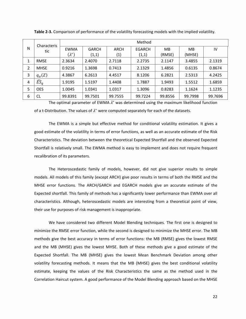
Table 2‐3. Comparison of performance of the volatility forecasting models with the implied volatility.
N Characteris
tic
Method
EWMA
GARCH (1,1)
ARCH (1)
EGARCH (1,1)
MB (RMSE)
MB (MHSE)
IV
1 RMSE 2.3634 2.4070 2.7118 2.2735 2.1147 3.4855 2.1319
2 MHSE 0.9216 1.3698 0.7413 2.1329 1.4856 0.6135 0.8674
3 4.3867 6.2613 4.4517 8.1206 6.2821 2.5313 4.2425
4 1.9195 1.5197 1.4408 1.7887 1.9493 1.5512 1.6859
5 OES 1.0045 1.0341 1.0317 1.3096 0.8283 1.1624 1.1235
6 CL 99.8391 99.7501 99.7555 99.7224 99.8556 99.7998 99.7696 The optimal parameter of EWMA was determined using the maximum likelihood function
of a t‐Distribution. The values of were computed separately for each of the datasets.
The EWMA is a simple but effective method for conditional volatility estimation. It gives a
good estimate of the volatility in terms of error functions, as well as an accurate estimate of the Risk
Characteristics. The deviation between the theoretical Expected Shortfall and the observed Expected
Shortfall is relatively small. The EWMA method is easy to implement and does not require frequent
recalibration of its parameters.
The Heteroscedastic family of models, however, did not give superior results to simple
models. All models of this family (except ARCH) give poor results in terms of both the RMSE and the
MHSE error functions. The ARCH/GARCH and EGARCH models give an accurate estimate of the
Expected shortfall. This family of methods has a significantly lower performance than EWMA over all
characteristics. Although, heteroscedastic models are interesting from a theoretical point of view,
their use for purposes of risk management is inappropriate.
We have considered two different Model Blending techniques. The first one is designed to
minimize the RMSE error function, while the second is designed to minimize the MHSE error. The MB
methods give the best accuracy in terms of error functions: the MB (RMSE) gives the lowest RMSE
and the MB (MHSE) gives the lowest MHSE. Both of these methods give a good estimate of the
Expected Shortfall. The MB (MHSE) gives the lowest Mean Benchmark Deviation among other
volatility forecasting methods. It means that the MB (MHSE) gives the best conditional volatility
estimate, keeping the values of the Risk Characteristics the same as the method used in the
Correlation Haircut system. A good performance of the Model Blending approach based on the MHSE

23
error function has shown that, the MHSE error has an advantage over the RMSE for the problems of
the conditional volatility estimation. We can conclude that a method which will give a low MHSE
error most probably will also produce suitable values of the Risk Characteristics. The main
disadvantage of the Model Blending approach is that it requires the implementation and calibration
not of one model but of all the models used in blending. The parameter calibration procedure is
complicated and could potentially require repeated recalibration of the parameters. The MB method
is a “black‐box” approach; the forecasts made by this method are often non‐intuitive.
We have compared the results of the Historical volatility models with the Implied Volatility
approach. The results are represented in Table 2‐3. We would like to stress that those results are less
reliable, because the comparison was made only for a limited number of financial products. For the
selected products the IV gives low values of error functions as well as a good estimate of the Risk
Characteristics. The IV estimates volatility based on the market values of the options. This connection
with the market makes IV an attractive technique. The main disadvantage of this method is that on
average it tends to overestimate the observed volatility. Implied volatility reflects the ‘fears’ of
market players. Another disadvantage is that for some assets this method is hard to implement as
there are no options traded or the traded options are not liquid.
We have compared several popular methods for the conditional volatility estimation. Each
method has its advantages and disadvantages, which were described in this chapter. Some methods
are simple but yield poor results, while other methods provide improved results but are difficult to
implement. In short there is no perfect approach. The Exponentially Weighted Moving Average
method with the optimal set of parameters provides good results in terms of both error functions
and Risk Characteristics. Although some methods (MB‐MHSE) outperform EWMA, the EWMA method
is easy to implement and to calibrate. The Implied Volatility can be also successfully used as a
volatility estimation technique for the liquid assets. We can conclude that the combination of EWMA
and IV approach should be used for purposes of risk management.

24
3 Modeling implied volatility surfaces
3.1 Risk of volatility “smile” and its impact European options are often priced or hedged using the Black‐Scholes model (Black & Scholes,
1973). The model gives an one‐to‐one relationship between the price of the European put or call
option and the implied volatility. It assumes that the price of the underlying asset follows the
geometric Brownian motion with constant volatility. This is a rather crude assumption, because it
implies that the volatility parameter is equal for all the strikes. The Black‐Scholes conditions never
hold exactly in the markets. This happens due to different factors, for example, jumps in underlying
asset prices, movements of volatility over time, transaction costs, etc. Therefore, practitioners often
use different values of implied volatility for different strike prices. This forms a specific pattern, called
the “implied volatility smile”. Although, this pattern could be in a form of a “skew”, ”smile” or a
“sneer”, we will refer to it as a “skew”. The implied volatility surface is a more general representation
of implied volatility smile pattern. By the implied volatility surface we will understand the
dependence between the price of the underlying asset, strike price of the option, time to maturity of
the option and its implied volatility.
Changes of the implied volatility have a significant influence on the value of the option
position. An incorrect estimate of the implied volatility and its expected shifts could lead to a
significant miss‐pricing of the options. That is why modeling the implied volatility surfaces plays an
important role in financial risk management. In this section we will test several models for implied
volatility surface modeling. We will include different types of polynomial fitting as well as a stochastic
volatility models in our analysis.

25
3.2 Representation of the moneyness The volatility skew or surface is usually expressed in terms of moneyness rather than in
terms of a simple strike price . Moneyness is a ratio between the strike price and the price of the
underlying asset . We will focus on two different representations of moneyness. The first
representation of moneyness is given by the following equation:
/ . (3.1)
Alternatively, we can formulate moneyness in terms of time to expiration. Let us denote time to
expiration as , where ‐ is a date of expiration of a given option and is a current date.
Then the moneyness can be redefined as:
/
√. (3.2)
An option is said to be at‐the‐money if 0. A call (put) option is said to be in‐the‐money (out‐of‐
the‐money) for 0 and out‐of‐the‐money (in‐the‐money) for 0. The comparison of the
volatility skew for different moneyness is represented in Figure 3‐1.
Figure 3‐1: The observed implied volatility of the AEX index options on 24‐10‐2007. Left: representation in the log‐
moneyness (3.1). Right: representation in the time adjusted moneyness (3.2). Different colors represent different time‐
to‐expiration in days.
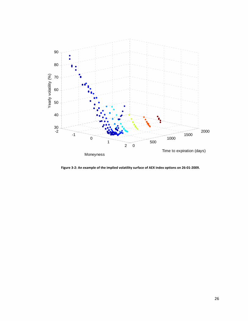
The implied volatility surface is the representation of the implied volatility as a function of
moneyness and time to expiration , . An example of the volatility surface is given in
Figure 3‐2.
-0.6 -0.4 -0.2 0 0.2 0.415
20
25
30
35
Moneyness
Vol
atili
ty (%
)
-0.6 -0.4 -0.2 0 0.2 0.415
20
25
30
35
Time-adjusted moneyness
Vol
atili
ty (%
)
200
400
600
800
1000
1200
1400
200
400
600
800
1000
1200
1400
26
Figure 3‐2: An example of the implied volatility surface of AEX index options on 26‐01‐2009.
-2-1
01
2 0500
10001500
200030
40
50
60
70
80
90
Time to expiration (days)Moneyness
Yea
rly v
olat
ility
(%)

27
3.3 Models of the implied volatility surface There are a number of mathematical models that describe the implied volatility surfaces. An
overview of some of them will be given in this chapter. We will focus on the models which are
extensively described in the literature and have a proven record of effectiveness.
We will start our overview with the polynomial models. The Cubic model is a model for
volatility surfaces. It uses the time adjusted form of moneyness (3.2). This model treats the implied
volatility as a cubic function of moneyness and a quadratic function of the time to expiration . The
model is described by the following equation:
, (3.3)
Parameters , , , , and are estimated using the least squares method. The Cubic model
describes whole volatility surface with one equation.
Figure 3‐3: An example of the fit of the Cubic model to the AEX index options implied volatility surface on 26‐01‐
2009.
-2-1
01
2 0500
10001500
200020
30
40
50
60
70
80
90
Time to expiration (days)Moneyness
Yea
rly v
olat
ility
(%)
Observed volatilityCubic model

28
So for any given moneyness and time to expiration one can find the value of implied
volatility.This model is a smooth function of moneyness and time to expiry. An example of the fit of
the cubic surface model is given in Error! Reference source not found..
With the analogies to the Cubic model, we can build a Spline model of the volatility surface.
We are using the time adjusted form of moneyness (3.2). Let us introduce the dummy variable :
0, 0,1, 0. (3.4)
The volatility function is given by:
.
(3.5)
We would like the function of volatility to be continuous and differentiable. This is achieved by
adding the following constrains:
· 0 · 0 0, (3.6)
0. (3.7)
We get the following function of the implied volatility, after rearranging the terms of (3.5):
.. (3.8)
The parameters , , , , and are fitted using the linear least squares regression analysis.
The whole volatility surface is described by six parameters. The Spline model gives a value of the
volatility for any value of , and does not require any additional interpolation over the time to
expiration. An example of the fit of this model is given in Figure 3‐4.

29
Figure 3‐4: An example of the fit of the Spline model to the volatility surface of AEX index options on 26‐11‐2008.
The Stochastic alpha, beta, rho (SABR) is another important class of volatility models. The
SABR model was introduced in 2002 (Hagan, Kumar, Lesniewski, & Woodward, 2002). This model
assumes some behavior of the underlying asset and connections with the values of the implied
volatility. The shape of the volatility skew is derived analytically from these assumptions. Let us
denote the today’s forward price of the underlying asset by and the forward price of the asset for a
forward contract that matures on the fixed settlement date by . Today’s forward price is defined
as 0 . The strike price of an European option is denoted by . The forward price and the
volatility are described by the following processes:
, 0 , (3.9)
, ̂ 0 , (3.8)
under the forward measure, where the two processes are correlated by :
-3-2
-10
12 0
5001000
150030
40
50
60
70
80
90
100
110
Time to expiration (days)Moneyness
Yea
rly v
olat
ility
(%)
Observed volatilitySpline model
30
, (3.11)
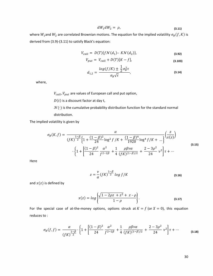
where and are correlated Brownian motions. The equation for the implied volatility , is
derived from (3.9)‐(3.11) to satisfy Black’s equation:
– , (3.92)
, (3.103)
,
/ 12
√, (3.14)
where,
, are values of European call and put option,
is a discount factor at day t,
· is the cumulative probability distribution function for the standard normal
distribution.
The implied volatility is given by
, 1 1
24 log / 11920 log / …
· 1124
14 /
2 324
(3.15)
Here
/ (3.16)
and is defined by
1 2 –
1. (3.17)
For the special case of at‐the‐money options, options struck at (or 0), this equation
reduces to :
, · 1124
14 /
2 324
(3.18)
31
The detailed description and derivation of equations (3.15)‐(3.18) can be found in (Hagan, Kumar,
Lesniewski, & Woodward, 2002). The SABR model can be easily rewritten to take relative strikes
(moneyness) as input. In this case:
, 1 , . (3.19)
There is a special procedure for calibrating the parameters of the SABR model. We will start
with the parameter. (Hagan, Kumar, Lesniewski, & Woodward, 2002) and (Poon S. , 2008) suggest
to fix the parameter in advance and not to change it. There are two special cases: 0 and
1. The first one represents a stochastic normal model, while the second one ( 1) represents a
stochastic log‐normal model. The value of should be chosen to be between 0 1. We will focus
on the case of 1. Once is fixed, all other parameters can be adjusted to the value of the .The
particular value of has little impact on the shape of the implied volatility skew. This parameter can
be successfully chosen from “esthetical” considerations (West, 2005).
The parameter refers to the value of the at‐the‐money volatility. There are two ways of estimating
this parameter. It could be taken as a value of at‐the‐money volatility . Or it could be
estimated as a smallest positive solution of the following equation:
124
14
12 324
0. (3.11)
The parameter should chosen to be positive, 0. Changes of the parameter shift the implied
volatility skew across the volatility axis. It controls the level of the implied volatility curve or surface.
The parameters and are calibrated to minimize the error between the observed implied
volatilities and the SABR model (3.15)‐(3.17). The parameter refers to the volatility of the implied
volatility and is called ‘volvol’. The parameter is a correlation coefficient between the at‐the‐money
volatility and movements of the underlying asset. To calibrate and the two dimensional Nelder‐
Mead algorithm was suggested by (West, 2005). The algorithm gives the optimal values and
that minimize the quadratic error:
, min , – , , (3.12)
where,

32
, 1, … , are the values of the implied volatility obtained from the market
prices of the options,
, 1, … , are the SABR estimations of the implied volatility.
Now, we can summarize the procedure of fitting the parameters of the SABR model. Firstly, fix the
value of parameter. We are taking 1 in all of our experiments. Secondly, find the value of .
This can be done by solving (3.11) or by fixing . For practical reasons, we will fix to be
equal to the volatility of at‐the‐money options. At last, the parameters and are calibrated using
procedure (3.12). All the remaining parameters of the SABR equation (3.15)‐(3.17) are known for a
given contract. Although, (3.15)‐(3.17) looks complicated, it involves only simple mathematical
operations and can be implemented rather easily.
The SABR model can be used as a model for a whole volatility surface or for the skew
(fixed ). We will discuss these two approaches separately. Under the first approach, the parameters
, , , are calibrated for all given times to expiration , 1, … , . A point on the volatility
surface is obtained by applying (3.15)‐(3.17). An example of the SABR volatility is given in Figure 3‐.

33
Figure 3‐5: An example of the fit of the SABR model to the volatility surface of AEX index options on 9‐7‐2008.
A second approach is to fit a SABR skew for each observed time to expiration. And then
interpolate the values of implied volatility for any arbitrary . The SABR parameters , , ,
are calculated separately for each time to expiration , 1, . . , . The implied volatility surface is
built as a linear approximation of separate skews.
, , , ,––
, ,–
. (3.13)
where,
is the value of the implied volatility for any arbitrary time to expiration
, are values of the implied volatility calculated from time to expiration that are
observed on the market , .
We will refer to this method as piecewise SABR (PSABR). An example of the fit of the PSABR is given
in Figure 3‐.
-1.5 -1 -0.5 0 0.5 1 1.50
1000
2000
15
20
25
30
35
40
45
50
55
Time to expiration (days)
Moneyness
Yea
rly v
olat
ility
(%)
Observed volatilitySABR model

34
Figure 3‐6: An example of the fit of the PSABR model to the observed implied volatility skew of the AEX index
options on 17‐3‐2008, with time‐to‐expiration of 95 days.
-0.4 -0.2 0 0.2 0.4 0.6 0.8 120
22
24
26
28
30
32
34
36
38
Moneyness
Yea
rly v
olat
ility
(%)
Observed volatilityPSABR model
35
3.4 Modeling the dynamics of volatility surfaces The value of the implied volatilities changes with time, deforming the shape of the implied
volatility surface. The evolution in time of this surface captures the changes in the options market.
While a model with a large number of parameters may calibrate well the volatility surface on a given
day, the same model parameters may give poor result on the next day. Any risk management system
tries to estimate the future (short term forecast) behavior of the volatility surface. Modeling the
dynamics of the implied volatility surface is an important task from practical point of view. In this
chapter we will discuss different techniques to model the dynamics of the implied volatility surfaces.
We will focus on two different approaches. One will be applicable to the cubic and the spline model;
the other will be used for SABR models.
The Cubic (3.3) and the Spline (3.8) models of the volatility surface use parameters
, 1, . . , to model the shape of the surface. The dynamics of the surface is treated as dynamics
of these parameters. So, we can assume that , 1, … , . In order to reduce the
dimensionality of the problem, we apply Principal Component Analysis (PCA) to the values of
, 1, … , . The PCA is a statistical technique widely used in practice as a preprocessing technique.
The details of the PCA could be found in (Shlens, 2005). Let us denote by matrix ; the matrix
of observations of coefficients , 1, … , ; 1, … , of the implied volatility surface. After
applying PCA to the matrix , we will obtain the matrixes , and a vector . is a matrix,
each column containing coefficients for one principal component. The columns are in order of
decreasing component variance. is an matrix, the representation of in the principal
component space. is a vector containing the eigenvalues of the covariance matrix of . An example
of is given on Figure 3‐. PCA is theoretically the optimal linear scheme, in terms of least mean
squares error, for compressing a set of highly‐dimensional vectors to a set of lower‐dimensional
vectors and then reconstructing the original set (Shlens, 2005). Working with coefficients of the
models (3.3), (3.8) can be substituted by working with the matrix . Moreover, the first few principal
components explain most of the variance of the A. For practical considerations we will focus on the
first two principal components. The dynamics of the volatility surface over time is explained by
dynamics of these two variables. An example of the dynamics of the first and the second principal
component is given in Figure 3‐.

36
Figure 3‐7: A PCA of the coefficients of the Cubic model of the fit of AEX index implied volatility surface. The first two
components explain almost all variance of the coefficients.
Figure 3‐8: The dynamics of the 1st and the 2nd principal component of the coefficients of the Cubic model for the
AEX index implied volatility.
0 1 2 3 4 5 6 70
20
40
60
80
100
Principal Component
Var
ianc
e E
xpla
ined
(%)
Jun 2007 Jan 2008 Aug 2008 Apr 2009-50
0
50
100
Firs
t Prin
cipa
l Com
pone
nt
Jun 2007 Jan 2008 Aug 2008 Apr 2009-60
-40
-20
0
20
40
Sec
ond
Prin
cipa
l Com
pone
nt

37
We assume that the two first principal components and have a significant value of sample
partial autocorrelation. A sample partial autocorrelation function for the first two principal
components is given in Figure 3‐.
Figure 3‐9: A sample partial autocorrelation function of the 1st and the 2nd principal components of the Cubic model
applied to the AEX index implied volatility surface. Both, the 1st and the 2nd principal component exhibit a significant
value of the autocorrelation for a 1 day lag.
The dynamics of and can be modeled with an Autoregressive moving average model
(ARMA):
̂ 1 1 , (3.14)
where , , … , and , , … , are parameters of the model and , , … , are the error
terms of the model ̂ . We will refer to this model as the ARMA(p,q) model. For a
particular case of modeling and , we will take 1 and 1. The parameters and
are estimated using a least squares method.
Now, we can summarize the procedure of modeling the dynamics of the implied volatility
surface for cubic and spline models. First, we apply the PCA to the historical observations of
, 1, … , .to obtain observations of and . Then the ARMA model (3.14) is calibrated
and applied to get the forecast ̂ 1 and ̂ 1 . After that, the PCA is applied “backwards”
0 5 10-0.2
0
0.2
0.4
0.6
0.8
Lag
Sam
ple
Par
tial A
utoc
orre
latio
ns
Sample Partial Autocorrelation FunctionFirst Principal Component
0 5 10-0.2
0
0.2
0.4
0.6
0.8
Lag
Sam
ple
Par
tial A
utoc
orre
latio
ns
Sample Partial Autocorrelation FunctionSecond Principal Component

38
(Shlens, 2005) to construct the forecast of 1 , 1, … , . The forecasted surface is
constructed from 1 , 1, … , using Error! Reference source not found. or (3.8). The
rincipal Component Analysis is a popular statistical technique to reduce the dimensionality of the
problem. We are using PCA in a somewhat nonstandard way. We are reducing the relatively small
number of variables (coefficients of a Spline or Cubic model) even more. The main reason for the PCA
for our problem is to switch to another space of the no‐correlated factors, that fully describe the
dynamic of the implied volatility surface.
Apart from the previously discussed model of dynamics, the SABR model already assumes
certain dynamics of the volatility and the underlying asset. This dynamics is expressed by a system of
stochastic differential equations:
, 0 , (3.24)
, ̂ 0 , (3.25)
where and are correlated Brownian motions
. (3.26)
Instead of the forward price of the underlying asset , the current spot price of the underlying asset
can be used. Suppose, the SABR model is already calibrated and parameters , , , are already
known. Then (3.24)‐(3.26) can be simulated with the Monte‐Carlo method (MC). (3.24)‐(3.26) are
model dependent on random variables (changes of Brownian motion). Under the MC method we
assume some distribution of these random variables and generate realizations of them. Based
on these realizations we calculate outputs of the model. The average of the outputs is used as a
forecast of the process. In our particular case, the change of Brownian motion has a normal
distribution ~ 0,1 , 1,2 . We will use the following approach in order to generate
correlated random numbers with a correlation coefficient . First, we generate two
uncorrelated sequences of normal random numbers , . The correlated sequence of random
numbers is constructed in the following way:
1 . (3.27)
The sample paths of the underlying asset and volatility‐like parameter are generated from (3.24)
and (3.25). The SABR equations (3.15)‐(3.17) are applied for each path of the MC simulation. This
39
results to the simulated implied volatility surfaces. The forecast of the implied volatility surface
is an average surface over the simulated paths.
We should note that the forecasting procedure is slightly different for the SABR surface
model than for the PSABR model. The SABR surface is described by 4 parameters , , and . The
forecasting algorithm is the same as described earlier. But the PSABR model is described by 4
parameters, where is a number of is is different time to expiry in the observed option portfolio.
The dynamics of each volatility skew (fixed ) is considered to be a separate process. The MC
simulation is applied separately for each of the sets of parameters. This will lead to the
forecasted implied volatility skews. The implied volatility surface is constructed from these skews by
applying (3.13).
The Sticky‐Strike rule is another approach which is used for estimating the shifts of the
implied volatility. The main idea is the assumption that if the price of the underlying asset changes,
than the implied volatility of an option with a given strike does not change. The Sticky‐Strike rule is
very popular among practitioners, because it easy to understand and does not require complex
computations. Let us formalize this approach. The Sticky‐Strike rule suggests that:
, , , 1 , 1 , (3.28)
where
, 1 , 1 is the value of the implied volatility on a day 1,
, , is the value of the implied volatility on a day , for the same strike .
The Sticky‐Strike rule is not a model of the implied volatility surface. It does not provide an equation
which can give a value of volatility for any strike, moneyness or time to expiration. It is only an
empirical rule to estimate the future behavior of the implied volatility of the options in a given
portfolio.

40
3.5 Comparison of the volatility surface models The models and methods described in the previous chapters were tested on market data, in
order to determine their advantages and disadvantages. The testing data consists of 10 separate sets,
each corresponding to a different underlying asset. The list of data sets with a short description is
given in Table 3‐1.
Table 3‐1. The characteristics of the data sets used for the analysis.
N Underlying symbol
Description Dates of observations Number of days
Adjusted for implied
dividends (Y/N) 1 AEX Amsterdam Stock Index 7‐6‐2007 to 1‐ 4‐2009 467 Y 2 DAX German Stock Index 7‐6‐2007 to 11‐5‐2009 496 Y 3 FTSE UK Stock Index 7‐6‐2007 to 11‐5‐2009 494 Y 4 EURSTOX European Stock Index 7‐6‐2007 to 11‐5‐2009 494 Y 5 S&P 500 US Stock Index 7‐6‐2007 to 11‐5‐2009 486 Y 6 XJO Australian Stock Index 7‐6‐2007 to 11‐5‐2009 499 N 7 DBK Deutsche Bank Stock 7‐6‐2007 to 11‐5‐2009 494 N 8 VOW Volkswagen Stock 7‐6‐2007 to 11‐5‐2009 494 N 9 ALV Allianz Stock 7‐6‐2007 to 11‐5‐2009 494 N 10 ADS Adidas Stock 7‐6‐2007 to 11‐5‐2009 494 N
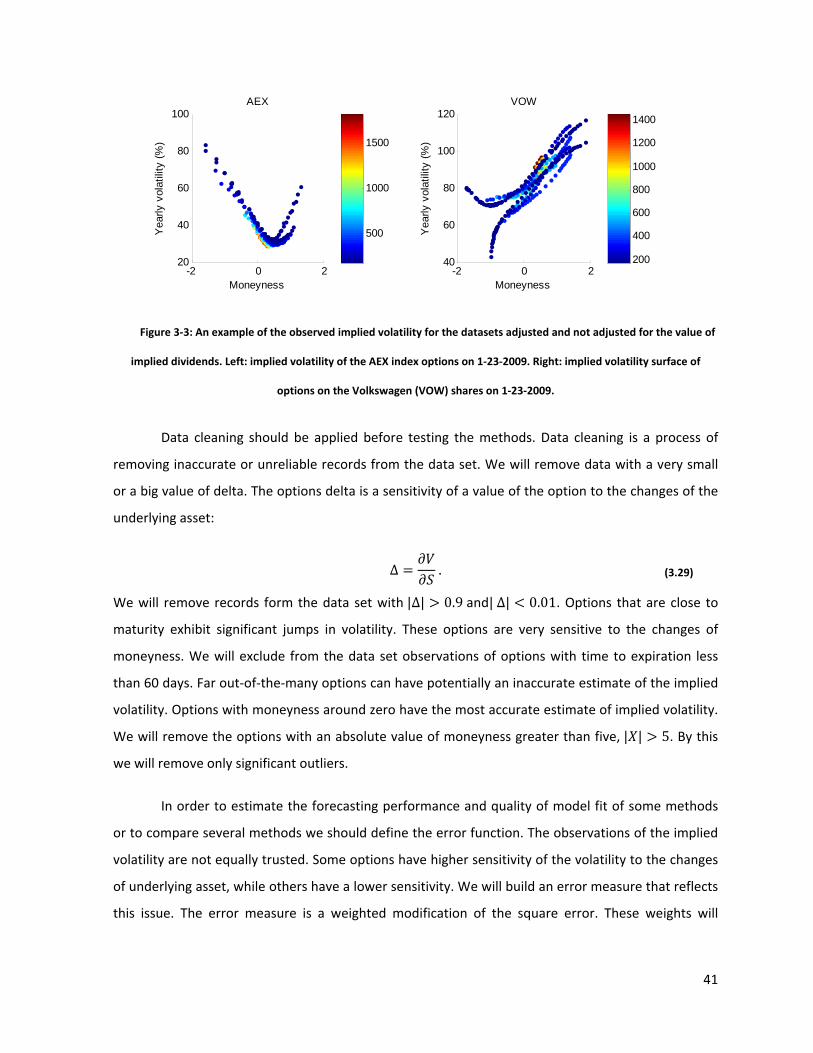
The data set includes the values of implied volatilities of put and call options with different
time to expiration. Each record is characterized by date of trade, strike price, price of the underlying
asset, time to expiration, implied volatility (derived from the market price of the option) and type of
the option (put or call). Put –call parity (Hull, 2002) suggests that implied volatilities of call options
should not significantly deviate from the implied volatilities of the put options for the same
moneyness. However, in practical applications this deviation is commonly observed. The adjustment
for implied dividends of the underlying asset can be made, in order to eliminate these deviations
(Hafner & Wallmeier, 2000). Part of the data set is adjusted for the value of the implied dividends. As
a result, the values of the implied volatility for call and put options are almost equal. This adjustment
is mainly done when the underlying asset is a stock index (see Table 3‐1). The other part of the data is
not adjusted for the value of implied dividends. An example of the implied volatility skew with and
without adjustment is given in Figure 3‐3.
41
Figure 3‐3: An example of the observed implied volatility for the datasets adjusted and not adjusted for the value of
implied dividends. Left: implied volatility of the AEX index options on 1‐23‐2009. Right: implied volatility surface of
options on the Volkswagen (VOW) shares on 1‐23‐2009.
Data cleaning should be applied before testing the methods. Data cleaning is a process of
removing inaccurate or unreliable records from the data set. We will remove data with a very small
or a big value of delta. The options delta is a sensitivity of a value of the option to the changes of the
underlying asset:
Δ . (3.29)
We will remove records form the data set with |Δ| 0.9 and| Δ| 0.01. Options that are close to
maturity exhibit significant jumps in volatility. These options are very sensitive to the changes of
moneyness. We will exclude from the data set observations of options with time to expiration less
than 60 days. Far out‐of‐the‐many options can have potentially an inaccurate estimate of the implied
volatility. Options with moneyness around zero have the most accurate estimate of implied volatility.
We will remove the options with an absolute value of moneyness greater than five, | | 5. By this
we will remove only significant outliers.
In order to estimate the forecasting performance and quality of model fit of some methods
or to compare several methods we should define the error function. The observations of the implied
volatility are not equally trusted. Some options have higher sensitivity of the volatility to the changes
of underlying asset, while others have a lower sensitivity. We will build an error measure that reflects
this issue. The error measure is a weighted modification of the square error. These weights will
-2 0 220
40
60
80
100
Moneyness
Yea
rly v
olat
ility
(%)
AEX
-2 0 240
60
80
100
120
Moneyness
Yea
rly v
olat
ility
(%)
VOW
200
400
600
800
1000
1200
1400
500
1000
1500
42
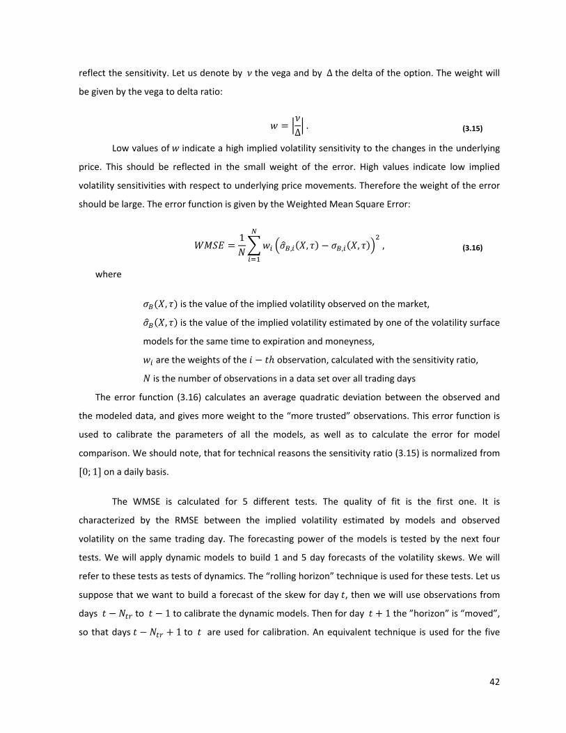
reflect the sensitivity. Let us denote by the vega and by Δ the delta of the option. The weight will
be given by the vega to delta ratio:
Δ. (3.15)
Low values of indicate a high implied volatility sensitivity to the changes in the underlying
price. This should be reflected in the small weight of the error. High values indicate low implied
volatility sensitivities with respect to underlying price movements. Therefore the weight of the error
should be large. The error function is given by the Weighted Mean Square Error:
1
, , , , , (3.16)
where
, is the value of the implied volatility observed on the market,
, is the value of the implied volatility estimated by one of the volatility surface
models for the same time to expiration and moneyness,
are the weights of the observation, calculated with the sensitivity ratio,
is the number of observations in a data set over all trading days
The error function (3.16) calculates an average quadratic deviation between the observed and
the modeled data, and gives more weight to the “more trusted” observations. This error function is
used to calibrate the parameters of all the models, as well as to calculate the error for model
comparison. We should note, that for technical reasons the sensitivity ratio (3.15) is normalized from
0; 1 on a daily basis.
The WMSE is calculated for 5 different tests. The quality of fit is the first one. It is
characterized by the RMSE between the implied volatility estimated by models and observed
volatility on the same trading day. The forecasting power of the models is tested by the next four
tests. We will apply dynamic models to build 1 and 5 day forecasts of the volatility skews. We will
refer to these tests as tests of dynamics. The “rolling horizon” technique is used for these tests. Let us
suppose that we want to build a forecast of the skew for day , then we will use observations from
days to 1 to calibrate the dynamic models. Then for day 1 the ”horizon” is “moved”,
so that days 1 to are used for calibration. An equivalent technique is used for the five

43
days ahead forecast. In practical applications we will take 100. The remaining two tests are
applied to check how the models can “hold” the volatility skew pattern. The WMSE is calculated
between the model results and observed implied volatility on day , similar to the quality of fit test.
But, in this case the parameters of the models are calibrated on observations of day 1 or 5.
We will refer to these tests as “static tests”. The averaged WMSE of the models over data sets
adjusted for the value of implied dividends is given in Table 3‐2.The results of the test for the
remaining data sets is given in Table 3‐3. The WMSE for each of the underlying assets is given in
section 5.5.
Table 3‐2. Averaged results of the tests for the following underlying assets: AEX, DAX, FTSE, EUROSTOXX, and S&P500.
N Model Quality of
fit
Static models Dynamic models 1 day
forecast 5 days forecast
1 day forecast
5 days forecast
1 Cubic 0.82596 2.44567 5.37869 2.78673 7.89823 2 Spline 0.63001 1.97957 4.65466 2.53439 6.47271 3 SABR 4.22855 5.11622 7.82890 5.11794 7.32580 4 PSABR 2.32145 3.27966 5.88138 4.50680 6.70848 5 Sticky Strike N/A 1.23520 3.02228 N/A N/A Table 3‐3. Averaged results of the tests for the following underlying assets: XJO, DBK, VOW, ALV and ADS.
N Model Quality of
fit
Static models Dynamic models 1 day
forecast 5 days forecast
1 day forecast
5 days forecast
1 Cubic 4.16422 10.60288 22.37566 18.72404 50.34940 2 Spline 3.94045 9.54097 20.81255 12.61659 34.76029 3 SABR 14.20002 21.10567 38.06475 21.11537 33.90157 4 PSABR 5.47680 11.14137 23.03782 13.04728 23.03009 5 Sticky Strike N/A 7.42659 16.40627 N/A N/A
We can shortly summarize the advantages of each model, given the results of the tests. The
Cubic and Spline models approximate the implied volatility surface with the function of a certain
form. On average, the Spline model performs better than the Cubic model. Good performance of the
dynamic version of the Spline model is an empirical evidence of the dependence of the dynamics of
the surface of two principal components. Both of these models use much less parameters, than the
PSABR model. Both of these models use much less parameters, than the PSABR model. Spline and
Cubic model use one set of parameters to approximate whole surface, while PSABR use a separate
set of parameters for each skew (which corresponding to fixed time to expiry).

44
The SABR and the PSABR assume a certain model for the joint dynamics of the volatility and
the underlying asset. Unfortunately, the SABR model gives a higher error than other models. The
PSABR model gives much better results. Although, the PSABR does not give the best forecast, it
models the skew rather effectively, in case of insufficient or “bad” data. The SABR family of models
assumes some shape (“skew”, ”smile”, “sneer”, etc.) of the volatility skew and fits it to the given data.
The SABR gives a more “theoretical” shape of the skew. This results to a higher fitting error, but lower
relative forecasting error (error of forecast divided by the error of fit). Another advantage of the SABR
model is that each parameter has a certain meaning. The parameter is a correlation between the
changes of at‐the‐money volatility and the underlying asset, is so‐called “volvol” the volatility of the
volatility, and is associated with at‐the‐money volatility. These values are a useful
“complementary” product of the SABR model, and can be used in other applications of risk
management.
The Sticky Strike rule is a simple, but very effective way to estimate the shifts of the implied
volatility. The WMSE of this method is one of the lowest over all data sets. The main disadvantage of
this method is that it estimates the implied volatility only of those options that are being
continuously tracked. In practical applications, however, not all the options are tracked to compute
the implied volatility. Usually, the limited portfolio is considered; it makes it impossible to apply the
Sticky Strike rule for any strike, moneyness and time to expiry. The sticky Strike is simple method; it
does not require any computations or parameter estimates and can be effectively used as a
complementary method.
Modeling the implied volatility surface is a challenging task. In this work we have tried several
methods and approaches to solve this problem. We have developed and tested a number of models.
We have demonstrated that there is no single model, which significantly outperforms the other. Each
model has its advantages and disadvantages. The Spline model is perhaps, the most effective to
minimize the fitting error. The SABR model has a set of meaningful parameters and a more significant
“forecasting power” It performs better on an incomplete or missing data.

45
4 Conclusions and practical recommendations This project is dedicated to addressing the problem of volatility modeling in financial markets.
We focused on two major aspects of the volatility problem: the conditional volatility estimation and
modeling volatility surfaces. The volatility modeling problem was studied with the purposes of
financial risk management.
The first part of this thesis deals with the problem of conditional volatility estimation. We
have selected several methods that are heavily used in practice and tested their accuracy using a
number of different classes of real data. Each family of methods has its advantages and
disadvantages, which are described in this work. Some methods yield poor results (e.g., the
heteroscedastic family of models), while the others provide improved results but are difficult to
implement (e.g., models blending). In short, there is no single perfect approach. Nevertheless, we
found that the Exponentially Weighted Moving Average method is efficient and is relatively easy to
implement. We have described the procedure to calibrate the parameters of this model. We have
also tested Model Blending techniques. This is a relatively new approach, and we confirmed that it
can be successfully used for volatility forecasting. The Model Blending approach certainly provides a
superior accuracy over other methods. Its practical application, however, is compromised by an
extremely complex procedure of parameter calibration. Given all these considerations, we suggest
the following recommendations for conditional volatility estimation: a combination of the EWMA
model (with properly calibrated parameters) and the Implied Volatility method.
The second part of this project is dedicated to modeling of implied volatility surface. We have
studied two major classes of the volatility skews: the polynomial models (e.g., Cubic, Spline etc.) and
stochastic models (the SABR model). Special attention was paid to the problems of the dynamics of
the implied volatility surface in time. All of the models were tested on market data, which included
different classes of underlying assets as well as different markets. We have suggested and applied
different tests to compare implied volatility surface models. We have described the advantages and
disadvantages of each method. We demonstrate that no single method exhibits superior accuracy in
the analysis of every data set. Some methods perform better for certain underlying assets, while
other methods are more suitable for the other.

46
5 Appendixes
5.1 t LocationScale distribution In this appendix we will discuss the t Location‐Scale distribution, its likelihood function and
the results of fitting the distribution to the returns of the datasets of Section 2.5.
The t Location‐Scale distribution is a continuous distribution with the following density
function:
Γ 1
2√ Γ 2
, (5.1)
where
Γ ‐ gamma function,
– shape parameter of the distribution,
‐ location parameter of the distribution,
0 – scale parameter.
If a random variable has a t Location‐Scale distribution, with parameters , and ,
then the following random variable
,
will have a Student’s t distribution with degrees of freedom.
The likelihood function of the t Location‐Scale distribution is given by the following equation:
, | , (5.2)
where
‐ density function of a t Location‐Scale distribution,
, , ‐ parameters of the t Location‐Scale distribution.
Values of parameters of t Location‐Scale distribution for the testing datasets are given in
Table 5‐1.
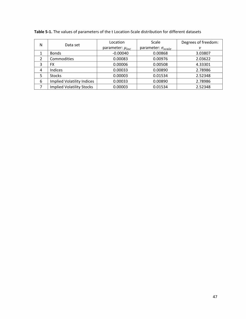
47
Table 5‐1. The values of parameters of the t Location‐Scale distribution for different datasets
N Data set Location
parameter: Scale
parameter: Degrees of freedom:
1 Bonds ‐0.00040 0.00868 3.03807 2 Commodities 0.00083 0.00976 2.03622 3 FX 0.00006 0.00508 4.33301 4 Indices 0.00033 0.00890 2.78986 5 Stocks 0.00003 0.01534 2.52348 6 Implied Volatility Indices 0.00033 0.00890 2.78986 7 Implied Volatility Stocks 0.00003 0.01534 2.52348

48
5.2 The BlackScholes option pricing equation In this appendix we introduce some definitions and give the Black‐Scholes equation for option
pricing.
An European call option is a financial contract that gives the holder the right but not the
obligation to buy an underlying asset at a certain date (expiry date) for a certain price (exercise or
strike price). European put option, unlike the call option, gives to its holder the right to sell an
underlying asset at a certain date for a certain price.
In early 1970s, Fischer Black, Myron Scholes and Robert Merton made a major breakthrough
into stock option pricing. This involved the development of what became known as the Black‐Scholes
model. In 1997 Myron Scholes and Robert Merton received a Nobel Prize in economics for their
contribution in derivatives pricing. Let us introduce the assumptions and some important results of
this model. The original assumptions are:
• The underlying stock price ( ) is described by the following process:
where is expected rate of return (the drift), is the constant
volatility of the returns, is a Brownian Motion.
• There are no transaction costs and all securities are perfectly divisible.
• There are no arbitrage opportunities.
• The risk free interest rate, , is constant and the same for all maturities. Investors can
freely borrow and lend money for the risk free interest rate.
The assumptions of the Black‐Scholes model are rather strong and unrealistic. Extensions of the
Black‐Scholes model manage to overcome most of these restrictions. Still the assumption of constant
volatility is one of the strongest.
Let us denote price of a European call option as , European put and strike price. Then
and can be found by the following equations:
, (5.3)
, (5.4)
where,

49
ln ⁄ 2⁄
√,
√ ,
- is the cumulative probability distribution function for standard normal distribution,
‐ is the price of underlying asset at time 0,
- is the expected dividend rate.

50
5.3 Cross validation In this appendix we discuss questions of dividing the data set into the subsets for validation of
the results. Cross‐validation is, probably, the simplest and the most effective method to estimate a
prediction error on a data set (Hastie, Tibshirani, & Friedman, 2002). The main idea of this method is
to divide the data set into several sub‐parts, and to use some of them as a training set and others as a
testing set. The training set is a part of all available data which is used to calibrate the models of
interest, while the testing set is used to calculate the error.
The fold cross‐validation could be described by the following algorithm. In the first step all
available data is divided randomly into equal parts (folds). So in each fold we have data which
corresponds to different time periods. Then the 1st fold is used as a testing set and the remaining
1 folds are used as a training set. In the next step the 2nd fold is used as a testing set and the
remaining folds (including the 1st one) are used as a training set. The algorithm is repeated on folds.
We will obtain values of error; the resulting error is the average of these values. We will take
5 for practical considerations.
The main advantage of the cross‐validation technique is that the outliers and special
observations will be equally distributed between the training and testing subsets. This is especially
important for the problems of volatility estimation, because high values of volatility tend to cluster. If
a certain model will be calibrated only on a low volatility period it will most probably fail to correctly
estimate volatility on a high volatility testing set.

51
5.4 Results of the conditional volatility estimation In this section we will present detailed results of the empirical tests of the volatility forecasting
models discussed in Section 2.5. We will use the following notation for the characteristics of tests:
1. RMSE – Root Mean Square Error, see (2.11)
2. MHSE – Mean Heteroscedastic error , see (2.12)
3. the quantile of the distribution of residuals of equation (2.6)
4. expected shortfall, see (2.31)
5. OES – Observed Expected Shortfall
6. CL – Confidence level
The results of the application of different volatility forecasting methods to different datasets
are given in Tables 5‐2 – 5‐8.
Table 5‐2. Performance of the volatility forecasting models on the Bond dataset.
N Characteristic Method
EWMA
GARCH (1,1)
ARCH(1) EGARCH (1,1)
MB (RMSE)
MB (MHSE)
1 RMSE 0.943934 1.065585 1.095409 1.062676 0.900530 1.1694382 MHSE 0.545672 1.542377 0.590675 2.442189 0.785110 0.4303023 4.320990 9.331957 4.726809 12.062141 5.144229 2.9002054 1.265371 1.396961 1.325958 1.735178 1.276882 1.2416575 OES 1.276291 1.369750 1.305475 1.353536 1.294353 1.2615236 CL 99.782501 99.752842 99.772615 99.782501 99.772615 99.752842

52
Table 5‐3 . Performance of the volatility forecasting models on the Commodities dataset.
N Characteristic Method
EWMA
GARCH (1,1)
ARCH(1) EGARCH (1,1)
MB (RMSE)
MB (MHSE)
1 RMSE 2.457830 2.651929 2.935664 2.631189 2.124783 3.8262962 MHSE 1.039948 2.870677 0.854164 5.822701 2.249132 0.6208573 7.111687 13.154661 5.903431 19.707328 10.585036 3.5791654 1.702028 1.671963 1.633008 1.692778 1.552280 1.5288895 OES 1.669192 1.691311 1.639904 1.709180 1.573506 1.5364916 CL 99.782035 99.748012 99.707609 99.773530 99.715052 99.783099
Table 5‐4. Performance of the volatility forecasting models on the FX dataset.
N Characteristic Method
EWMA
GARCH (1,1)
ARCH (1)
EGARCH (1,1)
GARCH (2,2)
ARCH (2)
EGARCH (2,2)
MB (RMSE)
MB (MHSE)
1 RMSE 0.483731 0.543138 0.522931 0.543906 0.524554 0.524554 0.529289 0.460114 0.601068 2 MHSE 0.505009 1.242811 0.555920 2.034977 0.863468 0.863468 1.086995 0.725140 0.415783 3 4.191191 7.402903 4.316404 9.603921 5.717005 5.717005 6.632514 5.180113 2.992869 4 1.326870 1.277245 1.359244 1.386234 1.239390 1.239390 1.364959 1.320630 1.328696 5 OES 1.060285 1.274581 1.309814 1.377977 1.245911 1.245911 1.362235 1.061135 1.297496 6 CL 99.845287 99.716351 99.699169 99.561619 99.690563 99.690563 99.630388 99.845291 99.836692
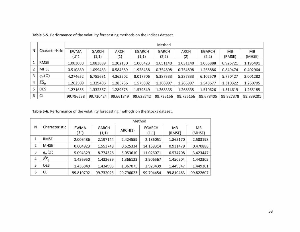
53
Table 5‐5. Performance of the volatility forecasting methods on the Indices dataset.
N Characteristic Method
EWMA
GARCH (1,1)
ARCH (1)
EGARCH (1,1)
GARCH (2,2)
ARCH (2)
EGARCH (2,2)
MB (RMSE)
MB (MHSE)
1 RMSE 1.003088 1.083889 1.202130 1.066423 1.051140 1.051140 1.056888 0.926721 1.195491 2 MHSE 0.510880 1.099483 0.584689 1.928458 0.754898 0.754898 1.268886 0.849474 0.402964 3 4.274652 6.785631 4.363502 8.017706 5.387333 5.387333 6.102579 5.770427 3.001282 4 1.262509 1.329406 1.285756 1.575892 1.266997 1.266997 1.548677 1.310322 1.260705 5 OES 1.271655 1.332367 1.289575 1.579549 1.268335 1.268335 1.510626 1.314619 1.265185 6 CL 99.796638 99.730424 99.661849 99.628742 99.735156 99.735156 99.678405 99.827378 99.839201
Table 5‐6. Performance of the volatility forecasting methods on the Stocks dataset.
N Characteristic Method
EWMA
GARCH (1,1)
ARCH(1) EGARCH (1,1)
MB (RMSE)
MB (MHSE)
1 RMSE 2.006486 2.197144 2.424559 2.186051 1.865170 2.5831982 MHSE 0.604923 1.553748 0.625334 14.168314 0.931479 0.4708883 5.094329 8.774326 5.053610 11.026071 6.574708 3.4234474 1.436950 1.432639 1.366123 2.906567 1.450504 1.4423055 OES 1.436849 1.434995 1.367075 2.923439 1.449347 1.4493016 CL 99.810792 99.732023 99.796023 99.704454 99.810463 99.822607

54
Table 5‐7. Performance of the volatility models and implied volatility for the Indices data subset.
N Characteristic
Method
EWMA
GARCH (1,1)
ARCH (1)
EGARCH (1,1)
GARCH (2,2)
ARCH (2)
EGARCH (2,2)
MB (RMSE)
MB (MHSE)
IV1
1 RMSE 1.090791 1.171080 1.388507 1.138602 1.137115 1.137115 1.127102 0.991736 1.286520 1.062791 2 MHSE 0.546538 1.013394 0.600877 1.791266 0.727686 0.727686 1.033894 1.062797 0.420414 0.511294 3 4.624267 7.299857 4.982415 9.831520 5.750332 5.750332 7.443971 7.290430 3.038510 4.257364 4 1.222764 1.133752 1.191009 1.561176 1.130966 1.130966 1.280882 1.560017 1.167447 1.189892 5 OES 0.468067 0.907141 0.702527 1.544002 0.674703 0.674703 0.772661 0.477010 0.467509 0.952244 6 CL 99.8344 99.7681 99.8012 99.7350 99.7847 99.7847 99.8012 99.8675 99.8675 99.7846
Table 5‐8. Performance of the volatility models and implied volatility for the Stocks data subset.
N Characteristic
Method
EWMA
GARCH (1,1)
ARCH (1)
EGARCH (1,1)
GARCH (2,2)
ARCH (2)
EGARCH (2,2)
MB (RMSE)
MB (MHSE)
IV2
1 RMSE 3.636001 3.642840 4.035042 3.408410 3.649005 3.649005 3.445134 3.237717 5.684578 3.201078 2 MHSE 1.296614 1.726116 0.881681 2.474553 1.530718 1.530718 1.608248 1.908309 0.806629 1.223559 3 5.808708 7.311894 5.489278 8.973477 6.704227 6.704227 6.956462 7.383313 2.833592 5.918723 4 2.616192 1.905565 1.690664 2.016285 2.101178 2.101178 1.883677 2.338671 1.934981 2.181829 5 OES 1.540882 1.161122 1.360862 1.075147 0.973995 0.973995 1.134165 1.179503 1.857380 1.294764 6 CL 99.8438 99.7321 99.7098 99.7098 99.7545 99.7545 99.6875 99.8438 99.7321 99.7545
1 Implied volatility is not included in Model Blending procedures.

55
5.5 Results of implied volatility surface modeling In this appendix we present the results of the modeling volatility skews for each of the
underlying assets. The errors for different types of tests and underlying are presented in Tables 5‐9 –
5‐17.
Table 5‐9. Performance of different volatility surface models on options of the AEX index.
N Model Quality of
fit
Static models Dynamic models 1 day
forecast 5 days forecast
1 day forecast
5 days forecast
1 Cubic 1.28626 3.21429 6.37292 3.99260 13.4539 2 Spline 1.05448 2.61850 5.39306 3.78533 9.41520 3 SABR 3.88212 5.62535 8.00410 5.62627 8.37488 4 PSABR 1.64033 3.48644 6.29141 6.05896 8.83062 5 Sticky Strike N/A 1.97364 4.36168 N/A N/A
Table 5‐10. Performance of different volatility surface models on options of the German stock index DAX.
N Model Quality of
fit
Static models Dynamic models 1 day
forecast 5 days forecast
1 day forecast
5 days forecast
1 Cubic 1.34813 3.25822 5.99786 3.48532 7.19360 2 Spline 0.84351 1.96317 4.06831 2.01622 4.57051 3 SABR 4.00186 5.08159 6.37802 5.08352 6.70261 4 PSABR 1.89345 2.83703 4.86227 4.74022 6.49834 5 Sticky Strike N/A 1.21387 2.95181 N/A N/A
Table 5‐11. Performance of different volatility surface models on options of the European stock index EURSTOXX.
N Model Quality of
fit
Static models Dynamic models 1 day
forecast 5 days forecast
1 day forecast
5 days forecast
1 Cubic 0.33500 1.65018 4.55425 1.82739 5.44496 2 Spline 0.31123 1.66325 4.56096 2.16492 5.96404 3 SABR 4.76126 5.18839 8.44978 5.19007 7.33259 4 PSABR 2.89203 3.40392 6.20050 3.64290 5.71112 5 Sticky Strike N/A 0.87453 2.38508 N/A N/A

56
Table 5‐12. Performance of different volatility surface models on options of the FTSE 100 – the UK equity index.
N Model Quality of
fit
Static models Dynamic models 1 day
forecast 5 days forecast
1 day forecast
5 days forecast
1 Cubic 0.33445 1.65999 4.58970 1.84163 5.50039 2 Spline 0.31083 1.67336 4.59633 2.17110 5.94110 3 SABR 4.26895 4.56957 8.48371 4.57191 6.89312 4 PSABR 2.86000 3.39127 6.17133 3.58511 5.79384 5 Sticky Strike N/A 0.87875 2.39056 N/A N/A
Table 5‐13. Performance of different volatility surface models on options of the XJO index – the Australian equity index.
XJO
N Model Quality of
fit
Static models Dynamic models 1 day
forecast 5 days forecast
1 day forecast
5 days forecast
1 Cubic 2.97195 11.01804 11.60088 9.99524 12.51182 2 Spline 2.87676 9.92295 10.63055 7.91253 8.84867 3 SABR 9.13593 13.43551 14.81607 13.42370 14.45272 4 PSABR 4.13998 9.56873 11.04536 11.20640 12.45780 5 Sticky Strike N/A 6.45673 7.91869 N/A N/A
Table 5‐14. Performance of different volatility surface models on implied volatility of the Deutsche Bank shares.
DBK
N Model Quality of
fit
Static models Dynamic models 1 day
forecast 5 days forecast
1 day forecast
5 days forecast
1 Cubic 7.74958 17.13035 36.88834 50.52760 136.69437 2 Spline 6.96815 14.86619 33.51260 28.45704 76.44249 3 SABR 16.68262 26.54118 55.61741 26.56520 46.13593 4 PSABR 8.78661 17.59187 35.20103 21.83207 35.48460 5 Sticky Strike N/A 13.59281 27.14709 N/A N/A
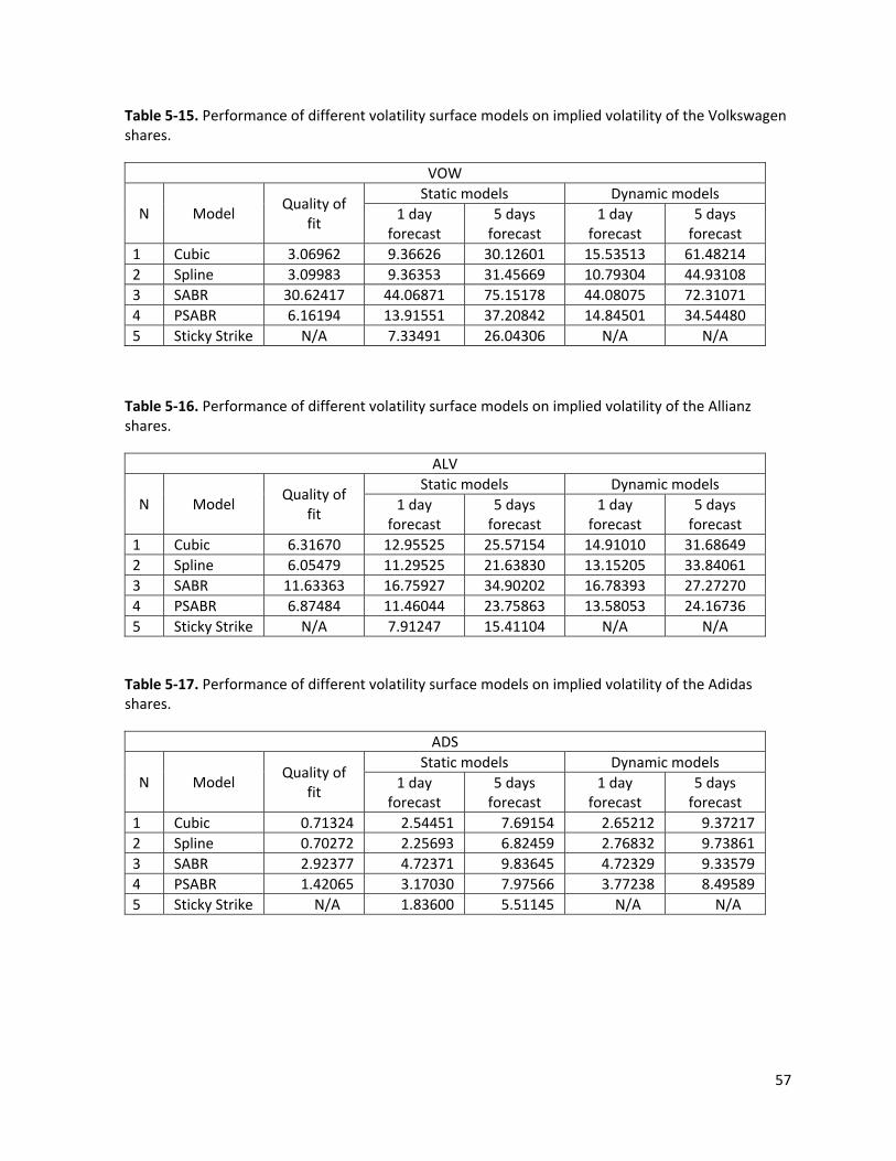
57
Table 5‐15. Performance of different volatility surface models on implied volatility of the Volkswagen shares.
VOW
N Model Quality of
fit
Static models Dynamic models 1 day
forecast 5 days forecast
1 day forecast
5 days forecast
1 Cubic 3.06962 9.36626 30.12601 15.53513 61.48214 2 Spline 3.09983 9.36353 31.45669 10.79304 44.93108 3 SABR 30.62417 44.06871 75.15178 44.08075 72.31071 4 PSABR 6.16194 13.91551 37.20842 14.84501 34.54480 5 Sticky Strike N/A 7.33491 26.04306 N/A N/A
Table 5‐16. Performance of different volatility surface models on implied volatility of the Allianz shares.
ALV
N Model Quality of
fit
Static models Dynamic models 1 day
forecast 5 days forecast
1 day forecast
5 days forecast
1 Cubic 6.31670 12.95525 25.57154 14.91010 31.68649 2 Spline 6.05479 11.29525 21.63830 13.15205 33.84061 3 SABR 11.63363 16.75927 34.90202 16.78393 27.27270 4 PSABR 6.87484 11.46044 23.75863 13.58053 24.16736 5 Sticky Strike N/A 7.91247 15.41104 N/A N/A
Table 5‐17. Performance of different volatility surface models on implied volatility of the Adidas shares.
ADS
N Model Quality of
fit
Static models Dynamic models 1 day
forecast 5 days forecast
1 day forecast
5 days forecast
1 Cubic 0.71324 2.54451 7.69154 2.65212 9.37217 2 Spline 0.70272 2.25693 6.82459 2.76832 9.73861 3 SABR 2.92377 4.72371 9.83645 4.72329 9.33579 4 PSABR 1.42065 3.17030 7.97566 3.77238 8.49589 5 Sticky Strike N/A 1.83600 5.51145 N/A N/A

58
6 Bibliography Black, F., & Scholes, M. (1973). The Pricing of Options and Corporate Liabilities. Journal of Political
Economy , 637–654.
Engle, R. (1982). Autoregressive conditional heteroscedasticity with estimates of the variance of
United Kingdom inflation. Econometrica , 987–1007.
Hafner, R., & Wallmeier, M. (2000). The Dynamics of DAX Implied Volatilities.
Hagan, P., Kumar, D., Lesniewski, A., & Woodward, D. (2002). Managing Smile Risk. Wilmott
Magazine , 84‐108.
Hastie, T., Tibshirani, R., & Friedman, J. (2002). The Elements of Statistical Learning. Springer
Series in Statistics.
Hull, J. C. (2002). Options, futures and other derivatives. New Jersey: Prentice Hall.
J. Knight, S. S. (2007). Forecasting volatility in the financial markets. London: Elsevier.
J.P. Morgan/Reuters. (1996). RiskMetrics ‐ Technical Document. New York: J.P. Morgan/Reuters.
McNeil, A. (1999). Extreme Value Theory for Risk Managers.
McNeil, F. &. (2005). Quantitative Risk Management: Concepts, Techniques, and Tools. Princeton
University Press.
Nelson, D. (1991). Conditional Heteroskedasticity in Asset Returns: A New Approach.
Econometrica , 347–370.
Poon, S. H. (2005). A practical guide to forecasting financial market volatility. Chichester: John
Wiley and Sons, ltd.
Poon, S. (2008). SABR.
Shlens, J. (2005). A Tutorial on Principal Component Analysis.
59
Tsai, H. (2006). A Note on Inequality Constraints in the GARCH model. Iowa: The University of
Iowa.
Tsay, R. S. (2005). Analysis of Financial Time Series. Wiley‐Interscience; 2nd edition .
West, G. (2005). Calibration of the SABR Model in Illiquid Markets. Applied Mathematical Finance
, 371‐385.
Wilmott, P., Howison, S., & Dewynne, J. (1995). The Mathematics of Financial Derivatives.
Cambridge: Cambridge University Press.
Witten, H. (2005). Data Mining: practical machine learning tools and techniques. Elsevier.