1

Volatility Regimes and Cross-market Correlation Dynamics in theDetermination of the Optimal International Equity Portfolio

Ming-Yuan Leon LiAssociate Professor

Department of Accountancy and Graduate Institute of Finance and BankingNational Cheng Kung University, TaiwanNo.1, Ta-Hsueh Road, Tainan 701, Taiwan

TEL: 886-6-2757575 Ext. 53421, FAX: 886-2744104E-mail: lmyleon@mail.ncku.edu.tw

2

Volatility Regimes and Cross-market Correlation Dynamics in theDetermination of the Optimal International Equity Portfolio

ABSTRACTA Markov-switching technique is used to examine co-movement dynamics between domestic and global

stock markets and to develop a state-varying approach to the design of an international portfolio. A

bivariate Markov switching ARCH (SWARCH) model is designed to evaluate four possible

combinations of the volatility states which can characterize both the domestic and world markets, thus

allowing the generation of state-varying portfolio loadings on the basis of 4-state correlations. The

following conclusions are drawn. First, the domestic and global markets are more strongly correlated

when both simultaneously find themselves in the same state of volatility. Conversely, this correlation is

weaker when a different volatility state characterizes each market. Furthermore, the circumstances in

which both the domestic and global stock markets simultaneously experience high levels of volatility

prove strongest cross-market correlations, and result in least effective at reducing the risk stemming

from international portfolio diversification. Next, this study determines state-varying portfolio loadings

which prove effective at the task of asset allocation, particularly under conditions of market volatility.

Finally, filtering structural changes out from the variance-switching process leads to a considerable

decrease of the time variation involved in generating state-varying portfolio loadings, which, in turn,

leads to lower transaction costs when compared to the performance of the conventional GARCH

model.

JEL classification: G11, G15

Keywords: International diversification; volatility; cross-market correlation;Markov-switching model; GARCH

3

I. Introduction

A state-varying approach forms the backbone of this analysis of the dynamics

underlying interactions among global stock markets. The purpose of the study is to

determine the optimal allocation of international equity to a portfolio consisting of

differentially weighted stock assets on the basis of their state-varying characteristics.

More specifically, four configurations of the volatility states of domestic and world

market returns are determined by the bivariate Markov-switching ARCH (hereafter,

SWARCH) model established by this study. Portfolio loading under state-varying

conditions can then be determined on the basis of the measures of the correlations

among the four states. Data from the stock markets of G7 countries are employed to

demonstrate the feasibility of the proposed model. Finally, a comparative analysis is

performed between portfolio weights calculated using either the bivariate SWARCH

or the bivariate GARCH model, in order to identify differences between state-varying

and time-varying characteristics.1

The benefits of investing in international equity are widely recognized,

especially with regards to increased efficiency and decreased risk. Research into the

international diversification of investment portfolios often emphasizes that the

potential of such behavior for bringing about a reduction of systematic risk below the

1 Modeling of the volatility of stock returns is commonly done using an ARCH (auto-regressiveconditional heteroskedasticity) model originally proposed by Engle (1982) and subsequently extendedby Bollerslev’s (1986) GARCH (generalized ARCH) model.

4

level incurred by investing in domestic securities alone results from structural and

cyclical differences among various economies.2 While risk reduction is a well-known

phenomenon in this context, its extent may be attenuated by the strength of the

correlation existing between domestic and global markets. In fact, such a cross-market

correlation and the potential for risk reduction are negatively correlated; that is, the

more strongly are correlated different markets, the smaller is the potential reduction in

risk. In terms of portfolio diversification, an additional difficulty is ascertaining the

optimal weights to be given to the different stock assets under consideration. Market

correlation strength also exerts a considerable influence on the determination of such

portfolio loadings. Consequently, this study considers the accurate measurement of

the strength of the correlation between domestic and international markets to be a key

issue in international stock allocation.

A number of studies have contributed to the literature on the diversification of

international investments. For example, Byers and Peel (1993) examine stock market

interdependence and returns on investment resulting from international diversification

on the basis of data from the national stock markets of Japan, the Netherlands, the

U.K., the U.S., and West Germany. Chang (2001) provides evidence that there exist

2 International diversification offers benefits which stem from different circumstances. For example,individual national stock markets vary considerably in terms of returns and risks, a fact which becomesclear when one considers the persistence of barriers to international diversification, such as marketsegmentation, insufficient liquidity, exchange rate controls, and inaccessibility of information. As aresult of such circumstances, cross-market correlations have been relatively weak.

5

long-run benefits for investors in Taiwan who include in their portfolios shareholdings

from the equity markets of the country’s major trading partners, including Hong Kong,

Japan, South Korea, Thailand, and the U.S. Investing heavily in an emerging market

such as Thailand seems to imply increased risk, a concern that is addressed by Fifield

et al. (2002) in their discussion of the costs and benefits of investing in emerging

stock market equities.

Market integration has been another focal point of the research, some of which

investigates the effects of recent developments in Europe. Kempa and Nelles (2001),

for instance, analyze international correlations and excess returns in European stock

markets both before and after the EMU’s coming into effect. The countries of the

industrialized world in general are frequently targeted by such research. Tahai et al.

(2004) employ a vector error correction model to investigate financial co-integration

among G7 equity markets. Heimonen (2002) evaluates stock market integration

between Finland, Germany, Japan, the U.K., and the U.S., from the point of view of

the international investor.

Finally, the phenomenon of market co-movements has also been analyzed, in

particular by Syriopoulos (2004), who shows that long-run co-movements exist

among various Central European stock markets. It is suggested that such behavior

implies that the potential to diversify risk and attain superior portfolio returns by

6

investing in different Central European markets may be limited for international

investors.

As opposed to these several studies, this paper emphasizes that international

stock markets are much more closely correlated when markets are struggling through

a period of crisis. Along similar lines of reasoning, country portfolio returns have

been shown to correlate much more strongly during turbulent times in securities

markets (e.g., King and Wadhwani, 1990; Erb et al. 1994; Lin et al. 1994; Longin and

Solnik, 1995; Karolyi and Stulz, 1996; Boyer et al. 1999; Longin and Solnik, 2001;

Jacquier and Marcus, 2001; Ang and Bekaert, 2002; Forbes and Rigobon, 2002; Bae

et al. 2003 and Das and Uppal, 2004). Another case in point is the fact that declines

of most major stock indices occurred concurrently during the crash of October 1987

(Roll, 1988). At such times of chaos and instability, the need is more acutely felt for

the benefits derived from diversification-related risk reduction. However, as

previously noted, the stronger correlations observed among markets suggest that these

benefits are largely lost at such times.

Upon closer scrutiny of studies such as these, it is possible to discern a common,

time-based factor from which stem global stock price fluctuations. For instance,

Longin and Solnik (1995) identify an intensification of cross-market correlations at

times of crisis when markets are highly volatile. This implies that inevitable changes

7

in volatility over the long run adversely impact the advantages of international

diversification. This contention is supported by a study of the linkages between the

U.S. and Latin American stock markets, which was conducted using co-integration

models highlighting structural shifts in long-run dynamics (Fernandez-Serrano and

Sosvilla-Rivero, 2003). The primary conclusion drawn from this analysis is that gains

derived from international diversification are limited in the case of long-term

investments.

This study attempts to extend existing research and to improve on some of its

perceived shortcomings. On the one hand, many studies consider time to be the

primary explanatory variable in the analysis of non-constant correlations;

consequently, researchers proceed either by dividing the entire sampling period into

several sub-periods or by employing a time-varying approach. In contrast to such an

approach, a state-varying framework here forms the basis of our investigation of

cross-market correlation dynamics.

On the other hand, it is generally accepted that market volatility is a crucial

element of the study of stock market behavior. In times of crises, financial or political

upheavals are associated with increased market volatility, as revealed by the

examination of realized stock returns. In terms of the overseas extension of portfolio

diversification, distinct high/low volatility (HV/LV) regimes have been shown to exist

8

in international stock markets (Hamilton and Susmel, 1994; Ramchand and Susmel,

1998; and Li and Lin, 2003). Unfortunately, the accurate characterization of various

volatility regimes is impossible in the context of frequently encountered research

based on simplified settings with constant parameters.

Based on such observations, therefore, we develop the bivariate SWARCH

model to determine whether a HV/LV regime exists at certain dates, and to measure

the size of the co-movements occurring among domestic and world markets in various

states of volatility. The model also serves the purpose of devising a strategy for the

development of a state-varying international portfolio.

Investigating much the same relationships as those under scrutiny in the present

study, such as Ramchand and Susmel (1998) observed that the correlation between the

U.S. domestic stock market and other national markets was strongest when the former

was experiencing high volatility; Ang and Bekaert (2002) used a regime switching

model to analyze the effect of time-varying correlation on the benefit of international

diversification and demonstrated that the existence of high correlation and high

volatility bear market regime does not negate the benefits of international

diversification; Das and Uppal (2004) characterized the returns on international equity

market by jumps occurring at the same time and studied the effect of the systematic

risk induced by the jumps. They found that while systematic risk affects the allocation

9

of wealth between the riskless and risky assets, it has a small effect on the

composition of the portfolio of only-risky assets, and reduces marginally the gains to

a US investor from international diversification.

While based on a similar framework consisting of state variables, the analysis

presented in this study differs from theirs as follows. First, this study adopts the

CAPM perspective to investigate two independent components of the risks at play in

international diversification: (1) the world market risk factor (systematic risk), and (2)

the domestic market risk factor (nonsystematic risk). This bifurcation leads to a

further distinction with the study of Ramchand and Susmel. Whereas they utilized a

dual-state specification (HV/LV states) in their analysis of cross-market correlations,

we consider both the market-wide (systematic risk) and the idiosyncratic

(nonsystematic risk) components to be subject to distinct volatility state switching

processes. Therefore, different combinations of volatility states are analyzed on the

basis of four-way correlations among domestic and world markets.

In sum, a novel approach is presented to research into issues related to volatility

regimes and market correlations with the aim of designing a strategy enabling the

development of a dynamic investment portfolio. Its novelty results from the fact that

the determination of the optimal allocation ratio of stock assets relies heavily on being

able to accurately measure domestic-global market correlations, an aspect addressed

10

in this study.

Finally, the following are examples of issues addressed in this study:

- Is the magnitude of market correlations consistent across various combinations

of volatility regimes? If no such consistency exists, what are the relationships among

various market volatility regimes and correlations?

- If cross-market correlations are state dependent, can a state-varying framework

help investors design a more effective strategy for investing in international stock?

- Is the state-varying framework more or less valid under conditions of highly

variable states?

- Is the loading of a portfolio based on state-varying considerations associated

with the higher magnitude of variations in time?

- Are the benefits of the reduction in risk stemming from the international

diversification of an investment portfolio consistent among various market volatility

states? If not, what are the relationships among such benefits and market volatility

states?

To our knowledge, few studies have addressed such significant issues regarding

the determination of international equity asset allocation.

The remainder of this paper is organized as follows. Section 2 outlines the

models used in this study: (1) a conventional bivariate GARCH model for the

11

development of a time-varying framework, and (2) a bivariate SWARCH model in the

context of the state-varying approach. Subsequently, Section 3 presents the empirical

results and provides economic and financial explanations. Finally, Section 4 draws

conclusions.

12

2. Model Specifications

2.1 Bivariate GARCH Model: Optimal Asset Allocation via a Time-Varying

System

Tools facilitating the design of effective strategies for the dynamic allocation of

stock assets have long been sought, a fact attested to by the considerable interest

generated by recent relevant research. In the existing research, it is invariably the case

that frameworks are elaborated to enable the determination of dynamic portfolio

loadings, the estimation of which is based on time-varying variance-covariance matrix

derived from ARCH or GARCH models. Furthermore, in academic circles, it is

generally acknowledged that correlations among domestic and global market returns,

along with corresponding return variances, are the key factors in building the optimal

international equity portfolio. Consequently, the possibility of designing a more

effective portfolio of international stock assets based on consideration of the dynamic

relationships existing between volatility regimes and cross-market correlations is

investigated herein by the bivariate GARCH model relying on time-varying

characteristics as a benchmark. The following is an outline of the specifications of the

model and its potential limitations.

Given that rty and rt

x stand for the return rates in global and domestic stock

markets, respectively, the bivariate GARCH model used in this study can be specified

13

as follows. First:

yt

pi

i

yit

yi

yyt err

10 (1)

xt

pi

i

xit

xi

xxt err

10 (2)

where ety and et

x are residuals at time t. These residuals are depicted by the following

equation:

),0(~|| 11 ttxt

yt

tt HBNee

e

(3)

where Ψt-1 refers to the information available at time t-1; BN denotes the bivariate

normal distribution; and Ht is a time-varying 2x2 positive definite conditional

variance-covariance matrix. This matrix is depicted as:

xt

xyt

xyt

yt

t hhhh

H,

,

(4)

and its specific elements are specified using the following equations:

14

m

l

ylt

ylt

yjt

q

j

yjt

yyt heh

1

2

10 )( (5)

m

l

xlt

xlt

xjt

q

j

xjt

xxt heh

1

2

10 )( (6)

2/1, )( xt

yt

xyt hhh (7)

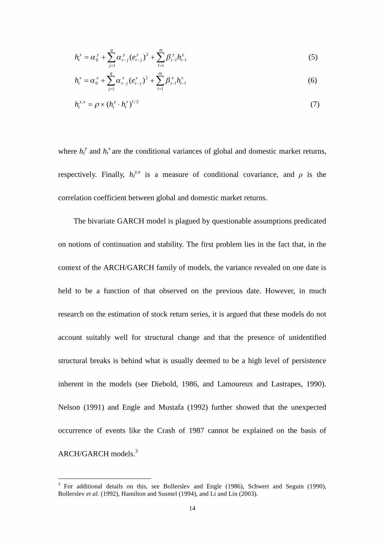
where hty and ht

x are the conditional variances of global and domestic market returns,

respectively. Finally, hty,x is a measure of conditional covariance, and ρis the

correlation coefficient between global and domestic market returns.

The bivariate GARCH model is plagued by questionable assumptions predicated

on notions of continuation and stability. The first problem lies in the fact that, in the

context of the ARCH/GARCH family of models, the variance revealed on one date is

held to be a function of that observed on the previous date. However, in much

research on the estimation of stock return series, it is argued that these models do not

account suitably well for structural change and that the presence of unidentified

structural breaks is behind what is usually deemed to be a high level of persistence

inherent in the models (see Diebold, 1986, and Lamoureux and Lastrapes, 1990).

Nelson (1991) and Engle and Mustafa (1992) further showed that the unexpected

occurrence of events like the Crash of 1987 cannot be explained on the basis of

ARCH/GARCH models.3

3 For additional details on this, see Bollerslev and Engle (1986), Schwert and Seguin (1990),Bollerslev et al. (1992), Hamilton and Susmel (1994), and Li and Lin (2003).

15

Another difficulty with the GARCH model is its assumption of the stability of

domestic-global market return correlations. In terms of the conventional modeling

framework, the variances (hty and ht

x) and covariance (hty,x) are considered to be

time-varying, whereas the correlation coefficient (the ρ parameter) is treated as a

constant, as designed in Bollerslev (1990), Baillie and Bollerslev (1990), and Chan et

al. (1991), among many others. However, developing an international portfolio relies

heavily on the accurate measurement of these variances and correlations, both of

which, in reality, may vary. Moreover, the weight attributed to each domestic/global

asset in a given portfolio is a function of these key parameters combined.

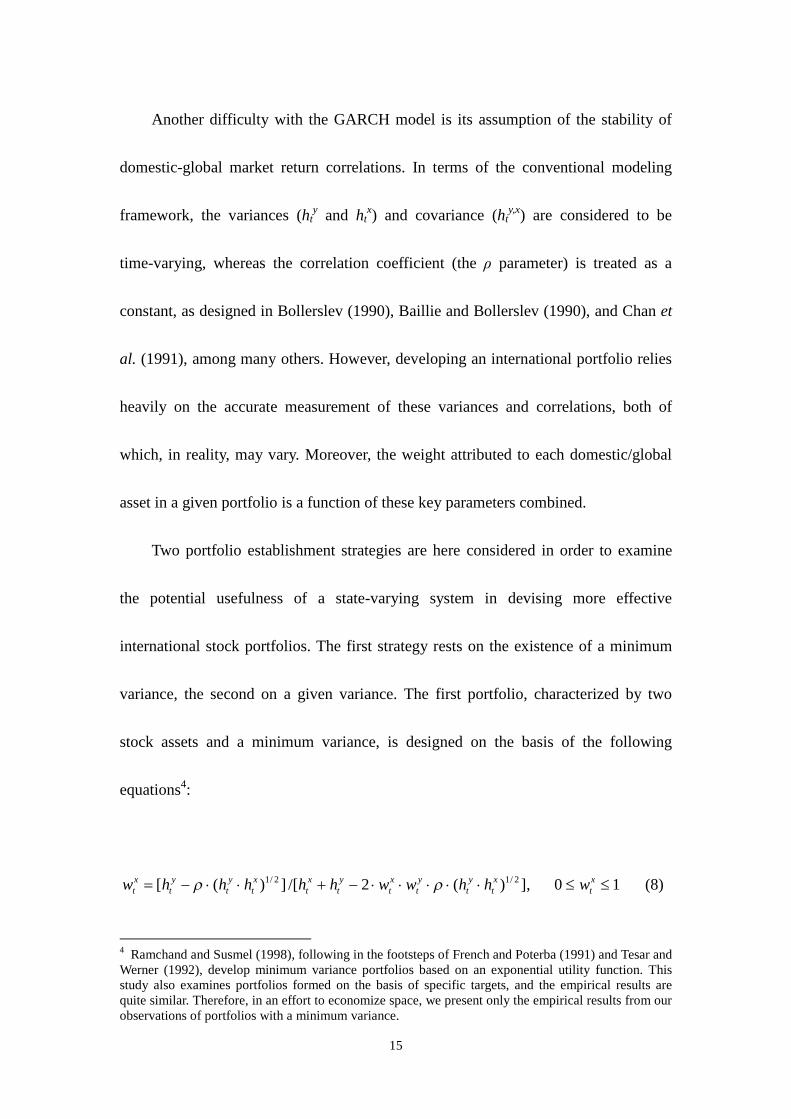
Two portfolio establishment strategies are here considered in order to examine

the potential usefulness of a state-varying system in devising more effective

international stock portfolios. The first strategy rests on the existence of a minimum

variance, the second on a given variance. The first portfolio, characterized by two

stock assets and a minimum variance, is designed on the basis of the following

equations4:

10],)(2/[])([ 2/12/1 xt

xt

yt

yt

xt

yt

xt

xt

yt

yt

xt whhwwhhhhhw (8)

4 Ramchand and Susmel (1998), following in the footsteps of French and Poterba (1991) and Tesar andWerner (1992), develop minimum variance portfolios based on an exponential utility function. Thisstudy also examines portfolios formed on the basis of specific targets, and the empirical results arequite similar. Therefore, in an effort to economize space, we present only the empirical results from ourobservations of portfolios with a minimum variance.

16

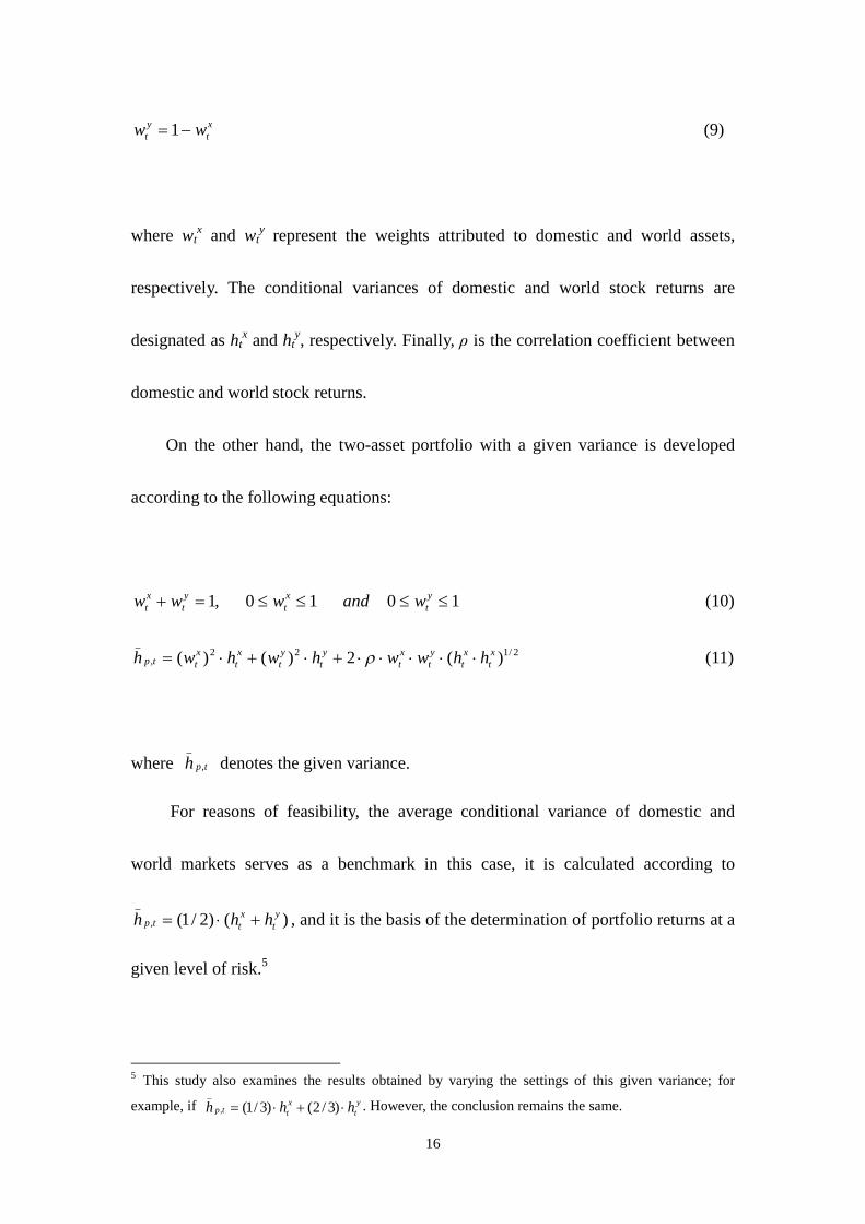
xt

yt ww 1 (9)

where wtx and wt

y represent the weights attributed to domestic and world assets,

respectively. The conditional variances of domestic and world stock returns are

designated as htx and ht

y, respectively. Finally,ρis the correlation coefficient between

domestic and world stock returns.

On the other hand, the two-asset portfolio with a given variance is developed

according to the following equations:

1010,1 yt

xt

yt

xt wandwww (10)

2/122,

_

)(2)()( xt

xt

yt

xt

yt

yt

xt

xttp hhwwhwhwh (11)

where tph ,

_

denotes the given variance.

For reasons of feasibility, the average conditional variance of domestic and

world markets serves as a benchmark in this case, it is calculated according to

)()2/1(,

_y

txttp hhh , and it is the basis of the determination of portfolio returns at a

given level of risk.5

5 This study also examines the results obtained by varying the settings of this given variance; for

example, if yt

xttp hhh )3/2()3/1(,

_. However, the conclusion remains the same.

17

2.2 Bivariate SWARCH Model: Optimal Asset Allocation via a State-Varying

System

The volatility of stock returns have been shown to be substantially higher than

average at certain times on the basis of the careful examination of the rates of realized

stock returns. Furthermore, a highly persistent volatility is associated with lower

predictive accuracy in many studies employing GARCH models. For instance, two

influential such studies attribute the high level of persistence in GARCH models to

structural changes emerging in the process of estimating stock return volatility

(Diebold, 1986; Lamoureux and Lastrapes, 1990).

The partitioning of the period covered by the sample into distinct phases on the

basis of dummy variables allows not only the control of volatility levels but also the

conceptualization of these structural changes. However, defining such dummy

variables rests on the subjective selection of cutoff dates. The resultant arbitrariness

prevents the accurate prediction of the timing of the structural changes.

This study contends that a model making it possible to identify the timing of

structural changes on the basis of the available data alone would better account for the

behavior of stock returns. To this end, a bivariate volatility-switching model is

developed in order to accurately identify discrete jumps in stock return volatility.

Such a model identifies the HV/LV regimes of domestic and global market returns at

18

each distinct point in time. A state-varying framework is then developed for devising

asset allocation strategies.

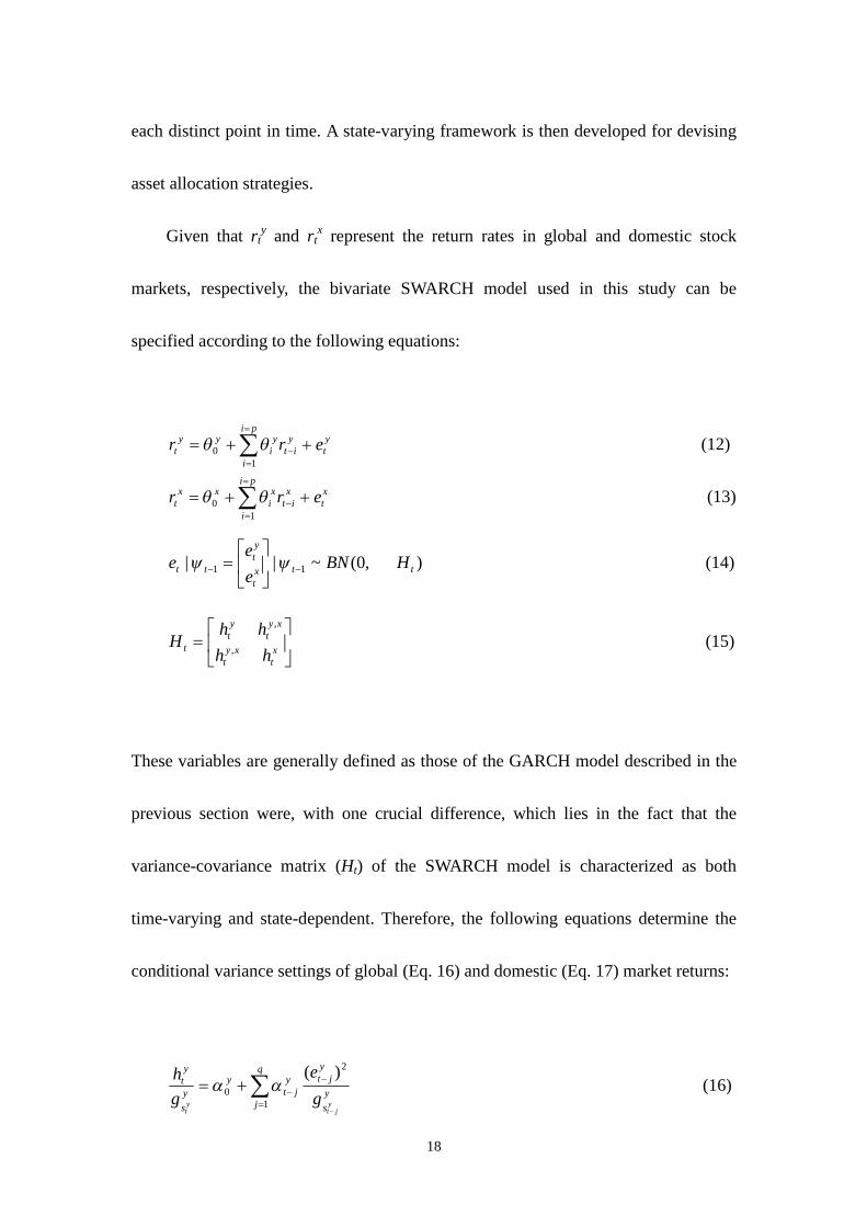
Given that rty and rt

x represent the return rates in global and domestic stock

markets, respectively, the bivariate SWARCH model used in this study can be

specified according to the following equations:

yt

pi

i

yit

yi

yyt err

10 (12)

xt

pi

i

xit

xi

xxt err

10 (13)

),0(~|| 11 ttxt

yt

tt HBNee

e

(14)

xt

xyt

xyt

yt

t hhhh

H,

,

(15)

These variables are generally defined as those of the GARCH model described in the

previous section were, with one crucial difference, which lies in the fact that the

variance-covariance matrix (Ht) of the SWARCH model is characterized as both

time-varying and state-dependent. Therefore, the following equations determine the

conditional variance settings of global (Eq. 16) and domestic (Eq. 17) market returns:

ys

yjt

q

j

yjt

yys

yt

yjt

yt

g

e

gh

2

10

)( (16)

19

xs

xjt

q

j

xjt

xxs

xt

xjt

xt

g

e

gh

2

10

)( (17)

where sty and st

x are unobservable state variables, for which the possible values are 1,

2, 3,… n, and which are employed to indicate the volatility regime at time t

characterizing global and domestic market returns, respectively.

This model, thus developed on the basis of two dimensions, is intended as an

extension of Hamilton and Susmel’s (1994) one-dimensional SWARCH model. It

should be noted, however, that the bivariate framework used herein involves

extremely intensive computations. Therefore, in an effort to keep time requirements

within reasonable bounds, two volatility regimes only are examined: The HV and LV

states for both global market returns (sty =｛1, 2｝) and domestic market returns (st

x=

｛1, 2｝).

Certain manipulations are required while developing such a model. For instance,

without reducing generalization, g1y and g1

x, the scale coefficients for regime I, are

normalized to unity; whereas g2y>1 and g2

x>1 in the case of regime II. More

specifically, the dynamics underlying the conditional variances involved in regime I

are accounted for by the conventional ARCH (q) process. On the other hand, the

conditional variances at play in regime II are defined as g2y and g2

x times those of

regime I in the equations for global and individual market returns, respectively. In the

20

special case in which g1y =g2

y=1 and g1x =g2

x=1, the two residual terms, eyt and ex

t,

remain consistent with the conventional ARCH (q) process.

Based on the assumption that two distinct volatility regimes characterize each

market return component, both global and domestic, covariance is modeled according

to the possible occurrence of four different volatility states. Such covariance can be

formulated as follows:

2/1,

, )( xt

ytss

xyt hhh x

tyt

(18)

Furthermore, the possibility of different combinations of volatility regimes

brings about a general system consisting of 4-state correlations: (1) ρ1,1, in which case

both global and individual market returns are in a state of low volatility (sty=1 and

stx=1; World=LV and Indl.=LV); (2)ρ2,1, where volatility is high in the case of global

market returns but low for individual market returns (sty=2 and st

x =1; World=HV and

Indl.=LV); (3) ρ1,2, where volatility is low in the case of global market returns and

high for individual market returns (sty=1 and st

x=2; World=LV and Indl.=HV); and (4)

ρ2,2, in which case both global and individual market returns are in a state of high

volatility (sty =2 and st

x =2; World=HV and Indl.=HV).

Based on this system thus described, the construction of the latent variable st on

21

the basis of the separate latent processes sty and st

x can be visually depicted as follows:

st=1: if sty=1 and st

x=1 -or- World=LV and Indl.=LV

st=2: if sty=2 and st

x=1 -or- World=HV and Indl.=LV

st=3: if sty=1 and st

x=2 -or- World=LV and Indl.=HV

st=4: if sty=2 and st

x=2 -or- World=HV and Indl.=HV

As was assumed in the case of the univariate analysis, st is an unobservable state

variable; however, in the present case, the state variable st is associated with possible

outcomes of 1, 2, 3 and 4. Furthermore, this state variable is held to follow a

first-order 4-state Markov chain model formulated as follows:

ijtt pisjsp )|( 1 (19)

The transition probability matrix of this model can be depicted as follows:

44342414

43332313

42322212

41312111

pppppppppppppppp

P (20)

22

The inclusion of multiple volatility states in the present model requires further

explanation. While it is true that, theoretically, the number of states under

consideration in a study such as this one can be extended to infinity, in actuality, their

number is limited. In the case of the present model, which is set to accommodate two

regimes only, a 2×2 transition probability matrix, with only 2 unknown probability

parameters, appears to be all that is required. However, the complexity inherent in

volatility switching models increases considerably when they are applied to the

estimation of multivariate systems. Consequently, accounting for the regime

switching process in the 4-state model employed in this study necessitates the

adoption of a 4×4 transition probability matrix and the estimation of 12 unknown

probability parameters.

Moreover, in this study, the world market index is considered to serve as a

synthetic holding of global assets, and the idiosyncratic risk pertaining to domestic

market assets is understood to decrease to an arbitrarily low level. In line with such

reasoning, variance of global and domestic market returns is here seen as being

subject to the distinct processes of the switching of volatility states characterizing

each of these types of market component. Thus, the volatility state variable for global

market returns (sty) is expected to be independent of that for individual market returns

(sτx) in the case of all t and τ. According to this hypothesis, the transition probability

23

matrix for the variable st of this 4-state model can be depicted as:

xyxyxyxy

xyxyxyxy

xyxyxyxy

xyxyxyxy

pppppppppppppppppppppppppppppppp

P

2222221212221212

2221221112211211

2122211211221112

2121211111211111

(21)

where ( yp11 , yp22 ) and ( xp11 , xp22 ) are the transition probabilities for sty and st

x,

respectively, and are derived on the basis of the following equations:

yyt

yt

yyt

yt pssppssp 221111 )2|2(,)1|1( (22)

xxt

xt

xxt

xt pssppssp 221111 )2|2(,)1|1( (23)

A comparison of the two ostensibly identical 4-state switching models depicted

in Eqs. 20 and 21 reveal significantly different in the numbers of population

parameters required to estimate. In the case of the general model presented in Eq. 20,

st follows a 4-state Markov chain, the transition matrix of which is restricted by the

condition that each column must sum to unity, hence the need for 12 probability

parameters. On the other hand, the estimation of only 4 (2+2) probability parameters

is required in the restricted 4-state model presented in Eq. 21.

Of course, the specifications underlying the elaboration of transition probability

24

matrix implied by Eq. 20 are very general in that they encompass various interactions

among the variance states of market returns at both the global and domestic levels

(see Hamilton and Lin, 1996). On the other hand, the necessity of accommodating a

very specific hypothesis about underlying variance states undeniably limits to a

considerable extent the generalizability of the preferred model presented in Eqs. 21-23.

Despite such limitations, the latter restricted model was decided upon in order to

ensure the manageability of the 4-state system studied herein and to facilitate the

convergence of the maximum likelihood procedure.6 This choice is further justified

by the very act of postulating the independence of the systematical and

non-systematical risk components examined in this study.

As has already been suggested, the bivariate SWARCH model developed in this

study bears a strong resemblance to those presented in previous studies (see

Ramchand and Susmel, 1998; Edwards and Susmel, 2003). However, whereas such

prior attempts rest on the assumption that the correlations examined are a function

only of the state of a single return series and employ a setting restricted to dual

correlations, we go one step further to define a setting of 4-state correlations.

With regard to the observed data, rt = (rty , rt

x) is taken to represent a 2×1 vector

6 This study has also developed a bivariate SWARCH model according to a 4X4 transition probabilitymatrix. Although such an unrestricted model is very general and encompasses different interactionsamong the variance states of both global and domestic market returns, it is intractable and its likelihoodfunction fails to converge in some cases. Moreover, some elements of the 4X4 switching probabilitymatrix considerably approach zero.

25

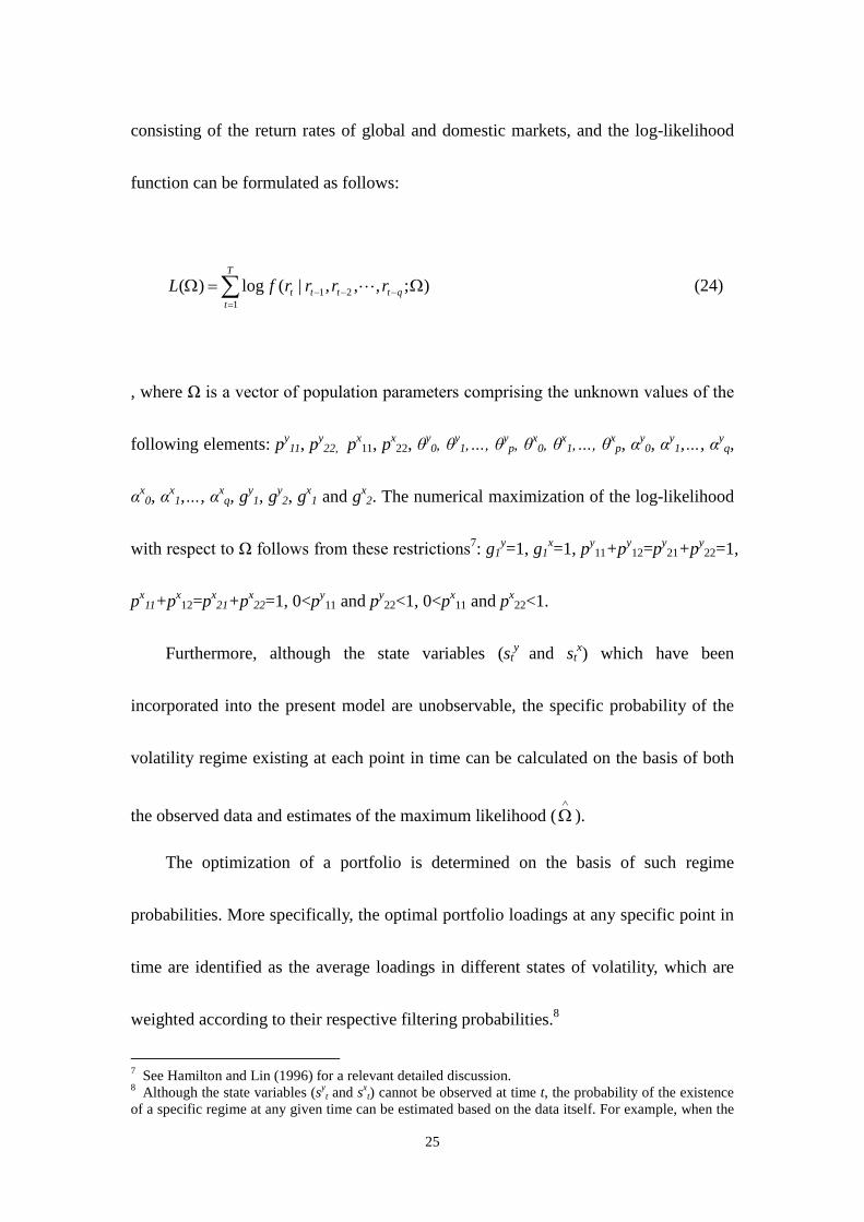
consisting of the return rates of global and domestic markets, and the log-likelihood

function can be formulated as follows:

T

tqtttt rrrrfL

121 );,,,|(log)( (24)

, whereΩ is a vector of population parameters comprising the unknown values of the

following elements: py11, py

22, px11, px

22,θy0, θy

1,…, θyp, θx

0, θx1,…, θx

p,αy0,αy

1,…,αyq,

αx0,αx

1,…,αxq, gy

1, gy2, gx

1 and gx2. The numerical maximization of the log-likelihood

withrespect to Ω follows from these restrictions7: g1y=1, g1

x=1, py11+py

12=py21+py

22=1,

px11+px

12=px21+px

22=1, 0<py11 and py

22<1, 0<px11 and px

22<1.

Furthermore, although the state variables (sty and st

x) which have been

incorporated into the present model are unobservable, the specific probability of the

volatility regime existing at each point in time can be calculated on the basis of both

the observed data and estimates of the maximum likelihood (

).

The optimization of a portfolio is determined on the basis of such regime

probabilities. More specifically, the optimal portfolio loadings at any specific point in

time are identified as the average loadings in different states of volatility, which are

weighted according to their respective filtering probabilities.8

7 See Hamilton and Lin (1996) for a relevant detailed discussion.8 Although the state variables (sy

t and sxt) cannot be observed at time t, the probability of the existence

of a specific regime at any given time can be estimated based on the data itself. For example, when the

26

As a final point on the design of the model used herein, it must be noted that the

discrete state variable is given two possible outcome values to reflect HV/LV regimes,

and the q-order obtained on the basis of prior-period error squares is used in

determining the conditional variance settings (see Eqs. 16 and 17). This implies that

the possible existence of 2(q+1) volatility states for every univariate stock return gained

on each date must be taken into account, which, in turn, suggests the need to consider

the possibility of facing (2q+1)2 variance-state combinations at each point in time in

the case of a bivariate SWARCH model. As a result, the value of q is set at 1 in the

following empirical analysis, thus bringing about the necessity of considering 16

possible variance-sate combinations on each date.

In sum, the bivariate SWARCH model defined in this section holds certain key

advantages over the conventional GARCH model presented earlier. First, discrete

adjustments made to the volatility switching system in the latter model resolve

difficulties stemming from the unrealistic assumption of the existence of a single,

constant correlation posited in the context of the former model. In other words, the

single measurement of correlation carried out with the GARCH model corresponds to

four such measurements in the case of the SWARCH model (compare Eqs. 7 and 18).

information set used to carry out this estimation includes signals dated up to time t, the regimeprobability is a filtering probability. It is also possible to use the information set encompassing theoverall sample period to provide an estimation at time t of the regime probability, which is then called asmoothing probability. Finally, a predicting probability refers to the regime probability based on an exante estimation, in which case the information set includes signals dated up to period t-1.

27

Second, the bivariate SWARCH model is set in such a way that the measurement

of variance is sensitive to changes according to both time and state. Specifically, the

variance dynamics at play in the context of an LV regime (regime I) are accounted for

by the conventional ARCH (q) process incorporated into the SWARCH model (see

Eqs. 16 and 17).

Finally, the use of a discrete jump process in the bivariate SWARCH model

allows the examination of structural changes occurring as a result of variations in

scale from gy1 (=1) to gy

2(>1) in the case of global market returns, and from gx1 (=1)

to gx2(>1) for domestic market returns. Thus being able to account for events

reflecting structural change effectively corrects the problem of a highly persistent

volatility which characterizes the conventional ARCH/GARCH models.

28

3. Empirical Results

3.1 Data

The overall data represent two levels of observation, the global and the national.

In the case of the latter category, the domestic market component of the model is

expressed in terms of the stock price indices of each individual G7 country, which

were collected from the Data Stream database. These indices, which account for a

minimum of 80% of the stock market capitalization of each country, are valued in U.S.

dollar. On the other hand, the following two indices are seen as proxies for assessing

the global market component of the model: (1) the world index, which is provided by

Morgan Stanley Capital International (MSCI hereafter), and (2) the equally weighted

world stock index (EWW hereafter), which averages various market indices by

attributing an equal weight to each one of them. The data thus collated was used to

create 14 (7X2) international portfolios which form the core of the analysis which

follows this section.

With regard to the specifics of the data, each entry corresponds to a recorded

observation, and each two consecutive such observations are separated by a week

(Wednesday to Wednesday). Collectively, these observations cover the period from

January 1980 to May 2007. The entire sample consists of 1,426 observations. The

descriptive statistics and correlation matrices performed on the data are presented in

29

Table 1.

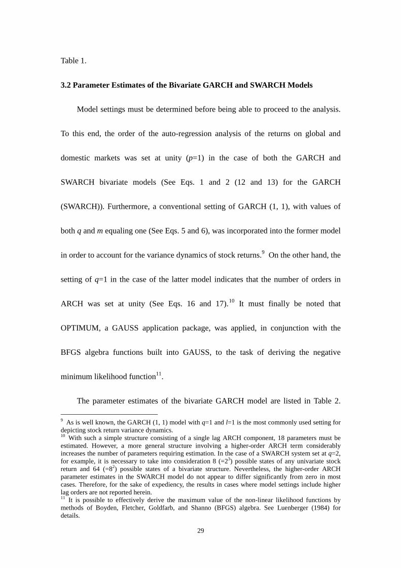
3.2 Parameter Estimates of the Bivariate GARCH and SWARCH Models

Model settings must be determined before being able to proceed to the analysis.

To this end, the order of the auto-regression analysis of the returns on global and

domestic markets was set at unity (p=1) in the case of both the GARCH and

SWARCH bivariate models (See Eqs. 1 and 2 (12 and 13) for the GARCH

(SWARCH)). Furthermore, a conventional setting of GARCH (1, 1), with values of

both q and m equaling one (See Eqs. 5 and 6), was incorporated into the former model

in order to account for the variance dynamics of stock returns.9 On the other hand, the

setting of q=1 in the case of the latter model indicates that the number of orders in

ARCH was set at unity (See Eqs. 16 and 17).10 It must finally be noted that

OPTIMUM, a GAUSS application package, was applied, in conjunction with the

BFGS algebra functions built into GAUSS, to the task of deriving the negative

minimum likelihood function11.

The parameter estimates of the bivariate GARCH model are listed in Table 2.

9 As is well known, the GARCH (1, 1) model with q=1 and l=1 is the most commonly used setting fordepicting stock return variance dynamics.10 With such a simple structure consisting of a single lag ARCH component, 18 parameters must beestimated. However, a more general structure involving a higher-order ARCH term considerablyincreases the number of parameters requiring estimation. In the case of a SWARCH system set at q=2,for example, it is necessary to take into consideration 8 (=23) possible states of any univariate stockreturn and 64 (=82) possible states of a bivariate structure. Nevertheless, the higher-order ARCHparameter estimates in the SWARCH model do not appear to differ significantly from zero in mostcases. Therefore, for the sake of expediency, the results in cases where model settings include higherlag orders are not reported herein.11 It is possible to effectively derive the maximum value of the non-linear likelihood functions bymethods of Boyden, Fletcher, Goldfarb, and Shanno (BFGS) algebra. See Luenberger (1984) fordetails.

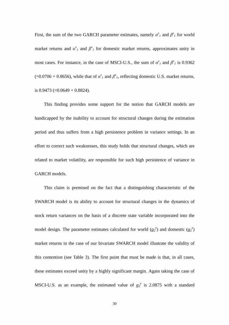
30

First, the sum of the two GARCH parameter estimates, namely αy1 and βy

1 for world

market returns and αx1 and βx

1 for domestic market returns, approximates unity in

most cases. For instance, in the case of MSCI-U.S., the sum of αy1 and βy

1 is 0.9362

(=0.0706 + 0.8656), while that ofαx1 andβx

1, reflecting domestic U.S. market returns,

is 0.9473 (=0.0649 + 0.8824).

This finding provides some support for the notion that GARCH models are

handicapped by the inability to account for structural changes during the estimation

period and thus suffers from a high persistence problem in variance settings. In an

effort to correct such weaknesses, this study holds that structural changes, which are

related to market volatility, are responsible for such high persistence of variance in

GARCH models.

This claim is premised on the fact that a distinguishing characteristic of the

SWARCH model is its ability to account for structural changes in the dynamics of

stock return variances on the basis of a discrete state variable incorporated into the

model design. The parameter estimates calculated for world (g2y) and domestic (g2

x)

market returns in the case of our bivariate SWARCH model illustrate the validity of

this contention (see Table 3). The first point that must be made is that, in all cases,

these estimates exceed unity by a highly significant margin. Again taking the case of

MSCI-U.S. as an example, the estimated value of g2y is 2.0875 with a standard

31

deviation of 0.1472, and the estimated value of g2x is 2.4436 with a standard deviation

of 0.1827. These estimates reflect differences in market volatility between regimes I

and II. Specifically, the level of volatility inherent in the world (domestic) market

returns of MSCI-U.S. under regime II is held to be 2.0875 (2.4436) times higher than

that of regime I.

Furthermore, the 99% confidence level of the estimations of g2y and g2

x do not

overlap with those of g1y and g1

x, that is, the values at unity. Consequently, in terms of

the SWARCH model designed in this study, sty=2 (the state variable for global

markets) and stx=2 (the state variable for domestic markets) are confidently held to

stand for the HV state, whereas sty=1 and st

x=1 represent the LV state.

This study further incorporates into its model a 4-state correlation system based

on the examination of various combinations of variance states. Corresponding

correlation estimates are shown to diverge significantly among various state

combinations in all cases. More specifically, with three exceptions only

(MSCI-Canada, EWW-Canada and EWW-Japan), rejection of the null hypothesis

postulating the existence of identical correlations is warranted on the basis of the LR

statistical analysis12 at a 1% level of significance13 (see the last row of Table 3).

12 To test this null hypothesis, this bivariate SWARCH model is first estimated on the basis of 4-statecorrelations and L(HA), representing the log likelihood function. The model is then estimated assumingthe existence of a single constant correlation (ρ1,1=ρ2,1=ρ1,2=ρ2,2=ρ), which allows for the subsequentderivation of the log likelihood function of the restricted model, L(H0). Finally, this function is used tocarry out a likelihood ratio test, LR=-2[L(H0)- L(HA)]. In terms of the null hypothesis, this test displaysaχ2 distribution with 3 (=4-1) degrees of freedom.

32

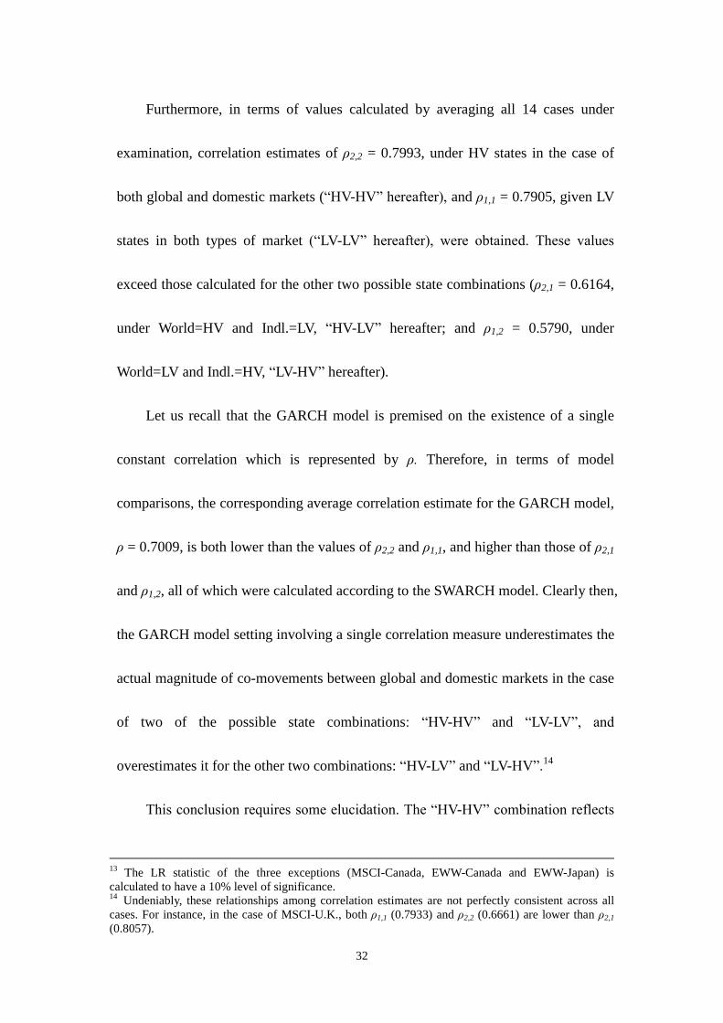
Furthermore, in terms of values calculated by averaging all 14 cases under

examination, correlation estimates of ρ2,2 = 0.7993, under HV states in the case of

both global and domestic markets (“HV-HV” hereafter), andρ1,1 = 0.7905, given LV

states in both types of market (“LV-LV” hereafter), were obtained. These values

exceed those calculated for the other two possible state combinations (ρ2,1 = 0.6164,

under World=HV and Indl.=LV, “HV-LV”hereafter; and ρ1,2 = 0.5790, under

World=LV and Indl.=HV,“LV-HV”hereafter).

Let us recall that the GARCH model is premised on the existence of a single

constant correlation which is represented by ρ.Therefore, in terms of model

comparisons, the corresponding average correlation estimate for the GARCH model,

ρ= 0.7009, is both lower than the values ofρ2,2 andρ1,1, and higher than those ofρ2,1

andρ1,2, all of which were calculated according to the SWARCH model. Clearly then,

the GARCH model setting involving a single correlation measure underestimates the

actual magnitude of co-movements between global and domestic markets in the case

of two of the possible state combinations: “HV-HV” and “LV-LV”, and

overestimates it for the other two combinations:“HV-LV”and“LV-HV”.14

This conclusion requires some elucidation. The “HV-HV” combination reflects

13 The LR statistic of the three exceptions (MSCI-Canada, EWW-Canada and EWW-Japan) iscalculated to have a 10% level of significance.14 Undeniably, these relationships among correlation estimates are not perfectly consistent across allcases. For instance, in the case of MSCI-U.K., both ρ1,1 (0.7933) and ρ2,2 (0.6661) are lower than ρ2,1

(0.8057).

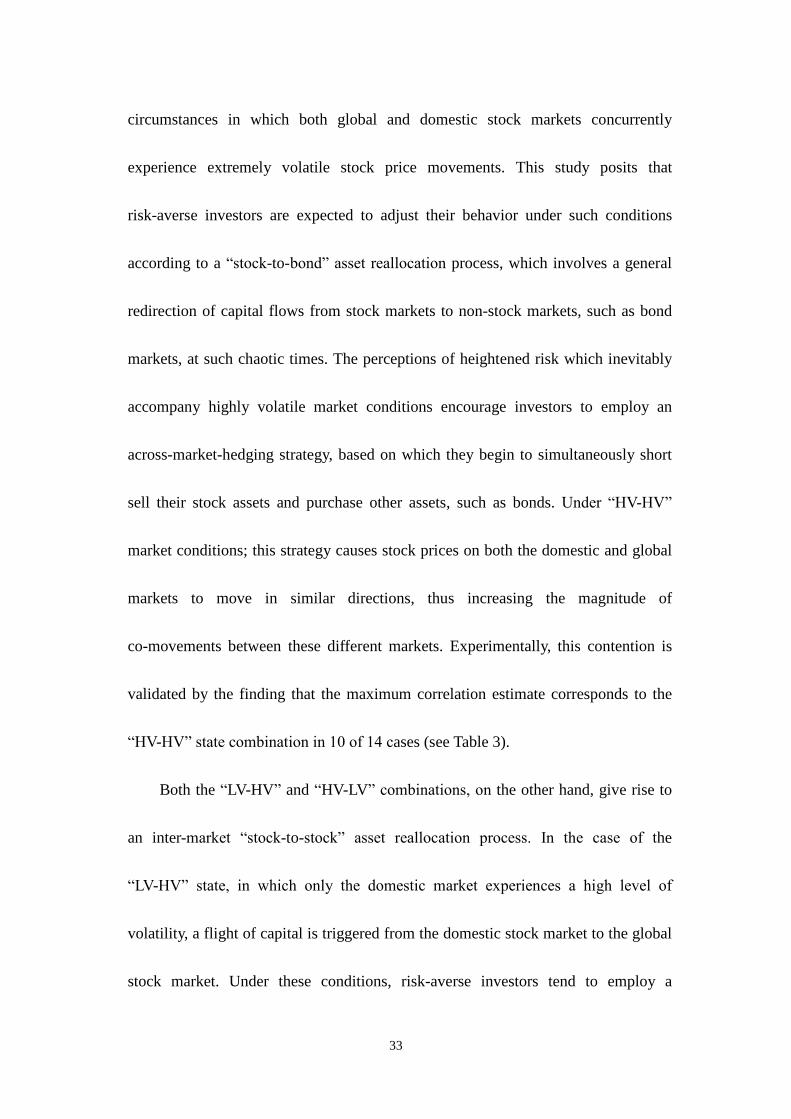
33

circumstances in which both global and domestic stock markets concurrently

experience extremely volatile stock price movements. This study posits that

risk-averse investors are expected to adjust their behavior under such conditions

according to a “stock-to-bond” asset reallocation process, which involves a general

redirection of capital flows from stock markets to non-stock markets, such as bond

markets, at such chaotic times. The perceptions of heightened risk which inevitably

accompany highly volatile market conditions encourage investors to employ an

across-market-hedging strategy, based on which they begin to simultaneously short

sell their stock assets and purchase other assets, such as bonds. Under “HV-HV”

market conditions; this strategy causes stock prices on both the domestic and global

markets to move in similar directions, thus increasing the magnitude of

co-movements between these different markets. Experimentally, this contention is

validated by the finding that the maximum correlation estimate corresponds to the

“HV-HV” state combination in 10 of 14 cases (see Table 3).

Both the “LV-HV”and “HV-LV” combinations, onthe other hand, give rise to

an inter-market “stock-to-stock” asset reallocation process. In the case of the

“LV-HV” state, in which only the domestic market experiences a high level of

volatility, a flight of capital is triggered from the domestic stock market to the global

stock market. Under these conditions, risk-averse investors tend to employ a

34

within-market-hedging strategy, which leads them to short sell their domestic stock

market assets, and to purchase global stock market assets in their place.

Consequently, stock prices on both the domestic and global markets move in

opposite directions, thus reducing the magnitude of co-movements between these

different markets. A similar line of reasoning can be applied to the “HV-LV”

combination. In this case, the domestic stock market presents relatively less risk;

accordingly, capital flows in the opposite direction towards the domestic stock

market. Furthermore, given that both the “stock-to-stock”asset reallocation process

and the underlying strategy are the same here as in the preceding case, a reduction in

the magnitude of cross-market correlations occurs.

To sum up, two asset reallocation processes have been described which are held

to explain variations in the strength of cross-market correlations existing under

different states of market volatility. Specifically, the “stock-to-bond”process is

primarily associated with the “HV-HV”state, and it considerably increases the

magnitude of inter-market co-movements. By contrast, in both the “LV-HV”and

“HV-LV” states, the strength of cross-market correlations is significantly reduced as

a result of the“stock-to-stock”reallocation process.

There remains a state combination which has not yet been addressed. In the

case of the “LV-LV” combination, both the domestic and global stock markets are

35

held to be relatively stable, thus presenting minimal risk to wary investors. Under

such conditions, the aforementioned asset reallocation processes are deemed

inapplicable because unnecessary. As a result, in terms of the analyses conducted in

this study, the value of the correlation estimate of the “LV-LV’ state is lower than

that of the “HV-HV” state and higher than that of both the “HV-LV” and “LV-HV”

states.

Finally, it must be noted that it is impossible to compare the SWARCH and

GARCH models by conventional LR statistical analyses because the models are not

strictly nested15. As a result, the AIC and Schwarz value statistics were applied to the

evaluation of relative model performance.16 The comparison of Tables 2 and 3

reveals that the bivariate SWARCH model outperforms the bivariate GARCH model

in all cases in terms of these two measures of statistical effectiveness.

3.3 Asset Allocation Effectiveness: In-sample Tests

It is well known that the effectiveness of an international stock portfolio relies on

the prior careful consideration of a market specific factor, the level of variance within

both the domestic and global markets, and an inter-market factor, the strength with

which these different markets are correlated. If the weight attributed to each asset

15 The Markov-switching mechanism and the GARCH model are widely considered impossible tocombine, with the exception of Gray (1996), who established a system which permits such acombination on the basis of specific assumptions. See Hamilton and Susmel (1994) for a more in-depthdiscussion of this issue.16 See Schwarz (1978) for the Schwarz value and Akaike (1976) for AIC.

36

included in the portfolio is a function of both these factors, then obtaining accurate

correlation/variance measurements is obviously crucial. This study investigates the

feasibility of generating an international portfolio on the basis of state-varying

correlations. This possibility is put to the test in the context of different strategies for

the development of stock portfolios, one of which defines variance in relation to its

minimum level, whereas the other attributes to the variance a given value.

In the case of the first strategy, that is the design of a minimum variance portfolio

consisting of both domestic and world stock assets (See Eqs. 8 and 9), the in-sample

evaluation of the effectiveness of asset allocation strategies is detailed in Table 4.

These results indicate differences between portfolios designed according to either of

the models being studied; that is, the return mean for a SWARCH-based portfolio is

higher than that for a GARCH-based portfolio. However, although this difference is

prevalent, having been observed in 10 of 14 cases, it is statistically insignificant.17

Furthermore, the variance of the SWARCH-based portfolio is significantly lower (at a

1% level) than that of the GARCH-based portfolio in all cases18.

The annual return/risk (R/R) ratio of the GARCH-based portfolio is here used as

a benchmark against which is measured the degree to which the R/R ratio achieved by

17 The case of MSCI-Canada is exceptional in that the return mean for the GARCH-based portfolioexceeds that for the SWARCH-based portfolio at a 5% level of significance.18 Notably, this investigation devises a statistical test for examining whether the variances of theinternational portfolio varies significantly between using the bivariate GARCH and SWARCH models.Please see the appendix for the detail.

37

the SWARCH model can be deemed a success. As shown in panel (c) of Table 4, the

relative improvement of the R/R ratio in the case of the portfolio designed on the

basis of the SWARCH model suggests that the portfolio development strategy

involved is more effective than its GARCH-based counterpart (again with the

exception of MSCI-Canada).

The obvious conclusion is that the modeling of market correlations and

corresponding variances on the basis of variations in volatility states is both

statistically significant and strategically effective. Moreover, reductions in risk, rather

than increases in return mean, are to thank for the benefits stemming from such

improved effectiveness.

The second strategy under investigation proposes investing in a variety of

domestic and world assets to build a given variance portfolio (See Eqs. 10 and 11).

Table 5 presents the effectiveness of in-sample asset allocation based on this strategy.

As was true of the first strategy, the empirical results here indicate that the

SWARCH-based portfolio outperforms the GARCH-based portfolio in most cases. In

particular, the portfolio designed on the basis of the SWARCH model shows a relative

improvement of the R/R ratio in 10 of 14 cases.

3.4 Comparative Analysis across Various Volatility Regimes

The findings thus far demonstrate that the bivariate SWARCH model

38

considerably outperforms the GARCH model on the basis of general measures

encompassing the entire period concerned in this study. On the other hand, the related

question of how effectively the SWARCH model allocates stock assets during distinct

periods marked by differences in volatility remains unresolved.

In weekly increments, Fig. 1 depicts global and domestic market returns in the

illustrative case of MSCI-U.S., which manifest increased volatility at certain times.

Such findings warrant the use of the SWARCH model, which facilitates the

investigation of variance dynamics by methods of a jump process. In this way, the

unsettled issue mentioned above is addressed by the specific design of the SWARCH

model used in this study.

The specific volatility state existing at each point in time is here identified on the

basis of the estimation of the filtering probability of a particular state combination and

a maximum value criterion. For instance, if, at time t, the estimated filtering

probability of the “HV-HV” state combination (that is, st = 4, or sty = 2 and st

x = 2)

exceeds that of the three alternative states, then an “HV-HV” state is said to exist at

this point in time. SWARCH-based estimates of the filtering probabilities of specific

volatility state combinations for the illustrative case of MSCI-U.S. are shown in Fig. 2.

On a more general point, the market as a whole is here considered to be in a specific

state of volatility if the estimated filtering probability at any given time is relatively

39

high. Table 6 lists the observation percentage of return rates at which were observed

the different volatility state combinations. Appearing in 9 of 14 cases, the “LV-LV”

state is set as the maximum value.19

With the average standard errors calculated for both domestic and world assets

serving as benchmarks, the margin by which risk is reduced in the context of various

market volatility state combinations was assessed. The portfolio on which were based

the observations consists of equally weighted domestic and global assets. The results,

presented in Table 7, reveal that the “HV-HV” state combination represents the

minimum value in 10 of 14 cases. Furthermore, attempts at determining the extent to

which reductions in risk stemming from the international diversification of an

investment portfolio are beneficial are likely to overestimate the advantages perceived

in the case of an “HV-HV” state combination and underestimate them in the other

cases.

Attention must be brought to the fact that the “HV-HV” state combination

corresponds to both the least effective conditions under which risk is reduced by

international portfolio diversification, and the context in which the strongest market

return correlations exist (in terms of the value ofρ2,2; see Table 3).20 This observation

19 This finding is consistent with the notion that the LV state is more persistent than the HV state. Thispoint is illustrated in Table 3, where the values of py

11/px11 generally exceed those of py

22/px22.

20 The finding according to which the “HV-HV” state is associated with the smallest reduction in the level of risk is quite consistent, with the exception of MSCI-Italy, for which the value ofρ2,2 is secondto last.

40

suggests that setting a model with a single, constant correlation value is likely to

underestimate the actual strength of cross-market correlations and to overestimate the

effects of risk reduction under conditions of an “HV-HV” state combination.

The “HV-HV” state combination is thus shown to frequently be the context in

which the cross-market correlation is strongest. This phenomenon is supported by

factual evidence. On the one hand, volatility in global markets consistently coincides

with global financial or economic crises. On the other hand, a recession has been

shown to precede high levels of volatility in domestic markets (Chen, Roll and Ross,

1986; Schwert, 1990; Chen, 1991; Hamilton and Lin, 1996). At times when both

global crises and domestic recessions coincide, this study contends that the influence

of shared factors related to the world market dominate that of the idiosyncratic factors

characterizing domestic markets. Consequently, cross-market correlations rise

dramatically under such circumstances.

Estimates of risk reduction further serve as a basis for comparing the relative

performance of the GARCH and SWARCH models evaluated in this study.

Underlying this comparison is the variance of a GARCH-based portfolio, providing a

benchmark against which can be measured the extent to which a SWARCH-based

portfolio is successful at reducing investment risk. The resultant differences

(expressed in percentages), implicit in Table 8, make it possible for the effectiveness

41

of both models at reducing risk to be contrasted in the context of various volatility

state combinations. Table 8 also suggests a further comparison on the basis of the type

of portfolio considered; that is, panel (a) lists effectiveness ratings in the case of a

minimum variance portfolio, whereas panel (b) does the same for a given variance

portfolio.

In terms of risk reduction effectiveness, a general impression of the performance

of domestic stock market assets under conditions of low variance can be got from the

integration of the “HV-LV” and “LV-LV” state combinations listed in both panels of

Table 8. Therefore, by averaging all 14 cases in panel (a), the SWARCH model is

shown to be 13.48% more effective than the GARCH model at reducing risk in the

“HV-LV” state, and 7.21% more effective in the “LV-LV” state. In contrast, the

integration of the “HV-HV” and “LV-HV” state combinations reflects how domestic

markets react to conditions of high variance. Again, the SWARCH model proves

effective at reducing risk both in the “HV-HV” (6.79%) and the “LV-HV” (5.10%)

states.

Based on these observations, the largest reductions in investment risk result from

the global market being in a state of high volatility, regardless of whether the level of

the concurrent volatility of domestic markets is high or low. This conclusion suggests

that a state-varying framework is the most effective methods of diversifying an

42

investment portfolio in the context of a highly volatile global market.21

This study further investigates the optimization of the loading of a portfolio in

terms of time variation. To this end, the standard error of the portfolio weights

determined on the basis of the SWARCH model is divided by that for the GARCH

model to calculate a relative measure of time variation in loading optimization (see

Table 9). In evaluating the results, a value lower than unity suggests that portfolio

loadings determined on the basis of the SWARCH model are less volatile than those

derived from the GARCH model, whereas a higher such volatility level results from a

value higher than unity.

Panel (a) of Table 9 presents the results of the analysis of a minimum variance

portfolio consisting of both domestic and global assets. The examination of the period

under investigation as a whole reveals that the measures of relative time variation

exceed unity in 13 of 14 cases. However, when different combinations of volatility

states are taken into account, SWARCH-based portfolio loadings are stabilized to a

considerable extent, particularly in the “HV-HV” state, where the relative time

variation falls below unity in 10 of 14 cases.22

Fig. 3 depicts the optimal loading of a minimum variance portfolio with global

stock market assets in the illustrative case of MSCI-U.K. According to this figure, the

21 This conclusion remains valid when a similar analysis of the data for a given variance portfolio isperformed (see panel (b) of Table 8).22 Furthermore, our analyses show that the relative time variation falls below unity in 5 of 14 cases inthe “LV-LV” state, 6 of 14 in the “HV-LV” state, and 3 of 14in the “LV-HV” state.

43

GARCH model frequently produces a corner solution; that is, it accounts for 100% of

global asset loadings. This observation explains why GARCH-generated portfolio

loadings tend to be more stable than those produced by the SWARCH model.

However, SWARCH-based portfolio loadings stabilize, in the case of the “HV-HV”

state in particular, after structural changes in the volatility of returns have been

filtered out. In contrast, the conventional GARCH model with a time-varying

parameter fails to account for structural changes in return variance dynamics.

Therefore, it generates hedge ratio estimates with greater time variation, particularly

in times marked by the “HV-HV” state.

Because the strategy for the development of an investment portfolio based on the

setting of a minimum level of variance repeatedly produces a corner solution, the

alternative strategy of fixing the variance at a given level is here considered. The

optimal portfolio loading corresponding to this alternative strategy for the illustrate

case of MSCI-U.K. is depicted in Fig. 4, which shows a sizable decrease in the

frequency of GARCH-produced corner solutions. Furthermore, the portfolio loading

determined on the basis of the SWARCH model appears to be much more stable than

that generated by the GARCH model. This finding of the greater stability of the

SWARCH model in the case of a given variance portfolio is further validated by the

findings listed in panel (b) of Table 9. In the case of data covering the period under

44

observation as a whole, the relative time variation is below unity in 10 of 14 cases.23

There are practical implications to the findings reported in this section. The

higher levels of time variation associated with certain portfolio loading strategies

imply that the holders of such portfolios must frequently reposition their investments,

thus incurring higher transaction costs. Such strategies are here considered a direct

consequence of the failure of the GARCH model to account for structural changes in

return variance dynamics. Furthermore, investors opting for a GARCH-inspired

strategy for the diversification of their investment portfolios must cope with a

relatively ineffective asset allocation in addition to the extra transaction costs

mentioned above.

On the other hand, it was demonstrated that filtering out the structural dynamics

underlying volatility switching by the SWARCH model considerably decreases time

variation. This finding leads to the conclusion that the determination of portfolio

loadings based on the consideration of variations in volatility states corrects the

shortcomings inherent in the GARCH model, thus implying a more effective

allocation of assets and lower transaction costs.

3.5 Asset Allocation Effectiveness: Out-of-Sample Test

The relative effectiveness of two models in the design of strategies for the

23 Furthermore, the relative time variation is lower than unity in 5 of 14 cases in the “LV-LV” state, in12 of 14 in the “HV-LV” state, in 6 of 14 in the “LV-HV” state,and in 10 of 14 in the “HV-HV” state.

45

international diversification of investment portfolios has so far been evaluated on the

basis of historical data. However, the primary concern of investors lies in determining

the likelihood of the future success of alternative portfolio development models. In an

attempt to resolve this apparent contradiction, this study further evaluates the

effectiveness of asset allocation strategies by out-of-sample tests using the

rolling-estimation technique.24

According to the requirements of this technique, the final 200 weekly

observations of the sample (representing approximately four-year’s worth ofdata)

were omitted from the initial sample, and formed the sequential inputs of the rolling

estimation. The following is a more detailed description of how this technique is

carried out.

To begin with, at time t, 1,226 (equal to 1,426 minus 200) historical data are

incorporated into the estimation of the model parameters25, which is carried out on the

basis of 226,1

1, ix

ityit rr . The ex ante regime probabilities are then estimated, to be used

in the determination of the portfolio weights in the case of each volatility state. At

time t+1, a multi-step procedure based on the state-varying SWARCH model is

24 The out-of-sample tests conducted in this study resemble those reported by West, Edison and Cho(1993).25 How far back it is necessary to go when using historical data in model estimation presents somedifficulties in the field of portfolio management, and involves a trade-off between the quantity and thefreshness of the information submitted to analyses. This study contends that estimations based onsamples of limited size are less accurate because there is less chance of encountering data reflecting therarer, more extreme market movements that are associated with the greatest losses. Consequently, thenonlinear SWARCH model used here requires the inclusion of much data and is thus more likely toaccount for such rare and extreme behavior.

46

employed to determine the optimal portfolio loadings. First, the estimation of the

regime probabilities at time t+1 is carried out on the basis of population parameters

which were estimated at time t, t

. The one-step-ahead forecasts thus derived are

then used to determine the loading of a SWARCH-based portfolio at time t+1.26

With the addition of each subsequent observation, the same multi-step procedure

is repeated. Furthermore, following each such addition, the sample is rolled; that is,

the deliberate deletion of the oldest observation coincides with the addition of the

most recent one. This technique thus fixes the sample size at 1,226 observations.

In the case of a minimum variance portfolio consisting of both domestic and

world stock assets, the out-of-sample evaluation of the effectiveness of asset

allocation strategies is detailed in Table 10. The corresponding comparative analysis

of the two models was performed on six selected cases.27 Contrary to expectations,

however, the SWARCH model underperforms the GARCH model in most cases.

More specifically, the variance of the SWARCH-based portfolio is higher than that of

its GARCH-based counterpart in 5 of 6 cases, and it is significantly so in two

instances. In line with such findings, the R/R ratio of the portfolio designed on the

basis of the SWARCH model actually decreases in relation to the GARCH

26 To facilitate the process of convergence, this study uses the estimate for a given individual period asthe initial value in the non-linear estimation of the period immediately following it.27 As is well known, estimations carried on the basis of the non-linear SWARCH model aretime-consuming. In order to economize time, the out-of-sample test presented in this study isperformed on six cases only.

47

benchmark.

Fig. 5 depicts regime probability forecasts derived on the basis of the SWARCH

model in the illustrative case of MSCI-Japan.28 Thus, the likelihood of the different

volatility state combinations occurring is predicted. Fig. 6 also consists of results in

the case of MSCI-Japan. Specifically, GARCH-derived estimates of the rolling

loadings of a portfolio with global assets are presented in Fig. 6(a), whereas those

based on the SWARCH model are presented in Fig. 6(b). As was observed in the case

of Fig. 3 above, Fig. 6 suggests that the GARCH model seems to frequently produce a

corner solution during the process of conducting rolling estimations. This observation

partially explains the relatively poor performance of the SWARCH model in the

context of the out-of-sample testing of a minimum variance portfolio.

Turning now to the diversification of a given variance portfolio, Table 11

describes the effectiveness of out-of-sample asset allocation. Close examination of

these results shows them to be the diametrical opposite of those for the minimum

variance portfolio. First, a comparative analysis reveals the SWARCH model to be

more effective than the GARCH model in most cases. In particular, the mean return

for a SWARCH-based portfolio is higher than that for a GARCH-based portfolio in all

selected cases.29 Furthermore, the variance of the SWARCH-based portfolio is lower

28 In the case of a SWARCH-based portfolio, the relative improvement of the R/R ratio forMSCI-Japan is the smallest among the six cases under investigation here.29 Note that only one of them is significant at the 5% level.

48

than that of the GARCH-based in 5 of 6 cases, and it is significantly so in three

instances. Further evidence of the superior performance of the SWARCH model is

provided by the finding that the R/R ratio of the portfolio designed on the basis of the

SWARCH model shows improvement in relation to the GARCH benchmark in all six

cases.

Again using MSCI-Japan as an illustrative case, Fig. 7(a) shows estimates of the

rolling loadings of a given variance portfolio with global assets derived by the

GARCH model; those based on the SWARCH model are presented in Fig. 7(b).

According to the results depicted in Fig. 7, it would appear that using a given level of

variance as a target on which to base portfolio design decision-making effectively

reduces the likelihood of producing corner solutions, which in turn corresponds to the

increased relative effectiveness of asset allocation strategies derived on the basis of

the SWARCH model.

49

4. Conclusions and Future Research Directions

On the basis of a Markov-switching technique, this study analyzes the dynamics

underlying the cross-market correlations existing between domestic and global stock

markets. Various combinations of high/low volatility states characterizing both types

of markets are examined with the aim, first, of investigating how variations in such

correlations correspond to changes in combined volatility states, and, second, of

identifying the most effective strategy for determining optimal portfolio loadings.

The following conclusions are drawn on the basis of the analyses carried out in

this study.

First, the domestic and global markets are more strongly correlated when both

simultaneously find themselves in the same state of volatility (i.e., “HV-HV” and

“LV-LV”). Conversely, this correlation is weaker when a different volatility state

characterizes each market (i.e., “LV-HV” and “HV-LV”). Furthermore, the

circumstances in which both the domestic and global stock markets are

simultaneously being disrupted by high levels of volatility (i.e., “HV-HV”) , on the

one hand, prove least effective at reducing the risk stemming from international

portfolio diversification, and, on the other, result in the strongest cross-market

correlations.

Second, the determination of optimal portfolio loadings according to a

50

state-varying framework proves a highly effective strategy for the allocation of assets,

and this due to reductions in risk, rather than increases in mean returns, thus produced.

This framework is fleshed out in the form of a SWARCH model, the overall superior

performance of which is demonstrated by conducting in-sample tests, although

out-of-sample testing shows the relative performance of the SWARCH model to be

less promising, especially where corner solutions are concerned. On a related point,

filtering structural changes in the volatility of returns out from the variance-switching

process leads to a considerable decrease of the time variation involved in generating

state-varying portfolio loadings. These reductions in time variation result in lower

transaction costs when they fall below the level of the time variation involved in

generating conventional time-varying loadings,.

In light of certain limitations of this study, the following are suggestions for

future research.

First, the observations are made exclusively on data from the stock markets of

G7 countries, thus severely limiting their generalizability. Future studies could

examine a range of stock markets, especially emerging stock markets. Specifically,

this suitability of the Markov-switching system rests on its sensitivity to rare and

extreme price fluctuations to which emerging stock markets are much more prone

than mature stock markets are. Therefore, it would be useful to conduct a comparative

51

analysis of mature and emerging stock markets.

Second, two alternative strategies for the determination of the loading of an

internationally diversified stock portfolio (i.e. state-varying loading implied by the

SWARCH model and time-varying loading obtained from the GARCH model) are

evaluated both independently and comparatively. However, it would be useful to carry

out comparisons of these approaches with other models based on different portfolio

loading designs. Finally, two variance targets are incorporated into the models studied,

but other such targets could be used to reexamine the extent to which state-varying

portfolio designs are effective at asset allocation.

52

Appendix

To examine the variances of international portfolio varies significantly between

using the bivariate GARCH and SWARCH models; this investigation devises a

statistical test as below. First, this study calculates the returns of international

portfolio involving domestic and world market assets for each period, as follows:

Ttrwrwr xt

GARCHxt

yt

GARCHyt

GARCHt ,,...1,,, (1)

Ttrwrwr xt

SWARCHxt

yt

SWARCHyt

SWARCHt ,,...1,,, (2)

,where rty and rt

x represent return rates of global and domestic markets, respectively.

Additionally, GARCHytw , and GARCHx

tw , ( SWARCHytw , and SWARCHx

tw , ) are the optimal

portfolio loadings established by the bivariate GARCH (SWARCH) model, and

GARCHtr ( SWARCH

tr ) are the corresponding return rates of international portfolio. Next,

the sample variances of the two return rates: )( GARCHrVAR for GARCHtr and

)( SWARCHrVAR for SWARCHtr , are calculated, respectively.

The test mainly examines whether the difference of the two variances,

)()( SWARCHGARCH rVARrVAR significantly exceeds zero. Owing to the mean value of

daily stock returns being very close to zero, this study simplifies the difference

between the two variances as follows:

53

])[(])[( 22 SWARCHGARCH rErE (3)

Furthermore, the above equation is rewritten as follows:

)])([(

])()[(

])[(])[(22

22

SWARCHGARCHSWARCHGARCH

SWARCHGARCH

SWARCHGARCH

rrrrE

rrE

rErE

(4)

Clearly, to test if the difference of two variances is significantly greater than 0 equals

test if the correlation coefficient between two return rates: )( SWARCHGARCH rr and

)( SWARCHGARCH rr is significantly exceeding 0. To achieve this, this study calculates

the following two return rates: SWGtr

and SWGtr

, as follows:

Ttrrr SWARCHt

GARCHt

SWGt ,...,1, (5)

Ttrrr SWARCHt

GARCHt

SWGt ,...,1, (6)

To test the significance of the correlation coefficient between SWGtr

and SWGtr

,

this investigation establishes a d statistic, as follows:

54

)(

)()/1(1

SWGt

SWGt

SWGt

T

t

SWGt

rrSD

rrTTd

(7)

, where the

T

t

SWGt

SWGt rrT

1

)()/1( and )( SWGt

SWGt rrSD are the sample mean

and standard error estimate of the cross return rates, )( SWGt

SWGt rr , respectively.

Furthermore, under the central limit theorem, the d statistic exhibits a standard normal

distribution.

55

ReferencesAng, A. and Bekaert, G. (2002) International asset allocation with regime shifts,

Review of Financial Studies, 15, 1137-1187Bae, K. H., Karolyi, G. A. and Stulz, R. M. (2003) A New Approach to Measuring

Financial Contagion, Review of Financial Studies, 16, 717-763Baillie, R. T., and Bollerslev, T. (1990) A multivariate generalized ARCH approach to

modeling risk premia in the forward foreign exchange rate, Journal ofInternational Money and Finance, 9, 309-324

Bollerslev, T. (1986) Generalized autoregressive conditional heteroskedasticity,Journal of Econometrics, 31, 307-327

Bollerslev, T. and Engle, R. F. (1986) Modeling the persistence of conditionalvariance, Econometric Reviews, 5, 1-50

Bollerslev, T. (1990) Modelling the coherence in short-run nominal exchange rates: Amultivariate generalized ARCH model, Review of Economics and Statistics, 72,498-505

Bollerslev, T., Chou, R. Y. and Kroner, K. F. (1992) ARCH modeling finance: Areview of the theory and empirical evidence, Journal of Econometrics, 52, 5-59

Boyer, B. H., Gibson, M. S. and Loretan, M. (1999) Pitfalls in test for changes incorrelations, International Finance Discussion Paper, no. 597, Federal ReserveBoard

Byers, J. D. and Peel, D. A. (1993) Some evidence on the interdependence of nationalstock markets and the gains from international portfolio diversification, AppliedFinancial Economics, 3, 239-242

Chan, K., Chan, K. C. and Karolyi, A. G. (1991) Intraday volatility in the stock indexand stock index futures markets, Review of Financial Studies, 4, 657-684

Chang, T. (2001) Are there any long-run benefits from international equitydiversification for Taiwan investors diversifying in the equity markets of its majortrading partners, Hong Kong, Japan, South Korea, Thailand and the USA, AppliedEconomics Letters, 8, 441-446

Chen, N. F. (1991) Financial investment opportunities and the macroeconomy,Journal of Finance, 46, 529-554

Chen, N. F., Roll, R. and Ross, S. A. (1986) Economic forces and the stock market,Journal of Business, 56, 383-403

Das, S. R. and Uppal, R. (2004), Systemic risk and international portfolio choice,Journal of Finance, 59, 2809-2834

Diebold, F. X. (1986) Modeling the persistence of conditional variance: A comment,Econometric Reviews, 5, 51-56

Edwards, S. and Susmel, R. (2003) Interest-rate volatility in emerging markets,

56

Review of Economics and Statistics, 85,328-348Engel, R. F. (1982) Autoregressive conditional heteroscedasticity with estimates of

variance of United Kingdom inflation, Econometrica, 50, 987-1007Engle, R. F. and Mustafa, C. (1992) Implied ARCH models from options prices,

Journal of Econometrics, 52, 289-311Erb, C. B., Harvey, C. R. and Viskanta, T. E. (1994) Forecasting international equity

correlations, Financial Analysts Journal, 50, 32-45Fernandez-Serrano, J. L. and Sosvilla-Rivero, S. (2003) Modelling the linkages

between US and Latin American stock markets, Applied Economics, 35,1423-1434

Fifield, S. G. M., Power, D. M. and Sinclair, C. D. (2002) Emerging stock markets: Amore realistic assessment of the gains from diversification, Applied FinancialEconomics, 12, 213-229

Forbes, K. J. and Rigobon, R. (2002) No contagion, only interdependence: measuringstock market co-movement, Journal of Finance, 57, 2223-2261

French, K. R. and Poterba, J. M. (1991) Investor diversification and internationalequity markets, American Economic Review, 81, 222-226

Gray, S. F. (1996) Modeling the conditional distribution of interest rates as aregime-switching process, Journal of Financial Economics, 42, 27-62

Hamilton, J. D. and Lin, G. (1996) Stock market volatility and the business cycle,Journal of Applied Econometrics, 11, 573-593

Hamilton, J. D. and Susmel R. (1994) Autoregressive conditional heteroscedasticityand changes in regime, Journal of Econometrics, 64, 307-333

Heimonen, K. (2002) Stock market integration: Evidence on price integration andreturn convergence, Applied Financial Economics, 12, 415-429

Jacquier, E. and Marcus, A. J. (2001) Asset allocation models and market volatility,Financial Analysts Journal, 57, 16-31

Karolyi, G. A. and Stulz, R. M. (1996) Why do markets move together? Aninvestigation of US-Japan stock return comovements, Journal of Finance, 3,951-986

Kempa, B. and Nelles, M. (2001) International correlations and excess returns inEuropean stock markets: Does EMU matter? Applied Financial Economics, 11,69-73

King, M. A. and Wadhwanl, S. (1990) Transmission of volatility between stockMarkets, Review of Financial Studies, 3, 5-33

Lamoureux, C. G. and Lastrapes, W. D. (1990), Persistence in variance, structuralchange and the GARCH model, Journal of Business and Economic Statistics, 8,225-234

57

Li, M. Y. and Lin, H. W. (2003) Examining the volatility of Taiwan stock indexreturns via a three-volatility-regime Markov-switching ARCH model, Review ofQuantitative Finance and Accounting, 21, 123-139

Lin, W.-L., Engle, R. F. and Ito, T. (1994) Do bulls and bears move across borders?International transmission of stock returns and volatility, Review of FinancialStudies, 7, 507-538

Longin, F. and Solnik, M. B. (1995) Is the correlation on international equity returnsconstant: 1960-1990, Journal of international Money and Finance, 14, 3-23

Longin, F. and Solnik, M. B. (2001) Extreme correlation of international equitymarkets, Journal of Finance, 56, 649-676

Luenberger, D. G. (1984) Linear and nonlinear programming, Reading, MA:Addison-Wesley

Nelson, D. B. (1991) Conditional heteroskedasticity in asset returns: a new approach,Econometrica, 59, 347-370

Ramchand, L. and Susmel, R. (1998) Volatility and cross correlation across majorstock markets, Journal of Empirical Finance, 5, 397-416

Roll, R. (1988) The international crash of October 1987, Financial Analysts Journal,44, 19-37

Schwert, G. W. (1990) Stock returns and real activity: a century of evidence, Journalof Finance, 45, 1237-1257

Schwert, G. W. and Seguin, P. J. (1990) Heteroskedasticity in stock returns, Journal ofFinance, 45, 1129-1155

Syriopoulos, T. (2004) International portfolio diversification to central European stockmarkets, Applied Financial Economics, 14, 1253-1268

Tahai, A., Rutledge, R. W. and Karim, K. E. (2004) An examination of financialintegration for the group of seven (G7) industrialized countries using an I(2)cointegration model, Applied Financial Economics, 14, 327-335

Tesar, L. L. and Werner, I. (1992) Home bias and the globalization of securitiesmarkets, NBER Working Paper, No. 4218, National Bureau of Economic Research,Cambridge, MA

West, K. D., Edison, H. J. and Cho, D. (1993) A utility-based comparison of somemodels of exchange rate volatility, Journal of International Economics, 35, 23-45

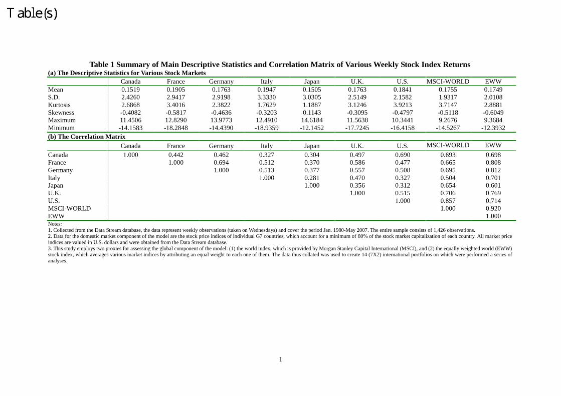
1

Table 1 Summary of Main Descriptive Statistics and Correlation Matrix of Various Weekly Stock Index Returns(a) The Descriptive Statistics for Various Stock Markets

Canada France Germany Italy Japan U.K. U.S. MSCI-WORLD EWWMean 0.1519 0.1905 0.1763 0.1947 0.1505 0.1763 0.1841 0.1755 0.1749S.D. 2.4260 2.9417 2.9198 3.3330 3.0305 2.5149 2.1582 1.9317 2.0108Kurtosis 2.6868 3.4016 2.3822 1.7629 1.1887 3.1246 3.9213 3.7147 2.8881Skewness -0.4082 -0.5817 -0.4636 -0.3203 0.1143 -0.3095 -0.4797 -0.5118 -0.6049Maximum 11.4506 12.8290 13.9773 12.4910 14.6184 11.5638 10.3441 9.2676 9.3684Minimum -14.1583 -18.2848 -14.4390 -18.9359 -12.1452 -17.7245 -16.4158 -14.5267 -12.3932(b) The Correlation Matrix

Canada France Germany Italy Japan U.K. U.S. MSCI-WORLD EWWCanada 1.000 0.442 0.462 0.327 0.304 0.497 0.690 0.693 0.698France 1.000 0.694 0.512 0.370 0.586 0.477 0.665 0.808Germany 1.000 0.513 0.377 0.557 0.508 0.695 0.812Italy 1.000 0.281 0.470 0.327 0.504 0.701Japan 1.000 0.356 0.312 0.654 0.601U.K. 1.000 0.515 0.706 0.769U.S. 1.000 0.857 0.714MSCI-WORLD 1.000 0.920EWW 1.000Notes:1. Collected from the Data Stream database, the data represent weekly observations (taken on Wednesdays) and cover the period Jan. 1980-May 2007. The entire sample consists of 1,426 observations.2. Data for the domestic market component of the model are the stock price indices of individual G7 countries, which account for a minimum of 80% of the stock market capitalization of each country. All market priceindices are valued in U.S. dollars and were obtained from the Data Stream database.3. This study employs two proxies for assessing the global component of the model: (1) the world index, which is provided by Morgan Stanley Capital International (MSCI), and (2) the equally weighted world (EWW)stock index, which averages various market indices by attributing an equal weight to each one of them. The data thus collated was used to create 14 (7X2) international portfolios on which were performed a series ofanalyses.

2

Table 2 Parameter Estimates of the Bivariate GARCH Model with One Single Correlation(a) MSCI World Index -G7 Stock Markets

MSCI-Canada MSCI-France MSCI-Germany MSCI-Italy MSCI-Japan MSCI-U.K. MSCI-U.S.World Market Eq.

θy0 0.2294 (0.0435)*** 0.2365 (0.0440)*** 0.2018 (0.0446)*** 0.2108 (0.0449)*** 0.2630 (0.0458)*** 0.2075 (0.0444)*** 0.2171 (0.0456)***

θy1 -0.0100 (0.0140) -0.0214 (0.0246) -0.0062 (0.0413) -0.0082 (0.0240) -0.0466 (0.0256)* 0.0134 (0.0158) 0.0145 (0.0265)

αy0 0.2055 (0.0469)*** 0.1592 (0.0358)*** 0.2520 (0.0520)*** 0.1923 (0.0451)*** 0.2429 (0.0525)*** 0.1391 (0.0342)*** 0.2276 (0.0437)***

αy1 0.0940 (0.0138)*** 0.0861 (0.0119)*** 0.0906 (0.0132)*** 0.1013 (0.0141)*** 0.1141 (0.0148)*** 0.0908 (0.0125)*** 0.0706 (0.0101)***

βy1 0.8518 (0.0203)*** 0.8729 (0.0155)*** 0.8405 (0.0203)*** 0.8496 (0.0185)*** 0.8237 (0.0217)*** 0.8752 (0.0165)*** 0.8656 (0.0168)***

Individual Market Eq.θx

0 0.2138 (0.0567)*** 0.3097 (0.0665)*** 0.2334 (0.0647)*** 0.1991 (0.0760)*** 0.2470 (0.0732)*** 0.2274 (0.0590)*** 0.2197 (0.0496)***θx

1 0.0751 (0.0235)*** -0.0618 (0.0252)*** 0.0100 (0.0226) 0.0239 (0.0307) 0.0291 (0.0229) -0.0253 (0.0223) -0.0574 (0.0245)***

αx0 1.2060 (0.2175)*** 0.5840 (0.1159)*** 0.4261 (0.0915)*** 0.2994 (0.0773)*** 0.6514 (0.1940)*** 0.3432 (0.0866)*** 0.2276 (0.0536)***

αx1 0.1431 (0.0222)*** 0.1278 (0.0177)*** 0.1001 (0.0145)*** 0.0863 (0.0134)*** 0.0936 (0.0186)*** 0.0937 (0.0129)*** 0.0649 (0.0096)***

βx1 0.6505 (0.0475)*** 0.8070 (0.0235)*** 0.8491 (0.0199)*** 0.8904 (0.0155)*** 0.8336 (0.0354)*** 0.8576 (0.0193)*** 0.8824 (0.0182)***

Correlationρ 0.6833 (0.0142)*** 0.6523 (0.0153)*** 0.6637 (0.0149)*** 0.5133 (0.0200)*** 0.6600 (0.0151)*** 0.7142 (0.0130)*** 0.8413 (0.0079)***

Log-lik. -5652.1071 -5938.0385 -5904.8489 -6318.9724 -6001.3949 -5652.7313 -5021.5015AIC value -5663.1071 -5949.0385 -5915.8489 -6329.9724 -6012.3949 -5663.7313 -5032.5015Schwarz value -5692.0516 -5977.9830 -5944.7934 -6358.9169 -6041.3394 -5692.6758 -5061.4460

(b) EWW World Index- G7 Stock Markets

EWW-Canada EWW-France EWW-Germany EWW-Italy EWW-Japan EWW-U.K. EWW-U.S.World Market Eq.

θy0 0.2367 (0.0490)*** 0.2581 (0.0475)*** 0.2102 (0.0502)*** 0.2184 (0.0468)*** 0.2651 (0.0475)*** 0.2107 (0.0494)*** 0.2346 (0.0497)***

θy1 0.0097 (0.0154) -0.0184 (0.0152) 0.0218 (0.0150) 0.0088 (0.0122) -0.0073 (0.0134) 0.0469 (0.0209)** 0.0186 (0.0203)

αy0 0.3838 (0.0984)*** 0.3858 (0.0771)*** 0.7670 (0.1767)*** 0.5418 (0.1043)*** 0.7030 (0.1707)*** 0.2816 (0.0547)** 0.4200 (0.0898)***

αy1 0.0948 (0.0178)*** 0.0717 (0.0117)*** 0.0809 (0.0157)*** 0.1153 (0.0183)*** 0.1359 (0.0244)*** 0.0886 (0.0130)*** 0.0837 (0.0144)***

βy1 0.8089 (0.0372)*** 0.8292 (0.0265)*** 0.7182 (0.0543)*** 0.7481 (0.0364)*** 0.6874 (0.0582)*** 0.8427 (0.0217)*** 0.8087 (0.0312)***

Individual Market Eq.θx

0 0.2144 (0.0608)*** 0.3151 (0.0662)*** 0.2344 (0.0690)*** 0.1972 (0.0729)*** 0.2363 (0.0705)*** 0.2113 (0.0610)*** 0.2291 (0.0491)***θx

1 0.0587 (0.0219)*** -0.0763 (0.0199)*** 0.0181 (0.0195) 0.0245 (0.0203) 0.0376 (0.0230) -0.0112 (0.0275) -0.0909 (0.0230)***αx

0 1.2171 (0.2268)*** 0.7318 (0.1396)*** 0.7150 (0.1529)*** 0.3265 (0.0743)*** 0.7281 (0.2064)*** 0.4395 (0.1242)*** 0.2519 (0.0662)***αx

1 0.1393 (0.0228)*** 0.1118 (0.0159)*** 0.0909 (0.0142)*** 0.0854 (0.0122)*** 0.1048 (0.0203)*** 0.0983 (0.0138)*** 0.0931 (0.0155)***

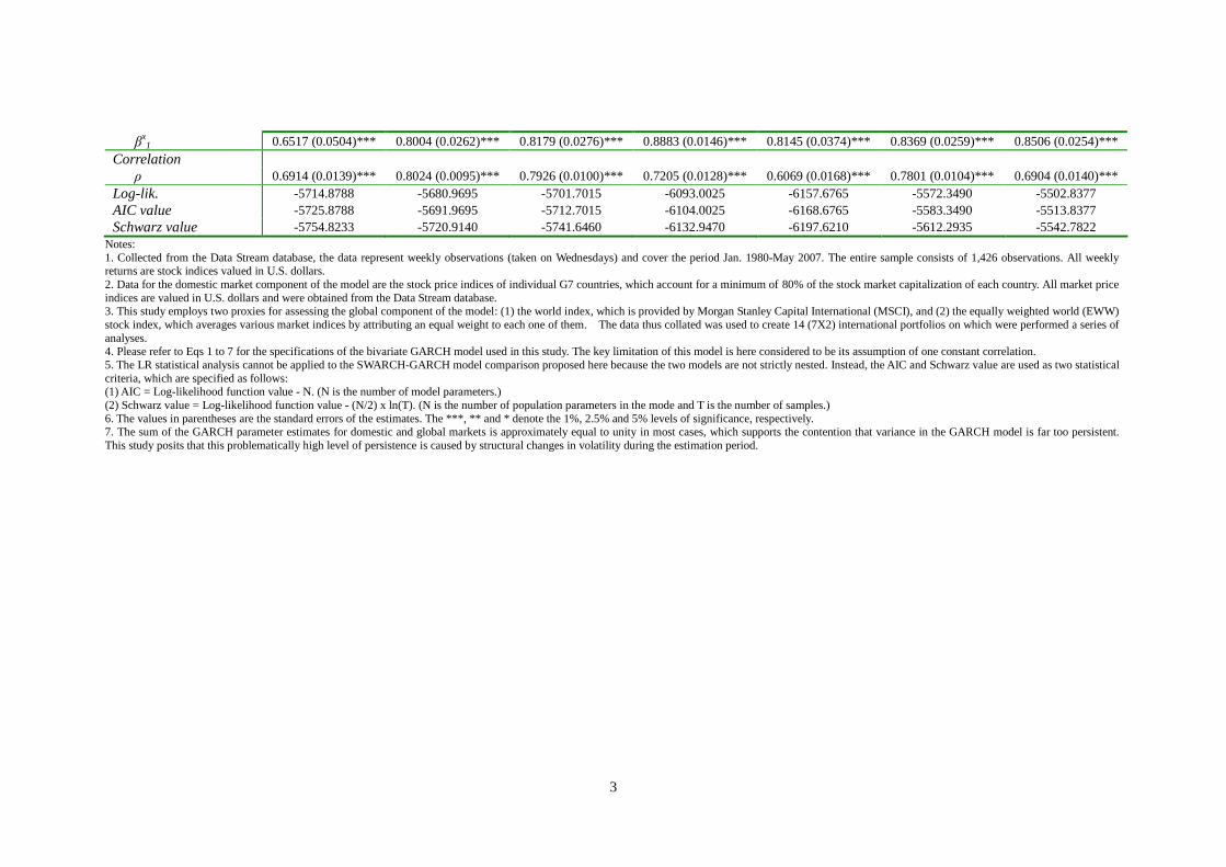
3

βx1 0.6517 (0.0504)*** 0.8004 (0.0262)*** 0.8179 (0.0276)*** 0.8883 (0.0146)*** 0.8145 (0.0374)*** 0.8369 (0.0259)*** 0.8506 (0.0254)***

Correlationρ 0.6914 (0.0139)*** 0.8024 (0.0095)*** 0.7926 (0.0100)*** 0.7205 (0.0128)*** 0.6069 (0.0168)*** 0.7801 (0.0104)*** 0.6904 (0.0140)***

Log-lik. -5714.8788 -5680.9695 -5701.7015 -6093.0025 -6157.6765 -5572.3490 -5502.8377AIC value -5725.8788 -5691.9695 -5712.7015 -6104.0025 -6168.6765 -5583.3490 -5513.8377Schwarz value -5754.8233 -5720.9140 -5741.6460 -6132.9470 -6197.6210 -5612.2935 -5542.7822

Notes:1. Collected from the Data Stream database, the data represent weekly observations (taken on Wednesdays) and cover the period Jan. 1980-May 2007. The entire sample consists of 1,426 observations. All weeklyreturns are stock indices valued in U.S. dollars.2. Data for the domestic market component of the model are the stock price indices of individual G7 countries, which account for a minimum of 80% of the stock market capitalization of each country. All market priceindices are valued in U.S. dollars and were obtained from the Data Stream database.3. This study employs two proxies for assessing the global component of the model: (1) the world index, which is provided by Morgan Stanley Capital International (MSCI), and (2) the equally weighted world (EWW)stock index, which averages various market indices by attributing an equal weight to each one of them. The data thus collated was used to create 14 (7X2) international portfolios on which were performed a series ofanalyses.4. Please refer to Eqs 1 to 7 for the specifications of the bivariate GARCH model used in this study. The key limitation of this model is here considered to be its assumption of one constant correlation.5. The LR statistical analysis cannot be applied to the SWARCH-GARCH model comparison proposed here because the two models are not strictly nested. Instead, the AIC and Schwarz value are used as two statisticalcriteria, which are specified as follows:(1) AIC = Log-likelihood function value - N. (N is the number of model parameters.)(2) Schwarz value = Log-likelihood function value - (N/2) x ln(T). (N is the number of population parameters in the mode and T is the number of samples.)6. The values in parentheses are the standard errors of the estimates. The ***, ** and * denote the 1%, 2.5% and 5% levels of significance, respectively.7. The sum of the GARCH parameter estimates for domestic and global markets is approximately equal to unity in most cases, which supports the contention that variance in the GARCH model is far too persistent.This study posits that this problematically high level of persistence is caused by structural changes in volatility during the estimation period.

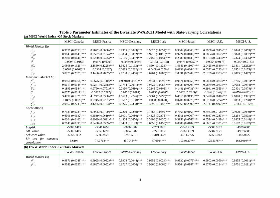
4

Table 3 Parameter Estimates of the Bivariate SWARCH Model with State-varying Correlations(a) MSCI World Index -G7 Stock Markets

MSCI-Canada MSCI-France MSCI-Germany MSCI-Italy MSCI-Japan MSCI-U.K. MSCI-U.S.World Market Eq.

py11 0.9856 (0.0053)*** 0.9822 (0.0060)*** 0.9905 (0.0043)*** 0.9825 (0.0057)*** 0.9804 (0.0063)*** 0.9908 (0.0045)*** 0.9848 (0.0053)***

py22 0.9643 (0.0140)*** 0.9507 (0.0184)*** 0.9834 (0.0062)*** 0.9716 (0.0115)*** 0.9724 (0.0106)*** 0.9854 (0.0072)*** 0.9828 (0.0057)***

θy0 0.2106 (0.0441)*** 0.2250 (0.0475)*** 0.2166 (0.0437)*** 0.2452 (0.0454)*** 0.2380 (0.0433)*** 0.2103 (0.0443)*** 0.2374 (0.0436)***

θy1 -0.0097 (0.0169) -0.0176 (0.0298) -0.0089 (0.0039) -0.0133 (0.0108) -0.0478 (0.0252)* -0.0054 (0.0178) -0.0004 (0.0183)

αy0 2.0808 (0.1326)*** 2.1850 (0.1225)*** 1.9625 (0.1193)*** 1.8504 (0.1126)*** 1.9683 (0.1109)*** 2.0425 (0.1530)*** 2.1811 (0.1262)***

αy1 0.0582 (0.0268)** 0.0324 (0.0237) 0.0683 (0.0232)*** 0.0408 (0.0250)* 0.0933 (0.0264)*** 0.0572 (0.0223)*** 0.0551 (0.0175)***

gy2 3.0975 (0.2875)*** 3.1460 (0.2887)*** 2.7738 (0.2466)*** 3.6264 (0.0285)*** 2.8331 (0.2409)*** 2.6289 (0.2333)*** 2.0875 (0.1472)***

Individual Market Eq.px

11 0.9864 (0.0054)*** 0.9675 (0.0110)*** 0.9891(0.0055)*** 0.9731 (0.0096)*** 0.9871 (0.0050)*** 0.9858 (0.0074)*** 0.9705 (0.0091)***px

22 0.9619 (0.0148)*** 0.9241 (0.0238)*** 0.9754 (0.0091)*** 0.9822 (0.0068)*** 0.9329 (0.0203)*** 0.9879 (0.0063)*** 0.9668 (0.0094)***θx

0 0.1893 (0.0544)*** 0.2790 (0.0701)*** 0.2390 (0.0680)*** 0.2145 (0.0805)*** 0.1481 (0.0731)*** 0.1941 (0.0565)*** 0.2401 (0.0474)***θx

1 0.0673 (0.0219)*** -0.0622 (0.0297)** 0.0126 (0.0182) 0.0136 (0.0285) 0.0432 (0.0245)* -0.0505 (0.0162)*** -0.0770 (0.0192)***

αx0 3.4797 (0.1926)*** 4.6742 (0.3360)*** 4.6673 (0.2746)*** 4.3561 (0.5295)*** 6.4515 (0.3135)*** 3.3470 (0.2640)*** 2.1870 (0.1371)***

αx1 0.0477 (0.0225)** 0.0745 (0.0267)*** 0.0517 (0.0188)*** 0.0080 (0.0231) 0.0786 (0.0275)*** 0.0758 (0.0234)*** 0.0853 (0.0208)***

gx2 2.9862 (0.2749)*** 3.1235 (0.3103)*** 2.9275 (0.2358)*** 3.3792 (0.4153)*** 3.0960 (0.2992)*** 2.3111 (0.2092)*** 2.4436 (0.1827)

Correlationsρ1,1 0.7135 (0.0235)*** 0.7905 (0.0190)*** 0.7260 (0.0289)*** 0.7363 (0.0392)*** 0.7666 (0.0168)*** 0.7933 (0.0198)*** 0.9079 (0.0099)***ρ2,1 0.6306 (0.0632)*** 0.5539 (0.0619)*** 0.5071 (0.0086)*** 0.4526 (0.2376)*** 0.4911 (0.0067)*** 0.8057 (0.0283)*** 0.5254 (0.0503)***ρ1,2 0.6204 (0.0460)*** 0.2929 (0.0691)*** 0.4308 (0.0650)*** 0.3408 (0.0430)*** 0.3958 (0.0766)*** 0.6524 (0.0419)*** 0.8835 (0.0148)***ρ2,2 0.7648 (0.0395)*** 0.8488 (0.0309)*** 0.8433 (0.0193)*** 0.6553 (0.0453)*** 0.8986 (0.0182)*** 0.6661 (0.0331)*** 0.9102 (0.0107)***

Log-lik. -5588.1415 -5841.6290 -5836.1382 -6253.7062 -5949.4139 -5589.9625 -4939.6985AIC value -5606.1415 -5859.6290 -5854.1382 -6271.7062 -5967.4139 -5607.9625 -4957.6985Schwarz value -5653.5052 -5906.9927 -5901.5019 -6319.0699 -6014.7776 -5655.3262 -5005.0622LR test for constantcorrelation 5.6104 74.9768*** 43.7948*** 47.6564*** 103.9620*** 125.5376*** 163.6060***

(b) EWW World Index -G7 Stock Markets

EWW-Canada EWW-France EWW-Germany EWW-Italy EWW-Japan EWW-U.K. EWW-U.S.World Market Eq.

py11 0.9871 (0.0048)*** 0.9925 (0.0032)*** 0.9908 (0.0044)*** 0.9952 (0.0024)*** 0.9832 (0.0073)*** 0.9902 (0.0060)*** 0.9855 (0.0061)***

py22 0.9641 (0.0137)*** 0.9897 (0.0052)*** 0.9727 (0.0076)*** 0.9860 (0.0068)*** 0.9564 (0.0187)*** 0.9775 (0.0124)*** 0.9751 (0.0111)***

5

θy0 0.2211 (0.0504)*** 0.2456 (0.0474)*** 0.2423 (0.0459)*** 0.2401 (0.0425)*** 0.2382 (0.0472)*** 0.2144 (0.0481)*** 0.2220 (0.0482)***

θy1 -0.0099 (0.0193) -0.0255 (0.0204) 0.0072 (0.0182) -0.0030 (0.0342) -0.0116 (0.0211) 0.0292 (0.0238) 0.0120 (0.0168)

αy0 2.4647 (0.1404)*** 2.5199 (0.1302)*** 2.6320 (0.1374)*** 2.5238 (0.1190)*** 2.3707 (0.1888)*** 2.4601 (0.1589)*** 2.4314 (0.1474)***

αy1 0.0622 (0.0225)*** 0.0500 (0.0161)*** 0.0837 (0.0199)*** 0.0767 (0.0198)*** 0.0938 (0.0280)*** 0.0570 (0.0222)*** 0.0684 (0.0219)***

gy2 2.6523 (0.2490)*** 2.2429 (0.1611)*** 1.9635 (0.1465)*** 2.9609 (0.2228)*** 2.8872 (0.3157)*** 2.5058 (0.2107)*** 2.2610 (0.1993)***

Individual Market Eq.px

11 0.9919 (0.0038)*** 0.9554 (0.0142)*** 0.9811 (0.0064)*** 0.9995 (0.0009)*** 0.9547 (0.0147)*** 0.9693 (0.0109)*** 0.9749 (0.0100)***px

22 0.9766 (0.0118)*** 0.9611 (0.0133)*** 0.9631 (0.0121)*** 0.9990 (0.0008)*** 0.9303 (0.0291)*** 0.9769 (0.0093)*** 0.9855 (0.0071)***θx

0 0.1781 (0.0593)*** 0.3105 (0.0644)*** 0.2948 (0.0634)*** 0.2596 (0.0661)*** 0.1395 (0.0726)*** 0.1932 (0.0571)*** 0.2239 (0.0470)***θx

1 0.0433 (0.0231)* -0.0946 (0.0216)*** -0.0060 (0.0144) 0.0119 (0.0238) 0.0446 (0.0260)* -0.0324 (0.0235) -0.0880 (0.0221)***

αx0 3.5470 (0.1995)*** 4.1555 (0.2595)*** 4.9475 (0.2698)*** 3.3589 (0.2530)*** 4.7705 (0.4269)*** 3.1981 (0.2440)*** 1.5658 (0.1250)***

αx1 0.0603 (0.0264)** 0.0939 (0.0222)*** 0.0718 (0.0198)*** 0.0564 (0.0175)*** 0.0212 (0.0503) 0.0789 (0.0234)*** 0.1113 (0.0283)***

gx2 2.9858 (0.2842)*** 2.4804 (0.1769)*** 2.5662 (0.1922)*** 3.4395 (0.2709)*** 3.1289 (0.3467)*** 2.3413 (0.1924)*** 3.3749 (0.2983)***

Correlationsρ1,1 0.7133 (0.0193)*** 0.9008 (0.0129)*** 0.8475 (0.0140)*** 0.8961 (0.0124)*** 0.6874 (0.0297)*** 0.8462 (0.0163)*** 0.7415 (0.0280)***ρ2,1 0.6379 (0.0436)*** 0.8255 (0.0291)*** 0.7639 (0.0303)*** 0.6380 (0.0827)*** 0.5398 (0.0616)*** 0.8607 (0.03080*** 0.3967 (0.1127)***ρ1,2 0.6784 (0.0452)*** 0.6212 (0.0322)*** 0.5703 (0.0416)*** 0.6240 (0.0186)*** 0.6148 (0.0437)*** 0.7114 (0.0240)*** 0.6693 (0.0316)***ρ2,2 0.7503 (0.0336)*** 0.9078 (0.0104)*** 0.9399 (0.0082)*** 0.8742 (0.0122)*** 0.6094 (0.0580)*** 0.7804 (0.0242)*** 0.7420 (0.0242)***

Log-lik. -5649.3655 -5567.0396 -5611.3108 -6017.0687 -6117.5955 -5512.0446 -5465.6024AIC value -5667.3655 -5585.0396 -5629.3108 -6035.0687 -6135.5955 -5530.0446 -5483.6024Schwarz value -5714.7292 -5632.4033 -5676.6745 -6082.4324 -6182.9592 -5577.4083 -5530.9661LR test for constantcorrelation 5.1524 124.6438*** 94.3840*** 77.9736*** 4.681 28.6032*** 11.9832***

Notes:1. Please refer to Eqs. 9 to 20 for the specifications of the bivariate SWARCH model used in this study. The key feature of this model is the fact that it is based on conducting 4-state correlation measurements.2. To test the null hypothesis of identical correlations, this bivariate SWARCH model is first estimated on the basis of 4-state correlations and L(HA), representing the log likelihood function. The model is thenestimated assuming the existence of a single constant correlation (ρ1,1=ρ2,1=ρ1,2=ρ2,2=ρ), which allows for the subsequent derivation of the log likelihood function of the restricted model, L(H0). Finally, this function isused to carry out a likelihood ratio test, LR=-2[L(H0)- L(HA)]. In terms of the null hypothesis, this test displays a χ2 distribution with 3 (= 4 - 1) degrees of freedom. Quite interestingly, the results of this LR statisticalanalysis make it possible to reject the null hypothesis at a 1% level of significance in most cases except those of MSCI-Canada, EWW-Canada and EWW-Japan, which are significant at the 10% level.3. The values in parentheses are the standard errors of the estimates. The ***, ** and * denote the 1%, 2.5% and 5% levels of significance, respectively.4. In terms of values calculated by averaging all 14 cases under examination, the calculated correlation estimates of ρ1,1 = 0.7799, under LV states in the case of both global domestic markets, and ρ2,2 = 0.6979, givenHV states in both types of markets, far exceed the estimates of the other two possible state combinations (ρ2,1 = 0.58414, World=HV and Indl.=LV; and ρ1,2 = 0.52491, World=LV and Indl.=HV). The averagecorrelation estimate for the GARCH model, ρ= 0.6582, is both lower than the values of ρ1,1 and ρ2,2, and higher than those of ρ2,1 and ρ1,2. The obvious conclusion is that the GARCH model setting of a singlecorrelation measure underestimates the actual magnitude of co-movements between global and domestic markets in the case of two of the possible state combinations (“LV-LV” and “HV-HV”), and overestimates it for the other two combinations (“LV-HV” and “HV-LV”).5. Other notations are consistent with Table 2.

6

Table 4 In-sample Asset Allocation Effectiveness of International Diversificationwith a Minimum Variance Portfolio of Domestic and World Assets

(a) Return MeanGARCH Model SWARCH Model Statistical Difference (GARCH-SWARCH)

MSCI WORLDCanada 0.1759 0.1604 1.7373*France 0.1685 0.1774 -0.9015Germany 0.1605 0.1591 0.1411Italy 0.1589 0.1682 -1.1579Japan 0.1627 0.1586 0.4412U.K. 0.1572 0.1667 -1.3622U.S. 0.1656 0.1730 -0.7340

EWW WORLDCanada 0.1639 0.1619 0.2209France 0.1714 0.1816 -1.3152Germany 0.1682 0.1683 -0.0143Italy 0.1707 0.1716 -0.3367Japan 0.1640 0.1718 -0.8209U.K. 0.1651 0.1694 -0.6910U.S. 0.1475 0.1569 -1.1011

(b) Return VarianceGARCH Model SWARCH Model Statistical Difference (GARCH-SWARCH)

MSCI WORLDCanada 3.5525 3.1963 6.8612***France 3.8200 3.3374 4.4507***Germany 3.7466 3.4071 3.8310***Italy 3.6771 3.3796 6.6110***Japan 3.6181 3.3743 4.7607***U.K. 3.6735 3.4329 6.6308***U.S. 3.6949 3.5091 5.0932***

EWW WORLDCanada 3.7418 3.3809 7.5922***France 4.0655 3.8929 2.9951***Germany 4.0868 3.9102 3.3885***Italy 4.0197 3.9700 3.7496***Japan 3.8776 3.4794 6.2138***U.K. 3.9684 3.7025 5.5099***U.S. 3.6563 3.3546 7.1799***

(c) Annual Return/Risk (R/R) Ratio

GARCH Model SWARCH Model R/R Ratio Improvement % of SWARCHagainst GARCH

MSCI WORLDCanada 0.6599 0.6344 -3.86%France 0.6096 0.6866 12.63%Germany 0.5863 0.6095 3.96%Italy 0.5859 0.6470 10.43%Japan 0.6048 0.6105 0.94%U.K. 0.5800 0.6362 9.69%U.S. 0.6092 0.6530 7.19%

EWW WORLDCanada 0.5991 0.6226 3.92%France 0.6011 0.6508 8.27%Germany 0.5883 0.6018 2.29%Italy 0.6020 0.6090 1.16%Japan 0.5889 0.6513 10.60%U.K. 0.5860 0.6225 6.23%U.S. 0.5455 0.6057 11.04%

Notes:1. The ***, ** and * denote the 1%, 2.5% and 5% levels of significance, respectively.2. See the appendix for details of the statistical test of whether the variances of portfolio returns vary significantly between thebivariate GARCH and SWARCH models.3. Results show that modeling domestic-global cross-market correlations and corresponding variances as a state-varyingphenomenon is both statistically significant and strategically effective. Moreover, reductions in risk, rather than increases inmean returns, are responsible for the benefits stemming such improved effectiveness.

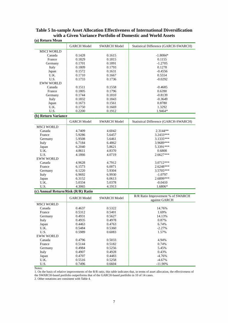
7

Table 5 In-sample Asset Allocation Effectiveness of International Diversificationwith a Given Variance Portfolio of Domestic and World Assets

(a) Return MeanGARCH Model SWARCH Model Statistical Difference (GARCH-SWARCH)

MSCI WORLDCanada 0.1428 0.1615 -1.8084*France 0.1829 0.1815 0.1155

Germany 0.1701 0.1891 -1.2705Italy 0.1809 0.1793 0.1278Japan 0.1572 0.1631 -0.4556U.K. 0.1710 0.1667 0.5554U.S. 0.1733 0.1736 -0.0292

EWW WORLDCanada 0.1511 0.1558 -0.4685France 0.1805 0.1796 0.6390

Germany 0.1744 0.1810 -0.8139Italy 0.1832 0.1843 -0.3649Japan 0.1673 0.1561 0.8780U.K. 0.1750 0.1669 1.3292U.S. 0.2200 0.1912 1.9464*

(b) Return VarianceGARCH Model SWARCH Model Statistical Difference (GARCH-SWARCH)

MSCI WORLDCanada 4.7409 4.6042 2.3144**France 5.9286 5.6457 3.2433***Germany 5.9508 5.6461 3.1335***Italy 6.7184 6.4862 3.9689***Japan 6.2040 5.8621 5.3391***U.K. 4.8611 4.8370 0.6808U.S. 4.1866 4.0719 2.6627***

EWW WORLDCanada 4.9628 4.7912 3.0712***France 6.1573 6.0071 2.6248***Germany 6.1220 5.9304 3.5705***Italy 6.9692 6.9930 -1.0797Japan 6.3152 6.0613 2.6899***U.K. 5.0334 5.0378 -0.0410U.S. 4.3065 4.1913 1.6806*

(c) Annual Return/Risk (R/R) Ratio

GARCH Model SWARCH Model R/R Ratio Improvement % of SWARCHagainst GARCH

MSCI WORLDCanada 0.4637 0.5322 14.76%France 0.5312 0.5401 1.69%Germany 0.4931 0.5627 14.13%Italy 0.4935 0.4978 0.87%Japan 0.4463 0.4763 6.74%U.K. 0.5484 0.5360 -2.27%U.S. 0.5989 0.6083 1.57%

EWW WORLDCanada 0.4796 0.5033 4.94%France 0.5144 0.5182 0.74%Germany 0.4984 0.5256 5.45%Italy 0.4907 0.4928 0.43%Japan 0.4707 0.4483 -4.76%U.K. 0.5516 0.5258 -4.67%U.S. 0.7496 0.6604 -11.90%

Notes:1. On the basis of relative improvements of the R/R ratio, this table indicates that, in terms of asset allocation, the effectiveness ofthe SWARCH-based portfolio outperforms that of the GARCH-based portfolio in 10 of 14 cases.2. Other notations are consistent with Table 4.

8

Table 6 Observation Percentages of Various Market StatesWhole Period World=LV and Indl.=LV World=HV and Indl=LV World=LV and Indl=HV World=HV and Indl=HV

MSCI-WORLDMSCI-Canada 100% 60.86%* 15.11% 13.00% 11.03%MSCI-France 100% 63.39%* 13.14% 13.91% 9.56%MSCI-Germany 100% 46.03%* 19.33% 13.63% 21.01%MSCI-Italy 100% 26.77% 11.04% 38.23%* 23.96%MSCI-Japan 100% 61.28%* 25.72% 3.30% 9.70%MSCI-U.K. 100% 33.66%* 11.67% 29.73% 24.94%MSCI-U.S. 100% 29.80% 19.47% 18.90% 31.83%*

EWW-WORLDEWW-Canada 100% 61.21%* 15.39% 12.86% 10.54%EWW-France 100% 36.05%* 10.19% 29.80% 23.96%EWW-Germany 100% 55.87%* 12.16% 16.16% 15.81%EWW-Italy 100% 12.37% 0.56% 61.49%* 25.58%EWW-Japan 100% 53.90%* 11.38% 24.46% 10.26%EWW-U.K. 100% 33.73% 8.85% 37.60%* 19.82%EWW-U.S. 100% 29.73% 5.06% 37.81%* 27.40%

Average 100% 43.19%* 12.79% 25.06% 18.96%Notes:1. To identify the specific volatility state existing at each point in time, the estimated filtering probability of a specific state (see Fig. 2 as an example) and a maximum value criterion are here used. In other words, attime t, if the estimated value of the filtering probability of the “HV-HV”state (st=4 or st

y =2 and stx =2) exceeds that of the three alternative states, then an “HV-HV”state is said to exist at this point in time. More

generally, this work defines the market as being in a specific state if the corresponding estimated state probability is relatively high.2. This table lists observation percentages of various volatility states. The * denotes the maximum value among the four state combinations, which is the “LV and LV” state in 9 of 14 cases. This finding is consistentwith the notion that a low volatility state is more persistent than a high volatility state. This claim is further validated by the fact that Table 3 indicates that the py

11 (px11) estimates generally exceed the py

22 (px22 )

estimates.

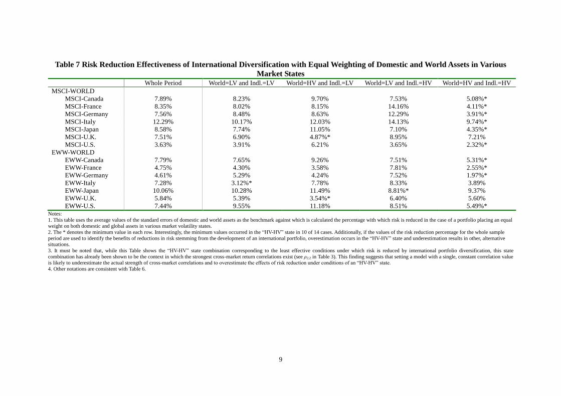
9

Table 7 Risk Reduction Effectiveness of International Diversification with Equal Weighting of Domestic and World Assets in VariousMarket States

Whole Period World=LV and Indl.=LV World=HV and Indl.=LV World=LV and Indl.=HV World=HV and Indl.=HVMSCI-WORLD

MSCI-Canada 7.89% 8.23% 9.70% 7.53% 5.08%*MSCI-France 8.35% 8.02% 8.15% 14.16% 4.11%*MSCI-Germany 7.56% 8.48% 8.63% 12.29% 3.91%*MSCI-Italy 12.29% 10.17% 12.03% 14.13% 9.74%*MSCI-Japan 8.58% 7.74% 11.05% 7.10% 4.35%*MSCI-U.K. 7.51% 6.90% 4.87%* 8.95% 7.21%MSCI-U.S. 3.63% 3.91% 6.21% 3.65% 2.32%*

EWW-WORLDEWW-Canada 7.79% 7.65% 9.26% 7.51% 5.31%*EWW-France 4.75% 4.30% 3.58% 7.81% 2.55%*EWW-Germany 4.61% 5.29% 4.24% 7.52% 1.97%*EWW-Italy 7.28% 3.12%* 7.78% 8.33% 3.89%EWW-Japan 10.06% 10.28% 11.49% 8.81%* 9.37%EWW-U.K. 5.84% 5.39% 3.54%* 6.40% 5.60%EWW-U.S. 7.44% 9.55% 11.18% 8.51% 5.49%*

Notes:1. This table uses the average values of the standard errors of domestic and world assets as the benchmark against which is calculated the percentage with which risk is reduced in the case of a portfolio placing an equalweight on both domestic and global assets in various market volatility states.2. The * denotes the minimum value in each row. Interestingly, the minimum values occurred in the“HV-HV”state in 10 of 14 cases. Additionally, if the values of the risk reduction percentage for the whole sampleperiod are used to identify the benefits of reductions in risk stemming from the development of an international portfolio, overestimation occurs in the “HV-HV”state and underestimation results in other, alternativesituations.3. It must be noted that, while this Table shows the “HV-HV”state combination corresponding to the least effective conditions under which risk is reduced by international portfolio diversification, this statecombination has already been shown to be the context in which the strongest cross-market return correlations exist (see ρ2,2 in Table 3). This finding suggests that setting a model with a single, constant correlation valueis likely to underestimate the actual strength of cross-market correlations and to overestimate the effects of risk reduction under conditions of an “HV-HV” state.4. Other notations are consistent with Table 6.

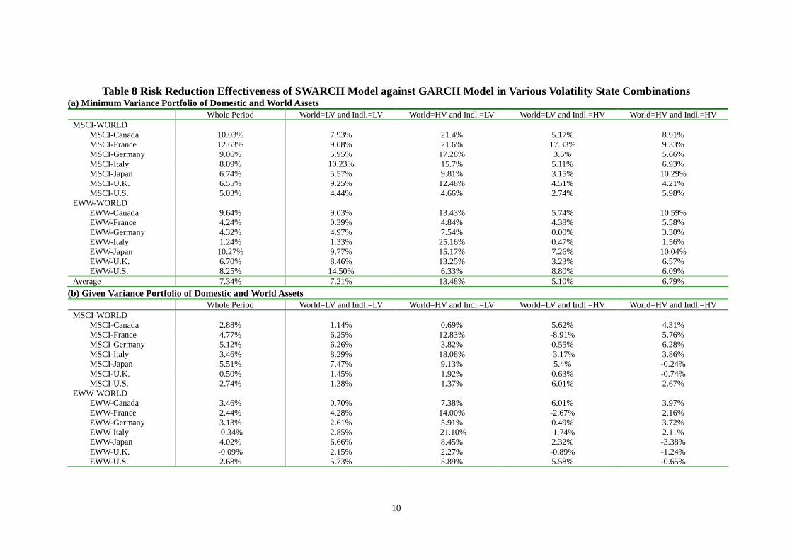
10

Table 8 Risk Reduction Effectiveness of SWARCH Model against GARCH Model in Various Volatility State Combinations(a) Minimum Variance Portfolio of Domestic and World Assets

Whole Period World=LV and Indl.=LV World=HV and Indl.=LV World=LV and Indl.=HV World=HV and Indl.=HVMSCI-WORLD

MSCI-Canada 10.03% 7.93% 21.4% 5.17% 8.91%MSCI-France 12.63% 9.08% 21.6% 17.33% 9.33%MSCI-Germany 9.06% 5.95% 17.28% 3.5% 5.66%MSCI-Italy 8.09% 10.23% 15.7% 5.11% 6.93%MSCI-Japan 6.74% 5.57% 9.81% 3.15% 10.29%MSCI-U.K. 6.55% 9.25% 12.48% 4.51% 4.21%MSCI-U.S. 5.03% 4.44% 4.66% 2.74% 5.98%

EWW-WORLDEWW-Canada 9.64% 9.03% 13.43% 5.74% 10.59%EWW-France 4.24% 0.39% 4.84% 4.38% 5.58%EWW-Germany 4.32% 4.97% 7.54% 0.00% 3.30%EWW-Italy 1.24% 1.33% 25.16% 0.47% 1.56%EWW-Japan 10.27% 9.77% 15.17% 7.26% 10.04%EWW-U.K. 6.70% 8.46% 13.25% 3.23% 6.57%EWW-U.S. 8.25% 14.50% 6.33% 8.80% 6.09%

Average 7.34% 7.21% 13.48% 5.10% 6.79%(b) Given Variance Portfolio of Domestic and World Assets

Whole Period World=LV and Indl.=LV World=HV and Indl.=LV World=LV and Indl.=HV World=HV and Indl.=HVMSCI-WORLD

MSCI-Canada 2.88% 1.14% 0.69% 5.62% 4.31%MSCI-France 4.77% 6.25% 12.83% -8.91% 5.76%MSCI-Germany 5.12% 6.26% 3.82% 0.55% 6.28%MSCI-Italy 3.46% 8.29% 18.08% -3.17% 3.86%MSCI-Japan 5.51% 7.47% 9.13% 5.4% -0.24%MSCI-U.K. 0.50% 1.45% 1.92% 0.63% -0.74%MSCI-U.S. 2.74% 1.38% 1.37% 6.01% 2.67%

EWW-WORLDEWW-Canada 3.46% 0.70% 7.38% 6.01% 3.97%EWW-France 2.44% 4.28% 14.00% -2.67% 2.16%EWW-Germany 3.13% 2.61% 5.91% 0.49% 3.72%EWW-Italy -0.34% 2.85% -21.10% -1.74% 2.11%EWW-Japan 4.02% 6.66% 8.45% 2.32% -3.38%EWW-U.K. -0.09% 2.15% 2.27% -0.89% -1.24%EWW-U.S. 2.68% 5.73% 5.89% 5.58% -0.65%

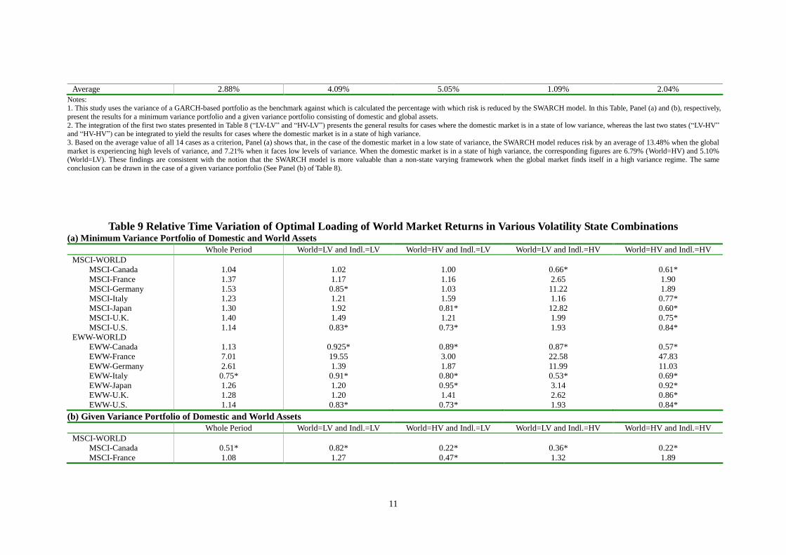
11

Average 2.88% 4.09% 5.05% 1.09% 2.04%Notes:1. This study uses the variance of a GARCH-based portfolio as the benchmark against which is calculated the percentage with which risk is reduced by the SWARCH model. In this Table, Panel (a) and (b), respectively,present the results for a minimum variance portfolio and a given variance portfolio consisting of domestic and global assets.2. The integration of the first two states presented in Table 8 (“LV-LV”and“HV-LV”) presents the general results for cases where the domestic market is in a state of low variance, whereas the last two states (“LV-HV”and“HV-HV”)can be integrated to yield the results for cases where the domestic market is in a state of high variance.3. Based on the average value of all 14 cases as a criterion, Panel (a) shows that, in the case of the domestic market in a low state of variance, the SWARCH model reduces risk by an average of 13.48% when the globalmarket is experiencing high levels of variance, and 7.21% when it faces low levels of variance. When the domestic market is in a state of high variance, the corresponding figures are 6.79% (World=HV) and 5.10%(World=LV). These findings are consistent with the notion that the SWARCH model is more valuable than a non-state varying framework when the global market finds itself in a high variance regime. The sameconclusion can be drawn in the case of a given variance portfolio (See Panel (b) of Table 8).

Table 9 Relative Time Variation of Optimal Loading of World Market Returns in Various Volatility State Combinations(a) Minimum Variance Portfolio of Domestic and World Assets

Whole Period World=LV and Indl.=LV World=HV and Indl.=LV World=LV and Indl.=HV World=HV and Indl.=HVMSCI-WORLD

MSCI-Canada 1.04 1.02 1.00 0.66* 0.61*MSCI-France 1.37 1.17 1.16 2.65 1.90MSCI-Germany 1.53 0.85* 1.03 11.22 1.89MSCI-Italy 1.23 1.21 1.59 1.16 0.77*MSCI-Japan 1.30 1.92 0.81* 12.82 0.60*MSCI-U.K. 1.40 1.49 1.21 1.99 0.75*MSCI-U.S. 1.14 0.83* 0.73* 1.93 0.84*

EWW-WORLDEWW-Canada 1.13 0.925* 0.89* 0.87* 0.57*EWW-France 7.01 19.55 3.00 22.58 47.83EWW-Germany 2.61 1.39 1.87 11.99 11.03EWW-Italy 0.75* 0.91* 0.80* 0.53* 0.69*EWW-Japan 1.26 1.20 0.95* 3.14 0.92*EWW-U.K. 1.28 1.20 1.41 2.62 0.86*EWW-U.S. 1.14 0.83* 0.73* 1.93 0.84*

(b) Given Variance Portfolio of Domestic and World AssetsWhole Period World=LV and Indl.=LV World=HV and Indl.=LV World=LV and Indl.=HV World=HV and Indl.=HV

MSCI-WORLDMSCI-Canada 0.51* 0.82* 0.22* 0.36* 0.22*MSCI-France 1.08 1.27 0.47* 1.32 1.89

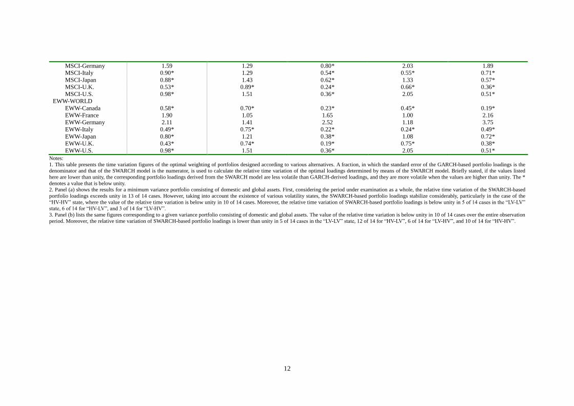
12

MSCI-Germany 1.59 1.29 0.80* 2.03 1.89MSCI-Italy 0.90* 1.29 0.54* 0.55* 0.71*MSCI-Japan 0.88* 1.43 0.62* 1.33 0.57*MSCI-U.K. 0.53* 0.89* 0.24* 0.66* 0.36*MSCI-U.S. 0.98* 1.51 0.36* 2.05 0.51*

EWW-WORLDEWW-Canada 0.58* 0.70* 0.23* 0.45* 0.19*EWW-France 1.90 1.05 1.65 1.00 2.16EWW-Germany 2.11 1.41 2.52 1.18 3.75EWW-Italy 0.49* 0.75* 0.22* 0.24* 0.49*EWW-Japan 0.80* 1.21 0.38* 1.08 0.72*EWW-U.K. 0.43* 0.74* 0.19* 0.75* 0.38*EWW-U.S. 0.98* 1.51 0.36* 2.05 0.51*

Notes:1. This table presents the time variation figures of the optimal weighting of portfolios designed according to various alternatives. A fraction, in which the standard error of the GARCH-based portfolio loadings is thedenominator and that of the SWARCH model is the numerator, is used to calculate the relative time variation of the optimal loadings determined by means of the SWARCH model. Briefly stated, if the values listedhere are lower than unity, the corresponding portfolio loadings derived from the SWARCH model are less volatile than GARCH-derived loadings, and they are more volatile when the values are higher than unity. The *denotes a value that is below unity.2. Panel (a) shows the results for a minimum variance portfolio consisting of domestic and global assets. First, considering the period under examination as a whole, the relative time variation of the SWARCH-basedportfolio loadings exceeds unity in 13 of 14 cases. However, taking into account the existence of various volatility states, the SWARCH-based portfolio loadings stabilize considerably, particularly in the case of the“HV-HV”state, where the value of the relative time variation is below unity in 10 of 14 cases. Moreover, the relative time variation of SWARCH-based portfolio loadings is below unityin 5 of 14 cases in the “LV-LV” state, 6 of 14 for “HV-LV”, and 3 of 14 for “LV-HV”.3. Panel (b) lists the same figures corresponding to a given variance portfolio consisting of domestic and global assets. The value of the relative time variation is below unity in 10 of 14 cases over the entire observationperiod. Moreover, the relative time variation of SWARCH-based portfolio loadings is lower than unity in 5 of 14 cases in the “LV-LV” state, 12 of 14 for“HV-LV”, 6 of 14 for “LV-HV”,and 10 of 14 for “HV-HV”.

13

Table 10 Out-of-Sample Asset Allocation Effectiveness of InternationalDiversification with a Minimum Variance Portfolio of Domestic and World

Assets(a) Return Mean

GARCH Model SWARCH Model Statistical Difference (GARCH-SWARCH)

MSCI WORLDMSCI-Japan 0.2928 0.2804 0.7842MSCI-U.K. 0.2871 0.2879 -0.0528MSCI-U.S. 0.2699 0.2652 0.8802

EWW WORLDEWW-Japan 0.3431 0.3455 -0.1779EWW-U.K. 0.3234 0.3140 0.8366EWW-U.S. 0.2705 0.2740 -0.4244

(b) Return VarianceGARCH Model SWARCH Model Statistical Difference (GARCH-SWARCH)

MSCI WORLDMSCI-Japan 1.9137 2.0784 -1.9526*MSCI-U.K. 1.6786 1.6898 -0.4813MSCI-U.S. 1.6670 1.6585 1.0273

EWW WORLDEWW-Japan 2.6954 2.8709 -2.2239**EWW-U.K. 2.6638 2.6971 -1.2240EWW-U.S. 1.8106 1.8260 -0.5809

(c) Annual Return/Risk (R/R) Ratio

GARCH Model SWARCH Model R/R Ratio Improvement % of SWARCHagainst GARCH

MSCI WORLDMSCI-Japan 1.4967 1.3751 -8.12%MSCI-U.K. 1.5667 1.5663 -0.03%MSCI-U.S. 1.4784 1.4563 -1.50%

EWW WORLDEWW-Japan 1.4777 1.4417 -2.43%EWW-U.K. 1.4013 1.3521 -3.51%EWW-U.S. 1.4213 1.4339 0.88%

Notes:1. In order to carry out rolling estimations in the context of out-of-sample testing, the last 200 weekly observations of the sample(or nearly four years’ worth ofdata) are withdrawn to make up the inputs in this process.2. Following the addition of each subsequent observation, the sample is rolled; that is, the deliberate deletion of the oldestobservation coincides with the addition of the most recent one. This technique thus fixes the sample size at 1,226 (= 1,426 - 200)observations. In this case, as in that of the in-sample test, the SWARCH and GARCH models are compared in terms of theirrespective effectiveness in allocating assets.3. With the SWARCH model, the out-of-sample predicted portfolio loadings at time t+1 are obtained according to a two-stepprocedure. First, the estimated population parameters at time t are employed to forecast the regime probabilities at time t+1.Second, the one-step-ahead forecasts thus derived are used to determine the loadings of the corresponding state-varying portfolioat time t+1.4. To facilitate the process of convergence, the estimate for each individual period calculated in the non-linear estimation processis used as the initial value in the calculation of the estimate for the period immediately following it.5. The ***, ** and * denote the 1%, 2.5% and 5% levels of significance, respectively. See the appendix for details of thestatistical test of whether the variances of portfolio returns vary significantly between the bivariate GARCH and SWARCHmodels.6. In the case of the minimum variance portfolio tested here, the SWARCH model underperforms the GARCH model in mostcases. More specifically, the variance of a SWARCH-based portfolio exceeds that for the GARCH model in 5 of 6 cases, and itdoes so significantly in two instances. Moreover, the annual R/R ratio calculated for the SWARCH-based portfolio is lower thanthat obtained in the case of the GARCH model in 5 of 6 cases.

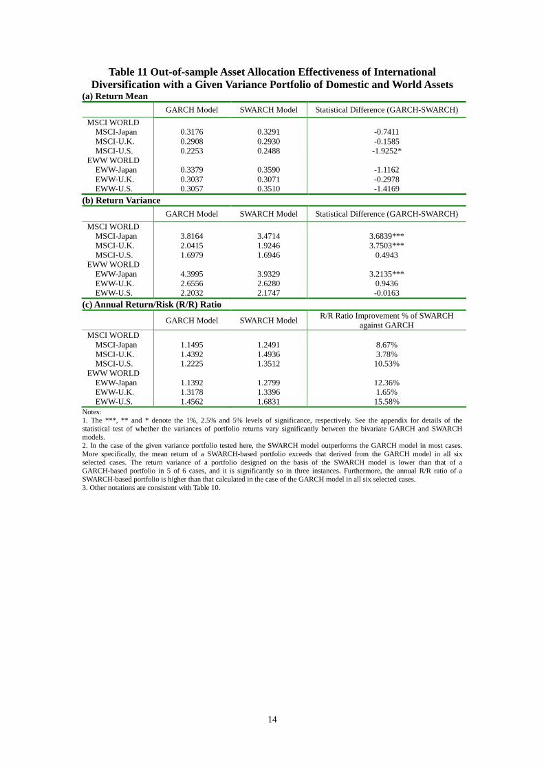
14

Table 11 Out-of-sample Asset Allocation Effectiveness of InternationalDiversification with a Given Variance Portfolio of Domestic and World Assets

(a) Return MeanGARCH Model SWARCH Model Statistical Difference (GARCH-SWARCH)

MSCI WORLDMSCI-Japan 0.3176 0.3291 -0.7411MSCI-U.K. 0.2908 0.2930 -0.1585MSCI-U.S. 0.2253 0.2488 -1.9252*

EWW WORLDEWW-Japan 0.3379 0.3590 -1.1162EWW-U.K. 0.3037 0.3071 -0.2978EWW-U.S. 0.3057 0.3510 -1.4169

(b) Return VarianceGARCH Model SWARCH Model Statistical Difference (GARCH-SWARCH)

MSCI WORLDMSCI-Japan 3.8164 3.4714 3.6839***MSCI-U.K. 2.0415 1.9246 3.7503***MSCI-U.S. 1.6979 1.6946 0.4943

EWW WORLDEWW-Japan 4.3995 3.9329 3.2135***EWW-U.K. 2.6556 2.6280 0.9436EWW-U.S. 2.2032 2.1747 -0.0163

(c) Annual Return/Risk (R/R) Ratio

GARCH Model SWARCH Model R/R Ratio Improvement % of SWARCHagainst GARCH

MSCI WORLDMSCI-Japan 1.1495 1.2491 8.67%MSCI-U.K. 1.4392 1.4936 3.78%MSCI-U.S. 1.2225 1.3512 10.53%

EWW WORLDEWW-Japan 1.1392 1.2799 12.36%EWW-U.K. 1.3178 1.3396 1.65%EWW-U.S. 1.4562 1.6831 15.58%

Notes:1. The ***, ** and * denote the 1%, 2.5% and 5% levels of significance, respectively. See the appendix for details of thestatistical test of whether the variances of portfolio returns vary significantly between the bivariate GARCH and SWARCHmodels.2. In the case of the given variance portfolio tested here, the SWARCH model outperforms the GARCH model in most cases.More specifically, the mean return of a SWARCH-based portfolio exceeds that derived from the GARCH model in all sixselected cases. The return variance of a portfolio designed on the basis of the SWARCH model is lower than that of aGARCH-based portfolio in 5 of 6 cases, and it is significantly so in three instances. Furthermore, the annual R/R ratio of aSWARCH-based portfolio is higher than that calculated in the case of the GARCH model in all six selected cases.3. Other notations are consistent with Table 10.

(a) MSCI World Index

-20

-15

-10

-5

0

5

10

15

1980/1 1983/1 1986/1 1989/1 1992/1 1995/1 1998/1 2001/1 2004/1 2007/1

(b) U.S. Stock Market Index

-20

-15

-10

-5

0

5

10

15

1980/1 1983/1 1986/1 1989/1 1992/1 1995/1 1998/1 2001/1 2004/1 2007/1

Table 1 Global and Domestic Market Returns: The Case of MSCI-U.S.

(a) World=LV and Indl.=LV (b) World=HV and Indl.=LV

0

0.25

0.5

0.75

1

1980/1 1983/1 1986/1 1989/1 1992/1 1995/1 1998/1 2001/1 2004/1 2007/10

0.25

0.5

0.75

1

1980/1 1983/1 1986/1 1989/1 1992/1 1995/1 1998/1 2001/1 2004/1 2007/1

(c) World=LV and Indl.=HV (d) World=HV and Indl.=HV

0

0.25

0.5

0.75

1

1980/1 1983/1 1986/1 1989/1 1992/1 1995/1 1998/1 2001/1 2004/1 2007/10

0.25

0.5

0.75

1

1980/1 1983/1 1986/1 1989/1 1992/1 1995/1 1998/1 2001/1 2004/1 2007/1

Figure 2 SWARCH-based Estimates of the Filtering Probabilities of Specific Volatility State Combinations for the Illustrative Case ofMSCI-U.S.

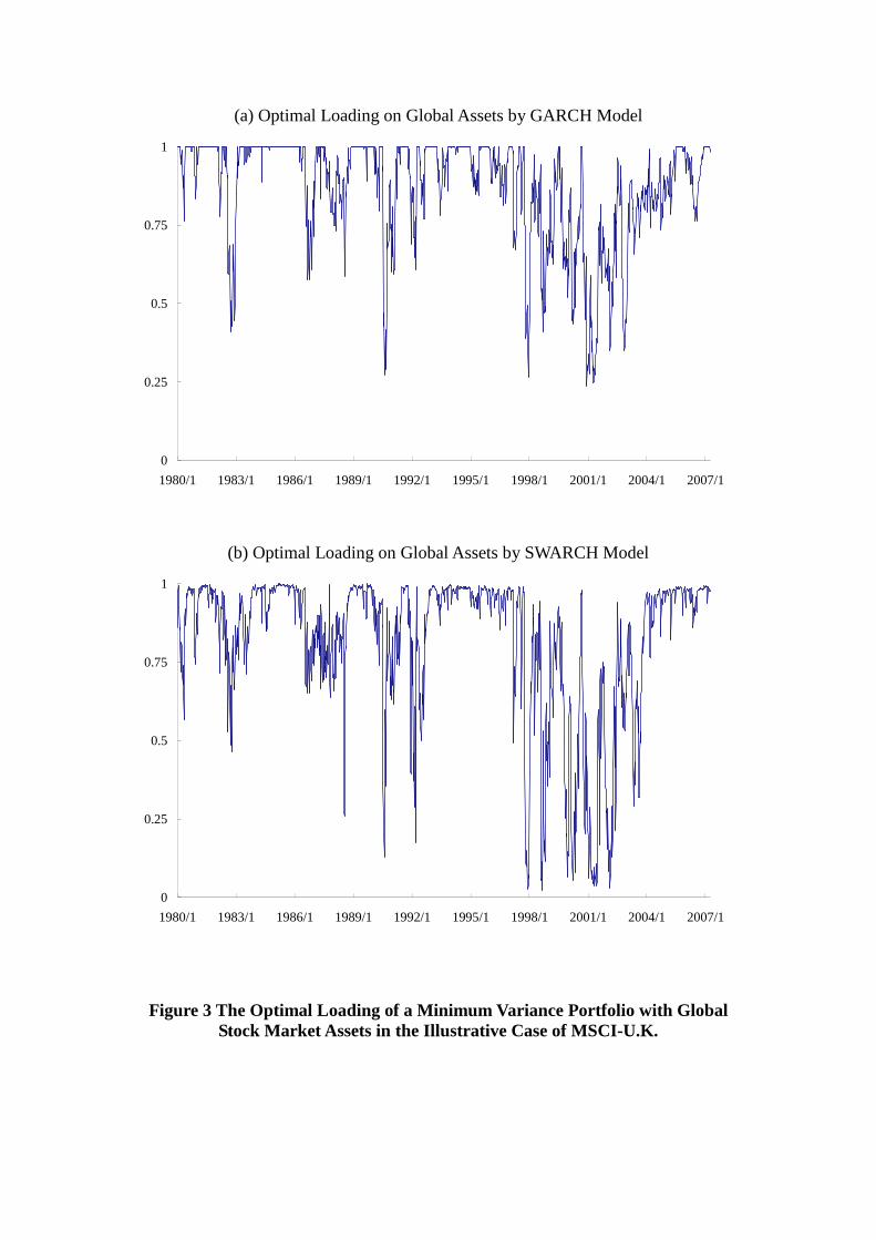
(a) Optimal Loading on Global Assets by GARCH Model

0

0.25

0.5

0.75

1

1980/1 1983/1 1986/1 1989/1 1992/1 1995/1 1998/1 2001/1 2004/1 2007/1

(b) Optimal Loading on Global Assets by SWARCH Model

0

0.25

0.5

0.75

1

1980/1 1983/1 1986/1 1989/1 1992/1 1995/1 1998/1 2001/1 2004/1 2007/1

Figure 3 The Optimal Loading of a Minimum Variance Portfolio with GlobalStock Market Assets in the Illustrative Case of MSCI-U.K.

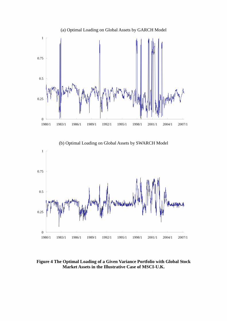
(a) Optimal Loading on Global Assets by GARCH Model

0

0.25

0.5

0.75

1

1980/1 1983/1 1986/1 1989/1 1992/1 1995/1 1998/1 2001/1 2004/1 2007/1

(b) Optimal Loading on Global Assets by SWARCH Model

0

0.25

0.5

0.75

1

1980/1 1983/1 1986/1 1989/1 1992/1 1995/1 1998/1 2001/1 2004/1 2007/1

Figure 4 The Optimal Loading of a Given Variance Portfolio with Global StockMarket Assets in the Illustrative Case of MSCI-U.K.

(a) World=LV and Indl.=LV (b) World=HV and Indl.=LV

0

0.25

0.5

0.75

1

2003/7 2004/1 2004/7 2005/1 2005/7 2006/1 2006/7 2007/10

0.25

0.5

0.75

1

2003/7 2004/1 2004/7 2005/1 2005/7 2006/1 2006/7 2007/1

(c) World=LV and Indl.=HV (d) World=HV and Indl.=HV

0

0.25

0.5

0.75

1

2003/7 2004/1 2004/7 2005/1 2005/7 2006/1 2006/7 2007/10

0.25

0.5

0.75

2003/7 2004/1 2004/7 2005/1 2005/7 2006/1 2006/7 2007/1

Figure 5 Rolling Regime Probability Forecasts Derived on the Basis of the SWARCH Model in the Illustrative Case of MSCI-Japan

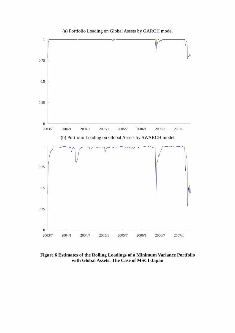
(a) Portfolio Loading on Global Assets by GARCH model

0

0.25

0.5

0.75

1

2003/7 2004/1 2004/7 2005/1 2005/7 2006/1 2006/7 2007/1

(b) Portfolio Loading on Global Assets by SWARCH model

0

0.25

0.5

0.75

1

2003/7 2004/1 2004/7 2005/1 2005/7 2006/1 2006/7 2007/1

Figure 6 Estimates of the Rolling Loadings of a Minimum Variance Portfoliowith Global Assets: The Case of MSCI-Japan

(a) Portfolio Loading on Global Assets by GARCH model

0

0.25

0.5

0.75

1

2003/7 2004/1 2004/7 2005/1 2005/7 2006/1 2006/7 2007/1

(b) Portfolio Loading on Global Assets by SWARCH model

0

0.25

0.5

0.75

1

2003/7 2004/1 2004/7 2005/1 2005/7 2006/1 2006/7 2007/1

Figure 7 Estimates of the Rolling Loadings of a Given Variance Portfolio withGlobal Assets: The Case of MSCI-Japan