voltage security margin assessment · voltage security margin assessment ... the industry advisors...

Voltage Security Margin Assessment

Final Project Report

Power Systems Engineering Research Center

A National Science FoundationIndustry/University Cooperative Research Center

since 1996

PSERC

Power Systems Engineering Research Center

Voltage Security Margin Assessment

Final Project Report

Project Team

Garng M. Huang Ali Abur

Texas A&M University

PSERC Publication 02-49

December 2002

Information about this Project For information about this project contact: Garng M. Huang Professor Electrical Engineering Department Texas A&M University College Station, TX 77840 Phone: 979-845-7476 Email: [email protected] Power Systems Engineering Research Center This is a project report from the Power Systems Engineering Research Center (PSERC). PSERC is a multi-university Center conducting research on challenges facing a restructuring electric power industry and educating the next generation of power engineers. More information about PSERC can be found at the Center’s website: http://www.pserc.wisc.edu. For additional information, contact: Power Systems Engineering Research Center Cornell University 428 Phillips Hall Ithaca, New York 14853 Phone: 607-255-5601 Fax: 607-255-8871 Notice Concerning Copyright Material PSERC members are given permission to copy without fee all or part of this publication for internal use if appropriate attribution is given to this document as the source material. This report is available for downloading from the PSERC website.

2002 Texas A&M University. All rights reserved.

http://www.pserc.wisc.edu/

i

ACKNOWLEDGEMENTS

The work described in this report was sponsored by the Power Systems Engineering Research Center (PSERC). We express our appreciation for the support provided by PSERC’s industrial members and by the National Science Foundation under grant NSF EEC-0002917 received under the Industry / University Cooperative Research Center program. The industry advisors for the project were Mani Subramanian, ABB Network Management; Don Sevcik, CenterPoint Energy; and Bruce Dietzman, Oncor. Their suggestions and contributions to the work are appreciated.

ii

EXECUTIVE SUMMARY Increasingly, within restructured power systems, voltage stability issues are becoming significant in the way we plan, operate and maintain the system. The involvement of new players in the electricity power business has led to the proliferation of intra-area and inter-area transactions of electricity in the transmission network. Typically, these transactions are of considerably shorter duration and larger variety than that in a vertically-integrated utility (VIU) structure where a single utility controls power generation, transmission and distribution within a given area. Not only does this new operating environment lead to frequent and significant changes in system operating points and load flow patterns, but it also results in increasing volatility in system conditions. This leads to potential security and reliability degradation in system operations, such as in voltage stability. There is a need to evolve procedures that insure voltage stability in the operation of more open and diverse power systems. To achieve this aim, power system operators need to be able to quickly assess from measurable quantities, the operational state of the system from the voltage stability perspective. At the same time, in case of stability problems, the responsibility evaluation procedures need to be distinctly identified within the new operating environment. The objective of this project was to evolve a framework, within the context of the restructured power market operations, to incorporate voltage stability assessment into the power system security, accountability and utilization factors for control devices. In the course of completing the objective of this project, we have come up with new and practical algorithms and procedures that can effectively address the incorporation of voltage stability into market-oriented power system operations. We summarize the significant outcomes of our work as given below. Dynamic modeling of generators, governors, ULTC, switched capacitor and loads

using EUROSTAG has been carried to study dynamic voltage stability and the importance of dynamic reserves to maintain stability [8]. Detecting dynamic voltage collapse using state information has been investigated for a variety of dynamic disturbances [4]. Static modeling of FACTS devices in investigating voltage stability studies also has been carried out. It is observed that usage of devices such as TCSC and SVC could improve stability margin significantly [3].

A new way of using bifurcation analysis, using the unreduced Jacobian matrix [7] that

avoids singularity induced infinity problem and is computationally attractive, has been formulated.

Within the context of an open power market, the responsibility evaluation of a

potential voltage collapse assumes significance. Using bifurcation analysis, a procedure to allocate contribution of generators, transmission and control elements in voltage stability has been evolved [6]. This could be used as the basis for evaluating the utilization factors and the pricing of control elements in a power system.

iii

An algorithm to compute Optimal Power Flow incorporating voltage stability has

been proposed [1]. The voltage stability constraint is computed from the power flow state variables and the network topology. This algorithm has been applied further to evaluate reliability indices in planning stages [2]. The incorporation of voltage stability enhancement devices (such as FACTS devices) into the algorithm has also been formulated [3].

The framework for transaction-based power flow analysis for transmission utilization

allocation has been proposed [10]. The methods to model transactions for both pool type and point-to-point long-term bilateral type transaction have been designed. This analysis has been used to address the approach to equitable loss allocation in a competitive market [11]. The approach has been applied to congestion management and responsibility evaluation in such a market [9].

A new way to evaluate voltage stability responsibility in a composite market model

framework, having both the pool type spot market and the bilateral long-term transactions, has been devised [5]. This decomposition approach has the potential to address voltage stability usage, voltage security pricing and responsibility settlement in a transaction-based power market.

iv

TABLE OF CONTENTS

1 Voltage Stability Studies and Modeling Issues............................................................... 1 1.1 Typical two-bus system for voltage stability studies................................................. 1

1.1.1 Test system used for simulation .......................................................................... 2 1.1.2 Effects studied ..................................................................................................... 2 1.1.3 Software used for simulation............................................................................... 3

1.2 Power factor issues on static voltage collapse limits ................................................. 3 1.3 Modeling of TCSC and its effect on static voltage stability analysis ........................ 3 1.4 Modeling of SVC and its effect on voltage stability analysis.................................... 4 1.5 Modeling of load and its effect on voltage stability margins..................................... 7 1.6 Summary of observations for the two-bus case study ............................................... 9

2 Stability Index for Static Voltage Security Analysis .................................................... 10 2.1 Voltage collapse point at load bus using a two-bus model...................................... 10

2.1.1 Formulate a stability indicator........................................................................... 11 2.1.2 Numerical verification....................................................................................... 13 2.1.3 Index L with TCSC for scenario given in section 1.3 ....................................... 14

2.2 Extension of the two-bus voltage stability index L theory to a multi-bus system... 15 2.2.1 Multi-bus test system......................................................................................... 17 2.2.2 Case scenarios presented ................................................................................... 17

2.3 Results for the cases................................................................................................. 18 2.3.1 Case I(a): Increasing load at bus 5 and observing the index L.......................... 18 2.3.2 Case I(b): Effect of index L, at distant load bus, with increased loading at local load bus .......................................................................................................... 19 2.3.3 Case I(c): Effect of index L, at adjacent bus without load, with increased loading at local load bus ............................................................................................. 20 2.3.4 Case II: Increasing load at bus 7 and observing the index L............................. 21 2.3.5 Case III: Increasing load at bus 9 and observing the index L............................ 22 2.3.6 Summary for the multi-bus scenarios................................................................ 22

3 Dynamic Voltage Stability Issues ................................................................................. 23 3.1 Applying index L to dynamic voltage stability studies ........................................... 23 3.2 Objective 1: Interaction of remote buses and local buses........................................ 23 3.3 Objective 2: L as a dynamic stability indicator ....................................................... 24 3.4 Objective 3: L as an overall system profile indicator .............................................. 26 3.5 Objective 4: L as stability indicator for loss of a line .............................................. 30

3.5.1 Graphical plots for objective 4: L as stability indicator for loss of a line ......... 33 3.5.2 Observations for objective 4: L as stability indicator for loss of a line............. 34

3.6 Objective 5: Impacts of Z on L as an indicator........................................................ 35 3.7 Publications.............................................................................................................. 37

4 Voltage Stability Constrained OPF Algorithm ............................................................. 38 4.1 Algorithm................................................................................................................. 38 4.2 An illustration .......................................................................................................... 39 4.3 Observations ............................................................................................................ 40 4.4 Publications.............................................................................................................. 40

v

TABLE OF CONTENTS (continued) 5 Transaction-Based Stability Margin and Utilization Factors Evaluation...................... 41

5.1 Theory behind transaction-based power flow.......................................................... 41 5.2 Transaction-based power flow algorithm ................................................................ 43

5.2.1 Assumptions ...................................................................................................... 43 5.2.2 Step-wise procedures for decomposition........................................................... 43

5.3 Transaction-based voltage security margin allocation algorithm ............................ 48 5.3.1 Test case for demonstrating the voltage security margin allocation algorithm.51 5.3.2 Results for various scenarios ............................................................................. 53

5.4 Publications.............................................................................................................. 57 6 Bifurcation Analysis for Voltage Stability Margin Evaluation..................................... 59

6.1 Introduction.............................................................................................................. 60 6.1.1 Algebraic equations of load flow [6] .................................................................. 60 6.1.2 Differential equations of controllers.................................................................. 61

6.2 Dynamic stability margin vs. static stability margin ............................................... 62 6.3 Allocate the responsibility for voltage collapse with bifurcation analysis .............. 63

6.3.1 On P-regulator ................................................................................................... 64 6.3.2 On PI- regulator ................................................................................................. 66 6.3.3 On PID-regulator ............................................................................................... 68

6.5 The influence of the load pattern on the bifurcation points ..................................... 71 6.5.1 The influence of 0β ........................................................................................... 72 6.5.2 The influence of PE and QE on Pmax............................................................... 72 6.5.3 The influence of PE and QE on bifurcation points ........................................... 74

6.5.3.1 The influence of PE and QE on singular point C........................................ 74 6.5.3.2 The influence of PE and QE on other bifurcation points............................ 77

6.6 Publications.............................................................................................................. 77 7 Conclusions ................................................................................................................... 78 References ......................................................................................................................... 79

1

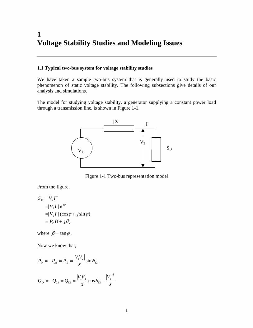
1 Voltage Stability Studies and Modeling Issues 1.1 Typical two-bus system for voltage stability studies We have taken a sample two-bus system that is generally used to study the basic phenomenon of static voltage stability. The following subsections give details of our analysis and simulations. The model for studying voltage stability, a generator supplying a constant power load through a transmission line, is shown in Figure 1-1.

Figure 1-1 Two-bus representation model

From the figure,

)1( )sin(cos||

||

2

2

*2

βφφ

φ

jPjIV

eIV

IVS

D

jD

+=+=

=

=

where φβ tan= . Now we know that,

1221

1221 sinθXVV

PPPD ==−=

XV

XVV

QQQD

21

1221

1221 cos −==−= θ

V1 SD

jX I

V2

Eliminating θ12 and solving the second order equation we finally get,

21

21

41

212

2 )(42

+−+−= VXPXP

VXP

VV DDD ββ (1.1)

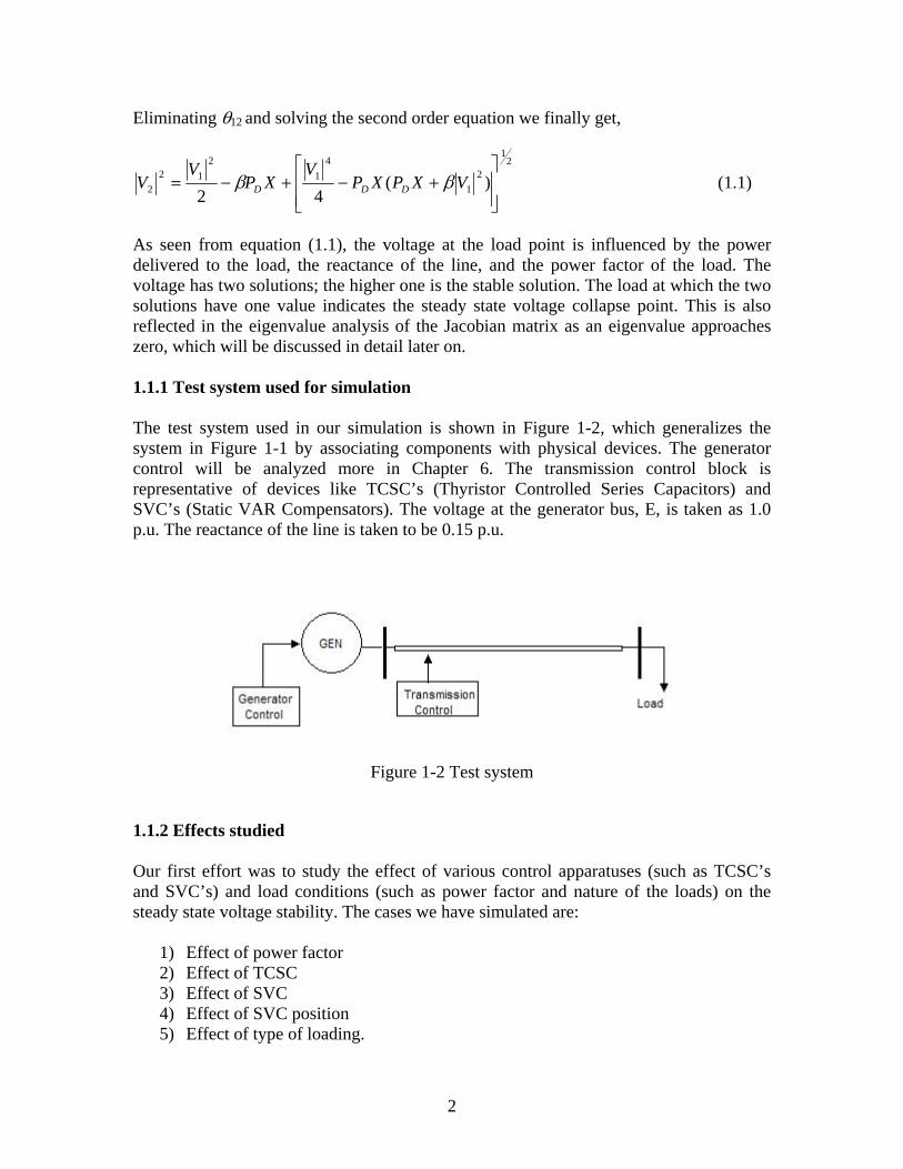
As seen from equation (1.1), the voltage at the load point is influenced by the power delivered to the load, the reactance of the line, and the power factor of the load. The voltage has two solutions; the higher one is the stable solution. The load at which the two solutions have one value indicates the steady state voltage collapse point. This is also reflected in the eigenvalue analysis of the Jacobian matrix as an eigenvalue approaches zero, which will be discussed in detail later on. 1.1.1 Test system used for simulation The test system used in our simulation is shown in Figure 1-2, which generalizes the system in Figure 1-1 by associating components with physical devices. The generator control will be analyzed more in Chapter 6. The transmission control block is representative of devices like TCSC’s (Thyristor Controlled Series Capacitors) and SVC’s (Static VAR Compensators). The voltage at the generator bus, E, is taken as 1.0 p.u. The reactance of the line is taken to be 0.15 p.u.

1.1.2 Effects studied Our first effort was to studyand SVC’s) and load conditisteady state voltage stability.

1) Effect of power factor2) Effect of TCSC 3) Effect of SVC 4) Effect of SVC positio5) Effect of type of loadi

2

Figure 1-2 Test system

the effect of various control apparatusons (such as power factor and nature The cases we have simulated are:

n ng.

es (such as TCSC’s of the loads) on the

3

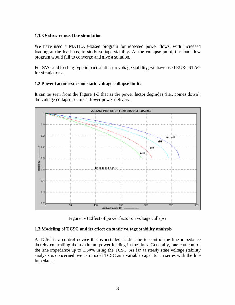
1.1.3 Software used for simulation We have used a MATLAB-based program for repeated power flows, with increased loading at the load bus, to study voltage stability. At the collapse point, the load flow program would fail to converge and give a solution. For SVC and loading-type impact studies on voltage stability, we have used EUROSTAG for simulations. 1.2 Power factor issues on static voltage collapse limits It can be seen from the Figure 1-3 that as the power factor degrades (i.e., comes down), the voltage collapse occurs at lower power delivery.

Figure 1-3 Effect of power factor on voltage collapse 1.3 Modeling of TCSC and its effect on static voltage stability analysis A TCSC is a control device that is installed in the line to control the line impedance thereby controlling the maximum power loading in the lines. Generally, one can control the line impedance up to ± 50% using the TCSC. As far as steady state voltage stability analysis is concerned, we can model TCSC as a variable capacitor in series with the line impedance.

4

Figure 1-4 Effect of TCSC on voltage stability It can be seen in Figure 1-4 that the lower the line impedance, the higher the voltage collapse point. Hence, it can be inferred that by employing TCSC’s to reduce line impedance for long lines, one can increase the voltage stability margin at the load end of the lines. 1.4 Modeling of SVC and its effect on voltage stability analysis SVC’s provides voltage support to the line. A SVC is modeled as a PV bus with zero real power in the power flow analysis. It is observed from Figure 1-5 that by employing a SVC at the middle of the line (i.e., supporting voltage in between the generation and load buses), one can improve the voltage stability margin at the load end. Moreover, by placing two SVC’s at equal distance between the buses, the collapse point increases further as shown in Figure 1-6.

5

Figure 1-5 Effect of SVC on voltage stability. Top curve represents voltage with a SVC at the middle of the transmission line. The bottom curve gives the voltage profile without a SVC.

Figure 1-6 Effect of number of SVC on voltage stability. Top curve is when there are two SVC’s and the middle curve is when there is one SVC at the middle of the line. For the bottom curve, there is no SVC.

6

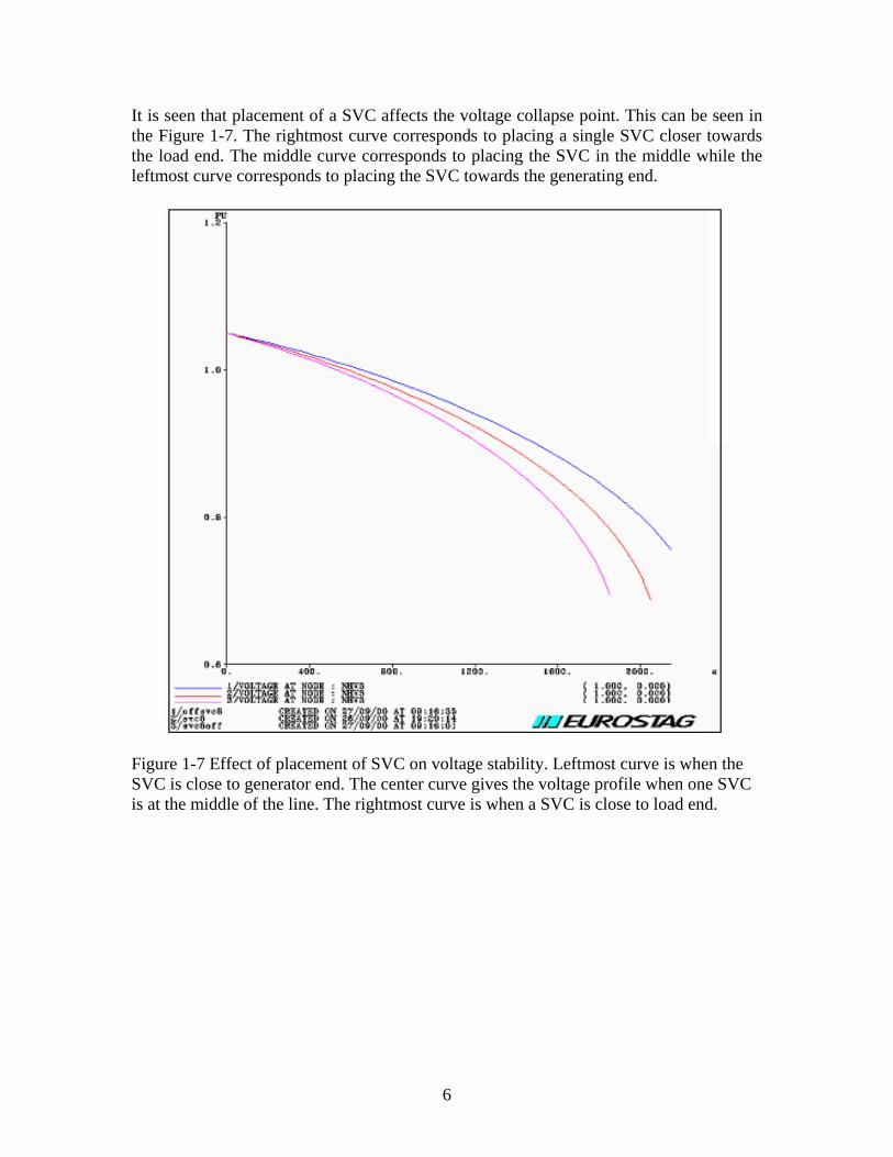
It is seen that placement of a SVC affects the voltage collapse point. This can be seen in the Figure 1-7. The rightmost curve corresponds to placing a single SVC closer towards the load end. The middle curve corresponds to placing the SVC in the middle while the leftmost curve corresponds to placing the SVC towards the generating end.

Figure 1-7 Effect of placement of SVC on voltage stability. Leftmost curve is when the SVC is close to generator end. The center curve gives the voltage profile when one SVC is at the middle of the line. The rightmost curve is when a SVC is close to load end.

7

1.5 Modeling of load and its effect on voltage stability margins The load modeling equation has been taken from the textbook by Carson Taylor on voltage stability [13], and is given by the following expression:

QfQv

PfPv

UUqQ

UUPP

=

=

000

000

ωω

ωω

We have chosen three types of load where the coefficients are given as follows:

Lighting: Pv = 1.54, Pf = 0.0, Qv = Qf = 0.0, P.F. = 1.0

Central A/C: Pv = 0.2, P f= 0.9, Qv = 2.2, Qf = -2.7, P.F. = 0.81

Refrigerator: Pv = 0.8, Pf = 0.5, Qv = 2.5, Qf = -1.4, P.F. = 0.84 To get the following curves, the load was increased in all the three cases starting from 1MW. The voltage profile with respect to increased loading is shown in Figure 1-8.

Figure 1-8 Effect of load type on voltage stability. Leftmost curve is for central A/C, middle curve for refrigeration, and rightmost curve for incandescent lighting.

8

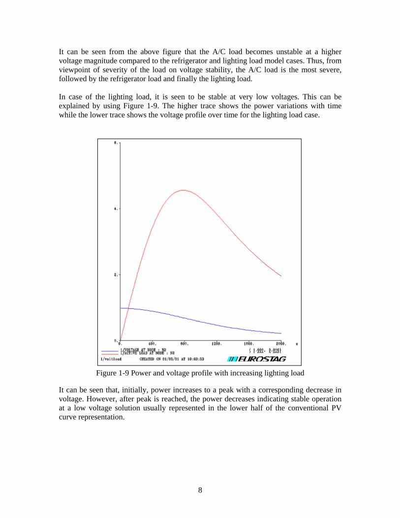
It can be seen from the above figure that the A/C load becomes unstable at a higher voltage magnitude compared to the refrigerator and lighting load model cases. Thus, from viewpoint of severity of the load on voltage stability, the A/C load is the most severe, followed by the refrigerator load and finally the lighting load. In case of the lighting load, it is seen to be stable at very low voltages. This can be explained by using Figure 1-9. The higher trace shows the power variations with time while the lower trace shows the voltage profile over time for the lighting load case.

Figure 1-9 Power and voltage profile with increasing lighting load

It can be seen that, initially, power increases to a peak with a corresponding decrease in voltage. However, after peak is reached, the power decreases indicating stable operation at a low voltage solution usually represented in the lower half of the conventional PV curve representation.

9

1.6 Summary of observations for the two-bus case study After running the simulations and observing the voltage collapse profiles, the following points became evident to us. 1) As X increases (longer lines), the collapse point lowers. This implies that the

likelihood of voltage collapse is more in the case of loads supplied from generation over a long distance.

2) Lower power factor impedance loads causes voltage collapse at lower power levels.

Hence, the limit of voltage stability margin for load buses operating at low power factors is less than load buses operating at high power factors.

3) It is very clearly seen from our simulations that the use of SVC’s improves stability

margin (i.e., the loading at which collapse point occurs). However, it is also seen that employing SVC’s very near to the load improves voltage stability margin more than when it is employed farther from the load bus.

4) The effect of load type on voltage stability was brought out distinctly in our

simulations. It can be seen from the simulation that voltage and frequency dependent loads (such as air conditioners and refrigerators) affect voltage collapse significantly.

10

2 Stability Index for Static Voltage Security Analysis 2.1 Voltage collapse point at load bus using a two-bus model

••

GG IS ,

Figure 2-1 Single generator and single load system

The simple system in Figure 2-1 has a load bus and a generator bus. We are interested in their voltage behavior. Using the nomenclature that a dot(.) on top of a variable indicates that it is a vector and a star(*) indicates it is the conjugate of that vector, we have:

D

DLGDQDD

V

SYVVYVI ∗

∗••••••

=−+= )( (2.1)

11011222

•∗••••∗••∗+=−+= YVVYVYVVYVYVS DDLGDLDQDD (2.2)

Here G

QL

LLQ V

YY

YVandYYY•

••

•••••

+−=+= 011 (2.3)

Since we would like to find the effect of load on the voltage, we would like to find

solution of DV•

. We represent the magnitude of DV•

as DV in the equation (2.2).

Let jbaY

S D +=•

∗

11

. Then, equation (2.2) is expressed as follows:

)sin()cos( 00002

02

11

DDDDDDDD VjVVVVVVVjba

Y

S δδδδ −+−+=+=+=∗•

•

∗

(2.4)

•

LY•

GV•

QY•

QYG DVLoad

11

D

DD VV

Va

0

2

0 )cos(cos −=−= δδδ (2.5)

DD VV

b

00 )sin(sin =−= δδδ (2.6)

Summing up, after squaring equations (2.5) and (2.6), would lead to the following.

2422222220 2)( bVaVabVaVV DDDD ++−=+−= (2.7)

Solving the equation (2.7) we get the following:

)1(42

2

11

220

40

20 −±=−+±+= rr

YS

baVV

aV

V DD (2.8)

because jbaY

S D +=•

∗

11

, hence )sin(),cos(1111

1111YS

DYS

DDD Y

Sb

YS

a φφφφ +−=+= . Then

)()2

(2

2222

02

0 baaV

aV

VD +−+±+=

112

22

11

20

11

20 )cos(

2)cos(

2 1111 YS

YSV

YSV D

YSD

YSD

DD−

++±++= φφφφ

)1( 2

11

−±= rrYSD (2.9)

Here r is defined as )cos(2 11

112

0YS

DDS

YVr φφ ++= (2.10)

2.1.1 Formulate a stability indicator

We can see that when 04

220

40 =−+ baV

V, the voltage at the node bus will collapse.

Now for G

QL

L VYY

YV•

••

••

+−=0 ;

12

when 04

220

40 ≥−+ baV

V, the voltage at node bus will be sustained; when

04

220

40 <−+ baV

V, the voltage cannot be sustained.

That is to say, the voltage collapse threshold is expressed 4

20

20

2 VVba −= .

Since jbaY

S D +=•

∗

11

, we can deduce the active power DP and reactive power DQ of

DS•

(where DDD jQPS +=•

) as follows:

))(Im()),(Re( 1111 jbaYQjbaYP DD +=+=••

We can get the corresponding curve in DS•

complex plane. Now, we can take this curve as the boundary of voltage collapse at the load node. This will help us formulate an indicator to reflect the proximity to this borderline. [14]

From equation (2.9), the voltage collapses when 1=r , 111

21 =YV

S

D

.

From the equation of (2.2), we can get:

DD V

V

YV

S•

•

•

∗

+= 0

112

1 1 (2.11)

So, we define an indicator L for voltage collapse as:

1121

112

101YV

S

YV

S

V

VLD

DD

==+= •

∗

•

•∆

(2.12)

When the load is zero ( 01 =•S ), then L=0; if the voltage at bus 1 collapses, L=1.

Let us consider this problem from the viewpoint of Jacobian matrix singularity. If the voltage at the load bus collapses, then the Jacobian matrix will be singular; that is, the determinant of the matrix will equal to zero. From equation (2.5) and (2.6), we can list the power flow equations for the above two-bus system as shown below:

aVVVVf DDD =+= 20 cos),( δδ

13

bVVVg DD == δδ sin),( 0

So, the corresponding Jacobian matrix is as follows:

−+=

δδδδ

cossinsincos2

00

00

VVVVVVV

JD

DD (2.13)

When the determinant of matrix J equals to zero, the voltage at the load bus will collapse:

21Recos0cos2)det(

00

200

2 −=

=⇒=+= •

•

V

VV

VVVVVJ DDDD

δδ

Then we can represent jbV

V D +−=•

•

21

0

where b is a real number, leading to:

1

21

21

21

111 0 =+−

+=

+−+=+ •

•

jb

jb

jbV

V

D

(2.14)

Actually, when we divide equation (2.2) by 112

•YVD , we get:

DD V

V

YV

S•

•

•

∗

+= 0

112

1 1 (2.15)

From the above analysis, we confirm that the indicator of voltage stability at load bus is given by equation (2.12). 2.1.2 Numerical verification A two-bus based simulation is used to illustrate how L indicates the voltage stability margin with a change in loading. The results of the simulation are shown in Figure 2-2.

14

Figure 2-2 Voltage and indicator L with increased loading

2.1.3 Index L with TCSC for scenario given in section 1.3 In this case we will study how the indicator L behaves when we use a TCSC in the transmission line of a typical two-bus system. This is the same system as we used in section 1.3. The variation of indicator L with the change in transmission reactance, because of the TCSC impedance, is shown in the Figure 2-3.

Figure 2-3 Effect of TCSC on index L

15

2.2 Extension of the two-bus voltage stability index L theory to a multi-bus system We use the V and I to express the circuit of a n node system.

=

=

G

L

GGGL

LGLL

G

L

G

L

VI

YKFZ

VI

HIV

Here L denotes load and G denotes generator. When we consider the voltage at load node j, we know that,

∑∑∈

••

∈

•••+=

Giiji

Liijij VFIZV (2.16)

Carrying out the following transformations:

∑∑∈

••

∈

•••=−

Liiji

Giijij IZVFV . Multiplying jV

∗

at the both sides of the equation.

∑∈

••∗∗•⋅=+

Ljjjijjjj IZVVVV 0

2 . Here ∑∈

•••−=

Giijij VFV 0 .

∑≠∈

∗

∗•••∗

+⋅=jiLi i

ijijjjj

V

SZIZV ))((

j

jiLi i

i

jj

jijjjjjj V

V

S

Z

ZZZIV∗

≠∈

∗

∗

•

••••∗

∑+⋅⋅= )(

j

jiLi i

i

jj

jijjjjj V

V

S

Z

ZZZS∗

≠∈

∗

∗

•

•••∗

∑+⋅= )( . Let jj

jj

ZY •+

•= 1 . Then,

j

jiLi i

i

jj

ji

jjjj

j VV

S

Z

Z

YY

S ∗

≠∈

∗

∗

•

•

+

•

+

•

∗

∑+= )(1

=+

•

∗

+

•

∗

+=jj

jcorr

jj

j

Y

S

Y

S in which ∑≠∈

•

•

•

∗

∗•

=jiLi

j

i

i

jj

jijcorr V

V

S

Z

ZS )( .

16

So, equation (2.16) can be transformed to:

+

•+

∗∗•

=+jj

jjjj

Y

SVVV 02 (2.17)

and, as deduced from above,

∑∈

•••−=

Giijij VFV 0

This can be regarded as an equivalent generator, including the contribution from all

generators, such as the 0

•V for the two-bus case.

jj

jj

ZY •+

•= 1

jcorrjj SSS••

+

•+=

∑≠∈

•

•

•

∗

∗•

=jiLi

j

i

i

jj

jijcorr V

V

S

Z

ZS )( . This part expresses the contributions of the other loads at the

node j. This case can be considered equivalent to the single generator and single load system case. From the previous analysis, we know that:

2

01jjj

j

j

jj

VY

S

V

VL+

•+

∗

•

•

=+=

Thus, this gives an indicator of the proximity of a system to voltage collapse.

17

2.2.1 Multi-bus test system The WSCC 9 bus system is taken as a sample system to illustrate the applicability of the indicator L to a multi-bus system. The test system is shown in Figure 2-4.

Figure 2-4 The WSCC 9 bus system

2.2.2 Case scenarios presented The normal base loading at load buses are:

Bus 5: 90 + j 30 MVA Bus 7: 100 + j 35 MVA Bus 9: 125 + j 50 MVA

Buses 1 to 3 are generation buses; there are no generators or loads at buses 4, 6 and 8. Three case scenarios have been simulated to study the steady state voltage collapse at the load buses and their respective L index. Case I:

(a) Increase loading of bus 5 from zero to the voltage collapse point, keeping the load at other buses fixed at the normal value. Observe the effect on index L(5).

(b) Observe the effect on index L(7) at bus 7 when load at bus 5 is increasing and approaching collapse.

18

(c) Observe the effect on index L(6) at a bus 6, which is connected to bus 5 but has no load or generation.

Case II:

Increase loading of bus 7 from zero to the voltage collapse point keeping the load at other buses fixed at the normal value.

Case III:

Increase loading of bus 9 from zero to the voltage collapse point keeping the load at other buses fixed at the normal value.

(Note: Power factor is kept constant throughout the loading of buses.) 2.3 Results for the cases The following sub-sections give the results obtained from the simulations. 2.3.1 Case I(a): Increasing load at bus 5 and observing the index L As seen in Figure 2-5, index L approaches one at the collapse point. For this simulation, the load at bus 7 is taken as 100 + j 35 MVA and load at bus 9 is taken to be 125 + j50 MVA. The collapse occurs when the load at bus 5 is about 235 + j 217.11 MVA.

Figure 2-5 Index L at bus 5 with increased loading

19

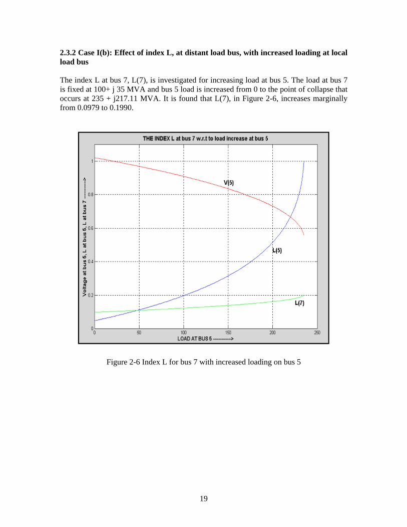
2.3.2 Case I(b): Effect of index L, at distant load bus, with increased loading at local load bus The index L at bus 7, L(7), is investigated for increasing load at bus 5. The load at bus 7 is fixed at 100+ j 35 MVA and bus 5 load is increased from 0 to the point of collapse that occurs at 235 + j217.11 MVA. It is found that L(7), in Figure 2-6, increases marginally from 0.0979 to 0.1990.

Figure 2-6 Index L for bus 7 with increased loading on bus 5

20

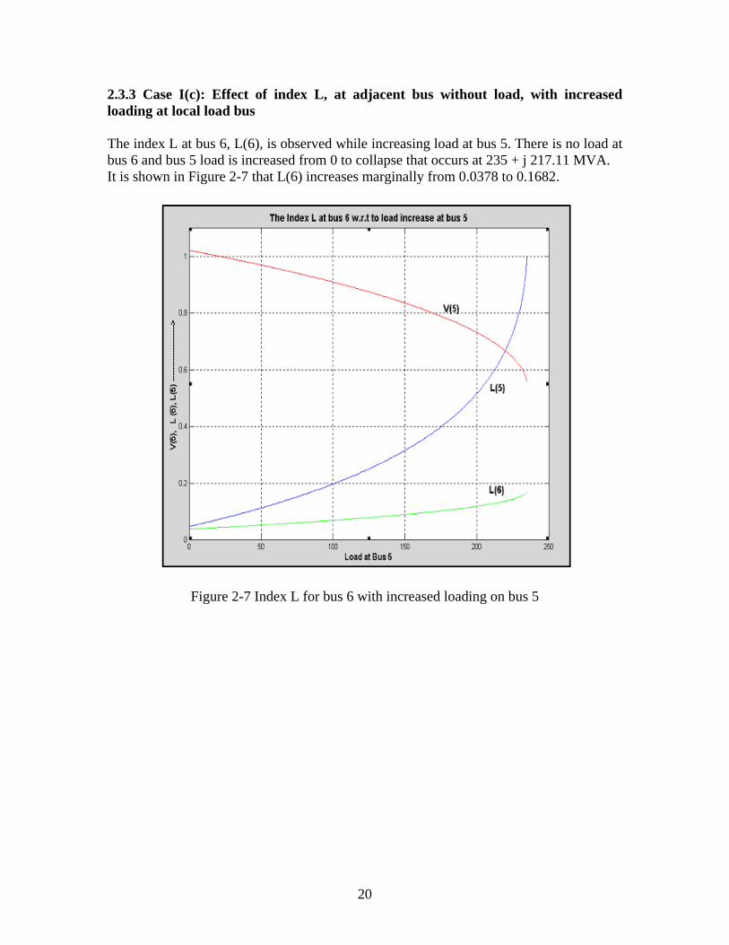
2.3.3 Case I(c): Effect of index L, at adjacent bus without load, with increased loading at local load bus The index L at bus 6, L(6), is observed while increasing load at bus 5. There is no load at bus 6 and bus 5 load is increased from 0 to collapse that occurs at 235 + j 217.11 MVA. It is shown in Figure 2-7 that L(6) increases marginally from 0.0378 to 0.1682.

Figure 2-7 Index L for bus 6 with increased loading on bus 5

21

2.3.4 Case II: Increasing load at bus 7 and observing the index L It is seen, in Figure 2-8 that index L approaches one at the collapse point. For this simulation, the load at bus 5 was 90 + j 30 MVA and load at bus 9 was 125 + j 50 MVA. The collapse occurs when the load at bus 7 is about 310.5+ j 286.86 MVA.


22

2.3.5 Case III: Increasing load at bus 9 and observing the index L As seen in Figure 2-9, the index L approaches one at the collapse point. For this simulation, the load at bus 5 was 90 + j 30 MVA and load at bus 7 was 100 + j 35 MVA. The collapse occurs when the load at bus 9 is about 251.5 + j 232.36 MVA.


2.3.6 Summary for the multi-bus scenarios 1) From the results of the simulations it can be distinctly observed that the index L for

the bus in a multi-bus system approaches unity (1) at the steady state voltage collapse point.

2) The index L incorporates the effect of the load at the bus it is calculated, as well as

the loading in the other parts of the system. However, the effect of other loads depends on how the bus under consideration is connected to the other buses.

3) There is no significant effect on the index value for a load bus that is not connected

directly to the bus where voltage is collapsing. 4) For a bus (such as bus 6 which has no load and no generation) that is connected to a

load bus (bus 5) on one end and a generator (bus 3) on the other end, the index (L(6) in this case) has only a marginal change as the load bus (bus 5) approaches collapse. This is because the voltage at that bus (bus 6) is being supported by the generator (at bus 3).

23

3 Dynamic Voltage Stability Issues 3.1 Applying index L to dynamic voltage stability studies In this sub-section, whether the index L can be used as an early indicator of a dynamic voltage stability limit is investigated. The disturbances investigated are (1) a large step load change and (2) sudden loss of a transmission line. The WSCC 9 bus system is used as a sample system to investigate the effects of dynamic voltage stability. This test system is the same one that was used in the previous chapter (shown in Figure 2-4) . The base case loadings for this simulation were:


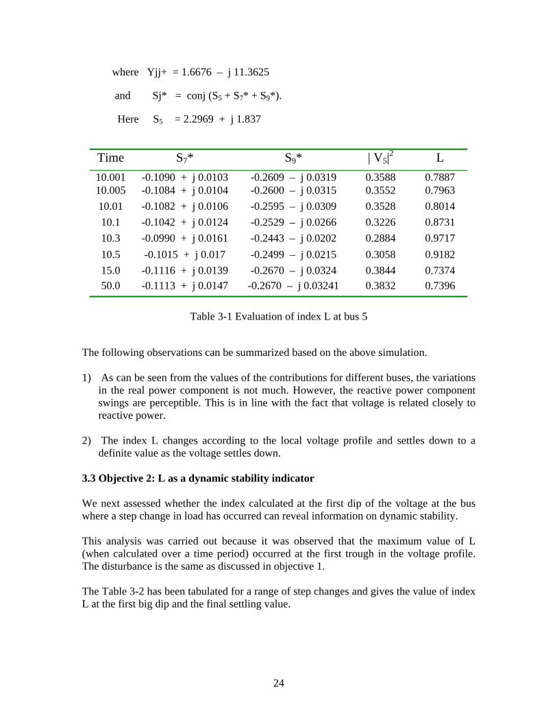
The simulations have been done in EUROSTAG. Models for the exciter and governor have been included in all the generator models. The L indices have been calculated on the same lines that discussed in the static voltage stability cases in the previous chapter. However, the voltages and the angles at the load buses are not the same during the dynamic time frame of interest. For simplicity, we have considered all the loads to be voltage and frequency independent. Since the voltage at the generator buses is not held constant during the dynamic situation, the index L at each generator bus is evaluated considering other generator buses as constant PV buses. The method of calculation is similar to the one adopted for load buses. The details of the analyses are given in the following sub-sections. In the simulations, only the governor and Automatic Voltage Regulator (AVR) have been modeled. Tap changers for transformers have not been incorporated. 3.2 Objective 1: Interaction of remote buses and local buses We investigated the contributions of remote bus loads (bus 7 and bus 9) on index L at a local bus (bus 5) with respect to time. Table 3-1 shows the quantities used for computing the index for a step change of load at bus 5 from 50 + j 40 to 229.69 + j 183.7 MVA. This disturbance was initiated at the time of 10.0 seconds. The index L is given by L = | Sj* / (Yjj+ x |V5|2) |

24

where Yjj+ = 1.6676 – j 11.3625

and Sj* = conj (S5 + S7* + S9*).

Here S5 = 2.2969 + j 1.837

Time S7* S9* | V5|2 L 10.001 -0.1090 + j 0.0103 -0.2609 – j 0.0319 0.3588 0.7887 10.005 -0.1084 + j 0.0104 -0.2600 – j 0.0315 0.3552 0.7963 10.01 -0.1082 + j 0.0106 -0.2595 – j 0.0309 0.3528 0.8014 10.1 -0.1042 + j 0.0124 -0.2529 – j 0.0266 0.3226 0.8731 10.3 -0.0990 + j 0.0161 -0.2443 – j 0.0202 0.2884 0.9717 10.5 -0.1015 + j 0.017 -0.2499 – j 0.0215 0.3058 0.9182 15.0 -0.1116 + j 0.0139 -0.2670 – j 0.0324 0.3844 0.7374 50.0 -0.1113 + j 0.0147 -0.2670 – j 0.03241 0.3832 0.7396

Table 3-1 Evaluation of index L at bus 5

The following observations can be summarized based on the above simulation. 1) As can be seen from the values of the contributions for different buses, the variations

in the real power component is not much. However, the reactive power component swings are perceptible. This is in line with the fact that voltage is related closely to reactive power.

2) The index L changes according to the local voltage profile and settles down to a

definite value as the voltage settles down. 3.3 Objective 2: L as a dynamic stability indicator We next assessed whether the index calculated at the first dip of the voltage at the bus where a step change in load has occurred can reveal information on dynamic stability. This analysis was carried out because it was observed that the maximum value of L (when calculated over a time period) occurred at the first trough in the voltage profile. The disturbance is the same as discussed in objective 1. The Table 3-2 has been tabulated for a range of step changes and gives the value of index L at the first big dip and the final settling value.

25

Power (MVA) First Negative Peak L Steady State L 50 + j 40 - 0.1135

200 + j 160 0.5224 0.4961 210 + j 168 0.5941 0.5548 220 + j 176 0.7002 0.6322 225 + j 180 0.7844 0.6818

229.6 + j 183.68 0.982 0.7396 229.65 + j 183.72 0.9963 0.7396 229.67 + j 183.736 1.0037 0.7396 229.68 + j 183.744 1.0109 0.7396

Table 3-2 Index L at the first big dip and the final settling value

The following observations can be made out based on this simulation. 1) Looking at the data of the power contributions from other load buses (buses 7 and 9

in our case) to the index calculated at the reference bus (bus 5 in our case), it is observed that the active component remains substantial even at higher loads compared with the initial value. However, considerable effect is reflected on the reactive power contributions. For example, at a load change from 50 + j 40 to 225 + j 180 at bus 5, the real part of S9

* changed from 0.3421 to 0.2626. However, the reactive contribution dropped sharply from 0.1106 to 0.0367. This suggests two observations.

a) The voltage at the bus nearing voltage collapse is strongly influenced by the

reactive power demand at its bus. b) The effect of reactive power contributions of other load buses to the index is

minimal. This supports our understanding that voltage collapse starts as a local phenomenon at a particular overloaded voltage bus (which is influenced strongly by its local reactive power requirement).

2) It is observed that the largest value of the index, which happens to occur at the first

trough of the voltage after the load change, approaches one at the dynamic voltage collapse point. The final value of the index L matches with the value which was calculated for the steady state voltage stability case.

26

3.4 Objective 3: L as an overall system profile indicator We next investigated the overall profile of the index variations at all load buses and all generator buses during a particular step load disturbance in one load bus. A load change from 50 + j 40 to 229.6 + j 183.68 was imposed on load bus 5 at time = 10 seconds. The results for the evaluation of the indices as seen from the different buses are given below. (a) Figure 3-1 shows the variations of all the indices with respect to time following the

disturbance.

Figure 3-1 Variations of all the indices with respect to time

27

(b) Figure 3-2 includes the voltage and index variations for all load buses with respect to time, following the disturbance.

Figure 3-2 Voltage and index variations for all load buses

28

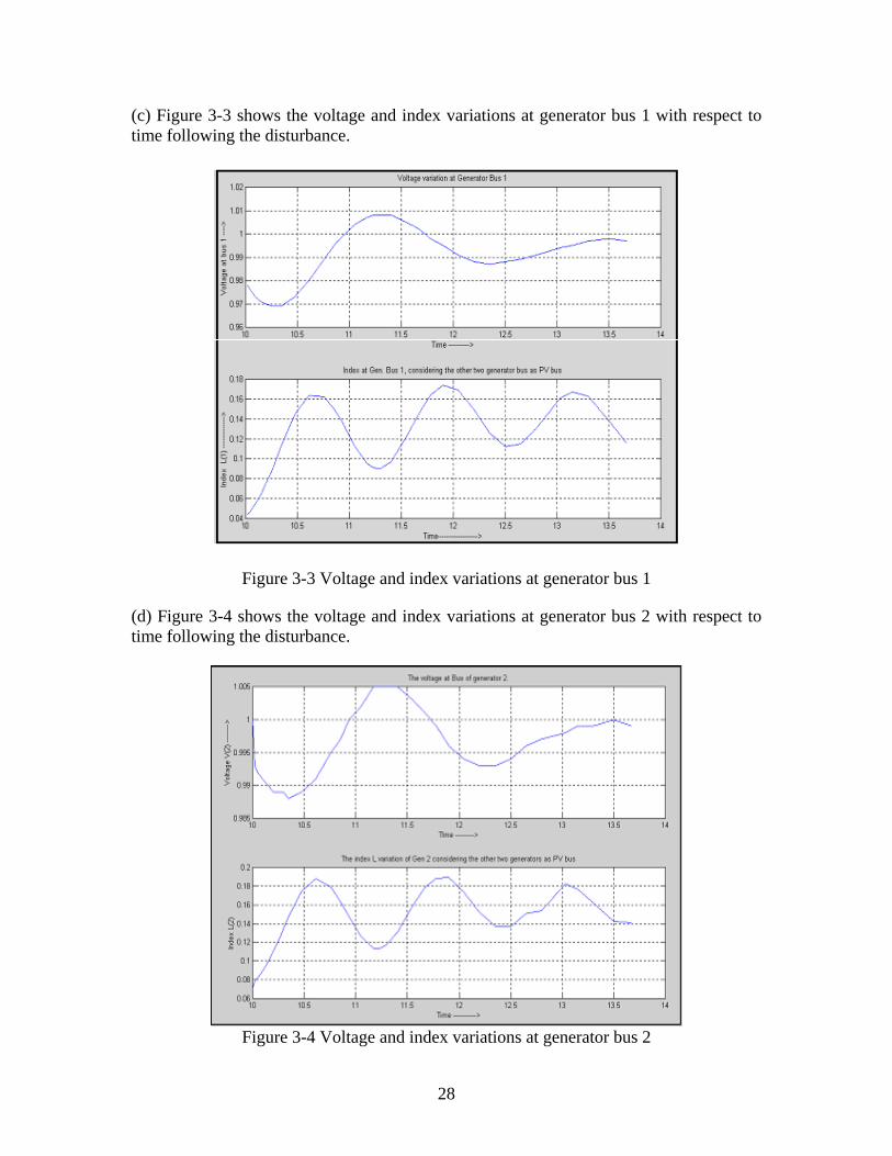
(c) Figure 3-3 shows the voltage and index variations at generator bus 1 with respect to time following the disturbance.

Figure 3-3 Voltage and index variations at generator bus 1

(d) Figure 3-4 shows the voltage and index variations at generator bus 2 with respect to time following the disturbance.


29

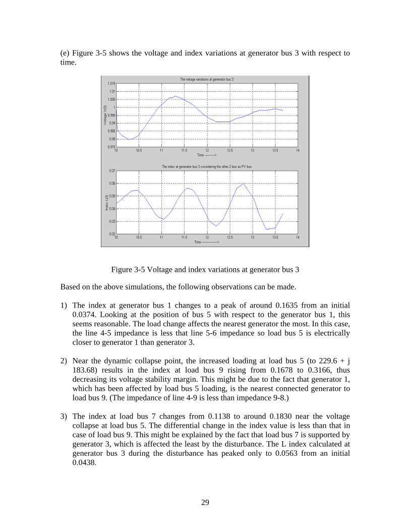
(e) Figure 3-5 shows the voltage and index variations at generator bus 3 with respect to time.


Based on the above simulations, the following observations can be made. 1) The index at generator bus 1 changes to a peak of around 0.1635 from an initial

0.0374. Looking at the position of bus 5 with respect to the generator bus 1, this seems reasonable. The load change affects the nearest generator the most. In this case, the line 4-5 impedance is less that line 5-6 impedance so load bus 5 is electrically closer to generator 1 than generator 3.

2) Near the dynamic collapse point, the increased loading at load bus 5 (to 229.6 + j

183.68) results in the index at load bus 9 rising from 0.1678 to 0.3166, thus decreasing its voltage stability margin. This might be due to the fact that generator 1, which has been affected by load bus 5 loading, is the nearest connected generator to load bus 9. (The impedance of line 4-9 is less than impedance 9-8.)

3) The index at load bus 7 changes from 0.1138 to around 0.1830 near the voltage

collapse at load bus 5. The differential change in the index value is less than that in case of load bus 9. This might be explained by the fact that load bus 7 is supported by generator 3, which is affected the least by the disturbance. The L index calculated at generator bus 3 during the disturbance has peaked only to 0.0563 from an initial 0.0438.

30

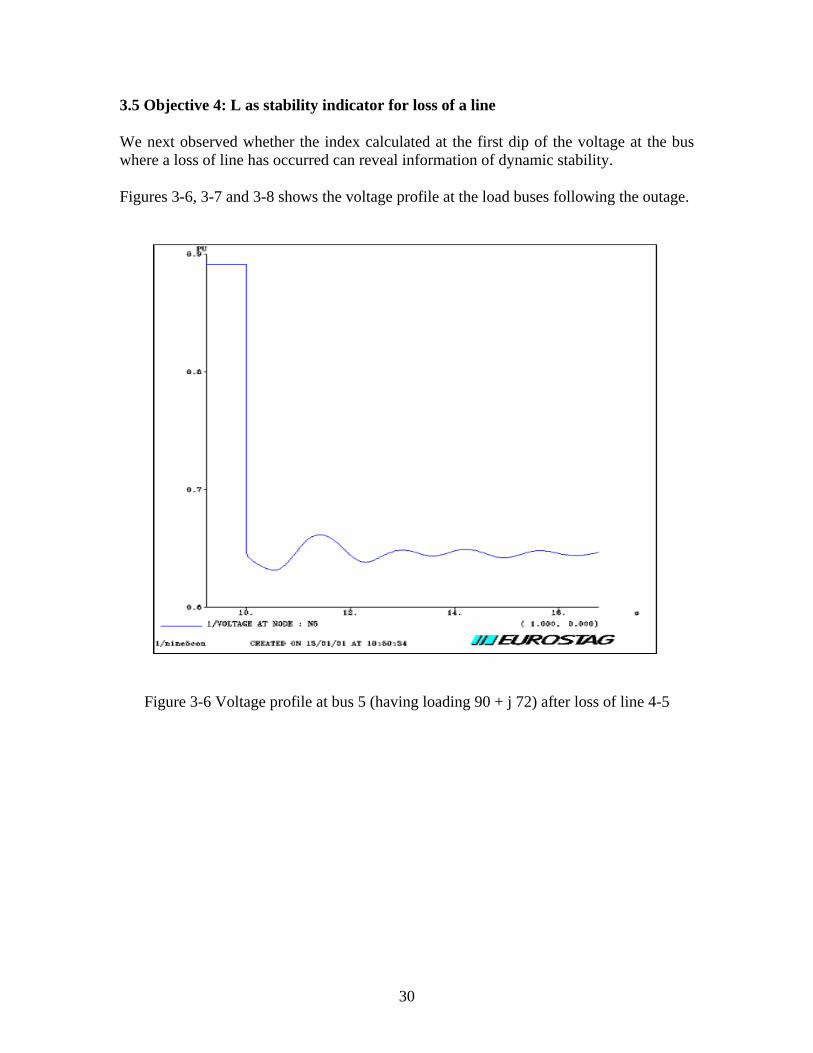
3.5 Objective 4: L as stability indicator for loss of a line

We next observed whether the index calculated at the first dip of the voltage at the bus where a loss of line has occurred can reveal information of dynamic stability. Figures 3-6, 3-7 and 3-8 shows the voltage profile at the load buses following the outage.

Figure 3-6 Voltage profile at bus 5 (having loading 90 + j 72) after loss of line 4-5

31

Figure 3-7 Voltage profile at bus 7 after loss of line 4-5

Figure 3-8 Voltage profile at bus 9 after loss of line 4-5

32

Tables 3-3, 3-4 and 3-5 show the index calculated (1) at the time of the largest dip (negative peak) in the voltage profile observed at bus 5, and (2) after the voltage oscillations dies down (i.e., steady state).

Power (MVA) First Negative Peak L Steady State L 50 + j 40 0.2312 0.2300 70 + j56 0.3706 0.3666 80 + j 64 0.4801 0.4722 90 + j 72 0.6787 0.6502

93 + j 74.4 0.8093 0.7508 93.5 + j 74.8 0.8645 0.7741 93.75 + j 75.0 0.8690 0.7860 93.9 + j 75.12 0.8850 0.7950

93.96 + j 75.168 0.8920 0.7980 93.97 + j 75.176 0.8951 0.7980

Table 3-3 Evaluation of index for bus 5 after loss of line 4-5

Power (MVA) First Negative Peak L Steady State L

50 + j 40 0.1241 0.1240 70 + j56 0.1370 0.1365 80 + j 64 0.1457 0.1448 90 + j 72 0.1584 0.1565

93 + j 74.4 0.1650 0.16194 93.5 + j 74.8 0.1670 0.1630 93.75 + j 75.0 0.1681 0.1634 93.9 + j 75.12 0.1689 0.164

93.96 + j 75.168 0.1690 0.1641 93.97 + j 75.176 0.1690 0.1641


Power (MVA) First Negative Peak L Steady State L

50 + j 40 0.1538 0.1541 70 + j56 0.1568 0.1573 80 + j 64 0.1592 0.1594 90 + j 72 0.16237 0.1627

93 + j 74.4 0.16399 0.16383 93.5 + j 74.8 0.16457 0.1640 93.75 + j 75.0 0.1647 0.1644 93.9 + j 75.12 0.1651 0.1645

93.96 + j 75.168 0.1652 0.1645 93.97 + j 75.176 0.1652 0.1645


33

3.5.1 Graphical plots for objective 4: L as stability indicator for loss of a line

(1) The Figure 3-9 shows the variations of the index at the load bus 5 with respect to its bus loading. Two curves are show: the peak index L (which occurs at the first largest negative dip in the voltage at bus 5 following the loss of line 4-5), and the index L evaluated after the voltage stabilizes down after the disturbance.

Figure 3-9 Variations of the index at load bus 5

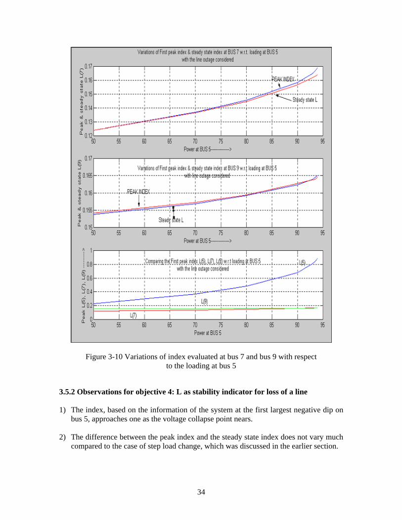
(2) Figure 3-10 shows the variations of indices evaluated at bus 7 and bus 9 with respect to the loading at bus 5. The peak value (evaluated at the first largest negative dip in the voltage at bus 5 following the disturbance) and the steady state index value are plotted.

34

Figure 3-10 Variations of index evaluated at bus 7 and bus 9 with respect to the loading at bus 5

3.5.2 Observations for objective 4: L as stability indicator for loss of a line 1) The index, based on the information of the system at the first largest negative dip on

bus 5, approaches one as the voltage collapse point nears. 2) The difference between the peak index and the steady state index does not vary much

compared to the case of step load change, which was discussed in the earlier section.

35

3) The bus 5 collapsed around a load value of 94 + j75.2 dynamically because of line outage 4-5. The load at the steady state voltage stability limit evaluated for this case was 96.4 + j 89.06. Thus, the dynamic voltage stability limit calculated on the basis of a line outage is less than the steady state voltage stability limit.

4) The increase in index at buses 7 and 9 following loss of line 4-5 is marginal. This is

because the line 4-5 outage does not directly influence these load centers. Moreover, since the real load at bus 5 is only about 0.9 p.u during its dynamic collapse, the impact of its transferred effect to load bus 7 and 9 is also minimal.

3.6 Objective 5: Impacts of Z on L as an indicator We also investigated whether for the loss of line case for dynamic stability evaluation, the index calculated on the basis of exact local Zii term (considering the loss of line information), but with other impedance terms remaining the pre-contingency value, can still give a sufficiently accurate index calculation. Tables 3-6, 3-7 and 3-8 give the result of calculating index considering the effect of the lost line 4-5 in calculating the ZLL matrix, (stated as “Exact”), and taking only the Zii term taking the lost line 4-5 into consideration while the rest of the terms as the original healthy state ZLL matrix. (stated as “Approximate”).

Power (MVA) Exact Peak Index

Approximate Peak L

Exact Steady Index

Approximate Steady L

50 + j 40 0.2312 0.2451 0.2300 0.2437 70 + j56 0.3706 0.3844 0.3666 0.3801 80 + j 64 0.4801 0.4938 0.4722 0.4855 90 + j 72 0.6787 0.6921 0.6502 0.6632

93 + j 74.4 0.8093 0.8228 0.7508 0.7636 93.5 + j 74.8 0.8645 0.8601 0.7741 0.7868 93.75 + j 75.0 0.8690 0.8826 0.7860 0.7988 93.9 + j 75.12 0.8850 0.8990 0.7950 0.8076

93.96 + j 75.168 0.8920 0.9056 0.7980 0.8107 93.97 + j 75.176 0.8951 0.9088 0.7980 0.8108

Table 3-6 Evaluation of index for bus 5

36

Power (MVA) Exact Peak

Index Approximate

Peak L Exact Steady

Index Approximate

Steady L 50 + j 40 0.1241 0.1174 0.1240 0.1174 70 + j56 0.1370 0.1254 0.1365 0.1251 80 + j 64 0.1457 0.1310 0.1448 0.1302 90 + j 72 0.1584 0.1389 0.1565 0.1376

93 + j 74.4 0.1650 0.1433 0.16194 0.1410 93.5 + j 74.8 0.1670 0.1445 0.1630 0.1417 93.75 + j 75.0 0.1681 0.1451 0.1634 0.1419 93.9 + j 75.12 0.1689 0.1456 0.164 0.1423

93.96 + j 75.168 0.1690 0.1457 0.1641 0.1423 93.97 + j 75.176 0.1690 0.1458 0.1641 0.1423


Power (MVA) Exact Peak

Index Approximate

Peak L Exact Steady

index Approximate

Steady (L) 50 + j 40 0.1538 0.1695 0.1541 0.1693 70 + j56 0.1568 0.1791 0.1573 0.1794 80 + j 64 0.1592 0.1855 0.1594 0.1853 90 + j 72 0.16237 0.1941 0.1627 0.1937

93 + j 74.4 0.16399 0.1986 0.16383 0.1970 93.5 + j 74.8 0.16457 0.1999 0.1640 0.1980 93.75 + j 75.0 0.1647 0.2004 0.1644 0.1983 93.9 + j 75.12 0.1651 0.2012 0.1645 0.1985

93.96 + j 75.168 0.1652 0.2013 0.1645 0.1986 93.97 + j 75.176 0.1652 0.2014 0.1645 0.1986


37

Figure 3-11 Index L value computed exactly and after approximation The following observations can be made based on this simulation. 1) The Exact and the Approximate values match closely for all the load buses. Thus, the

index is predominantly dependent on the term Zii of the ZLL matrix. 2) If any local measurement at load buses can yield this value, then the index L

calculated would be fairly approximate to the exact value, even if we cannot get the complete information of all the healthy lines in the network.

3.7 Publications The readers can refer to reference [4] for summary of the work that has been discussed in the earlier sections of this chapter. The dynamic modeling of generators, governors, ULTC, switched capacitor and loads using EUROSTAG have also been carried to study dynamic voltage stability [8]. The various myths surrounding dynamic voltage stability have been clarified here. Moreover, the importance of dynamic reserves of generation to maintain voltage stability during a dynamic disturbance has been clearly demonstrated in the simulations. Interested readers may refer to publication [8] for details about the simulation and the summary of the results.

38

4 Voltage Stability Constrained OPF Algorithm As demonstrated in Chapter 3, the voltage stability index L represents, in a way, how far the load bus is from the voltage collapse point. This feature can be exploited in developing a load curtailment policy incorporating the security feature of voltage stability margin. The following section proposes a method to achieve this. 4.1 Algorithm The following steps explain the procedure of carrying out an optimal power flow (OPF) with the index Li at load buses as one of the constraints. The objective function is minimization of load curtailed, or

For all buses from i =1,2…n

For each bus i, the term Load-Curtailmenti is given by the following expression:

Here Plireq is the load demand that is to be satisfied at bus i before the OPF procedure. Pli is the load demand that can actually be met, within the constraint specified, after the OPF. For all the buses, the power flow equations to be satisfied are:

The minimum and maximum limits on generators active and reactive power output is given by:

The transmission line constraints can be specified by,

i

n

itCurtailmenLoadimizemin −∑

=1

lilireqi PPtCurtailmenLoad −=−

01

=δ+δ−− ∑=

)sinBcosG(VVPP ijijijijj

n

jiligi

01

=δ−δ−− ∑=

)cosBsinG(VVQQ ijijijij

n

jjiligi

maxgigimingi PPP ≤≤

maxgigimingi QQQ ≤≤

39

The load shedding philosophy can be simplified if we assume that shedding is carried out in equal proportion of active and reactive power. In other words, the power factor of all the loads remains the same as the initial value. This can be represented as:

The following constraints are added to the OPF formulation to incorporate voltage stability. (a) For all buses i, include the following constraints, as usually found in OPF formulations.

(b) For all the load buses (PQ) and buses where there are no loads and generators i, use the following additional constraint, based on local index calculation Li.

4.2 An illustration The WSCC 9 bus system is taken as a sample system to illustrate the applicability of the indicator L to a multi-bus system. The test system is the same one that was used in section 2.2.1. The following loads are in the system:


Table 4-1 gives the result of the OPF run based on the proposed algorithm for the above case. There is no load curtailment on bus 7 and bus 9. Only bus 5 has load curtailment. NOTE: All the PV buses are held at V = 1.0 p.u.

lireqlilireqli QQPP // =

lireqli PP ≤≤0lireqli QQ ≤≤0

maxiimini VVV ≤≤

222maxijijij SQP ≤+

criti LL ≤

40

Lcrit for all the load buses Load curtailment at bus 5

0.1 90.57 + j 72.45 0.2 36.45 + j 291.6 0.25 26.51 + j 21.21

Table 4-1 Results after the OPF

Without the constraint of voltage stability index imposed on the load buses, the load curtailment value at bus 5 after running OPF was found to be 26.51 + j 21.21. 4.3 Observations 1) For the above case, if we choose any value of Lcrit just above 0.21, the voltage

stability index constraint does not seem to affect the OPF solution for our load pattern and system chosen. This is because the constraint Vmin is already violated and, hence, is held constant at the violated bus. Thereafter, the algorithm stops searching for a solution based on the voltage stability index constraint criterion.

2) The choice of a low value of Lcrit increases the required load curtailment. Therefore,

the above OPF algorithm encompasses the security-based feature of voltage stability in the calculation of load curtailment.

3) If the allowable Vmin for bus 5 were kept as 0.8 p.u., the load curtailment using the

stability margin criterion for Lcrit of 0.3 was found out to be more than that calculated without using it.

4.4 Publications For interested readers, further simulation and application details of the algorithm can be obtained from reference [1]. The authors have also formulated the algorithm to incorporate FACTS devices such as TCSC, the detail of which can be obtained from reference [2]. The loadability of the system can be increased by using these devices. The voltage stability constrained OPF algorithm, developed in this project, blends itself effectively to the steady state characteristic of the devices within its formulation. Application of the algorithm to composite reliability analysis has been explored in reference [3]. Evaluation of reliability indices that incorporates the steady state voltage stability could be achieved using the algorithm.

41

5 Transaction-Based Stability Margin and Utilization Factors Evaluation 5.1 Theory behind transaction-based power flow To derive a more complete formula of decomposition, we begin with the coupled AC power flow equations in polar form as follows.

=−−−

=+−−

∑

∑

∈

∈

0)cossin()(

0)sincos()(

ijijijijijiDiGi

ijijijijijiDiGi

bgVQQ

bgVPP

θθ

θθ (5.1)

For ni ...,2,1= )( si ≠ ( s is the slack bus), GiGi QP , are active and reactive power generations at bus i ; DiDi QP , are active and reactive power loads at bus i ; iiV θ∠ is the voltage magnitude and angle of bus i ; jiij θθθ −= ; ijijij jbgy += is the branch admittance between nodes i and j .

Let ),( θV be the solution of the power flow equations (5.1). Several basic facts with respect to a general transmission system are observed below.

(1) Line resistance is considered much smaller than line reactance (i.e., r/x <<1), and

voltage angle differences across each branch are assumed to be small.

(2) Active power flows in the system are strongly coupled with voltage angle differences across branches.

(3) Reactive power flows in the system are strongly coupled with the voltage magnitudes

V throughout the entire network.

(4) When the absolute value of voltage angle θ is small enough throughout the system, nodal imaginary current components are strongly coupled with the voltage magnitudes V.

Facts 1, 2 and 3 are widely recognized, and used in DC flow analysis and other linearized flow models. In general Fact 4 holds on the conditions r/x≤1/3 and |θ|≤ π/9, which is rather straightforward from the nodal voltage and current equation.

42

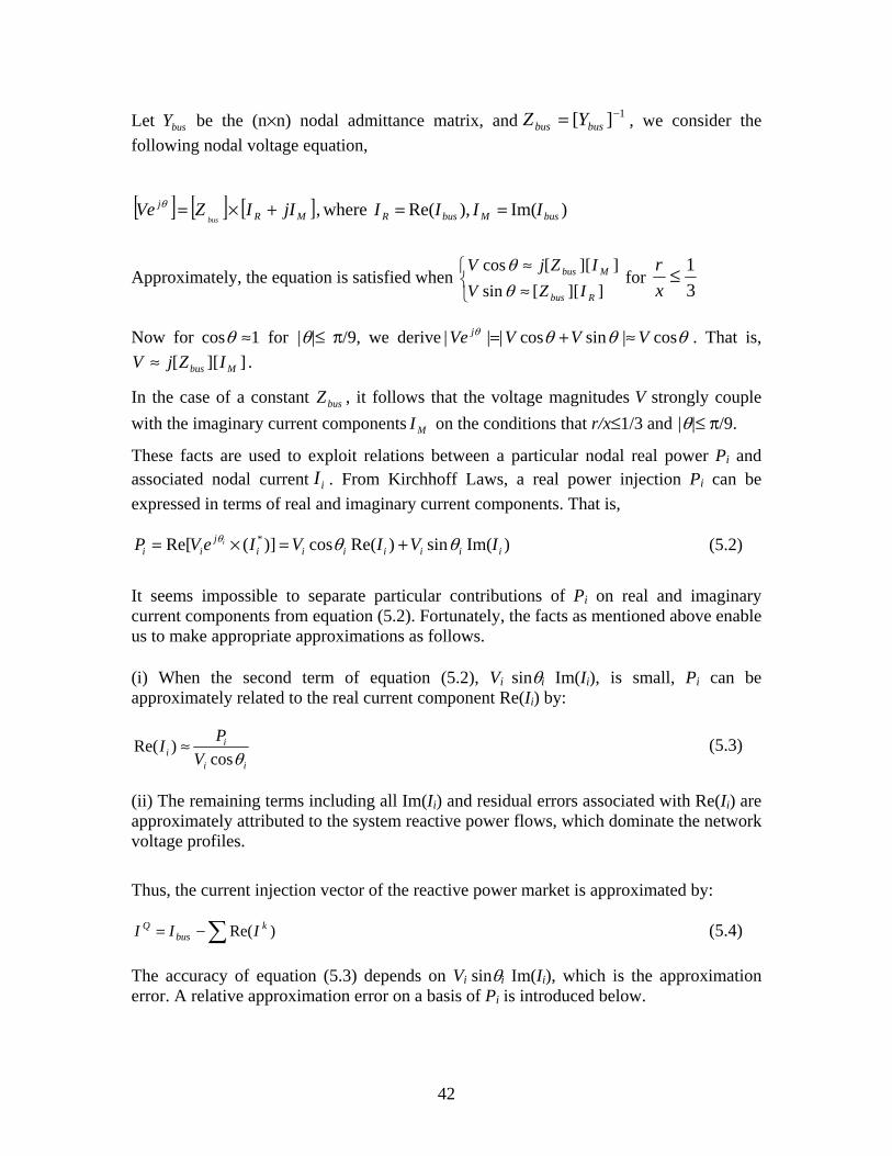
Let busY be the (n×n) nodal admittance matrix, and 1][ −= busbus YZ , we consider the following nodal voltage equation,

[ ] [ ] [ ] )Im(),Re( where, busMbusRMRj IIIIjIIZVe

bus==+×=θ

Approximately, the equation is satisfied when

≈≈

]][[sin]][[cos

Rbus

Mbus

IZVIZjV

θθ

for 31≤

xr

Now for θcos ≈1 for |θ|≤ π/9, we derive θθθθ cos|sincos||| VVVVe j ≈+= . That is, ]][[ Mbus IZjV ≈ .

In the case of a constant busZ , it follows that the voltage magnitudes V strongly couple with the imaginary current components MI on the conditions that r/x≤1/3 and |θ|≤ π/9.

These facts are used to exploit relations between a particular nodal real power Pi and associated nodal current iI . From Kirchhoff Laws, a real power injection Pi can be expressed in terms of real and imaginary current components. That is,

)Im(sin)Re(cos)](Re[ *iiiiiii

jii IVIVIeVP i θθθ +=×= (5.2)

It seems impossible to separate particular contributions of Pi on real and imaginary current components from equation (5.2). Fortunately, the facts as mentioned above enable us to make appropriate approximations as follows.

(i) When the second term of equation (5.2), Vi sinθi Im(Ii), is small, Pi can be approximately related to the real current component Re(Ii) by:

ii

ii V

PIθcos

)Re( ≈ (5.3)

(ii) The remaining terms including all Im(Ii) and residual errors associated with Re(Ii) are approximately attributed to the system reactive power flows, which dominate the network voltage profiles.

Thus, the current injection vector of the reactive power market is approximated by:

∑−= )Re( kbus

Q III (5.4)

The accuracy of equation (5.3) depends on Vi sinθi Im(Ii), which is the approximation error. A relative approximation error on a basis of Pi is introduced below.

43

i

iiiiiiiPi PIVE

ϕθϕθθ

cos)sin(sin/)Im(sin −−== (5.5)

EPi depends on the phase angle iθ and power factor (PF) angle iϕ . To secure dynamic reactive power reserves, the normal PF on the demand side is restricted to a narrow margin (say 90.0cos ≥ϕ in lagging). Two approximation error levels are marked:

Level 1: |EPi |≤ 0.065, for 155.6 ≤≤− iθ deg. Level 2: |EPi |≤ 0.115, for 2010 ≤≤− iθ deg.

Given a range of 2010 ≤≤− θ degrees, the largest approximation error is around 10 percent. For example, from a standard power flow solution, a range of appropriate reference angles to reduce approximation errors can be determined by:

maxmax,minmin, θθθθθ −≤≤− LsL (5.6)

where minmax ,θθ are the largest and smallest phase angles corresponding to a zero

reference angle; and max,min, , LL θθ are the lower and upper limits of Level 1 or 2. 5.2 Transaction-based power flow algorithm 5.2.1 Assumptions To begin with the decomposition algorithm, we first introduce economic contexts and involved assumptions.

(1) An energy market consists of individual energy scheduling coordinators SCk, who are entitled to arrange MW exchange schedules and to choose loss suppliers.

(2) A SCk may not maintain its own reactive power balance. Instead, a separate market

named Q, the central and ISO-dependent reactive power scheduling is responsible for the reactive power support.

(3) A SCk is also responsible for a portion of transmission losses resulting from

consuming reactive power support, which introduces reactive power flows.

5.2.2 Step-wise procedures for decomposition

We derive the decomposition equations on a general power system with N-buses and L-branches. To simplify our presentation, we assume only two market players in the system: PX is a central power exchange market; and TX is a bilateral transaction. These

44

assumptions will be relaxed later. A system-wide reactive power market Q conducted by the ISO is responsible for overall reactive support services.

Step1: Select an appropriate angle for the slack bus from the given power flow solution, referring to equation (5.6).

Step 2: Decompose the nodal current vector based on TXs.

From a known operating point ),( θV , the (n×1) nodal current vector busI is determined by:

][ busbusbus EYI ×= , where

=i

i

jn

j

bus

eV

eVE

θ

θ

. 1

(5.7)

where busY is the (n×n) nodal admittance matrix, which is nonsingular in consideration of line charging and other shunt terms. According to the proposed approximation equation (5.3), busI is decomposed into individual market components. That is,

−

−

=

nn

PXnD

PXnG

ii

PXiD

PXiG

PX

VPP

VPP

I

θ

θ

cos

.

.cos

.

,,

,,

−=

0cos

0cos

0

,

,

mm

TXmD

kk

TXkG

TX

VP

VP

I

θ

θ TXPXbusQ IIII −−= (5.8)

where kk SCD

SCG PP ∗∗ ,, , are the active power generations and loads at bus i , in association with

PX or TX. TX is with the source and sink buses at k and m respectively.

Step 3: Decomposed nodal voltage components immediately follow from Step 2 by Kirchhoff Laws.

)(][ *1∗

−∗ ×= IYE bus (5.9)

where the subscript symbol ∗ means PX, TX or Q individually. Normally,

≈≈ |||| busQ EE 1 0|| ≈PXE 0|| ≈TXE (5.10)

45

Step 4: Compute branch current components ijji II _*,*, ,− on any link between buses i and j by substituting the decomposed bus voltage vectors *E of equation (5.9) into the branch current equations as follows.

In terms of a transmission line, or a transformer with a ratio 1.0, the decomposed branch current components directed from the buses i to j are derived by:

)()( ,,,0,*, ijijjiliji jbgEEbEI +×−+= ∗∗∗− (5.11)

)()( ,,,0,*, ijijijljij jbgEEbEI +×−+= ∗∗∗− (5.12)

where lb is the half line shunt susceptance. The symbol ∗ means PX, TX or Q individually. For other branches, such as transformers with non-standard ratios (i.e., ijt ≠1.0), their branch currents can be derived easily.

Step 5: Decompose complex power flows over each branch. For example, in terms of a branch between buses i and j , the complex power flow with respect to “from” bus of the branch is:

*, jiibusji IES −− ×= (5.13)

Further, it can be rewritten as

term6*,,

term5*,,

term4*,,

*,,

term3*,,

term2*,,,

term1*,,,

*,,,,,,

)(

)()(

)()(

thjiQiTX

thjiQiPX

thjiPXiTXjiTXjiPX

rdjiQiQ

ndjiTXiTXiQ

stjiPXiPXiQ

jiTXjiPXjiQiTXiPXiQji

IEIE

IEIEIE

IEEIEE

IIIEEES

↵−

↵−

↵−−−

↵−

↵−

↵−

−−−−

++

+++

+++=

++×++=

(5.14)

where iQiTXiPXibus EEEE ,,,, ,,, is the ith element of the voltage vectors QTXPXbus EEEE ,,, individually. We categorize terms of equation (5.14) as follows:

• The 1st, 2nd and 3rd terms are major components attributed to PX, TX and Q markets respectively.

• The 4th term represents an interacting component between energy markets PX and TX.

46

• The 5th and 6th terms represent interacting component between PX/TX and Q markets separately.

Evidently, the market players PX and TX account for self-induced terms, and also take care of the interacting cross-terms. Moreover, there is a flexibility to allocate the interactive component between PX and TX, which can be designed into market rules. Therefore, we the complex flow decomposition equation for one branch directed from i to j as follows.

jiQjiTXjiPXji SSSS −−−− ++= ,,, (5.15)

where

)()( *,,

*,,

*,,

*,,,, jiPXiTXjiTXiPXTXPXjiQiPXjiPXiPXiQjiPX IEIEfIEIEES −−−−− +×++×+= ω

)()( *,,

*,,

*,,

*,,,, jiPXiTXjiPXiTXTXTXjiQiTXjiTXiTXiQjiTX IEIEfIEIEES −−−−− +×++×+= ω

*,,, jiQiQjiQ IES −− =

PXTXTXPX ff ωω , are sharing factors imposed upon PX and TX for their interactive component. 1≡+ PXTXTXPX ff ωω . Along the same line, the complex power flow with respect to “to” bus of the branch can be decomposed into the following market components:

ijQijTXijPXij SSSS −−−− ++= ,,, (5.16)

where

)()( *,,

*,,

*,,

*,,,, jiPXiTXjiTXiPXTXPXjiQiPXjiPXiPXiQjiPX IEIEfIEIEES −−−−− +×++×+= ω

)()( *,,

*,,

*,,

*,,,, jiPXiTXjiTXiPXPXTXjiQiTXjiTXiTXiQjiTX IEIEfIEIEES −−−−− +×++×+= ω

*,,, jiQjQijQ IES −− =

Further, the decomposed real flow, real loss, reactive flow and reactive loss components on the branch immediately follow from the solved complex power flow components

ijji SS −− *,*, , . In particular,

)Re(21

*,*,(*), ijjijiflow SSP −−− −= (5.17)

47

)Re( *,*,(*), ijjijiloss SSP −−− += (5.18)

)Im(21

*,*,(*), ijjijiflow SSQ −−−−= (5.19)

)Im( *,*,(*), ijjijiloss SSQ −−− −= (5.20)

where * means PX, TX or Q individually.

Step 6: Distribute the portion of transmission loss arising from reactive power delivery to the energy customers in proportion to their reactive power usage.

The intent of reactive power scheduling is to balance the system reactive loads and MVAr losses mainly generated from interzonal power transfers. The transmission losses incurred from reactive power flows only takes up a small percent of the system losses under normal operating conditions. Therefore, we reallocate it between PX and TX in proportion to their reactive power usage.

∑∑ ∑∑

∑∑−

=−

∈

−∈ ×

+

+=∆

LjiQloss

TXPXk Ljikloss

NiiDk

Ljiloss

NiiD

QL PQQ

QQP ),(

,),(,

(*),*,

)(*, (5.21)

where * denotes energy interchange schedules PX or TX. Eventually, the transmission loss charges to PX and TX are:

),(),()( QPXLL

jiPXlossPXL PPP ∆+=∑ − (5.22)

∑ ∆+= −L

QTXLjiTXlossTXL PPP ),(),()( (5.23)

Thus, all transmission losses are distributed among energy transactions independent of the reactive power market clearing system.

Step 7: Adjust loss shares among the market players by an iteration scheme. As only a relatively small number of generators are used for load following purposes in a power system, the loss generated from a PX or a bilateral transaction is likely to be supplied by a third party, not necessarily the same generator serving the load. Accordingly, an adjustment process is needed to take care of the loss. For example, suppose TX decides to buy the loss from a third party generator (say s ), then a small

48

amount of generation from the supplier s is attributed to the TX, which corresponds to the allocated loss reflected in equation 5.23. We adjust the current vector TXI accordingly, and repeat Steps 2 through 6 again. This adjustment scheme can be extended for a PX market similarly. Under normal operating conditions, the loss adjustment process converges in a few iterations. It is straightforward to generalize to cases with a large number of the TXs. For any kSC , the complex power flow contributions to one branch between the buses i and j are:

∑−∈

−−

−−−

+×+

+×+=

kThjiSCiSCjiSCiSCSCSC

jiQiSCjiSCiSCiQjiSC

khhkhk

kkkk

IEIEf

IEIEES

)(

)(

,,,,

,,,,,,

ω (5.24)

and

∑−∈

−−

−−−

+×+

+×+=

kThijSCjSCijSCjSCSCSC

ijQjSCijSCjSCjQijSC

khhkhk

kkkk

IEIEf

IEIEES

)(

)(

,,,,

,,,,,,

ω (5.25)

where T is the number of all energy scheduling coordinators including all the TXs and PXs.

5.3 Transaction-based voltage security margin allocation algorithm Integrating the TBPF [10] and the index L would lead to a transaction-based voltage security utilization algorithm [5] that is formulated in the following section. To simplify our presentation, we assume only two types of market players in the system: PX represents one central power exchange market, and TX represents a set of TN bilateral transactions. A system-wide reactive power market Q conducted by the ISO is responsible for overall reactive support services. Step 1: Decompose the nodal current vector based on TXs.

][ busbusbus EYI ×= , where

=i

i

jn

j

bus

eV

eVE

θ

θ

. 1

(5.26)

49

−

−

=

nn

PXnD

PXnG

ii

PXiD

PXiG

PX

VPP

VPP

I

θ

θ

cos

.

.cos

.

,,

,,

T

mm

TXmD

kk

TXkG

jTX Nj

VP

VP

Ij

j

,....,1

0cos

0cos

0

)(

)(

,

,

)( =

−=

θ

θ

)(

1

jTX

N

jPXbusQ IIII

T

∑=

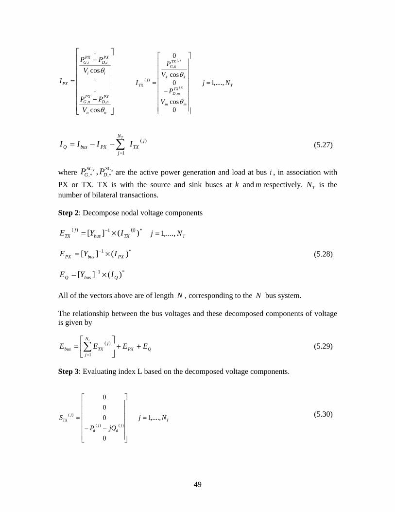
−−= (5.27)

where kk SCD

SCG PP ∗∗ ,, , are the active power generation and load at bus i , in association with

PX or TX. TX is with the source and sink buses at k and m respectively. TN is the number of bilateral transactions. Step 2: Decompose nodal voltage components

)(][ *(j)1)(TXbus

jTX IYE ×= −

TNj ,....,1=

)(][ *1PXbusPX IYE ×= − (5.28)

)(][ *1QbusQ IYE ×= −

All of the vectors above are of length N , corresponding to the N bus system. The relationship between the bus voltages and these decomposed components of voltage is given by

QPX

N

j

jTXbus EEEE

t

++

= ∑

=1

)( (5.29)

Step 3: Evaluating index L based on the decomposed voltage components.

Tj

dj

d

jTX Nj

jQPS ,....,1

0

000

)()(

)( =

−−= (5.30)

50

−−

−−

=

nn dd

dd

PX

jQP

jQP

S...

11

(5.31)

Considering PX transaction as the first one, the index L is given by the following expression:

2

jPXjj

jPXj

VY

SL+

+

∗

= , (5.32)

where jcorrjPXj SSS +=+ , jPX

jiLi

iPX

iPX

jj

jijcorr V

V

S

Z

ZS

= ∑

≠∈

∗

∗

, jj

jj

ZY 1=+

and QPXPX EEV += .

Here j represents all the load buses.

By reflecting the appropriate changes in the +jS and PXV terms of the previous expression, the index can be evaluated after adding each bilateral transaction TX one after the other. For example, the index after adding the first transaction TX to the PX would be given by

2

)( )1(

)1(

jTXPXjj

jTXPXj

VY

SL

++

+

∗

+ = , (5.33)

where jcorrjTXjPXj SSSS ++=+)1( , jTXPX

jiLi

iTXPX

iPX

jj

jijcorr V

V

S

Z

ZS )(

)(

)1(

)1(

+

≠∈

+

∗

∗

= ∑ ,

and )1()( )1(

TXQPXTXPX EEEV ++=+ .

51

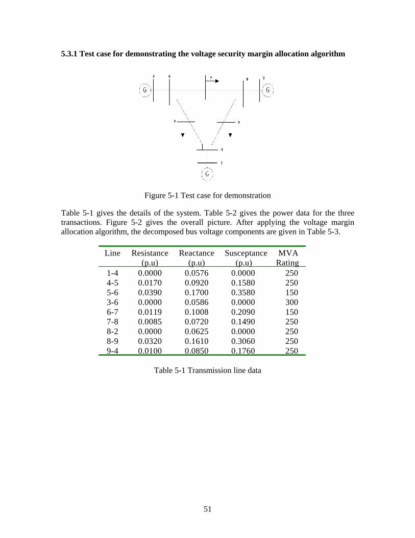
5.3.1 Test case for demonstrating the voltage security margin allocation algorithm

Figure 5-1 Test case for demonstration

Table 5-1 gives the details of the system. Table 5-2 gives the power data for the three transactions. Figure 5-2 gives the overall picture. After applying the voltage margin allocation algorithm, the decomposed bus voltage components are given in Table 5-3.

Line Resistance(p.u)

Reactance(p.u)

Susceptance MVA (p.u) Rating

1-4 0.0000 0.0576 0.0000 2504-5 0.0170 0.0920 0.1580 2505-6 0.0390 0.1700 0.3580 1503-6 0.0000 0.0586 0.0000 3006-7 0.0119 0.1008 0.2090 1507-8 0.0085 0.0720 0.1490 2508-2 0.0000 0.0625 0.0000 2508-9 0.0320 0.1610 0.3060 2509-4 0.0100 0.0850 0.1760 250

Table 5-1 Transmission line data

52

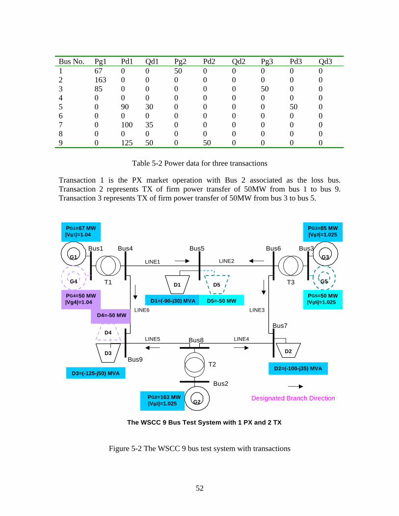
Bus No. Pg1 Pd1 Qd1 Pg2 Pd2 Qd2 Pg3 Pd3 Qd3 1 67 0 0 50 0 0 0 0 0 2 163 0 0 0 0 0 0 0 0 3 85 0 0 0 0 0 50 0 0 4 0 0 0 0 0 0 0 0 0 5 0 90 30 0 0 0 0 50 0 6 0 0 0 0 0 0 0 0 0 7 0 100 35 0 0 0 0 0 0 8 0 0 0 0 0 0 0 0 0 9 0 125 50 0 50 0 0 0 0

Table 5-2 Power data for three transactions

Transaction 1 is the PX market operation with Bus 2 associated as the loss bus. Transaction 2 represents TX of firm power transfer of 50MW from bus 1 to bus 9. Transaction 3 represents TX of firm power transfer of 50MW from bus 3 to bus 5.

Figure 5-2 The WSCC 9 bus test system with transactions

D2

Bus1

LINE1

D1

G1

G4 D5

LINE2G3

G5

D3

D4

G2

LINE5 LINE4

LINE6

Bus5

Bus7

Bus8

Bus4 Bus6 Bus3

Bus9

LINE3

Bus2

T1 T3

T2

D1=(-90-j30) MVA

D3=(-125-j50) MVAD2=(-100-j35) MVA

D5=-50 MW

D4=-50 MW

PG1=67 MW|Vg1|=1.04

PG2=163 MW|Vg2|=1.025

PG3=85 MW|Vg3|=1.025

PG4=50 MW|Vg4|=1.04

PG5=50 MW|Vg5|=1.025

The WSCC 9 Bus Test System with 1 PX and 2 TX

Designated Branch Direction

53

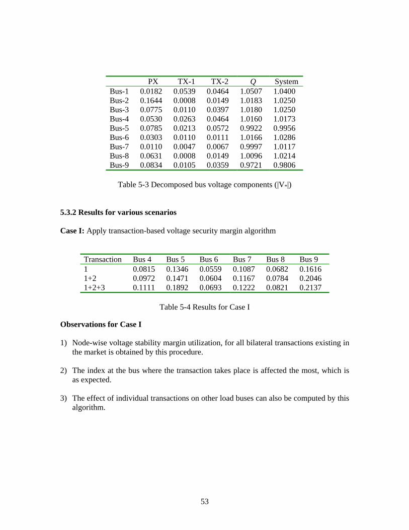
PX TX-1 TX-2 Q System Bus-1 0.0182 0.0539 0.0464 1.0507 1.0400 Bus-2 0.1644 0.0008 0.0149 1.0183 1.0250 Bus-3 0.0775 0.0110 0.0397 1.0180 1.0250 Bus-4 0.0530 0.0263 0.0464 1.0160 1.0173 Bus-5 0.0785 0.0213 0.0572 0.9922 0.9956 Bus-6 0.0303 0.0110 0.0111 1.0166 1.0286 Bus-7 0.0110 0.0047 0.0067 0.9997 1.0117 Bus-8 0.0631 0.0008 0.0149 1.0096 1.0214 Bus-9 0.0834 0.0105 0.0359 0.9721 0.9806

Table 5-3 Decomposed bus voltage components (|V*|)

5.3.2 Results for various scenarios Case I: Apply transaction-based voltage security margin algorithm

Transaction Bus 4 Bus 5 Bus 6 Bus 7 Bus 8 Bus 9 1 0.0815 0.1346 0.0559 0.1087 0.0682 0.1616 1+2 0.0972 0.1471 0.0604 0.1167 0.0784 0.2046 1+2+3 0.1111 0.1892 0.0693 0.1222 0.0821 0.2137

Table 5-4 Results for Case I

Observations for Case I 1) Node-wise voltage stability margin utilization, for all bilateral transactions existing in

the market is obtained by this procedure. 2) The index at the bus where the transaction takes place is affected the most, which is

as expected. 3) The effect of individual transactions on other load buses can also be computed by this

algorithm.

54

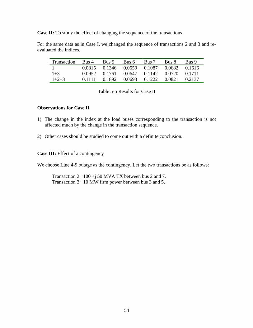
Case II: To study the effect of changing the sequence of the transactions For the same data as in Case I, we changed the sequence of transactions 2 and 3 and re-evaluated the indices.


Table 5-5 Results for Case II

Observations for Case II 1) The change in the index at the load buses corresponding to the transaction is not

affected much by the change in the transaction sequence. 2) Other cases should be studied to come out with a definite conclusion. Case III: Effect of a contingency We choose Line 4-9 outage as the contingency. Let the two transactions be as follows:

Transaction 2: 100 +j 50 MVA TX between bus 2 and 7. Transaction 3: 10 MW firm power between bus 3 and 5.

55

D2

Bus1

LINE 1

D1

G 1

D5

LINE2G 3

G 5

D3

G 2

LINE5 LINE 4

LINE6

Bus5

Bus7

Bus8

Bus4 Bus6 Bus3

Bus9

LINE3

Bus2

T1 T3

T2

D1=(-90-j30) M VA

D3=(-125-j50) M VAD2=(-100-j35) M VA

D5=-10 M W

PG 1=67 M W|Vg1|=1.04

P G 2=163 M W|Vg2|=1.025

PG 3=85 M W|Vg3|=1.025

PG 5=10 M W|Vg5|=1.025

The W SC C 9 B us Test System w ith 1 PX and 2 TX

Designated Branch D irectionP G 4=100 M W|Vg4|=1.04

D4=(-100-j50) M VA

D4

G 4

Fig 5-3 Transaction pattern for Case III


Table 5-7 Indices evaluated after the contingency


Table 5-8 Indices evaluated before contingency

Observations for Case III 1) The transaction at bus 7 has an effect on the bus 9 index, as seen in Table 5-8. 2) The above effect is magnified in the case of a contingency, also as seen from Table 5-

7. Bus 9 is driven closer to voltage collapse as the index has reached 0.8427 after transaction 2.

56

3) This seems to be because bus 9 has now lost reactive support from generator 1

following the contingency. Case IV: Study the effect of power factor of load (a) Let the transaction pattern for 2 and 3 be as follows:

Transaction 2: Firm power transfer of 50 MW from bus 1 to 9. Transaction 3: 145 + j180 MVA transfer between bus 5 and generator at bus 3.


Table 5-9 Results for case IV(a)

(b) Let the transaction pattern for 2 and 3 be as follows:

Transaction 2: Firm power transfer of 50 MW from bus 1 to 9 Transaction 3: 145 + j90 MVA transfer between bus 5 and generator at bus 3


Table 5-10 Results for Case IV(b)

Observations for Case IV 1) It can be seen from Tables 5-9 and 5-10 that the index evaluated for the same real

power transfer but with a more lagging power factor is larger, which reflects correctly the voltage stability margin sensitivity to reactive demand of load.

2) Though the load power factor is changed at bus 5, the index at load buses 7 and 9 are

affected significantly.

57

Case V: Study the location of the generator in the transactions (a) Let the transaction pattern for 2 and 3 be as follows:

Transaction 2: Firm power transfer of 50 MW from generator at bus 1 to bus 9. Transaction 3: 145 + j90 MVA transfer between bus 5 and generator at bus 1.


Table 5-11 Results for Case V(a)

(b) Let the transaction pattern for 2 and 3 be as follows:

Transaction 2: Firm power transfer of 50 MW from generator at bus 1 to bus 9. Transaction 3: 145 + j90 MVA transfer between bus 5 and generator at bus 3.


Table 5-12 Results for Case V(b)

Observation for Case V Referring to Tables 5-11 and 5-12, conducting a transaction from a nearby generator causes a smaller index. A shorter line is the reason for this. 5.4 Publications The detailed summary and application scopes of the transaction-based voltage margin allocation algorithm can be obtained from reference [5]. The formulation of the transaction-based power flow with numerical examples has been detailed in reference [10]. This new algorithm has been applied to effectively address the issue of equitable loss allocation in power markets [11]. The application scope of transaction-based power flow in formulating a congestion management policy has been detailed in reference [9].

58

One of the objectives of this project was to formulate a basis for evaluating the utilization factors and the pricing of control elements in a market-based power system, within the context of voltage stability. Using the bifurcation analysis a procedure to allocate contribution of generators, transmission and control elements in voltage stability has been evolved [6]. The authors feel that this procedure could be extended in evolving an equitable utilization factor policy for the various control elements in power system operation.

59

6 Bifurcation Analysis for Voltage Stability Margin Evaluation ________________________________________________ Thus far we have focused on the static voltage stability margin and have pointed out its potential limitations. Now we will demonstrate its limitations by looking at dynamic stability margin and find the relationships between these two margins. Our preliminary study successfully explains why the dynamic stability margin is equal or less than the steady-state stability margin; and the smaller of the two is the valid stability margin, which should be used to gauge the stability margin. Bifurcation analysis is used to calculate the dynamic stability margin, while power flow analysis is used to calculate the steady-state stability margin. Dynamic analysis is more time-consuming and difficult than steady-state analysis. For this reason, steady-state analysis has been used to estimate the stability margin. However, when the dynamic stability margin is much smaller than the steady-state margin, dynamic analysis has to be used to obtain the valid margin. Therefore, an important issue is to determine when a steady-state analysis is good enough to estimate the stability margin as shown by a simple example in section 6.2. For market-based power systems, it is important to know who contributes to avoiding a voltage collapse, where this contribution could come from different parts of the power system: generators, control systems and transmission elements, etc. Here we focus on how to allocate the responsibility and contribution by using bifurcation analysis. We investigate how parameters of the system influence the bifurcation points. Three bifurcations (that is, the singularity induced bifurcation, saddle-node and Hopf bifurcations [6]), and their relationship to several commonly used controllers, [6] are analyzed. Their parameters’ impact on the bifurcation points is investigated, from which we find a way to allocate the contribution by analyzing the relative positions of the bifurcations. There are physical limits on power system components; here we focus on deciding the size of the exciter, which has a significant influence on voltage stability. Analyzing the impacts of exciter size will benefit system design and the allocation of the responsibility of the voltage collapse in a market-based environment. The load model also has a great impact on voltage stability. We will show how different load patterns influence the bifurcation point, and thus the stability margin. In this chapter, we use a simple two-bus system shown in Figure 6-1 to demonstrate our approach. In this simple system, we assume that the voltage dynamic is decoupled from the angle dynamic, which is assumed to be well behaving, so the angle dynamic can be ignored in this scenario.

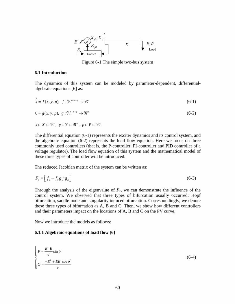
60

Figure 6-1 The simple two-bus system 6.1 Introduction The dynamics of this system can be modeled by parameter-dependent, differential-algebraic equations [6] as:

( , , ), : n m q nx f x y p f•

+ += ℜ → ℜ (6-1)

0 ( , , ), : n m q mg x y p g + += ℜ → ℜ (6-2)

, ,n m qx X y Y p P∈ ⊂ ℜ ∈ ⊂ ℜ ∈ ⊂ ℜ

The differential equation (6-1) represents the exciter dynamics and its control system, and the algebraic equation (6-2) represents the load flow equation. Here we focus on three commonly used controllers (that is, the P-controller, PI-controller and PID controller of a voltage regulator). The load flow equation of this system and the mathematical model of these three types of controller will be introduced. The reduced Jacobian matrix of the system can be written as:

1x x y y xF f f g g− = − (6-3)

Through the analysis of the eigenvalue of Fx, we can demonstrate the influence of the control system. We observed that three types of bifurcation usually occurred: Hopf bifurcation, saddle-node and singularity induced bifurcation. Correspondingly, we denote these three types of bifurcation as A, B and C. Then, we show how different controllers and their parameters impact on the locations of A, B and C on the PV curve. Now we introduce the models as follows: 6.1.1 Algebraic equations of load flow [6]

''

'

2 ' '

'

sin

cos

E EP

x

E EEQ

x

δ

δ

=

− +=

(6-4)

′dd XX ,

rEfdE

δ ′′,E δ,ELoad

X

Exciter

61

2

sin

cos

GG

G G

E EP

x

E EEQ

x

δ

δ

=

− +=

(6-5)

Equation (4) can be simplified as:

'2 2 2 2 20 ( ' ) ( ' )E E x P x Q E= − − + (6-6)

Here equation (6-6) is the g(x,y,p) in equation (6-2).

6.1.2 Differential equations of controllers The mathematic models of the three controllers are given in this section. 1) P-controller:

+

′+⋅

′−+′+

−⋅′=′•

fdddd

d

EE

QxEx

xxE

xxx

TE )'(

''1 2

0 (6-7)

0 2 2 21 1( ) ( ) ( )fd fd fd P rE E E K xP xQ E ET E

• ′ = − − − + + − (6-8)

Here equations (6-7) and (6-8) are the f(x,y,p) in equation (6-1). 2) PI-controller

2

0

1 ( ' )' '

d d dfd

d

x x x x E x QE E Ex x ET

• ′′ + − +′ = ⋅ − + ⋅ +′ ′ (6-9)

0 2 2 21 1( ) / ( ( ) ( ) )fd fd fd PI I P rE E E E T K xP xQ E ET E

• = − − − − + + − (6-10)

2 2 21( ) ( )PI rE xP xQ E E

E

•

= + + − (6-11)

Here, equations (6-9) to (6-11) are the f(x,y,p) in equation (6-1).

62

3) PID-controller For a PID controller [6],

1P D

I

K K sT s

+ + (6-12)

We know that a D-controller is not practical due to noises, so if TD is small enough, we can use equation (6-13) to replace equation (6-12):

1

1D

P

I D

K sK

T s T s+ +

+ (6-13)

Then, the control system can be expressed as below:

2

0

1 ( ' )' '

d d dfd

d

x x x x E x QE E Ex x ET

• ′′ + − +′ = ⋅ − + ⋅ +′ ′ (6-14)

0 2 2 21 1( ) / ( )( ( ) ( ) )Dfd fd fd PI I D P r

D

KE E E E T E K xP xQ E ET T E

• = − − − − − + + + −

(6-15)

2 2 21( ) ( )PI rE xP xQ E E

E

•

= + + − (6-16)

2 2 2

2

1( ( ) ( ) )D D

D r

D D

K EE xP xQ E E

T E T

•

= − + + − − (6-17)

Here equations (6-14) to (6-17) are the f(x,y,p) in equation (6-1). 6.2 Dynamic stability margin vs. static stability margin Dynamic stability margin is equal to or less than steady-state stability margin. The smaller of the two is the valid stability margin. Bifurcation analysis is used to calculate the dynamic stability margin, which is time-consuming and more difficult than steady-state analysis. If we can determine when the steady-state analysis is good enough to estimate the stability margin, we can avoid the unneeded computations. We will discuss this issue in section 6.6 based on this simple two-bus system. Here we use a simple example in reference [12] to show that the dynamic stability margin is smaller than the static margin. The regulator used in this example is a P-regulator with constant Efd0=1.6.

63

Figure 6-2 The locations of bifurcation points on PV curve

In the above figure, we found Hopf bifurcation point A in the upper part of the PV curve, which is the dynamic stability margin. We can see that PA is smaller than the static margin PB (here PB=Pmax), when the system go beyond A point, the system will lose stability after a small disturbance, as shown below.

Figure 6-3 The Dynamic Response of Two-Bus System

When the system go beyond the A point, the system has a severe oscillation and cannot maintain stability. Therefore, we know that the dynamic margin A is the stability margin, which we need bifurcation analysis to find. The static margin B point is a too optimistic estimation . 6.3 Allocate the responsibility for voltage collapse with bifurcation analysis In the following, we analyze the impacts of these controllers on the voltage stability of the system. Accordingly, we determine how to allocate the responsibility of voltage collapse. In this section, we assume constant load with a fixed power factor, and we have infinite exciter size. In all examples given in this section, we assume P=2Q.

64

6.3.1 On P-regulator We note that this P-regulator reschedules Efd0 to keep rG EE ≡ . Here we will show how Kp impacts on the locations of bifurcation points.

When Kp =2.5, 5, 10, the locations of the bifurcations A, B and C, and the eigenvalues of the reduced matrix are shown in Figures 6-4 to 6-6.

Figure 6-4 The locations of bifurcations points with Kp=2.5, 5, 10

Figure 6-5 The eigenvalue which is slightly influenced by Kp

65

Figure 6-6 The eigenvalue which is strongly associated with Kp

By our calculations, with constant load and the infinite exciter size, bifurcation point C is only determined by the transmission system. It will not be influenced by the parameters of controller. However, point B will vary when Kp changes. B approaches Pmax when KP goes to infinity. B>C when KP>5.25. B ≈ A when KP=1.895. When KP<1.895, A will disappear. B approaches 0.735 when KP approaches 0. In Figure 6-5, note that Kp has little influence on one of the eigenvalues (denoted by EigT), while in Figure 6-6, Kp has a substantial impact on the other eigenvalue (denoted by EigC). When Kp =1.8, Figure 6-9 shows the location of B and C in PV curve. A has disappeared. From Figures 6-4 to 6-9 we can see that the eigenvalue EigT is strongly related to the load flow, while the eigenvalue EigC is strongly influenced by the controller.

Figure 6-7 The curve of eigenvalue EigT when Kp=1.8

66

Figure 6-8 The curve of eigenvalue EigC when Kp=1.8

Figure 6-9 The location of B and C on PV Curve when Kp=1.8

We can conclude that there are three basic patterns:

1) PA<PB<PC. When P∈(PA,PB), both the eigenvalue EigT and EigC are positive; when

P∈(PB,PC), only the eigenvalue EigT is positive.

2) PA<PC<PB. When P∈(PA,PC), both the eigenvalue EigT and EigC are positive; when P∈(PC,PB), only the eigenvalue EigC is positive.

3) Point A disappears and PB<PC. Only the eigenvalue EigT is positive when P∈(PB,PC). 6.3.2 On PI- regulator Several important parameters are given as: Kp =2.5, TI =5.0/ TI =20. Using equation (3), (6) and (9) to (11), we can obtain three eigenvalues of the system: EigC (EigC is influenced by Kp and TI, and is mainly influenced by TI) and EigT. The other eigenvalue is always negative. We also found bifurcation points A, B and C.

67

Figure 6-10 The curve of eigenvalue EigT (PI-Controller)

Figure 6-11 The curve of eigenvalue EigC (PI-Controller)

Figure 6-12 The location of A, B and C in PV curve for PI/PID controller

From Figures 6-10 to 6-12, we can conclude that PI controller behaves very much like the P-controller case as KP ∞→ . When P∈(0,PA), all eigenvalues are negative; when P∈ (PA,PC), both eigenvalue EigC and EigT are positive; when P ∈ (PC,PB), only the eigenvalue EigC is positive. Accordingly, it follows the basic pattern 2 as described in 6.3.1.

68

6.3.3 On PID-regulator Several important parameters are given as: Kp=2.5, TI=5.0, KD=1,TD=0.01/ TD =0.005. This kind of regulator behaves like a PI-controller. This follows the basic pattern 2 as discussed in 6.3.1. Through sections 6.3.1, 6.3.2, and 6.3.3, given the constant load and infinite exciter size, we conclude that the three basic ordering patterns of bifurcation points A, B, and C (as discussed in 6.3.1) are generally true for all controllers which can keep rG EE ≡ . Our experience indicates that no other ordering of A, B, and C is possible. Accordingly, we can draw these conclusions.

1) PA<PB<PC. When P ∈ (PA,PB), both EigC and EigT are positive; and when P∈(PB,PC), only the EigT is positive. From the parameter analysis, we conclude that the voltage collapse is due to both the controller and transmission when P∈(PA,PB). The voltage collapse is only caused by the transmission part when P∈ (PB,PC). In this case, [PA, PC] is the unstable area, and PA determinesthe dynamic stability margin.

2) PA<PC<PB. When P∈ (PA,PC), both EigC and EigT are positive; and when P∈

(PC,PB), only the EigC is positive. From the parameter analysis we conclude that the voltage collapse is due to both the controller and transmission when P∈ (PA,PC). The voltage collapse is caused by the controller when P∈ (PC,PB). In this case, [PA, PB] is the unstable area, and PA determines the dynamic stability margin.

3) Point A disappears and PB<PC, only the EigT is positive when P∈ (PB,PC). Thus,

the voltage collapse is only due to transmission when P∈ (PB,PC). In this case, [PB, PC] is the unstable area, and PB is the dynamic stability margin.

4) In conclusion, the tuning of the control parameters will influence PA and PB, thus,

the dynamic stability margin of the system. This conclusion will also benefit the design of the system.

6.4 The influence of the exciter size on the bifurcation points When the exciter is at its limit, its input, Efd, will no longer be regulated with the change of the voltage. Efd will be kept as Efd_max. To demonstrate our analysis on the limit of the exciter, we draw two PV curves in Figure 6-13 and 6-14. The shorter nose curve denotes the system without regulation, which has a constant Efd = Efd_max; the longer nose curve denotes the system with regulated Efd. When the load increases, Efd will be regulated to hit its limit Efd_max at the D point (the intersection of the two PV curves), then the system will go along the PV curve with a shorter nose, which is shown by arrows in Figures 6-13 and 6-14. In this section, three widely used regulators are analyzied: P-regulator (Efd

0 is rescheduled to keep G rE E≡ ), PI-regulator and PID-regulator. Here we also assume that the load type is constant.

69

By comparing the PV curves and the locations of the bifurcation points, we found two basic patterns identified by whether the intersection point D is in upper part or lower part of the shorter nose PV curve. The two patterns are shown in Figure 6-13 and Figure 6-14 respectively: 1) Upper pattern: The intersection of two PV curves is in the upper part of the PV curve with shorter nose. In this basic pattern, the possibilities of dynamic stability margin are given as following (For each point, says D, we associate D with PD as the real load at point D.): • If PA<PD, the dynamic stability margin is PA. (If A point disappears, PB is the dynamic stability margin.). • If PA> PD, the dynamic stability margin is PB1. For steady stability margin: •If PC< PD, the steady-state margin is PC. •If PC > PD, the steady-state margin is PB1.

Figure 6-13 Upper pattern

2) Lower pattern: The intersection of two PV curves is in the lower part of the PV with shorter nose.

70

Figure 6-14 Lower pattern

In this basic pattern, the possibilities of dynamic stability margin are given as following. • If PA<PD, the dynamic stability margin is PA. (If A point disappears and PB<PD, PB is the dynamic stability margin.) • If PA>PD and PC1<PD, the dynamic stability margin is PD. • If PA>PD and PC1>=PD, the dynamic stability margin is PC1. For the steady-state stability margin, there are also several possibilities. • If PC<PD, the steady-state margin is PC. • If PC> PD and PC1< PD, the steady-state margin is PB1. • If PC > PD and PC1>= PD, the steady-state margin is PC1. In this basic pattern, PB1 can never be the dynamic stability margin. Since PC1 and PD are always less than PB1, and C1 is the singularity-induced bifurcation point, the system cannot go beyond point C1. But when PC> PD and PC1< PD, with load perturbation analysis, we know that the system can go beyond point D and will go to point B1, so PB1 is the steady-state margin. According to our experience, the scenario PC > PD seldom occurs. In our study, it appears with a short transmission line, one that is less than 50 miles long. Comparing Figure 6-13 to Figure 6-14 shows that xd and Efd_max in Figure 6-14 are larger than those in Figure 6-13, and the point D in Figure 6-14 is nearly at the same position as point B1 in Figure 6-13. This implies that larger exciter size is required for bigger xd to keep same voltage stability margin for a given transmission line. Also, larger exciter size is required for longer transmission lines to keep same voltage stability margin for a given xd. Based on our analysis in section 6.3, we conclude that the situation PA(PB) <PD only occurs when the regulator is not well tuned (e.g., Kp is too small), or the transmission line is too long. In this case, dynamic analysis is necessary, and point A is the real stability margin because that PA is always less than PC. It is known that point A is mainly caused

71

by the regulator for a given transmission line, so the regulator is mainly responsible for the voltage collapse in this case. Steady-state analysis is no longer good enough in this case, as the real stability margin is determined by point A. According to our experiences, situations PA>PD, PC>PD and PC1<PD are found in most cases (with a well-tuned regulator and transmission lines that are not too long). PD is usually the real stability margin for the lower pattern, while PB1 is the real stability margin for the upper pattern. Both PB1 and PD can be solved by the steady-state method. For these cases, steady-state analysis is good enough. Given a transmission line, PD and PB1 are mainly determined by the exciter size; thus, the exciter should be mainly charged for the voltage collapse in this case. 6.5 The influence of the load pattern on the bifurcation points In Chapter 1, we analyzed the influence of load pattern. Here we extend the study to bifurcation analysis, and show how different load patterns influence the PV curve and bifurcation points. From Chapter 1, we know the load model can be expressed as:

P = P0 (E/E0)PE * ( 0/ωω )Pf

Q = Q0 (E/E0)QE *( 0/ωω )Qf

000 PQ β=

Here we still assume that the voltage dynamic is decoupled from the angle dynamic, which is well behaved, so the angle dynamic can be ignored. Thus, in our analysis, we can assume that 1/ 0 ≡ωω . Now we will discuss how PE, QE and β impact voltage stability.

72

6.5.1 The influence of 0β

Figure 6-15 The influence of 0β

In Figure 6-15, there are three PV curves in which all load pattern are constant load,

0β equals to 0.5, 0 and –0.5 respectively; the other conditions are kept as same. We see that 0β has a big influence on the dynamic and static stability margins, and we have a bigger Pmax and stability margin with smaller 0β . 6.5.2 The influence of PE and QE on Pmax

We define PEQEPE

QE

EEPEQ

PQ −=== 0

0

0 ββ ; it corresponds to the power factor of the load.

When 0β =0, it is apparent that β = 0β , PE and QE will have no influence on the Pmax. When 0β >0,

If QE>PE, PEQEE − <1, so β < 0β , we have bigger Pmax than constant load; If QE<PE, PEQEE − >1, so β > 0β , we have smaller Pmax than constant load; and If QE=PE, PEQEE − =1, so β = 0β , we have the same Pmax as constant load.

When 0β <0,

If QE>PE, PEQEE − <1, so β > 0β , we have smaller Pmax than constant load;

73

If QE<PE, PEQEE − >1, so β < 0β , we have bigger Pmax than constant load; and If QE=PE, PEQEE − =1, so β = 0β , we have the same Pmax as constant load.

Example:

Figure 6-16 Bifurcation point locations on PV curve

with load parameters 0β =0.5, PE=0, and QE=0


with load parameters 0β =0.5, PE=-2, and QE=0

74


with load parameters 0β =0.5, PE=0, and QE=-2


with load parameters 0β =0.5, PE=2, and QE=2 Comparing Figures 6-16 and 6-17, we see that when 0β >0, and QE>PE, we have bigger Pmax than constant load. Comparing Figures 6-16 and 6-18, we see that when 0β >0, and QE<PE, we have smaller Pmax than constant load. Comparing Figures 6-16 and 6-19, we see that when 0β >0, and QE=PE, we have the same Pmax as constant load. 6.5.3 The influence of PE and QE on bifurcation points 6.5.3.1 The influence of PE and QE on singular point C For the described load above, there is no singular point C when 00 =β and 1≥PE . This can be easily derived from the following equations.

75

g: '2 2 2 2 20 ( ' ) ( ' )E E x P x Q E= − − + , (6-18)

00000 , , PQEQQEPP QEPE β=== (6-19)

Examples:

Figure 6-20 No bifurcation point locations on PV curve with lighting load

Figure 6-21 Bifurcation point locations on PV curve with constant load

Comparing Figure 6-20 to Figure 6-21, we see that there is no singular point when 0β =0 and 1≥PE , but when 0β =0 and 1<PE , singular point C will appear.

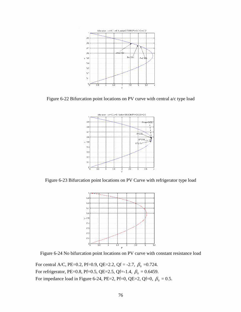
76

Figure 6-22 Bifurcation point locations on PV curve with central a/c type load

Figure 6-23 Bifurcation point locations on PV Curve with refrigerator type load

Figure 6-24 No bifurcation point locations on PV curve with constant resistance load

For central A/C, PE=0.2, Pf=0.9, QE=2.2, Qf = -2.7, 0β =0.724. For refrigerator, PE=0.8, Pf=0.5, QE=2.5, Qf=-1.4, 0β = 0.6459. For impedance load in Figure 6-24, PE=2, Pf=0, QE=2, Qf=0, 0β = 0.5.

77

6.5.3.2 The influence of PE and QE on other bifurcation points Based on our observation on the simple two-bus system, we found that with bigger PE, A, B and C points go further down to Pmax. Therefore, we have a larger stability margin. When 0β >0, with larger QE, A, B and C points go further down to Pmax, so we can have a larger stability margin. However, when 0β <0, with smaller QE, A, B and C points go further down to Pmax, which also means that we have a larger stability margin. It is apparent that QE will have no influence when 0β =0. Examples: Comparing Figure 6-16 to Figure 6-17, we see that with a larger PE in Figure 6-16, there is a larger stability margin than in Figure 6-17. Comparing Figure 6-16 to Figure 6-18, we see that when 0β >0, with a bigger QE in Figure 6-16, there is a larger stability margin than in Figure 6-18. 6.6 Publications For the allocation of the responsibility/ contribution of the voltage stability, reader can refer to the paper in reference [6].

78

7 Conclusions ________________________________________________ The phenomenon of voltage stability within the context of an increasingly competitive power market environment has been explored in this project. The effects of FACTS devices and types of load on voltage stability limits have been analyzed. Modeling issues for studying the effects of the various components have been discussed. A voltage stability indicator has been analyzed to represent the phenomenon during a variety of control situations. The numerical simulation demonstrated the indicator’s applicability. The proposed voltage stability indicator has been explored for its applicability to detect a potential dynamic voltage collapse situation. Results from time-domain simulations using EUROSTAG, a commercial software product, has been used to compute the indicator. The importance of dynamic generation reserves on dynamic voltage stability has also been studied through time-domain simulations in this project. [8] An algorithm to incorporate steady-state voltage stability into conventional optimal power flow formulation has been proposed. Incorporating FACTS devices and its application in composite reliability analysis was studied. A transaction-based power flow procedure has been developed to effectively address the issue of equitable loss allocation and congestion management in a market environment. A new procedure to allocate voltage stability usage on a transaction basis has been proposed. We feel that this procedure has the potential to address utilization, responsibility settlement, security management and pricing from the voltage stability perspective. Finally, a new way of using bifurcation analysis to allocate the contribution of generators, transmission and control elements has been proposed. The impacts of load patterns and exciter sizes on dynamic stability were also discussed. These analyses can help in allocating responsibility for a stability problem, and can also be of benefit in designing the system to avoid voltage collapse.

79

References ________________________________________________

[1] G M Huang, N C Nair, “An OPF based Algorithm to Evaluate Load Curtailment Incorporating Voltage Stability Margin Criterion”, Conference proceeding of NAPS 2001, TX.

[2] G M Huang, N C Nair, “Voltage Stability Constrained Load Curtailment Procedure to Evaluate Power System Reliability Measures”, IEEE/PES WM 2002, NY.

[3] G M Huang, N C Nair, ”Incorporating TCSC into the Voltage Stability Constrained OPF Formulation”, IEEE/PES Summer meeting 2002, Chicago.

[4] G M Huang, N C Nair, “Detection of Dynamic Voltage Collapse”, IEEE/PES Summer meeting 2002, Chicago.

[5] G M Huang, N C Nair, “Allocating Usages of Voltage Security Margin in Deregulated Electric Markets”, ISCAS 2003, Thailand.

[6] G M Huang, K Men,” Contribution Allocation for Voltage Stability in Deregulated Power Systems”, IEEE 2002 PES, Summer meeting, Chicago.

[7] G M Huang, L Zhao, X Song, “A new bifurcation analysis for power system dynamic voltage stability studies”, IEEE 2002 PES, Summer Meeting, Chicago.

[8] G M Huang, H Zhang, “Dynamic voltage stability reserve studies for deregulated environment” IEEE 2001 PES, Summer Meeting, Canada

[9] G M Huang, H Zhang, “Transaction-Based Power Flow Analysis for Congestion Management and Responsibility Evaluation” presented at 2001 IEEE/PES Winter Meeting, Panel Session: Transmission Congestion Management and Reliability, Columbus, Ohio.

[10] G M Huang, H Zhang, “Transaction-based Power Flow analysis For Transmission Utilization Allocation”, 2001 IEEE/PES Summer Meeting.

[11] G M Huang, H Zhang, “Transmission Loss Allocations and Pricing Via Bilateral Energy Transactions”, 1999 IEEE/PES Summer Meeting., Chicago, IL.

[12] V Venkatasubramanian, H Schaettler and J Zaborazky, "Voltage Dynamics: Study of a Generator with Voltage Control, Transmission, and Matched MW Load", IEEE Transactions on Automatic Control, Vol. 37, No.11, November 1992, pp. 1717-1733.

[13] Carson W Taylor, “Power System Voltage Stability”, McGraw-Hill, Inc., 1994.

[14] P Kessel, H Glavitsch, “Estimating the voltage stability of a power system”, IEEE Transactions on Power Delivery, Vol. PWRD-1, No.3, July 1986, pp. 346-354.

voltage security margin assessment · voltage security margin assessment ... the industry advisors...

Documents