volume 1, number 4, july 1979 - semantic scholar...bulletin (new series) of the american...

BULLETIN (New Series) OF THE AMERICAN MATHEMATICAL SOCIETY Volume 1, Number 4, July 1979

COMPLEX ANALYSIS AND ALGEBRAIC GEOMETRY

BY PHILLIP A. GRIFFITHS1

The theme of these four lectures is roughly "the history of, and some recent developments in, the study of algebraic geometry by analytic methods". Since this topic is much too broad I have chosen to isolate one particular analytic tool, the local notion of residue and subsequent global residue theorem, and will attempt to illustrate some ways in which residues may be used in both classical and modern problems in algebraic geometry.

The first lecture begins with the definition and basic local and global properties of the point residue in several variables. Next, both as an application of one of these local properties and for use in the third lecture, we derive some theorems of Macaulay from the classical theory of polynomial ideals. Finally we discuss the global residue theorem for the projective plane, where it will turn out to pertain to the possible configurations of points arising as the intersection of two algebraic plane curves. The simpliest special case here is the Pascal theorem, with which we conclude the lecture.

In the second talk we begin by deducing the classical form (which is in many ways more flexible than the modern version) of Abel's theorem, also from the global residue theorem for P2. This result is then applied to the inversion of the elliptic integral, with which much of modern algebraic geometry began and with which, at least on the number-theoretic side, it is still concerned with. Next we turn to two topics from elementary geometry. The first is the theorem of Poncelet which is given as an application of the elliptic integral, and the second is a recreational result shown to me by Joe Harris and Dave Morrison giving a geometric property of the cardioid as an application of Abel's theorem for singular curves.

Now I said previously that the motif of these lectures was to be "residues", but from here on this should probably be amended to read "residues and Hodge theory". With this in mind the second lecture represents the beginnings of our new main theme, one which will now to some extent be formalized both for curves and for higher-dimensional varieties. Following a recollection of the highlights of the relationship between an algebraic curve and its Jacobian we give a very brief sketch of some aspects of Hodge theory for general varieties. Then we turn to smooth hypersurfaces in projective space where the relation between Hodge theory and residues turns out to be quite direct. For example, using Macaulay's theorem from the first lecture it

A series of four Colloquium Lectures presented by Phillip A. Griffiths at Biloxi, Mississippi, January 24-27, 1979; received by the editors October 30, 1978.

AMS (MOS) subject classifications (1970). Primary 32J25. Research partially supported by NSF Grant MCS-78-07348.

© 1979 American Mathematical Society 0002-9904/79 /0000-0300/$09.00

595

596 P. A. GRIFFITHS

is shown that the Hodge structure on the cohomology locally determines the hypersurface up to a projective transformation.

Finally, in the fourth lecture we specialize to cubic hypersurfaces. Here the interplay between the Hodge theory and the projective geometry has in the second lecture been explored for cubic curves, and for cubic surfaces it essentially amounts to the famous configuration of 27 lines. Turning to the cubic threefold F c P 4 the Hodge theory amounts to the intermediate Jacobian, the projective geometry has to do with the Fano surface S of lines on V, and the relation between these may be expressed by interpreting, via the Abel-Jacobi map, the differentials on S as residues of differentials on P4

having a double pole along V. Our point here is to explain how analytic considerations centered around Hodge theory and residues enter into contemporary as well as classical problems in geometry, and it is with this discussion that these lectures conclude.

A list of the references for the individual talks appears at the end of all four of the lectures.

I. Residues and elementary applications. (a) Local properties of residues and the residue theorem. We begin by

discussing the definition and local properties of residues. The notation 0 for the local ring of complex analytic functions f(z) defined in some neighborhood U (depending on ƒ) of the origin in Cn will be used; 0 is just the convergent power series in z„ . . . , zn. The locus {z G U: f(z) = 0}, suitably counted with multiplicities, defines the divisor D of/. In one variable D is just the origin counted with multiplicity, while f or n = 2 we may picture D as a piece of analytic curve generally having a singularity at the origin; e.g., Figure 1 gives the real points of the cusp.

FIGURE 1

Given n analytic functions fl9 . . . , ƒ , E 0 having respective divisors Dl9..., Dn with the origin as isolated intersection, e.g. Figure 2, for any g E 0 we set

_ g(z)dz{ A • • • /\dzn

/ i (*)- - 'A(*)

COMPLEX ANALYSIS AND ALGEBRAIC GEOMETRY 597

and define the residue by

ReS{o) w={ krïfc' (u)

where the cycle of integration T - [z: \f,(z)\-8,}

is oriented by rf(arg fx) A • • • Ad(arg fn) > 0. Although this definition has been around since the early days of several complex variables its deeper properties emerged only recently in connection with Grothendieck's general duality theory, and for this reason (1.1) is generally referred to as the Grothendieck residue symbol.

FIGURE 2

The residue symbol has elementary properties familiar from one variable, such as invariance under deformation of the path r in U — D where D = Dx u • • • U Dn is the polar locus of co. Also Res{0} co is clearly linear in g but is alternating in f l 9 . . . , fn due to the orientation of T. One property not so visible in the classical case is that there is canonically associated to co a closed differential form TJW of degree 2/i — 1, which is C00 in U - {0} but has a point singularity at the origin, and which satisfies

Res{0} co = f 7jw. (1.2) •1*11-*

Of course, r?w = co when n = 1, but when n > 2 it is necessary to leave the class of meromorphic forms in order to express (1.1) as an integral over a small sphere around the origin. Setting/(z) = (fx(z),... >fn(z)) viewed as a holomorphic mapping ƒ : ( / - > C1, in the generic case when the Jacobian determinant

y/°)=iyi""'fn\(o)*o, o(z„ . . . , zn)

598 P. A. GRIFFITHS

which is equivalent to saying that the Dt are smooth and meet transversely, we may make the change of variables w, = ƒ (z) to write

g{w) dwx dwn

and evaluate (1.1) by iterating Cauchy's formula obtaining

Res{0)W = A . (1.3)

Our discussion of further properties will be facilitated by introducing the ideal ƒƒ={ƒ„ . . . ,ƒ„} c 0 generated by the ft{z). If g(z) E If; e.g., if g = hfl9 then

^ h(z)dzy A • • • Adzn

and the path T may, without crossing a singularity, be shrunk to a lower dimensional cycle by letting ô1 -^ 0. Thus

Res{O}<o = 0 iîgelp (1.4)

and so we may define a pairing

Res/ 0 / 7 ® C 0 / / ^ C (1.5)

by setting

Res (e to -Res *&*&** A ' ' ' A<fe" Res/g, *) - Re»{0) fl(z). . . fn{z) •

Our last two local results give the basic properties of this pairing. For the first suppose that we have relations

J

where the divisors D[ also have the origin as isolated common intersection; algebraically this means that If c If. Then, setting

A(z) - det(^(z))

the transformation formula

g(z)dz1 A • • • f\dzn _ à(z)g(z)dz1 A • • • /\dzn 5{0) ƒ , ( * ) • • - A W " {0} / Ï W - - - J 2 W

is valid. When everything is nondegenerate (1.6) follows from (1.3). The general case is reduced to this one by using a perturbation to break the degenerate zero into a finite number of nondegenerate ones and writing the original residue as the limit of a sum of residues at nondegenerate zeroes. The second property is the

(1.7) LOCAL DUALITY THEOREM: The pairing (1.5) is nondegenerate.

This is proved in the following way: In case ƒ (z) = zp the question may effectively be reduced to one variable by iterating the residue integral. In


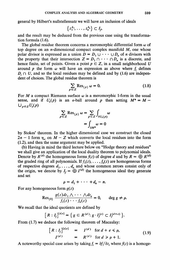
general by Hilbert's nullstellensatz we will have an inclusion of ideals

{zxk •, . . . , z£}clp

and the result may be deduced from the previous case using the transformation formula (1.6).

The global residue theorem concerns a meromorphic differential form <o of top degree on an «-dimensional compact complex manifold M, one whose polar divisor is expressed as a union D = Dx u • • • U Dn of n divisors with the property that their intersection Z = Dx n • • • H Dn is a discrete, and hence finite, set of points. Given a point p E Z, in a small neighborhood U around p the form to will have an expression as above where fê defines Dt n U, and so the local residues may be defined and by (1.6) are independent of choices. The global residue theorem is

2 Res{/,} co = 0. (1.8)

For M a compact Riemann surface (o is a meromorphic 1-form in the usual sense, and if Ue(p) is an c-ball around p then setting M* = M — U,6 2£/.Q»

S Res{W o>= *2 [ co

= f (0 = 0

by Stokes' theorem. In the higher dimensional case we construct the closed 2n — 1 form rjw on M — Z which converts the local residues into the form (1.2), and then the same argument may be applied.

(b) Having in mind the third lecture below on "Hodge theory and residues" we shall give an application of the local duality theorem to polynomial ideals. Denote by R(d) the homogeneous forms/(z) of degree d and by R = 0 R(d)

the graded ring of all polynomials. Iffx(z)9..., fn(z) are homogeneous forms of respective degrees dl9..., dn and whose common zeroes consist only of the origin, we denote by If = © I{d) the homogeneous ideal they generate and set

p = dx + • • • +dn — n.

For any homogeneous form g(z)

g(z)dzx A • • * /\dzn

We recall that the ideal quotients are defined by

[ R : If]ld'e] = { g G R « >: g • ƒ/«> C l}d+e) }.

From (1.7) we deduce the following theorem of Macaulay:

[ * : / ƒ ] " " = ƒ<"> f o r < / + e < p ,

/«O = flOO ford>p+l.

A noteworthy special case arises by taking^ = 3//6z( where/(z) is a homoge-

Res{0} ,,_[ t ,_^ " = 0, deg g ¥= p.

600 P. A. GRIFFITHS

neous form. The condition that the divisors Di intersect only in the origin is equivalent to the nonsingularity of the hypersurface in Pn_, defined by f(z). In this example If is called the Jacobian ideal of the homogeneous form/, and in the third lecture (1.9) will be applied to study its properties. There we shall also need the following: If we have a relation

2&/Î-0

where the gt are homogeneous forms of degree et with et + dt = d for all /, then

& = 2 ^ fy + fy = o, (l.io)

where the htj are homogeneous forms of degree ei — dr We may prove (1.10) from (1.7) as follows: Setting Ü = dzx A • • • /\dzn, for any form h

Res &*Q - Res &fi*° K e S ( 0 } f . . . f ~ K e S { 0 } T x2 *

by applying (1.4) to the ideal {ƒ„ . . . , ft,..., ƒ„}. It follows from (1.9) that g, G /ƒ. Writing

Si = 2 *ÖÜ&.

we may similarly conclude that htj + h}i E / . An induction argument then gives that

hv + hJê = 2 M

where ^ = kjV = - A -. Then we may modify htj to have hi} + A,, = 0. (c) Even the simplest special cases of the global residue theorem (1.8) are

interesting. For example, suppose that M = P„ is a complex projective space with affine coordinates (x{9 . . . , xn) on Cn c Pw. The divisor Dt will be given in C" by the zeroes of a polynomial ji(x) of some degree di9 and consequently the meromorphic n-ïorm co has on Cn an expression

_ g{x)dxx A * ' * /\dxn

where g(x) is a polynomial. To determine its degree d we set 1 x2 x„

A l A I A l

a = (rfj + • • • + <<,)-(» + 1),

and then

gOO^i A • • • A4v„ to =

^ . W - - ' / . W


where

It follows that

g{x)dxx A ' • • /\dxn (1.11)

rf< (rfi + • • • +</„) - ( « + 1)

gives the most general such meromorphic H-form on P„. Suppose now we assume that the points of intersection of Dl9..., Dn are

distinct points in Cn. Writing this intersection additively in the form

Dr-Dn = Z =ƒ>! + • • • +p8

where 8 = dx • • • dn by Bezout's theorem, from (1.3) and (1.8) we deduce the formula due to Jacobi

where

2 777T = o (1.12) v Jf\Pv)

*^W 3(x„...,x„) (x )-

When /Î = 1 this is the Lagrange interpolation formula

f(P,)=o f(p„) = 0, degg(x) < deg/(x) - 2,

and it was in this context that Jacobi was led to the general result. When n = 2 we are in the projective plane. It is convenient to change

notations slightly and use (x, y) for coordinates and write the polar divisor of <o as C + D where C and D are plane curves f(x, y) = 0 and g(jc, .y) = 0 of respective degrees m and w. The Jacobi relation (1.12) is

I.*(*)/(î£îH-* *»* <m + H - 3 , (1.13)

and this immediately implies the theorem of Cayley-Bacharach:

(I A4) If E is a plane curve of degree m + n — 3 passing through all but one point of C n D, then it passes through the remaining point also.

We may interpret this result as imposing conditions on configurations of points in the plane to be the common zeroes of a pair of polynomials, conditions which turn out in general to be sufficient. When m = n = 3 all three curves are cubics, and then a special case of (1.14) is

PASCAL'S THEOREM. The opposite sides of a hexagon inscribed in a conic meet in 3 colinear points.

602 P. A. GRIFFITHS

PROOF. If we label the conic as Q, the sides as Lv ..., L6 and set py = Lt n Lp then in (1.14) we may take

C^L, + L3 + L5,

D = L2 + L4 + L69

E = 6 + PltflS

to conclude that the lint pup25 passes through p36.

FIGURE 3

For the converse to Pascal's theorem, we take the hexagon C + D as above and let g be a conic through any 5 of the 6 vertices. Then if p36 is on the line Pi4p25> we conclude that Q must pass through the remaining vertex.

II. Residues and Abel's theorem, (a) We begin by deriving Abel's theorem for plane curves from the residue theorem. An algebraic plane curve is given in C2 by a polynomial equation

/(*>>0 = 0. (2.1)

As usual we add the points at infinity, and so consider C as a compact analytic subvariety of the projective plane P2. If deg ƒ = n then C meets the infinite line in n points. For example, for the plane cubic

y2-p(x)-o (2.2)

where p(x) = (JC - xx)(x - x2)(x - x3), JC, distinct if we set x = x'/y' and

y = 1/y, then from

y2 -P(x) - (y) (y2 " (*' - *'*i)(*' - / * * ) ( * ' - / * 3 »

we conclude that C meets the line y' = 0 at the point x' = 0 counted three times. Consequently the infinite line is a flex-tangent to the complete curve as depicted by the behaviour as x -» oo in the graph of its real points:


e FIGURE 4

This particular curve is smooth, but in general we shall allow C to be singular or reducible but it should have no multiple components.

If we label the roots of the equation f(x, y) = 0 asyx(x)9... 9yn(x), then the yt(x) are algebraic functions of x on the punctured x-sphere. By the well-known procedure of analytic continuation plus careful attention to the branch points we may construct the abstract Riemann surface C associated to this algebraic function. C may be viewed as a compact complex manifold together with a holomorphic mapping C -* P2, whose image in C and which is one-to-one away from its singularities. For the cubic curve (2.2), C = C is the Riemann surface of the algebraic function Vp(x) > and is therefore represented as a 2-sheeted covering of P, with branch points at x„ x2, x3, oo.

Before discussing abelian differentials we want to explain the notion of residues along higher dimensional subvarieties. Let M be a complex manifold and V c M a complex analytic hypersurface. If Vs c F is the set of singular points, then V* = V — Vs is a complex submanifold of M * = M — Vs. Given a metric on Af, over any compact subset of F* (i.e., away from the singularities) the normal bundle to V* in M* may be identified with the tubular neighborhood Ne of radius e. For any chain y in F* we denote by r£(y) that part of dNe lying over y, so that T£(y) may be thought of as a family of e-circles in M — V* parametrized by y. If dim M = m, y is a chain of real dimension m — 1, and w is a meromorphic m-form on M with poles on V9

then by a residue integral we mean one of the form

lim — = - f o. (2.3) e-*0 2?rV ~ 1 Jre(y)

Of course this limit will not always exist. If y is a cycle in Hm_x(V*9 Z), then r£(y) will be a cycle in Hm{M — V, Z) and by Stokes' theorem the integral in (2.3) is independent of e. The limit also exists when <o has a first order pole along V, and this brings us to the notion of the Poincaré residue.

P. A. GRIFFITHS

FIGURE 5

Locally, any co with a first order pole along V has an expression

g(x)dzl A • • • /\dzm co =

A*) where/(z) = 0 is a local defining equation for V. Noting that ^J^f/^z^dz^y = 0 we infer that

Res co (-l)-,g(z)dzlA-- Adz, A Adz„

m*)/**, (2.4)

is independent of /, and this is the Poincaré residue. Since the singular locus Vs is defined by ƒ = df/dzn = • • • = df/dzm = 0, Res co is holomorphic in y* = v — Vs and by iterating the usual 1-variable residue theorem

lim -• - * 2TTV

, j co = /Res co. - 1 Jr*{y) Jy

(2.5)

Returning to our algebraic plane curve, as noted in (1.11) the meromorphic 2-forms on P2 having simple poles along C are

<p = p(x,y)dx /\dy

deg/? < n — 3,

and the Poincaré residue of <p is

= p(x,y)dx

Sy{x>y) (2.6)

restricted to ƒ = 0. The forms (2.6) are the abelian differentials on the curve. For any/7 e C* their indefinite integrals

u(p) = (Po) (2.7)


are defined up to periods, and are thus multi-valued holomorphic functions called abelian integrals. For example, the abelian differential on the curve (2.2) is co — dx/y, and using the Riemann surface representation of this curve the abelian integral (2.7) is the classical elliptic integral

dx (2.8) / VJ(x)

It is with their study that much of transcendental algebraic geometry began. The elliptic integral (2.8) is not expressible in terms of elementary functions

(in contrast to fdx/vl — x2 ), and its understanding caused considerable difficulty. The point turns out to be that one should not just consider the single indefinite integral (2.7), but should consider general abelian sums

/ - 2 u(p,) = 2 ƒ*» Po

Certain of these turn out to obey easily expressed laws or addition theorems; this is the content of Abel's theorem which we now explain.

Suppose that g(x, y, i) is a family of polynomials of degree m whose coefficients depend holomorphically on a parameter t. Each g(x, y91) defines a plane curve Dr and we think of the intersection

as being a set of points varying with t (certain of the points of C n Dt will be fixed and the others variable). Then we have

ABEL'S THEOREM. The abelian sum

/ ( 0 - 2 f ° « (2-9)

is constant modulo periods.

PROOF. We writept(t) = (xf-(0> ^/(O) a n ( i <° = pdx/fy Then by calculus

ÉL = v /K*/(0>.r/(0)*;(0 n i nv

Differentiation of the equations

f(xi(t),yi(t)) = 0,

g(xi(t),yi(t),t) = 0

gives

gxx'i + gyy'i + g, = 0,

and solving these equations we obtain at/>,•(*)

fy 8,/Hx,y)-

606 P. A. GRIFFITHS

Plugging this into (2.10) yields

f = 2/»(w,)&(w*)/ $£§(wi) = o by the Jacobi relation (1.12).

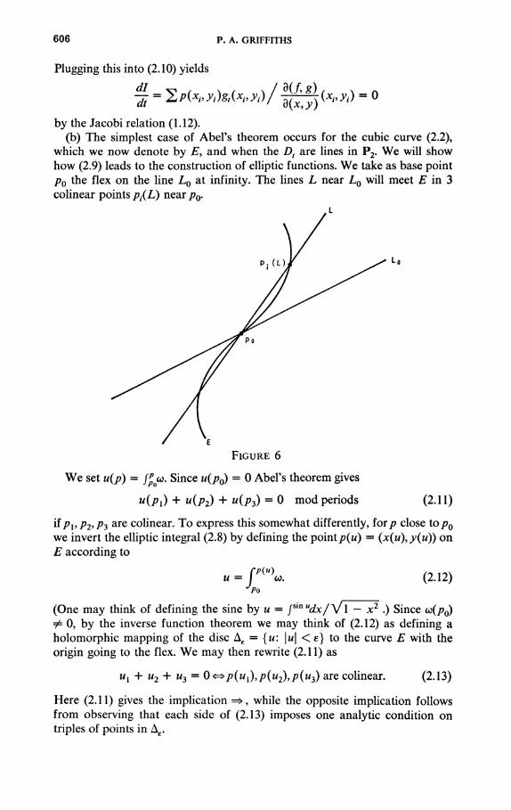
(b) The simplest case of Abel's theorem occurs for the cubic curve (2.2), which we now denote by E, and when the Dt are lines in P2. We will show how (2.9) leads to the construction of elliptic functions. We take as base point p0 the flex on the line L0 at infinity. The lines L near L0 will meet £ in 3 colinear points pt{L) near/?0.

FIGURE 6

We set u(p) = /£o<o. Since u(p0) = 0 Abel's theorem gives

u(px) + u(p2) + ti(p3) = 0 mod periods (2.11)

if pi,p2,P3 are colinear. To express this somewhat differently, for/? close top0

we invert the elliptic integral (2.8) by defining the point p(u) = (x(u),y(u)) on E according to

P(u) /~ ^ x

co. (2.12) JPo

(One may think of defining the sine by u = /^"Vfa/Vl - x2 .) Since <4p0) =£ 0, by the inverse function theorem we may think of (2.12) as defining a holomorphic mapping of the disc Ae = {u: \u\ < e] to the curve E with the origin going to the flex. We may then rewrite (2.11) as

ux + u2 + u3 = 0 <=»/?(Mi)>P(U2)>P(U3) a r e colinear. (2.13)

Here (2.11) gives the implication =>, while the opposite implication follows from observing that each side of (2.13) imposes one analytic condition on triples of points in Ae.


Now we come to the punch line. Given ux and u2, the coordinates of the third point of intersection of the line p(ux)p(u2) with E are clearly rational functions of the coordinates of p(ux) and p(u2). Using (2.13) we may express this as

x(~ (ux + u2)) = R(x(ux),y(ux), x(u2),y(u2)),

y{- (ux + u2)) = S(x(ux),y(ux), x(u2),y(u2))

where R(xx,yx, x2,y2) and S(xx,yx, x2,y2) are rational functions of their arguments. Taking u = ux = u2 we obtain the duplication formula

x( — 2u) = R(x(u),y(u)),

y{-2u) = S(x(u), y(u)%

a functional equation which allows us to extend the domain of x{u) and >>(w) to A2e. Continuing in this way we obtain entire meromorphic functions such that the curve E is given parametrically by

u -> (x(u), y(u)), u<EC. (2.14)

In fact, x(u) is essentially the Weierstrass/?-function, and from

, dx(u) x'(u) , du = —f-f = —f-f du y(u) y(u)

we see that y(u) = x'(u). The algebraic relation y2 = p{x) defining E is the famous differential equation satisfied by the Weierstrass functions. What we have essentially done is to give the classical proof, based on the addition theorem (2.11) for the elliptic integral, that any smooth cubic curve is uniformized by elliptic functions. Henceforth we shall write the map (2.14) in the more modern form as giving a biholomorphism

E = C/A9 (2.15)

where C is the universal covering of the Riemann surface E, A is the period lattice of the elliptic integral (2.8), and where the explicit map has been accomplished by using the addition theorem in the form (2.13).

(c) One of the early applications of elliptic functions to elementary geometry was to the theorem of Poncelet. This concerns a pair of conies C and Z>, and asks when the construction

(/»,9-(/>',8-(/>',r) (2-16)

depicted in Figure 7 leads to a closed polygon of (say) n sides which is both inscribed in C and circumscribed about Z>. The result is

PONCELET'S THEOREM. The construction (2.16) leads to a closed n-sided figure for one choice of initial data (p, £) <=> this is true for any choice of initial data.

608 P. A. GRIFFITHS

FIGURE 7

We shall now give a proof of Poncelet's theorem, one which can be pursued a little further to give the explicit condition for the the existence of such a closed rt-gon.

For the proof we denote by P£ the dual projective space of lines £ in P2

and by D* c P * the dual curve of tangent lines to D. The basic object underlying the construction (2.16) is the incidence correspondence E c C X D* defined by

E={(p,Ç):pt£}.

To obtain some understanding of E we recall that by stereographic projection any conic is rationally parametrized by the 1-1 map t->p(i) = (x(t),y(t)) depicted in Figure 8. Moreover, since through any point outside D there clearly pass exactly two tangent lines to this conic it follows that D* is a plane curve of degree 2, and hence a conic. The mapping E -» D* given by (/*> £) —» £ realizes £ a s a 2-sheeted covering over the Riemann /-sphere. The branch points occur over the lines £ which are tangent to both D and C; these bitangents are the four points of intersection of C* and D* in P£.

Po

( t )

t Pi

FIGURE 8


FIGURE 9

Taking one of these to be the point t = oo, and calling the others tx, t2, t3

and setting q(i) = (t — t^)(t — t2)(t — t3), we have realized E as the Riemann surface of the algebraic function V # ( 0 or equivalently, as the algebraic plane curve s2 — q(t) = 0. Consequently, E is an elliptic curve and by inversion of the elliptic integral has the form (2.15).

Now on E there are a pair of involutions /, i' given by

i(P, 8 = (p', 0, i'(p', i) = (P', r)

in Figure 7. The Poncelet construction (2.16) is the composition y = i' • /, and it is clear that iterating this construction n times gives a closed «-gon if, and only if,

Jn(P, 0 - (P, O- (2-17) On the universal covering C of E as given by (2.15) any involution lifts to an automorphism of C, which must have the form

u-> ±u + v, « E C . The minus sign occurs when the involution has fixed points, and this is the case for both / and /'. Consequently the lifting./ of j has the form

j(u) = u + w.

Denoting by u0 a point lying over (/?, £) we deduce that:

jn(p, 0 = (p91) <*jnuQ = u0 mod A

<=*> nw = 0 mod A. This last condition is independent of u0, which proves Poncelet's theorem.

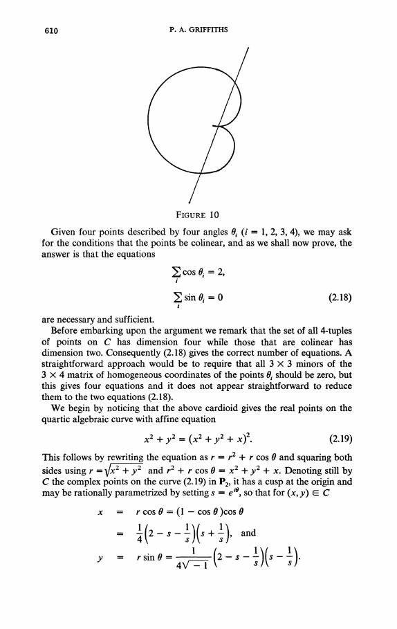
(d) Abel's theorem is customarily given only for smooth algebraic curves or equivalently for compact Riemann surfaces. However, (2.9) is valid more generally, and indeed many of the nicest applications to elementary geometry arise by taking singular and/or reducible curves. As an illustration of this we shall discuss the cardioid, which we recall is the curve C with polar coordinate equation r = 1 — cos 0 and graph

610 P. A. GRIFFITHS

FIGURE 10

Given four points described by four angles 0, (i = 1, 2, 3, 4), we may ask for the conditions that the points be colinear, and as we shall now prove, the answer is that the equations

2cos0,. = 2, i

2s in0 , = O (2.18)

are necessary and sufficient. Before embarking upon the argument we remark that the set of all 4-tuples

of points on C has dimension four while those that are colinear has dimension two. Consequently (2.18) gives the correct number of equations. A straightforward approach would be to require that all 3 X 3 minors of the 3 x 4 matrix of homogeneous coordinates of the points 9t should be zero, but this gives four equations and it does not appear straightforward to reduce them to the two equations (2.18).

We begin by noticing that the above cardioid gives the real points on the quartic algebraic curve with affine equation

x2+y2 = (x2+y2 + JC)2. (2.19)

This follows by rewriting the equation as r = r2 + r cos 9 and squaring both sides using r =yx:2 + y2 and r2 + r cos 9 = x2 + y2 + x. Denoting still by C the complex points on the curve (2.19) in P2, it has a cusp at the origin and may be rationally parametrized by setting s = ei0

9 so that for (x,y) E C

x = r cos 9 = (1 — cos 9 )cos 9

• i ( 2 - J - 7 ) ( 5 + i)' and


The abelian differentials (2.6) on C are just the forms

<*> = Kx,y)dx/fy

where l(x, y) is linear. There are three, linearly independent of these, and by suitable choice of basis and expressed in terms of the parameter s they may be taken to be

col = ds,

co2 = ds/s2,

<o3 = ds/ (s - if. (2.20)

(Note: Without computation we may argue as follows: the cardioid (2.19) is a plane quartic with 3 cusps at the vertices at the coordinate simplex. Thus C is first of all a rational curve, and secondly the abelian differentials on C pull back to differentials having double poles and no residues at the three points on Pj corresponding to the cusps. With our choice of rational parameter these are just the points s = 0, 1, oo, which implies (2.20).)

The corresponding abelian integrals are

u\ = f <°i = s "~ % fs 1 1

« 2 = 1 <°2= ""T "T"» Js0

s s0

**3 = ƒ <*3 = 1 ("I) m

5 - 1 S0 - 1 '

Letting st (i = 1, 2, 3, 4) be four points, Abel's theorem gives that for the sé

colinear

2 st = const, i

y. — = const, i si

2 T ^ — = const. (2.21)

The constants are easily seen to all be equal to 2, and then for these special values of the constants it follows that the first two of the equations (2.21) implies the third.

To see this let \ be the ith elementary symmetric function of the st. The first equation in (2.21) is Xx = 2, and the second is

i _ s , Q W _ x3 _ 2 i si n,5, A4

612 P. A. GRIFFITHS

Consequently,

S , ( I W 1 - *j)) n(i - Si)

4 - 3XX + 2X2 - X3 _2

1 - A1 + X2 - X3 + A4

At this stage we have proved that the first two equations in (2.21) are the necessary and, by counting dimensions, sufficient conditions that the sÉ be colinear. These two equations are equivalent to

which proves (2.18).

III. Residues and Hodge theory, (a) I want to begin by summarizing briefly the essentials of transcendental algebraic geometry, or Hodge theory, for algebraic curves. Recall that an arbitrary compact Riemann surface may be realized first as a smooth algebraic curve in some Pr, and then by generic projection as a plane curve of degree n with 8 ordinary double points. For simplicity of notation we will use C to designate either of these representations. Among the abelian differentials (2.6) the holomorphic differentials on the abstract Riemann surface are those for which the curve p(x9y) = 0 passes through the double points. Since the number of linearly independent polynomials p is (n2 l), the expected value for the genus or number of linearly independent holomorphic differentials is

8 - (n - 1)(* - 2)/2 - 5.

In fact this is the correct number, but establishing it requires some work. By integration over closed paths the holomorphic differentials give classes in the deRham cohomology gro\xpH^K(C)9 and indeed they span in H^K(C) a g-plane usually denoted by / /1 0(C). If

Q: H\C9 Z) ® H\C, Z) ->Z

is the alternating form induced by cup product, the Riemann bilinear relations

g(<o,<o') - 0, u9o>'ÇEHl>°(C)9

V^To(co,cô) > 0, 0¥*(oGHl-°(C) (3.1)

are satisfied. We remark that, in classical notation, one usually selects a canonical basis y„ . . . , y2g for HX(C9 Z), and then chooses a basis coj,. . , <og

for H 1,0(C) so that the period matrix (/y wtt) has the normalized form

1 -s,

= 2,

= 0,


0 Z n Jlg

0 • • • 1

The bilinear relations are then ^ i

= ( / , Z ) . (3.2)

Z = 'Z, lm Z > 0. (3.3)

The g-plane H 1,0(C) is just the span in C2g of the row vectors in (3.2). Suppose now that we denote by A c C g the lattice of period vectors

(/Y(o1? . . . , fyœg) where y G HX(C, Z). Equivalently, A is generated by the 2g columns of the period matrix (3.2). The Jacobian variety is the complex torus

J(C) «C* /A

into which the curve maps holomorphically by the vector of indefinite abelian integrals

u(p) = I [Pux,..., [Pag] \JPo JPo I

(3.4)

If C(d) is the set of unordered d-tuples of points D = px + - - - +/?<r-usually called divisors of degree rf-then abelian sums are described by the associated maps

u:C<d>-»J(C) (3.5) defined by

u(px + • • • +pd) = u{px) + • • • +u(pd).

The image of the map (3.5) is generally denoted by Wd> with Wx being identified with the curve C. Following these preliminaries the modern version of Abel's theorem becomes:

If {Dx}, X G Pr, is a family of divisors in C(</) depending rationally on a rational parameter X G Pr, then the abelian sums

u(Dx) = const. (3.6)

Indeed, if we mark XQ G Pr, write Dx = px(X) + • • • +pd(X), and let fx be a meromorphic function with divisor (fx) = Dx — Dx, then the residue theorem

2 Res/>,(\>( f\°>a) = 0> a = 1 , . . . , g, i

exactly translates into the statement that the map Pr-*J(C) has zero differential and is therefore constant.

Abel's theorem (3.6) together with its converse govern the relationship between the curve and its Jacobian variety. Moreover, when a particular algebraic curve arises from a specific problem in geometry such as in the case of the Poncelet theorem, it is by going to the Jacobian that one frequently obtains deep insight. We will state the general theorems concerning the

614 P. A. GRIFFITHS

relationship of the curve to its Jacobian which at least to some extent explain why this should be so. The first is

JACOBI'S INVERSION THEOREM. The mapping

u: C (g )->/(C) is surjective and genetically one-to-one.

Before giving the next result we need to recall that any complex torus Cg/A, where A is the lattice generated by the column vectors TTV . . . , 7r2g of a matrix (3.2) satisfying (3.3), is called a principally polarized abelian variety. This means that on Cg/A there is given uniquely up to translation a non-degenerate divisor 0. To define 0 we write down Riemann's theta function

0(W)= 2 e^~l^ZX)e2^-l^u\ AeZ"

which by (3.3) defines an entire holomorphic function on C8 satisfying the functional equations

0(u + irj = 0{u\

0(U + 7Tg + a) = e-2*V-K«« + Z««/2)0(w), a = 1, . . . , g.

Then the divisor of 0 is invariant under translation by A and 0 is its projection into Cg/A. We then have

RIEMANN'S THEOREM. Wg_x is a translate of®.

TORELLI'S THEOREM. The pair (J(C), 0) uniquely determines the curve C.

In concluding this discussion I should like to remark that key to the interplay between the mapping (3.5) and the projective geometry of the curve comes via the observation that the composition of u: C^J(C) together with the Gauss mapping of a curve in a complex torus to the projective space of lines through the origin is just the canonical mapping C-»Pg_! given by using the abelian differentials as homogeneous coordinates.

(b) The higher dimensional analogue of the Jacobian variety of a curve is the Hodge structure on the cohomology of algebraic variety. However, since in higher dimensions a general Hodge structure does not come from an algebraic variety one should consider not just the particular Hodge structure but also the parameters on which it naturally depends. The resulting data is called a variation of Hodge structure, and there is increasing evidence that the geometry in the corresponding infinitesimal variation of Hodge structure provides some sort of higher dimensional analogue for the Jacobian of a curve. We shall not have sufficient time to go deeply into these matters, but would like to at least get a start by discussing the relation between residues and Hodge theory in the simplest case of a smooth hypersurface in projective space.

In general, if M is an m-dimensional complex manifold the C°° complex-valued differential forms of degree n decompose into (/?, q) type


An(M)= © AP«(M)9 p + q = n

AM(M) = Aq*(M)9

where Ap,q(M) are forms having a local expression

(briefly, <p has /? dz9s and # dTs). In case M is a smooth projective algebraic variety, which we assume henceforth to be the case, Hodge proved that the complex deRham cohomology (which is s to the usual cohomology) has a similar decomposition

HZR(M)= © Hpq{M\ p + q = n

H™(M ) = Hqp(M) (3.7)

where, for any suitable choice of metric on M, Hpq(M) is the image in H£R(M) of the harmonic (/?, q) forms. Abstracting the Hodge decomposition (3.7), for Hz any finitely generated free abelian group with complexification H = Hz ® C, we define a Hodge structure of weight n to be given by a decomposition

H = 0 Hp«9 p + q = n

Hp« = Hq*. (3.8) If we assume given also a bilinear form Q: Hz ® i / z -» Z, then the Hodge structure is said to be polarized in case the Hodge-Riemann bilinear relations

G(«,«') - (-ireKco), g((o, co') = 0 , co E ^ '^ , co' E J ï ^ / i ' ¥*n-p9

(\Tn")n(-l)pfi(co,cô) > 0, O ^ c o E / f ^ - ^ , (3.9)

are satisfied. Hodge proved that H£R(M) is canonically and functorially a direct sum of polarized Hodge structures of weight n. For the present discussion very little will be lost if we take n = m = dim M and think of H£R(M) as itself having a polarized Hodge structure where Q is the cup product in cohomology. When m = 1 we have exactly the polarized Jacobian variety of a curve.

For many purposes, instead of the Hodge decomposition it is better to use the Hodge filtration, a decreasing filtration {FpH}p=0X>tH on H defined by

FpH = © Hp'*-p'. p'>p

(To remember the indices, think of FPH as meaning differential forms having > p dz's.) In terms of filtrations (3.8) is replaced by the requirement that

FpH © Fn~p+lH^ H (3.10)

should be an isomorphism forp = 0 , . . . , n. Conversely, if FPH is a filtration for which (3.10) is satisfied, then we obtain a decomposition (3.8) by setting

616 P. A. GRIFFITHS

Hpq = FPH n FqH. Similarly, (3.9) may be formulated purely in terms of Hodge filtrations. If we define the Hodge numbers by

h™ = dim Hpq, hp = dim FpH,

then the set of all Hodge filtrations with fixed Hodge numbers is an open subset % of a flag manifold sitting in a product X = n/?<[w/2]G

!(Ap, H) of Grassmannians. Thus % is a complex manifold. If we require the Hodge structures to be polarized, then we first take the algebraic subvariety y of A" defined by the second bilinear relation in (3.9), and then an open subset D of % n Y parametrizes the totality of polarized Hodge structures of weight n and with given Hodge numbers. This classifying space D is a noncompact complex manifold, which for general Hodge theory plays a role analogous to that played for n = 1 by the Siegel-upper-half space of all period matrices (3.2) that satisfy (3.3). This and the succeeding paragraph are admittedly sketchy, so we should like to call attention to the two expository papers on Hodge theory listed in the bibliography to this lecture.

The reason for using Hodge filtrations is that FPH£R(M) depends holomor-phically on M whereas the Hpq(M) do not. More precisely, if we imagine M c Pr as being given by polynomial equations, then by suitably varying the coefficients of these equations we obtain a holomorphic family {M,} of projective algebraic varieties. If M = M0 is our original variety, then for || f || < e the nearby Mt will all be diffeomorphic to M0 and their cohomology may be canonically identified with the fixed vector space H = if£R(M0). The holomorphic dependence result is that the subspaces Fp = FpH^R(Mt) vary holomorphically with /. When M is a curve this is equivalent to the holomorphic dependence of the entries Za^{t) in the normalized period matrix (3.2) on the coefficients in the defining equations f(x,y, t) = 0 of the curve, and this is then obvious. In higher dimensions the structure equations of local deformation theory are required. If B is a ball around 0 in the parameter space, then an alternate formulation is that the classifying map 2? -» D given by t -» {Fp} should be holomorphic. This brings up the notion of a variation of Hodge structure, which is an abstraction of the classifying maps arising from a family of varieties and which we shall illustrate, following a residue-theoretic interpretation of the Hodge theory for a hypersurface.

(c) From an algebraic viewpoint probably the simplest varieties are the smooth hypersurfaces M c Pw + 1 . This is because M is given by a homogeneous equation

FyXç, Xv . . . , Xm+l) = 0

where F(X) is a form of degree d. As in the case of curves we shall see that the Hodge structure in H^R(M) is given by residues of meromorphic forms on Pm+, having poles along M. The main new ingredient is that we shall have to consider forms with poles of all orders < m.

The starting point here is the tube over cycle map

r: Hm(M, Z) -> # m + 1 (P m + 1 - M, Z) (3.11)

discussed at the beginning of the second lecture (cf. Figure 5). Because of the


Lefschetz hyperplane theorem and the simple nature of the cohomology of projective space, (3.11) is an isomorphism when m is odd and it is surjective with 1-dimensional kernel generated by the class of P"^2 • M when m is even.

On the other hand, by the algebraic deRham theorem the cohomology //DR(P/W+I ~ M) is computed from the complex of rational differential forms on P w + , having poles on M. If we let A£(M) denote the rational «-forms having a pole of order < p on M, then in terms of affine coordinates xx = Xx/X0,..., xm+x = Xm+l/X0 the forms mA™+x\M) are

= p(x)dxyA' • • Adxm+l

f(*Y+l

and those in A™(M) are

2 ( - î y ^ - O ) ^ A • • • /\dxt A • • • Adxm+X

w =

where f(x) = F(l, * , , . . . , xm+l). Upon homogenizing and setting

Q = 2 ( - l)'-1*,<ör0 A • • • /\dXt A • • • /\dXm+l,

Oo = ( - l)'+JdX0 A • • • AdX, A • • • A ^ , A • • • AdXm+l,

we find the expressions

" = ^ T 1 ' degP = (/> + l ) r f - ( m + 2 ) ,

S,V ,XÔ,(^) - xa(A')ö„

for these forms. If then Fj = dF/dXj,j = 0 , . . . , m + 1, are the generators for the Jacobian ideal JF = {F0,. . . , i^+i) , then from (3.12) we easily compute that

*P =P[%QJF)J^X mod^+1(M). (3.13)

Now we refer to Macaulay's theorem as deduced from the local duality theorem in the first lecture. There we take n = m + 2 and^ = Ft so that

p = (m + \)d - (m + 2) + (d - m - 2).

Comparing (3.13) and (3.12) with the second equality in (1.9) it follows first that by subtracting exact forms we can reduce the order of pole of <o to at most m + 1 (and even less if d < m + 1). Secondly, by comparing (3.13) with the other part (1.10) of Macaulay's theorem we deduce that if <o has a pole of order p + 1 < m + 1, and if the order of pole can be reduced at all by subtracting exact forms, then it can be reduced by subtracting d<p where <p has a pole of order < p. To summarize we denote by V the vector space of linear forms o n I 0 , . . . , I O T + 1 and by Vik) = Sym*F the homogeneous forms of degree p. The Jacobian ideal is JF = © J^p\ and the above discussion shows that:

618 P. A. GRIFFITHS

The filtration of forms by order of pole induces on a cohomology the filtration Fp = FpHm'¥\Pm+l - M) with associated graded

FP/FP+I s yW/jW. (3.14)

Now to explain what this has to do with Hodge theory we return to the residue map on a cohomology defined by

<Res<o,Y> = 7 f <*> (3.15) 2TTV - 1 Jre(y)

where y G Hm{M, Z). A direct local asymptotic expansion of this integral as e -» 0 shows that if to G A™^[\M) has a pole of order < p + 1 along M then Res co G FPH£R(M) has >/? dz's as a C00 deRham cohomology class on M. Consequently, under the residue map (3.15) the filtration by order of pole goes over exactly to the Hodge filtration on H^R(M% whose associated graded may then be described algebraically as @(V(p)/J{p)) with the Hodge filtration given by (3.14).

This then is a generalization of our description of the abelian differentials on a curve. As mentioned the abelian sums and Abel's theorems must in general be replaced by infinitesimal methods, and to illustrate this principle we want to prove a sort of local Torelli theorem to the effect that, aside from the case of the cubic surface in P3, the Hodge structure locally determines the hypersurface in the sense that the classifying map for the variation of Hodge structure has nonsingular differential. For any 1-parameter family of hyper-surfaces Ft(X) = 0 with F0(X) = F(X% we may set G(X) = Ft'(X)\t=0 and then Ft(X) = F(X) + tG(X) has the same tangent at t = 0 as the original family. Picturing the Ff = FpH^R(Mt) as giving variable subspaces of the fixed vector space HgR(M0) for |f| < e, the corresponding map to a Grass-mannian has differential given by

Thus, if

it follows that the order of pole of

di PR \ | _ - ( / > + 1)GPQ

dt\(F+tGf+l)[=0 F"+2

can be reduced to < p + 1 for all P E ^«P+W-C"**» i.e., PG e y((p+2)</-(m+2)) f o r ay p Referring to the first statement in Macaulay's theorem (1.9), except for the case m = 2, d = 3, p = 2 this implies that G £ /(</), or equivalently

But then the orbit of F under 1-parameter group exp(^4) acting on forms of degree d has at / = 0 the same tangent G as our family Ft> which implies our


assertion about the differential of the variation of Hodge structure.

IV. Cubics. (a) Aside from the smooth quadric hypersurfaces in Pw + 1 , whose equation may by a suitable linear change of variables always be reduced to SA"/ = 0, and whose study is classical, the simplest hypersurfaces by virtue of their degree are the cubics. Any smooth plane cubic may be reduced to a curve with affine equation y2 — p(x) = 0 as in (2.2), and we have already encountered these in our discussion of elliptic integrals. The next one is the cubic surface, but before taking it up we need to give a few remarks about rational algebraic varieties.

An ra-dimensional algebraic variety V GPN is said to be rational in case there is a polynomial map

P:P„,->P„, (4.1)

given by P(X) = [P0(AT),. . . , PN(X)] where the Pa(X) are forms of some degree d, whose image is V and which is generically one-to-one. We note that P need not be everywhere defined, but by taking any common factor out of the Pa's it will be defined outside a subvariety Z of codimension > 2. It follows that there can be no holomorphic differential forms ;// on V, since otherwise P*\p would be nonzero and holomorphic and then by Hartog's theorem would extend to all of Pw, which is a contradiction.

A variety is unirational in case there is a generically finite-to-one mapping (4.1). The preceding observation about holomorphic differentials applies also in this case.

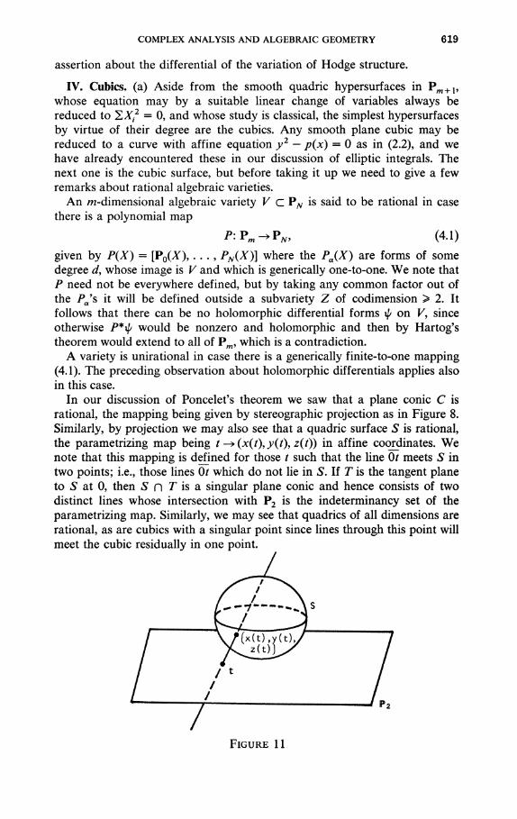
In our discussion of Poncelet's theorem we saw that a plane conic C is rational, the mapping being given by stereographic projection as in Figure 8. Similarly, by projection we may also see that a quadric surface S is rational, the parametrizing map being t-* (x(t), y(t), z(t)) in affine coordinates. We note that this mapping is defined for those / such that the line 0/ meets S in two points; i.e., those lines 0/ which do not lie in S. If T is the tangent plane to S at 0, then S n T is a singular plane conic and hence consists of two distinct lines whose intersection with P2 is the indeterminancy set of the parametrizing map. Similarly, we may see that quadrics of all dimensions are rational, as are cubics with a singular point since lines through this point will meet the cubic residually in one point.

I \ / (x( t ) ,v( t ) / 7

FIGURE 11

620 P. A. GRIFFITHS

When we turn to smooth cubics the picture changes. For example, the differential <o = dx/y given in (2.4) is everywhere holomorphic on the cubic plane curve (2.2), which cannot then be rational by our previous remark. It is this fact which lies at the root of the difficulty in understanding the elliptic integral, since there can be no change of variables reducing the integral to an elementary one as was possible, e.g., for the cardioid (2.19).

On the other, we saw in lecture three that the holomorphic differentials on a smooth cubic hypersurface in P w + 1 are residues of forms P(X)il/F(X) where deg P = 3 — (m + 2) (cf. (3.12)), and there are none of these if m > 2. In fact the cubic surface is rational.

To see why this should be so we first need to discuss the remarkable fact that there are on a smooth cubic hypersurface V c P w + 1 a family of oo2w~4

lines. Given points A = [A& . . . , Am+l] and B = [B& . . . , Bm+l] in Pm + 1 = P^"**2), the line joining them is parametrically described by t^A + txP. The set of all lines in P m + 1 is the Grassmann manifold G(l, m + 1), which has dimension 2m as may be seen by parametrizing a Zariski open set of lines by their points of intersection with two hyperplanes in Pm+1 . The vector A /\ B E P(A2Cm+2) represents the Plücker coordinates of the line and gives the usual embedding of the Grassmannian in a projective space Pr2+2)_1. Any geometric property of lines may be expressed in terms of these Plücker coordinates.

If F(X) = 0 is the equation of the cubic hypersurface V, then the above line lies in V exactly when F{ÎQA + txB) = 0. Expanding out we obtain

F(toA + * ! * ) « t30G0(A, B ) + tltxGx{A, B ) + t0t

2xG2(A9 B ) + t\G3(A, B ).

According to our remarks on Plücker coordinates the vector (G0(A, B)> GX(A, B), G2(A, B), G3(A, B)) = G(A A B) depends only on the Plücker coordinates of the line, and setting G(A /\B) = 0 defines a sub variety of codimension < 4 in G(l, m 4- 1). Thus the variety ^(V) of lines lying in V has dimension > 2m — 4. In fact, it was proved by the Italian geometer Fano that Sr( V) is smooth of dimension exactly 2m — 4, and is irreducible when m > 3.

When m = 2, dim 3F( V) = 0 and the Fano variety is the famous configuration of 27 lines on a cubic surface S. For our purposes all we need is the existence of one line L c S , using which we shall show that S is rational. For this we consider the pencil P2(s) of planes in P3 passing through L; this pencil has a rational parameter ^ e P , . For each s the intersection P2(s) • S is a plane cubic containing the line L, and therefore decomposes as

P2(s) S = L+ C(s)

where C(s) is a plane conic. By stereographic projection from one of the points of L • C(s) we may rationally parametrize C(s) by

/ -> (x{(s, t), x2(s, t\ x3(s, /))•

For a finite number of values s = st the conic C(s) splits into two lines and away from these critical values the functions xa(s, i) are locally single-valued functions of s as well as being rational functions of t. In fact, when s turns around a critical value s = st the Xj(s, i) analytically continue back to


themselves, a proof of which may be made by analogy with the following consideration:

FIGURE 12

In P2 we consider the family of conies C(s) having the affine equation 2 2

x — y = s.

FIGURE 13

When s = 0 the conic splits into the two lines x = ± y. Setting x = l/x' and y = y' / x' the equation of C(s) is

sx'2 + y'2 = 1.

From this we see that C(s) meets the line x' = 0 in the two points y' = ± 1. To explicitly give the stereographic projection of C(s) from x' = 0, y' = 1 we describe the pencil of lines through this point by the equation tx' + y' = 1. The residual point of intersection of this line with Cs has coordinates

It x =

s + t 2 '

/ = S + t 2 '

622 P. A. GRIFFITHS

which are then single-valued functions of both s and /. Returning to the cubic surface S, it follows that the x^s, t) are everywhere locally single-valued functions of s and are rational functions of t, and this observation may be developed into a proof that S is rational.

Coming to the cubic threefold V c P4 it was known 100 years ago and is not difficult to prove that V is unirational by a generically two-to-one map P3 -» V (cf. the references at the end of this talk). However, the preceding argument that a cubic surface is rational breaks down. It was Fano who believed that in fact V should not be rational, but all attempts to prove this by classical geometric arguments were incomplete and the nonrationality was only recently established. The combination of residues and Hodge theory played an important role in the original proof, and in a sense may be said to have provided the ingredient which the Italians were lacking. We shall conclude the lectures by very roughly describing how this goes.

(b) Some general considerations are necessary before we can go more deeply into the cubic threefold. If M is a smooth algebraic variety of odd dimension m = In + 1, we recall the Hodge decomposition (3.7) and set

H+(M) = H2n+l>°(M) 0 • • • @Hn+l-"(M)

= Fn + lHg£l(M). Integration over cycles defines a linear map

Z/2„+ 1(M,Z)-*#+(M)*,

and by virtue of H%£\M) = H+(M) 0 H + (M) the image of this map gives a lattice. The quotient

J(M) = H+(M)*/H2n+l(M, Z) (4.1)

is the intermediate Jacobian of M. For curves it is the usual Jacobian variety discussed in the previous two lectures.

As noted in the third lecture, J(M) varies holomorphically with M. However, when m > 1 the bilinear relations (3.9) do not give a polarization in the usual sense due to the alternation of signs in the last relation there. One case in which we do obtain a principal polarization is when

A 2*+i ,0 ( M ) = . . . = hn+2*-\(M) = 0 j h2n~\M) = 0, (4.2)

and under these circumstances we may expect the geometry of the 0-divisor to enter into the study of M. We note that when m = 3 the conditions (4.2) become

Z*3'°(M) = 0, A,(M) = 0. (4.3) To see how the geometry of 0 might enter we need an analogue of the

abelian sums on curves. If Z is an algebraic H-cycle on M which is homologous to zero, then following the same procedure as in the curve case we write Z = 3T for a chain T of real dimension In + 1 and consider the vector

K(Z) = (j \o, , . . . ,J\og)e/(M) (4.4)

where <o,, . . . , <og is a basis for H +(M). The map (4.4) which we may call the Abel-Jacobi map, has formal properties similar to the curve case. For exam-


pie, if { Wt}tGT is an algebraic family of «-dimensional algebraic subvarieties Wt c M, then choosing a base point 0 E T and setting Z, = Wt — W0 we obtain a holomorphic mapping

u: T->J(M).

The induced map on differentials is

u*:H+(M)-*#10(r),

and it follows that u is constant in case hx(T) = 0. In more suggestive notation the generalized "abelian sum"

(c- o) is constant mod periods in case the parameter variety T has first Betti number zero. For curves this is a fancy way of stating Abel's theorem.

We now return to our smooth cubic threefold F c P 4 with S = ^(V) denoting the Fano surface of lines on V. In this case by (3.14) and the Lefschetz hyperplane theorem the conditions (4.3) are satisfied, and we will study the Abel-Jacobi mapping

u:S-*J(V). (4.5)

The general version of Abel's theorem mentioned above gives the following two relations:

3

2 u(Lt) = const, Lv L2, L3 coplanar, i = i

6 2 u{La) = const, Ll9..., L6 pass through a point. (4.6)

a = l

Indeed, the planes P2 C P4 are rationally parametrized by the Grassmannian G(2, 4), and the intersection P2 • V = E is a plane cubic. Generically E is smooth, but it may degenerate into a line plus a conic or to three coplanar lines. In any case the abelian sum (/f co . . . , /f0<og) is constant mod periods, and this gives the first relation in (4.6). For the second one we note that at each point p of V the intersection Tp n V of the tangent plane with V is a cubic surface Sp with a singular point at p. It is easy to see that there are generically 6 lines La(p) through p lying in V, and since h\V) = 0 the corresponding abelian sum is constant mod periods.

The deeper properties of (4.5) require the interplay between residues and Hodge theory. Referring again to (3.14) we have:

The space H+(V) = H2,l(V) is canonically given by residues of rational forms

9"-7ü7 (47)

where H(X) E C5* is a linear function. In particular,

d i m / ( F ) = 5.

If we denote by Ls c V the line corresponding to s G S and by re(Ls) c

624 P. A. GRIFFITHS

P4 — V the e-tube over L5, then the Abel-Jacobi mapping (4.5) is described by integrals

limJ—^f^VA (4.8) Since <pH has a pole of order two along V the convergence of (4.8) is not obvious, but depends on the relation between order of pole and the Hodge type of cycles. However, once this has been established, it is quite plausible that the same reasoning should give the additional fact:

In case Ls is contained in the hyperplane H{X) = 0,

M Mm —J=/•*•%„)-a (4.9)

In other words, denoting by L,1- = C3 the subspace of C5* consisting of linear functions which vanish on the line Ls, what is suggested by these analytic considerations is a map

C5/LSX^TS(S)*. (4.10)

If this is true, then we have found a link between the infinitesimal properties of the Abel-Jacobi mapping (4.5) and the geometry of the surface of lines on the cubic threefold.

In fact, it turns out that (4.10) is defined as indicated and is an isomorphism. This implies that the composition of (4.5) with the Gauss mapping

y(M):S_>G(2,4),

which we recall assigns to each point u(s) E u(S) its tangent plane translated to the origin in C5 and viewed as a line in P4, is just the tautological inclusion of the Fano surface in the space of all lines in P4. This puts us in a formally analogous situation to the relationship as discussed in the third lecture between curves and their Jacobians, where the basic fact relating the Abelian sums and the projective geometry of the curve is the observation that the composition of u: C —» J(C) with the Gauss map is the canonical mapping of the curve. In the present case one may use (4.10) to get started on the analysis of the 0-divisor on J( V) which eventually leads to the nonrationality of the cubic threefold.

In concluding this discussion of cubics we should like to remark first that just as the Jacobian variety of a plane cubic may be given a group structure by taking the free group on the points modulo the relation "3 points are colinear" provided by Abel's theorem (2.13), so we may realize the intermediate Jacobian J( V) as the free group on the lines modulo the generating relations (4.6). Secondly, the analysis of the cubic has also been carried out over fields of any characteristic ih 2, so that there is no need to approach this-as well as any of the other problems we have discussed-by analytic methods if one doesn't so choose. The point I have hopefully been able to make is the continuing relevance of analytic methods to problems in algebraic geometry, both on aesthetic grounds and as a means of providing a method of attack on questions where purely geometric reasoning has yet to succeed.


REFERENCES

This is not intended to be a complete bibliography, but rather to list a few references either pertaining to the specific content of the lectures or to serve as a general source for background material where additional bibliography may be found.

Lecture one. The material from (a) may be found in Chapter V of [9], which also contains references to the more algebraic approach to residues. In addition to those sources we should like to also mention [2] and [4]. The Macaulay theorems from (b) appear in the classic monograph [15]. The applications of the global residue theorem from (c) are given in Chapter V of [9], and in greatly generalized form in [12].

Lecture two. An extensive discussion of the classical Abel's theorem appears in [7] from which much of (a) and (b) is taken. The Poncelet theorem is of course classical; the treatment in (c) is from [10] and [11], where the latter contains a generalization to polyhedral figures in space.

Lecture three. The details of the relationship between a curve and its. Jacobian are explained from the present point of view in Chapter II of [9]. An excellent alternate source is [17]. The basic results from Hodge theory are proved in Chapter I of [9], and the two expository papers [6] and [13] discuss recent developments and give a further bibliography. The material in (c) appears in [8], but the point of view in this lecture has been influenced by joint work in progress with Jim Carlson on the global Torelli theorem for hypersurfaces. The relationship between residues and Hodge theory has been extended to certain singular hypersurfaces, including those arising by generic projection of a smooth variety in a higher dimensional space, by Dave Morrison [16].

Lecture four. Our basic reference here is [3]. In addition, the cubic surface is discussed in Chapter IV of [9] and the general Fano schemes of lines lying in smooth hypersurfaces in [1] and [14]. Intermediate Jacobians of general threefolds are treated in the lectures of Turin [19], and the specific properties of the Abel-Jacobi map for the cubic appear there and in [3], which in particular gives (4.10) as "the tangent bundle theorem". Algebraic treatments of the rationality problem appear in [5] and [18].

1. A. Altman and S. Kleiman, Foundations of the theory of Fano schemes, Compositio Math. 34 (1977), 3-47.

2. A. Beauville, Une notion de residues en géométrie analytique, Séminaire Pierre Lelong (Analyse) 1970, Lecture Notes in Math., vol. 205, Springer-Verlag, Berlin and New York, 1971.

3. C. H. Clemens and P. Griffiths, The intermediate Jacobian of the cubic threefold, Ann. of Math. (2) 95 (1972), 281-356.

4. N. Coleff and M. Herrera, Les courants residues associés a une f orme méromorphe, preprint, Instituto Argentino de Mathematica, Viamante 1630, Buenos Aires.

5. A. Collino, A cheap proof of the irrationality of most cubic threefolds, Boll. Un. Mat. Ital. (to appear).

6. M. Cornalba and P. Griffiths, Some transcendental aspects of algebraic geometry, Proc. Sympos. Pure Math., vol. 29, Amer. Math. Soc, Providence, R. I., 1975, pp. 3-110.

7. P. Griffiths, Variations on a theorem of Abel, Invent. Math. 35 (1976), 321-390. 8. , On the periods of certain rational integrals. I, II, Ann. of Math. (2) 90 (1969),

460-495; 498-541. 9. P. Griffiths and J. Harris, Principles of algebraic geometry, Wiley, New York, 1978.

10. , On Cay ley9 s explicit solution to Poncelet9 s porism, L'Enseignement Math. 24 (1978), 31-40.

11. , A Poncelet theorem in space, Comment. Math. Helv. 52 (1977), 145-160. 12. , Residues and zero-cycles on algebraic varieties, Ann. of Math. 108 (1978), 461-505. 13. P. Griffiths and W. Schmid, Recent developments in Hodge theory: a discussion of techniques

and results, International Colloquium on Discrete Subgroups of Lie Groups and Moduli, Bombay (1973), Tata Institute, Bombay; Oxford Univ. Press, Bombay, 1975.

14. J. Harris, Galois groups of enumerative problems (to appear).

626 P. A. GRIFFITHS

15. F. S. Macaulay, The algebraic theory of modular systems, Cambridge Univ. Press, New York, 1916.

16. D. Morrison, Residues and the Hodge filtration for singular hypersurfaces (to appear). 17. D. Mumford, Curves and their Jacobians, Univ. of Michigan Press, Ann Arbor, Mich.,

1975. 18. J. Murre, Reduction of the proof of the non-rationality of a non-singular cubic threefold to a

result of Mumford, Compositio Math. 27 (1973), 63-82. 19. A. Turin, Five lectures on three dimensional varieties, Russian Math. Surveys 27 (1972),

3-50.

DEPARTMENT OF MATHEMATICS, HARVARD UNIVERSITY, CAMBRIDGE, MASSACHUSETTS 02138

volume 1, number 4, july 1979 - semantic scholar...bulletin (new series) of the american...

Documents