USER’S GUIDE FOR THE INDUSTRIALSOURCE COMPLEX (ISC3) DISPERSION

MODELS FOR USE IN THE MULTIMEDIA,MULTIPATHWAY AND MULTIRECEPTORRISK ASSESSMENT (3MRA) FOR HWIR99

VOLUME II: DESCRIPTION OF MODELALGORITHMS

DRAFT

Work Assignment Manager Donna B. Schwede and Technical Direction: U.S. Environmental Protection Agency

Office of Research and DevelopmentResearch Triangle Park, NC 27711

Prepared by: Pacific Environmental Services5001 South Miami Boulevard, Suite 300P.O. Box 12077Research Triangle Park, NC 27709-2077Under Contract No. 68-D7-0002 WA 1-001

U.S. Environmental Protection AgencyOffice of Solid Waste

Washington, DC 20460

June 30, 1999

ii

DISCLAIMER

The information in this document has been reviewed in its

entirety by the U.S. Environmental Protection Agency (EPA), and

approved for publication as an EPA document. Mention of trade

names, products, or services does not convey, and should not be

interpreted as conveying official EPA endorsement, or

recommendation.

iii

PREFACE

This User's Guide provides documentation for the

Industrial Source Complex (ISC3) models, referred to hereafter

as the Short Term (ISCST3) and Long Term (ISCLT3) models. This

volume describes the dispersion algorithms utilized in the

ISCST3 and ISCLT3 models, including the new area source and dry

deposition algorithms, both of which are a part of Supplement C

to the Guideline on Air Quality Models (Revised).

This volume also includes a technical description for the

following algorithms that are not included in Supplement C:

pit retention (ISCST3 and ISCLT3), wet deposition (ISCST3

only), and COMPLEX1 (ISCST3 only). The pit retention and wet

deposition algorithms have not undergone extensive evaluation

at this time, and their use is optional. COMPLEX1 is

incorporated to provide a means for conducting screening

estimates in complex terrain. EPA guidance on complex terrain

screening procedures is provided in Section 5.2.1 of the

Guideline on Air Quality Models (Revised).

Volume I of the ISC3 User's Guide provides user

instructions for the ISC3 models.

iv

ACKNOWLEDGEMENTS

The User's Guide for the ISC3 Models has been prepared by

Pacific Environmental Services, Inc., Research Triangle Park,

North Carolina. This effort has been funded by the

Environmental Protection Agency (EPA) under Contract No. 68-

D30032, with Desmond T. Bailey as Work Assignment Manager

(WAM). The technical description for the dry deposition

algorithm was developed from material prepared by Sigma

Research Corporation and funded by EPA under Contract No. 68-

D90067, with Jawad S. Touma as WAM.

v

CONTENTS

PREFACE . . . . . . . . . . . . . . . . . . . . . . . . . . iii

ACKNOWLEDGEMENTS . . . . . . . . . . . . . . . . . . . . . iv

FIGURES . . . . . . . . . . . . . . . . . . . . . . . . . . vii

TABLES . . . . . . . . . . . . . . . . . . . . . . . . . viii

SYMBOLS . . . . . . . . . . . . . . . . . . . . . . . . . . ix

1.0 THE ISC SHORT-TERM DISPERSION MODEL EQUATIONS . . . . . 1-11.1 POINT SOURCE EMISSIONS . . . . . . . . . . . . . . 1-2

1.1.1 The Gaussian Equation . . . . . . . . . . . 1-21.1.2 Downwind and Crosswind Distances . . . . . 1-31.1.3 Wind Speed Profile . . . . . . . . . . . . 1-41.1.4 Plume Rise Formulas . . . . . . . . . . . . 1-51.1.5 The Dispersion Parameters . . . . . . . . 1-151.1.6 The Vertical Term . . . . . . . . . . . . 1-311.1.7 The Decay Term . . . . . . . . . . . . . 1-39

1.2 NON-POINT SOURCE EMISSIONS . . . . . . . . . . . 1-401.2.1 General . . . . . . . . . . . . . . . . . 1-401.2.2 The Short-Term Volume Source Model . . . 1-411.2.3 The Short-Term Area Source Model . . . . 1-441.2.4 The Short-Term Open Pit Source Model . . 1-48

1.3 THE ISC SHORT-TERM DRY DEPOSITION MODEL . . . . 1-531.3.1 General . . . . . . . . . . . . . . . . . 1-531.3.2 Deposition and Gravitational Settling

Velocities . . . . . . . . . . . . . . . . 1-541.3.3 Point and Volume Source Emissions . . . . 1-591.3.4 Area and Open Pit Source Emissions . . . 1-60

1.4 THE ISC SHORT-TERM WET DEPOSITION MODEL . . . . 1-611.5 ISC COMPLEX TERRAIN SCREENING ALGORITHMS . . . . 1-63

1.5.1 The Gaussian Sector Average Equation . . 1-631.5.2 Downwind, Crosswind and Radial Distances 1-651.5.3 Wind Speed Profile . . . . . . . . . . . 1-651.5.4 Plume Rise Formulas . . . . . . . . . . . 1-651.5.5 The Dispersion Parameters . . . . . . . . 1-661.5.6 The Vertical Term . . . . . . . . . . . . 1-671.5.7 The Decay Term . . . . . . . . . . . . . 1-691.5.8 The Plume Attenuation Correction Factor . 1-691.5.9 Wet Deposition in Complex Terrain . . . 1-72

1.6 ISC TREATMENT OF INTERMEDIATE TERRAIN . . . . . 1-72

2.0 THE ISC LONG-TERM DISPERSION MODEL EQUATIONS . . . . . 2-1

vi

2.1 POINT SOURCE EMISSIONS . . . . . . . . . . . . . . 2-12.1.1 The Gaussian Sector Average Equation . . . 2-12.1.2 Downwind and Crosswind Distances . . . . . 2-42.1.3 Wind Speed Profile . . . . . . . . . . . . 2-42.1.4 Plume Rise Formulas . . . . . . . . . . . . 2-42.1.5 The Dispersion Parameters . . . . . . . . . 2-42.1.6 The Vertical Term . . . . . . . . . . . . . 2-62.1.7 The Decay Term . . . . . . . . . . . . . . 2-72.1.8 The Smoothing Function . . . . . . . . . . 2-7

2.2 NON-POINT SOURCE EMISSIONS . . . . . . . . . . . . 2-82.2.1 General . . . . . . . . . . . . . . . . . . 2-82.2.2 The Long-Term Volume Source Model . . . . . 2-82.2.3 The Long-Term Area Source Model . . . . . . 2-92.2.4 The Long-Term Open Pit Source Model . . . 2-12

2.3 THE ISC LONG-TERM DRY DEPOSITION MODEL . . . . . 2-122.3.1 General . . . . . . . . . . . . . . . . . 2-122.3.2 Point and Volume Source Emissions . . . . 2-132.3.3 Area and Open Pit Source Emissions . . . 2-14

3.0 REFERENCES . . . . . . . . . . . . . . . . . . . . . . 3-1

INDEX . . . . . . . . . . . . . . . . . . . . . . . . INDEX-1

vii

FIGURES

Figure Page

1-1 LINEAR DECAY FACTOR, A AS A FUNCTION OF EFFECTIVESTACK HEIGHT, He. A SQUAT BUILDING IS ASSUMED FORSIMPLICITY. . . . . . . . . . . . . . . . . . . . 1-71

1-2 ILLUSTRATION OF TWO TIERED BUILDING WITH DIFFERENTTIERS DOMINATING DIFFERENT WIND DIRECTIONS . . . . 1-72

1-3 THE METHOD OF MULTIPLE PLUME IMAGES USED TO SIMULATEPLUME REFLECTION IN THE ISC MODEL . . . . . . . . 1-73

1-4 SCHEMATIC ILLUSTRATION OF MIXING HEIGHT INTERPOLATIONPROCEDURES . . . . . . . . . . . . . . . . . . . . 1-74

1-5 ILLUSTRATION OF PLUME BEHAVIOR IN COMPLEX TERRAINASSUMED BY THE ISC MODEL . . . . . . . . . . . . . 1-75

1-6 ILLUSTRATION OF THE DEPLETION FACTOR FQ AND THECORRESPONDING PROFILE CORRECTION FACTOR P(x,z). . 1-76

1-7 VERTICAL PROFILE OF CONCENTRATION BEFORE AND AFTERAPPLYING FQ AND P(x,z) SHOWN IN FIGURE 1-6 . . . . 1-77

1-8 EXACT AND APPROXIMATE REPRESENTATION OF LINE SOURCE BYMULTIPLE VOLUME SOURCES . . . . . . . . . . . . . . 1-78

1-9 REPRESENTATION OF AN IRREGULARLY SHAPED AREA SOURCEBY 4 RECTANGULAR AREA SOURCES . . . . . . . . . . . 1-79

1-10 EFFECTIVE AREA AND ALONGWIND LENGTH FOR AN OPEN PITSOURCE . . . . . . . . . . . . . . . . . . . . . . . 1-80

1-11 WET SCAVENGING RATE COEFFICIENT AS A FUNCTION OF PARTICLESIZE (JINDAL & HEINOLD, 1991) . . . . . . . . . . . 1-81

viii

TABLES

Table Page

PARAMETERS USED TO CALCULATE PASQUILL-GIFFORD Fy . . . . 1-16PARAMETERS USED TO CALCULATE PASQUILL-GIFFORD Fz . . . . 1-17BRIGGS FORMULAS USED TO CALCULATE McELROY-POOLER Fy . . . 1-19BRIGGS FORMULAS USED TO CALCULATE McELROY-POOLER Fz . . . 1-19COEFFICIENTS USED TO CALCULATE LATERAL VIRTUAL DISTANCES

FOR PASQUILL-GIFFORD DISPERSION RATES . . . 1-21SUMMARY OF SUGGESTED PROCEDURES FOR ESTIMATING

INITIAL LATERAL DIMENSIONS Fyo ANDINITIAL VERTICAL DIMENSIONS Fzo FOR VOLUME AND LINE SOURCES1-43

ix

SYMBOLS

Symbol Definition

A Linear decay term for vertical dispersion inSchulman-Scire downwash (dimensionless)

Ae Effective area for open pit emissions (dimensionless)

D Exponential decay term for Gaussian plume equation(dimensionless)

DB Brownian diffusivity (cm/s)

Dr Relative pit depth (dimensionless)

de Effective pit depth (m)

dp Particle diameter for particulate emissions (:m)

ds Stack inside diameter (m)

Fb Buoyancy flux parameter (m4/s3)

Fd Dry deposition flux (g/m2)

Fm Momentum flux parameter (m4/s2)

FQ Plume depletion factor for dry deposition(dimensionless)

FT Terrain adjustment factor (dimensionless)

Fw Wet deposition flux (g/m2)

f Frequency of occurrence of a wind speed and stabilitycategory combination (dimensionless)

g Acceleration due to gravity (9.80616 m/s2)

hb Building height (m)

he Plume (or effective stack) height (m)

hs Physical stack height (m)

x

hter Height of terrain above stack base (m)

hs' Release height modified for stack-tip downwash (m)

hw Crosswind projected width of building adjacent to astack (m)

k von Karman constant (= 0.4)

L Monin-Obukhov length (m)

Ly Initial plume length for Schulman-Scire downwashsources with enhanced lateral plume spread (m)

Lb Lesser of the building height and crosswind projectedbuilding width (m)

R Alongwind length of open pit source (m)

P(x,y) Profile adjustment factor (dimensionless)

p Wind speed power law profile exponent (dimensionless)

QA Area Source pollutant emission rate (g/s)

Qe Effective emission rate for effective area source foran open pit source (g/s)

Qi Adjusted emission rate for particle size category foropen pit emissions (g/s)

Qs Pollutant emission rate (g/s)

QJ Total amount of pollutant emitted during time period J(g)

R Precipitation rate (mm/hr)

Ro Initial plume radius for Schulman-Scire downwashsources (m)

R(z,zd) Atmospheric resistance to vertical transport (s/cm)

r Radial distance range in a polar receptor network (m)

xi

ra Atmospheric resistance (s/cm)

rd Deposition layer resistance (s/cm)

s Stability parameter =

S Smoothing term for smoothing across adjacent sectors inthe Long Term model (dimensionless)

SCF Splip correction factor (dimensionless)

Sc Schmidt number = (dimensionless)

St Stokes number = (dimensionless)

Ta Ambient temperature (K)

Ts Stack gas exit temperature (K)

uref Wind speed measured at reference anemometer height(m/s)

us Wind speed adjusted to release height (m/s)

u* Surface friction velocity (m/s)

V Vertical term of the Gaussian plume equation(dimensionless)

Vd Vertical term with dry deposition of the Gaussian plumeequation (dimensionless)

vd Particle deposition velocity (cm/s)

vg Gravitational settling velocity for particles (cm/s)

vs Stack gas exit velocity (m/s)

X X-coordinate in a Cartesian grid receptor network (m)

xo Length of side of square area source (m)

Y Y-coordinate in a Cartesian grid receptor network (m)

xii

2 Direction in a polar receptor network (degrees)

x Downwind distance from source to receptor (m)

xy Lateral virtual point source distance (m)

xz Vertical virtual point source distance (m)

xf Downwind distance to final plume rise (m)

x* Downwind distance at which turbulence dominatesentrainment (m)

y Crosswind distance from source to receptor (m)

z Receptor/terrain height above mean sea level (m)

zd Dry deposition reference height (m)

zr Receptor height above ground level (i.e. flagpole) (m)

zref Reference height for wind speed power law (m)

zs Stack base elevation above mean sea level (m)

zi Mixing height (m)

z0 Surface roughness height (m)

$ Entrainment coefficient used in buoyant rise forSchulman-Scire downwash sources = 0.6

$j Jet entrainment coefficient used in gradual momentum

plume rise calculations

)h Plume rise (m)

M2/Mz Potential temperature gradient with height (K/m)

gi Escape fraction of particle size category for open pitemissions (dimensionless)

7 Precipitation scavenging ratio (s-1)

xiii

8 Precipitation rate coefficient (s-mm/hr)-1

B pi = 3.14159

R Decay coefficient = 0.693/T1/2 (s-1)

RH Stability adjustment factor (dimensionless)

N Fraction of mass in a particular settling velocitycategory for particulates (dimensionless)

D Particle density (g/cm3)

DAIR Density of air (g/cm3)

Fy Horizontal (lateral) dispersion parameter (m)

Fyo Initial horizontal dispersion parameter for virtualpoint source (m)

Fye Effective lateral dispersion parameter includingeffects of buoyancy-induced dispersion (m)

Fz Vertical dispersion parameter (m)

Fzo Initial vertical dispersion parameter for virtual pointsource (m)

Fze Effective vertical dispersion parameter includingeffects of buoyancy-induced dispersion (m)

L Viscosity of air ï 0.15 cm2/s

: Absolute viscosity of air ï 1.81 x 10-4 g/cm/s

P Concentration (:g/m3)

Pd Concentration with dry deposition effects (:g/m3)

1-1

1.0 THE ISC SHORT-TERM DISPERSION MODEL EQUATIONS

The Industrial Source Complex (ISC) Short Term model

provides options to model emissions from a wide range of

sources that might be present at a typical industrial source

complex. The basis of the model is the straight-line,

steady-state Gaussian plume equation, which is used with some

modifications to model simple point source emissions from

stacks, emissions from stacks that experience the effects of

aerodynamic downwash due to nearby buildings, isolated vents,

multiple vents, storage piles, conveyor belts, and the like.

Emission sources are categorized into four basic types of

sources, i.e., point sources, volume sources, area sources, and

open pit sources. The volume source option and the area source

option may also be used to simulate line sources. The

algorithms used to model each of these source types are

described in detail in the following sections. The point

source algorithms are described in Section 1.1. The volume,

area and open pit source model algorithms are described in

Section 1.2. Section 1.3 gives the optional algorithms for

calculating dry deposition for point, volume, area and open pit

sources, and Section 1.4 describes the optional algorithms for

calculating wet deposition. Sections 1.1 through 1.4 describe

calculations for simple terrain (defined as terrain elevations

below the release height). The modifications to these

calculations to account for complex terrain are described in

Section 1.5, and the treatment of intermediate terrain is

discussed in Section 1.6.

The ISC Short Term model accepts hourly meteorological

data records to define the conditions for plume rise,

transport, diffusion, and deposition. The model estimates the

concentration or deposition value for each source and receptor

1-2

combination for each hour of input meteorology, and calculates

user-selected short-term averages. For deposition values,

either the dry deposition flux, the wet deposition flux, or the

total deposition flux may be estimated. The total deposition

flux is simply the sum of the dry and wet deposition fluxes at

a particular receptor location. The user also has the option

of selecting averages for the entire period of input

meteorology.

1.1 POINT SOURCE EMISSIONS

The ISC Short Term model uses a steady-state Gaussian

plume equation to model emissions from point sources, such as

stacks and isolated vents. This section describes the Gaussian

point source model, including the basic Gaussian equation, the

plume rise formulas, and the formulas used for determining

dispersion parameters.

1.1.1 The Gaussian Equation

The ISC short term model for stacks uses the steady-state

Gaussian plume equation for a continuous elevated source. For

each source and each hour, the origin of the source's

coordinate system is placed at the ground surface at the base

of the stack. The x axis is positive in the downwind

direction, the y axis is crosswind (normal) to the x axis and

the z axis extends vertically. The fixed receptor locations

are converted to each source's coordinate system for each

hourly concentration calculation. The calculation of the

downwind and crosswind distances is described in Section 1.1.2.

The hourly concentrations calculated for each source at each

receptor are summed to obtain the total concentration produced

at each receptor by the combined source emissions.

1-3

(1-1)

For a steady-state Gaussian plume, the hourly

concentration at downwind distance x (meters) and crosswind

distance y (meters) is given by:

where:

Q = pollutant emission rate (mass per unit time)

K = a scaling coefficient to convert calculatedconcentrations to desired units (default value of1 x 106 for Q in g/s and concentration in :g/m3)

V = vertical term (See Section 1.1.6)

D = decay term (See Section 1.1.7)

Fy,Fz = standard deviation of lateral and verticalconcentration distribution (m) (See Section1.1.5)

us = mean wind speed (m/s) at release height (SeeSection 1.1.3)

Equation (1-1) includes a Vertical Term (V), a Decay Term

(D), and dispersion parameters (Fy and Fz) as discussed below.

It should be noted that the Vertical Term includes the effects

of source elevation, receptor elevation, plume rise, limited

mixing in the vertical, and the gravitational settling and dry

deposition of particulates (with diameters greater than about

0.1 microns).

1.1.2 Downwind and Crosswind Distances

The ISC model uses either a polar or a Cartesian receptor

network as specified by the user. The model allows for the use

of both types of receptors and for multiple networks in a

1-4

(1-2)

(1-3)

(1-4)

single run. All receptor points are converted to Cartesian

(X,Y) coordinates prior to performing the dispersion

calculations. In the polar coordinate system, the radial

coordinate of the point (r, 2) is measured from the

user-specified origin and the angular coordinate 2 is measured

clockwise from the north. In the Cartesian coordinate system,

the X axis is positive to the east of the user-specified origin

and the Y axis is positive to the north. For either type of

receptor network, the user must define the location of each

source with respect to the origin of the grid using Cartesian

coordinates. In the polar coordinate system, assuming the

origin is at X = Xo, Y = Yo, the X and Y coordinates of a

receptor at the point (r, 2) are given by:

If the X and Y coordinates of the source are X(S) and Y(S), the

downwind distance x to the receptor, along the direction of

plume travel, is given by:

where WD is the direction from which the wind is blowing. The

downwind distance is used in calculating the distance-dependent

plume rise (see Section 1.1.4) and the dispersion parameters

(see Section 1.1.5). If any receptor is located within 1 meter

of a point source or within 1 meter of the effective radius of

a volume source, a warning message is printed and no

concentrations are calculated for the source-receptor

1-5

(1-5)

(1-6)

combination. The crosswind distance y to the receptor from the

plume centerline is given by:

The crosswind distance is used in Equation (1-1).

1.1.3 Wind Speed Profile

The wind power law is used to adjust the observed wind

speed, uref, from a reference measurement height, zref, to the

stack or release height, hs. The stack height wind speed, us,

is used in the Gaussian plume equation (Equation 1-1), and in

the plume rise formulas described in Section 1.1.4. The power

law equation is of the form:

where p is the wind profile exponent. Values of p may be

provided by the user as a function of stability category and

wind speed class. Default values are as follows:

Stability Category Rural Exponent Urban Exponent

A 0.07 0.15

B 0.07 0.15

C 0.10 0.20

D 0.15 0.25

E 0.35 0.30

F 0.55 0.30

The stack height wind speed, us, is not allowed to be less

than 1.0 m/s.

1-6

(1-7)

1.1.4 Plume Rise Formulas

The plume height is used in the calculation of the

Vertical Term described in Section 1.1.6. The Briggs plume

rise equations are discussed below. The description follows

Appendix B of the Addendum to the MPTER User's Guide (Chico and

Catalano, 1986) for plumes unaffected by building wakes. The

distance dependent momentum plume rise equations, as described

in (Bowers, et al., 1979), are used to determine if the plume

is affected by the wake region for building downwash

calculations. These plume rise calculations for wake

determination are made assuming no stack-tip downwash for both

the Huber-Snyder and the Schulman-Scire methods. When the

model executes the building downwash methods of Schulman and

Scire, the reduced plume rise suggestions of Schulman and Scire

(1980) are used, as described in Section 1.1.4.11.

1.1.4.1 Stack-tip Downwash.

In order to consider stack-tip downwash, modification of

the physical stack height is performed following Briggs (1974,

p. 4). The modified physical stack height hs' is found from:

where hs is physical stack height (m), vs is stack gas exit

velocity (m/s), and ds is inside stack top diameter (m). This

hs' is used throughout the remainder of the plume height

1-7

(1-8)

(1-9)

(1-10)

computation. If stack tip downwash is not considered, hs' = hsin the following equations.

1.1.4.2 Buoyancy and Momentum Fluxes.

For most plume rise situations, the value of the Briggs

buoyancy flux parameter, Fb (m4/s3), is needed. The following

equation is equivalent to Equation (12), (Briggs, 1975, p. 63):

where )T = Ts - Ta, Ts is stack gas temperature (K), and Ta is

ambient air temperature (K).

For determining plume rise due to the momentum of the

plume, the momentum flux parameter, Fm (m4/s2), is calculated

based on the following formula:

1.1.4.3 Unstable or Neutral - Crossover Between Momentumand Buoyancy.

For cases with stack gas temperature greater than or equal

to ambient temperature, it must be determined whether the plume

rise is dominated by momentum or buoyancy. The crossover

temperature difference, ()T)c, is determined by setting Briggs'

(1969, p. 59) Equation 5.2 equal to the combination of Briggs'

(1971, p. 1031) Equations 6 and 7, and solving for )T, as

follows:

for Fb < 55,

1-8

(1-11)

(1-12)

(1-13)

(1-14)

and for Fb $ 55,

If the difference between stack gas and ambient temperature,

)T, exceeds or equals ()T)c, plume rise is assumed to be

buoyancy dominated, otherwise plume rise is assumed to be

momentum dominated.

1.1.4.4 Unstable or Neutral - Buoyancy Rise.

For situations where )T exceeds ()T)c as determined above,

buoyancy is assumed to dominate. The distance to final rise,

xf, is determined from the equivalent of Equation (7), (Briggs,

1971, p. 1031), and the distance to final rise is assumed to be

3.5x*, where x* is the distance at which atmospheric turbulence

begins to dominate entrainment. The value of xf is calculated

as follows:

for Fb < 55:

and for Fb $ 55:

The final effective plume height, he (m), is determined

from the equivalent of the combination of Equations (6) and (7)

(Briggs, 1971, p. 1031):

for Fb < 55:

1-9

(1-15)

(1-16)

(1-17)

and for Fb $ 55:

1.1.4.5 Unstable or Neutral - Momentum Rise.

For situations where the stack gas temperature is less

than or equal to the ambient air temperature, the assumption is

made that the plume rise is dominated by momentum. If )T is

less than ()T)c from Equation (1-10) or (1-11), the assumption

is also made that the plume rise is dominated by momentum. The

plume height is calculated from Equation (5.2) (Briggs, 1969,

p. 59):

Briggs (1969, p. 59) suggests that this equation is most

applicable when vs/us is greater than 4.

1.1.4.6 Stability Parameter.

For stable situations, the stability parameter, s, is

calculated from the Equation (Briggs, 1971, p. 1031):

As a default approximation, for stability class E (or 5) M2/Mz

is taken as 0.020 K/m, and for class F (or 6), M2/Mz is taken

as 0.035 K/m.

1-10

(1-18)

(1-19)

(1-20)

1.1.4.7 Stable - Crossover Between Momentum and Buoyancy.

For cases with stack gas temperature greater than or equal

to ambient temperature, it must be determined whether the plume

rise is dominated by momentum or buoyancy. The crossover

temperature difference, ()T)c , is determined by setting

Briggs' (1975, p. 96) Equation 59 equal to Briggs' (1969, p.

59) Equation 4.28, and solving for )T, as follows:

If the difference between stack gas and ambient temperature,

)T, exceeds or equals ()T)c, plume rise is assumed to be

buoyancy dominated, otherwise plume rise is assumed to be

momentum dominated.

1.1.4.8 Stable - Buoyancy Rise.

For situations where )T exceeds ()T)c as determined above,

buoyancy is assumed to dominate. The distance to final rise,

xf, is determined by the equivalent of a combination of

Equations (48) and (59) in Briggs, (1975), p. 96:

The plume height, he, is determined by the equivalent of

Equation (59) (Briggs, 1975, p. 96):

1-11

(1-21)

(1-22)

1.1.4.9 Stable - Momentum Rise.

Where the stack gas temperature is less than or equal to

the ambient air temperature, the assumption is made that the

plume rise is dominated by momentum. If )T is less than ()T)c

as determined by Equation (1-18), the assumption is also made

that the plume rise is dominated by momentum. The plume height

is calculated from Equation 4.28 of Briggs ((1969), p. 59):

The equation for unstable-neutral momentum rise (1-16) is also

evaluated. The lower result of these two equations is used as

the resulting plume height, since stable plume rise should not

exceed unstable-neutral plume rise.

1.1.4.10 All Conditions - Distance Less Than Distance toFinal Rise.

Where gradual rise is to be estimated for unstable,

neutral, or stable conditions, if the distance downwind from

source to receptor, x, is less than the distance to final rise,

the equivalent of Equation 2 of Briggs ((1972), p. 1030) is

used to determine plume height:

This height will be used only for buoyancy dominated

conditions; should it exceed the final rise for the appropriate

condition, the final rise is substituted instead.

1-12

(1-23)

(1-24)

(1-25)

(1-26)

(1-27)

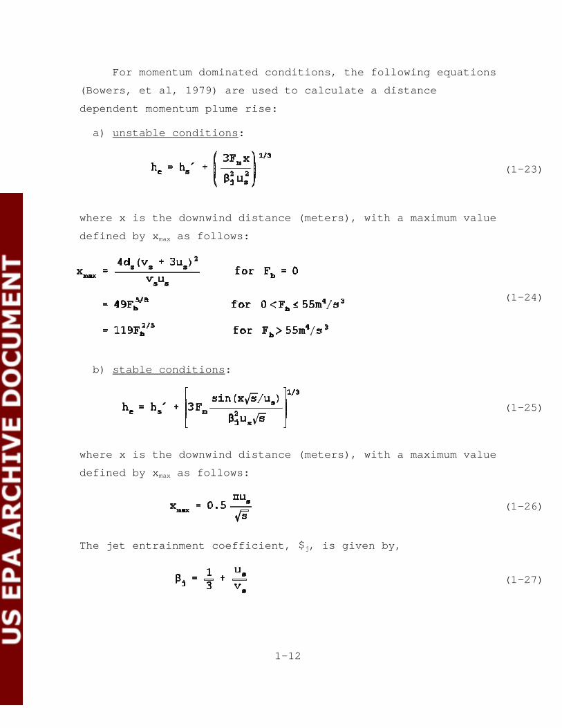
For momentum dominated conditions, the following equations

(Bowers, et al, 1979) are used to calculate a distance

dependent momentum plume rise:

a) unstable conditions:

where x is the downwind distance (meters), with a maximum value

defined by xmax as follows:

b) stable conditions:

where x is the downwind distance (meters), with a maximum value

defined by xmax as follows:

The jet entrainment coefficient, $j, is given by,

1-13

As with the buoyant gradual rise, if the distance-dependent

momentum rise exceeds the final rise for the appropriate

condition, then the final rise is substituted instead.

1.1.4.10.1 Calculating the plume height for wake effectsdetermination.

The building downwash algorithms in the ISC models always

require the calculation of a distance dependent momentum plume

rise. When building downwash is being simulated, the equations

described above are used to calculate a distance dependent

momentum plume rise at a distance of two building heights

downwind from the leeward edge of the building. However,

stack-tip downwash is not used when performing this calculation

(i.e. hs' = hs). This wake plume height is compared to the

wake height based on the good engineering practice (GEP)

formula to determine whether the building wake effects apply to

the plume for that hour.

The procedures used to account for the effects of building

downwash are discussed more fully in Section 1.1.5.3. The

plume rise calculations used with the Schulman-Scire algorithm

are discussed in Section 1.1.4.11.

1.1.4.11 Plume Rise When Schulman and Scire BuildingDownwash is Selected.

The Schulman-Scire downwash algorithms are used by the ISC

models when the stack height is less than the building height

plus one half of the lesser of the building height or width.

When these criteria are met, the ISC models estimate plume rise

during building downwash conditions following the suggestion of

Scire and Schulman (1980). The plume rise during building

1-14

(1-28)

(1-29a)

(1-30)

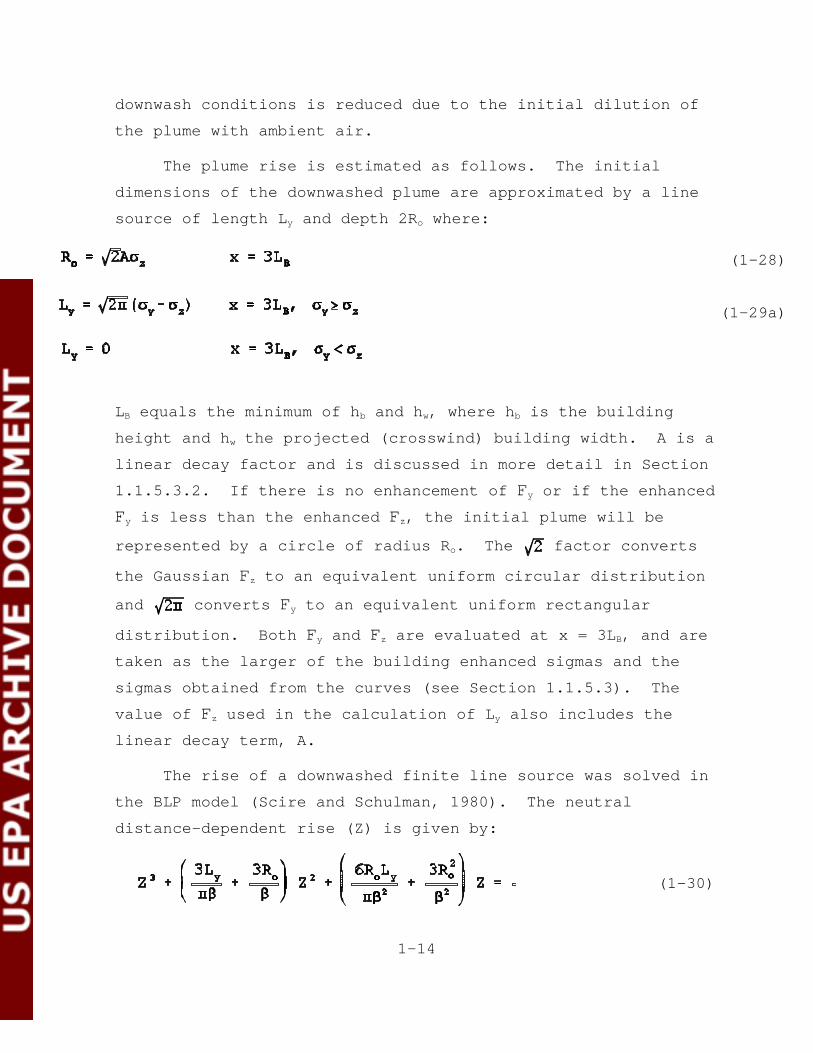
downwash conditions is reduced due to the initial dilution of

the plume with ambient air.

The plume rise is estimated as follows. The initial

dimensions of the downwashed plume are approximated by a line

source of length Ly and depth 2Ro where:

LB equals the minimum of hb and hw, where hb is the building

height and hw the projected (crosswind) building width. A is a

linear decay factor and is discussed in more detail in Section

1.1.5.3.2. If there is no enhancement of Fy or if the enhanced

Fy is less than the enhanced Fz, the initial plume will be

represented by a circle of radius Ro. The factor converts

the Gaussian Fz to an equivalent uniform circular distribution

and converts Fy to an equivalent uniform rectangular

distribution. Both Fy and Fz are evaluated at x = 3LB, and are

taken as the larger of the building enhanced sigmas and the

sigmas obtained from the curves (see Section 1.1.5.3). The

value of Fz used in the calculation of Ly also includes the

linear decay term, A.

The rise of a downwashed finite line source was solved in

the BLP model (Scire and Schulman, 1980). The neutral

distance-dependent rise (Z) is given by:

1-15

(1-31a)

(1-31b)

The stable distance-dependent rise is calculated by:

with a maximum stable buoyant rise given by:

where:

Fb = buoyancy flux term (Equation 1-8) (m4/s3)

Fm = momentum flux term (Equation 1-9) (m4/s2)

x = downwind distance (m)

us = wind speed at release height (m/s)

vs = stack exit velocity (m/s)

ds = stack diameter (m)

$ = entrainment coefficient (=0.6)

$j= jet entrainment coefficient

s = stability parameter

The larger of momentum and buoyant rise, determined separately

by alternately setting Fb or Fm = 0 and solving for Z, is

selected for plume height calculations for Schulman-Scire

downwash. In the ISC models, Z is determined by solving the

cubic equation using Newton's method.

1-16

(1-32)

(1-33)

(1-34)

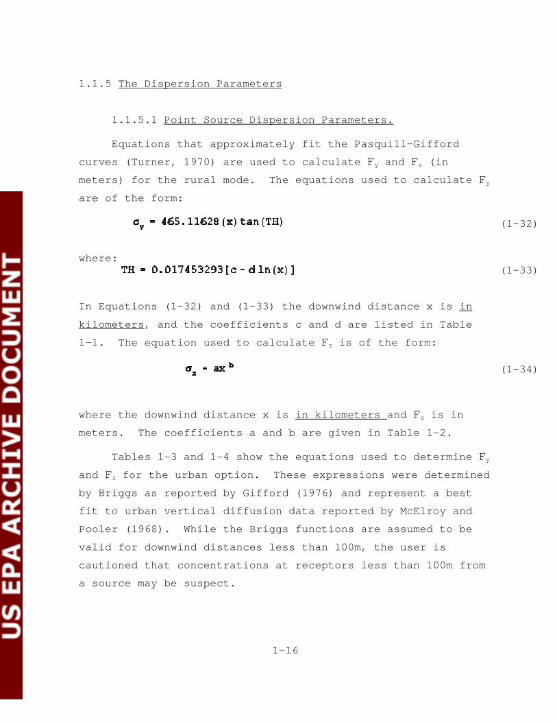
1.1.5 The Dispersion Parameters

1.1.5.1 Point Source Dispersion Parameters.

Equations that approximately fit the Pasquill-Gifford

curves (Turner, 1970) are used to calculate Fy and Fz (in

meters) for the rural mode. The equations used to calculate Fy

are of the form:

where:

In Equations (1-32) and (1-33) the downwind distance x is in

kilometers, and the coefficients c and d are listed in Table

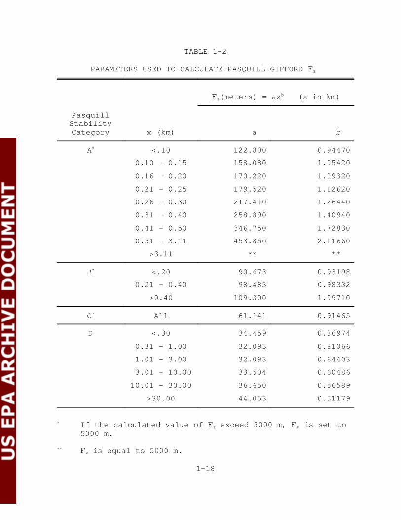
1-1. The equation used to calculate Fz is of the form:

where the downwind distance x is in kilometers and Fz is in

meters. The coefficients a and b are given in Table 1-2.

Tables 1-3 and 1-4 show the equations used to determine Fy

and Fz for the urban option. These expressions were determined

by Briggs as reported by Gifford (1976) and represent a best

fit to urban vertical diffusion data reported by McElroy and

Pooler (1968). While the Briggs functions are assumed to be

valid for downwind distances less than 100m, the user is

cautioned that concentrations at receptors less than 100m from

a source may be suspect.

1-17

TABLE 1-1

PARAMETERS USED TO CALCULATE PASQUILL-GIFFORD Fy

Fy = 465.11628 (x)tan(TH)

TH = 0.017453293 [c - d ln(x)]

PasquillStabilityCategory c d

A 24.1670 2.5334

B 18.3330 1.8096

C 12.5000 1.0857

D 8.3330 0.72382

E 6.2500 0.54287

F 4.1667 0.36191

where Fy is in meters and x is in kilometers

1-18

TABLE 1-2

PARAMETERS USED TO CALCULATE PASQUILL-GIFFORD Fz

Fz(meters) = axb (x in km)

PasquillStabilityCategory x (km) a b

A* <.10

0.10 - 0.15

0.16 - 0.20

0.21 - 0.25

0.26 - 0.30

0.31 - 0.40

0.41 - 0.50

0.51 - 3.11

>3.11

122.800

158.080

170.220

179.520

217.410

258.890

346.750

453.850

**

0.94470

1.05420

1.09320

1.12620

1.26440

1.40940

1.72830

2.11660

**

B* <.20

0.21 - 0.40

>0.40

90.673

98.483

109.300

0.93198

0.98332

1.09710

C* All 61.141 0.91465

D <.30

0.31 - 1.00

1.01 - 3.00

3.01 - 10.00

10.01 - 30.00

>30.00

34.459

32.093

32.093

33.504

36.650

44.053

0.86974

0.81066

0.64403

0.60486

0.56589

0.51179

* If the calculated value of Fz exceed 5000 m, Fz is set to5000 m.

** Fz is equal to 5000 m.

1-19

TABLE 1-2(CONTINUED)

PARAMETERS USED TO CALCULATE PASQUILL-GIFFORD Fz

Fz(meters) = axb (x in km)

PasquillStabilityCategory x (km) a b

E <.10

0.10 - 0.30

0.31 - 1.00

1.01 - 2.00

2.01 - 4.00

4.01 - 10.00

10.01 - 20.00

20.01 - 40.00

>40.00

24.260

23.331

21.628

21.628

22.534

24.703

26.970

35.420

47.618

0.83660

0.81956

0.75660

0.63077

0.57154

0.50527

0.46713

0.37615

0.29592

F <.20

0.21 - 0.70

0.71 - 1.00

1.01 - 2.00

2.01 - 3.00

3.01 - 7.00

7.01 - 15.00

15.01 - 30.00

30.01 - 60.00

>60.00

15.209

14.457

13.953

13.953

14.823

16.187

17.836

22.651

27.074

34.219

0.81558

0.78407

0.68465

0.63227

0.54503

0.46490

0.41507

0.32681

0.27436

0.21716

1-20

TABLE 1-3

BRIGGS FORMULAS USED TO CALCULATE McELROY-POOLER Fy

PasquillStabilityCategory Fy(meters)*

A 0.32 x (1.0 + 0.0004 x)-1/2

B 0.32 x (1.0 + 0.0004 x)-1/2

C 0.22 x (1.0 + 0.0004 x)-1/2

D 0.16 x (1.0 + 0.0004 x)-1/2

E 0.11 x (1.0 + 0.0004 x)-1/2

F 0.11 x (1.0 + 0.0004 x)-1/2

* Where x is in meters

TABLE 1-4

BRIGGS FORMULAS USED TO CALCULATE McELROY-POOLER Fz

PasquillStabilityCategory Fz(meters)*

A 0.24 x (1.0 + 0.001 x)1/2

B 0.24 x (1.0 + 0.001 x)1/2

C 0.20 x

D 0.14 x (1.0 + 0.0003 x)-1/2

E 0.08 x (1.0 + 0.0015 x)-1/2

F 0.08 x (1.0 + 0.0015 x)-1/2

* Where x is in meters.

1-21

(1-35)

(1-36)

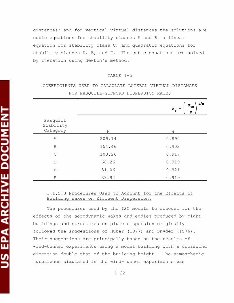
1.1.5.2 Lateral and Vertical Virtual Distances.

The equations in Tables 1-1 through 1-4 define the

dispersion parameters for an ideal point source. However,

volume sources have initial lateral and vertical dimensions.

Also, as discussed below, building wake effects can enhance the

initial growth of stack plumes. In these cases, lateral (xy)

and vertical (xz) virtual distances are added by the ISC models

to the actual downwind distance x for the Fy and Fz

calculations. The lateral virtual distance in kilometers for

the rural mode is given by:

where the stability-dependent coefficients p and q are given in

Table 1-5 and Fyo is the standard deviation in meters of the

lateral concentration distribution at the source. Similarly,

the vertical virtual distance in kilometers for the rural mode

is given by:

where the coefficients a and b are obtained form Table 1-2 and

Fzo is the standard deviation in meters of the vertical

concentration distribution at the source. It is important to

note that the ISC model programs check to ensure that the xz

used to calculate Fz at (x + xz) in the rural mode is the xz

calculated using the coefficients a and b that correspond to

the distance category specified by the quantity (x + xz).

To determine virtual distances for the urban mode, the

functions displayed in Tables 1-3 and 1-4 are solved for x.

The solutions are quadratic formulas for the lateral virtual

1-22

distances; and for vertical virtual distances the solutions are

cubic equations for stability classes A and B, a linear

equation for stability class C, and quadratic equations for

stability classes D, E, and F. The cubic equations are solved

by iteration using Newton's method.

TABLE 1-5

COEFFICIENTS USED TO CALCULATE LATERAL VIRTUAL DISTANCES

FOR PASQUILL-GIFFORD DISPERSION RATES

PasquillStabilityCategory p q

A 209.14 0.890

B 154.46 0.902

C 103.26 0.917

D 68.26 0.919

E 51.06 0.921

F 33.92 0.919

1.1.5.3 Procedures Used to Account for the Effects ofBuilding Wakes on Effluent Dispersion.

The procedures used by the ISC models to account for the

effects of the aerodynamic wakes and eddies produced by plant

buildings and structures on plume dispersion originally

followed the suggestions of Huber (1977) and Snyder (1976).

Their suggestions are principally based on the results of

wind-tunnel experiments using a model building with a crosswind

dimension double that of the building height. The atmospheric

turbulence simulated in the wind-tunnel experiments was

1-23

intermediate between the turbulence intensity associated with

the slightly unstable Pasquill C category and the turbulence

intensity associated with the neutral D category. Thus, the

data reported by Huber and Snyder reflect a specific stability,

building shape and building orientation with respect to the

mean wind direction. It follows that the ISC wake-effects

evaluation procedures may not be strictly applicable to all

situations. The ISC models also provide for the revised

treatment of building wake effects for certain sources, which

uses modified plume rise algorithms, following the suggestions

of Schulman and Hanna (1986). This treatment is largely based

on the work of Scire and Schulman (1980). When the stack

height is less than the building height plus half the lesser of

the building height or width, the methods of Schulman and Scire

are followed. Otherwise, the methods of Huber and Snyder are

followed. In the ISC models, direction-specific building

dimensions may be used with either the Huber-Snyder or

Schulman-Scire downwash algorithms.

The wake-effects evaluation procedures may be applied by

the user to any stack on or adjacent to a building. For

regulatory application, a building is considered sufficiently

close to a stack to cause wake effects when the distance

between the stack and the nearest part of the building is less

than or equal to five times the lesser of the height or the

projected width of the building. For downwash analyses with

direction-specific building dimensions, wake effects are

assumed to occur if the stack is within a rectangle composed of

two lines perpendicular to the wind direction, one at 5Lb

downwind of the building and the other at 2Lb upwind of the

building, and by two lines parallel to the wind direction, each

at 0.5Lb away from each side of the building, as shown below:

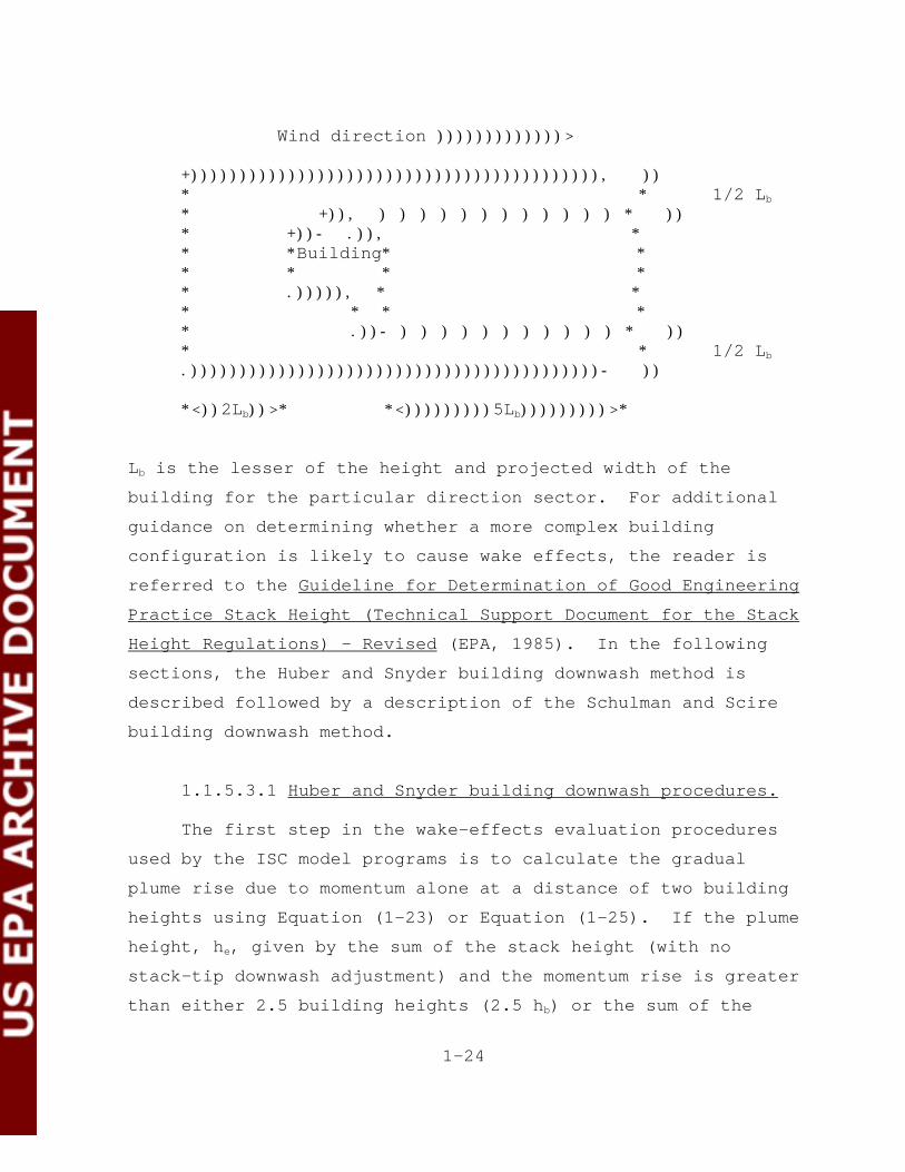
1-24

Wind direction )))))))))))))>

+)))))))))))))))))))))))))))))))))))))))))), ))* * 1/2 Lb* +)), ) ) ) ) ) ) ) ) ) ) ) ) * ))* +))- .)), ** *Building* ** * * ** .))))), * ** * * ** .))- ) ) ) ) ) ) ) ) ) ) ) * ))* * 1/2 Lb.))))))))))))))))))))))))))))))))))))))))))- ))

*<))2Lb))>* *<)))))))))5Lb)))))))))>*

Lb is the lesser of the height and projected width of the

building for the particular direction sector. For additional

guidance on determining whether a more complex building

configuration is likely to cause wake effects, the reader is

referred to the Guideline for Determination of Good Engineering

Practice Stack Height (Technical Support Document for the Stack

Height Regulations) - Revised (EPA, 1985). In the following

sections, the Huber and Snyder building downwash method is

described followed by a description of the Schulman and Scire

building downwash method.

1.1.5.3.1 Huber and Snyder building downwash procedures.

The first step in the wake-effects evaluation procedures

used by the ISC model programs is to calculate the gradual

plume rise due to momentum alone at a distance of two building

heights using Equation (1-23) or Equation (1-25). If the plume

height, he, given by the sum of the stack height (with no

stack-tip downwash adjustment) and the momentum rise is greater

than either 2.5 building heights (2.5 hb) or the sum of the

1-25

building height and 1.5 times the building width (hb + 1.5 hw),

the plume is assumed to be unaffected by the building wake.

Otherwise the plume is assumed to be affected by the building

wake.

The ISC model programs account for the effects of building

wakes by modifying both Fy and Fz for plumes with plume height

to building height ratios less than or equal to 1.2 and by

modifying only Fz for plumes from stacks with plume height to

building height ratios greater than 1.2 (but less than 2.5).

The plume height used in the plume height to stack height

ratios is the same plume height used to determine if the plume

is affected by the building wake. The ISC models define

buildings as squat (hw $ hb) or tall (hw < hb). The ISC models

include a general procedure for modifying Fz and Fy at

distances greater than or equal to 3hb for squat buildings or

3hw for tall buildings. The air flow in the building cavity

region is both highly turbulent and generally recirculating.

The ISC models are not appropriate for estimating

concentrations within such regions. The ISC assumption that

this recirculating cavity region extends to a downwind distance

of 3hb for a squat building or 3hw for a tall building is most

appropriate for a building whose width is not much greater than

its height. The ISC user is cautioned that, for other types of

buildings, receptors located at downwind distances of 3hb

(squat buildings) or 3hw (tall buildings) may be within the

recirculating region.

The modified Fz equation for a squat building is given by:

1-26

(1-37)

(1-38)

where the building height hb is in meters. For a tall

building, Huber (1977) suggests that the width scale hw replace

hb in Equation (1-37). The modified Fz equation for a tall

building is then given by:

where hw is in meters. It is important to note that Fz' is not

permitted to be less than the point source value given in

Tables 1-2 or 1-4, a condition that may occur.

The vertical virtual distance, xz, is added to the actual

downwind distance x at downwind distances beyond 10hb for squat

buildings or beyond 10hw for tall buildings, in order to

account for the enhanced initial plume growth caused by the

building wake. The virtual distance is calculated from

solutions to the equations for rural or urban sigmas provided

earlier.

As an example for the rural options, Equations (1-34) and

(1-37) can be combined to derive the vertical virtual distance

xz for a squat building. First, it follows from Equation

(1-37) that the enhanced Fz is equal to 1.2hb at a downwind

distance of 10hb in meters or 0.01hb in kilometers. Thus, xz

1-27

(1-39)

(1-40)

(1-41)

(1-42)

for a squat building is obtained from Equation (1-34) as

follows:

where the stability-dependent constants a and b are given in

Table 1-2. Similarly, the vertical virtual distance for tall

buildings is given by:

For the urban option, xz is calculated from solutions to the

equations in Table 1-4 for Fz = 1.2hb or Fz = 1.2 hw for tall or

squat buildings, respectively.

For a squat building with a building width to building

height ratio (hw/hb) less than or equal to 5, the modified Fy

equation is given by:

The lateral virtual distance is then calculated for this value

of Fy.

For a building that is much wider than it is tall (hw/hb

greater than 5), the presently available data are insufficient

1-28

(1-43)

(1-44)

to provide general equations for Fy. For a stack located

toward the center of such a building (i.e., away form either

end), only the height scale is considered to be significant.

The modified Fy equation for a very squat building is then

given by:

For hw/hb greater than 5, and a stack located laterally

within about 2.5 hb of the end of the building, lateral plume

spread is affected by the flow around the end of the building.

With end effects, the enhancement in the initial lateral spread

is assumed not to exceed that given by Equation (1-42) with hw

replaced by 5 hb. The modified Fy equation is given by:

The upper and lower bounds of the concentrations that can

be expected to occur near a building are determined

respectively using Equations (1-43) and (1-44). The user must

specify whether Equation (1-43) or Equation (1-44) is to be

used in the model calculations. In the absence of user

instructions, the ISC models use Equation (1-43) if the

building width to building height ratio hw/hb exceeds 5.

1-29

(1-45)

Although Equation (1-43) provides the highest

concentration estimates for squat buildings with building width

to building height ratios (hw/hb) greater than 5, the equation

is applicable only to a stack located near the center of the

building when the wind direction is perpendicular to the long

side of the building (i.e., when the air flow over the portion

of the building containing the source is two dimensional).

Thus, Equation (1-44) generally is more appropriate then

Equation (1-43). It is believed that Equations (1-43) and

(1-44) provide reasonable limits on the extent of the lateral

enhancement of dispersion and that these equations are adequate

until additional data are available to evaluate the flow near

very wide buildings.

The modified Fy equation for a tall building is given by:

The ISC models print a message and do not calculate

concentrations for any source-receptor combination where the

source-receptor separation is less than 1 meter, and also for

distances less than 3 hb for a squat building or 3 hw for a

tall building under building wake effects. It should be noted

that, for certain combinations of stability and building height

and/or width, the vertical and/or lateral plume dimensions

indicated for a point source by the dispersion curves at a

downwind distance of ten building heights or widths can exceed

the values given by Equation (1-37) or (1-38) and by Equation

1-30

(1-46)

(1-47)

(1-42) or (1-43). Consequently, the ISC models do not permit

the virtual distances xy and xz to be less than zero.

1.1.5.3.2 Schulman and Scire refined building downwashprocedures.

The procedures for treating building wake effects include

the use of the Schulman and Scire downwash method. The

building wake procedures only use the Schulman and Scire method

when the physical stack height is less than hb + 0.5 LB, where

hb is the building height and LB is the lesser of the building

height or width. In regulatory applications, the maximum

projected width is used. The features of the Schulman and

Scire method are: (1) reduced plume rise due to initial plume

dilution, (2) enhanced vertical plume spread as a linear

function of the effective plume height, and (3) specification

of building dimensions as a function of wind direction. The

reduced plume rise equations were previously described in

Section 1.1.4.11.

When the Schulman and Scire method is used, the ISC

dispersion models specify a linear decay factor, to be included

in the Fz's calculated using Equations (1-37) and (1-38), as

follows:

where Fz' is from either Equation (1-37) or (1-38) and A is the

linear decay factor determined as follows:

1-31

where the plume height, he, is the height due to gradual

momentum rise at 2 hb used to check for wake effects. The

effect of the linear decay factor is illustrated in Figure 1-1.

For Schulman-Scire downwash cases, the linear decay term is

also used in calculating the vertical virtual distances with

Equations (1-40) to (1-41).

When the Schulman and Scire building downwash method is

used the ISC models require direction specific building heights

and projected widths for the downwash calculations. The ISC

models also accept direction specific building dimensions for

Huber-Snyder downwash cases. The user inputs the building

height and projected widths of the building tier associated

with the greatest height of wake effects for each ten degrees

of wind direction. These building heights and projected widths

are the same as are used for GEP stack height calculations.

The user is referred to EPA (1986) for calculating the

appropriate building heights and projected widths for each

direction. Figure 1-2 shows an example of a two tiered

building with different tiers controlling the height that is

appropriate for use for different wind directions. For an east

or west wind the lower tier defines the appropriate height and

width, while for a north or south wind the upper tier defines

the appropriate values for height and width.

1.1.5.4 Procedures Used to Account for Buoyancy-InducedDispersion.

The method of Pasquill (1976) is used to account for the

initial dispersion of plumes caused by turbulent motion of the

plume and turbulent entrainment of ambient air. With this

1-32

(1-48)

(1-49)

method, the effective vertical dispersion Fze is calculated as

follows:

where Fz is the vertical dispersion due to ambient turbulence

and )h is the plume rise due to momentum and/or buoyancy. The

lateral plume spread is parameterized using a similar

expression:

where Fy is the lateral dispersion due to ambient turbulence.

It should be noted that )h is the distance-dependent plume

rise if the receptor is located between the source and the

distance to final rise, and final plume rise if the receptor is

located beyond the distance to final rise. Thus, if the user

elects to use final plume rise at all receptors the

distance-dependent plume rise is used in the calculation of

buoyancy-induced dispersion and the final plume rise is used in

the concentration equations. It should also be noted that

buoyancy-induced dispersion is not used when the Schulman-Scire

downwash option is in effect.

1-33

(1-50)

1.1.6 The Vertical Term

The Vertical Term (V), which is included in Equation

(1-1), accounts for the vertical distribution of the Gaussian

plume. It includes the effects of source elevation, receptor

elevation, plume rise (Section 1.1.4), limited mixing in the

vertical, and the gravitational settling and dry deposition of

particulates. In addition to the plume height, receptor height

and mixing height, the computation of the Vertical Term

requires the vertical dispersion parameter (Fz) described in

Section 1.1.5.

1.1.6.1 The Vertical Term Without Dry Deposition.

In general, the effects on ambient concentrations of

gravitational settling and dry deposition can be neglected for

gaseous pollutants and small particulates (less than about 0.1

microns in diameter). The Vertical Term without deposition

effects is then given by:

where:

he = hs + )h

H1 = zr - (2izi - he)

1-34

H2 = zr + (2izi - he)

H3 = zr - (2izi + he)

H4 = zr + (2izi + he)

zr = receptor height above ground (flagpole) (m)

zi = mixing height (m)

The infinite series term in Equation (1-50) accounts for

the effects of the restriction on vertical plume growth at the

top of the mixing layer. As shown by Figure 1-3, the method of

image sources is used to account for multiple reflections of

the plume from the ground surface and at the top of the mixed

layer. It should be noted that, if the effective stack height,

he, exceeds the mixing height, zi, the plume is assumed to

fully penetrate the elevated inversion and the ground-level

concentration is set equal to zero.

Equation (1-50) assumes that the mixing height in rural

and urban areas is known for all stability categories. As

explained below, the meteorological preprocessor program uses

mixing heights derived from twice-daily mixing heights

calculated using the Holzworth (1972) procedures. The ISC

models currently assume unlimited vertical mixing under stable

conditions, and therefore delete the infinite series term in

Equation (1-50) for the E and F stability categories.

The Vertical Term defined by Equation (1-50) changes the

form of the vertical concentration distribution from Gaussian

to rectangular (i.e., a uniform concentration within the

surface mixing layer) at long downwind distances.

Consequently, in order to reduce computational time without a

loss of accuracy, Equation (1-50) is changed to the form:

1-35

(1-51)

at downwind distances where the Fz/zi ratio is greater than or

equal to 1.6.

The meteorological preprocessor program, RAMMET, used by

the ISC Short Term model uses an interpolation scheme to assign

hourly rural and urban mixing heights on the basis of the early

morning and afternoon mixing heights calculated using the

Holzworth (1972) procedures. The procedures used to

interpolate hourly mixing heights in urban and rural areas are

illustrated in Figure 1-4, where:

Hm{max} = maximum mixing height on a given day

Hm{min} = minimum mixing height on a given day

MN = midnight

SR = sunrise

SS = sunset

The interpolation procedures are functions of the stability

category for the hour before sunrise. If the hour before

sunrise is neutral, the mixing heights that apply are indicated

by the dashed lines labeled neutral in Figure 1-4. If the hour

before sunrise is stable, the mixing heights that apply are

indicated by the dashed lines labeled stable. It should be

pointed out that there is a discontinuity in the rural mixing

height at sunrise if the preceding hour is stable. As

explained above, because of uncertainties about the

applicability of Holzworth mixing heights during periods of E

and F stability, the ISC models ignore the interpolated mixing

heights for E and F stability, and treat such cases as having

unlimited vertical mixing.

1-36

(1-52)

1.1.6.2 The Vertical Term in Elevated Simple Terrain.

The ISC models make the following assumption about plume

behavior in elevated simple terrain (i.e., terrain that exceeds

the stack base elevation but is below the release height):

• The plume axis remains at the plume stabilizationheight above mean sea level as it passes over elevatedor depressed terrain.

• The mixing height is terrain following.

• The wind speed is a function of height above thesurface (see Equation (1-6)).

Thus, a modified plume stabilization height he' is

substituted for the effective stack height he in the Vertical

Term given by Equation (1-50). For example, the effective

plume stabilization height at the point x, y is given by:

where:

zs = height above mean sea level of the base of thestack (m)

z*(x,y) = height above mean sea level of terrain at thereceptor location (x,y) (m)

It should also be noted that, as recommended by EPA, the ISC

models "truncate" terrain at stack height as follows: if the

terrain height z - zs exceeds the source release height, hs,

the elevation of the receptor is automatically "chopped off" at

the physical release height. The user is cautioned that

concentrations at these complex terrain receptors are subject

to considerable uncertainty. Figure 1-5 illustrates the

terrain-adjustment procedures used by the ISC models for simple

1-37

elevated terrain. The vertical term used with the complex

terrain algorithms in ISC is described in Section 1.5.6.

1.1.6.3 The Vertical Term With Dry Deposition.

Particulates are brought to the surface through the

combined processes of turbulent diffusion and gravitational

settling. Once near the surface, they may be removed from the

atmosphere and deposited on the surface. This removal is

modeled in terms of a deposition velocity (vd) and the

gravitational velocity (vg), which are described in

Section 1.3.1, by assuming that the deposition flux of material

to the surface is equal to the product Pd(vd + vg), where Pd is

the airborne concentration at the surface. As the plume of

airborne particulates is transported downwind, such deposition

near the surface reduces the concentration of particulates in

the plume, and thereby alters the vertical distribution of the

remaining particulates. Furthermore, the particles will also

move steadily nearer to the surface at a rate equal to their

gravitational settling velocity (vg). As a result, the plume

centerline height is reduced.

A dry deposition and settling algorithm developed by

Venkatram (1998) is used to calculate the dry deposition flux

at the surface. In this algorithm, the deposition and the

gravitation settling are treated as independent sequential

processes, both of which cause the removal of plume mass at the

surface. The removal due to the deposition process is

accounted for by calculating a "depleted vertical term," while

the gravitational settling is accounted for by simulating a

slumping plume. Both of these processes are discussed below.

1-38

(1-53a)

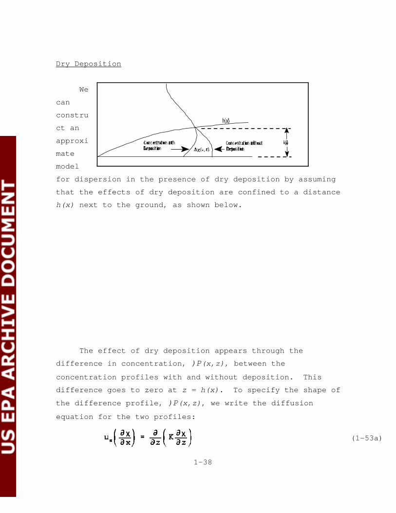
Dry Deposition

We

can

constru

ct an

approxi

mate

model

for dispersion in the presence of dry deposition by assuming

that the effects of dry deposition are confined to a distance

h(x) next to the ground, as shown below.

The effect of dry deposition appears through the

difference in concentration, )P(x,z), between the

concentration profiles with and without deposition. This

difference goes to zero at z = h(x). To specify the shape of

the difference profile, )P(x,z), we write the diffusion

equation for the two profiles:

1-39

(1-53b)

(1-54)

(1-55)

(1-56)

(1-57a)

and

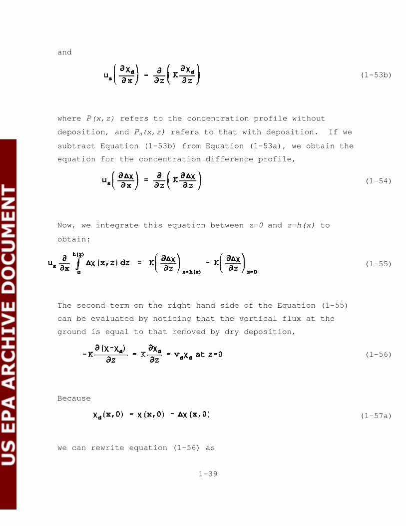
where P(x,z) refers to the concentration profile without

deposition, and Pd(x,z) refers to that with deposition. If we

subtract Equation (1-53b) from Equation (1-53a), we obtain the

equation for the concentration difference profile,

Now, we integrate this equation between z=0 and z=h(x) to

obtain:

The second term on the right hand side of the Equation (1-55)

can be evaluated by noticing that the vertical flux at the

ground is equal to that removed by dry deposition,

Because

we can rewrite equation (1-56) as

1-40

(1-57b)

(1-58)

(1-59)

(1-60)

We can always define h(x) so that the gradient of the

concentration difference profile is zero at z=h(x); then, the

first term on the right hand side of Equation (1-55)

disappears. A concentration difference profile that meets the

zero gradient assumption at z=h(x) is

If we substitute Equation (1-58) into Equation (1-55) and

integrate, we find

Integrating Equation (1-59) yields,

1-41

(1-61)

(1-61a)

All else being equal, Equation (1-60) can be re-written by

replacing the concentrations (P and Pd) with the corresponding

vertical terms (V and Vd) as follows:

From the solution of Equation (1-61), Vd can be calculated as

follows:

1-42

(1-62)

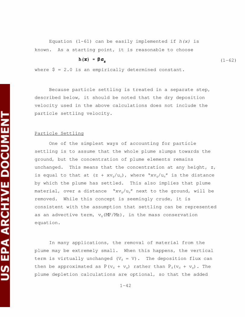
Equation (1-61) can be easily implemented if h(x) is

known. As a starting point, it is reasonable to choose

where $ = 2.0 is an empirically determined constant.

Because particle settling is treated in a separate step,

described below, it should be noted that the dry deposition

velocity used in the above calculations does not include the

particle settling velocity.

Particle Settling

One of the simplest ways of accounting for particle

settling is to assume that the whole plume slumps towards the

ground, but the concentration of plume elements remains

unchanged. This means that the concentration at any height, z,

is equal to that at (z + xvg/us), where “xvg/us” is the distance

by which the plume has settled. This also implies that plume

material, over a distance “xvg/us” next to the ground, will be

removed. While this concept is seemingly crude, it is

consistent with the assumption that settling can be represented

as an advective term, vg(MP/Mz), in the mass conservation

equation.

In many applications, the removal of material from the

plume may be extremely small. When this happens, the vertical

term is virtually unchanged (Vd = V). The deposition flux can

then be approximated as P(vd + vg) rather than Pd(vd + vg). The

plume depletion calculations are optional, so that the added

1-43

(1-63)

(1-64)

expense of computing Pd can be avoided. Not considering the

effects of dry depletion results in conservative estimates of

both concentration and deposition, since material deposited on

the surface is not removed from the plume.

1.1.7 The Decay Term (D)

The Decay Term in Equation (1-1) is a simple method of

accounting for pollutant removal by physical or chemical

processes. It is of the form:

where:

R = the decay coefficient (s-1) (a value of zero meansdecay is not considered)

x = downwind distance (m)

For example, if T1/2 is the pollutant half life in seconds, the

user can obtain R from the relationship:

The default value for R is zero. That is, decay is not

considered in the model calculations unless R is specified.

1-44

However, a decay half life of 4 hours (R = 0.0000481 s-1) is

automatically assigned for SO2 when modeled in the urban mode.

1.2 NON-POINT SOURCE EMISSIONS

1.2.1 General

The ISC models include algorithms to model volume, area

and open-pit sources, in addition to point sources. These non-

point source options of the ISC models are used to simulate the

effects of emissions from a wide variety of industrial sources.

In general, the ISC volume source model is used to simulate the

effects of emissions from sources such as building roof

monitors and line sources (for example, conveyor belts and rail

lines). The ISC area source model is used to simulate the

effects of fugitive emissions from sources such as storage

piles and slag dumps. The ISC open pit source model is used to

simulate fugitive emissions from below-grade open pits, such as

surface coal mines or stone quarries.

1.2.2 The Short-Term Volume Source Model

The ISC models use a virtual point source algorithm to

model the effects of volume sources, which means that an

imaginary or virtual point source is located at a certain

distance upwind of the volume source (called the virtual

distance) to account for the initial size of the volume source

plume. Therefore, Equation (1-1) is also used to calculate

concentrations produced by volume source emissions.

1-45

There are two types of volume sources: surface-based

sources, which may also be modeled as area sources, and

elevated sources. An example of a surface-based source is a

surface rail line. The effective emission height he for a

surface-based source is usually set equal to zero. An example

of an elevated source is an elevated rail line with an

effective emission height he set equal to the height of the

rail line. If the volume source is elevated, the user assigns

the effective emission height he, i.e., there is no plume rise

associated with volume sources. The user also assigns initial

lateral (Fyo) and vertical (Fzo) dimensions for the volume

source. Lateral (xy) and vertical (xz) virtual distances are

added to the actual downwind distance x for the Fy and Fz

calculations. The virtual distances are calculated from

solutions to the sigma equations as is done for point sources

with building downwash.

The volume source model is used to simulate the effects of

emissions from sources such as building roof monitors and for

line sources (for example, conveyor belts and rail lines). The

north-south and east-west dimensions of each volume source used

in the model must be the same. Table 1-6 summarizes the

general procedures suggested for estimating initial lateral

(Fyo) and vertical (Fzo) dimensions for single volume sources

and for multiple volume sources used to represent a line

source. In the case of a long and narrow line source such as a

rail line, it may not be practical to divide the source into N

volume sources, where N is given by the length of the line

source divided by its width. The user can obtain an

approximate representation of the line source by placing a

smaller number of volume sources at equal intervals along the

line source, as shown in Figure 1-8. In general, the spacing

1-46

between individual volume sources should not be greater than

twice the width of the line source. However, a larger spacing

can be used if the ratio of the minimum source-receptor

separation and the spacing between individual volume sources is

greater than about 3. In these cases, concentrations

calculated using fewer than N volume sources to represent the

line source converge to the concentrations calculated using N

volume sources to represent the line source as long as

sufficient volume sources are used to preserve the horizontal

geometry of the line source.

Figure 1-8 illustrates representations of a curved line

source by multiple volume sources. Emissions from a line

source or narrow volume source represented by multiple volume

sources are divided equally among the individual sources unless

there is a known spatial variation in emissions. Setting the

initial lateral dimension Fyo equal to W/2.15 in Figure 1-8(a)

or 2W/2.15 in Figure 1-8(b) results in overlapping Gaussian

distributions for the individual sources. If the wind

direction is normal to a straight line source that is

represented by multiple volume sources, the initial crosswind

concentration distribution is uniform except at the edges of

the line source. The doubling of Fyo by the user in the

approximate line-source representation in Figure 1-8(b) is

offset by the fact that the emission rates for the individual

volume sources are also doubled by the user.

1-47

TABLE 1-6

SUMMARY OF SUGGESTED PROCEDURES FOR ESTIMATING

INITIAL LATERAL DIMENSIONS Fyo AND

INITIAL VERTICAL DIMENSIONS Fzo FOR VOLUME AND LINE SOURCES

Type of SourceProcedure for Obtaining

Initial Dimension

(a) Initial Lateral Dimensions (Fyo)

Single Volume Source Fyo = length of side dividedby 4.3

Line Source Represented byAdjacent Volume Sources (seeFigure 1-8(a))

Fyo = length of side dividedby 2.15

Line Source Represented bySeparated Volume Sources (seeFigure 1-8(b))

Fyo = center to centerdistance divided by2.15

(b) Initial Vertical Dimensions (Fzo)

Surface-Based Source (he - 0) Fzo = vertical dimension ofsource divided by 2.15

Elevated Source (he > 0) on orAdjacent to a Building

Fzo = building heightdivided by 2.15

Elevated Source (he > 0) noton or Adjacent to a Building

Fzo = vertical dimension ofsource divided by 4.3

1-48

(1-65)

1.2.3 The Short-Term Area Source Model

The ISC Short Term area source model is based on a

numerical integration over the area in the upwind and crosswind

directions of the Gaussian point source plume formula given in

Equation (1-1). Individual area sources may be represented as

rectangles with aspect ratios (length/width) of up to 10 to 1.

In addition, the rectangles may be rotated relative to a north-

south and east-west orientation. As shown by Figure 1-9, the

effects of an irregularly shaped area can be simulated by

dividing the area source into multiple areas. Note that the

size and shape of the individual area sources in Figure 1-9

varies; the only requirement is that each area source must be a

rectangle. As a result, an irregular area source can be

represented by a smaller number of area sources than if each

area had to be a square shape. Because of the flexibility in

specifying elongated area sources with the Short Term model, up

to an aspect ratio of about 10 to 1, the ISCST area source

algorithm may also be useful for modeling certain types of line

sources.

The ground-level concentration at a receptor located

downwind of all or a portion of the source area is given by a

double integral in the upwind (x) and crosswind (y) directions

as:

where:

1-49

QA = area source emission rate (mass per unit area perunit time)

K = units scaling coefficient (Equation (1-1))

V = vertical term (see Section 1.1.6)

D = decay term as a function of x (see Section 1.1.7)

The Vertical Term is given by Equation (1-50) or Equation

(1-54) with the effective emission height, he, being the

physical release height assigned by the user. In general, he

should be set equal to the physical height of the source of

emissions above local terrain height. For example, the

emission height he of a slag dump is the physical height of the

slag dump.

Since the ISCST algorithm estimates the integral over the

area upwind of the receptor location, receptors may be located

within the area itself, downwind of the area, or adjacent to

the area. However, since Fz goes to 0 as the downwind distance

goes to 0 (see Section 1.1.5.1), the plume function is infinite

for a downwind receptor distance of 0. To avoid this

singularity in evaluating the plume function, the model

arbitrarily sets the plume function to 0 when the receptor

distance is less than 1 meter. As a result, the area source

algorithm will not provide reliable results for receptors

located within or adjacent to very small areas, with dimensions

on the order of a few meters across. In these cases, the

receptor should be placed at least 1 meter outside of the area.

1-50

(1-66)

(1-67)

In Equation (1-65), the integral in the lateral (i.e.,

crosswind or y) direction is solved analytically as follows:

where erfc is the complementary error function.

In Equation (1-65), the integral in the longitudinal

(i.e., upwind or x) direction is approximated using numerical

methods based on Press, et al (1986). Specifically, the ISCST

model estimates the value of the integral, I, as a weighted

average of previous estimates, using a scaled down

extrapolation as follows:

where the integral term refers to the integral of the plume

function in the upwind direction, and IN and I2N refer to

successive estimates of the integral using a trapezoidal

approximation with N intervals and 2N intervals. The number of

intervals is doubled on successive trapezoidal estimates of the

integral. The ISCST model also performs a Romberg integration

by treating the sequence Ik as a polynomial in k. The Romberg

integration technique is described in detail in Section 4.3 of

Press, et al (1986). The ISCST model uses a set of three

criteria to determine whether the process of integrating in the

upwind direction has "converged." The calculation process will

be considered to have converged, and the most recent estimate

of the integral used, if any of the following conditions is

true:

1-51

1) if the number of "halving intervals" (N) in thetrapezoidal approximation of the integral has reached10, where the number of individual elements in theapproximation is given by 1 + 2N-1 = 513 for N of 10;

2) if the extrapolated estimate of the real integral(Romberg approximation) has converged to within atolerance of 0.0001 (i.e., 0.01 percent), and atleast 4 halving intervals have been completed; or

3) if the extrapolated estimate of the real integral isless than 1.0E-10, and at least 4 halving intervalshave been completed.

The first condition essentially puts a time limit on the

integration process, the second condition checks for the

accuracy of the estimate of the integral, and the third

condition places a lower threshold limit on the value of the

integral. The result of these numerical methods is an estimate

of the full integral that is essentially equivalent to, but

much more efficient than, the method of estimating the integral

as a series of line sources, such as the method used by the PAL

2.0 model (Petersen and Rumsey, 1987).

1-52

1.2.4 The Short-Term Open Pit Source Model

The ISC open pit source model is used to estimate impacts

for particulate emissions originating from a below-grade open

pit, such as a surface coal mine or a stone quarry. The ISC

models allow the open pit source to be characterized by a

rectangular shape with an aspect ratio (length/width) of up to

10 to 1. The rectangular pit may also be rotated relative to a

north-south and east-west orientation. Since the open pit

model does not apply to receptors located within the boundary

of the pit, the concentration at those receptors will be set to

zero by the ISC models.

The model accounts for partial retention of emissions

within the pit by calculating an escape fraction for each

particle size category. The variations in escape fractions

across particle sizes result in a modified distribution of mass

escaping from the pit. Fluid modeling has shown that within-

pit emissions have a tendency to escape from the upwind side of

the pit. The open pit algorithm simulates the escaping pit

emissions by using an effective rectangular area source using

the ISC area source algorithm described in Section 1.2.3. The

shape, size and location of the effective area source varies

with the wind direction and the relative depth of the pit.

Because the shape and location of the effective area source

varies with wind direction, a single open pit source should not

be subdivided into multiple pit sources.

The escape fraction for each particle size catagory, gi,

is calculated as follows:

1-53

(1-68)

(1-69)

where:

vg = is the gravitational settling velocity (m/s),

Ur = is the approach wind speed at 10m (m/s),

" = is the proportionality constant in therelationship between flux from the pit and theproduct of Ur and concentration in the pit(Thompson, 1994).

The gravitational settling velocity, vg, is computed as

described in Section 1.3.2 for each particle size category.

Thompson (1994) used laboratory measurements of pollutant

residence times in a variety of pit shapes typical of actual

mines and determined that a single value of " = 0.029 worked

well for all pits studied.

The adjusted emission rate (Qi) for each particle size

category is then computed as:

where Q is the total emission rate (for all particles) within

the pit, Ni is the original mass fraction for the given size

category, and g is the escape fraction calculated from

Equation (1-68). The adjusted total emission rate (for all

particles escaping the pit), Qa, is the sum of the Qi for all

particle categories calculated from Equation 1-69. The mass

1-54

(1-70)

(1-71)

fractions (of particles escaping the pit), Nai, for each

category is:

Because of particle settling within the pit, the distribution

of mass escaping the pit is different than that emitted within

the pit. The adjusted total particulate emission rate, Qa, and

the adjusted mass fractions, Nai, reflect this change, and it

is these adjusted values that are used for modeling the open

pit emissions.

The following describes the specification of the location,

dimensions and adjusted emissions for the effective area source

used for modeling open pit emissions. Consider an arbitrary

rectangular-shaped pit with an arbitrary wind direction as

shown in Figure 1-10. The steps that the model uses for

determining the effective area source are as follows:

1. Determine the upwind sides of the pit based on thewind direction.

2. Compute the along wind length of the pit (R) based onthe wind direction and the pit geometry . R variesbetween the lengths of the two sides of therectangular pit as follows:

where L is the long axis and W is the short axis ofthe pit, and 2 is the wind direction relative to thelong axis (L) of the pit (therefore 2 varies between0° and 90°). Note that with this formulation and a

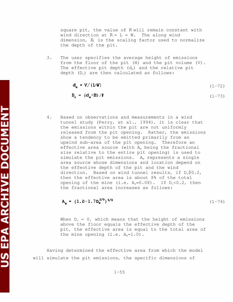
1-55

(1-72)

(1-73)

(1-74)

square pit, the value of R will remain constant withwind direction at R = L = W. The along winddimension, R, is the scaling factor used to normalizethe depth of the pit.

3. The user specifies the average height of emissionsfrom the floor of the pit (H) and the pit volume (V). The effective pit depth (de) and the relative pitdepth (Dr) are then calculated as follows:

4. Based on observations and measurements in a windtunnel study (Perry, et al., 1994), it is clear thatthe emissions within the pit are not uniformlyreleased from the pit opening. Rather, the emissionsshow a tendency to be emitted primarily from anupwind sub-area of the pit opening. Therefore aneffective area source (with Ae being the fractionalsize relative to the entire pit opening) is used tosimulate the pit emissions. Ae represents a singlearea source whose dimensions and location depend onthe effective depth of the pit and the winddirection. Based on wind tunnel results, if Dr$0.2,then the effective area is about 8% of the totalopening of the mine (i.e. Ae=0.08). If Dr<0.2, thenthe fractional area increases as follows:

When Dr = 0, which means that the height of emissionsabove the floor equals the effective depth of thepit, the effective area is equal to the total area ofthe mine opening (i.e. Ae=1.0).

Having determined the effective area from which the model

will simulate the pit emissions, the specific dimensions of

1-56

(1-75)

(1-76)

(1-77)

this effective rectangular area are calculated as a function of

2 such that (see Figure 1-10):

and

Note that in equations 1-75 and 1-76, W is defined as the short

dimension of the pit and L is the long dimension; AW is the

dimension of the effective area aligned with the short side of

the pit and AL is the dimension of the effective area aligned

with the long side of the pit (see Figure 1-10). The

dimensions AW and AL are used by the model to define the shape

of the effective area for input to the area source algorithm

described in Section 1.2.3.

The emission rate, Qe, for the effective area is such that

where Qa is the emission rate per unit area (from the pit after

adjustment for escape fraction) if the emissions were uniformly

released from the actual pit opening (with an area of L@W).

That is, if the effective area is one-third of the total area,

then the emission rate (per unit area) used for the effective

area is three times that from the full area.

1-57

(1-78)

Because of the high level of turbulence in the mine, the

pollutant is initially mixed prior to exiting the pit.

Therefore some initial vertical dispersion is included to

represent this in the effective area source. Using the

effective pit depth, de, as the representative dimension over

which the pollutant is vertically mixed in the pit, the initial

vertical dispersion value, Fzo, is equal to de/4.3. Note that

4.3@Fzo represents about 90% of a Gaussian plume (in the

vertical), so that the mixing in the pit is assumed to

approximately equal the mixing in a plume.

Therefore, for the effective area source representing the

pit emissions, the initial dispersion is included with ambient

dispersion as:

For receptors close to the pit, the initial dispersion value

can be particularly important.

Once the model has determined the characteristics of the

effective area used to model pit emissions for a particular

hour, the area source algorithm described in Section 1.2.3 is

used to calculate the concentration or deposition flux values

at the receptors being modeled.

1.3 THE ISC SHORT-TERM DRY DEPOSITION MODEL

1.3.1 General

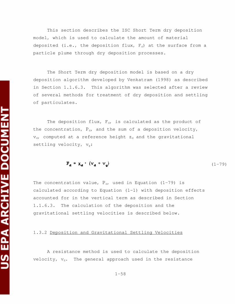
1-58

(1-79)

This section describes the ISC Short Term dry deposition

model, which is used to calculate the amount of material

deposited (i.e., the deposition flux, Fd) at the surface from a

particle plume through dry deposition processes.

The Short Term dry deposition model is based on a dry

deposition algorithm developed by Venkatram (1998) as described

in Section 1.1.6.3. This algorithm was selected after a review

of several methods for treatment of dry deposition and settling

of particulates.

The deposition flux, Fd, is calculated as the product of

the concentration, Pd, and the sum of a deposition velocity,

vd, computed at a reference height zd and the gravitational

settling velocity, vg:

The concentration value, Pd, used in Equation (1-79) is

calculated according to Equation (1-1) with deposition effects

accounted for in the vertical term as described in Section

1.1.6.3. The calculation of the deposition and the

gravitational settling velocities is described below.

1.3.2 Deposition and Gravitational Settling Velocities

A resistance method is used to calculate the deposition

velocity, vd. The general approach used in the resistance

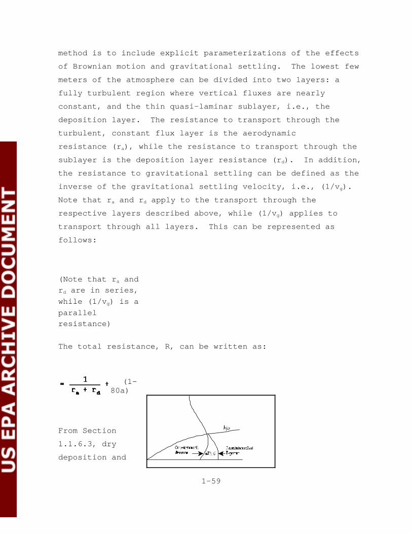
1-59

(1-80a)

method is to include explicit parameterizations of the effects

of Brownian motion and gravitational settling. The lowest few

meters of the atmosphere can be divided into two layers: a

fully turbulent region where vertical fluxes are nearly

constant, and the thin quasi-laminar sublayer, i.e., the

deposition layer. The resistance to transport through the

turbulent, constant flux layer is the aerodynamic

resistance (ra), while the resistance to transport through the

sublayer is the deposition layer resistance (rd). In addition,

the resistance to gravitational settling can be defined as the

inverse of the gravitational settling velocity, i.e., (1/vg).

Note that ra and rd apply to the transport through the

respective layers described above, while (1/vg) applies to

transport through all layers. This can be represented as

follows:

(Note that ra andrd are in series,

while (1/vg) is a

parallelresistance)

The total resistance, R, can be written as:

From Section

1.1.6.3, dry

deposition and

1-60

(1-80b)

(1-81)

(1-82)

gravitational settling are treated as independent processes

wherein the dry deposition is only dependent upon the

resistances to transport through the various layers, and

gravitational settling is only dependent upon vg. Therefore,

the deposition velocity (vd) is defined as the inverse of the

sum of resistances to pollutant transfer through various

layers:

where, vd = the deposition velocity (cm/s),

ra = the aerodynamic resistance (s/cm), and,

rd = the deposition layer resistance (s/cm).

It is usually assumed that the eddy diffusivity for mass

transfer within the turbulent, constant flux layer is similar

to that for heat. The atmospheric resistance formulation is

based on Byun and Dennis (1995):

stable (L > 0):

unstable (L < 0):

1-61

(1-83)

where, u* = the surface friction velocity (cm/s),

k = the von Karman constant (0.4),

z = the height above ground (m),

L = the Monin-Obukhov length (m),

zd = deposition reference height (m), and

zo = the surface roughness length (m).

The coefficients used in the atmospheric resistance formulation

are those suggested by Dyer (1974). A minimum value for L of

1.0m is used for rural locations. Recommended minimum values

for urban areas are provided in the user's guides for the

meteorological preprocessor programs PCRAMMET and MPRM.

The deposition layer resistance term is parameterized as

per the approach used by Pleim et al. (1984) as follows:

where, Sc = the Schmidt number (Sc = L/DB)

(dimensionless),

L = the viscosity of air (ï 0.15 cm2/s),

DB = the Brownian diffusivity (cm2/s) of the

pollutant in air,

1-62

(1-84)

(1-85)

(1-86)

The first term of Eqn. (1-83), involving the Schmidt

number, parameterizes the effects of Brownian motion. The

Brownian diffusivity of the pollutant (in cm2/s) is computed

from the following relationship:

where, Ta = air temperature (°K),

dp = the particle diameter (:m),

SCF = the slip correction factor, which is computed

as:

and, x2, a1, a2, a3 are constants with values of 6.5 x 10-6,

1.257, 0.4, and 0.55 x 10-4, respectively.

The gravitational settling velocity, vg (cm/s), is

calculated as:

where, D = the particle density (g/cm3),

DAIR = the air density (ï 1.2 x 10-3 g/cm3),

g = the acceleration due to gravity (981 cm/s2),

1-63

: = the absolute viscosity of air (ï 1.81 x 10-4

g/cm/s), and

c2 = air units conversion constant (1 x 10-8

cm2/:m2).

The deposition algorithm also allows a small adjustment to

the deposition rates to account for possible phoretic effects.

Some examples of phoretic effects (Hicks, 1982) are:

THERMOPHORESIS: Particles close to a hot surface experience aforce directed away from the surface because, on theaverage, the air molecules impacting on the side of theparticle facing the surface are hotter and more energetic.

DIFFUSIOPHORESIS: Close to an evaporating surface, a particleis more likely to be impacted by water molecules on theside of the particle facing the surface. Since the watermolecules have a lower molecular weight than the averageair molecule, there is a net force toward the surface,which results in a small enhancement of the depositionvelocity of the particle.

A second effect is that the impaction of new water vapormolecules at an evaporating surface displaces a certainvolume of air. For example, 18 g of water vaporevaporating from 1 m2 will displace 22.4 liters of air atstandard temperature and pressure (STP) conditions (Hicks,1982). This effect is called Stefan flow. The Stefanflow effect tends to reduce deposition fluxes from anevaporating surface. Conversely, deposition fluxes to asurface experiencing condensation will be enhanced.

ELECTROPHORESIS: Attractive electrical forces have thepotential to assist the transport of small particlesthrough the quasi-laminar deposition layer, and thus couldincrease the deposition velocity in situations with highlocal field strengths. However, Hicks (1982) suggeststhis effect is likely to be small in most naturalcircumstances.

1-64

Phoretic and Stefan flow effects are generally small.

However, for particles in the range of 0.1 - 1.0 :m diameter,

which have low deposition velocities, these effects may not

always be negligible. Therefore, the ability to specify a

phoretic term to the deposition velocity is added (i.e., vdN =

vd + vd(phor), where vdN is the modified deposition velocity and

vd(phor) is the phoretic term).

Although the magnitude and sign of vd(phor) will vary, a

small, constant value of + 0.01 cm/s is used in the present

implementation of the model to represent combined phoretic

effects.

In addition to the mass mean diameters (microns), particle

densities (gm/cm3), and the mass fractions for each particle

size category being modeled, the dry deposition model also

requires surface roughness length (cm), friction velocity

(m/s), and Monin-Obukhov length (m). The surface roughness

length is specified by the user, and the meteorological

preprocessor (PCRAMMET or MPRM) calculates the friction

velocity and Monin-Obukhov length for input to the model.

1.3.3 Point and Volume Source Emissions

As stated in Equation (1-79), deposition is modeled as the

product of the near-surface concentration (from Equation (1-1))

times the deposition velocity (from Equation (1-80b)).

Therefore, the vertical term given in Equation (1-61) that is

used to obtain the concentration at height z, subject to

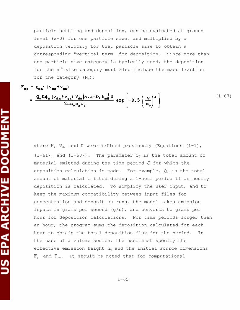
1-65

(1-87)

particle settling and deposition, can be evaluated at ground

level (z=0) for one particle size, and multiplied by a

deposition velocity for that particle size to obtain a

corresponding "vertical term" for deposition. Since more than

one particle size category is typically used, the deposition

for the nth size category must also include the mass fraction

for the category (Nn):

where K, Vd, and D were defined previously (Equations (1-1),

(1-61), and (1-63)). The parameter QJ is the total amount of

material emitted during the time period J for which the

deposition calculation is made. For example, QJ is the total

amount of material emitted during a 1-hour period if an hourly

deposition is calculated. To simplify the user input, and to

keep the maximum compatibility between input files for

concentration and deposition runs, the model takes emission

inputs in grams per second (g/s), and converts to grams per

hour for deposition calculations. For time periods longer than

an hour, the program sums the deposition calculated for each

hour to obtain the total deposition flux for the period. In

the case of a volume source, the user must specify the

effective emission height he and the initial source dimensions

Fyo and Fzo. It should be noted that for computational

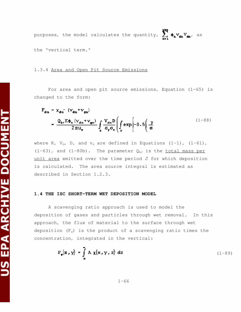
1-66

(1-88)

(1-89)

purposes, the model calculates the quantity, , as

the "vertical term."

1.3.4 Area and Open Pit Source Emissions

For area and open pit source emissions, Equation (1-65) is

changed to the form:

where K, Vd, D, and vd are defined in Equations (1-1), (1-61),

(1-63), and (1-80b). The parameter QAJ is the total mass per

unit area emitted over the time period J for which deposition

is calculated. The area source integral is estimated as

described in Section 1.2.3.

1.4 THE ISC SHORT-TERM WET DEPOSITION MODEL

A scavenging ratio approach is used to model the

deposition of gases and particles through wet removal. In this

approach, the flux of material to the surface through wet

deposition (Fw) is the product of a scavenging ratio times the

concentration, integrated in the vertical:

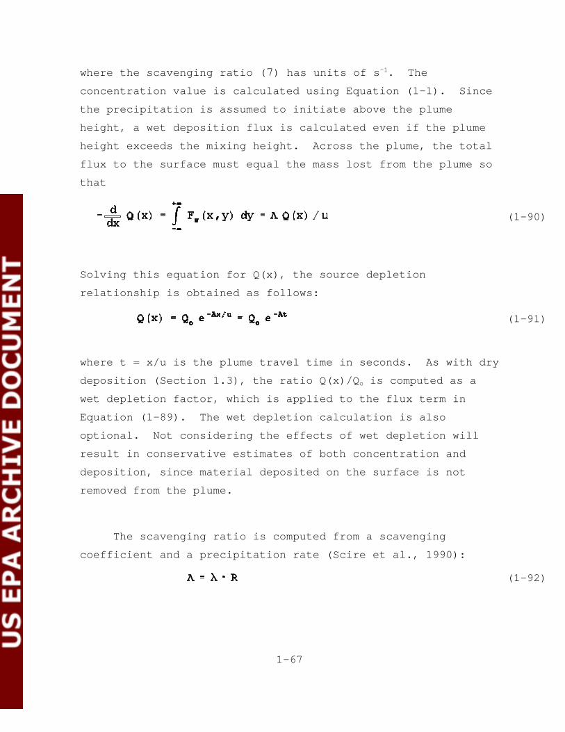
1-67

(1-90)

(1-91)

(1-92)

where the scavenging ratio (7) has units of s-1. The

concentration value is calculated using Equation (1-1). Since

the precipitation is assumed to initiate above the plume

height, a wet deposition flux is calculated even if the plume

height exceeds the mixing height. Across the plume, the total

flux to the surface must equal the mass lost from the plume so

that

Solving this equation for Q(x), the source depletion

relationship is obtained as follows:

where t = x/u is the plume travel time in seconds. As with dry

deposition (Section 1.3), the ratio Q(x)/Qo is computed as a

wet depletion factor, which is applied to the flux term in

Equation (1-89). The wet depletion calculation is also

optional. Not considering the effects of wet depletion will

result in conservative estimates of both concentration and

deposition, since material deposited on the surface is not

removed from the plume.

The scavenging ratio is computed from a scavenging

coefficient and a precipitation rate (Scire et al., 1990):

1-68

where the coefficient 8 has units (s-mm/hr)-1, and the

precipitation rate R has units (mm/hr). The scavenging

coefficient depends on the characteristics of the pollutant

(e.g., solubility and reactivity for gases, size distribution

for particles) as well as the nature of the precipitation

(e.g., liquid or frozen). Jindal and Heinold (1991) have

analyzed particle scavenging data reported by Radke et al.

(1980), and found that the linear relationship of Equation

(1-90) provides a better fit to the data than the non-linear

assumption 7 = 8Rb. Furthermore, they report best-fit values

for 8 as a function of particle size. These values of the

scavenging rate coefficient are displayed in Figure 1-11.

Although the largest particle size included in the study is 10

:m, the authors suggest that 8 should reach a plateau beyond

10 :m, as shown in Figure 1-11. The scavenging rate

coefficients for frozen precipitation are expected to be

reduced to about 1/3 of the values in Figure 1-11 based on data

for sulfate and nitrate (Scire et al., 1990). The scavenging

rate coefficients are input to the model by the user.

The wet deposition algorithm requires precipitation type

(liquid or solid) and precipitation rate, which is prepared for

input to the model through the meteorological preprocessor

programs (PCRAMMET or MPRM).

1-69

1.5 ISC COMPLEX TERRAIN SCREENING ALGORITHMS

The Short Term model uses a steady-state, sector-averaged

Gaussian plume equation for applications in complex terrain

(i.e., terrain above stack or release height). Terrain below

release height is referred to as simple terrain; receptors

located in simple terrain are modeled with the point source

model described in Section 1.1. The sector average approach

used in complex terrain implies that the lateral (crosswind)

distribution of concentrations is uniform across a 22.5 degree

sector. The complex terrain screening algorithms apply only to

point source and volume source emissions; area source and open

pit emission sources are excluded. The complex terrain point

source model, which is based on the COMPLEX1 model, is

described below. The description parallels the discussion for

the simple terrain algorithm in Section 1.1, and includes the

basic Gaussian sector-average equation, the plume rise

formulas, and the formulas used for determining dispersion

parameters.

1.5.1 The Gaussian Sector Average Equation

The Short Term complex terrain screening algorithm for

stacks uses the steady-state, sector-averaged Gaussian plume

equation for a continuous elevated source. As with the simple

terrain algorithm described in Section 1.1, the origin of the

source's coordinate system is placed at the ground surface at

the base of the stack for each source and each hour. The x

axis is positive in the downwind direction, the y axis is

crosswind (normal) to the x axis and the z axis extends

1-70

(1-93)

vertically. The fixed receptor locations are converted to each

source's coordinate system for each hourly concentration

calculation. Since the concentrations are uniform across a

22.5 degree sector, the complex terrain algorithms use the

radial distance between source and receptor instead of downwind

distance. The calculation of the downwind, crosswind and

radial distances is described in Section 1.5.2. The hourly

concentrations calculated for each source at each receptor are

summed to obtain the total concentration produced at each

receptor by the combined source emissions.

For a Gaussian, sector-averaged plume, the hourly

concentration at downwind distance x (meters) and crosswind

distance y (meters) is given by:

where:

Q = pollutant emission rate (mass per unit time),

K = units scaling coefficient (see Equation (1-1))

)2' = the sector width in radians (=0.3927)

R = radial distance from the point source to thereceptor = [(x+xy)2 + y2]1/2 (m)

x = downwind distance from source center toreceptor, measured along the plume axis (m)

y = lateral distance from the plume axis to thereceptor (m)

1-71

xy = lateral virtual distance for volume sources (seeEquation (1-35)), equals zero for point sources(m)

us = mean wind speed (m/sec) at stack height

Fz = standard deviation of the vertical concentrationdistribution (m)

V = the Vertical Term (see Section 1.1.6)

D = the Decay Term (see Section 1.1.7)

CORR = the attenuation correction factor for receptorsabove the plume centerline height (see Section1.5.8)

Equation (1-93) includes a Vertical Term, a Decay Term,

and a vertical dispersion term (Fz). The Vertical Term

includes the effects of source elevation, receptor elevation,

plume rise, limited vertical mixing, gravitational settling and

dry deposition.

1.5.2 Downwind, Crosswind and Radial Distances

The calculation of downwind and crosswind distances is

described in Section 1.1.2. Since the complex terrain

algorithms in ISC are based on a sector average, the radial

distance is used in calculating the plume rise (see Section

1.5.4) and dispersion parameters (see Section 1.5.5). The

radial distance is calculated as R = [x2 + y2]1/2, where x is the

downwind distance and y is the crosswind distance described in

Section 1.1.2.

1-72

1.5.3 Wind Speed Profile

See the discussion given in Section 1.1.3.

1.5.4 Plume Rise Formulas

The complex terrain algorithm in ISC uses the Briggs plume

rise equations described in Section 1.1.4. For distances less

than the distance to final rise, the complex terrain algorithm

uses the distance-dependent plume height (based on the radial

distance) as described in Section 1.1.4.10. Since the complex

terrain algorithm does not incorporate the effects of building

downwash, the Schulman-Scire plume rise described in Section

1.1.4.11 is not used for complex terrain modeling. The plume

height is used in the calculation of the Vertical Term

described in Section 1.5.6.

1-73

1.5.5 The Dispersion Parameters

The dispersion parameters used in the complex terrain

algorithms of ISC are the same as the point source dispersion

parameters for the simple terrain algorithms described in

Section 1.1.5.1, except that the radial distance is used

instead of the downwind distance. Since the lateral

distribution of the plume in complex terrain is determined by

the sector average approach, the complex terrain algorithm does

not use the lateral dispersion parameter, Fy. The procedure to

account for buoyancy-induced dispersion in the complex terrain

algorithm only affects the vertical dispersion term (see

Equation 1-48). Since the complex terrain algorithm does not

incorporate the effects of building downwash, the enhanced

dispersion parameters and virtual distances do not apply.

1.5.6 The Vertical Term

The Vertical Term used in the complex terrain algorithm in

ISC is the same as described in Section 1.1.6 for the simple

terrain algorithm, except that the plume height and dispersion

parameter input to the vertical term are based on the radial

distance, as described above, and that the adjustment of plume

height for terrain above stack base is different, as described

in Section 1.5.6.1.

1-74

(1-94)

1.5.6.1 The Vertical Term in Complex Terrain.

The ISC complex terrain algorithm makes the following

assumption about plume behavior in complex terrain:

• The plume axis remains at the plume stabilizationheight above mean sea level as it passes over complexterrain for stable conditions (categories E and F), anduses a "half-height" correction factor for unstable andneutral conditions (categories A - D).

• The plume centerline height is never less than 10 mabove the ground level in complex terrain.

• The mixing height is terrain following, i.e, the mixingheight above ground at the receptor location is assumedto be the same as the height above ground at the sourcelocation.

• The wind speed is a function of height above thesurface (see Equation (1-6)).

Thus, a modified plume stabilization height he' is

substituted for the effective stack height he in the Vertical

Term given by Equation (1-50). The effective plume

stabilization height at the point x,y is given by:

where:

he = plume height at point x,y without terrainadjustment, as described in Section 1.5.4 (m)

1-75

Ht = z*(x,y) - zs = terrain height of the receptorlocation above the base of the stack (m)

z*(x,y) = height above mean sea level of terrain at thereceptor location (x,y) (m)

zs = height above mean sea level of the base of thestack (m)

FT = terrain adjustment factor, which is 0.5 forstability categories A - D and 0.0 for stabilitycategories E and F.

The effect of the terrain adjustment factor is that the plume

height relative to stack base is deflected upwards by an amount

equal to half of the terrain height as it passes over complex

terrain during unstable and neutral conditions. The plume

height is not deflected by the terrain under stable conditions.

1.5.6.2 The Vertical Term for Particle Deposition

The Vertical Term for particle deposition used in the

complex terrain algorithm in ISC is the same as described in

Section 1.1.6 for the simple terrain algorithm, except that the

plume height and dispersion parameter input to the vertical

term are based on the radial distance, as described above, and

that the adjustment of plume height for terrain above stack

base is different, as described in Section 1.5.6.2.

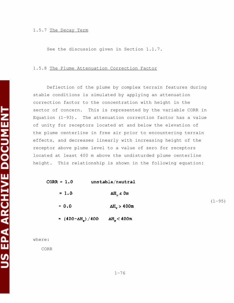
1-76

(1-95)

1.5.7 The Decay Term

See the discussion given in Section 1.1.7.

1.5.8 The Plume Attenuation Correction Factor

Deflection of the plume by complex terrain features during

stable conditions is simulated by applying an attenuation

correction factor to the concentration with height in the

sector of concern. This is represented by the variable CORR in

Equation (1-93). The attenuation correction factor has a value

of unity for receptors located at and below the elevation of

the plume centerline in free air prior to encountering terrain

effects, and decreases linearly with increasing height of the

receptor above plume level to a value of zero for receptors

located at least 400 m above the undisturded plume centerline

height. This relationship is shown in the following equation:

where:

CORR

1-77

= attenuation correction factor, which is between 0and 1

1-78

)Hr

1-79

= height of receptor above undisturbed plume height, includingheight of receptor above local ground (i.e., flagpoleheight)

1.5.9 Wet Deposition in Complex Terrain

See the discussion given in Section 1.4.

1.6 ISC TREATMENT OF INTERMEDIATE TERRAIN

In the ISC Short Term model, intermediate terrain is

defined as terrain that exceeds the height of the release, but

is below the plume centerline height. The plume centerline

height used to define whether a given receptor is on

intermediate terrain is the distance-dependent plume height

calculated for the complex terrain algorithm, before the

terrain adjustment (Section 1.5.6.2) is applied.

If the plume height is equal to or exceeds the terrain

height, then that receptor is defined as complex terrain for

that hour and that source, and the concentration is based on

the complex terrain screening algorithm only. If the terrain

height is below the plume height but exceeds the physical

release height, then that receptor is defined as intermediate

terrain for that hour and source. For intermediate terrain

receptors, concentrations from both the simple terrain

algorithm and the complex terrain algorithm are obtained and

the higher of the two concentrations is used for that hour and

that source. If the terrain height is less than or equal to

the physical release height, then that receptor is defined as

simple terrain, and the concentration is based on the simple

terrain algorithm only.

1-80

For deposition calculations, the intermediate terrain

analysis is first applied to the concentrations at a given

receptor, and the algorithm (simple or complex) that gives the

highest concentration at that receptor is used to calculate the

deposition value.

1-81

FIGURE 1-1.LINEAR DECAY FACTOR, A AS A FUNCTION OF EFFECTIVESTACK HEIGHT, He. A SQUAT BUILDING IS ASSUMED FOR SIMPLICITY.

1-82

1-83

FIGURE 1-2.ILLUSTRATION OF TWO TIERED BUILDING WITH DIFFERENTTIERS DOMINATING DIFFERENT WIND DIRECTIONS

1-84

FIGURE 1-3.THE METHOD OF MULTIPLE PLUME IMAGES USED TO SIMULATEPLUME REFLECTION IN THE ISC2 MODEL

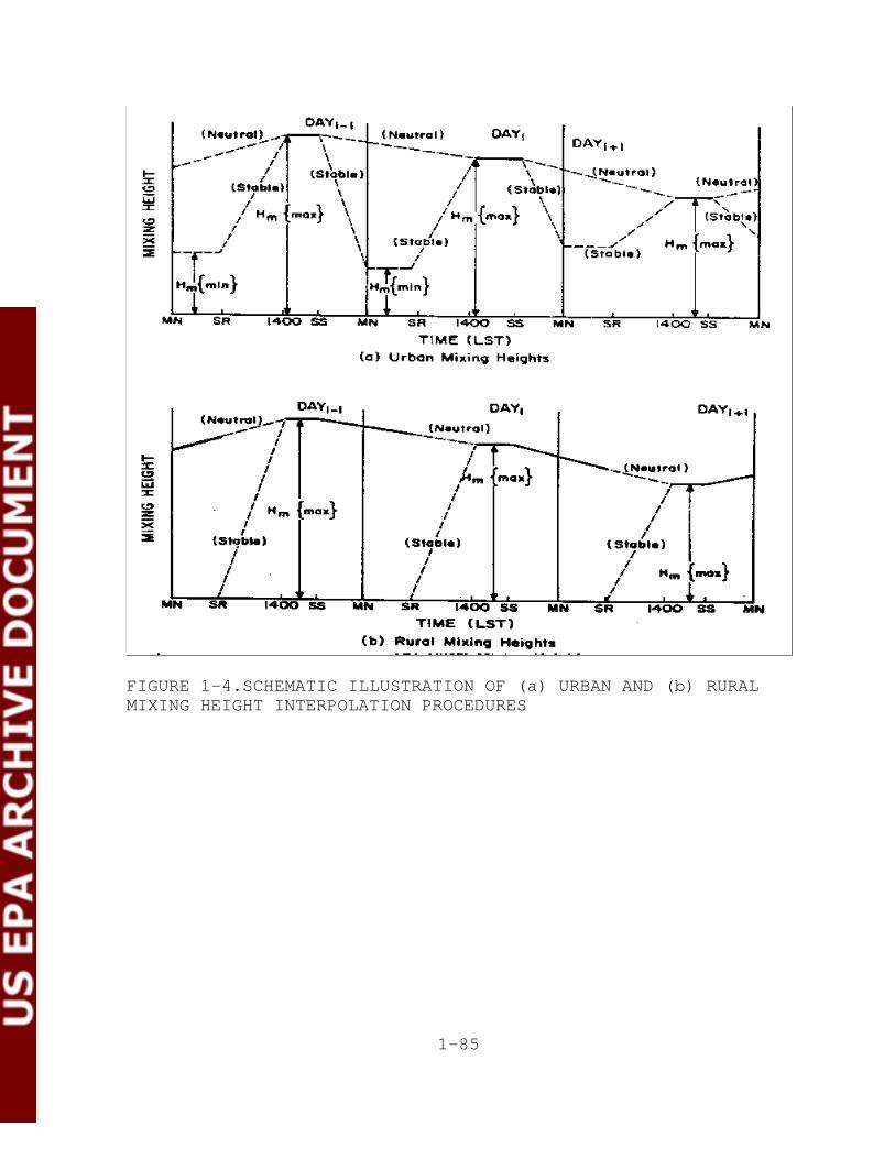
1-85

FIGURE 1-4.SCHEMATIC ILLUSTRATION OF (a) URBAN AND (b) RURALMIXING HEIGHT INTERPOLATION PROCEDURES

1-86

FIGURE 1-5.ILLUSTRATION OF PLUME BEHAVIOR IN ELEVATED TERRAINASSUMED BY THE ISC2 MODEL

1-87

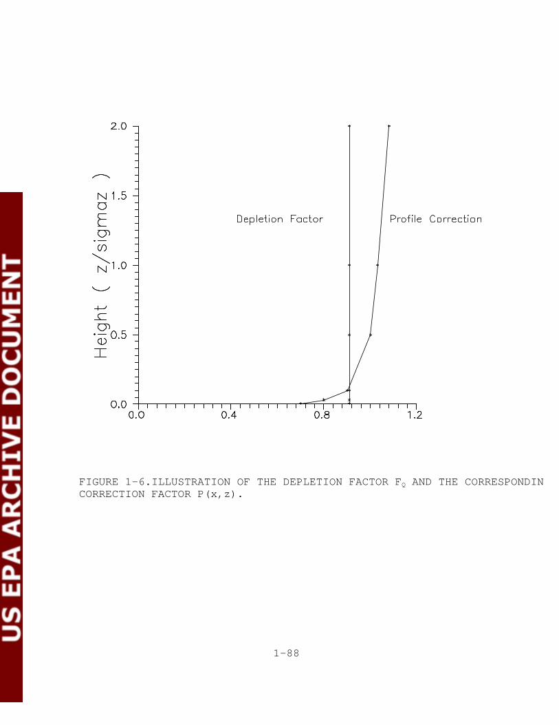
1-88

FIGURE 1-6.ILLUSTRATION OF THE DEPLETION FACTOR FQ AND THE CORRESPONDING PROFILECORRECTION FACTOR P(x,z).

1-89

FIGURE 1-7.VERTICAL PROFILE OF CONCENTRATION BEFORE AND AFTER APPLYING FP(x,z) SHOWN IN

FIGURE 1-6.

1-90

FIGURE 1-8.EXACT AND APPROXIMATE REPRESENTATIONS OF A LINESOURCE BY MULTIPLE VOLUME SOURCES

1-91

1-92

FIGURE 1-9.REPRESENTATION OF AN IRREGULARLY SHAPED AREA SOURCEBY 4 RECTANGULAR AREA SOURCES

1-93

FIGURE 1-10.EFFECTIVE AREA AND ALONGWIND WIDTH FOR AN OPEN PITSOURCE

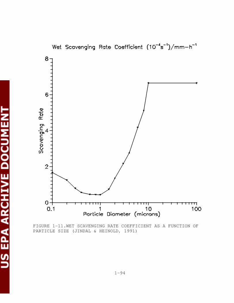
1-94

FIGURE 1-11.WET SCAVENGING RATE COEFFICIENT AS A FUNCTION OFPARTICLE SIZE (JINDAL & HEINOLD, 1991)

2-1

2.0 THE ISC LONG-TERM DISPERSION MODEL EQUATIONS

This section describes the ISC Long-Term model equations.

Where the technical information is the same, this section

refers to the ISC Short-Term model description in Section 1 for

details. The long-term model provides options for modeling the

same types of sources as provided by the short-term model. The

information provided below follows the same order as used for

the short-term model equations.

The ISC long-term model uses input meteorological data

that have been summarized into joint frequencies of occurrence

for particular wind speed classes, wind direction sectors, and

stability categories. These summaries, called STAR summaries

for STability ARray, may include frequency distributions over a

monthly, seasonal or annual basis. The long term model has the

option of calculating concentration or dry deposition values

for each separate STAR summary input and/or for the combined

period covered by all available STAR summaries. Since the wind

direction input is the frequency of occurrence over a sector,

with no information on the distribution of winds within the

sector, the ISC long-term model uses a Gaussian sector-average

plume equation as the basis for modeling pollutant emissions on

a long-term basis.

2-2

(2-1)

2.1 POINT SOURCE EMISSIONS

2.1.1 The Gaussian Sector Average Equation

The ISC long-term model makes the same basic assumption as

the short-term model. In the long-term model, the area

surrounding a continuous source of pollutants is divided into

sectors of equal angular width corresponding to the sectors of

the seasonal and annual frequency distributions of wind

direction, wind speed, and stability. Seasonal or annual

emissions from the source are partitioned among the sectors

according to the frequencies of wind blowing toward the

sectors. The concentration fields calculated for each source

are translated to a common coordinate system (either polar or

Cartesian as specified by the user) and summed to obtain the

total due to all sources.

For a single stack, the mean seasonal concentration is

given by:

where:

K = units scaling coefficient (see Equation (1-1))

Q = pollutant emission rate (mass per unit time),for the ith wind-speed category, the kth

stability category and the lth season

f = frequency of occurrence of the ith wind-speedcategory, the jth wind-direction category andthe kth stability category for the lth season

2-3

(2-2)

)2' = the sector width in radians

R = radial distance from lateral virtual pointsource (for building downwash) to the receptor =[(x+xy)2 + y2]1/2 (m)

x = downwind distance from source center toreceptor, measured along the plume axis (m)

y = lateral distance from the plume axis to thereceptor (m)

xy = lateral virtual distance (see Equation (1-35)),equals zero for point sources without buildingdownwash, and for downwash sources that do notexperience lateral dispersion enhancement (m)

S = a smoothing function similar to that of the AQDM(see Section 2.1.8)

us = mean wind speed (m/sec) at stack height for theith wind-speed category and kth stabilitycategory

Fz = standard deviation of the vertical concentrationdistribution (m) for the kth stability category

V = the Vertical Term for the ith wind-speedcategory, kth stability category and lth season

D = the Decay Term for the ith wind speed categoryand kth stability category

The mean annual concentration at the point (r,2) is

calculated from the seasonal concentrations using the

expression:

2-4

The terms in Equation (2-1) correspond to the terms

discussed in Section 1.1 for the short-term model except

that the parameters are defined for discrete categories of

wind-speed, wind-direction, stability and season. The

various terms are briefly discussed in the following

subsections. In addition to point source emissions, the

ISC long-term concentration model considers emissions from

volume and area sources. These model options are discussed

in Section 2.2. The optional algorithms for calculating

dry deposition are discussed in Section 2.3.

2.1.2 Downwind and Crosswind Distances

See the discussion given in Section 1.1.2.

2.1.3 Wind Speed Profile

See the discussion given in Section 1.1.3.

2.1.4 Plume Rise Formulas

See the discussion given in Section 1.1.4.

2.1.5 The Dispersion Parameters

2.1.5.1 Point Source Dispersion Parameters.

See Section 1.1.5.1 for a discussion of the procedures

use to calculate the standard deviation of the vertical

concentration distribution Fz for point sources (sources

2-5

(2-3)

without initial dimensions). Since the long term model

assumes a uniform lateral distribution across the sector

width, the model does not use the standard deviation of the

lateral dispersion, Fy (except for use with the

Schulman-Scire plume rise formulas described in Section

1.1.4.11).

2.1.5.2 Lateral and Vertical Virtual Distances.

See Section 1.1.5.2 for a discussion of the procedures

used to calculate vertical virtual distances. The lateral

virtual distance is given by:

where ro is the effective source radius in meters. For

volume sources (see Section 2.2.2), the program sets ro

equal to 2.15Fyo, where Fyo is the initial lateral

dimension. For area sources (see Section 2.2.3), the

program sets ro equal to xo/ where xo is the length of

the side of the area source. For plumes affected by

building wakes (see Section 1.1.5.2), the program sets ro

equal to 2.15 Fy' where Fy' is given for squat buildings by

Equation (1-41), (1-42), or (1-43) for downwind distances

between 3 and 10 building heights and for tall buildings by

Equation (1-44) for downwind distances between 3 and 10

building widths. At downwind distances greater than 10

building heights for Equation (1-41), (1-42), or (1-43),

Fy' is held constant at the value of Fy' calculated at a

downwind distance of 10 building heights. Similarly, at

downwind distances greater than 10 building widths for

2-6

Equation (1-44), Fy' is held constant at the value of Fy'

calculated at a downwind distance of 10 building widths.

2.1.5.3 Procedures Used to Account for the Effects ofBuilding Wakes on Effluent Dispersion.

With the exception of the equations used to calculate

the lateral virtual distance, the procedures used to

account for the effects of building wake effects on

effluent dispersion are the same as those outlined in

Section 1.1.5.3 for the short-term model. The calculation

of lateral virtual distances by the long-term model is

discussed in Section 2.1.5.2 above.

2.1.5.4 Procedures Used to Account forBuoyancy-Induced Dispersion.

See the discussion given in Section 1.1.5.4.

2.1.6 The Vertical Term

2.1.6.1 The Vertical Term for Gases and SmallParticulates.

Except for the use of seasons and discrete categories

of wind-speed and stability, the Vertical Term for gases

and small particulates corresponds to the short term

version discussed in Section 1.1.6. The user may assign a

separate mixing height zi to each combination of wind-speed

and stability category for each season.

2-7

(2-4)

As with the Short-Term model, the Vertical Term is

changed to the form:

at downwind distances where the Fz/zi ratio is greater than

or equal to 1.6. Additionally, the ground-level

concentration is set equal to zero if the effective stack

height he exceeds the mixing height zi. As explained in

Section 1.1.6.1, the ISC model currently assumes unlimited

mixing for the E and F stability categories.

2.1.6.2 The Vertical Term in Elevated Terrain.

See the discussion given in Section 1.1.6.2.

2.1.6.3 The Vertical Term for Large Particulates.

Section 1.1.6.3 discusses the differences in the

dispersion of large particulates and the dispersion of

gases and small particulates and provides the guidance on

the use of this option. The Vertical Term for large

particulates is given by Equation (1-53).

2.1.7 The Decay Term

See the discussion given in Section 1.1.7.

2-8

(2-5)

2.1.8 The Smoothing Function

As shown by Equation (2-1), the rectangular

concentration distribution within a given angular sector is

modified by the function S{2} which smooths

discontinuities in the concentration at the boundaries of

adjacent sectors. The centerline concentration in each

sector is unaffected by contribution from adjacent sectors.

At points off the sector centerline, the concentration is a

weighted function of the concentration at the centerline

and the concentration at the centerline of the nearest

adjoining sector. The smoothing function is given by:

where:

2j' = the angle measured in radians from north to thecenterline of the jth wind-direction sector

2' = the angle measured in radians from north to thereceptor point (R, 2) where R, defined above forequation 2-1, is measured from the lateral virtualsource.

2-9

2.2 NON-POINT SOURCE EMISSIONS

2.2.1 General

As explained in Section 1.2.1, the ISC volume, area

and open pit sources are used to simulate the effects of

emissions from a wide variety of industrial sources.

Section 1.2.2 provides a description of the volume source

model, Section 1.2.3 provides a description of the area

source model, and Section 1.2.4 provides a description of

the open pit model. The following subsections give the

volume, area and open pit source equations used by the

long-term model.

2.2.2 The Long-Term Volume Source Model

The ISC Long Term Model uses a virtual point source

algorithm to model the effects of volume sources.

Therefore, Equation (2-1) is also used to calculate

seasonal average ground-level concentrations for volume

source emissions. The user must assign initial lateral

(Fyo) and vertical (Fzo) dimensions and the effective

emission height he. A discussion of the application of the

volume source model is given in Section 1.2.2.

2-10

(2-6a)

(2-6b)

2.2.3 The Long-Term Area Source Model

The ISC Long Term Area Source Model is based on the

numerical integration algorithm for modeling area sources

used by the ISC Short Term model, which is described in

detail in Section 1.2.3. For each combination of wind

speed class, stability category and wind direction sector

in the STAR meteorological frequency summary, the ISC Long

Term model calculates a sector average concentration by

integrating the results from the ISC Short Term area source

algorithm across the sector. A trapezoidal integration is

used, as follows:

where:

Pi = the sector average concentration value for theith sector

S = the sector width

fij = the frequency of occurrence for the jth winddirection in the ith sector

2-11

,(2) = the error term - a criterion of ,(2) < 2percent is used to check for convergence of thesector average calculation

P(2ij) = the concentration value, based on the numericalintegration algorithm using Equation (1-58) forthe jth wind direction in the ith sector

2ij = the jth wind direction in the ith sector, j = 1and N correspond to the two boundaries of thesector.

The application of Equation (2-6a) to calculate the sector

average concentration from area sources is an iterative

process. Calculations using the ISC Short Term algorithm

(Equation (1-58)) are initially made for three wind

directions, corresponding to the two boundaries of the

sector and the centerline direction. The algorithm then

calculates the concentration for wind directions midway

between the three directions, for a total of five

directions, and calculates the error term. If the error is

less than 2 percent, then the concentration based on five

directions is used to represent the sector average,

otherwise, additional wind directions are selected midway

between each of the five directions and the process

continued. This process continues until the convergence

criteria, described below, are satisfied.

In order to avoid abrupt changes in the concentrations

at the sector boundaries with the numerical integration

algorithm, a linear interpolation is used to determine the

frequency of occurrence of each wind direction used for the

individual simulations within a sector, based on the

frequencies of occurrence in the adjacent sectors. This

"smoothing" of the frequency distribution has a similar

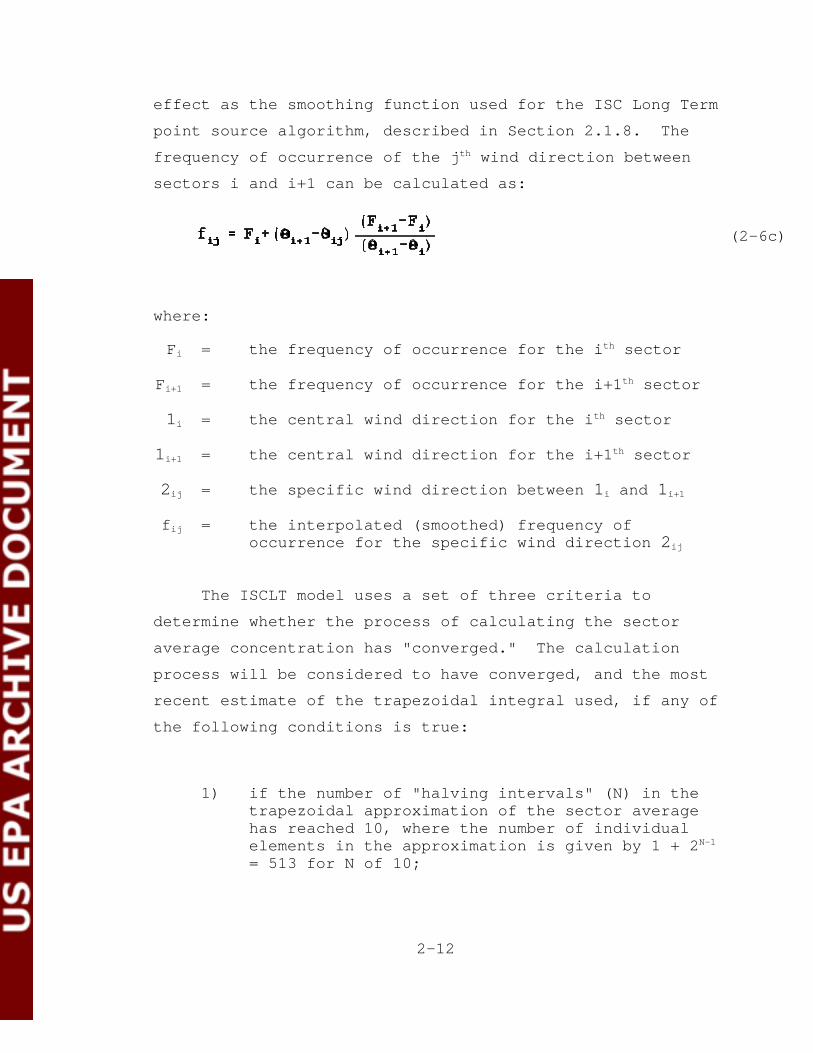
2-12

(2-6c)

effect as the smoothing function used for the ISC Long Term

point source algorithm, described in Section 2.1.8. The

frequency of occurrence of the jth wind direction between

sectors i and i+1 can be calculated as:

where:

Fi = the frequency of occurrence for the ith sector

Fi+1 = the frequency of occurrence for the i+1th sector

1i = the central wind direction for the ith sector

1i+1 = the central wind direction for the i+1th sector

2ij = the specific wind direction between 1i and 1i+1

fij = the interpolated (smoothed) frequency ofoccurrence for the specific wind direction 2ij

The ISCLT model uses a set of three criteria to

determine whether the process of calculating the sector

average concentration has "converged." The calculation

process will be considered to have converged, and the most

recent estimate of the trapezoidal integral used, if any of

the following conditions is true:

1) if the number of "halving intervals" (N) in thetrapezoidal approximation of the sector averagehas reached 10, where the number of individualelements in the approximation is given by 1 + 2N-1

= 513 for N of 10;

2-13

2) if the estimate of the sector average hasconverged to within a tolerance of 0.02 (i.e., 2percent), for two successive iterations, and atleast 2 halving intervals have been completed (aminimum of 5 wind direction simulations); or

3) if the estimate of the sector averageconcentration is less than 1.0E-10, and at least2 halving intervals have been completed.

The first condition essentially puts a time limit on the

integration process, the second condition checks for the

accuracy of the estimate of the sector average, and the

third condition places a lower threshold limit that avoids

convergence problems associated with very small

concentrations where truncation error may be significant.

2-14

2.2.4 The Long-Term Open Pit Source Model

The ISC Long Term Open Pit Source Model is based on

the use of the long term area source model described in

Section 2.2.3. The escape fractions and adjusted mass

distribution for particle emissions from an open pit, and

the determination of the size, shape and location of the

effective area source used to model open pit emissions are

described in Section 1.2.4. For the Long Term model, a

sector average value for open pit sources is calculated by

determining an effective area for a range of wind

directions within the sector and increasing the number of

wind directions used until the result converges, as

described in Section 2.2.3 for the Long Term area source

model. The contribution from each effective area used

within a sector is calculated using the Short Term area

source model described in Section 1.2.3.

2.3 THE ISC LONG-TERM DRY DEPOSITION MODEL

2.3.1 General

The concepts upon which the ISC long-term dry

deposition model are based are discussed in Sections

1.1.6.3 and 1.3.

2-15

(2-7)

2.3.2 Point and Volume Source Emissions

The seasonal deposition at the point located at a

particular distance (r) and direction (2) with respect to

the base of a stack or the center of a volume source for

particulates in the nth particle size category is given by:

where the vertical term for deposition, Vdn, was defined in

Section 1.3.2. K and D are described in Equations (1-1)

and (1-63), respectively. QJ is the product of the total

time during the lth season, of the seasonal emission rate Q

for the ith wind-speed category, kth stability category.

For example, if the emission rate is in grams per second

and there are 92 days in the summer season (June, July, and

August), QJ,l-3 is given by 7.95 x 106 Ql-3. It should be

noted that the user need not vary the emission rate by

season or by wind speed and stability. If an annual

average emission rate is assumed, QJ is equal to 3.15 x 107

Q for a 365-day year. For a plume comprised of N particle

size categories, the total seasonal deposition is obtained

by summing Equation (2-7) over the N particle size

categories. The program also sums the seasonal deposition

values to obtain the annual deposition.

2-16

2.3.3 Area and Open Pit Source Emissions

The area and open pit source dry deposition

calculations for the ISCLT model are based on the numerical

integration algorithm for modeling area sources used by the

ISCST model. Section 1.3.4, Equation (1-88), describes the

numerical integration for the Short Term model that is

applied to specific wind directions by the Long Term model

in a trapezoidal integration to calculate the sector

average. The process of calculating sector averages for

area sources in the Long Term model is described by

Equation (2-6) in Section 2.2.3.

3-1

3.0 REFERENCES

Bowers, J.F., J.R. Bjorklund and C.S. Cheney, 1979: Industrial Source Complex (ISC) Dispersion ModelUser's Guide. Volume I, EPA-450/4-79-030, U.S.Environmental Protection Agency, Research TrianglePark, North Carolina 27711.

Bowers, J.R., J.R. Bjorklund and C.S. Cheney, 1979: Industrial Source Complex (ISC) Dispersion ModelUser's Guide. Volume II, EPA-450/4-79-031, U.S.Environmental Protection Agency, Research TrianglePark, North Carolina 27711.

Briggs, G.A., 1969, Plume Rise, USAEC Critical ReviewSeries, TID-25075, National Technical InformationService, Springfield, Virginia 22161.

Briggs, G.A., 1979: Some Recent Analyses of Plume RiseObservations, In Proceedings of the SecondInternational Clean Air Congress, Academic Press, NewYork.

Briggs, G.A., 1972: Discussion on Chimney Plumes inNeutral and Stable Surroundings. Atmos. Environ., 6,507-510.

Briggs, G.A., 1974: Diffusion Estimation for SmallEmissions. In ERL, ARL USAEC Report ATDL-106. U.S.Atomic Energy Commission, Oak Ridge, Tennessee.

Briggs, G.A., 1975: Plume Rise Predications. In Lectureson Air Pollution and Environmental Impact Analysis,American Meteorological Society, Boston,Massachusetts.

Byun, D.W. and R. Dennis, 1995: Design Artifacts inEulerian Air Quality Models: Evaluation of theEffects of Layer Thickness and Vertical ProfileCorrection on Surface Ozone Concentrations. Atmos.Environ., 29, 105-126.

3-2

Chico, T. and J.A. Catalano, 1986: Addendum to the User'sGuide for MPTER. Contract No. EPA 68-02-4106, U.S.Environmental Protection Agency, Research TrianglePark, North Carolina 27711.

Cramer, H.E., et al., 1972: Development of Dosage Modelsand Concepts. Final Report Under ContractDAAD09-67-C-0020(R) with the U.S. Army, Desert TestCenter Report DTC-TR-609, Fort Douglas, Utah.

Dumbauld, R.K. and J.R. Bjorklund, 1975: NASA/MSFCMultilayer Diffusion Models and Computer Programs --Version 5. NASA Contractor Report No. NASA CR-2631,National Aeronautics and Space Administration, GeorgeC. Marshall Space Center, Alabama.

Dyer, A.J., 1974: A review of flux-profile relationships. Boundary-Layer Meteorol., 7, 363-372.

Environmental Protection Agency, 1985: Guideline forDetermination of Good Engineering Practice StackHeight (Technical Support Document for the StackHeight Regulations) - Revised, EPA-450/4-80-023R, U.S.Environmental Protection Agency, Research TrianglePark, NC 27711. (NTIS No. PB 85-225241)

Environmental Protection Agency, 1992. Comparison of aRevised Area Source Algorithm for the IndustrialSource Complex Short Term Model and Wind Tunnel Data. EPA Publication No. EPA-454/R-92-014. U.S.Environmental Protection Agency, Research TrianglePark, NC. (NTIS No. PB 93-226751)

Environmental Protection Agency, 1992. SensitivityAnalysis of a Revised Area Source Algorithm for theIndustrial Source Complex Short Term Model. EPAPublication No. EPA-454/R-92-015. U.S. EnvironmentalProtection Agency, Research Triangle Park, NC. (NTISNo. PB 93-226769)

Environmental Protection Agency, 1992. Development andEvaluation of a Revised Area Source Algorithm for theIndustrial Source Complex Long Term Model. EPA

3-3

Publication No. EPA-454/R-92-016. U.S. Environ-mentalProtection Agency, Research Triangle Park, NC. (NTISNo. PB 93-226777)

Environmental Protection Agency, 1994. Development andTesting of a Dry Deposition Algorithm (Revised). EPAPublication No. EPA-454/R-94-015. U.S. EnvironmentalProtection Agency, Research Triangle Park, NC. (NTISNo. PB 94-183100)

Gifford, F.A., Jr. 1976: Turbulent Diffusion - TypingSchemes: A Review. Nucl. Saf., 17, 68-86.

Hicks, B.B., 1982: Critical assessment document on aciddeposition. ATDL Contrib. File No. 81/24, Atmos.Turb. and Diff. Laboratory, Oak Ridge, TN.

Holzworth, G.C., 1972: Mixing Heights, Wind Speeds andPotential for Urban Air Pollution Throughout theContiguous United States. Publication No. AP-101,U.S. Environmental Protection Agency, ResearchTriangle Park, North Carolina 27711.

Horst, T.W., 1983: A correction to the Gaussian source-depletion model. In Precipitation Scavenging, DryDeposition and Resuspension, H.R. Pruppacher, R.G.Semonin, W.G.N. Slinn, eds., Elsevier, NY.

Huber, A.H. and W.H. Snyder, 1976: Building Wake Effectson Short Stack Effluents. Preprint Volume for theThird Symposium on Atmospheric Diffusion and AirQuality, American Meteorological Society, Boston,Massachusetts.

Huber, A.H. and W.H. Snyder, 1982. Wind tunnelinvestigation of the effects of a rectangular-shapedbuilding on dispersion of effluents from shortadjacent stacks. Atmos. Environ., 176, 2837-2848.

Huber, A.H., 1977: Incorporating Building/Terrain WakeEffects on Stack Effluents. Preprint Volume for theJoint Conference on Applications of Air Pollution

3-4

Meteorology, American Meteorological Society, Boston,Massachusetts.

Jindal, M. and D. Heinold, 1991: Development ofparticulate scavenging coefficients to model wetdeposition from industrial combustion sources. Paper91-59.7, 84th Annual Meeting - Exhibition of AWMA,Vancouver, BC, June 16-21, 1991.

McDonald, J.E., 1960: An Aid to Computation of TerminalFall Velocities of Spheres. J. Met., 17, 463.

McElroy, J.L. and F. Pooler, 1968: The St. LouisDispersion Study. U.S. Public Health Service,National Air Pollution Control Administration, ReportAP-53.

National Climatic Center, 1970: Card Deck 144 WBAN HourlySurface Observations Reference Manual 1970, Availablefrom the National Climatic Data Center, Asheville,North Carolina 28801.

Pasquill, F., 1976: Atmospheric Dispersion Parameters inGaussian Plume Modeling. Part II. PossibleRequirements for Change in the Turner Workbook Values.EPA-600/4-76-030b, U.S. Environmental ProtectionAgency, Research Triangle Park, North Carolina 27711.

Perry, S.G., R.S. Thompson, and W.B. Petersen, 1994: Considerations for Modeling Small-Particulate Impactsfrom Surface Coal Mining Operations Based on Wind-Tunnel Simulations. Proceedings Eighth JointConference on Applications of Air PollutionMeteorology, January 23-28, Nashville, TN.

Petersen, W.B. and E.D. Rumsey, 1987: User's Guide for PAL2.0 - A Gaussian-Plume Algorithm for Point, Area, andLine Sources, EPA/600/8-87/009, U.S. EnvironmentalProtection Agency, Research Triangle Park, NorthCarolina.

Pleim, J., A. Venkatram and R. Yamartino, 1984: ADOM/TADAPmodel development program. Volume 4. The dry

3-5

deposition module. Ontario Ministry of theEnvironment, Rexdale, Ontario.

Press, W., B. Flannery, S. Teukolsky, and W. Vetterling,1986: Numerical Recipes, Cambridge University Press,New York, 797 pp.

Schulman, L.L. and S.R. Hanna, 1986: Evaluation ofDownwash Modifications to the Industrial SourceComplex Model. J. Air Poll. Control Assoc., 36 (3),258-264.

Schulman, L.L. and J.S. Scire, 1980: Buoyant Line andPoint Source (BLP) Dispersion Model User's Guide. Document P-7304B, Environmental Research andTechnology, Inc., Concord, MA.

Scire, J.S. and L.L. Schulman, 1980: Modeling Plume Risefrom Low-Level Buoyant Line and Point Sources. Proceedings Second Joint Conference on Applicationsof Air Pollution Meteorology, 24-28 March, NewOrleans, LA. 133-139.

Scire, J.S., D.G. Strimaitis and R.J. Yamartino, 1990: Model formulation and user's guide for the CALPUFFdispersion model. Sigma Research Corp., Concord, MA.

Slinn, W.G.N., 1982: Predictions for particle depositionto vegetative canopies. Atmos. Environ., 16, 1785-1794.

Slinn, S.A. and W.G.N. Slinn, 1980: Predictions forparticle deposition and natural waters. Atmos.Environ., 14, 1013-1016.

Thompson, R.S., 1994: Residence Time of ContaminantsReleased in Surface Coal Mines -- A Wind Tunnel Study. Proceedings Eighth Joint Conference on Applications ofAir Pollution Meteorology, January 23-28, Nashville,TN.

3-6

Touma, J.S., J.S. Irwin, J.A. Tikvart, and C.T. Coulter,1995. A Review of Procedures for Updating Air QualityModeling Techniques for Regulatory Modeling Programs. J. App. Meteor., 34, 731-737.

Turner, D.B., 1970: Workbook of Atmospheric DispersionEstimates. PHS Publication No. 999-AP-26. U.S.Department of Health, Education and Welfare, NationalAir Pollution Control Administration, Cincinnati,Ohio.

Venkatram, A., 1988: A Simple Model for Dry Deposition andParticle Settling. Subcontractor Progress Report 2(including addendum), EPA Contract No. 68D70002, WorkAssignment No. 1-001.

Yamartino, R.J., J.S. Scire, S.R. Hanna, G.R. Carmichaeland Y.S. Chang, 1992: The CALGRID mesoscalephotochemical grid model. Volume I. Modelformulation. Atmos. Environ., 26A, 1493-1512.

INDEX-1

INDEX

Area source

deposition algorithm . . . . . . . . . . . 1-60, 2-14for the Long Term model . . . . . . . . . . 2-8, 2-9

for the Short Term model . . . . . . . . . 1-40, 1-44

Atmospheric resistance . . . . . . . . . . . . . . . 1-56Attenuation correction factor

in complex terrain . . . . . . . . . . . . . . . 1-69

Briggs plume rise formulas

buoyant plume rise . . . . . . . . . . . . . 1-7, 1-9momentum plume rise . . . . . . . . . . . . 1-8, 1-10

stack tip downwash . . . . . . . . . . . . . . . . 1-6

Building downwash procedures . . . . . . . . . . 1-24, 2-5and buoyancy-induced dispersion . . . . . . . . 1-31

effects on dispersion parameters . . . . . . . . 1-21

for the Long Term model . . . . . 1-64, 2-2, 2-4, 2-5general . . . . . . . . . . . . . . . . . . 1-5, 1-22

Huber and Snyder . . . . . . . . . . . . . . . . 1-23

Schulman and Scire . . . . . . . 1-5, 1-12, 1-28, 1-29

Schulman-Scire plume rise . . . . . . . . 1-12, 1-14virtual distances . . . . . . . . . . . . . . . 1-20

wake plume height . . . . . . . . . . . . . . . 1-12

Buoyancy flux . . . . . . . . . . . . . . . . . . 1-6, 1-14Buoyancy-induced dispersion . . . . . . . . 1-30, 1-31, 2-6

Buoyant plume rise

stable . . . . . . . . . . . . . . . . . . . . . . 1-9unstable and neutral . . . . . . . . . . . . . . . 1-7

Cartesian receptor network . . . . . . . . . . . . . . 1-3

Complex terrain modeling

Short Term model . . . . . . . . . . . . . 1-63, 1-72Crossover temperature difference . . . . . . . . . . . 1-7

Crosswind distance . . . . 1-2, 1-3, 1-4, 1-64, 1-65, 2-4

Decay coefficient . . . . . . . . . . . . . . . . . . 1-40Decay term . . . . . . . . . . . . . . . . 1-3, 1-39, 1-65

for the Long Term model . . . . . . . 1-65, 2-3, 2-7

for the Short Term model . . . . . . . . . 1-39, 1-69

INDEX-2

Depletionfor the dry deposition algorithm . . . . . . . . 1-39

for the wet deposition algorithm . . . . . . . . 1-61

Deposition velocity . . . . . . . . . . . . . . 1-35, 1-54Direction-specific building dimensions . . . . 1-22, 1-29

with Huber-Snyder downwash . . . . . . . . . . . 1-29

Dispersion coefficientssee Dispersion parameters . . . . . . . . 1-15, 1-66

Dispersion parameters

for the Long Term model . . . . . . . . . . . . . 2-4

McElroy-Pooler . . . . . . . . . . . . . . 1-15, 1-19Pasquill-Gifford . . . . . . . 1-15, 1-16, 1-17, 1-18

Distance-dependent plume rise . . . . . . . . . . . . 1-13

Downwind distance . . . . . 1-2, 1-3, 1-4, 1-64, 1-65, 2-4and virtual distance . . . . . . . . . . . . . . 1-20

for area sources . . . . . . . . . . . . . . . . 1-44

for building wake dispersion . . . . . . . . . . 1-24for dispersion coefficients . . . . . . . . . . 1-15

Dry deposition . . . . . . . . . . . . . . 1-3, 1-65, 2-12

for the Long Term model . . . . . . . . . . . . 2-12

for the Short Term model . . . . . . . . . . . . 1-53Elevated terrain . . . . . . . . . . . . . 1-34, 1-67, 2-7

truncation above stack height . . . . . . . . . 1-34

Entrainment coefficient . . . . . . . . . . . . . . . 1-14Final plume rise . . . . . . . . . . . . . . . . . . 1-30

distance to . . . . . . . . . . . . . . . . . . . 1-7

stable . . . . . . . . . . . . . . . . . . . 1-9, 1-10unstable or neutral . . . . . . . . . . . . 1-7, 1-8

Flagpole receptor . . . . . . . . . . . . . . . . . . 1-32

Gaussian plume model . . . . . . . . . . . . . . 1-2, 1-63

sector averages for complex terrain . . . . . . 1-63sector averages for Long Term . . . . . . . . . . 2-1

GEP stack height . . . . . . . . . . . . . . . 1-12, 1-30

Gradual plume rise . . . . . . . . . . . . . . . . . 1-10for buoyant plumes . . . . . . . . . . . . . . . 1-10

for Schulman-Scire downwash . . . . . . . 1-13, 1-14

stable momentum . . . . . . . . . . . . . . . . 1-11

INDEX-3

unstable and neutral momentum . . . . . . . . . 1-11used for wake plume height . . . . . . . . . . . 1-12

Half life . . . . . . . . . . . . . . . . . . . . . . 1-40

Huber-Snyder downwash algorithm . . . . . . . . . . . . 1-5Initial lateral dimension

for the Long Term model . . . . . . . . . . . . . 2-5

for volume sources . . . . . . . . . . . . 1-42, 1-43Initial plume length

Schulman-Scire downwash . . . . . . . . . . . . 1-13

Initial plume radius

Schulman-Scire downwash . . . . . . . . . . . . 1-13Initial vertical dimension

for volume sources . . . . . . . . . . . . . . . 1-43

Intermediate terrain . . . . . . . . . . . . . . . . 1-72Jet entrainment coefficient . . . . . . . . . . 1-11, 1-14

Lateral dispersion parameters . . . . . . 1-16, 1-19, 1-30

for the Long Term model . . . . . . . . . . . . . 2-4Lateral virtual distance

for the Long Term model . . . . . . . 1-64, 2-3, 2-4

Lateral virtual distances

for building downwash . . . . . . . . . . . . . 1-26Line source

approximation for Schulman-Scire sources . . . . 1-13

Line sources, modeled as volumes . . 1-40, 1-42, 1-43, 2-8Linear decay factor

Schulman-Scire downwash . . . . . . . . . 1-13, 1-29

Long-term dispersion model . . . . . . . . . . . . . . 2-1McElroy-Pooler dispersion parameters

see Dispersion parameters . . . . . . . . . . . 1-19

Mixing heights . . . . . . . . . . . . . . . . . . . 1-33

Momentum flux . . . . . . . . . . . . . . . . . . 1-6, 1-14Momentum plume rise . . . . . . . . . . . 1-11, 1-23, 1-29

stable . . . . . . . . . . . . . . . . . . . . . 1-10

unstable and neutral . . . . . . . . . . . . . . . 1-8Open pit source

deposition algorithm . . . . . . . . . . . 1-60, 2-14

for the Long Term model . . . . . . . . . . . . 2-12

INDEX-4

for the Short Term model . . . . . . . . . . . . 1-48Open pit sources . . . . . . . . . . . . . . . 1-41, 1-48

Pasquill-Gifford dispersion parameters

see Dispersion parameters . . . . . . . . . . . 1-16Plume rise

for Schulman-Scire downwash . . . . . . . . . . 1-12

for the Long Term model . . . . . . . . . . . . . 2-4for the Short Term model . . . . . . . . . . 1-5, 1-65

Point source

deposition algorithm . . . . . . . . . . . 1-59, 2-13

dispersion parameters . . . . . . . . . . . 1-15, 2-4for the Long Term model . . . . . . . . . . . . . 2-1

for the Short Term model . . . . . . . . . . . . . 1-2

Polar receptor network . . . . . . . . . . . . . . . . 1-3Receptors

calculation of source-receptor distances . . 1-3, 1-4

Ruraldispersion parameters . . . . . . . . . . . . . 1-15

virtual distances . . . . . . . . . . . . 1-20, 1-25

Schulman-Scire downwash algorithm . . . . . . . . . . . 1-5

Short-term dispersion model . . . . . . . . . . . . . . 1-1Sigma-y . . . . . . . . . . . . . . . . . . . . 1-15, 1-66

Sigma-z . . . . . . . . . . . . . . . . . . . . 1-15, 1-66

Smoothing functionfor the Long Term model . . . . . . . . . . 2-3, 2-7

Stability parameter . . . . . . . . . . . . . . . 1-9, 1-14

Stack-tip downwash . . . . . . . . . . . . . . . . . . 1-6for wake plume height . . . . . . . . . . . . . 1-12

Uniform vertical mixing . . . . . . . . . . . . . . . 1-32

Urban

decay term for SO2 . . . . . . . . . . . . . . . 1-40dispersion parameters . . . . . . . . . . . . . 1-15

virtual distances . . . . . . . . . . . . 1-20, 1-26

Vertical dispersion parameters . . . . . 1-17, 1-18, 1-19Vertical term . . . . . . . . . . . . 1-3, 1-45, 1-65, 2-6

for gases and small particulates . . . . . . . . 1-31

for large particulates . . . . . . . . . . . . . . 2-7

INDEX-5

for the Long Term model . . . . . . . 1-65, 2-3, 2-6for the Short Term model . . . . . . . . . 1-31, 1-67

for uniform vertical mixing . . . . . . . 1-32, 1-33

in complex terrain . . . . . . . . . . . . . . . 1-67in elevated terrain . . . . . . . . . . . . 1-34, 2-7

Vertical virtual distances

for building downwash . . . . . . . . . . 1-25, 1-26Virtual distances . . . 1-20, 1-21, 1-28, 1-29, 1-41, 1-45

for the Long Term model . . . . . . . . . . 2-4, 2-5

for volume sources . . . . . . . . . . . . . . . 1-41

Virtual point source . . . . . . 1-41, 1-64, 2-2, 2-8, 2-9Volume source . . . . . . . . . . . . . . . . . . . . 1-43

deposition algorithm . . . . . . . . . . . 1-59, 2-13

for the Long Term model . . . . . . . . . . . . . 2-8for the Short Term model . . . . . . . . . 1-40, 1-41

Wet deposition

for the Short Term model . . . . . . . . . . . . 1-61Wind speed

minimum wind speed for modeling . . . . . . . . . 1-5

Wind speed profile . . . . . . . . . . . . 1-4, 1-65, 2-4