volume 4, number 1, pages 16{38 - ualberta.ca · international journal of °c 2007 institute for...
TRANSCRIPT
INTERNATIONAL JOURNAL OF c© 2007 Institute for ScientificNUMERICAL ANALYSIS AND MODELING Computing and InformationVolume 4, Number 1, Pages 16–38
CONVERGENCE AND SUPERCONVERGENCE OF ANONCONFORMING FINITE ELEMENT ON ANISOTROPIC
MESHES
SHIPENG MAO, SHAOCHUN CHEN, AND DONGYANG SHI
(Communicated by Zhimin Zhang)
Abstract. The main aim of this paper is to study the error estimates of a
nonconforming finite element for general second order problems, in particular,
the superconvergence properties under anisotropic meshes. Some extrapolation
results on rectangular meshes are also discussed. Finally, numerical results are
presented, which coincides with our theoretical analysis perfectly.
Key Words. nonconforming finite element, anisotropic meshes, superconver-
gence, extrapolation.
1. Introduction
It is well-known that regular assumption or quasi-uniform assumption [10, 13] offinite element meshes is a basic condition in the analysis of finite element approxima-tion both for conventional conforming and nonconforming elements. However, withthe advances of the finite element methods and its applications to other fields andmore complex problems, the above regular or quasi-uniform assumption becomesquite a restriction in practice for some problems in the finite element methods. Forexample, the solution may have anisotropic behavior in part of the domain, thatis to say, the solution varies significantly only in certain directions. Such prob-lems are frequently encountered in perturbed convection-diffusion-reaction equa-tions where boundary or interior layers appear. In such cases, it is more effective touse anisotropic meshes with a small mesh size in the direction of the rapid variationof the solution and a larger mesh size in the perpendicular direction. Consider abounded convex domain Ω ⊂ R2. Let Jh be a family of meshes of Ω. Denote thediameter of an element K and the diameter of the inscribed circle of K by hK andρK , respectively. h = max
K∈Jh
hK . It is assumed in the classical finite element theory
that hK
ρK≤ C, where C be a positive constant independent of K and the function
considered. Such assumption is no longer valid in the case of anisotropic meshes.Conversely, anisotropic elements are characterized by hK
ρK→ ∞ as h → 0. Some
early papers have been written to prove error estimates under more general condi-tions (refer to [7, 25]). Recently, much attention is paid to FEMs with anisotropicmeshes. In particular, for anisotropic rectangular meshes we refer to Acosta [1, 2],Apel [3, 4, 5, 6], Chen [16, 17, 31, 38], Duran [22, 23], Shenk [37] and referencestherein, and for narrow quadrilateral meshes to Zenisek [45]. But to our best knowl-edge, there are few papers focused on the nonconforming elements under anisotropicmeshes.
On the other hand, researchers have observed that for certain classes of problemsthe rate of convergence of the finite element solution and/or its derivatives at some
Received by the editors July 1, 2004 and, in revised form, June 18, 2005.2000 Mathematics Subject Classification. 65N30, 65N15.This research is supported by NSF of China (No.10471133, 10590353, 10371113).
16
SUPERCONVERGENCE OF NONCONFORMING FE ON ANISOTROPIC MESHES 17
special points exceeds the best global rate. This phenomenon has been termed ”superconvergence” and has been analyzed mathematically because of its practicalimportance in engineering computations. Also some postprocessing methods havebeen developed to improve the accuracy of finite element solution. Many super-convergence results about conforming FEMs have been obtained, see e.g., [14, 26,29, 43]. Do the superconvergence results of conforming elements still hold for thosenonconforming ones? The answer is affirmative. In [15, 39], the superconvergence ofWilson element is studied and the superconvergence estimate of the gradient erroron the centers of elements is obtained. Recently, some superconvergentce resultsof rotated Q1 type elements are derived for quasi-uniform meshes in [30, 32]. Onthe other hand, Wang [44] proposed a least-square surface fitting method to obtainthe superconvergence under quasi-uniform mesh assumption. The main feature oftheir method is to apply an L2 projection on a coarser mesh with size τ =O(hα)(α ∈ (0, 1)). At the same time, extrapolation is widely used in the finite elementmethod. Interested readers are referred to [8, 9, 29, 35, 36] for extrapolation resultsof the conforming linear and bilinear element.
In this work, we first study the anisotropic interpolation error on anisotropicaffine quadrilateral meshes of a five-node nonconforming finite element proposedby [24, 30], and the optimal consistency error is derived by a detailed analysis foranisotropic affine quadrilaterals, which extends the results of [38] for the rectan-gular meshes. We comment that since the interpolation of the original rotated Q1
element does not satisfy the anisotropic interpolation properties, reference [4] dealswith the modified anisotropic rectangular rotated Q1 element with the shape spacespan1, ξ, η, ξ2. There has been other works for the modified rotated Q1 element(cf. [5, 19, 28]).
In section §3, following the technique developed in [30, 38], we obtain a higherorder O(h2) of consistency error under anisotropic rectangular meshes. Based onthis fact and some other higher order error estimates proved in this section, asuperconvergent approximation between the interpolation of the exact solution andthe finite element solution is derived. Then a superconvergent estimate on thecenters of elements is obtained, and the global superconvergence O(h2) for thegradient of the solution is also derived with the aid of a suitable postprocessingmethod.
In section §4, for regular rectangular meshes, we study some error expansionsfor the five-node nonconforming element. Based on these expansions, we obtain asharp error estimates O(h3) by extrapolations. In the last section, some numericalexamples are presented to validate our theoretical analysis.
Finally, we recall some notations and terminology (or refer to [10, 13]). Let (·, ·)denote the usual L2 -inner product and ‖u‖r,p,Ω (resp. |u|r,p,Ω) be the usual norm(resp. semi-norm) for the Sobolev space W r,p(Ω). When p = 2, denote W 2,r(Ω)by Hr(Ω). Throughout this paper, C will be used as a generic positive constant,which is independent of hK , and may be independent of the aspect ratio hK
ρKin §2
and §3.
2. Error estimates for general second order problems under anisotropicaffine quadrilaterals
Let K = [−1, 1] × [−1, 1] be the reference element. Its four vertices are: a1 =(−1,−1), a2 = (1,−1), a3 = (1, 1), a4 = (−1, 1), and its four sides are l1 = a1a2, l2 =a2a3, l3 = a3a4, l4 = a4a1.
The nonconforming five-node element[24,30] (K, P , Σ) on K is defined as follows:
(2.1) Σ = v1, v2, v3, v4, v5, P = span1, ξ, η, ϕ(ξ), ϕ(η),
18 S. P. MAO, S. CHEN, AND D. SHI
where vi = 1
|li|∫
livds, i = 1, 2, 3, 4. v5 = 1
|K|∫
Kvdξdη, ϕ(t) = 1
2 (3t2 − 1).It can be easily checked that the interpolation defined above is properly posed,
the interpolation function is as follows:
(2.2) Πv = v5+12(v2−v4)ξ+
12(v3−v1)η+
12(v2+v4−2v5)ϕ(ξ)+
12(v3+v1−2v5)ϕ(η).
The following lemma shows that the interpolation Π defined as (2.2) possessesthe anisotropic properties[6,16].
Lemma 2.1. The interpolation operator Π has the anisotropic interpolation prop-erties, i.e., for |α| = 1,
(2.3) ‖Dα(v − Πv)‖0,K ≤ C|Dαv|1,K .
Proof. When α = (1, 0),
(2.4) DαΠv =∂Πv
∂ξ=
12(v2 − v4) +
12(v2 + v4 − 2v5)ϕ
′(ξ)
Noticed that r = dimDαP = 2. Obviously, 1, ϕ′(ξ) is a basis of DαP . Let
DαΠv = β1 + β2ϕ′(ξ),
where
β1 =12(v2 − v4) =
14(∫
l2
v(1, η)dη −∫
l4
v(−1, η)dη) =1
|K|
∫
K
∂v
∂ξdξdη,
β2 =12(v2 + v4 − 2v5) =
14(∫
l2
v(1, η)dη +∫
l4
v(−1, η)dη −∫
K
v(ξ, η)dξdη)
=1
|K|
∫
K
ξ∂v
∂ξdξdη.
For any w ∈ H1(K), define
(2.5) F1(w) =1
|K|
∫
K
wdξdη, F2(w) =1
|K|
∫
K
ξwdξdη.
Apparently, Fj ∈ (H1(K))′, j = 1, 2. Employing the basic anisotropic interpolation
theorem[16] yields‖Dα(v − Πv)‖0,K ≤ C|Dαv|1,K .
Similarly, we can prove that (2.3) is valid for α = (0, 1). This completes theproof.
Given a general affine quadrilateral K with four vertices ai and sides li =aiai+1, i = 1, 2, 3, 4, a5 = a1, let hK1 denote the length of the longest edge ofK and hK2 = |K|/hK1 is the corresponding height. Then the affine mappingFK : K −→ K can be written as
(2.6)
x = b1 + b1,1ξ + b1,2η,
y = b2 + b2,1ξ + b2,2η
For simplicity, we assume Ω ⊂ R2 to be a convex polygon composed by a family ofaffine quadrilaterals meshes Jh which needs not satisfy the regular and inverse as-sumption conditions, but satisfies the maximal angle condition[6]. Furthermore, theaxes can be rotated such that the elements satisfy the coordinate system condition[6].The definition of the maximal angle condition and coordinate system condition arelisted as follows.
Maximal angle condition: There is a constant σ∗ < π (independent of h and K)
SUPERCONVERGENCE OF NONCONFORMING FE ON ANISOTROPIC MESHES 19
such that the maximal interior angle σ of any element K is bounded by σ∗, i.e.,σ < σ∗.
Coordinate system condition: The angle ϑ between the longer sides and the x-axisis bounded by | sin ϑ| ≤ hK2
hK1.
Based on reference [6], we have the following results.
Lemma 2.2[6]. Assume that an affine quadrilateral element K satisfies the max-imal angle condition and the coordinate system condition. Then the entries of thematrix B = (bi,j)2i,j=1 ∈ R2×2 and of its inverse B−1 = (b−1
i,j )2i,j=1 ∈ R2×2 satisfythe following conditions:
(2.7) |bi,j | ≤ minhKi, hKj, i, j = 1, 2,
(2.8) |b−1i,j | ≤ minh−1
Ki, h−1Kj, i, j = 1, 2.
Lemma 2.3[6]. Let α be a multiple-index, then
(2.9)∑
|α|=m
|Dαv| ≤ C∑
|s|=m
hsK |Dsv|, |Dαv| ≤ Chα
K
∑
|s|=|α||Dsv|,
(2.10)∑
|α|=m
|Dαv| ≤ C∑
|s|=m
h−sK |Dsv|,
where hsK = hs1
K1hs2K2, s = (s1, s2), and hK is used as diameter of element K in §1.
Define the finite element space as
Vh = vh|vh = vh|K FK ∈ P ,
∫
F
[vh]ds = 0, F ⊂ ∂K,∀K ∈ Jh,
where we denote sides of elements by F and by [v] the jump of the function v onthe sides F . For boundary sides we identify [v] with v.
Let the general element K be a quadrilateral in x − y plane, the interpolateoperator is defined as
ΠK : H2(K) → P F−1K ,ΠKv = (Πv) F−1
K , Πh : H2(Ω) → Vh, Πh|K = ΠK .
We consider the following general second-order elliptic boundary value problem
(2.11)
Lu = −
2∑
i,j=1
∂j(αij∂iu) +2∑
i=1
αi∂iu + γu = f, in Ω
u = 0, on ∂Ω.
where ∂iu = ∂u∂xi
, (x1, x2) = (x, y), the coefficients αij , αi ∈ W 1,∞(Ω), 1 ≤ i, j ≤ 2and γ ≥ 0, the right hand term f ∈ L2(Ω).
We assume that the differential operator L is uniformly elliptic, i.e., there existsa positive constant C such that
C−1(ξ21 + ξ2
2) ≤2∑
i,j=1
αijξiξj ≤ C(ξ21 + ξ2
2)
for all points (x, y) ∈ Ω and real vectors (ξ1, ξ2) ∈ R2.Let V = H1
0 (Ω), then the weak form of (2.11) is:
(2.12)
Find u ∈ V, such that
a(u, v) = f(v), ∀ v ∈ V

20 S. P. MAO, S. CHEN, AND D. SHI
where
a(u, v) =∫
Ω
2∑
i,j=1
αij∂iu∂jv +2∑
i=1
αi∂iuv + γuv
dxdy,
f(v) =∫
Ω
fvdxdy.
The approximation of (2.12) reads as follows:
(2.13)
Find uh ∈ Vh, such that
ah(uh, vh) = f(vh), ∀ vh ∈ Vh
with
ah(uh, vh) =∑
K∈Jh
∫
K
2∑
i,j=1
αij∂iuh∂jvh +2∑
i=1
αi∂iuhvh + γuhvh
dxdy.
Set
(2.14) ‖ · ‖h =
( ∑
K∈Jh
| · |21,K
) 12
.
Then it is easy to see that ‖ · ‖h is the norm over Vh .
The following theorem is the main results of this section.
Theorem 2.1. Let Jh be a partition of Ω by affine quadrilaterals which satis-fies the maximal angle condition, but may not satisfy the regular conditions. Let uand uh be the solution of problem (2.11) and (2.13) respectively. Then there hold
(2.15) ‖u− uh‖h ≤ Ch(|u|2,Ω + |u|1,Ω)
and
(2.16) ‖u− uh‖0,Ω ≤ Ch2(|u|2,Ω + |u|1,Ω).
Proof. The second Strang’s lemma[10,13] reads as
(2.17) ‖u− uh‖h ≤ C
(inf
vh∈Vh
‖u− vh‖h + supvh∈Vh
|ah(u, vh)− (f, vh)|‖vh‖h
).
Now we consider the first term on the right hand of (2.17), i.e., the interpolationerror.
SUPERCONVERGENCE OF NONCONFORMING FE ON ANISOTROPIC MESHES 21
By using of (2.3), (2.9) and (2.10), the approximation error an be estimated as
(2.18)
infvh∈Vh
‖u− vh‖h ≤ ‖u−Πhu‖h
=
( ∑
K∈Jh
|u−ΠKu|21,K
) 12
=
∑
K∈Jh
∑
|α|=1
‖Dα(u−ΠKu)‖20,K
12
=
∑
K∈Jh
∑
|α|=1
h−2αK (hK1hK2)‖Dα(u− Πu)‖2
0,K
12
≤ C
∑
K∈Jh
∑
|α|=1
h−2αK (hK1hK2)|Dαu|2
1,K
12
=C
∑
K∈Jh
∑
|α|=1
h−2αK (hK1hK2)
∑
|β|=1
‖Dα+β u‖20,K
12
≤C
∑
K∈Jh
∑
|α|=1|β|=1
h2βK ‖Dα+βu‖20,K
12
≤ C
∑
K∈Jh
∑
|β|=1
h2βK |Dβu|21,K
12
≤ Ch|u|2,Ω.
Then we turn to the second term on the right hand of (2.17), i.e., the consistencyerror. By Green’s formula, it follows from the conventional techniques of consistencyerror estimates[27,38] that,(2.19)
Eh(u, vh) = ah(u, vh)− f(vh) =∑
K∈Jh
∫
∂K
2∑
i,j=1
αij∂u
∂xinjvhds
=∑
K∈Jh
4∑m=1
∫
lm
2∑
i,j=1
(αij∂u
∂xi− P0m(αij
∂u
∂xi))(vh − P0mvh)nmjds
=∑
K∈Jh
4∑m=1
2∑
i,j=1
Amij .
where P0mv = 1|lm|
∫lm
vds, m = 1, 2, 3, 4. ni = (ni1, ni2) denotes the usual unitnormal of side li.
22 S. P. MAO, S. CHEN, AND D. SHI
We concentrate on a general element K, and for all i, j,m ,(2.20)
Amij =
∫
lm
(αij
∂u
∂xi− P0m(αij
∂u
∂xi))
(vh − P0mvh)nmjds
= |lm|nmj
∫
lm
(
αij∂u
∂xi− P0m(
αij
∂u
∂xi)
)(vh − P0mvh
)ds
≤ C|lm|nmj |
αij∂u
∂xi|1,K |vh|1,K
≤ C|lm|nmj
∑
|β|=1
‖Dβ(
αij∂u
∂xi)‖2
0,K
12
∑
|β|=1
‖Dβ vh‖20,K
12
≤ C|lm|nmj
hK1hK2
∑
|β|=1
h2βK ‖Dβ(αij
∂u
∂xi)‖20,K
12
∑
|β|=1
h2βK ‖Dβvh‖20,K
12
≤ C|lm|nmj
hK1hK2
∑
|β|=1
h2βK (| ∂u
∂xi|21,K + ‖ ∂u
∂xi‖20,K)
12
∑
|β|=1
h2βK ‖Dβvh‖20,K
12
.
If |lm|nmj ≤ ChK2, we can obtain
(2.21) Amij ≤ C
∑
|β|=1
h2βK (| ∂u
∂xi|21,K + ‖ ∂u
∂xi‖20,K)
12
|vh|1,K ,
Unfortunately, when |lm|nmj ≤ ChK1 and hK1hK2
−→ ∞ (which is the case inanisotropic meshes), we will get the following pessimistic estimate,
(2.22) Amij ≤ C
hK1
hK2
∑
|β|=1
h2βK (| ∂u
∂xi|21,K + ‖ ∂u
∂xi‖20,K)
12
|vh|1,K .
Therefore, we have to develop a different trick to derive the optimal consistencyerror estimates for anisotropic meshes. ∀i, j = 1, 2, let us consider A1
ij and A3ij
together, we expect that there holds some cancellation between the two oppositesides l1, l3 ⊂ ∂K.
Since |l1| = |l3|, n1j = −n3j , we have
(2.23)
A1ij + A3
ij
=∫
l1
(αij
∂u
∂xi− P01(αij
∂u
∂xi))
(vh − P01vh) n1jds
+∫
l3
(αij
∂u
∂xi− P03(αij
∂u
∂xi))
(vh − P03vh)n3jds
= |l1|n1j [∫ 1
−1
(
αij∂u
∂xi(ξ,−1)− P01(
αij
∂u
∂xi)
)(vh(ξ,−1)− P01vh
)dξ
−∫ 1
−1
(
αij∂u
∂xi(ξ, 1)− P03(
αij
∂u
∂xi)
) (vh(ξ, 1)− P03vh
)dξ].

SUPERCONVERGENCE OF NONCONFORMING FE ON ANISOTROPIC MESHES 23
Moreover, noticed ∂vh
∂ξ is a constant on K, then
(2.24)
vh(ξ,−1)− P01vh =12
∫ 1
−1
vh(ξ,−1)dt− 12
∫ 1
−1
vh(t,−1)dt
=12
∫ 1
−1
∫ ξ
t
∂vh
∂z(z,−1)dzdt =
12
∫ 1
−1
∫ ξ
t
∂vh
∂z(z, 1)dzdt
= vh(ξ, 1)− P03vh,
Set V = αij∂u∂xi
, then(2.25)
A1ij + A3
ij
= |l1|n1j
∫ 1
−1
(V (ξ,−1)− V (ξ, 1)− P01V + P03V
)dξ
∫ 1
−1
∫ ξ
t
∂vh
∂zdzdt
= |l1|n1j
∫ 1
−1
(−
∫ 1
−1
∂V (ξ, ζ)∂ζ
dζ +12
∫ 1
−1
∫ 1
−1
∂V (z, ζ)∂ζ
dzdζ
)dξ
∫ 1
−1
∫ ξ
t
∂vh
∂zdzdt
≤ ChK1
∥∥∥∂V
∂ζ
∥∥∥0,K
∥∥∥∂vh
∂z
∥∥∥0,K
≤ ChK1
∥∥∥∂ (αij
∂u∂xi
)∂ζ
∥∥∥0,K
∥∥∥∂vh
∂z
∥∥∥0,K
≤ C1
hK1hK2hK1h
(0,1)K
∣∣∣αij∂u
∂xi
∣∣∣1,K
hK1
∣∣∣vh
∣∣∣1,K
≤ ChK1
(| ∂u
∂xi|1,K + ‖ ∂u
∂xi‖0,K
) ∣∣∣vh
∣∣∣1,K
A combination of (2.19) and (2.25) yields
(2.26) Eh(u, vh) ≤ Ch(|u|2,Ω + |u|1,Ω)‖vh‖h.
Then (2.15) follows from (2.17), (2.18) and (2.26), and an application of A-Ntechnique[10,13] completes the proof.
3. Anisotropic superconvergence analysis
In this section, we focus on the superconvergence behavior of the element. Forthe sake of simplicity, we consider problem (2.11) with the assumption that αij =0, i 6= j. Let Ω ⊂ R2 be a convex polygon composed by a family of rectangularmeshes Jh which needs not satisfy the regular conditions. For any K ∈ Jh, denoteits barycenter by (xK , yK), the length of the edges parallel to x-axis and y-axis by2hK1, 2hK2 respectively. Then the mapping FK : K −→ K is defined as
(3.1)
x = xK + hK1ξ,
y = yK + hK2η.
Now, we prepare to derive a superclose result.
Theorem 3.1. Let Jh be a family of anisotropic rectangular meshes, and u, uh, Ihuare the same as in Theorem 2.1, u ∈ H3(Ω)∩H1
0 (Ω), αii ∈ W 2,∞(Ω), αi ∈ W 1,∞(Ω), i =1, 2, γ ∈ L∞(Ω), then there holds the following superclose property
(3.2) ‖Πhu− uh‖h ≤ Ch2(|u|3,Ω + |u|2,Ω + |u|1,Ω).
Proof. It can be proved easily that
(3.3)C‖Πhu− uh‖2h ≤ ah(Πhu− uh, Πhu− uh)
= ah(Πhu− u, Πhu− uh) + ah(u− uh, Πhu− uh).

24 S. P. MAO, S. CHEN, AND D. SHI
Set vh = Πhu− uh,w = Πhu− u. Let us consider ah(w, vh) first,(3.4)
ah(w, vh) =∑
K∈Jh
∫
K
(2∑
i=1
αii∂w
∂xi
∂vh
∂xi+
2∑
i=1
αi∂w
∂xivh + γwvh
)dxdy
=∑
K∈Jh
∫
K
(2∑
i=1
P0αii∂w
∂xi
∂vh
∂xi+
2∑
i=1
P0αi∂w
∂xivh + γwvh
)dxdy
+∑
K∈Jh
∫
K
(2∑
i=1
(αii − P0αii)∂w
∂xi
∂vh
∂xi+
2∑
i=1
(αi − P0αi)∂w
∂xivh
)dxdy
= I1 + I2,
where P0v = 1|K|
∫K
vdxdy.
(3.5)I1 =
∑
K∈Jh
∫
K
(2∑
i=1
P0αii∂w
∂xi
∂vh
∂xi+
2∑
i=1
P0αi∂w
∂xivh + γwvh
)dxdy
= I11 + I12 + I13.
For any rectangular element K, when i = 1 (the case i = 2 can be treatedsimilarly), noticing that ∂2vh
∂x21
= const , ∂vh
∂x1|lj = const, j = 2, 4, then by Green’s
formula and the definition of the interpolant ΠK ,
(3.6)∫
K
∂w
∂x1
∂vh
∂x1dxdy = −
∫
K
∂2vh
∂x21
wdxdy +4∑
j=1
∫
lj
∂vh
∂x1wdx2 = 0.
Therefore,
(3.7) I11 = 0.
I12 can be decomposed as(3.8)
I12 =∑
K∈Jh
∫
K
2∑
i=1
P0αi∂w
∂xivhdxdy
=∑
K∈Jh
∫
K
2∑
i=1
P0αi∂w
∂xi(vh − P0vh)dxdy −
∑
K∈Jh
∫
K
2∑
i=1
P0αi∂w
∂xiP0vhdxdy
= I112 + I2
12.
By (2.18), we have
(3.9) I112 ≤ Ch‖w‖h‖vh‖h ≤ Ch2|u|2,Ω‖vh‖h
By Green’s formula and the definition of Πh
(3.10) I212 =
∑
K∈Jh
2∑
i=1
P0αiP0vh
4∑
j=1
∫
lj
wds = 0.
Proceeding along the same line of I12, one can obtain
(3.11) I13 ≤ Ch2|u|2,Ω‖vh‖h.
Therefore we have bounded I1 as
(3.12) I1 ≤ Ch2(|u|2,Ω + |u|3,Ω)‖vh‖h.
As to I2, it is easy to show that
(3.13) I2 ≤ Ch2|u|2,Ω‖vh‖h.
SUPERCONVERGENCE OF NONCONFORMING FE ON ANISOTROPIC MESHES 25
Consequently,
(3.14) ah(w, vh) ≤ Ch2(|u|2,Ω + |u|3,Ω)‖vh‖h.
Now we bound ah(u−uh, vh) = Eh(u, vh). Let us study further on the consistencyerror for anisotropic rectangular meshes. In fact,
(3.15)
ah(u− uh, vh) =∑
K∈Jh
∫
∂K
2∑
i=1
αii∂u
∂xinivhds
=∑
K∈Jh
4∑m=1
∫
lm
2∑
i=1
αii∂u
∂xi(vh − P0mvh)nmids
=∑
K∈Jh
4∑m=1
∫
lm
2∑
i=1
Bmii .
Consider any rectangular element K with center (xK , yK) and length hK1, hK2
in x and y direction respectively. Due to the similarity, we only study the casei = 1. In this case, B1
11 = B311 = 0, and
(3.16) B211 + B4
11 =∫
l2
α11∂u
∂x(vh − P02vh) dy −
∫
l4
α11∂u
∂x(vh − P04vh) dy.
Due to the shape space of the element, there hold
(3.17) (vh − P02vh)∣∣∣l2
= (vh − P04vh)∣∣∣l4
and
(3.18)∫
K
(vh(xK + hK1, y)− P02vh(xK + hK1, y)
)dxdy = 0.
Set U = α11∂u∂x . Then,
(3.19)
B211 + B4
11 =∫
K
∂U
∂x
(vh(xK + hK1, y)− P02vh(xK + hK1, y)
)dxdy
=∫
K
(∂U
∂x− P0
∂U
∂x
) (vh(xK + hK1, y)− P02vh(xK + hK1, y)
)dxdy
≤ Ch2K (|u|3,K + |u|2,K + |u|1,K) |vh|1,K .
So, we can obtain
(3.20) ah(u− uh, vh) ≤ Ch2(|u|3,Ω + |u|2,Ω + |u|1,Ω)‖vh‖h
Then the proof follows from (3.3), (3.14) and (3.20).
Remark 3.1. As noted in [30], the original five-node element proposed in [24]with ϕ(t) = 1
2 (5t4 − 3t2) does not satisfy the superclose result. However, We willpoint out that this does not influence the superconvergent properties of the originalfive-node element, which will be addressed elsewhere.
Remark 3.2. Based on this theorem, by the interpolation theory and the inverseinequality ‖vh‖0,∞,Ω ≤ C|logh| 12 ‖vh‖h, the maximum norm error estimate
‖u− uh‖0,∞,Ω ≤ ‖u−Πhu‖0,∞,Ω + ‖Πhu− uh‖0,∞,Ω
≤ Ch2|u|2,∞,Ω + C|logh| 12 ‖Πhu− uh‖h
≤ Ch2|logh| 12 (|u|2,∞,Ω + |u|1,Ω + |u|2,Ω + |u|3,Ω)
follows. Compared with the general results presented on [33], the above maximumnorm error estimate is a sharp estimate.

26 S. P. MAO, S. CHEN, AND D. SHI
The following theorem is a pointwise superconvergence result.
Theorem 3.2. Under the same assumptions as in Theorem 3.1, then the gra-dient ∇uh has superconvergence estimate on the central point OK of element K,i.e.,
(3.21)
( ∑
K∈Jh
|(∇u−∇uh)(OK)|2hK1hK2
) 12
≤ Ch2(|u|3,Ω + |u|2,Ω + |u|1,Ω).
Proof. We only need to prove
(3.22)
( ∑
K∈Jh
|(Dαu−DαΠhu)(OK)|2hK1hK2
) 12
≤ Ch2|u|3,Ω, |α| = 1
and
(3.23)
( ∑
K∈Jh
|(5Πhu−5uh)(OK)|2hK1hK2
) 12
≤ Ch2(|u|3,Ω + |u|2,Ω + |u|1,Ω).
For (3.22), we only discuss the case α = (1, 0). From §2 we know that
(3.24) DαΠu = F (Dαu),
where F = F1 + F2, F1, F2 are the functionals defined as in (2.5).Set w = Dαu and l(w) = (w − F (w))(O), where O is the central point of K.
Then it is not difficult to verify that
l(w) = 0, ∀w ∈ P1(K).
Noticed that H2(K) → C0(K), then
|l(w)| ≤ C‖w‖2,K , ∀ w ∈ H2(K).
An application of the usual Bramble-Hilbert Lemma yields
|l(w)| ≤ C|w|2,K ,
which, by virtue of the scaling argument, we have
(3.25) |(Dαu−DαΠhu)(Z)|2hK1hK2 ≤ Ch4K |Dαu|22,K .
This implies (3.22).Noticing the results (3.24), (3.2), together with the scaling argument and the
equivalence of norms over the reference element K, we can prove (3.23), whichcompletes the proof of Theorem 3.2.
Now, we will use a proper postprocessing interpolation operator to get anisotropicglobal superconvergence. For this purpose, we furthermore assume that Jh is ob-tained from J2h ( where J2h is an anisotropic rectangular partition of Ω ) by di-viding each element M of J2h into four congruent rectangles K1, K2,K3,K4, referto Figure 3.1.
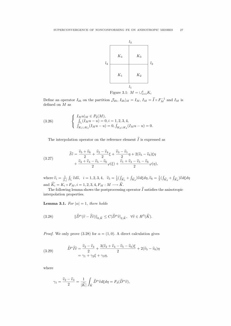
SUPERCONVERGENCE OF NONCONFORMING FE ON ANISOTROPIC MESHES 27
K1 K2
K4 K3
l1
l2
l3
l4
Figure 3.1: M = ∪4i=1Ki
Define an operator I2h on the partition J2h, I2h|M = IM , IM = I F−1M and IM is
defined on M as
(3.26)
IMu|M ∈ P2(M),∫li(IMu− u) = 0, i = 1, 2, 3, 4,∫
K1∪K3(IMu− u) = 0,
∫K2∪K4
(IMu− u) = 0.
The interpolation operator on the reference element I is expressed as
(3.27)I v =
v5 + v6
2+
v2 − v4
2ξ +
v3 − v1
2η + 2(v5 − v6)ξη
+v2 + v4 − v5 − v6
2ϕ(ξ) +
v1 + v3 − v5 − v6
2ϕ(η),
where vi = 1
|li|∫
livds, i = 1, 2, 3, 4, v5 = 1
2 (∫
K1+
∫K3
)vdξdη, v6 = 12 (
∫K2
+∫
K4)vdξdη
and Ki = Ki FM , i = 1, 2, 3, 4, FM : M −→ K.
The following lemma shows the postprocessing operator I satisfies the anisotropicinterpolation properties.
Lemma 3.1. For |α| = 1, there holds
(3.28) ‖Dα(v − I v)‖0,K ≤ C|Dαv|2,K , ∀v ∈ H3(K).
Proof. We only prove (3.28) for α = (1, 0). A direct calculation gives
(3.29)DαI v =
v2 − v4
2+
3(v2 + v4 − v5 − v6)ξ2
+ 2(v5 − v6)η
= γ1 + γ2ξ + γ3η,
where
γ1 =v2 − v4
2=
1
|K|
∫
K
Dαvdξdη = F3(Dαv),
28 S. P. MAO, S. CHEN, AND D. SHI
γ2 =3(v2 + v4 − v5 − v6)
2=
32[12
∫ 1
−1
v(1, η)dη +12
∫ 1
−1
v(−1, η)dη
− 12(∫ 0
−1
∫ 0
−1
v(ξ, η)dξdη +∫ 1
0
∫ 1
0
v(ξ, η)dξdη)
− 12(∫ 0
−1
∫ 1
0
v(ξ, η)dξdη +∫ 1
0
∫ 0
−1
v(ξ, η)dξdη)]
=32[(
12
∫ 0
−1
v(1, η)dη − 12
∫ 0
−1
∫ 0
−1
v(ξ, η)dξdη)
+ (12
∫ 0
−1
v(−1, η)dη − 12
∫ 1
0
∫ 0
−1
v(ξ, η)dξdη)
+ (12
∫ 1
0
v(1, η)dη − 12
∫ 0
−1
∫ 1
0
v(ξ, η)dξdη)
+ (12
∫ 1
0
v(−1, η)dη − 12
∫ 1
0
∫ 1
0
v(ξ, η)dξdη)]
=34[∫ 1
ξ
∫ 0
−1
∫ 0
−1
Dαvdξdηdζ −∫ ξ
−1
∫ 1
0
∫ 0
−1
Dαvdξdηdζ
+∫ 1
ξ
∫ 0
−1
∫ 1
0
Dαvdξdηdζ −∫ ξ
−1
∫ 1
0
∫ 1
0
Dαvdξdηdζ]
= F4(Dαv),
γ3 = 2(v5 − v6) =∫ 0
−1
∫ 0
−1
v(ξ, η)dξdη +∫ 1
0
∫ 1
0
v(ξ, η)dξdη
−∫ 0
−1
∫ 1
0
v(ξ, η)dξdη −∫ 1
0
∫ 0
−1
v(ξ, η)dξdη)
=∫ 0
−1
∫ 0
−1
v(ξ, η)dξdη −∫ 0
−1
v(0, η)dξdη +∫ 0
−1
v(0, η)dξdη −∫ 1
0
∫ 0
−1
v(ξ, η)dξdη
+∫ 1
0
∫ 1
0
v(ξ, η)dξdη −∫ 1
0
v(0, η)dξdη +∫ 1
0
v(0, η)dξdη −∫ 0
−1
∫ 1
0
v(ξ, η)dξdη
=∫ ξ
0
∫ 0
−1
∫ 0
−1
Dαvdξdηdζ −∫ ξ
0
∫ 1
0
∫ 0
−1
Dαvdξdηdζ
+∫ ξ
0
∫ 1
0
∫ 1
0
Dαvdξdηdζ −∫ ξ
0
∫ 0
−1
∫ 1
0
Dαvdξdηdζ
= F5(Dαv).
Where F3, F4, F5 are functionals defined over H2(K) .By Cauchy-Schwarz inequality and the trace theorem, we can show that
|Fi(v)| ≤ C‖v‖1,K ≤ C‖v‖2,K , i = 3, 4, 5,
i.e., Fi, i = 3, 4, 5 are bounded linear functionals on H2(K). Then an applicationof the basic anisotropic interpolation theorem[16] yields the desired result.
Lemma 3.2. The interpolation operator have the following properties:
(3.30) I2hΠhu = I2hu,
(3.30) ‖I2hu− u‖h ≤ Ch2|u|3,Ω,
(3.31) ‖I2hvh‖h ≤ C‖vh‖h,∀vh ∈ Vh.

SUPERCONVERGENCE OF NONCONFORMING FE ON ANISOTROPIC MESHES 29
Proof. (3.30) is obvious and (3.31) can be obtained proceeding along with the samelines of Lemma 2.1. So we only need to prove (3.32).
Thanks to the equivalence of norms over the finite dimensional space, we have
|γi| ≤ C‖Dαvh‖2,K ≤ C‖Dαvh‖0,K , i = 1, 2, 3, ∀vh ∈ Vh.
Then
‖DαI2hvh‖0,K = h−αK (hK1hK2)
12 ‖DαI vh‖0,K
≤ Ch−αK (hK1hK2)
12
3∑
i=1
|γi| ≤ C‖Dαvh‖0,K , ∀vh ∈ Vh.
Hence
‖I2hvh‖h =
∑
K
∑
|α|=1
‖DαI2hvh‖20,K
12
≤ C‖vh‖h,∀vh ∈ Vh,
where the desired result is obtained.Then we can get the following superconvergence theorem easily.
Theorem 3.3. Under the above hypothesis, we have
(3.32) ‖u− I2huh‖h ≤ Ch2(|u|3,Ω + |u|2,Ω + |u|1,Ω).
Proof. Noticing that I2hΠhu = I2hu, then
(3.33)
‖u− I2huh‖h ≤‖u− I2hΠhu‖h + ‖I2h(Πhu− uh)‖h
(3.32)
≤ ‖u− I2hu‖h + C‖Πhu− uh‖h
(3.31)(3.2)
≤ Ch2(|u|3,Ω + |u|2,Ω + |u|1,Ω).
Remark 3.3. We comment that the conventional superconvergence analysis isbased on the quasi-uniform assumption on the meshes. However, here our analysishas avoided the regular assumption and inverse assumption on the meshes, i.e., theconstant C appeared in our estimate is independent of hK/ρK and h/hK .
Remark 3.4. In fact, the meshes Jh is not necessarily as in Figure 3.1 if thequasi-uniform assumption is satisfied. That is to say, for the case Jh is obtainedfrom J2h by dividing each element M of J2h into four different rectangles, wecan still obtain (3.33) with the constant C dependent on hK/ρK and h/hK as inconventional analysis.
4. Extrapolation results
In this section, we assume that αij = Ciδji , where δj
i is the Kronecker index ,Ci = const, i = 1, 2, αi = 0, γ ∈ W 1,∞(Ω) . The meshes consider in this section isregular rectangular meshes.
Lemma 4.1. For any vh ∈ Vh, there holds
(4.1)ah(Πhu− uh, vh) =
∫
Ω
(α11h
2K2
3+
α22h2K1
3
)∂4u
∂x2∂y2vhdxdy
+ O(h3)‖u‖4,Ω‖vh‖h.
30 S. P. MAO, S. CHEN, AND D. SHI
Proof. Let us consider ah(Πhu− u, vh) first,(4.2)
ah(Πhu− u, vh) =∑
K∈Jh
∫
K
(2∑
i=1
αii∂(Πhu− u)
∂xi
∂vh
∂xi+ γ(Πhu− u)vh
)dxdy
= J1 + J2.
It can be checked easily that
(4.3) J1 = 0.
J2 can be decomposed as
(4.4)
J2 =∑
K∈Jh
∫
K
[P0γ(Πhu− u)(vh − P0vh) + P0γP0vh(Πhu− u)
+ (γ − P0γ)(Πhu− u)(vh − P0vh) + (γ − P0γ)(Πhu− u)P0vh]dxdy
= J21 + J22 + J23 + J24.
Then we have
(4.5) J21 ≤ Ch3|u|2,Ω‖vh‖h, J22 = 0, J23 ≤ Ch4|u|2,Ω‖vh‖h,
and by the discrete Poincare inequality (refer to [11, 20, 39, 40]),
(4.6) J24 ≤ Ch3|u|2,Ω‖vh‖0,Ω ≤ Ch3|u|2,Ω‖vh‖h.
So,
(4.7) ah(Πhu− u, vh) ≤ O(h3)|u|2,Ω‖vh‖h.
Now, let us consider ah(u − uh, vh) again, i.e., the consistency error. We onlyneed to prove
(4.8)ah(u− uh, vh) =
∫
Ω
(α11h
2K2
3+
α22h2K1
3
)∂4u
∂x2∂y2vhdxdy
+ O(h3)‖u‖4,Ω‖vh‖h.
For this purpose, we turn back to (3.18) in §3. Set V = ∂U∂x , then
B211 + B4
11 =∫
K
V (vh(xK + hK1, y)− P02vh(xK + hK1, y)) dxdy
= hK1hK2
∫
K
V(vh(1, η)− P02vh(1, η)
)dξdη.
For any fixed vh, we define the functional
T (V ) =∫
K
V(vh(1, η)− P02vh(1, η)
)dξdη − 1
3
∫
K
∂V
∂η
∂vh
∂ηdξdη.
Obviously,
|T (V )| ≤ C‖∂vh
∂η‖0,K‖V ‖2,K .
Hence T ∈ H2(K)′ and ‖T‖ ≤ C‖∂vh
∂η ‖0,K . A detailed calculation shows that
(4.9) T (V ) = 0, ∀V ∈ P1(K).
Then an application of Bramble-Hilbert lemma yields
(4.10) T (V ) ≤ C‖∂vh
∂η‖0,K |V |2,K .

SUPERCONVERGENCE OF NONCONFORMING FE ON ANISOTROPIC MESHES 31
So by the scaling argument and Green’s formula,
(4.11)
B211 + B4
11 ≤ Ch3K‖u‖4,K |vh|1,K +
h2K2
3
∫
K
∂V
∂y
∂vh
∂ydxdy
= O(h3K)‖u‖4,K |vh|1,K +
h2K2
3
∫
K
∂2V
∂y2vhdxdy
+h2
K2
3(∫
l3
−∫
l1
)∂V
∂yvhdx.
Similarly,
(4.12)B1
22 + B322 = O(h3
K)‖u‖4,K |vh|1,K +h2
K1
3
∫
K
∂2V
∂x2vhdxdy
+h2
K1
3(∫
l2
−∫
l4
)∂V
∂xvhdy.
Hence, the summation of K ∈ Jh gives(4.13)
ah(u− uh, vh) =∫
Ω
(α11h
2K2
3+
α22h2K1
3
)∂4u
∂x2∂y2vhdxdy + O(h3)‖u‖4,Ω‖vh‖h
+∑
K∈Jh
(h2
K1
3(∫
l2
−∫
l4
)∂V
∂xvhdy +
h2K2
3(∫
l3
−∫
l1
)∂V
∂yvhdx
).
Then a combination of the obvious result∑
K∈Jh
(h2
K1
3(∫
l2
−∫
l4
)∂V
∂xvhdy +
h2K2
3(∫
l3
−∫
l1
)∂V
∂yvhdx
)= O(h3)‖u‖4,Ω‖vh‖h
implies the desired result, which completes the proof. ¤
Now, we will prove the following error expansions.
Lemma 4.2. There exists a function φ ∈ H2(Ω), such that
(4.14) ‖uh − Ihu− h2φh‖h ≤ Ch3‖u‖4,Ω,
where φh ∈ Vh is a nonconforming finite element projection of φ.
Proof. We define the linear functional
F (v) =∫
Ω
(α11h
2K2
3h2+
α22h2K1
3h2
)∂4u
∂x2∂y2vhdxdy
and consider the following auxiliary problem
(4.15) a(φ, v) = F (v), ∀v ∈ H10 (Ω).
By Lax-Milgram theorem, problem (4.15) exists a solution φ ∈ H2(Ω), and due tothe regularity of elliptic equation
(4.16) ‖φ‖2,Ω ≤ C|u|4,Ω.
Let φh be a nonconforming finite element projection of φ, i.e.,
(4.17)
Find φh ∈ Vh, such that
ah(φh, vh) = F (vh), ∀ vh ∈ Vh.
Then by (4.1), we have
(4.18) ah(uh − Ihu− h2φh, vh) = O(h3)‖u‖4,Ω‖vh‖h.
Taking vh = uh − Ihu− h2φh, then
(4.19) C‖uh − Ihu− h2φh‖2h ≤ ah(uh − Ihu− h2φh, uh − Ihu− h2φh),
32 S. P. MAO, S. CHEN, AND D. SHI
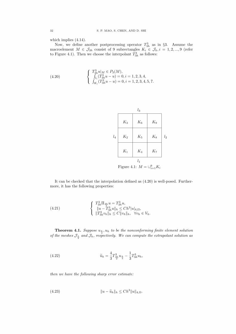
which implies (4.14).Now, we define another postprocessing operator T 3
3h as in §3. Assume themacroelement M ∈ J3h consist of 9 subrectangles Ki ∈ Jh, i = 1, 2, ..., 9 (referto Figure 4.1). Then we choose the interpolant T 3
3h as follows:
(4.20)
T 33hu|M ∈ P3(M),∫li(T 3
3hu− u) = 0, i = 1, 2, 3, 4,∫Ki
(T 33hu− u) = 0, i = 1, 2, 3, 4, 5, 7.
K1
K2
K3
K4
K5
K6
K7
K8
K9
l1
l2
l3
l4
Figure 4.1: M = ∪9i=1Ki
It can be checked that the interpolation defined as (4.20) is well-posed. Further-more, it has the following properties:
(4.21)
T 33hΠ 3h
2u = T 3
3hu,
‖u− T 33hu‖h ≤ Ch3|u|4,Ω,
‖T 33hvh‖h ≤ C‖vh‖h, ∀vh ∈ Vh.
Theorem 4.1. Suppose uh2, uh to be the nonconforming finite element solution
of the meshes Jh2
and Jh, respectively. We can compute the extrapolant solution as
(4.22) uh =43T 3
3h2
uh2− 1
3T 3
3huh,
then we have the following sharp error estimate:
(4.23) ‖u− uh‖h ≤ Ch3‖u‖4,Ω.
SUPERCONVERGENCE OF NONCONFORMING FE ON ANISOTROPIC MESHES 33
Proof. By (4.21) and (4.14), we have(4.24)
‖u− uh‖h = ‖43(u− T 3
3h2
uh2) +
13(T 3
3huh − u)‖h
= ‖43(u− T 3
3h2
Πh2u) +
43(T 3
3h2
Πh2u− T 3
3h2
uh2)
+13(T 3
3huh − T 33hΠhu) +
13(T 3
3hΠhu− u)‖h
= ‖43(u− T 3
3h2
Πh2u)− 4
3T 3
3h2
(uh2−Πh
2u− (
h
2)2φh
2)
+13T 3
3h(uh −Πhu− h2φh) +13(T 3
3hΠhu− u) +h2
3(T 3
3h2
φh2− T 3
3hφh)‖h
≤ C[‖uh2−Πh
2u− (
h
2)2φh
2‖h + ‖u− T 3
3h2
u‖h + ‖uh −Πhu− h2φh‖h
+ ‖T 33hu− u‖h + h2‖T 3
3h2
(φh2− φ)‖h + h2‖T 3
3h2
φ− φ‖h
+ h2‖φ− T 33hφ‖h + h2‖T 3
3h(φ− φh)‖h]
≤ C(h3‖u‖4,Ω + h3‖φ‖2,Ω)
≤ Ch3‖u‖4,Ω
The proof is completed.
Remark 4.1. After we have submitted this paper, we have learned that the su-perconvergence of this element has been studied in [30] by Lin and his collabora-tors. However, the results of this paper are obtained for more general meshes andequations, which will be useful in the numerical analysis of perturbed convection-diffusion-reaction equations where anisotropic meshes are preferred.
5. Numerical experiments
In order to investigate the numerical behavior of the five-node nonconformingelement, we consider the following Dirichlet elliptic boundary problem :
−4u = f, in Ωu = 0, on ∂Ω.
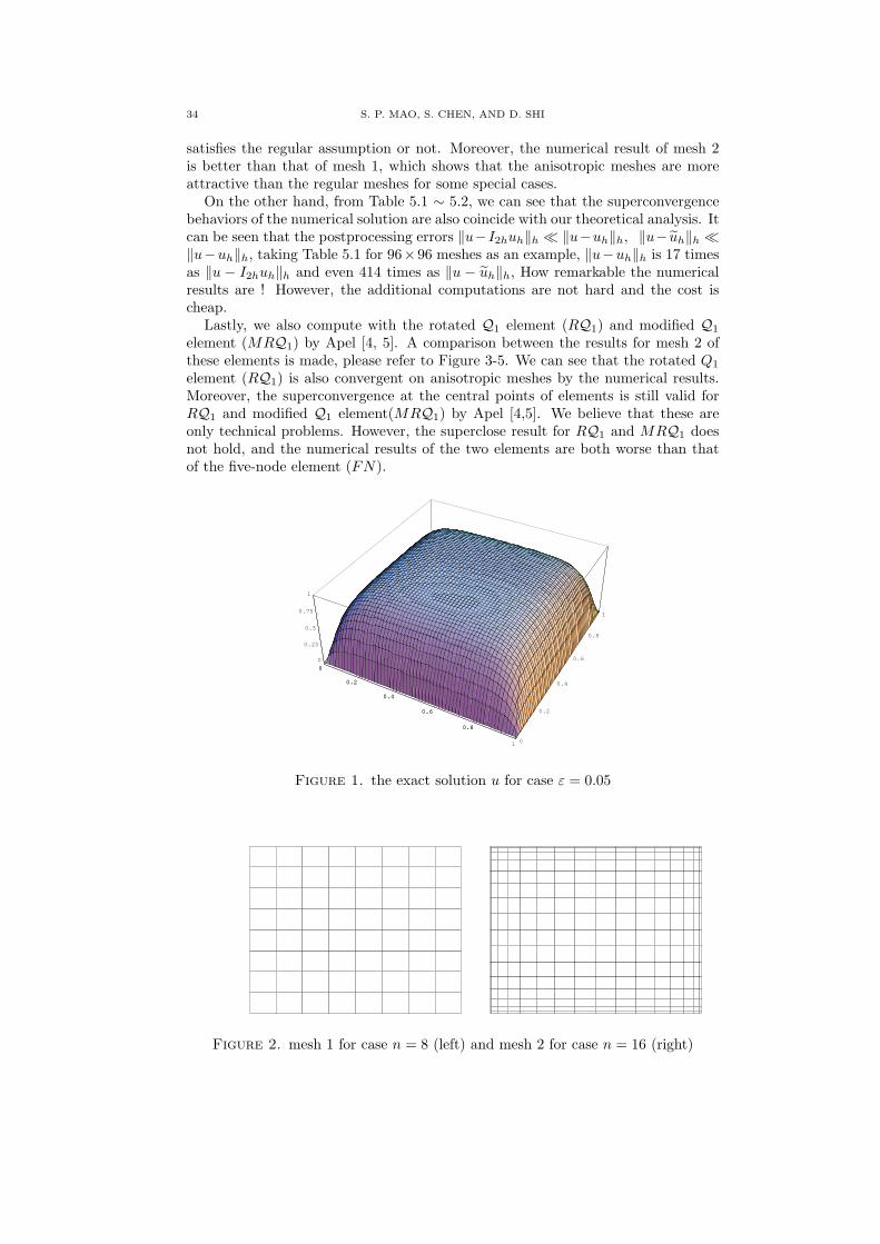
with Ω = [0, 1]× [0, 1], and the right hand side f(x, y) is taken such that u(x, y) =(1 − e(−x(1−x)/ε))(1 − e(−y(1−y)/ε)) (refer to Figure 1 for the case ε = 0.05) is theexact solution, which varies significantly near the boundary of Ω for small ε.
The unit square Ω = [0, 1]× [0, 1] is subdivided in the following two fashions:mesh 1: Subdividing the boundary of Ω into n equal intervals along the x−axis
and y− axis, respectively. The mesh obtained in this way for n = 8 is illustrated inFigure 2 ;
mesh 2: Each edge of Ω is divided into n segments with n + 1 points (1 −cos( iπ
n ))/2, i = 0, 1, ..., n. The mesh obtained in this way for n = 16 is illustrated inFigure 3 ;
The numerical results are listed in Table 5.1∼5.2. Herein, α denotes the conver-
gence order, SEh =
(∑
K∈Jh
|(∇u−∇uh)(OK)|2hK1hK2
) 12
.
From Tables 5.2, we can see that the optimal energy error in norm between u anduh is obtained under large aspect ratio (hK
ρK=
√m2+n2
m ). It shows that the optimalerror estimates are independent of hK , max
K∈Jh
hK/ρK and maxK∈Jh
h/hK, which
means that we can get the same order of error estimates whether the subdivision
34 S. P. MAO, S. CHEN, AND D. SHI
satisfies the regular assumption or not. Moreover, the numerical result of mesh 2is better than that of mesh 1, which shows that the anisotropic meshes are moreattractive than the regular meshes for some special cases.
On the other hand, from Table 5.1 ∼ 5.2, we can see that the superconvergencebehaviors of the numerical solution are also coincide with our theoretical analysis. Itcan be seen that the postprocessing errors ‖u−I2huh‖h ¿ ‖u−uh‖h, ‖u− uh‖h ¿‖u−uh‖h, taking Table 5.1 for 96×96 meshes as an example, ‖u−uh‖h is 17 timesas ‖u − I2huh‖h and even 414 times as ‖u − uh‖h, How remarkable the numericalresults are ! However, the additional computations are not hard and the cost ischeap.
Lastly, we also compute with the rotated Q1 element (RQ1) and modified Q1
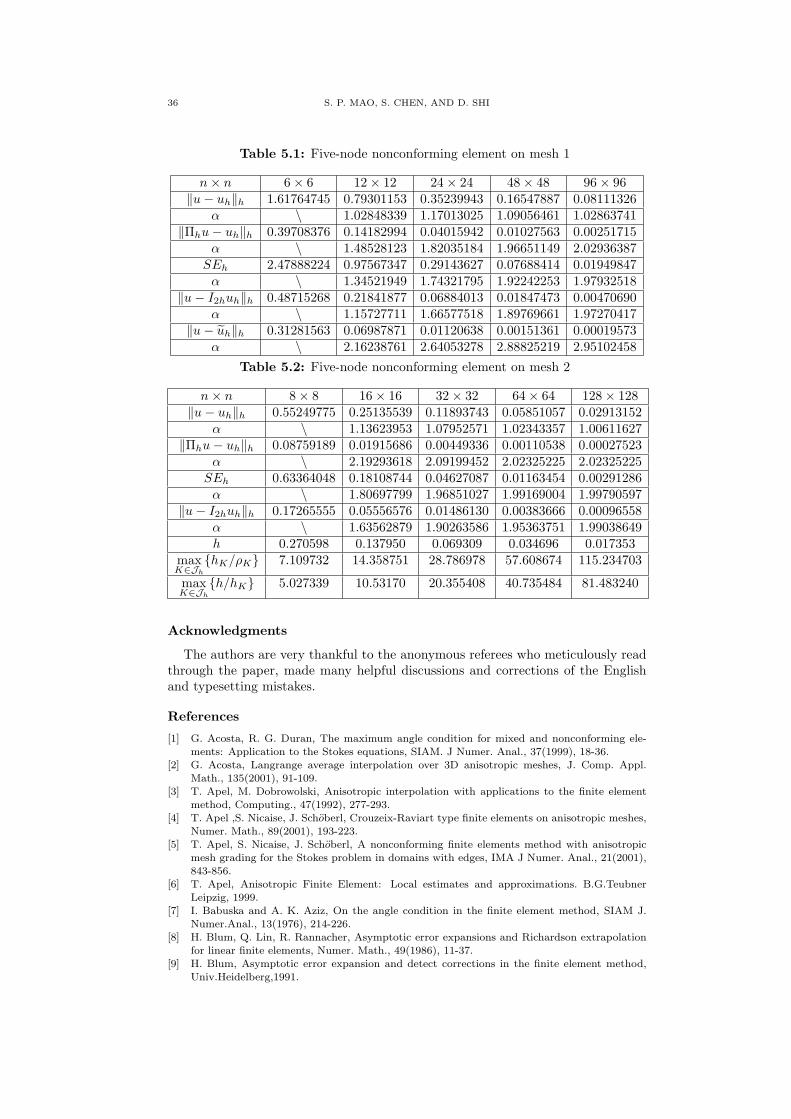
element (MRQ1) by Apel [4, 5]. A comparison between the results for mesh 2 ofthese elements is made, please refer to Figure 3-5. We can see that the rotated Q1
element (RQ1) is also convergent on anisotropic meshes by the numerical results.Moreover, the superconvergence at the central points of elements is still valid forRQ1 and modified Q1 element(MRQ1) by Apel [4,5]. We believe that these areonly technical problems. However, the superclose result for RQ1 and MRQ1 doesnot hold, and the numerical results of the two elements are both worse than thatof the five-node element (FN).
0
0.2
0.4
0.6
0.8
1 0
0.2
0.4
0.6
0.8
1
0
0.25
0.5
0.75
1
0
0.2
0.4
0.6
0.8
Figure 1. the exact solution u for case ε = 0.05
Figure 2. mesh 1 for case n = 8 (left) and mesh 2 for case n = 16 (right)
SUPERCONVERGENCE OF NONCONFORMING FE ON ANISOTROPIC MESHES 35
8·8 16·16 32·32 64·64 128·128
1
2
3
4
MRQ1
RQ1
FN
Figure 3. the numerical results ‖u − uh‖h for FN,RQ1,MRQ1
on mesh 2
8·8 16·16 32·32 64·64 128·128
1
2
3
4
5
MRQ1
RQ1
FN
Figure 4. the numerical results ‖Πhu−uh‖h for FN,RQ1,MRQ1
on mesh 2
8·8 16·16 32·32 64·64 128·128
0.5
1
1.5
2
2.5
3
MRQ1
RQ1
FN
Figure 5. the numerical results SEh for FN, RQ1, MRQ1 onmesh 2
36 S. P. MAO, S. CHEN, AND D. SHI
Table 5.1: Five-node nonconforming element on mesh 1
n× n 6× 6 12× 12 24× 24 48× 48 96× 96‖u− uh‖h 1.61764745 0.79301153 0.35239943 0.16547887 0.08111326
α \ 1.02848339 1.17013025 1.09056461 1.02863741‖Πhu− uh‖h 0.39708376 0.14182994 0.04015942 0.01027563 0.00251715
α \ 1.48528123 1.82035184 1.96651149 2.02936387SEh 2.47888224 0.97567347 0.29143627 0.07688414 0.01949847α \ 1.34521949 1.74321795 1.92242253 1.97932518
‖u− I2huh‖h 0.48715268 0.21841877 0.06884013 0.01847473 0.00470690α \ 1.15727711 1.66577518 1.89769661 1.97270417
‖u− uh‖h 0.31281563 0.06987871 0.01120638 0.00151361 0.00019573α \ 2.16238761 2.64053278 2.88825219 2.95102458
Table 5.2: Five-node nonconforming element on mesh 2
n× n 8× 8 16× 16 32× 32 64× 64 128× 128‖u− uh‖h 0.55249775 0.25135539 0.11893743 0.05851057 0.02913152
α \ 1.13623953 1.07952571 1.02343357 1.00611627‖Πhu− uh‖h 0.08759189 0.01915686 0.00449336 0.00110538 0.00027523
α \ 2.19293618 2.09199452 2.02325225 2.02325225SEh 0.63364048 0.18108744 0.04627087 0.01163454 0.00291286α \ 1.80697799 1.96851027 1.99169004 1.99790597
‖u− I2huh‖h 0.17265555 0.05556576 0.01486130 0.00383666 0.00096558α \ 1.63562879 1.90263586 1.95363751 1.99038649h 0.270598 0.137950 0.069309 0.034696 0.017353
maxK∈Jh
hK/ρK 7.109732 14.358751 28.786978 57.608674 115.234703
maxK∈Jh
h/hK 5.027339 10.53170 20.355408 40.735484 81.483240
Acknowledgments
The authors are very thankful to the anonymous referees who meticulously readthrough the paper, made many helpful discussions and corrections of the Englishand typesetting mistakes.
References
[1] G. Acosta, R. G. Duran, The maximum angle condition for mixed and nonconforming ele-ments: Application to the Stokes equations, SIAM. J Numer. Anal., 37(1999), 18-36.
[2] G. Acosta, Langrange average interpolation over 3D anisotropic meshes, J. Comp. Appl.Math., 135(2001), 91-109.
[3] T. Apel, M. Dobrowolski, Anisotropic interpolation with applications to the finite elementmethod, Computing., 47(1992), 277-293.
[4] T. Apel ,S. Nicaise, J. Schoberl, Crouzeix-Raviart type finite elements on anisotropic meshes,Numer. Math., 89(2001), 193-223.
[5] T. Apel, S. Nicaise, J. Schoberl, A nonconforming finite elements method with anisotropicmesh grading for the Stokes problem in domains with edges, IMA J Numer. Anal., 21(2001),843-856.
[6] T. Apel, Anisotropic Finite Element: Local estimates and approximations. B.G.TeubnerLeipzig, 1999.
[7] I. Babuska and A. K. Aziz, On the angle condition in the finite element method, SIAM J.Numer.Anal., 13(1976), 214-226.
[8] H. Blum, Q. Lin, R. Rannacher, Asymptotic error expansions and Richardson extrapolationfor linear finite elements, Numer. Math., 49(1986), 11-37.
[9] H. Blum, Asymptotic error expansion and detect corrections in the finite element method,Univ.Heidelberg,1991.

SUPERCONVERGENCE OF NONCONFORMING FE ON ANISOTROPIC MESHES 37
[10] S. C. Brenner, L. R. Scott, The mathematical theory of finite element methods, New York,Springer-Verlag, 1994.
[11] S. C. Brenner, Poincare-Friedrichs inequalities for piecewise H1 functions, SIAM J. Nu-mer.Anal., 41(2003), 306-324.
[12] Z. Q. Cai, J. Douglas Jr., X. Ye, A stable nonconforming quadrilateral finite element methodfor the stationary Stokes and Navier-Stokes equations. Calcolo, 36(1999), 215-232.
[13] P. G. Ciarlet, The Finite Element Method for Elliptic Problems, North-Holland, Amsterdam,New York, Oxford, 1978.
[14] C. M. Chen and Y. Q. Huang, High accuracy theory of finite element methods (in Chinese),Hunan Science Press, P.R. China, 1995.
[15] H. S. Chen and B. Li, Superconvergence analysis and error expansion for the Wilson noncon-forming finite element, Numer. Math., 69(1994), 125-140.
[16] S. C. Chen, D. Y. Shi, Y. C. Zhao, Anisotropic interpolation and quasi-Wilson element fornarrow quadrilateral meshes, IMA J Numer. Anal., 24(2004), 77-95.
[17] S. C. Chen, Y. C. Zhao, D. Y. Shi, Anisotropic interpolations with application to noncon-forming elements, Appl Numer.Math., 49 (2004), 135-152.
[18] W. J. Chen, X. L. Yang, Variational basement and geometric inviarants of generalized con-forming element,Comput. struct. Mech. Appl., 13(1992), 245-252.
[19] E. Creuse, G. Kunert, S. Nicaise, A posterior error estimation for the Stokes problem:Anisotropic and isotropic discretizations. Preprint-Reihe des Chemnitzer SFB 393, 2003.
[20] V. Dolejsi, M. Feistauer and J. Felcman, On the Friedrichs inequality for nonconforming finiteelements, Numer. Func. Anal and Opti., 20(1999), 427-437.
[21] J. Douglas, J. E. Santos, D. Sheen and X. Ye, Nonconforming Galerkin methods based onquadrilateral elements for second order elliptic problems, RAIRO Model. Math. Anal. Numer., 33(4)(1999), 747-770.
[22] R. G. Duran, Error estimates for narrow 3D finite elements, Math Comp., 68 (1999), 187-199.[23] R. G. Duran, A. L. Lombardi, Error estimates on anisotropic Q1 elements for functions in
weighted sobolev spaces, Math. Comp., 74 (2005), 1679-1706.[24] H. D. Han, Nonconforming elements in the mixed finite element method, Journal of Compu-
tational Mathematics, 2(1984), 223-233.[25] P. Jamet, Estimations d’erreur pour des elements finis droits presque degeneres, RAIRO
Anal.Numer., 10(1976), 46-61.
[26] M. Krizek and P. Neittaanmaki, On superconvergence techniques, Acta Applicandae Math-ematicae, 9(1987), 175-198.
[27] P. Lascaux and P. Lesaint, Some noncomforming finite element for the plate bending problem,RAIRO, Anal. Numer. R-1(1975), 9-53.
[28] J. Lazaar, Serge Nicaise, A nonconforming finite elements method with anisotropic mesh grad-ing for the incompressible Navier-Stokes equations in domains with edges. Calcolo, 39(2002),123-168.
[29] Q. Lin, N. Yan, The Construction and Analysis of High Efficient Elements, Hebei UniversityPress,1996. (in Chinese).
[30] Q. Lin, L. Tobiska and A. Zhou, On the superconvergence of nonconforming low order finiteelements applied to the Poisson equation, IMA J Numer. Anal., 25(2005), 160-181.
[31] S. P. Mao, S. C. Chen, H. X. Sun, A quadrilateral, anisotropic, superconvergent nonconform-ing double set parameter element, Appl. Numer. Math., 56 (2006), 937-961.
[32] P. B. Ming, Y. Xu and Z. C. Shi, Superconvergence studies of quadrilateral nonconformingrotated Q1 elements, International Journal of Numerical Analysis and Modeling, 3(2006),322-332.
[33] J. Nitsche, L∞-error analysis for finite elements, In the Mathematics of Finite Elements andApplications III (Whiteman, J.R.,ed.) 173-186; Academic Press, New York.1979.
[34] R. Rannacher and S. Turek, Simple nonconforming quadrilateral stokes element, Numer.Meth. PDE 8(1992), 97-111.
[35] R. Rannacher, Richardson extrapolation with finite elements, Numeric Techniques in Con-tinum Mechanics, Ind GAMM- Seminar, Kiel (W.Hackbusch and C.Witsch, eds) (1986), 90-101.
[36] R. Rannacher, Extrapolations techniques in the finite element method (A Survey), SummerSchool on Numerical Analysis, Helsinki, Univ. of Tech., MATC7, (1988) 80-113.
[37] N. Al Shenk, Uniform error estimates for certain narrow Lagrange finite elements, Math.Comp., 63(1994), 105-119.
[38] D. Y. Shi, S. P. Mao and S. C. Chen, An anisotropic nonconforming finite element withsome superconvergence results, Journal of Computational Mathematics, 23 (2005), 261-274.
[39] Z. C. Shi and B. Jiang, A new superconvergence property of Wilson nonconforming finiteelement, Numer math., 78 (1997), 259-268.

38 S. P. MAO, S. CHEN, AND D. SHI
[40] Z. C. Shi, The F-E-M-Test for convergence of nonconforming elements, Math. Comp.,49(1987), 391-405.
[41] F. Stummel, Basic compactness properties of nonconforming and hybrid finite element spaces,RAIRO. Anal. Numer., 14(1980), 81-115.
[42] R. Teman, Navier-Stokes Equation: Theorey and Numerical Analysis, North-Holland(3ed),1983.
[43] L. B. Wahlbin, Superconvergence in Galerkin Finite Element Methods, Lecture Notes inMathematicas, Vol.1605, Springer, Berlin, 1995.
[44] J. P. Wang and X. Ye, Superconvergence of finite element approximations for the Stokesproblem by least squares surface fitting, SIAM J. Numer. Anal., 39 (2001), 1001-1013.
[45] A. Zenisek, M. Vanmaele, Applicability of the Bramble-Hilbert lemma in interpolation prob-lems of narrow quadrilateral isoparametric finite elements, J. Comp Appl Math., 65(1995),109-122.
Institute of Computational Mathematics and Scientific/Engineering Computing, Academy ofMathematics and System Science, Chinese Academy of Science, PO Box 2719, Beijing, 100080,People’s Republic of China
E-mail : [email protected]
URL: http://lsec.cc.ac.cn/maosp
Department of Mathematics, Zhengzhou University, Zhengzhou, 450052, People’s Republic ofChina
E-mail : [email protected]
Department of Mathematics, Zhengzhou University, Zhengzhou, 450052, People’s Republic ofChina
E-mail : [email protected]