volume 8 semantic map geometry: two issue 1 approaches

Semantic Map Geometry: Two Approaches

Joost Zwarts

Utrecht Institute of Linguistics OTS

doi: 10.1349/PS1.1537-0852.A.357

url: http://journals.dartmouth.edu/cgi-bin/WebObjects/Journals.woa/1/xmlpage/1/article/357

Volume 8Issue 12010

Linguistic DiscoveryPublished by the Dartmouth College Library

Copyright to this article is held by the authors.ISSN 1537-0852

linguistic-discovery.dartmouth.edu

Linguistic Discovery 8.1:377-395

Semantic Map Geometry: Two Approaches

Joost Zwarts

Utrecht Institute of Linguistics OTS

This paper discusses two ways in which the geometry of a semantic map can be defined: on the

basis of a set of cross-linguistic data or on the basis of a semantic analysis of the meanings

involved. I will argue that under a purely “data-driven” approach certain important aspects of

contiguity in semantic maps, like exceptions and family resemblance structure, remain unclear

and that we can get more insight into these aspects when working from a semantically defined

geometry. The two approaches can complement each other in the use of semantic maps.

A semantic map is a ―spatial‖ representation of the ways in which a set of linguistic meanings

hangs together. More similar meanings are closer together on the map, while less similar

meanings are further apart. Underlying the spatial representation is a particular geometry that

defines how similarities correspond to spatial distances or connections, either in graphs or in

MDS. This paper is about two different ways in which the geometry of a semantic map can be

derived and applied, working from cross-linguistic data or working from a semantic model.

Because these two approaches both have their limitations, it follows that they can complement,

inform, and correct each other.

After a brief introduction to the notion of semantic maps in section 1, I will explain the two

approaches in section 2 and some of the limitations and pitfalls in section 3 and section 4.

Section 5 concludes the paper.

1. Semantic Map = Lexical Matrix + Conceptual Space

Building on earlier distinctions in Croft (2001) and Haspelmath (2003), I will assume that a

semantic map for a particular domain consists of two parts: a lexical matrix and a conceptual

space. A conceptual space is a geometrically ordered set of meanings, typically a graph, like

Haspelmath‘s (1997a) well-known space of indefinite meanings:

(1)

specific

known

(1)

specific

unknown

(2)

irrealis

non-specific

(3)

question

(4)

conditional

(5)

indirect

negation

(6)

comparative

(8)

direct

negation

(7)

free

choice

(9)

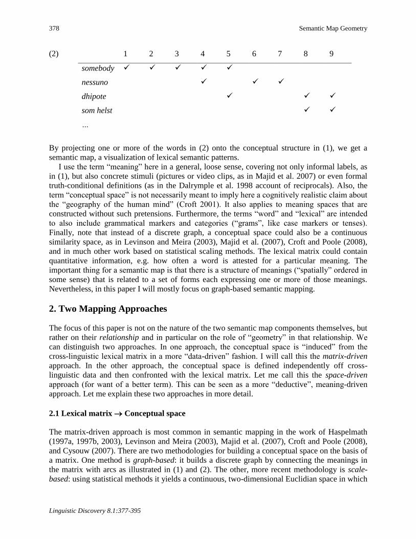
The lexical matrix in its simplest form is a table which shows for each word in a set of words (or

grams) which meanings (or functions) from the conceptual space it can express. Here is a small

fragment of the lexical matrix for indefinite pronouns in Haspelmath (1997a):

378 Semantic Map Geometry


(2) 1 2 3 4 5 6 7 8 9

somebody

nessuno

dhipote

som helst

…

By projecting one or more of the words in (2) onto the conceptual structure in (1), we get a

semantic map, a visualization of lexical semantic patterns.

I use the term ―meaning‖ here in a general, loose sense, covering not only informal labels, as

in (1), but also concrete stimuli (pictures or video clips, as in Majid et al. 2007) or even formal

truth-conditional definitions (as in the Dalrymple et al. 1998 account of reciprocals). Also, the

term ―conceptual space‖ is not necessarily meant to imply here a cognitively realistic claim about

the ―geography of the human mind‖ (Croft 2001). It also applies to meaning spaces that are

constructed without such pretensions. Furthermore, the terms ―word‖ and ―lexical‖ are intended

to also include grammatical markers and categories (―grams‖, like case markers or tenses).

Finally, note that instead of a discrete graph, a conceptual space could also be a continuous

similarity space, as in Levinson and Meira (2003), Majid et al. (2007), Croft and Poole (2008),

and in much other work based on statistical scaling methods. The lexical matrix could contain

quantitative information, e.g. how often a word is attested for a particular meaning. The

important thing for a semantic map is that there is a structure of meanings (―spatially‖ ordered in

some sense) that is related to a set of forms each expressing one or more of those meanings.

Nevertheless, in this paper I will mostly focus on graph-based semantic mapping.

2. Two Mapping Approaches

The focus of this paper is not on the nature of the two semantic map components themselves, but

rather on their relationship and in particular on the role of ―geometry‖ in that relationship. We

can distinguish two approaches. In one approach, the conceptual space is ―induced‖ from the

cross-linguistic lexical matrix in a more ―data-driven‖ fashion. I will call this the matrix-driven

approach. In the other approach, the conceptual space is defined independently off cross-

linguistic data and then confronted with the lexical matrix. Let me call this the space-driven

approach (for want of a better term). This can be seen as a more ―deductive‖, meaning-driven

approach. Let me explain these two approaches in more detail.

2.1 Lexical matrix Conceptual space

The matrix-driven approach is most common in semantic mapping in the work of Haspelmath

(1997a, 1997b, 2003), Levinson and Meira (2003), Majid et al. (2007), Croft and Poole (2008),

and Cysouw (2007). There are two methodologies for building a conceptual space on the basis of

a matrix. One method is graph-based: it builds a discrete graph by connecting the meanings in

the matrix with arcs as illustrated in (1) and (2). The other, more recent methodology is scale-

based: using statistical methods it yields a continuous, two-dimensional Euclidian space in which

Zwarts 379


the meanings are represented as points. I will focus here on the graph-based version of this

approach, using the example in (1) and (2), but the general idea of starting with the data and

building a conceptual space applies to the scale-based approach as well.

Where the lines are drawn in (1) is entirely determined by the linguistic data in (2), without

any consideration of what we might already know about the meanings themselves. The idea is, in

fact, that we can learn how a set of meanings hangs together from what the words do. Note,

however, that this approach still makes important analytical and theoretical assumptions about

the number and kind of meanings to distinguish for a particular domain. The point is that, in

principle, no assumptions are made about how these meanings relate to each other, i.e. how they

are ―geometrically‖ organized.

In the matrix-driven approach, a graph is constructed on the basis of an important principle

called contiguity or connectivity. The task is to construct an undirected graph G in which every

word in the lexical matrix covers a connected subgraph and in which, furthermore, G does not

contain a subgraph G in which this is also the case. So, we are looking for a graph of meanings

that has as few links as possible while still guaranteeing connectivity for every word. In (1),

through the connections between meanings 4 and 6 and between 6 and 7, the word nessuno

covers a connected subgraph. However, a word with the meanings 3, 4, and 7 would not have

connectivity in (1) because there is no arc between 3 or 4 on the one hand and 7 on the other

hand. If we were to find such a word, then the graph would have to be extended with such an arc

in order to ensure that there is a connected subgraph for the word with meanings {3, 4, 7}.

The graph in (1) embodies a claim as to which of the indefinite meanings 1 to 9 are closer to

each other. ―Specific known‖ is closer to ―specific unknown‖ than to any other meaning, and it is

quite far away from ―direct negation‖. Roughly speaking, this is because there are words

including only meaning 1 and 2, but no word has been found including 1 and 7, without also

including the meanings in between, more precisely, the meanings on a path leading from 1 to 7.

We can define the distance between two meanings A and B in a graph as the length of the

shortest path connecting A and B. So, in (1), the distance between meanings 1 and 7 is five arcs

and the distance between 4 and 9 is three arcs.

The idea that distance in the conceptual space reflects similarity between meanings as defined

by the lexical matrix is also found in the statistical approaches, as in the study of cutting and

breaking verbs by Majid et al.: ―Correspondence analysis produces a ‗semantic map‘ that plots

stimuli (here, the video clips) in a multidimensional space, with the distance between any two

stimuli reflecting their degree of similarity (here, the degree to which speakers of various

languages used the same verb to describe them), calculated across the data set as a whole,‖

(Majid et al. 2007:141). In such an approach, a word will also correspond to a contiguous area on

the map. So, importantly, whether we arrive at a conceptual space through ―correspondence

analysis‖ or by drawing a graph, in both cases we derive the ―geometric‖ structure entirely from

the given lexical matrix.

2.2 Conceptual space Lexical matrix

Instead of constructing a conceptual space from a lexical matrix, it is also possible to take an

existing conceptual space and investigate how words are mapped onto it. The classic example of

this approach is the study of color terms (from the seminal work by Berlin and Kay 1969 to

recent work, Regier et al. 2007). The organization of color chips into a color space with its

dimensions of hue, saturation, and brightness is not derived from color terms in languages across



the world, but independently defined on the basis of physical or psychological considerations,

without taking into account how languages differentially name those values. We can then study

how languages use words to carve up this color space, and we can test whether the terms are

actually contiguous or convex in it. One of the central claims in Gärdenfors‘s (2000) theory of

conceptual spaces is that color terms in fact correspond to convex regions. We can also study

how the structure of the space determines other properties of color terms over and above

convexity or connectivity, like organization around focal colors.

There are some other examples in the literature where a conceptual structure is given

relatively independent of linguistic data. In the study of body part terminology, the human body

already provides a partial geometry which is obviously relevant for the lexical patterns that we

find. Kinship is another domain where a conceptual structure, based on notions like descent,

gender, and marriage, can be constructed independently of various terminologies used for kin. In

such a structure, the kinship type of ―father‖ is closer to ―father‘s brother‖ than to ―mother‘s

brother‖ under any conceptual analysis of these types. It is no surprise then that there are uncle

terminologies that use the same term for ―father‖ and ―father‘s brother‖, excluding ―mother‘s

brother‖, but there are no terminologies in which ―father‖ and ―mother‘s brother‖ are taken

together (Greenberg 1966).

Crucially, the domains of color, body parts, and kinship come with geometric notions of

distance and ―betweenness‖ even before we look at the lexicon, and we can study whether and

how this prior geometry influences the structure of the lexicon. This does not mean that the right

or the only geometry for understanding semantic patterns easily presents itself. For example, the

anatomical distance between fingers and toes does not explain why languages can sometimes use

the same word for both, indicating that the conceptual space of the human body is more than just

the ―anatomical space‖. It also takes into account anatomical similarities that exist between

different body parts. In the same way, ―kinship space‖ might not be simply a genealogical tree

structure but a space defined over such dimensions as generation, gender, and collateral distance.

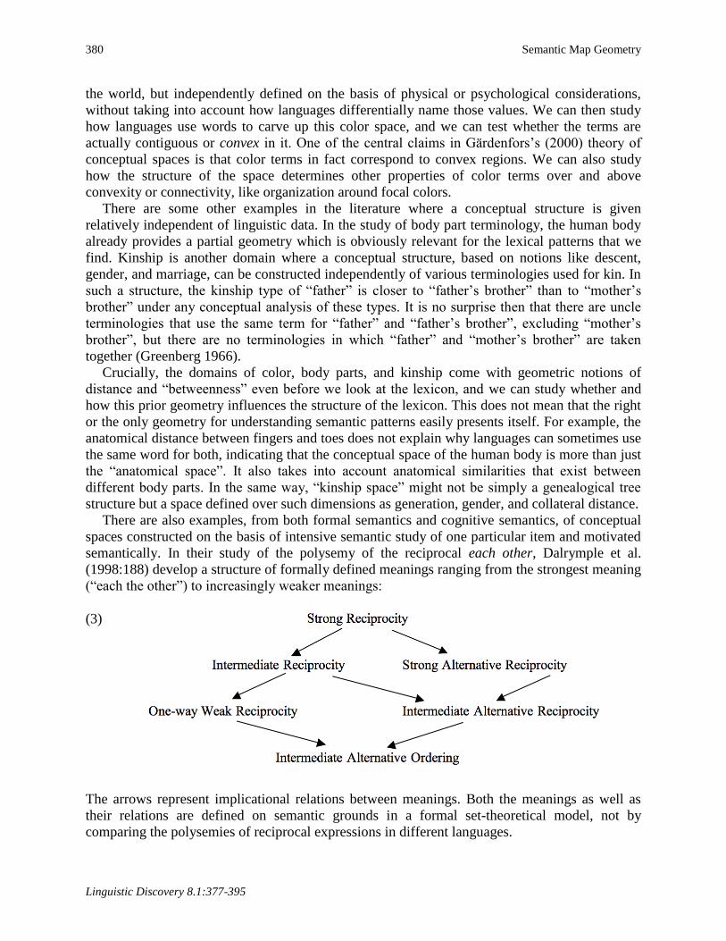
There are also examples, from both formal semantics and cognitive semantics, of conceptual

spaces constructed on the basis of intensive semantic study of one particular item and motivated

semantically. In their study of the polysemy of the reciprocal each other, Dalrymple et al.

(1998:188) develop a structure of formally defined meanings ranging from the strongest meaning

(―each the other‖) to increasingly weaker meanings:

(3)

The arrows represent implicational relations between meanings. Both the meanings as well as

their relations are defined on semantic grounds in a formal set-theoretical model, not by

comparing the polysemies of reciprocal expressions in different languages.

Zwarts 381


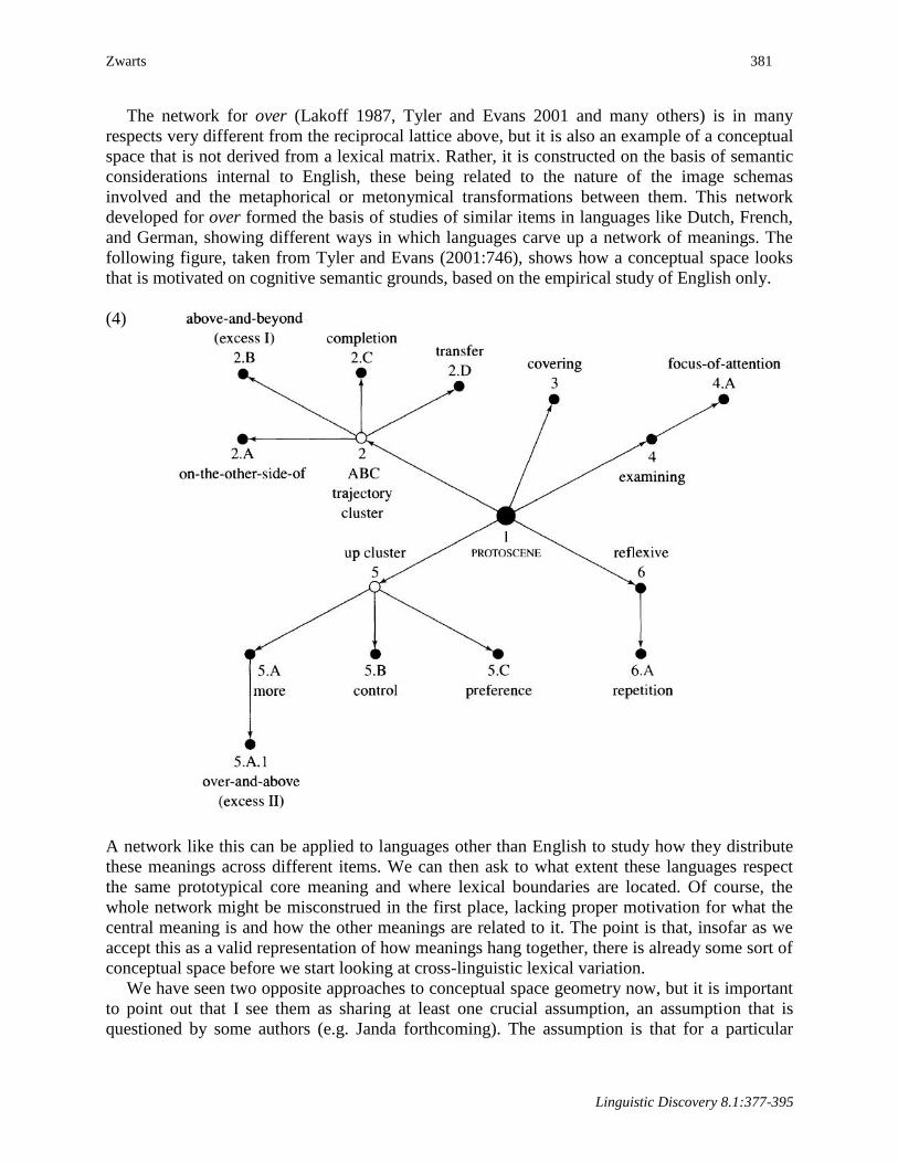
The network for over (Lakoff 1987, Tyler and Evans 2001 and many others) is in many

respects very different from the reciprocal lattice above, but it is also an example of a conceptual

space that is not derived from a lexical matrix. Rather, it is constructed on the basis of semantic

considerations internal to English, these being related to the nature of the image schemas

involved and the metaphorical or metonymical transformations between them. This network

developed for over formed the basis of studies of similar items in languages like Dutch, French,

and German, showing different ways in which languages carve up a network of meanings. The

following figure, taken from Tyler and Evans (2001:746), shows how a conceptual space looks

that is motivated on cognitive semantic grounds, based on the empirical study of English only.

(4)

A network like this can be applied to languages other than English to study how they distribute

these meanings across different items. We can then ask to what extent these languages respect

the same prototypical core meaning and where lexical boundaries are located. Of course, the

whole network might be misconstrued in the first place, lacking proper motivation for what the

central meaning is and how the other meanings are related to it. The point is that, insofar as we

accept this as a valid representation of how meanings hang together, there is already some sort of

conceptual space before we start looking at cross-linguistic lexical variation.

We have seen two opposite approaches to conceptual space geometry now, but it is important

to point out that I see them as sharing at least one crucial assumption, an assumption that is

questioned by some authors (e.g. Janda forthcoming). The assumption is that for a particular



domain there is one universal conceptual space which is somehow valid for all natural languages.

Haspelmath‘s indefinite pronoun space in (1) is a space in which all languages necessarily locate

their indefinite pronouns. It simply does not leave open the option that there are languages which

map their pronouns to a different space with different meanings or differently organized

meanings. In color terminology research, languages are also compared on the basis of one and

the same space of colors. Languages can only differ in the way they organize this color space,

not in the color spaces themselves, even if they make only very few distinctions. In other words:

languages can differ in their semantic maps, not in their conceptual spaces.

It is possible to conceive of a different setup in which each language has its own conceptual

space for a particular domain. Janda suggests that a language without gender distinctions in its

pronominal system (like Finnish) has a ―flat gender landscape‖ (i.e. conceptual gender space) in

contrast to languages with gender distinctions. In this case there is no distinction between a

language-specific semantic map and universal conceptual space. Each language has its own

specific conceptual spatialization of a particular domain, and we need special mappings between

conceptual spaces to see how similar or different languages are. Obviously, linguistic

comparison becomes a much more difficult job under these assumptions. In the semantic map

approach (whether space-driven or matrix-driven), comparison is possible exactly because

languages share the same conceptual space (either a priori or a posteriori). I take this to be a

methodological assumption rather than an ontological and cognitive one. It could very well be

that we ultimately need to reinterpret each language-specific semantic map as reflecting the

conceptual space of that particular language, merging meanings that are never distinguished by

that language. However, for the purposes of this paper I will leave the universalist assumption of

conceptual spaces for what it is. The focus here is on the distinction between the two directions

of analysis.

It is also important to stress that even though both approaches seem to work in opposite

directions, it is not the case that the matrix-driven approach is purely data-driven, inductive, a

posteriori, and empirical while the space-driven approach is theory-driven, deductive, and a

priori. As always, there is a combination of theoretical assumptions and empirical data. For this

paper, the crucial difference lies in the way relations between meanings are treated: as derived

from semantic considerations or from cross-linguistic data.

I will first discuss some problems with the space-driven approach that have partially

motivated the matrix-driven approach, the latter being characteristic for much semantic map

work. After that I will demonstrate that a purely matrix-driven approach raises some important

questions, strongly suggesting that we need both approaches to complement each other.

3. Problems with a Space-Driven Approach

In a sense, the domains of color, body, and kinship are easy examples of conceptual spaces

because they carry much of their structure on their sleeves. The problem is that for many

(especially more abstract) domains it is not at all easy to find an a priori conceptual geometry.

Consider the graph in (1). Even though a lot of semantic work has been done in the area of

reference, quantification, questions, negation, polarity, and modality, the body of insight does not

yet straightforwardly deliver us a network of meaning relations comparable to (1) purely on the

basis of what we know about the meanings themselves. This is true for many of the conceptual

spaces that semantic map typologists have worked on in relation to case, aspect, tense, modality,

and evidentiality. It is often very hard to come up with a unique structure of meanings for a

Zwarts 383


particular domain motivated on semantic grounds. Existing theories conflict with each other, or

they offer only a partial view. The word over is a typical case. There is disagreement among

various authors about the way the network for over should be organized, what its focal meaning

is, and how the various meanings are related, leading to a still growing body of publications on

the subject ever since Brugman‘s original work (Brugman 1988, Lakoff 1987, Dewell 1994,

Sandra and Rice 1995, Tyler and Evans 2001 only being some of the publications on this word).

In the absence of strong independent semantic evidence for structuring a domain in a particular

way, it is natural that in such a situation we would turn to cross-linguistic data and let those data

(i.e. the lexical matrix) tell us what the underlying conceptual structure is. This is what motivates

the semantic map approach.

Another problem with the space-driven approach is that an a priori conceptual geometry

might actually bias our research in a particular way and hinder us from finding patterns and

dimensions in other languages. It is all too easy to assume that we have a universally valid

structure, based on one language (typically English), while the richness of a wider variety of

languages does not really fit on the map. This is where the matrix-driven approach has an

important heuristic value. It doesn‘t fix itself to any specific assumptions about sense relations,

what the dimensions are of a semantic space, or where the core meanings are—all of this based

on studying a single language. Instead it aims at discovering these aspects for a particular domain

from what many different languages tell us. This heuristic advantage is also strongly connected

to the visualization and spatialization aspect of the semantic map approach. It is possible to view

a semantic map as offering just one particular spatialization of the data among many different

options, helping the analyst to find his way. This view is expressed for instance by Wälchli

(2007), who emphasizes that there ―are always different possible ways of analysis, each with its

particular advantages and disadvantages. Semantic maps will thus never reflect the semantic

space, if there is such a thing at all.‖ (Wälchli 2007:47, see Cysouw 2007 for similar remarks).

There are other problems with the space-driven approach in general and with specific

instantiations of it, which have led to a matrix-driven approach. However, I would now like to

turn to some considerations that show that the matrix-driven approach in its purest form faces

some interesting questions. My argumentation is restricted to graph-based semantic maps and the

important property of contiguity, but I believe the conclusions are valid for scale-based

approaches too in a more general sense that remains to be worked out.

4. Two Problems with a Matrix-Driven Approach

4.1 Exceptions to contiguity

As we saw in section 2.1, there is an important principle in matrix-driven mapping which has

been indicated with various terms in the literature: connectivity, contiguity, convexity,

coherence, or compactness. Roughly speaking, the idea is that the meanings of a word are always

close together in a conceptual space, forming one cluster. In the graph-based approach a word

corresponds to a connected subgraph. There are no gaps in a word, and a word is never split into

two separate parts located in different corners of the conceptual space. It is this principle of

contiguity that allows us to build a conceptual graph or space on the basis of a lexical matrix. As

a result, the principle is an implicit part of the procedure for building a conceptual graph or

space. This has some important limitations for understanding the principle itself, its nature, and

the way it applies.



First, because of its constitutive role in building a space, contiguity cannot be directly tested

as a hypothesis about the way words distribute themselves over a conceptual space. Neither does

it allow for exceptions. Suppose we have the following very small lexical matrix, with two

words, A and B, and the meanings 1, 2, 3:

(5) 1 2 3

A

B

Given contiguity, this matrix leads to the following graph:

(6)

1 2 3

Suppose now that we discover another word C in some language that has the meanings 1 and 3.

The logic of the matrix-driven approach forces us to revise the space in the following way,

guaranteeing that all three words now correspond to a connected subgraph:

(7)

1 2

3

There is no way to treat word C as an exception to contiguity, i.e. as a discontinuous word, for

whatever reason. Exceptions can‘t be recognized in the matrix-driven approach.

That this is not an academic example is illustrated by the modality map of van der Auwera

and Plungian (1998) and van der Auwera et al. (2009). For the possibility part, the conceptual

space corresponding to this map can be represented as follows:1

1I have adapted the representation of van der Auwera and Plungian and van der Auwera et al. to make it more

similar to Haspelmath‘s representation. They represent meanings by means of Venn-diagram-like ovals and subtype

relations by means of inclusion.

Zwarts 385


(8)

participant-

internal

participant-

external

deontic

optative

epistemic

concessive

Van der Auwera‘s maps are special because they encode the direction of grammaticalization in

the map by means of arrows and also allow one modality to be a subtype of another modality

(represented here by the dotted arrow). So, concessive modality is treated as an instance of the

more general epistemic modality. For extensive motivation and examples I refer the reader to

van der Auwera and Plungian (1998) and van der Auwera et al. (2009).

What is important now is that these authors argue that there are examples of discontiguity on

the modal map. One example is Dutch mogen, which is used for deontic (9a), concessive (9b),

and optative (9c), but not for participant-external (9d) and epistemic (9e):2

(9) a. Ik mag gaan.

I may go

‗I may go.‘

b. Hij mag slim zijn, sympathiek is hij niet.

he may clever be nice is he not

‗He may be clever, but he is not nice.‘

c. Moge hij honderd jaar leven!

may he hundred year live

‗May he live a hundred years!‘

d. * Om naar het station te gaan, mag je bus 66 nemen. to to the station to go may you bus 66 Take

‗To get to the station, you may take bus 66.‘

e. * Hij mag thuis zijn, ik weet het niet. he may home be, I know It not

‗He may be home, I don‘t know.‘

2Examples taken from van der Auwera et al. (2009:6-7).



When we indicate the meanings of mogen on the modal map, we can see that they cover a non-

connected area, in fact three separate areas, in contrast to the English may, indicated with the

dashed line:

(10)

participant-

internal

participant-

external

deontic

optative

epistemic

concessive

For contiguity to hold, both participant-external and epistemic possibility would also have to be

among the meanings of Dutch mogen, but they are not. However, both of these were meanings of

mogen in older stages of Dutch, and this is what van der Auwera and co-authors see as the

explanation for lack of connectivity: the older meanings that held the area together have

disappeared. This is an interesting view, which, if true, leads one to expect that there might be

many more instances of disconnectivity, both in the modal domain and in other domains. If older

meanings drop out from a word‘s extension, then what is left might be a discontinuous set of

patches in conceptual space.

However, van der Auwera et al. can only follow this line because they don‘t adhere to a strict

matrix-driven approach. If they had followed that approach, then the mere existence of Dutch

mogen would have led to a network with more lines, connecting deontic, optative, and

concessive, ensuring that mogen is in fact contiguous. Apparently, they had independent reasons

for not wanting to draw those lines, but those reasons don‘t come from the lexical data; rather,

they spring from some sort of semantic (or maybe diachronic) analysis of modal concepts that

motivates the lines in (8). A purely matrix-driven approach would not have allowed them to

recognize the exceptions.

There might be a way to recognize exceptions in a matrix-driven approach once we start to

take into account quantitative data (as argued for in Cysouw 2007). Suppose that the Dutch

pattern (having a word for deontic and optative, but not for the intermediate participant-external)

is attested only very rarely in languages of the world as opposed to the English pattern. Then we

have a statistical cue for exceptionality which we can use to decide not to draw an arc in the

graph: the number of attested data is simply below a certain threshold. However, this only works

if exceptions to contiguity come in small numbers and if the diachronic phenomenon that van der

Auwera et al. suggest is a rare phenomenon. And the only way we can find out is by assessing

the structure of conceptual spaces from a semantic point of view.

Zwarts 387


4.3 Contiguity and classical categorization

Let us turn now to another aspect of contiguity: its status as a restrictive but non-classical

hypothesis about categorization. In the classical view of categorization (see Margolis and

Laurence 1999), a category of objects would be defined by a list of necessary-and-sufficient

properties, a checklist of criterial features. One could imagine that this classical view also applies

to the category of meanings that corresponds to a multifunctional/polysemous word. In this view,

the English indefinite pronoun somebody in (2) would cover the meanings ―specific known‖,

―specific unknown‖, ―irrealis non-specific‖, and ―question‖ and ―conditional‖ because these five

meanings share one or more semantic features that the other four meanings don‘t have (like

ASSERTIVE). This corresponds then more or less to the general-meaning method discussed in

Haspelmath 2003:214). Obviously, in the semantic map method one sees the semantic extension

of a word not as classically definable but as a cluster category defined by family resemblances

perhaps around a central, prototypical core.3 In this sense, a semantic map can be seen as

embodying a non-classical perspective, with contiguity (connectedness, convexity, etc.) as the

central constraint on categories.

The question now is whether the contiguity principle really gives us something more than a

classical criterial definition, i.e. whether a semantic map allows us to define family resemblance

categories that could never have been defined in terms of necessary and sufficient features of

meanings. Is it possible to have a conceptual space in which all possible contiguous regions

could also have been defined in a classical way? I am going to suggest that such conceptual

spaces actually do exist. The only way in which we can demonstrate this is by departing from a

strictly matrix-driven approach and rethinking the structure of the space itself.

We return to (part of) the conceptual graph of the modal map (van der Auwera and Plungian

1998, van der Auwera et al. 2009). (11) can be seen as the backbone of their map with the major

categories of internal, external, and epistemic modality:4

(11)

participant-

internal

participant-

external epistemic

It is also the simplest possible structure with which the semantic map idea can be illustrated.

Another example comes from Haspelmath (2003:219), relevant for the use of case markers and

adpositions:

(12)

purpose direction recipient

3But note that prototypes are not necessary in most versions of semantic maps, as pointed out in Haspelmath

(2003:232). 4For a more detailed discussion of the geometry of the modal map, see De Schepper and Zwarts (2009).



Given the contiguity principle, the only categories that are ruled out are those that include the

meanings at the end, without the one in the middle, i.e. {internal, epistemic} and {purpose,

recipient}.

However, we can also get this result when we decompose the three meanings in both

conceptual spaces into features. Following the discussion in van der Auwera and Plungian (1998)

we can say that the space in (11) is actually the combination of two groupings: one grouping is

internal modality (based on a thematic role assigned to a participant) versus non-internal

modality (non-thematic); the other grouping is propositional modality (corresponding to an

operator at the level of the propositional, which is the case with epistemic modality) versus non-

propositional modality (in which this is not the case). If we now formulate these groupings by

means of two binary features THEMATIC and PROPOSITIONAL (completely in the classical,

structuralist spirit), we can encode the three modalities as follows, assuming that

[+THEMATIC,+PROPOSITIONAL] is ruled out for semantic reasons:

(13) internal = [+THEMATIC,PROPOSITIONAL]

epistemic = [THEMATIC ,+PROPOSITIONAL]

external = [THEMATIC,PROPOSITIONAL]

Classes of modalities can be defined by leaving out or underspecifying features, in the following

way:5

(14) { internal, external, epistemic } = [] or [uTHEMATIC,uPROPOSITIONAL]

{ external, epistemic } = [THEMATIC] or [THEMATIC,uPROPOSITIONAL]

{ internal, external } = [PROPOSITIONAL] or [uTHEMATIC,PROPOSITIONAL]

Importantly, there is no combination of features to define the non-contiguous category { internal,

epistemic }. We can of course say that this category is defined as being either thematic or

propositional, but that introduces a disjunction of features, which goes beyond the classical

conception of categorization.

So, if we decompose the meanings of a linear graph into more basic features, then we can use

these features in a classical way to define exactly the categories that are connected in the graph.

The bottom-line is that such a semantic map only seems to give a visualization of a situation that

could already be captured in a classical way. The visualization is based on the idea that an arc is

drawn between meanings that differ only in one feature (roughly speaking). In this way, no

explanatory role is left for a principle of contiguity itself, i.e. for the idea that the geometrical

structure of a conceptual space imposes constraints on the word categories that can be defined

over it.

What I am not saying is that we can always easily analyze meanings in terms of more basic

features or that it makes sense to do so. It is not at all clear that THEMATIC and PROPOSITIONAL

are really the right properties for the modal domain. Neither is it immediately obvious what the

features should be in (12).6 But this is an independent problem concerning the content and nature

5This assumes that the meanings themselves correspond to fully specified feature constellations, while classes of

meanings correspond to partially or completely underspecified ones. One could imagine that the basic meanings

themselves are underspecified for certain properties, but I will not pursue that idea here. 6Using the features [ABSTRACT] and [HUMAN], one can analyze the graph in (12) as:

Zwarts 389


of meanings: features of meanings are often hard to find or to defend, and they might not always

be discrete. On the other hand, nobody would want to claim that meanings in conceptual spaces

like ―epistemic‖ or ―purpose‖ are in any sense unanalyzable wholes without any internal

structure or identifiable properties. So, it makes sense to look at what defines meanings in a

conceptual space.

To the extent that we succeed in giving a feature decomposition of the meanings of small

linear conceptual spaces like those in (11) and (12), we have to conclude that the principle of

contiguity is vacuous. The only family resemblance categories that are defined in terms of

connectivity in such a case are the uninteresting, classical ones. In order to determine whether

this observation extends to all graph-based semantic maps, we need to be more precise about the

way feature structures define conceptual graphs. When we start with a set F of n binary features

(i.e. F = {f1, f2, …, fn}), we can define the total set of meanings M as the set that consists of all

the feature bundles, i.e.:

(15) M = {[+f1,+f2,…,+fn], [f1,+f2,…,+fn], …, [f1,f2,…, fn]}

A conceptual space will select a subset C of M. This can be a proper subset when not all

combinations of features ―make sense‖, as we saw above for [+THEMATIC,+PROPOSITIONAL]. In

order to define the graph for C, we need a notion of distance between meanings mi and mj,

simply defined as the number of features in which mi and mj differ.7 The conceptual graph G for

the set of meanings C can then be defined in the following way:

(16) Two meanings m1 and mk in C are connected in G if and only if the distance

between m1 and mk is smaller than the summed distance of a sequence of unique

meanings m1,m2,…,mk-1,mk (i.e. than d(mi,mi+1) for every 1 i k).

What does this mean? Roughly speaking, we draw a line between two meanings only if it is not

possible to give them a shorter connection through other meanings. For example, given (13) we

don‘t draw a line between ―internal‖ and ―epistemic‖ (distance 2) because it is possible to

connect these meanings in two steps of distance 1 via ―external‖ (leading to a total distance of 2).

In other words, we don‘t connect ―internal‖ and ―epistemic‖ because they are both more similar

to this third meaning ―external‖ which we want to have in between them.

Given this somewhat formal background, we can turn to a more complicated example.

Suppose we have the following graph with seven meanings based on six binary features. In this

graph, lines are drawn according to the definition given above. Furthermore, two contiguous

areas are indicated.

[+ABSTRACT,HUMAN] ------ [ABSTRACT,HUMAN] ------ [ABSTRACT,+HUMAN]

with the assumption that they are all three part of a more general directional domain, i.e. all have the feature

[+DIRECTION]. 7Notice that this notion of distance (based on features in meanings) is different from the notion of distance that we

explained in section 2.1 (based on arcs in graphs).



(17)

-A,-B,-C,

-D,-E, -F

+A,-B,-C,

-D,-E,-F

+A,+B,-C,

-D,-E,-F

+A,-B,+C,

-D,-E,-F

+A,-B,+C,

-D,+E,-F

+A,-B,+C,

+D,-E,-F

+A,-B,+C,

-D,+E,+F

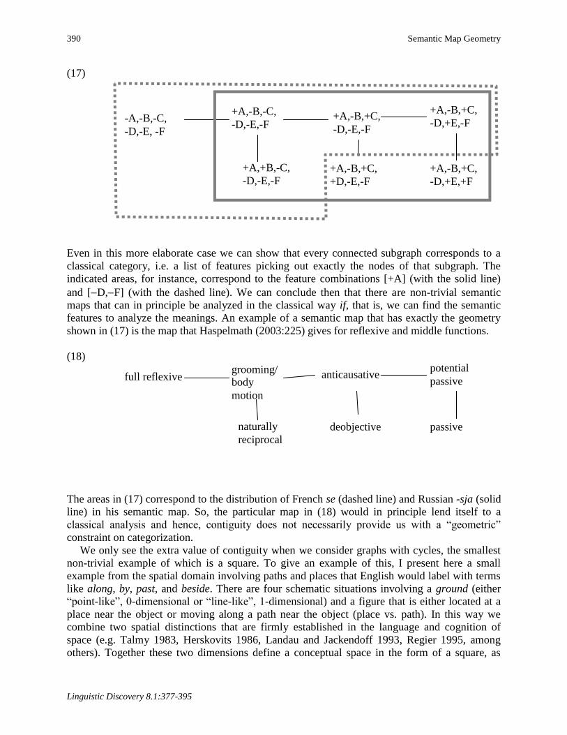
Even in this more elaborate case we can show that every connected subgraph corresponds to a

classical category, i.e. a list of features picking out exactly the nodes of that subgraph. The

indicated areas, for instance, correspond to the feature combinations [+A] (with the solid line)

and [D,F] (with the dashed line). We can conclude then that there are non-trivial semantic

maps that can in principle be analyzed in the classical way if, that is, we can find the semantic

features to analyze the meanings. An example of a semantic map that has exactly the geometry

shown in (17) is the map that Haspelmath (2003:225) gives for reflexive and middle functions.

(18)

full reflexive grooming/

body

motion

naturally

reciprocal

anticausative potential

passive

deobjective passive

The areas in (17) correspond to the distribution of French se (dashed line) and Russian -sja (solid

line) in his semantic map. So, the particular map in (18) would in principle lend itself to a

classical analysis and hence, contiguity does not necessarily provide us with a ―geometric‖

constraint on categorization.

We only see the extra value of contiguity when we consider graphs with cycles, the smallest

non-trivial example of which is a square. To give an example of this, I present here a small

example from the spatial domain involving paths and places that English would label with terms

like along, by, past, and beside. There are four schematic situations involving a ground (either

―point-like‖, 0-dimensional or ―line-like‖, 1-dimensional) and a figure that is either located at a

place near the object or moving along a path near the object (place vs. path). In this way we

combine two spatial distinctions that are firmly established in the language and cognition of

space (e.g. Talmy 1983, Herskovits 1986, Landau and Jackendoff 1993, Regier 1995, among

others). Together these two dimensions define a conceptual space in the form of a square, as

Zwarts 391


shown in (19). In this conceptual space there are four abstract spatial relations (labeled clockwise

from A-D), organized in such a way that relations that share one feature, either on the ground or

the figure dimension, are linked by a line in accordance with the definition given in (16) above.

(19)

What we have here is a simple geometry that is motivated on the basis of conceptual

considerations about figures and grounds although clearly abstracting away from a wide range of

phenomena and questions. It might be far too simple and incorrect in certain respects, but it is a

valid hypothesis about how these meanings are conceptually organized and one that can lead to

clear predictions.

According to the classical theory, there are 9 natural classes here as defined by combinations

of necessary and sufficient features. In the overview in (20) we find the 9 classes as sets of

meanings followed by the features that define them.

(20) Classically defined classes of meanings

{A}: line + path {A,B}: line

{B}: line + place {B,C}: place

{C}: point + place {C,D}: point

{D}: point + path {A,D}: path

{A,B,C,D}: ø (i.e. no features)

Notice that in the classical approach certain classes of meanings cannot be defined, such as

{A,C} and {A,B,C}.

However, if we use the contiguity principle, we get a different, wider collection of classes,

some of which are ―unnatural‖ from the classical point of view (i.e. not definable as a ―checklist‖

of features):



(21) Classes of meanings defined by contiguity

{A}, {B}, {C}, {D}, {A,B}, {B,C}, {C,D}, {A,D}, {A,B,C}, {B,C,D}, {C,D,A},

{A,B,D}, {A,B,C,D}

Because of contiguity, a class of meanings like {A,B,C} is held together by its family

resemblance structure: although meanings A and C do not share any properties, they are taken

together in one category because they both share properties with meaning B, the simplest

instance of a non-classical family resemblance category. {A,C} is an example of a category ruled

out under both perspectives. The question is now whether languages recognize the family

resemblance structure here in using the same adposition, adverb or verb, to label such categories

in (21). It makes sense to ask this question here in this way because we have defined a

conceptual structure for which classical and contiguity-based categorization lead to different

predictions.

English already provides us with an example of the second {B,C,D} situation, as shown by

the following examples (Anna Asbury, p.c.):

(22) A Alex walked along the river. B Alex stood by/beside the river. C Alex stood by/beside the tree. D Alex walked past/by the tree.

Notice that English uses the preposition/adverb by here for the situations B, C, and D. Dutch

provides a different example (based on my own intuitions):

(23) A Alex liep langs de Rivier.

Alex walked along the River

B Alex stond langs/aan/bij de rivier.

Alex stood along/on/by the River

C Alex stond bij de boom.

Alex stood by the Tree

D - Alex liep langs/voorbij de boom/het kampvuur.

Alex walked along/past the tree/the campfire

- Alex liep de boom/het kampvuur voorbij.

Alex walked the tree/the campfire Past

- Alex liep langs

Alex walked along

Notice how the word langs (related to English along) covers the meanings A, B, and D, a

connected subgraph of (19), but not a classical category. We could of course introduce ad hoc

features for the categories {A,B,D} and {B,C,D} to allow for trivial classical definitions, but

(apart from the fact that these might not in any way be motivated by the properties of the four

Zwarts 393


meanings themselves), these features can change the geometry of the conceptual space. More

specifically, for a square-shaped semantic map, like the one in (19), there is no way to model the

effects of contiguity by means of features. This can be seen in the following way. As soon as we

introduce a feature f for the situations A, B, and D and a feature g for the situations B, C, and D,

the distances between the meanings are redefined, and the principle for building the graph

produces more arcs. Two meanings that used to be opposite in the square, namely B and D, are

now going to share two new properties, namely g and f, which motivates a direct link between

them and therefore changes the geometry. Hence, it is not possible to give a feature

decomposition for a square-shaped semantic map that can give us the categories which

contiguity defines without changing the geometry. So, contiguous categories cannot always be

reduced to classical categories. There are many semantic maps that contain squares, like

Haspelmath‘s indefinite pronoun map in (1), where the same reasoning might apply.

What is the difference between the maps in (1) and (19) and the maps in (11) and (18)? I

suspect that it involves an important graph-theoretical difference that lies at the root of this: the

difference between graphs with cycles and graphs without cycles. A cycle is a sequence of nodes

and arcs that allows one to make a complete tour. A graph without cycles is a tree: it branches

without ever connecting to itself again. Why and how exactly cyclicity in meaning similarities

leads to non-classical categorization (by contiguity) is still unclear to me. Note that the smallest

possible cycle (a triangle of meanings, as in (7) above) can be defined in a classical way by

means of three features, so it is not only cyclicity that explains it. This must be left for further

research.

We can conclude that the notion of contiguity (or, more precisely, connectedness), defines

non-classical categories in semantic maps (as long as the underlying conceptual graph has certain

properties). Notice that we can only draw this conclusion because we departed from a purely

matrix-driven approach and considered what the structure of a conceptual space might be, not

derived from the words that are defined over that space but on the basis of the meanings

involved. Moreover, the only way in which we can hope to get a better understanding of the

relation between cyclicity and contiguity is by taking the space-driven approach.

5. Conclusion: Matrix Space

We have seen two opposite approaches to the geometry of conceptual spaces underlying

semantic maps: the matrix-driven approach (which starts from a set of cross-linguistic data) and

the space-driven approach (which starts with a semantic model). In current typological work, the

matrix-driven approach seems most popular for understandable reasons (see section 3).

However, we should be aware of the fact that a purely matrix-driven approach has its limitations,

as I showed in section 4. The matrix-driven approach does not allow us to assess the property of

contiguity itself (the possibility of exceptions and its status as a theory of categorization) because

contiguity is implicit in the inductive procedure. I have not discussed more specific problems

arising with the use of scaling methods that impose a continuous Euclidean structure on all types

of conceptual domains. For these I refer to Zwarts (2008).

There is great value in the matrix-driven approach as a heuristic method. Nevertheless, the

conceptual spaces that are made, either through discrete or continuous methods, should not be

seen as theoretical end points but as a way to help us build semantically-informed models of

conceptual spaces and to reveal the limitations of the purely theory-driven a priori approach.

What we seem to need then, is a closer alliance between the two approaches allowing us to go



back and forth and get a more intensive cross-fertilization of typological and semantic studies.

Only in that way can we better understand what the geometric structure of a particular

conceptual space is like and how it restricts the way languages across the world structure their

grammars and lexicons.

Acknowledgements

This paper was presented at the Workshop on Semantic Maps: Methods and Applications, Paris,

September 29, 2007. I thank the audience there for useful questions and discussion, as well as

Michael Cysouw and one anonymous reviewer for their comments.

References

Berlin, Brent and Paul Kay. 1969. Basic Color Terms: Their Universality and Evolution.

Berkeley: University of California Press.

Brugman, Claudia. 1988. The story of over: Polysemy, semantics and the structure of the

lexicon. New York: Garland Press.

Croft, William. 2001. Radical construction grammar. Oxford: Oxford University Press.

Croft, William and Keith T. Poole. 2008. Inferring universals from grammatical variation:

Multidimensional scaling for typological analysis. Theoretical Linguistics 34/1.1-37

Cysouw, Michael. 2007. Building semantic maps: The case of person marking. New challenges

in typology, ed. by Matti Miestamo and Bernhard Wälchli, 225-248. Berlin: Mouton.

Dalrymple, Mary, M. Kanazawa, Y. Kim, S. Mchombo, and S. Peters. 1998. Reciprocal

expressions and the concept of reciprocity. Linguistics and Philosophy 21/2.159-210.

De Schepper, Kees and Joost Zwarts. 2009. Modal geometry: Remarks on the structure of a

modal map. Cross-linguistic semantics of tense, aspect and modality. ed. by L. Hogeweg, H.

De Hoop and A. Malchukov, 245-269. Amsterdam: Benjamins.

Dewell, Robert. 1994. Over again: Image-schema transformations in semantic analysis.

Cognitive Linguistics 5.351-380.

Gärdenfors, Peter. 2000. Conceptual spaces: The geometry of thought. Cambridge, MA: MIT

Press.

Greenberg, Joseph H. 1966. Universals of kinship terminology. Language universals: With

special reference to feature hierarchies, ed. by Joseph Greenberg, 72-87. The Hague:

Mouton.

Haspelmath, Martin. 1997a. Indefinite pronouns. Oxford: Clarendon.

-----. 1997b. From space to time: Temporal adverbials in the world's languages. München:

Lincom.

-----. 2003. The geometry of grammatical meaning: Semantic maps and cross-linguistic

comparison. The new psychology of language, ed. by Michael Tomasello, vol. 2, 211-243.

New York: Erlbaum.

Herskovits, Annette. 1986. Language and spatial cognition: An interdisciplinary study of the

prepositions in English. Cambridge: Cambridge University Press.

Janda, Laura A. forthcoming. What is the role of semantic maps in cognitive linguistics? To

appear in a festschrift for Barbara Lewandowska-Tomaszczyk, ed. by Piotr Stalmaszczyk and

Wieslaw Oleksy.

Zwarts 395


Lakoff, George. 1987. Women, fire and dangerous things: What categories reveal about the

mind. Chicago: University of Chicago Press.

Landau, Barbara and Ray Jackendoff. 1993. ―What‖ and ―where‖ in spatial language and spatial

cognition. Behavioral and Brain Sciences 16.217-265.

Levinson, Stephen and Sergio Meira. 2003. ‗Natural concepts‘ in the spatial topological domain

– Adpositional meanings in crosslinguistic perspective: An exercise in semantic typology.

Language 79/3.485-516.

Majid, Asifa, Melissa Bowerman, Miriam van Staden and James S. Boster. 2007. The semantics

of ―cutting and breaking‖ events: A cross-linguistic perspective. Cognitive Linguistics

18/2.133-152.

Margolis, Eric and Stephen Laurence. 1999. Concepts: Core readings. Cambridge, MA: MIT

Press.

Regier, Terry. 1995. A model of the human capacity for categorizing spatial relations. Cognitive

Linguistics 6/1.63-88.

Regier, Terry, Paul Kay and Naveen Khetarpal. 2007. Color naming reflects optimal partition of

color space. Proceedings of the National Academy of Sciences 104/4.1436-1441.

Sandra, Dominiek and Sally Rice. 1995. Network analyses of prepositional meaning: Mirroring

whose mind–The linguist‘s or the language user‘s? Cognitive Linguistics 6.89-130.

Talmy, Leonard. 1983. How language structures space. Spatial orientation: Theory, research, and

application, ed. by H. Pick and L. Acredolo, 225-282. New York: Plenum Press.

Tyler, Andrea and Vyvyan Evans. 2001. Reconsidering prepositional polysemy networks: The

case of over. Language 77/4.724-765.

van der Auwera, Johan and Plungian, V.A. 1998. Modality‘s semantic map. Linguistic

Typology, 2/1.79-124.

van der Auwera, Johan, Peter Kehayov and A. Vittrant. 2009. Acquisitive modals. Cross-

linguistic semantics of tense, aspect and modality. ed. by L. Hogeweg, H. De Hoop and A.

Malchukov, 271-302. Amsterdam: Benjamins.

Wälchli, Bernhard. 2007. Constructing semantic maps from parallel text data. Unpublished

manuscript, Universität Konstanz.

Zwarts, Joost. 2008. Commentary on Croft and Poole, ‗Inferring universals from grammatical

variation: multidimensional scaling for typological analysis‘. Theoretical Linguistics 34/1.67-

73.

Author‘s contact information:

Joost Zwarts

Opleiding Taalwetenschap

Departement Moderne Talen

Faculteit Geesteswetenschappen

Universiteit Utrecht

Trans 10

3512 JK Utrecht

The Netherlands

[email protected]

mailto:[email protected]

volume 8 semantic map geometry: two issue 1 approaches

Documents