Volumetric Path TracingSteve Marschner

Cornell UniversityCS 6630 Spring 2012, 8 March

Using Monte Carlo integration is a good, easy way to get correct solutions to the radiative trans-fer equation. It is not fast (at least not as naïvely implemented), especially for inhomogeneous or highly scattering media, but it is easy to get the right answer (plus random noise) for complex cases where there pretty much exists no other way to get an artifact-free solution.

Deriving the path tracing algorithm pretty much boils down to applying the Monte Carlo integra-tion framework to the integral form of the volume rendering equation that we derived in the radia-tive transport lectures. As usual, the key to developing correct algorithms is to carefully write down the integrals involved and construct the Monte Carlo estimators systematically.

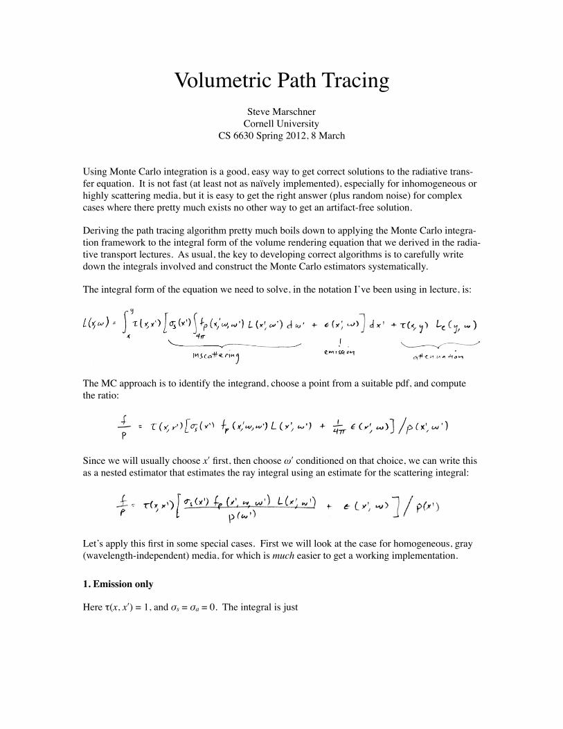
The integral form of the equation we need to solve, in the notation I’ve been using in lecture, is:

The MC approach is to identify the integrand, choose a point from a suitable pdf, and compute the ratio:

Since we will usually choose xʹ′ first, then choose ωʹ′ conditioned on that choice, we can write this as a nested estimator that estimates the ray integral using an estimate for the scattering integral:

Let’s apply this first in some special cases. First we will look at the case for homogeneous, gray (wavelength-independent) media, for which is much easier to get a working implementation.

1. Emission only

Here τ(x, xʹ′) = 1, and σs = σa = 0. The integral is just

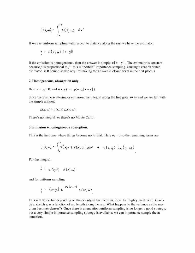
If we use uniform sampling with respect to distance along the ray, we have the estimator:

If the emission is homogeneous, then the answer is simple: ε‖x – y‖. The estimator is constant, because p is proportional to f—this is “perfect” importance sampling, causing a zero-variance estimator. (Of course, it also requires having the answer in closed form in the first place!)

2. Homogeneous, absorption only.

Here ε = σs = 0, and τ(x, y) = exp(– σa‖x – y‖).

Since there is no scattering or emission, the integral along the line goes away and we are left with the simple answer:

L(x, ω) = τ(x, y) Le(y, ω).

There’s no integral, so there’s no Monte Carlo.

3. Emission + homogeneous absorption.

This is the first case where things become nontrivial. Here σs = 0 so the remaining terms are:

.

For the integral,

and for uniform sampling

.

This will work, but depending on the density of the medium, it can be mighty inefficient. (Exer-cise: sketch g as a function of arc length along the ray. What happens to the variance as the me-dium becomes denser?) Once there is attenuation, uniform sampling is no longer a good strategy, but a very simple importance sampling strategy is available: we can importance sample the at-tenuation.

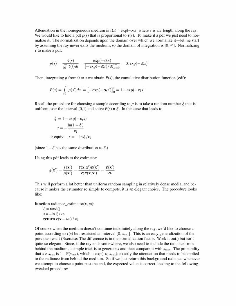
Attenuation in the homogeneous medium is τ(s) = exp(–σt s) where s is arc length along the ray. We would like to find a pdf p(s) that is proportional to τ(s). To make it a pdf we just need to nor-malize it. The normalization depends upon the domain over which we normalize it—let me start by assuming the ray never exits the medium, so the domain of integration is [0, ∞]. Normalizing τ to make a pdf:

p(s) =

τ(s)� ∞0 τ(t)dt

=exp(−σt s)

[−exp(−σt t)/σt ]∞t=0= σt exp(−σt s)

Then, integrating p from 0 to s we obtain P(s), the cumulative distribution function (cdf):

P(s) =

� s

0p(s�)ds� =

�−exp(−σt s�)

�s0 = 1− exp(−σt s)

Recall the procedure for choosing a sample according to p is to take a random number ξ that is uniform over the interval [0,1] and solve P(s) = ξ. In this case that leads to

ξ = 1− exp(−σt s)

s =− ln(1−ξ )σt

or equiv: s =− lnξ/σt

(since 1 – ξ has the same distribution as ξ.)

Using this pdf leads to the estimator:

g(x�) =

f (x�)p(x�)

=τ(x,x�)ε(x�)

σtτ(x,x�)=

ε(x�)σt

This will perform a lot better than uniform random sampling in relatively dense media, and be-cause it makes the estimator so simple to compute, it is an elegant choice. The procedure looks like:

function radiance_estimator(x, ω): ξ = rand() s = –ln ξ / σt return ε(x – sω) / σt

Of course when the medium doesn’t continue indefinitely along the ray, we’d like to choose a point according to τ(s) but restricted an interval [0, smax]. This is an easy generalization of the previous result (Exercise: The difference is in the normalization factor. Work it out.) but isn’t quite so elegant. Since, if the ray ends somewhere, we also need to include the radiance from behind the medium, a simple trick is to generate s and then compare it with smax. The probability that s > smax is 1 – P(smax), which is exp(–σt smax): exactly the attenuation that needs to be applied to the radiance from behind the medium. So if we just return this background radiance whenever we attempt to choose a point past the end, the expected value is correct, leading to the following tweaked procedure:

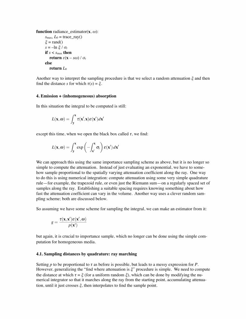
function radiance_estimator(x, ω): smax, L0 = trace_ray() ξ = rand() s = –ln ξ / σt if s < smax then return ε(x – sω) / σt else return L0

Another way to interpret the sampling procedure is that we select a random attenuation ξ and then find the distance s for which τ(s) = ξ.

4. Emission + (inhomogeneous) absorption

In this situation the integral to be computed is still:

L(x,ω) =

� x

yτ(x�,x)ε(x�)dx�

except this time, when we open the black box called τ, we find:

L(x,ω) =

� x

yexp

�−

� x

x�σt

�ε(x�)dx�

We can approach this using the same importance sampling scheme as above, but it is no longer so simple to compute the attenuation. Instead of just evaluating an exponential, we have to some-how sample proportional to the spatially varying attenuation coefficient along the ray. One way to do this is using numerical integration: compute attenuation using some very simple quadrature rule—for example, the trapezoid rule, or even just the Riemann sum—on a regularly spaced set of samples along the ray. Establishing a suitable spacing requires knowing something about how fast the attenuation coefficient can vary in the volume. Another way uses a clever random sam-pling scheme; both are discussed below.

So assuming we have some scheme for sampling the integral, we can make an estimator from it:

g =

τ(x,x�)ε(x�,ω)p(x�)

but again, it is crucial to importance sample, which no longer can be done using the simple com-putation for homogeneous media.

4.1. Sampling distances by quadrature: ray marching

Setting p to be proportional to τ as before is possible, but leads to a messy expression for P. However, generalizing the “find where attenuation is ξ” procedure is simple. We need to compute the distance at which τ = ξ (for a uniform random ξ), which can be done by modifying the nu-merical integrator so that it marches along the ray from the starting point, accumulating attenua-tion, until it just crosses ξ, then interpolates to find the sample point.

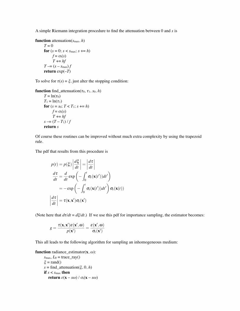
A simple Riemann integration procedure to find the attenuation between 0 and s is

function attenuation(smax, h) T = 0 for (s = 0; s < smax; s += h) f = σt(s) T += hf T –= (s – smax) f return exp(–T)

To solve for τ(s) = ξ, just alter the stopping condition:

function find_attenuation(τ0, τ1, s0, h) T = ln(τ0) T1 = ln(τ1) for (s = s0; T < T1; s += h) f = σt(s) T += hf s –= (T – T1) / f return s

Of course these routines can be improved without much extra complexity by using the trapezoid rule.

The pdf that results from this procedure is

p(t) = p(ξ )����dξdt

���� =����dτdt

����

dτdt

=ddt

exp�−

� t

0σt(x(t �))dt �

�

= −exp�−

� t

0σt(x(t �))dt �

�σt(x(t))

����dτdt

���� = τ(x,x�)σt(x�)

(Note here that dτ/dt = dξ/dt.) If we use this pdf for importance sampling, the estimator becomes:

g =

τ(x,x�)ε(x�,ω)p(x�)

=ε(x�,ω)σt(x�)

This all leads to the following algorithm for sampling an inhomogeneous medium:

function radiance_estimator(x, ω): smax, L0 = trace_ray() ξ = rand() s = find_attenuation(ξ, 0, h) if s < smax then return ε(x – sω) / σt(x – sω)

else return L0

The disappointing thing is that we can’t just plug in a Monte Carlo estimator for the attenuation integral. If it was true that E{exp(X)} = exp(E{X}) then we’d be in good shape—but sadly it is not. This means that the only thing we can do is put in a sufficiently accurate numerical estimate of the integral: we can’t count on statistical averaging to let us use a very noisy estimate.

We also can’t generate an individual sample of s very quickly—we have to integrate along the ray from the eye to the sample point. This means that if we are planning to take many samples along the ray (which, of course, we will need to do), it would be terribly inefficient to handle them in-dependently—in fact, it would be quadratic in the number of samples required.

To generate samples for many values of ξ together, let’s assume that we have the list of random numbers ξ0, …, ξ(n–1) in hand a priori, and that they are sorted so that ξ0 < ξ1 < … < ξ(n–1). To generate the many samples all at once, we can call the integration procedure multiple times, each time picking up from where it left off; you’ll note I added the arguments τ and s0 so that this is easy to do:

function radiance_estimator(x, ω, ξ-list): smax, L0 = trace_ray() S = 0 n = ξ-list.length for (i = 0; i < n; i++) ξ = ξ-list[i] s = find_attenuation(ξ, s, smax, h) if s < smax then S += ε(x – sω) / σt(x – sω) else break return (S + (n – i)L0) / n

(I hope this pseudocode is correct, but as it wasn’t actually transcribed from working code there is some chance of bugs.) Here I am giving the samples that fall past smax (all n–i of them) the value L0 in the average.

Note that it is easy to perform stratified sampling on the ray integral: you just use stratified ran-dom values for the ξi, for instance by splitting the interval up into n pieces and choosing one ran-dom number in each one:

function generate_ξs(n): for (i = 0; i < n; i++) ξs[i] = (i + rand()) / n return ξs

This is easy to do—in fact, easier than generating a sorted list of independent random num-bers—and will perform much better.

Another way to look at this, which makes a lot of sense if evaluating ε is cheap, is that we should just use enough samples that the emission is lost.

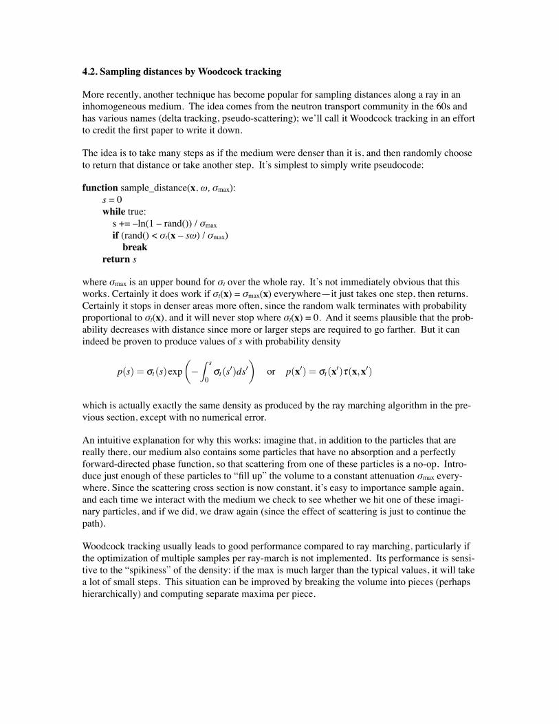
4.2. Sampling distances by Woodcock tracking

More recently, another technique has become popular for sampling distances along a ray in an inhomogeneous medium. The idea comes from the neutron transport community in the 60s and has various names (delta tracking, pseudo-scattering); we’ll call it Woodcock tracking in an effort to credit the first paper to write it down.

The idea is to take many steps as if the medium were denser than it is, and then randomly choose to return that distance or take another step. It’s simplest to simply write pseudocode:

function sample_distance(x, ω, σmax): s = 0 while true: s += –ln(1 – rand()) / σmax if (rand() < σt(x – sω) / σmax) break return s

where σmax is an upper bound for σt over the whole ray. It’s not immediately obvious that this works. Certainly it does work if σt(x) = σmax(x) everywhere—it just takes one step, then returns. Certainly it stops in denser areas more often, since the random walk terminates with probability proportional to σt(x), and it will never stop where σt(x) = 0. And it seems plausible that the prob-ability decreases with distance since more or larger steps are required to go farther. But it can indeed be proven to produce values of s with probability density

p(s) = σt(s)exp

�−

� s

0σt(s�)ds�

�or p(x�) = σt(x�)τ(x,x�)

which is actually exactly the same density as produced by the ray marching algorithm in the pre-vious section, except with no numerical error.

An intuitive explanation for why this works: imagine that, in addition to the particles that are really there, our medium also contains some particles that have no absorption and a perfectly forward-directed phase function, so that scattering from one of these particles is a no-op. Intro-duce just enough of these particles to “fill up” the volume to a constant attenuation σmax every-where. Since the scattering cross section is now constant, it’s easy to importance sample again, and each time we interact with the medium we check to see whether we hit one of these imagi-nary particles, and if we did, we draw again (since the effect of scattering is just to continue the path).

Woodcock tracking usually leads to good performance compared to ray marching, particularly if the optimization of multiple samples per ray-march is not implemented. Its performance is sensi-tive to the “spikiness” of the density: if the max is much larger than the typical values, it will take a lot of small steps. This situation can be improved by breaking the volume into pieces (perhaps hierarchically) and computing separate maxima per piece.

5. Introducing the scattering term

We now know how to handle absorption and emission in the general case. The remaining issue is how to compute scattering. As we’ve observed before, outscattering behaves exactly like absorp-tion, as far as attenuation is concerned. Similarly, inscattering behaves exactly like emission, as far as the integral along the ray is concerned. So we can use the method from the previous sec-tion but modify the emission by adding a Monte Carlo estimator for the scattering integral.

Estimating the scattering integral in a volume is just like estimating the reflection integral at a surface. It is an integral over the sphere, and we will choose directions to sample, thinking of them as points on the sphere.

εs(x�,ω) = σs(x�)

�

4πfp(x�,ω,ω �)L(x�,ω �)dω �

The first thing to try is importance sampling by the phase function. (This means that whenever we propose a particular phase function, we also need to come up with a procedure for sampling it. There is a very simple procedure available for Henyey-Greenstein, the most popular phase func-tion model out there.) Remember the phase function is normalized to be a probability distribution already, so in this case p(ωʹ′) = fp(xʹ′, ω, ωʹ′). Then the estimator is

g(ω �) =f (ω �)p(ω �)

=σs(x�) fp(x�,ω,ω �)L(x�,ω �)

p(ω �)= σs(x�)L(x�,ω �)

So all we need to do is trace a recursive ray to estimate L(xʹ′, ωʹ′) and the process becomes:

1. Choose ξ in [0, 1] and find the point xʹ′ on the ray for which τ(x, xʹ′) = ξ.

2. Choose ωʹ′ according to the phase function.

3. Recursively estimate L(xʹ′, ωʹ′) and compute the estimator (ε(xʹ′, ω) + σs(xʹ′) L(xʹ′, ωʹ′)) / σt(xʹ′).

That is, we simply replace the statement starting S += … by the following:

ωʹ′ = sample_phase_function() Ls = radiance_estimator(x – sω, ωʹ′, new_ξ_list()) S += (ε(x – sω) + σs Ls) / σt(x – sω)

Doing this leads to a path tracing algorithm very similar to a brute-force surface path tracer.

5. Direct lighting for volumes

We just developed the equivalent of BRDF-only sampling in path tracing: it bounces around in the medium and has to coincidentally escape and hit a light source in order to contribute any radi-ance to the image. This works OK as long as lighting is low frequency, but fails badly for small sources. The solution, just as with surface path tracing, is to introduce an importance sampling distribution that expects illumination to come from light sources.

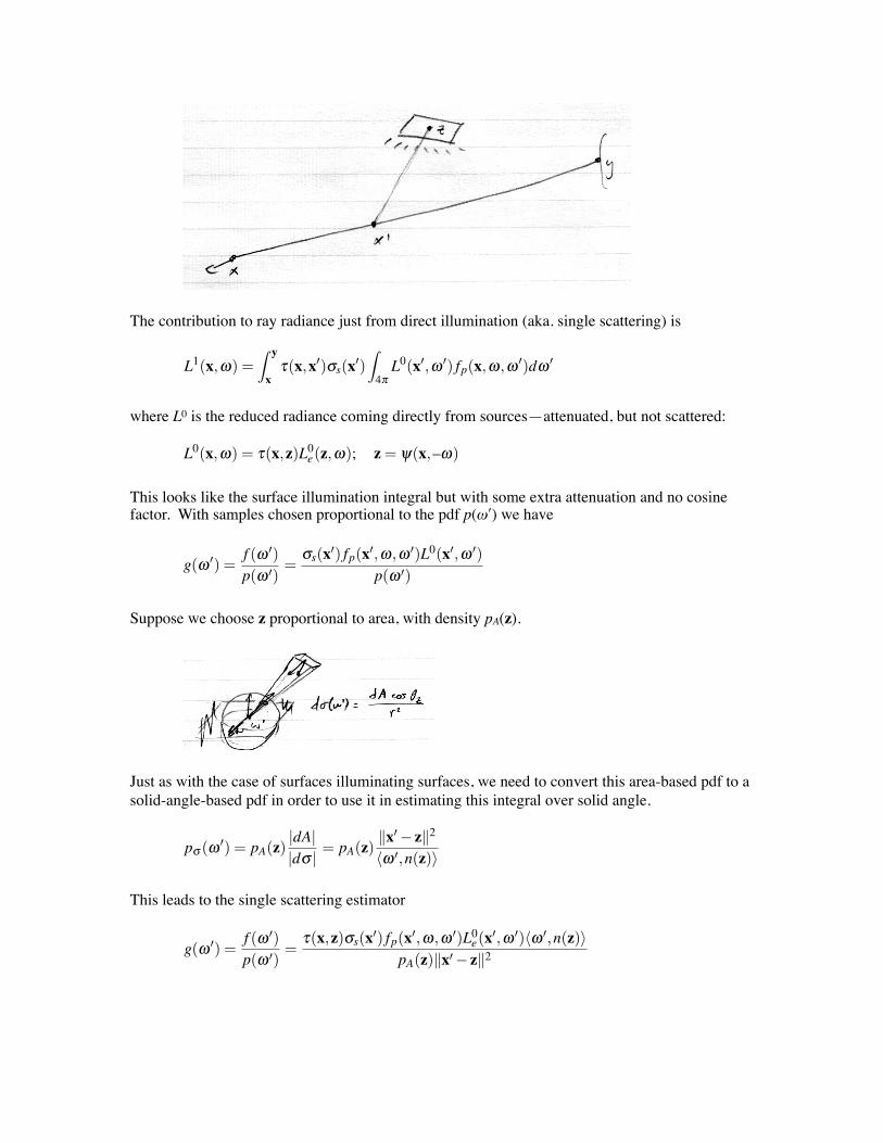
The contribution to ray radiance just from direct illumination (aka. single scattering) is

L1(x,ω) =

� y

xτ(x,x�)σs(x�)

�

4πL0(x�,ω �) fp(x,ω,ω �)dω �

where L0 is the reduced radiance coming directly from sources—attenuated, but not scattered:

L0(x,ω) = τ(x,z)L0e(z,ω); z = ψ(x,–ω)

This looks like the surface illumination integral but with some extra attenuation and no cosine factor. With samples chosen proportional to the pdf p(ωʹ′) we have

g(ω �) =

f (ω �)p(ω �)

=σs(x�) fp(x�,ω,ω �)L0(x�,ω �)

p(ω �)

Suppose we choose z proportional to area, with density pA(z).

Just as with the case of surfaces illuminating surfaces, we need to convert this area-based pdf to a solid-angle-based pdf in order to use it in estimating this integral over solid angle.

pσ (ω �) = pA(z) |dA|

|dσ | = pA(z) �x� − z�2

�ω �,n(z)�

This leads to the single scattering estimator

g(ω �) =

f (ω �)p(ω �)

=τ(x,z)σs(x�) fp(x�,ω,ω �)L0

e(x�,ω �)�ω �,n(z)�pA(z)�x� − z�2

Now we have something that resembles a Kajiya-style path tracer. Adding multiple importance sampling and Russian Roulette requires straightforward generalizations of the methods used for surfaces.